economies of scale and scope in the european banking ... · 1 economies of scale and scope in the...
TRANSCRIPT

1
Economies of scale and scope in the European banking sector 2002-2011
By Mark A. Dijkstra (University of Amsterdam)
Version June 2013 - Preliminary draft
This paper estimates economies of scale and scope for banks within the Eurozone between 2002
and 2011 and attempts to uncover the sources of those economies of scale and scope. Economies of
scale are found to be positive and significant for all years and at all asset levels. When implicit too-
big-to-fail subsidies are accounted for, economies of scale remain positive for the biggest banks
during crisis years, but are negative outside of the crisis. Stronger scale economies are found for
banks that focus on relationship banking compared to those that focus on transaction banking. The
macro environment was found to play an ambiguous role, as the signs differed between simple cost
estimations and more elaborate profit maximizing models. In the profit maximizing models, scale is
found to correlate positively with the quality of ICT infrastructure and market concentration.
Economies of scope are found to be positive for all years and to increase during crisis years. The
results indicate that policy measures that attempt to limit scale and scope in the banking sector
increase costs so that financial stability may be more efficiently guaranteed through other measures.
1. Introduction
Since the start of recent the financial crisis several large financial institutions have received
state aid and concerns have been raised regarding the status these financial institutions as being too-
big-to-fail. Since then, different countries have proposed a variety of measures that limit the scale and
scope of banks through forbidding certain activities,1 explicitly separating financial activities,
2 or
levying additional taxes on banks.3 These measures have in common that they make it more costly for
a bank to undertake additional activities and thus have a detrimental effect on the size and scope of
banks.4 Although these measures may enhance financial stability, they may just as easily not matter
for financial stability,5 while decreasing bank size might have adverse effects on the efficiency of the
financial system. Possible economies of scale and scope6 imply that larger banks might have lower
1 The Volcker rule in the United States is an example of this kind of regulation.
2 For example, the Vickers committee in the United Kingdom advocates ringfencing, which is the legal
separation of retail and investment banking 3 In the Netherlands, policy has been initiated in order to levy a banking tax.
4 President of the Federal Reserve Bank of Dallas Richard W. Fisher (2013) has even proposed to directly limit
the absolute size of banks. 5 See for instance Admati and Hellwig (2011) on the Vickers report, or Admati and Pfleiderer (2012) on the
Volcker rule. 6 Economies of scale imply the cost elasticity to scale is smaller than one, or the profit elasticity to scale is larger
than one. Economies of scope imply lower costs or higher profits as additional activities are undertaken.

2
average costs than smaller banks, which could lead to lower costs for consumers of financial services
of large banks.
Empirical studies on economies of scale in banking have generally found larger economies of
scale over time. Studies that use data from the 1980s and before generally find that economies of scale
are already exhausted at very small bank sizes, of about $100 million in assets.7 Later studies in the
early 1990s have found economies of scale at levels that are higher and higher, such as McAllister and
McManus (1993) who find scale economies up to a size of about $500 million in total assets. Some
studies that focus on the late 1990s and early 2000s find an inverted U-shape for economies of scale
that peaks at higher levels of assets (Carvallo and Kasman, 2005; Tadesse, 2006), thus still suggesting
that there exists a maximum asset size for economies of scale. Finally, there are recent studies that
find economies of scale at the highest asset levels, suggesting that even the largest of banks could
decrease their costs or increase their profits by increasing their scale (Feng and Serlitis, 2010; Hughes
and Mester, 2011; Wheelock and Wilson, 2012). Meanwhile, the evidence of economies of scope in
banks is sparser. A diversification discount is generally found, so that diversified financial
intermediaries are worth less than specialized intermediaries (Laeven and Levine, 2007; Schmid and
Walter, 2009; Berger, Hasan and Zhou, 2010; Cummins et al., 2010). Studies of scale and scope in
banking have typically focussed on data from the United States, although similar evidence is found
from studies that focus on worldwide data.
In this paper economies of scale and scope are estimated for twelve Eurozone countries for
the period 2002 until 2011. Besides estimating the existence of economies of scale and scope, this
paper will make an attempt to disentangle the various sources of economies of scale and scope by
examining the influence of a number of variables that proxy for too-big-to-fail, market power and the
macro-economic environment. This paper adds to the literature on economies of scale and scope in
banking by examining the sources of those economies of scale and scope within a European context.
The Eurozone is considered both because it has a history of relatively large and diversified banks, and
because several policy proposals within Europe aim at limiting scope in banks. This paper is related to
research by Hughes and Mester (2013), who estimate economies of scale in the US in 2003, 2007 and
2010, and Davies and Tracy (2012) who estimate economies of scale for the largest banks in the
world while taking the effect of too-big-to-fail into account. As in those papers, economies of scale
are found to exist, as well as the existence of a too-big-to-fail effect. However, economies of scale are
not completely explained by too-big-to-fail. Besides this, economies of scope are found to be positive
over the entire sample period.
7 Berger and Humphrey (1997) give an overview of 130 of these studies.

3
The rest of the paper is laid out as follows: The second chapter briefly discusses related
literature on economies of scale and scope in banking. The third chapter describes the research
method for the estimation of economies of scale and scope. The fourth chapter describes the data that
is used and from which sources the data was collected. The fifth chapter presents the results. The sixth
chapter discusses the results and describes where the results may be placed within the literature.
Finally, chapter seven concludes.
2. Literature
Boot (2003) and Walter (2003) discuss possible sources of economies of scale and scope in
banking, which can be broadly divided in four groups: i. Economies of scale and scope that are related
to information and communication technology (ICT), ii. Economies of scale and scope that arise
through reputation and branding, iii. Innovation related economies of scale and scope, and iv.
Diversification of risk. Economies of scale and scope related to ICT generally have to do with
spreading fixed overhead costs of ICT over a larger amount of operations, for instance through the
processing of transactions or offering different products through the same distribution channel.
Reputational and banding economies arise because a wider range of products can profit from the same
(generally fixed cost) reputation and brand. And a larger scale and scope will also help in making a
profit from investment in R&D, which generally is a fixed cost.
Diversification of risk as a source of economies of scale and scope is more controversial.
Traditional finance theory states that diversification will not bring any advantages to the firm as long
as investors can costlessly diversify their own portfolios. In that case, investors will not pay a
premium for diversified firms. This argument might hold less weight for a financial intermediary, for
which trust is important. For instance, diversification might alleviate the possibility of a bank run
because of investor trust in a bank’s ability to withstand idiosyncratic shocks. Diversification might
also seem beneficial ex ante, but harmful ex post. Milbourn, Boot and Thakor (1999) show that
expansions into new markets can be thought of as real options. Entering a new market might open up
the possibility for first-mover advantages and as such entering a market has a positive option value for
a firm. If multiple players decide to seek these options, the value of the option might not be taken into
account when measuring economies of scope, thus resulting in negative ex post economies of scope,
even though they are positive ex ante.
Aside from these possible real economies of scale and scope, an artificial scale advantage can
come about for large financial institutions when they become too big to fail (TBTF). When the
bankruptcy of a very large (or very connected) financial institution has a negative impact on the

4
financial system as a whole, the government might have no choice but to save the financial institution
in case of default. This creates a de-facto insurance against bankruptcy for these large financial
institutions, thus allowing them to borrow at lower cost. Furthermore, when scale or scope is achieved
through mergers and acquisitions, market concentration might increase, leading to the possibility of
monopolistic rents. Economies of scale and scope arising from market power and implicit too-big-to-
fail subsidies might benefit individual institutions, but harm society as a whole.
Furthermore, not all banking activities might be susceptible to economies of scale. Walter
(2003) asserts that transaction banking activities are generally scalable, and Boot and Ratnovski (2012)
state that trading activities (a prime example of a transaction banking activity) are especially scalable.
This is contrasted to relationship banking, which focuses on building a relationship with a customer.
Relationship building generally features very little fixed costs as each new client requires new effort
and as such is not very scalable. In fact, smaller banks might be advantaged in relationship activities.
Berger et al. (2005) show that if a bank is a branch to a larger conglomerate, it will not have all of the
capital decisions and as such will be less incentivized to create soft information about clients, because
it might not be able to profit from client information if that branch is not allocated capital
appropriately. In contrast, when a bank stands on its own, it will be more incentivized to create soft
information. The crucial assumption is that soft information can’t be credibly passed on into the
command chain. When it is possible to harden information and credibly pass it on, the opposite can
happen: if a bank possesses quality hard information, it might be able to attract more capital as part of
a branch when compared to the situation in which it has to attract its capital on the market. As
relationship banking is concerned with creating soft information and transaction banking relies on
hard information, economies of scale are expected in transaction banking activities, but not in
relationship banking activities.
The macro environment might also play a role in the possibility of creating economies of
scale. Bossone and Lee (2004) show that banks that operate in larger financial markets generally
enjoy more economies of scale than those that operate in smaller markets. The authors show that
macro variables such as the size of the financial sector and stock market capitalization play a positive
role in the determination of economies of scale for banks.
Anderson and Joevier (2012) show that economies of scale might not only lead to higher
rewards to shareholders in the form of higher profits, but may also lead to higher rewards to bank
management in the form of additional wages. Therefore, wages may be considered either as an input
or output in the production process. Anderson and Joevier (2012)’s estimations are based on OLS-
regressions that assume a linear relation between returns to managers and shareholders and several
inputs, while not estimating the cost function of a bank. An approach that estimates bank costs such as

5
a translog cost or profit function while treating the wage bill as an output rather than an input might
shed more light on possible economies of scale that accrue to managers.
Real economies of scale and scope might be difficult to empirically disentangle from artificial
economies of scale and scope. Proxies might be taken in order to account for these different possible
sources of economies of scale and scope. Table 1 presents the issues in estimating economies of scale
and scope in banking as well as the possible proxies that can be taken in order to control for these
issues.
Table 1: Issues in estimating economies of scale and scope in banking.
Key issue Hypothesis Proxy
Risk frontier Bigger banks might have access
to a higher risk-return frontier
Equity capital, nonperforming
loans, loan loss reserves
ICT Information technology
enhances economies of scale
Broadband connections per
capita
Brand/ Reputation Brand and reputation scale as a
fixed cost
Innovation Innovation benefits can be
spread out over a larger scale
R&D expenditure
Too big to fail TBTF subsidies cause
economies of scale
Dummy for assets>$100 bln
Moody’s rating difference
Market power Monopoly power causes
economies of scale
CR3/4/5, HHI
Relationship banking Relationship banking is not
scalable
Interest income
Transaction banking Transaction banking is scalable Trading income, commission
income
Systemic scale economies Scale economies are bigger in
bigger financial markets
GDP, Size of the financial
sector
Physical distance Higher physical distance means
less scalability
Population density
Scale economies to managers Scale economies might benefit
managers
Wages as an output
Scope diversification Diversification leads to
economies of scope
Specialization index
Scope coordination problems Engaging in multiple activities
might harm firm value
Specialization index
Scope as a strategic option Expansions in new markets
might be used as options
Firm growth Firms grow faster when
financed by universal banks
TFP
First of all, Hughes and Mester (2013) state that not including risk in the estimation of
economies of scale might lead to incorrect estimates. Larger banks may be perceived as less risky and
as such have access to a higher risk-return frontier. In that case, a larger bank might be inclined to
hold a different asset portfolio (for instance by holding less liquid assets than a smaller bank).

6
Depending on the specification, this may lead to a lower estimate of economies of scale for large
banks when risk is not explicitly accounted for. As a proxy for risk, equity capital can be included as
well as nonperforming assets and loan loss reserves. The effect of risk may also require a different
model specification altogether.
Marinč (2013) argues that the increase of scale economies might be mostly influenced by
improvements in ICT technology, which improve information processing within a bank. Some
activities might be better scalable than others, with hard information products benefitting more in
terms of scalability than soft information products. Boot (2003) mentions that information technology
presents the greatest possible source of scale economies by better use of databases over a wider range
of services and customers. It is not entirely clear how the use of ICT in financial intermediaries should
be proxied, since high ICT expenditure might mean either a large commitment to ICT, or an
inefficient ICT department. The ICT infrastructure that a bank operates in may provide a good proxy
for the quality of ICT that is available to bank, as a better infrastructure possibly allows for lower
costs of employing ICT. Proxies for the ICT infrastructure are the number of broadband connections
per capita, or the percentage of internet users.
The effect of too-big-to-fail has been traditionally proxied by using dummies that are equal to
one when a bank crosses a certain asset or market capitalisation threshold. For instance, Brewer and
Jagtiani (2011) assume that banks with either $100 billion in assets or $20 billion in equity capital are
too big to fail. Recent work by Ueda and Weder di Maurer (2012), Davies and Tracy (2012) and
Bijlsma and Mocking (2013) focuses on a different proxy that is outlined by Haldane (2010). These
authors take differences in Moody’s ratings for banks as standalone entities and the ratings for those
same banks when possible government support is taken into account. By taking the difference
between these ratings, a proxy for the size of the implicit funding subsidy can be found.
Market power in banking is generally proxied by taking the Herfindahl-Hirschman index
(HHI), which takes the sum of quadratic asset shares of banks within a country or region, or
concentration ratios (CR3/4/5), which measure the share of total assets within a country held by the
biggest four, five or six banks.
The share of trading income or commission income in total income might prove a good proxy
for the amount of transaction banking activities in a bank and should generally be associated with
larger economies of scale. Meanwhile, relationship activities generally take the form of interest
contracts that pay off over a longer term and as such the share of interest income in total income
might be a good proxy for the amount of relationship banking activities, and should generally be
negatively correlated with economies of scale.

7
Degryse and Ongena (2005) show that physical distance is an important determinant with
respect to a consumers choice for a bank. Costs of monitoring could be determined by physical
distance. Since setting up a branch means incurring a fixed cost, population density around that
branch might imply economies of scale. Berger et al. (2005) however note that generally big banks
are better at managing relationships at a distance, thus justifying larger scales in countries that have
large physical distances from bank to client. Average distance to a client within a country might be
proxied by population density.
Neuhann and Saidi (2012) mention the possibility of economies of scope in financing companies.
By issuing both debt and equity, a bank might be able to lessen the impact of moral hazard from
multiple sources. A debt contract induces truth-telling, while equity underwriting might alleviate debt
overhang problems. They find that universal banks tend to invest in riskier firms, that have higher
TFP growth than firms that were invested in by specialized banks. TFP growth within a country might
be a result of broader banking.
Empirical evidence on economies of scale and scope
Empirical studies on scale in banking from the 1980s and 1990s generally find that the
relationship between economies of scale and asset size displays an inverted U shaped pattern. In those
studies economies of scale are exhausted at a relatively low level of around $100 million to $500
million in total assets (Berger and Humphrey, 1997; McAllister and McManus, 1993). Over time, the
estimate for the asset size at which economies of scale are exhausted has gone up to around $10
billion to $25 billion, but generally still tended to find an inverted U shaped relationship between
scale and asset size (Berger and Mester, 1997; Hughes, Mester and Moon, 2001).
The most recent studies using data past 2000 tend to find economies of scale at higher levels, even
for the largest of banks (Feng and Serlitis, 2010; Hughes and Mester, 2011; Wheelock and Wilson,
2012). The fact that economies of scale are found at higher and higher levels in the literature, may be
due to econometric improvements, or if the financial environment has changed, due to technological
progress through ICT improvements and financial deregulation such as the Gramm-Leach-Bliley Act
(Mester, 2010). Marinč (2013) argues that the increase of scale economies might be mostly influenced
by improvements in ICT technology, which greatly improves information processing within a bank.
Davies and Tracy (2012) however find that when proxies are introduced for implicit governmental
subsidies, economies of scale disappear and as such show that economies of scale are mostly driven
by too-big-to-fail effects.
Although the literature has generally been favourable towards the existence of economies of scale
in banking, the same cannot be said about economies of scope. Generally diseconomies of scope are

8
found: Laeven and Levine (2007) and Schmid and Walter (2009) find that conglomerates that engage
in multiple activities are valued less by financial markets than specialized institutions. Berger, Hasan
and Zhou (2010) and Cummins et al. (2010) find diseconomies of scale through efficiency measures.
Why economies of scale materialize but economies of scope do not, is less clear. Diversification
benefits might be insufficient to make up for additional costs, agency costs could be higher when
activities are stretched over multiple markets, or there may be specialization benefits that are foregone
when multiple activities are engaged in. Also, improvements in the ICT environment may make
scaling up more profitable, rather than saving costs over multiple activities.8
The next chapter will describe the three methods that are used in this paper to estimate economies
of scale and scope within Europe.
3. Method
Economies of scale are estimated in this paper by using three methods: i. a baseline cost
economies of scale estimation; ii. a cost economies of scale estimation that takes the costs of equity
into account, and iii. an adaptation of a managerial preference model, based on Hughes and Mester
(2013). As a baseline, economies of scale are estimated using a basic translog cost function.
( ) ∑
⁄ ∑ ∑
( )
Where:
Total costs
Vector of input quantities ( )
Vector of output quantities ( )
Vector of other inputs
For the baseline estimation of economies of scale, only loan loss reserves are included in in
order to control for asset quality and risk. Equity capital is not considered as an input. To control for
8 Also, Boot (2003) argues that mergers directed at economies of scope might come about strategically to
combat business uncertainty. When there are first-mover advantages for entering new markets, firms may
estimate positive economies of scope ex ante, that might lead to overinvestment, and as such turn out negative
ex post.

9
macro factors that possibly affect economies of scale, proxies are included in to take into account
the size of the financial sector, the amount of competition, ICT infrastructure, population density and
capitalization of the stock market. On the bank level, the composition of income over interest and
commissions income is considered. These variables proxy for relationship and transaction banking
activities. Commission income is more associated with transaction banking, while interest income
might be more associated with relationship banking. From this function, economies of scale are
estimated by:
∑
This is the inverse of the elasticity of costs to output so that this measure is bigger than 1 in the case
of increasing returns to scale and smaller than 1 in case of decreasing returns to scale. This measure
serves as a baseline for comparing the other measures of scale that will be discussed below.
If equity is included in the estimation of scale economies, the cost function to estimate stays
similar:
( ) ∑
⁄ ∑ ∑
( )
In this specification, equity (k) is included in . If economies of scale are estimated in the
same manner as the baseline cost estimation, a constant price of equity is assumed. However, the price
of equity becomes lower as the amount of equity increases through the Modigliani and Miller (1958)
theorem. Similarly, when large institutions are perceived as less risky because of diversification
benefits, their equity might have a lower price. Ignoring the price of equity will underestimate
economies of scale for larger banks: large institutions with smaller amounts of equity will have higher
interest costs, because they are financed more with debt, so that costs are overestimated. By correcting
for the price of equity, economies of scale are estimated by:
∑
Besides these scale estimations that are based on translog cost functions, a third estimation of
economies of scale is made, based on a methodology proposed by Hughes and Mester (2013).9 These
9 The authors have used this method before in Hughes et al. (1996; 2000), and Hughes, Mester and Moon (2001).

10
authors use a managerial preference model, modelled by an adaptation of the Almost Ideal Demand
System, which was first introduced for consumer goods by Deaton and Muellbauer (1980).10
Instead
of preferences over different consumer goods, Hughes and Mester (2013) use the basis of the almost
ideal demand system in order to model the preferences of managers over inputs and outputs in the
production process. By observing output quantities and input prices, the cost elasticities to outputs can
be found. Inverted cost elasticities can then be used to see whether a bank is operating under
increasing or decreasing economies of scale. The managerial preference model formulates a standard
utility maximizing problem that is faced by the manager:
( )
( )
The variables are:
Profit
Vector of input quantities ( )
Vector of output quantities ( )
Amount of nonperforming loans
Vector of output prices ( )
Risk-free interest rate
Amount of equity capital
Vector of input prices ( )
Vector of other inputs ( )
Average interest rate on assets
Combined corporate tax rate
This optimization problem means that the manager maximizes his utility, which may mean
either profit maximization or cost minimization, or a combination of both. In a sense, profit
maximization is a better measure than cost minimization, since the objective of the firm as a whole is
10
The purpose of the almost ideal demand system is to empirically estimate preferences of consumers over
goods, using the data on observed consumption and prices. By estimating the demand function for each good
together with the budget function, the elasticity of demand for a certain good can be calculated from the
estimation results

11
profit maximization, and the output level at which profit is maximized may not coincide with the
output level at which costs are minimized. Furthermore, profit maximization may be a more
appropriate goal at the consolidated level of the holding company, while cost minimization might be
more appropriate at the branch level of banking. The contributions to profit by managers at the branch
level might not be easily acquired, so that branch managers are instead incentivized to minimize costs
(Berger and Mester, 1997). Profit maximization is taken as the relevant goal because data is collected
at the highest consolidated level. From the utility maximization problem, the indirect utility function
can be taken. Taking first order conditions from the indirect utility function results in a system of
equations that can be estimated:
[ ( ) ] (Profit)
[ ( ) ] (Input)
( )
( )
(Equity)
The (Profit) equation states that the manager maximizes profits, while the five (Input)
equations state that inputs are chosen optimally, and the (Equity) equation ensures that the capital
structure is also optimally chosen in order to maximize profit. By explicitly modeling the (Equity)
equation, the manager can optimally choose the leverage of the firm, taking into account the
possibility of the risk-return frontier changing with bank size. Appendix A lists the variables more in-
depth. Together, these equations can be empirically estimated by nonlinear regression. The system of
equations to be estimated empirically is:
∑ ∑ ∑ [ ( ) ] (Profit)
∑ ∑ ∑ [ ( ) ] (Inputs)
∑ ∑ ∑ [ ( ) ] (Equity)
The equations are fully written out in Appendix B. This estimation is referred to as the
managerial preference function in the rest of the paper.
∑ [
]
∑ [
]

12
These equations are subtly different from a translog cost functions that are described above.
The translog cost functions specify the cost function in a way that imposes as little structure as
possible on the data, since the exact cost function is generally not known. The managerial preference
model imposes restrictions on the optimization behavior of the manager. The translog cost functions
thus have more freedom in estimating the cost function. However, this may imply that the cost
function that is estimated is not actually the cost function that is available to the manager. In order to
estimate the decision that is available to the manager, more structure is needed. Besides this, the
traditional translog cost function assumes a constant risk return frontier. This may not be the case, as
larger financial institutions might be more diversified and thus could choose a higher risk return
frontier. In that case, a traditional translog cost function might overestimate the costs of risk
management compared to the benefits of taking additional risk at higher asset levels, and as such
underestimate economies of scale at high levels of assets. Finally, the managerial preference function
assumes profits are maximized instead of assuming costs are minimized like the translog cost
functions do.11
Economies of scope
Besides economies of scale, economies of scope are estimated as well. Scope economies
measure if it is less costly for firms to produce a multitude of outputs rather than focusing on a single
output. Economies of scope can be estimated by comparing costs of the multiproduct firm with costs
of the firm were it specialized in several smaller firms each specialized in a single output:
∑ ( ) ( )
( )
Where ( ) is the relevant cost function for each of the three specifications. If this
measure is greater than zero, costs would be larger if the firm was specialized in multiple specialized
firms, so that economies of scope exist, while a measure below zero implies diseconomies of scope.
Mester (2008) argues that this measure of economies of scope is not correct. It evaluates economies of
scope at a zero output level, so that it can’t be used to evaluate translog cost functions because
logarithms of zero do not exist. Besides this, it forces costs to be evaluated at zero output levels even
when all firms are producing positive levels of each output, so that results are extrapolated outside of
11
Inverse cost elasticities to scale are later estimated rather than profit elasticities. This makes it easier to
compare the results to traditional translog cost functions, and may be more relevant since cost economies of
scale might signify possible improvements to consumers, while profit economies might mostly signal possible
improvements to shareholders.

13
the sample. Mester (2008) therefore proposes a measure for economies of scope per bank to be
calculated by:12
∑ ( ( )
)
( )
( )
So that the costs to produce the output by the firm are compared to what it would cost to operate
five firms that specialize in one output and produce the minimal amount of the other outputs.13
If a
bank is better off splitting up into multiple specialized banks, the measure will be negative, as costs
for the specialized banks will be lower than costs for the bank offering all services. This measure of
scope economies that will be evaluated here, for all of the three specifications of the cost function (the
two translog functions and the managers most preferred cost function).14
All measures of economies of scale and scope are estimated using data from banks in the euro
area between 2002 and 2011, for which the data is described in the next chapter.
4. Data
Data on the level of individual banks is obtained from Bureau van Dijk’s Bankscope. Data is
collected for countries in the euro area between 2002 and 2011.15
The year 2002 was chosen as a
starting point as it was the first year in which the euro was introduced as a physical currency, and
2011 is the last year for which data is available. The group of countries was chosen as these countries
have been in the Eurozone over the entire period and as such use a common currency and are under
similar rule of law. A minimum threshold level of assets is not considered in this paper, as policy
proposals that aim to split up banks or forbid certain activities affect banks at all asset levels. In total,
Bankscope features 42,493 observations for these countries over this period. Of these, 374 did not use
the euro as their base currency, and as such were taken out, leaving 42,119 observations. For
estimation, logarithms of input and output quantities need to be taken, so that banks with non-positive
values for inputs and outputs needed to be taken out. This left 20,144 bank level observations. Finally,
Bankscope features some double observations, in which bank subsidiaries were measured both at the
holding level and at the subsidiary level. These double observations were taken out, leaving 18,639
12
This measure was first proposed by Mester (1991). 13
Note that some observations for banks that operate near the minimum output will fall out, as their specialized
production will become a negative number, of which the logarithm doesn’t exist. This is the case for around five
percent of the observations. 14
Economies of scope might also be evaluated by looking at the second derivatives of the cost function. In that
case, a positive value means that adding to one input increases the marginal costs of other products, which
implies diseconomies of scope. Similarly, a negative value implies economies of scope. 15
Austria, Belgium, Finland, France, Germany, Greece, Ireland, Italy, Luxembourg, Netherlands, Portugal and
Spain.

14
observations. Finally, the data was checked for outliers, which resulted in the removal of one
observation where loan loss reserves were larger than total liabilities.
Bankscope features yearly data that is taken from the annual reports of banks. This implies that
data is available on quantities, and not on prices. Previous authors using the Bankscope database have
used the input quantity over assets as a proxy for the input price.16
Input quantities might feature
larger outliers in the data compared to input prices, because some small banks have very high asset
specializations, which could affect their input mix enormously, and as such give scale measures that
may be higher than what would be expected when using input prices.
To estimate the cost functions, five outputs are selected: y1 which are liquid assets; y2 comprising
of the total amount of securities; y3 loans; y4 other earning assets; and y5 off balance sheet items. The
six intputs are: x1 expenses on personnel; x2 fixed assets; x3 demand deposits; x4 savings deposits; x5
other earning assets; and k equity capital. Revenue is the sum of all interest and non-interest income,
costs is total interest and non-interest expense, and profits are defined as revenue minus costs. Ex ante
asset quality is proxied by p the average interest rate on assets and n the amount of loan loss reserves,
where riskier assets are assumed to earn a higher interest or require higher loss reserves.
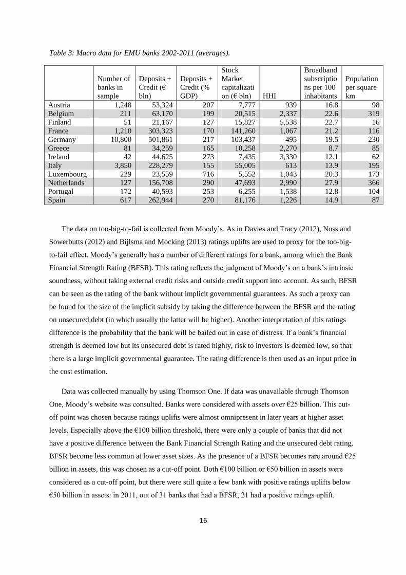
Table 2 presents the data. On average, banks in the sample have an asset size of €14 billion, with
the smallest bank in the sample holding €15 million in assets ranging to the largest bank in the sample
(Deutsche Bank in 2008) which holds €2.2 trillion in assets.
16
This is often done in the literature that studies banking outside of the US. Examples include Lensink, Meesters
and Naaborg (2008); Berger, Klapper and Turk-Ariss (2009); Barth et al. (2010); and Feng and Serletis (2010).

15
Table 2: Data for EMU banks 2002-2011 (n=18,638).
Variable Mean Median Std Dev Minimum Maximum
Total Assets in € mlns 14,341 879 83,382 15 2,202,423
Total Revenue in € mlns 693
50
42
3,683
1
98,712
Financial Performance
Equity Capital/Assets 0.070 0.061 0.036 0.000 0.575
Loan Loss Reserves/Assets 0.005 0.004 0.005 0.000 0.263
Profit/Revenue 0.184
0.182
0.096
-3.156
0.785
Profit/Assets 0.011
0.010
0.011
-0.376
1.014
Asset Allocation
Liquid Assets: y1/Assets 0.168 0.136 0.127 0.002 0.977
Securities: y2/Assets 0.202 0.188 0.124 0.000 0.935
Loans: y3/Assets 0.604 0.623 0.160 0.000 0.989
Other Earning Assets: y4/Assets 0.346 0.329 0.159 0.003 0.989
Off Balance Sheet Items: y5/Assets 0.119 0.061 0.525 0.000 33.969
Input Utilization
Personnel Expenses: x1/Assets 0.013 0.013 0.006 0.000 0.177
Physical Capital: x2/Assets 0.014 0.013 0.010 0.000 0.547
Demand Deposits: x3/Assets 0.252 0.231 0.143 0.000 0.907
Savings Deposits: x4/Assets 0.355 0.413 0.210 0.000 0.943
Other Borrowed Funds: x5/Assets 0.114 0.058 0.138 0.000 0.930
Prices
Tax Rate 0.285 0.264 0.034 0.125 0.344
1/(1-Tax Rate) 1.401 1.358 0.068 1.143 1.525
Macro level data is taken from Bankscope, World Bank, International Telecommunications Union
(ITU), and Mayer and Zignago (2011). The country level data is presented in table 3 below. The
dataset is dominated by German banks. This is because the dataset features a lot of small cooperative
banks,17
for which Bankscope does not provide consolidated data. Detailed information on the
datasources is given in Appendix C.
17
These include the Sparkassen.
16
Table 3: Macro data for EMU banks 2002-2011 (averages).
Number of
banks in
sample
Deposits +
Credit (€
bln)
Deposits +
Credit (%
GDP)
Stock
Market
capitalizati
on (€ bln) HHI
Broadband
subscriptio
ns per 100
inhabitants
Population
per square
km
Austria 1,248 53,324 207 7,777 939 16.8 98
Belgium 211 63,170 199 20,515 2,337 22.6 319
Finland 51 21,167 127 15,827 5,538 22.7 16
France 1,210 303,323 170 141,260 1,067 21.2 116
Germany 10,800 501,861 217 103,437 495 19.5 230
Greece 81 34,259 165 10,258 2,270 8.7 85
Ireland 42 44,625 273 7,435 3,330 12.1 62
Italy 3,850 228,279 155 55,005 613 13.9 195
Luxembourg 229 23,559 716 5,552 1,043 20.3 173
Netherlands 127 156,708 290 47,693 2,990 27.9 366
Portugal 172 40,593 253 6,255 1,538 12.8 104
Spain 617 262,944 270 81,176 1,226 14.9 87
The data on too-big-to-fail is collected from Moody’s. As in Davies and Tracy (2012), Noss and
Sowerbutts (2012) and Bijlsma and Mocking (2013) ratings uplifts are used to proxy for the too-big-
to-fail effect. Moody’s generally has a number of different ratings for a bank, among which the Bank
Financial Strength Rating (BFSR). This rating reflects the judgment of Moody’s on a bank’s intrinsic
soundness, without taking external credit risks and outside credit support into account. As such, BFSR
can be seen as the rating of the bank without implicit governmental guarantees. As such a proxy can
be found for the size of the implicit subsidy by taking the difference between the BFSR and the rating
on unsecured debt (in which usually the latter will be higher). Another interpretation of this ratings
difference is the probability that the bank will be bailed out in case of distress. If a bank’s financial
strength is deemed low but its unsecured debt is rated highly, risk to investors is deemed low, so that
there is a large implicit governmental guarantee. The rating difference is then used as an input price in
the cost estimation.
Data was collected manually by using Thomson One. If data was unavailable through Thomson
One, Moody’s website was consulted. Banks were considered with assets over €25 billion. This cut-
off point was chosen because ratings uplifts were almost omnipresent in later years at higher asset
levels. Especially above the €100 billion threshold, there were only a couple of banks that did not
have a positive difference between the Bank Financial Strength Rating and the unsecured debt rating.
BFSR become less common at lower asset sizes. As the presence of a BFSR becomes rare around €25
billion in assets, this was chosen as a cut-off point. Both €100 billion or €50 billion in assets were
considered as a cut-off point, but there were still quite a few bank with positive ratings uplifts below
€50 billion in assets: in 2011, out of 31 banks that had a BFSR, 21 had a positive ratings uplift.

17
Ratings were given numerical values, starting at 1 for the rating C (lowest), up until 21 for the
Aaa rating. The ratings uplift was calculated by taking the difference between the rating on (senior)
unsecured debt and the BFSR. If data on unsecured debt was unavailable, the rating on long term
deposits was taken instead. Only positive implicit subsidies were considered, so that a negative
difference was given the value zero. If a BFSR could not be found, no ratings uplift was assigned.
Table 4 gives and overview of the ratings uplift data. Most striking is the change in ratings uplifts
around the crisis. Not only are there more banks that are deemed too big to fail18
(that have a positive
ratings uplift), but the average size of the ratings uplift also increases slightly.
Table 4: Ratings uplift data (difference between Moody’s unsecured debt rating and BFSR).
Number of banks with
a ratings uplift Average ratings uplift
Average assets of
TBTF banks (€ bln)
2002 23 3.3 121
2003 33 3.2 141
2004 30 2.7 136
2005 30 2.4 141
2006 34 2.9 155
2007 82 2.5 208
2008 107 3.1 222
2009 102 4.0 197
2010 97 3.8 194
2011 76 3.1 235
5. Results
This chapter presents the estimates for economies of scale and scope for three model
specifications and with inclusion of different control variables.
Economies of scale
Economies of scale are estimated separately for each year. This was done because the cost
frontier might differ from year to year. Also, since a new sample of banks is considered for each
year survivor bias is limited as firms that go bankrupt are not excluded out of the sample. Table 5
shows scale estimates per year. These estimates are graphically represented in figure 1. For the
complete sample, the translog cost functions show diminishing economies of scale over time. In
these functions economies of scale start off positive, but turn into diseconomies of scale around
18
Contributing to this difference is the fact that less data was available for earlier years. However, this is still
mainly driven by the actual data. For reference: about 20% of the banks for which a BFSR rating could be found
had zero uplift in 2011, compared to about 65% in 2002.

18
the time when the financial crisis starts. This result is not shared by the managerial preferences
function, which estimates significant economies of scale over the entire period that go up over
time. This might mean that risk management has become more important since the crisis, so that
the possibilities of risk diversification because of a larger size play a more important role.
Table 5: Economies of scale (inverse elasticities of costs to scale) for 12 EMU countries in the
period 2002-2011, all banks.
All banks 2002 2003 2004 2005 2006 2007 2008 2009 2010 2011
Baseline estimation
1.022
(.001) 1.018
(.001) 1.024
(.001) 1.009
(.001) 1.007
(.001) .998
(.001) .998
(.001) .990
(.001) .991
(.001) .985
(.001)
Equity included
estimation 1.011
(.001) 1.017
(.001) 1.016
(.001) 1.008
(.001) 1.010
(.001) 1.003
(.001) 1.005
(.001) 1.012
(.001)
1.000
(.001) .983
(.001)
Managerial preferences
estimation 1.160
(.007) 1.168
(.006) 1.174
(.006) 1.204
(.006) 1.209
(.006) 1.204
(.011) 1.197
(.010) 1.239
(.019) 1.219
(.013) 1.271
(.009)
N 2205 2050 1928 1951 1844 1892 1934 1880 1796 1158
Standard errors are reported between brackets. Bold numbers indicate that the measure is significantly different
from 1 at the 1 percent level; **
at the 5 percent level; * at the 10 percent level.
Figure 1: Economies of scale per year.
Table 6 shows the measures of scale economies per country. Finland has the highest economies of
scale, while Ireland has the lowest on average. Each country has a banking sector that on average
experiences economies of scale.
0.950
1.000
1.050
1.100
1.150
1.200
1.250
1.300
2002 2003 2004 2005 2006 2007 2008 2009 2010 2011
Baseline estimation
Equity included estimation
Managerial preferences estimation

19
Table 6: Economies of scale per country (inverse elasticities of costs to scale) for 12 EMU
countries in the period 2002-2011.
Baseline
estimation
Equity included
estimation
Managerial
preferences
estimation
Austria 0.979 0.973 1.215
Belgium 0.995 1.022 1.210
Finland 0.977 0.946 1.534
France 0.995 1.002 1.373
Germany 1.000 1.000 1.166
Greece 1.026 0.999 1.217
Ireland 0.984 0.964 1.076
Italy 1.030 1.030 1.213
Luxembourg 0.954 0.988 1.285
Netherlands 1.013 1.057 1.323
Portugal 0.990 0.998 1.246
Spain 1.003 1.008 1.172
Another specification is estimated in which variables are added in order to control for the
macro environment. As in Bossone and Lee (2004), the size of the financial sector, stock market
capitalization and market concentration are considered. The size of the financial sector was
approximated by adding total deposits to the financial system together with total credit by the
financial system. Besides these variables, a variable was added to proxy for the ICT environment
(number of broadband subscriptions) and for the average physical distance, namely population density.
Table 7 presents the results. Compared to the simple specification, economies of scale are estimated to
be higher for all specifications, and the estimates remain positive during the crisis. As in the
estimation, the translog estimations trend downward until 2006/2007, but in contrast to the simple
specification, economies of scale go up in 2009 and 2010. This pattern can also be seen in the
managerial preferences estimation, which dips during 2007 and 2008, although that estimation stays
positive over the entire sample period.

20
Table 7: Economies of scale (inverse elasticities of costs to scale) for 12 EMU countries in the period
2002-2011, all banks, macro variables included.
All banks 2002 2003 2004 2005 2006 2007 2008 2009 2010 2011
Baseline estimation
1.012
(.001) 1.021
(.001) 1.015
(.001) 1.007
(.001)
.997**
(.001)
1.000
(.001)
1.002**
(.001) 1.012
(.001) 1.004
(.001)
Equity included
estimation 1.011
(.001) 1.018
(.001) 1.016
(.001) 1.008
(.001)
1.000
(.001) 1.003
(.001) 1.005
(.001) 1.012
(.001)
1.000
(.001)
Managerial preferences
estimation 1.157
(.006) 1.176
(.006) 1.191
(.007) 1.223
(.007) 1.231
(.007) 1.184
(.006) 1.160
(.006) 1.249
(.018) 1.244
(.009)
N 2201 2050 1928 1951 1844 1892 1934 1880 1796
Standard errors are reported between brackets. Bold numbers indicate that the measure is significantly different
from 1 at the 1 percent level; **
at the 5 percent level; * at the 10 percent level. Macro data for 2011 was
unavailable as of yet.
Besides the effect of the macro environment, the distribution of bank income over interest and
commissions is considered as well as the ratings uplift. The income distribution gives an insight into
the distribution of relationship banking and transaction banking within the firm. Here interest income
is considered as a proxy for relationship banking, while higher commission income signifies more
transaction banking. The ratings uplift data gives an indication of the market perception of
government support and thus of the size of the implicit government subsidy for banks. Table 8 shows
scale estimates when the distribution over income and ratings uplift data are included in the estimation.
The results are comparable to the results found in table 7. All specifications show a dip in economies
of scale during 2007/2008 and a recovery afterwards.
Table 8: Economies of scale (inverse elasticities of costs to scale) for 12 EMU countries in the
period 2002-2011, all banks, ratings uplift, distribution over income and macro variables
included.
All banks 2002 2003 2004 2005 2006 2007 2008 2009 2010 2011
Baseline estimation
1.011
(.001) 1.017
(.001) 1.011
(.002) 1.003
(.001)
1.000
(.001)
1.001
(.001)
1.001
(.001) 1.015
(.001)
.998*
(.001)
Equity included
estimation 1.007
(.001) 1.014
(.001)
1.002
(.005) 1.004
(.001) .998
(.001) 1.006
(.001) 1.003
(.002) 1.014
(.001) 1.002
(.001)
Managerial preferences
estimation 1.141
(.005) 1.171
(.005) 1.193
(.008) 1.205
(.006) 1.220
(.006) 1.177
(.005) 1.194
(.005) 1.236
(.012) 1.244
(.009)
N 2152 1995 1877 1908 1803 1857 1890 1840 1754
Standard errors are reported between brackets. Bold numbers indicate that the measure is significantly different
from 1 at the 1 percent level; **
at the 5 percent level; * at the 10 percent level. Macro data for 2011 was
unavailable as of yet.

21
In order to see the influence of the macro variables, ratings uplift and the distribution over
income, table 9 shows scale estimates for both low and high values of those variables. It can be seen
that the income distribution variables have the expected sign and correlate highly with scale estimates:
high interest income is associated with low economies of scale, while high commission income is
associated with high economies of scale. This alludes to the notion that scale is mostly associated with
transaction banking and not as much with relationship banking. For the macro factors, the signs are
not as clear, as the managerial preferences estimation frequently is of a different sign than the cost
estimations. For instance, the number of broadband connections
Table 9: Comparison of scale estimates across high and low values of variables.
Baseline
estimation
Equity
included
estimation
Managerial
preferences
estimation
Broadband Low 1.011 1.008 1.177
High 1.002 1.004 1.216
Correlation -9% -3% 8%
Financial system size Low 1.011 1.010 1.222
High 1.002 1.002 1.171
Correlation -8% -7% 0%
Stock market capitalization Low 1.008 1.009 1.187
High 1.005 1.003 1.205
Correlation 2% -2% 7%
Population density Low 1.010 1.010 1.229
High 1.003 1.002 1.163
Correlation 6% 3% -9%
HHI Low 1.013 1.012 1.168
High 1.000 1.000 1.225
Correlation -3% -3% 13%
Commission Income Low 1.000 1.004 1.124
High 1.013 1.008 1.265
Correlation 25% 0% 61%
Interest Income Low 1.014 1.009 1.287
High .999 1.002 1.102
Correlation -27% -4% -72%
Ratings uplift Zero 1.006 1.005 1.198
Positive 1.024 1.034 1.150
Correlation 8% 8% -3%
In order to focus more directly on the influence of too-big-to-fail, economies of scale were
compared between banks with assets over €25 billion that had a positive ratings uplift and banks with
assets over €25 billion that did not have a positive ratings uplift. The results are presented in table 10

22
and graphically presented in figure 2. What can be can be seen is that the translog cost functions show
that economies of scale are higher for banks without ratings uplifts before the financial crisis, while
economies of scale are higher for banks with ratings uplifts between 2007 and 2009. Using the
managerial preferences estimation, economies of scale are always higher for the banks without ratings
uplifts, although the banks with ratings uplifts do catch up from 2007 on. A possible explanation is
that banks that are considered to be too big to fail were considered safer and were able to obtain more
funds for investment possibilities, therefore creating more economies of scale in the translog cost
functions. Meanwhile, the managerial preferences estimation might show less of an effect as it already
takes into account that different banks may face different risk-return frontiers.
Table 10: Economies of scale for banks with assets over €25 billion, separated by ratings uplifts.
Uplift 2002 2003 2004 2005 2006 2007 2008 2009 2010
Baseline Zero 1.00 1.02 1.01 .95 1.01 1.01 1.00 1.00 1.08
Positive .79 1.05 .83 .92 1.03 1.06 1.06 1.10 0.99
Equity
included Zero 1.00 1.00 .98 .97 1.01 1.01 1.00 1.02 1.05
Positive .82 1.02 .84 1.00 1.02 1.08 1.07 1.08 1.03
Managerial
preferences Zero 1.14 1.19 1.20 1.25 1.20 1.15 1.18 1.24 1.28
Positive 1.08 1.10 1.09 1.10 1.10 1.15 1.12 1.18 1.23
Figure 2: Economies of scale for banks with assets over €25 billion, separated by ratings uplifts.
0.80
0.85
0.90
0.95
1.00
1.05
1.10
1.15
1.20
1.25
1.30
2002 2003 2004 2005 2006 2007 2008 2009 2010
Baseline, no uplift Equity, no uplift Managerial pref., no uplift
Baseline, uplift Equity, uplift Managerial pref., uplift

23
Table 11: Economies of scale for banks with assets over €25 billion, estimated with and without
ratings uplift.
Estimation 2002 2003 2004 2005 2006 2007 2008 2009 2010
Baseline No uplift .99 1.02 .99 .94 1.01 1.02 1.01 .99 1.03
Uplift .96 1.03 .97 .95 1.02 1.04 1.04 1.07 1.02
Equity
included No uplift 1.00 1.00 .97 .96 1.01 1.01 1.00 1.00 1.03
Uplift .97 1.01 .95 .95 1.02 1.06 1.05 1.06 1.04
Managerial
preferences No uplift 1.20 1.17 1.17 1.21 1.17 1.15 1.14 1.21 1.24
Uplift 1.13 1.17 1.17 1.21 1.17 1.15 1.14 1.20 1.24
Table 11 compares scale estimates between two estimations for banks with assets over €25
billion, one in which the ratings uplift data is included, and one in which they are not. Perhaps most
striking is the overlap of the estimates in the managerial preferences estimation. Scale estimates
hardly differ whether or not ratings uplift data is included in the estimation. Meanwhile, for the
translog cost estimations, economies of scale are estimated to be lower when uplift data is taken into
account before the crisis, and higher afterwards. This means that estimations of economies of scale
that do not take the implicit too-big-to-fail subsidy into account tend to overestimate economies of
scale before the crisis, and underestimate economies of scale in the crisis.
Economies of scope
Economies of scope are estimated by comparing costs that are estimated per bank and comparing
those costs to hypothetical costs should that bank be split into five banks that each specialize in the
production of one product. Economies of scope found in all years and for all three specifications.
Tables 12 and 13 summarize the results. A positive sign means that costs are estimated to be higher
would the bank be broken up into five entities rather than remain a single institution. The numbers
themselves are calculated by taking a Taylor expansion of the logarithmic cost function. A Taylor
expansion is chosen, because the cost function is an exponential function and as such extremely
outlying values have a very large influence on the mean. In order to combat this, the cost function is
approximated as a fourth order Taylor expansion. When costs are calculated as an exponential
function, economies of scope stay positive but become insignificant. However, this result is mostly
driven by one or two outliers that drive up the standard error.
When the numbers are considered, they stay comparable to one another. In the baseline estimation
(table 12) economies of scope do go up during the crisis, thus suggesting that diversification might

24
have played a bigger role during the crisis in terms of value creation than before the crisis. Given that
diversification might lead to additional trust, this result is not surprising. When macro factors and
relationship and transaction banking factors are taken into account, this result remain. Especially in
2007, 2009 and 2010 the estimates jump up. The only exception is the 2010 estimate in the baseline
using managerial preferences. There scope economies become negative.
Table 12: Economies of scope for 12 EMU countries in the period 2002-2011.
All banks 2002 2003 2004 2005 2006 2007 2008 2009 2010 2011
Baseline estimation
1.50
(.04) 0.54
(.03) 0.86
(.03) 0.38
(.03) 0.57
(.03) 5.92
(.21) 1.33
(.04) 1.69
(.05) 4.49
(.18) 0.66
(.09)
Equity included
estimation 1.00
(.03) 0.15
(.01) 0.77
(.03) 0.24
(.03) 0.53
(.03) 2.85
(.12) 1.58
(.05) 2.41
(.07) 3.89
(.17) 1.73
(.08)
Managerial preferences
estimation 1.45
(.03) 2.77
(.01) 3.91
(.03) 2.04
(.02) 0.86
(.04) 4.85
(.03) 2.40
(.02) 4.23
(.02) -8.69
(1.39) 2.66
(.01)
N 2112 1971 1882 1895 1731 1796 1818 1775 1796 1100
Standard errors are reported between brackets. Bold numbers indicate that the measure is significantly different
from 0 at the 1 percent level.
Table 13: Economies of scope for 12 EMU countries in the period 2002-2011, distribution over
income and macro variables included.
All banks 2002 2003 2004 2005 2006 2007 2008 2009 2010 2011
Baseline estimation
1.24
(.03) 0.56
(.03) 0.81
(.03) 0.79
(.03) 0.46
(.03) 7.24
(.32) 0.43
(.03) 5.04
(.13) 6.45
(.27)
Equity included
estimation 1.88
(.05) 0.91
(.04) 0.99
(.03) 0.80
(.04) 0.67
(.03) 4.71
(.24) 0.23
(.02) 2.97
(.08) 3.81
(.20)
Managerial preferences
estimation 2.46
(.01) 1.95
(.02) 1.85
(.02) 2.26
(.01) 1.27
(.02) 1.58
(.02) 2.11
(.02) 2.43
(.01) 1.75
(.02)
N 2112 1971 1882 1895 1731 1796 1818 1775 1796
Standard errors are reported between brackets. Bold numbers indicate that the measure is significantly different
from 0 at the 1 percent level. Macro data for 2011 was unavailable as of yet.
Economies of scale to managers
Anderson and Joevier (2012) hypothesize that economies of scale are especially beneficial to bank
managers rather than the shareholders. In order to test whether economies of scale benefit employees
as well as shareholders, an additional estimation was carried out in which personnel expenses were

25
considered as an output rather than an input in the cost functions. In the managerial preferences
specification, personnel expenses are also considered an output, and managers are expected to
maximize profits and personnel expenses. The results from these estimations are presented in table 14.
In this specification, diseconomies of scale are found for the translog cost functions, while economies
of scale are lower in the managerial preference estimation. This is contrary to the expected results if
economies of scale benefit the bankers as well as the shareholders, in which case estimated economies
of scale are expected to be higher.
Table 14: Economies of scale (inverse elasticities of costs to scale) for 12 EMU countries in the
period 2002-2011, all banks, wages as an output.
All banks 2002 2003 2004 2005 2006 2007 2008 2009 2010 2011
Baseline estimation
.981
(.001) .988
(.001) .975
(.001) .943
(.001) .927
(.001) .955
(.001) .910
(.001) .967
(.001) 1.014
(.001) 1.016
(.001)
Equity included
estimation .962
(.001) .978
(.001) .963
(.001) .948
(.001) .930
(.001) .952
(.001) .909
(.001) .970
(.001) 1.014
(.002) .993
(.003)
Managerial preferences
estimation 1.086
(.005) 1.122
(.004) 1.127
(.005) 1.221
(.007) 1.109
(.004) 1.118
(.003) 1.055
(.014) 1.155
(.007) 1.152
(.005) 1.190
(.008)
N 2205 2050 1928 1951 1844 1892 1934 1880 1796 1158
Standard errors are reported between brackets. Bold numbers indicate that the measure is significantly different
from 1 at the 1 percent level; **
at the 5 percent level; * at the 10 percent level.
6. Discussion
In this paper, economies of scale and scope are found in Eurozone countries between 2002 and
2012 for all years in all countries and at all asset sizes. The scale measures are consistent with
findings of economies of scale for the US such as Hughes and Mester (2013), Feng and Serlitis (2010)
and Wheelock and Wilson (2012). The finding of economies of scope is however not consistent with
the literature, where it is mostly found that diversification is discounted in financial intermediaries
(Laeven and Levine, 2007; Schmid and Walter, 2009). One explanation for the finding of economies
of scope might be that this study focuses on Europe with an emphasis on Germany, which has a long
tradition of universal banking. Another possibility is that economies of scope should be measured
differently in this paper. A Taylor approximation was used to approximate the exponential cost
function in order to limit the effect of outliers. If the exponential cost function is used instead, the
estimated coefficients become insignificantly different from zero, even though the high standard
deviation is then mostly driven by one or two extreme outliers. Finally, economies of scope do not
automatically imply that a diversification discount is not present. The sample of banks that is

26
considered in this paper are for the most part unlisted so that market values cannot be used. Also,
other factors besides costs might go into the valuation of a diversified bank.
When explicitly modeling the effect of implicit too-big-to-fail subsidies, economies of scale
remained positive for the complete bank sample, and only became negative for the biggest of banks in
the period before the crisis, while the during crisis years economies of scale were found to be positive
for the biggest of banks even when too-big-to-fail effects are taken into account. This result partly
contradicts the findings of Davies and Tracy (2012) who find that economies of scale disappear for
the biggest of banks when implicit government subsidies are taken into account. The difference in
results may stem from the fact that a different dataset is used. Where Davies and Tracy (2012)
compare banks with assets over $50 billion worldwide, this paper considers all European banks,
which may affect the results as Europe has a long history of large and well diversified banks. Besides
this, a difference is found for crisis years compared to the pre-crisis period. Compared to Hughes and
Mester (2013), who also find economies of scale at all asset levels, smaller economies of scale are
found, especially when macro variables and ratings uplifts are taken into account. As in Hughes and
Mester (2013) scale economies are found to be larger during the crisis than before, especially for the
biggest banks.
The results in this paper do directly imply that policy proposals on the possible limitations put on
the scale or scope of banks may be costly. Policy proposals that aim to limit the scale and scope of
banks either directly or indirectly might drive up costs of banks since economies of scale and scope
are found at every level of assets, including for the very largest of banks. This result remains when
too-big-to-fail factors are taken into account. Therefore, limiting scale and scope might increase bank
costs, which may be passed on to consumers. Other measures to enhance financial stability, such as
raising capital buffers as proposed by Admati et al. (2012), might be preferable to policies that aim to
split up banks or ringfence them.
In attempting to uncover the sources of economies of scale and scope, it was found that
economies of scale correlated negatively with interest income and positively with commission income.
This lends support to the hypothesis that banks transaction banking activities are associated with
economies of scale, while relationship banking activities are not associated with economies of scale
(Walter, 2003; Marinč, 2013). As such, it may be more costly to impose size restrictions on
transaction banking activities that generate economies of scale than to impose them on relationship
banking activities. The results are ambiguous on the influence of several macro variables, such as the
quality of ICT infrastructure and market concentration, for which the correlation sign differs across
model specifications. If the managerial preferences estimation is followed, a positive relationship

27
exists between the ICT infrastructure and economies of scale as well as between market concentration
and economies of scale.
Diseconomies of scale during normal times that turn into positive economies of scale during
crisis times might be consistent with an internal capital market story. During normal times profitable
segments of the bank might subsidize unprofitable segments (Boot, 2011) thus causing larger, more
diversified banks to be at a disadvantage during normal times. At the same time, divisions of large
banks might at the same time be hit more mildly by the drying up of capital markets during crisis
times because they can rely more on internal capital (Huang, Tang and Zhou, 2012). As such, a large
bank might be more able to allocate capital to profitable segments when capital markets dry up, while
smaller institutions are unable to obtain capital for their investments on the market. On the basis of
this paper alone it cannot be concluded that internal capital markets are the driving force behind the
changes in scale economies over the sample period, but it does hint that this might add an interesting
angle to the research on economies of scale and scope in banking that might be worth exploring.
7. Conclusion
This paper estimates economies of scale and scope for banks within the Eurozone between 2002
and 2011 and makes an attempt to uncover the possible sources of economies of scale and scope.
Economies of scale are generally found to be positive and significant for all years and at all asset
levels. Economies of scale diminish with the amount of interest income as a share of total revenue,
while the share of commission income in total revenue plays a positive role, so that banks that focus
on relationship banking generally do not experience economies of scale, while banks that focus on
transaction banking do experience economies of scale. The influence of the macro environment was
found to play an ambiguous role, as the signs differed between simple cost estimations and more
elaborate profit maximizing models. In the managerial preference model, scale is found to correlate
positively with the number of broadband connections and the Herfindahl-index, which proxy the
quality of ICT infrastructure and market concentration. Meanwhile, economies of scope are found to
be positive for all years and to increase during crisis years.
Ratings uplifts were used in order to proxy for the implicit governmental subsidy that banks that
are too big to fail enjoy. It was found that when economies of scale are corrected for ratings uplifts,
diseconomies of scale are found before the crisis, but economies of scale are found during crisis years.
This may possibly be explained through the safety that banks that are too big to fail provide to
investors during the crisis. Those banks may have better access to funds and face a better risk-return
frontier in their investment as a result.

28
All in all the results found in this paper do not favor splitting up banks in Europe, as it would
imply an increase in the costs of banks, which may be passed on to consumers. Other measures to
insure a safer financial system, such as higher capital requirements, might be better advised than
splitting up banks or ring-fencing.

29
References
Admati, A.R., and M.F. Hellwig (2011), Comments to the UK Independent Commission on Banking,
Stanford University Working Paper.
Admati, A.R., and P. Pfleiderer (2012), Comments on the Implementation of the Volcker Rule,
Stanford University Working Paper.
Barth, J.R., C. Lin, Y. Ma, J. Seade, and F.M. Song (2010) Do Bank Regulation, Supervision and
Monitoring Enhance or Impede Bank Efficiency? Auburn University Working Paper.
Berger, A.N., I. Hasan, and M. Zhou (2010) The effects of focus versus diversification on bank
performance: Evidence from Chinese banks. Journal of Banking & Finance, Vol. 34, p.
1417–1435.
Berger, A.N., and D.B. Humphrey (1997), Efficiency of Financial Institutions: International Survey
and Directions for Future Research, European Journal of Operational Research, Vol. 98, p.
175-212.
Berger, A.N., L.F. Klapper, and R. Turk-Ariss (2009), Bank Competition and Financial Stability,
Journal of Financial Services Research, Vol. 35(2), p. 99-118.
Berger, A.N., and L.J. Mester (1997), Inside the black box: What explains differences in the
efficiencies of financial institutions?, Journal of Banking & Finance, Vol. 21(7), p. 895-947.
Berger, A.N., N.H. Miller, M.A. Petersen, R.G. Rajan, and J.C. Stein (2005), Does function follow
organizational form? Evidence from the lending practices of large and small banks, Journal of
Financial Economics, Vol. 76, p. 237-269.
Berger, A.N., and G.F. Udell (2006), A more complete conceptual framework for SME finance,
Journal of Banking & Finance, Vol. 30(11), p. 2945-2966.
Bijlsma, M.J., and R.J.M. Mocking (2013), The private value of too-big-to-fail guarantees, CPB
Discussion Paper, No. 240.
Boot, A.W.A. (2003), Consolidation and Strategic Positioning in Banking with Implications for
Europe, Brookings-Wharton, Papers on Financial Services, Vol. 2003, p. 37-83.
Boot, A.W.A. (2011)
Boot, A.W.A., and L. Ratnovski (2012), Banking and Trading, Centre for Economic Policy Research
discussion paper, no. 9148.
Bossone, B., and J.-K. Lee (2004), In Finance, Size Matters: The "Systemic Scale Economies"
Hypothesis, IMF Staff Papers, Vol. 51(1), p. 19-46.
Brewer, E., and J. Jagtiani (2011), How Much Did Banks Pay to Become Too-Big-To-Fail and to
Become Systemically Important?, Journal of Financial Services Research, Vol. 43(1), p. 1-35.
Carvallo, O., and A. Kasman (2005) Cost efficiency in the Latin American and Caribbean banking
systems, International Financial Markets, Institutions and Money, Vol. 15, p. 55-72.
Cummins, J.D., M.A. Weiss, X. Xie, and H. Zi (2010), Economies of scope in financial services: A
DEA efficiency analysis of the US insurance industry. Journal of Banking & Finance, Vol. 34,
p. 1525–1539.

30
Davies, R., and B. Tracey (2012), Too big to be efficient? The impact of implicit funding subsidies on
scale economies in banking, Bank of England working paper, 20 June.
De Haan, J., and T. Poghosyan (2012), Bank size, market concentration, and bank earnings volatility
in the US, Journal of International Financial Markets, Institutions and Money, Vol. 22(1), p.
35-54.
Deaton, A. and J. Muellbauer (1980), An Almost Ideal Demand System, American Economic Review,
Vol 70(3), p. 312-326.
Degryse, H., and S. Ongena (2005), Distance, Lending Relationships, and Competition, Journal of
Finance, Vol. 60(1), p. 231-266.
Degryse, H., and S. Ongena (2008), Competition and Regulation in the Banking Sector, In: Handbook
of Financial Intermediation and Banking, Eds. A.V. Thakor and A.W.A. Boot, North-Holland,
chapter 15.
Feng, G., and A. Serlitis (2010), Efficiency, technical change, and returns to scale in large US banks:
Panel data evidence from an output distance function satisfying theoretical regularity. Journal
of Banking & Finance, Vol. 34, 127–138.
Fisher, R.W. (2013) Ending 'Too Big to Fail': A Proposal for Reform Before It's Too Late, Speech by
the president of the Federal Reserve Bank of Dallas, January 16th.
Haldane, A.G. (2010), The $100 billion question, Speech given at the Institute of Regulation & Risk,
Hong Kong, 30 March.
Huang, Y., J. Tang, and X. Zhou (2012),
Hughes, J.P., W. Lang, L.J. Mester, and C.-G. Moon (1996), Efficient Banking under Interstate
Branching, Journal of Money, Credit and Banking, Vol. 28(4), p. 1045-1071.
Hughes, J.P., W. Lang, L.J. Mester, and C.-G. Moon (2000), Recovering Risky Technologies Using
the Almost Ideal Demand System: An Application to U.S. Banking, Journal of Financial
Services Research, Vol. 18(1), p. 5-27.
Hughes, J.P., and L.J. Mester (2010), Efficiency in Banking: Theory, Practice, and Evidence, In: The
Oxford Handbook on Banking, Eds. A.N. Berger, P. Molyneux., and J. Wilson, Chapter 18.
Hughes, J.P., and L.J. Mester (2013), Who said large banks don't experience scale economies?
Evidence from a risk-return driven cost function. Federal Reserve Bank of Philadelphia
Working Paper, 13-17.
Hughes, J. P., L.J. Mester, and C.G. Moon (2001), Are scale economies in banking ellusive or illusive?
Evidence obtained by incorporating capital structure and risk-taking into models of bank
production, Journal of Banking & Finance, Vol. 25, p. 2169–2208.
Laeven, L., and R. Levine (2007), Is there a diversification discount in financial conglomerates?,
Journal of Financial Economics, Vol. 85, p. 331–367.
Lensink, R., A. Meesters, and I. Naaborg (2008), Bank Efficiency and Foreign Ownership: Do Good
Institutions Matter?, Journal of Banking & Finance, Vol. 32, p. 834-844.
Marinč, M. (2013), Banks and Information Technology: Marketability vs. Relationships, Electronic
Commerce Research, forthcoming.

31
Mayer, T., and S. Zignago (2011), Notes on CEPII’s distances measures: The GeoDist database,
CEPII working paper, no. 2011 – 25 December.
McAllister, P.H., and D. McManus (1993), Resolving the Scale Efficiency Puzzle in Banking,
Journal of Banking & Finance, Vol. 17, p. 389-405.
Mester, L.J. (1991), Agency Costs Among Savings and Loans, Journal of Financial Intermediation,
Vol. 1(3), p. 257-278.
Mester, L.J. (2008) Optimal Industrial Structure in Banking. In: A.W.A. Boot, and A.V. Thakor (eds.)
Handbook of Financial Intermediation and Banking. Chapter 5, p. 133-162.
Milbourn, T.T., A.W.A. Boot, and A.V. Thakor (1999), Megamergers and expanded scope: Theories
of bank size and activity diversity, Journal of Banking & Finance, Vol. 23, p. 195-214.
Modigliani, F., and M.H. Miller (1958), The Cost of Capital, Corporation Finance and the Theory of
Investment, The American Economic Review, Vol. 48(3), p. 261-297.
Noss, J., and R. Sowerbutts (2012), The implicit subsidy of banks, Bank of England Financial
Stability Paper, no. 15.
Neuhann, D., and F. Saidi (2012), The rise of the universal bank: Financial architecture and firm
volatility in the United States, New York University Working Paper.
Schmid, M.M., and I. Walter (2009), Do financial conglomerates create or destroy economic value?,
Journal of Financial Intermediation, Vol. 18, p. 193-216.
Tadesse, S. (2006), Consolidation, scale economies and technological change in Japanese banking,
International Financial Markets, Institutions and Money, Vol. 16, p. 425-445.
Ueda, K., and B. Weder di Maurer (2012), Quantifying structural subsidy values for systemically
important financial institutions, IMF Working Paper, No. WP/12/128.
Walter, I. (2003), Strategies in Financial Services, the Shareholders, and the System: Is Bigger and
Broader Better?, Brookings-Wharton, Papers on Financial Services, Vol. 2003, p. 1-36.
Wheelock, D.C., and P.W. Wilson (2012), Do Large Banks Have Lower Costs? New Estimates of
Returns to Scale for U.S. Banks, Journal of Money, Credit and Banking, Vol. 44(1), p. 171-
199. February 2012

32
Appendix A: Model description
As described in the main text, the system of equations to be estimated is (following Hughes and
Mester, 2013):
∑ ∑ ∑ [ ( ) ] (Profit)
∑ ∑ ∑ [ ( ) ] (Inputs)
∑ ∑ ∑ [ ( ) ] (Equity)
With:
∑
( ⁄ )∑∑
∑
( ⁄ )∑∑
∑∑
( ⁄ )∑∑
∑∑
∑∑
And the following restrictions are imposed:
For symmetry:
Adding up conditions:
∑
∑
∑
∑
∑
∑
∑
∑
The variables are:
Output quantities
Input prices, taken as
Input quantities

33
Total assets
And:
( )
With:
Equity capital
Loan loss reserves
Average interest on assets
( )⁄
Corporate tax rate
Ratings uplift
Interest income over total revenue
Commission income over total revenue
Size of the country’s financial system
Total country market capitalization
Herfindahl index of banking assets in the country
Percentage of broadband connections in the country
Population density of the country
The model was estimated by a General Method of Moments, using 2 Stage Least Squares to identify
the weighting matrix. Starting values were obtained by estimating the unconstrained system of (Inputs)
and (Profit) by Seemingly UR.

34
Appendix B: Data series
The following data series are used.
Total assets
Total revenue: total income from 4 sources. Interest income,
commission income, trading income and other operating income
Total costs: total expense from 4 sources. Interest expense,
commission expense, trading expense and other operating expenses
minus
Combined corporate tax rate
Output quantities
Liquid assets
Total securities
Total loans
Total other earning assets
Off-balance sheet items
Input quantities
Personnel expenses
Total fixed assets
Demand deposits
Savings deposits
Total other funding
Loan loss provisions
Total equity
Average interest rate on assets

35
Interest Income/Total Revenue
Commission Income/Total Revenue
Difference between the rating on unsecured debt and the Bank
Financial Strength Rating
Macro variables
Deposits to the financial system (billion euro) + credit from the
financial system (billion euro)
Stock market capitalization (billion euro)
Population density (people/km2)
Herfindahl-Hirschman-index of bank assets
Bank deposits to GDP
Broadband connections per 1000 inhabitants

36
Appedix C: Data sources
Variable Bankscope series
Total Assets DATA2025
Total Revenue19
DATA6510 + DATA6560 + DATA6620 + DATA6630
Total Costs DATA6520 + DATA6560 + DATA6620 + DATA6670
Profit Total Revenue – Total Costs
k: Total Equity Reserves DATA6350
n: Loan Loss Provisions DATA6690
p: Average Interest Rate on Assets DATA6510 / DATA2025
y1: Liquid Assets DATA2075
y2: Securities DATA5470
y3: Loans DATA2000
y4: Other Earning Assets DATA5560
y5: Off-Balance Sheet Items DATA2065
x1: Personnel Expenses DATA6650
x2: Total Fixed Assets DATA5660
x3: Demand Deposits DATA5920
x4: Savings Deposits DATA5925
x5: Other Borrowed Funds DATA6240
Interest Income/ Revenue DATA6510/ Total Revenue
Commission Income/ Revenue DATA 6560/ Total Revenue
Variable Source
Deposits (€ bln) World Bank
Credit (€ bln)
Stock Market Capitalization
World Bank
World Bank
Broadband connections International Telecommunications Union
Population Density Mayer and Zignago (2011)
HHI Bankscope
Tax Rate OECD
Ratings uplift Thomson One, Moody’s
19
Net Commission Revenue (DATA6560) and Net Trading Income (DATA6620) are not disaggregated into
revenues and expenses. In order to preserve the data, these series were added to Revenue when positive and
added to Costs (in absolute value) when negative. The results have also been tested while leaving out
commission and trading income, to results that were similar to the ones presented.