economics 173 business statistics lecture 9 fall, 2001 professor j. petry
TRANSCRIPT

Economics 173Business Statistics
Lecture 9
Fall, 2001
Professor J. Petry
http://www.cba.uiuc.edu/jpetry/Econ_173_fa01/

2
Miscellaneous• Schedule: today we finish Ch. 12.
– Post lecture homework will be assigned this afternoon.• Chapter 13 is a review of chapters 11-12. You should include
in your review.• Thursday we introduce simple linear regression
– Post lecture homework will be assigned after class.• Friday you do lab on simple linear regression• Next Tuesday, we finish off first part of simple linear
regression (approximately through 17.4) and review a few key points in preparation for Thursday’s exam.
• Mid-term is on Thursday, October 4 from 7-9pm in Lincoln Theatre. There will be no class on that day.

3
• In this section we discuss how to compare the variability of two populations.
• In particular, we draw inference about the ratio of two population variances.
• This question is interesting because:– Variances can be used to evaluate the consistency of
processes. – The relationships between variances determine the technique
used to test relationships between mean values
12.5 Inferences about the ratio of two variances

4
• Point estimator of 12/2
2
– Recall that S2 is an unbiased estimator of 2.– Therefore, it is not surprising that we estimate 1
2/22
by S12/S2
2.
• Sampling distribution for 12/2
2
– The statistic [S12/1
2] / [S22/2
2] follows the F distribution.
– The test statistic for 12/2
2 is derived from this statistic.

5
– Our null hypothesis is always
H0: 12 / 2
2 = 1
– Under this null hypothesis the F statistic becomes
F =S1
2/12
S22/2
2
F =S1
2
S22
• Testing 12 / 2
2

6
(Example 12.1 revisited)In order to perform a test regarding average consumption of calories at people’s lunch in relation to the inclusion of high-fiber cereal in their breakfast, the variance ratio of two samples has to be tested first.
Example 12.5The hypotheses are:
H0:
H1: 1
1
F-Test Two-Sample for Variances
Consumers NonconsumersMean 604.0232558 633.2336449Variance 4102.975637 10669.76565Observations 43 107df 42 106F 0.384542245P(F<=f) one-tail 0.000368433F Critical one-tail 0.637072617

7
• Example 12.2
– Do job design (referring to worker movements) affect worker’s productivity?
– Two job designs are being considered for the production of a new computer desk.
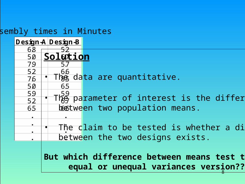
– Two samples are randomly and independently selected• A sample of 25 workers assembled a desk using design A. • A sample of 25 workers assembled the desk using design B.• The assembly times were recorded
– Do the assembly times of the two designs differs?
8
Design-A Design-B6.8 5.25.0 6.77.9 5.75.2 6.67.6 8.55.0 6.55.9 5.95.2 6.76.5 6.6. .. .. .. .
Design-A Design-B6.8 5.25.0 6.77.9 5.75.2 6.67.6 8.55.0 6.55.9 5.95.2 6.76.5 6.6. .. .. .. .
Assembly times in Minutes
Solution
• The data are quantitative.
• The parameter of interest is the difference between two population means.
• The claim to be tested is whether a difference between the two designs exists.
But which difference between means test to use?equal or unequal variances version???

9
F-Test Two-Sample for Variances
Method A Method BMean 6.288 6.016Variance 0.847766667 1.303066667Observations 25 25df 24 24F 0.650593472P(F<=f) one-tail 0.149605642F Critical one-tail 0.504092768
Method A Method B
Mean 6.288 Mean 6.016Standard Error 0.184148491 Standard Error 0.228304Median 6.3 Median 5.9Mode 5 Mode 5.9Standard Deviation 0.920742454 Standard Deviation 1.141519Sample Variance 0.847766667 Sample Variance 1.303067Kurtosis -0.760995145 Kurtosis -0.373591Skewness -0.095879182 Skewness 0.104214Range 3.3 Range 4.3Minimum 4.6 Minimum 4.2Maximum 7.9 Maximum 8.5Sum 157.2 Sum 150.4Count 25 Count 25Confidence Level(95.0%)0.380063727 Confidence Level(95.0%)0.471196

10
Design-A Design-B6.8 5.25.0 6.77.9 5.75.2 6.67.6 8.55.0 6.55.9 5.95.2 6.76.5 6.6. .. .. .. .
Design-A Design-B6.8 5.25.0 6.77.9 5.75.2 6.67.6 8.55.0 6.55.9 5.95.2 6.76.5 6.6. .. .. .. .
t-Test: Two-Sample Assuming Equal Variances
Design-A Design-BMean 6.288 6.016Variance 0.847766667 1.3030667Observations 25 25Pooled Variance 1.075416667Hypothesized Mean Difference0df 48t Stat 0.927332603P(T<=t) one-tail 0.179196744t Critical one-tail 1.677224191P(T<=t) two-tail 0.358393488t Critical two-tail 2.01063358
The Excel printout
P-value of the one tail test
P-value of the two tail test
Degrees of freedomt - statistic
2
1S 2
2S2
pS

11
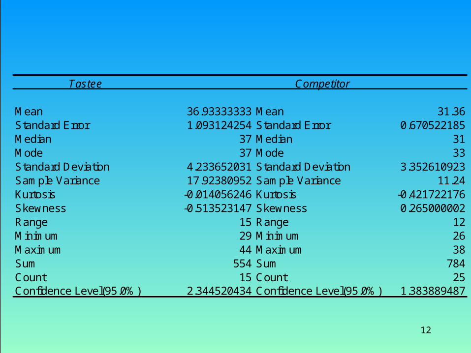
Example 12.23• The President of Tastee Inc., a baby-food producer, claims that his
company’s product is superior to that of his leading competitor, because babies gain weight faster with his product. To test this claim, a survey was undertaken. Mothers of newborn babies were asked which baby food they intended to feed their babies. Those who responded Tastee or the leading competitor were asked to keep track of their babies’ weight gains over the next two months. There were 15 mothers who indicated that they would feed their babies Tasteee and 25 who responded that they would feed their babies the product of the leading competitor. Each baby’s weight gain in ounces is recorded in XR12-23.
1. Can we conclude that, using weight gain as our criterion, Tastee baby food is indeed superior?
2. Estimate with 95% confidence the difference between the mean weight of the two products.
3. Check to ensure the required conditions are satisfied.
12
Tastee Competitor
Mean 36.93333333 Mean 31.36Standard Error 1.093124254 Standard Error 0.670522185Median 37 Median 31Mode 37 Mode 33Standard Deviation 4.233652031 Standard Deviation 3.352610923Sample Variance 17.92380952 Sample Variance 11.24Kurtosis -0.014056246 Kurtosis -0.421722176Skewness -0.513523147 Skewness 0.265000002Range 15 Range 12Minimum 29 Minimum 26Maximum 44 Maximum 38Sum 554 Sum 784Count 15 Count 25Confidence Level(95.0%) 2.344520434 Confidence Level(95.0%) 1.383889487

13
F-Test Two-Sample for Variances
Tastee CompetitorMean 36.93333333 31.36Variance 17.92380952 11.24Observations 15 25df 14 24F 1.594644975P(F<=f) one-tail 0.152491403F Critical one-tail 2.129795007
Example 12.23 (cont’d)

14
t-Test: Two-Sample Assuming Unequal Variances
Tastee CompetitorMean 36.93333333 31.36Variance 17.92380952 11.24Observations 15 25Hypothesized Mean Difference 0df 24t Stat 4.346056368P(T<=t) one-tail 0.000109546t Critical one-tail 1.710882316P(T<=t) two-tail 0.000219093t Critical two-tail 2.063898137
t-Test: Two-Sample Assuming Equal Variances
Tastee CompetitorMean 36.93333333 31.36Variance 17.92380952 11.24Observations 15 25Pooled Variance 13.70245614Hypothesized Mean Difference 0df 38t Stat 4.610005529P(T<=t) one-tail 2.22655E-05t Critical one-tail 1.685953066P(T<=t) two-tail 4.4531E-05t Critical two-tail 2.024394234

15
12.6 Inference about the difference between two population proportions• In this section we deal with two populations
whose data are qualitative.• When data are qualitative we can (only) ask
questions regarding the proportions of occurrence of certain outcomes.
• Thus, we hypothesize on the difference p1-p2, and draw an inference from the hypothesis test.

16
Sample 1 Sample size n1
Number of successes x1
Sample proportion
Sample 1 Sample size n1
Number of successes x1
Sample proportion
• Sampling Distribution of the Difference Between Two sample proportions
– Two random samples are drawn from two populations.– The number of successes in each sample is recorded.– The sample proportions are computed.
Sample 2 Sample size n2
Number of successes x2
Sample proportion
Sample 2 Sample size n2
Number of successes x2
Sample proportionx
n1
1
ˆ p1
2
22 n
xp̂
21 p̂p̂

17
– The statistic is approximately normally distributed if n1p1, n1(1 - p1), n2p2, n2(1 - p2) are all equal to or greater than 5.
– The mean of is p1 - p2.
– The variance of is p1(1-p1) /n1)+ (p2(1-p2)/n2)
21 p̂p̂
21 p̂p̂
21 p̂p̂
Because p1, p2, are unknown, we use their estimates instead. Thus, are all equal to or greater than 5.
22221111 q̂n,p̂n,q̂n,p̂n
ddistributenormallyelyapproximatis
n)p1(p
n)p1(p
)pp()p̂p̂(Z
statisticThe
2
22
1
11
2121
ddistributenormallyelyapproximatis
n)p1(p
n)p1(p
)pp()p̂p̂(Z
statisticThe
2
22
1
11
2121

18
• Testing the Difference between Two Population Proportions
– We hypothesize on the difference between the two proportions, p1 - p2.
– There are two cases to consider:
21 pp
Case 1: H0: p1-p2 =0
Calculate the pooled proportion
21
21
nn
xxp̂
Then Then
Case 2: H0: p1-p2 =D (D is not equal to 0)Do not pool the data
2
22 n
xp̂
1
11 n
xp̂
)n1
n1
)(p̂1(p̂
)pp()p̂p̂(Z
21
2121
)n1
n1
)(p̂1(p̂
)pp()p̂p̂(Z
21
2121
2
22
1
11
21
n)p̂1(p̂
n)p̂1(p̂
D)p̂p̂(Z
2
22
1
11
21
n)p̂1(p̂
n)p̂1(p̂
D)p̂p̂(Z

19
• Example 12.7– A research project employing 22,000 American
physicians was conduct to discover whether aspirin can prevent heart attacks.
– Half of the participants in the research took aspirin, and half took placebo.
– In a three years period,104 of those who took aspirin and 189 of those who took the placebo had had heart attacks.
– Is aspirin effective in preventing heart attacks?
20
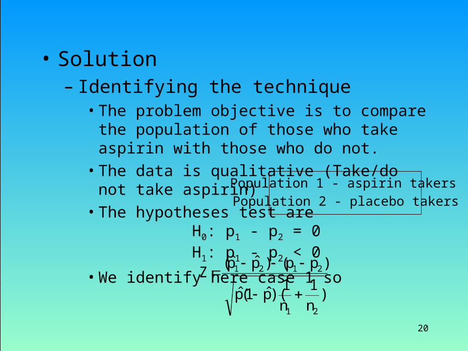
• Solution– Identifying the technique
• The problem objective is to compare the population of those who take aspirin with those who do not.
• The data is qualitative (Take/do not take aspirin)• The hypotheses test are
H0: p1 - p2 = 0H1: p1 - p2 < 0
• We identify here case 1 so
)n1
n1
)(p̂1(p̂
)pp()p̂p̂(Z
21
2121
Population 1 - aspirin takersPopulation 2 - placebo takers

21
– Solving by hand• For a 5% significance level the rejection region is
z < -z = -z.05 = -1.645
01718.000,11189p̂and,00945.000,11104p̂
aresproportionsampleThe
21
01332.)000,11000,11()189104()()(ˆ 2121 nnxxp
isproportionpooledThe
02.5)
000,111
000,111
)(98668(.01332.
01718.009455.
)n1
n1
)(p̂1(p̂
)pp()p̂p̂(Z
becomesstatisticzThe
21
2121
- 5.02 < - 1.645, so rejectthe null hypothesis.

22
• Example 12.59– Random samples from two binomial populations
yielded the following statistics= .45 n1=100 =.39 n2=100
– Test with alpha = 0.10 to determine whether we can infer that the population proportions differ.
1p̂ 2p̂

23
• Example 12.66– The following statistics were calculated
= .12 n1=400 =.16 n2=400
– Test with alpha = 0.10 to determine whether p1 is less than p2.
1p̂ 2p̂

24
• Example 12.64– After sampling two binomial populations we found
the following.= .368 n1=100 =.275 n2=1000
– Can we infer at the 5% significance level that p1 is greater than p2 by more than 5%?
1p̂ 2p̂