echem user’s guide - san diego miramar...
TRANSCRIPT

PowerLab
®
System
www.
ADInstruments
.com
V E R S I O N 1 . 5
EChemUser’s Guide
& using Chart & Scope software for Electrochemistry

ii
EChem User’s Guide
This document was, as far as possible, accurate at the time of printing. Changes may have been made to the software and hardware it describes since then, though: ADInstruments Pty Ltd reserves the right to alter specifications as required. Late-breaking information may be supplied separately.
Trademarks of ADInstruments
MacLab and PowerLab are registered trademarks of ADInstruments Pty Ltd. Specific model names of data recording units, such as MacLab/8e and PowerLab/400, are trademarks of ADInstruments Pty Ltd.
Chart, EChem, Histogram, Peaks, Scope, DoseResponse, UpdateMaker, and UpdateUser (software), and PowerChrom (software and hardware) are trademarks of ADInstruments Pty Ltd.
Other Trademarks
Apple, the Apple logo, AppleTalk, Geneva, HyperCard, ImageWriter, LaserWriter, Macintosh, and StyleWriter are registered trademarks of Apple Computer, Inc. Finder, MacOS, Power Macintosh PowerBook, PowerTalk, Quadra, QuickDraw, System 7, and TrueType are trademarks of Apple Computer, Inc. Windows, Windows 95, Windows 98 and Windows NT are trademarks of Microsoft Corporation..
PostScript is a registered trademark of Adobe Systems, Incorporated.
BAS is a trademark of Bioanalytical Systems Inc. PAR and EG&G PARC are trademarks of EG&G Princeton Applied Reasearch. Polarecord is a trademark of Metrohm Ltd. HEKA is a trademark of HEKA Electronik. PINE is a trademark of PINE Instrument Company. Cypress is a trademark of Cypress Systems Inc. AMEL is a trademark of AMEL srl.
I
GOR &
I
GOR Pro (software) are trademarks of Wavemetrics Inc.
EChem 1.3 software: Michael Macknight, Peter Bromley, Bruce Warrington, and Michael Hamel.
EChem 1.5 software written byLev Possajennikov.
Documentation written by Paul Duckworth.
Document Number: U-MS600-UG-03ACopyright © July 1999ADInstruments Pty LtdUnit 6, 4 Gladstone RoadCastle Hill, NSW 2154AUSTRALIA
e-mail: [email protected]://www.adinstruments.com
All rights reserved. No part of this document may be reproduced by any means without the prior written permission of ADInstruments Pty Ltd.
EChem
3 Se
UsingCoAdUsUn
The AChTh
4 Da
The M
Contents
Contents iii
1 Getting Started 1
Learning to Use EChem 2Computer Requirements 3The EChem System 4Installation Instructions 6Opening EChem for the first time 6
2 EChem Basics 9
An Overview of EChem 10Opening an EChem File 12Closing or Quitting an EChem File 14The Main Window 14Recording 19
The Axes 40Dragging and Stretching the Axes 42Graph Lines, Patterns & Colors 43Navigating 44Overlaying Pages 45The Zoom Window 47Display and Printer Resolution 49Making Measurements 50
Using the Marker 50Setting and Removing Baselines 51The Marker Miniwindow 52
Background Subtraction 54The Data Pad 55
Adding Data to the Data Pad 57Setting Up the Columns 57Data Pad Miniwindow 59Printing the Data Pad 59
Computed Functions 59
User’s Guide iii
tting Up EChem 23
3rd Party Potentiostats 24nnecting to PowerLab 24justing the Input Range 25ing the Input Amplifier Dialog Box 26its Conversion 29DInstruments Potentiostat 31anging Potentiostat settings 31e Potentiostat Dialog Box 31
ta Display and Analysis 37
ain EChem Window 38
Sampling Speed 60Channel Functions 61Math 62Function 63
The Notebook 64The Page Comment window 65
5 Working With Files 67
Selecting Data 68Editing Data 68Transferring Data 69Measuring From the Waveform 71
Using the Marker 72
Setting and Removing Baselines 73Saving Options 74Appending Files 77Text Files 77Printing 79
Page Setup 80The Print Command 82
6 Customizing EChem
87
Preferences 88Menus 88Controls 90Options 91Start-Up 92Emergency Access! 92
Macros 94Recording a Macro 95Playing a Macro 96Deleting a Macro 96Macros That Call Other Macros 97Options When Recording Macros 98Macro Commands 101
7 EChem Techniques
107
Introduction 108General Considerations 110Linear Sweep Voltammetry 116Square Wave Voltammetry 121Normal Pulse Voltammetry 126Differential Pulse Voltammetry 130Stripping Techniques 135
Chronocoulometry 173Chronopotentiometry 175The Potentiostat as a Galvanostat 175Controlled Potential Electrolysis 178Controlled Current Electrolysis 179Rotating Ring Disk Electrodes 180Amperometric Titrimetry 180Liquid Chromatography Detectors 181Biosensors 182Potentiometric sensors 182
pH Electrodes 182Ion Selective Electrodes 183Potentiometric Redox Electrodes 184Dissolved CO
2
and NH
3
Electrodes 184Electrode Behaviour 184Multiple Point Calibration 185pH and ISE Calibration 189Temperature Compensation 194Isopotential Point 196
Potentiometric Titrimetry 197Dissolved Oxygen, dO2, Sensors 198Conductivity Sensors 198Simple Galvanic Cells 199Quartz Crystal Microbalance 200Electrochemical Noise Experiments 200Corrosion Measurements 201
9 Using 3rd Party Equipment
205
Introduction 206EG&G PARC 206BAS
210PINE
214
iv EChem User’s Guide
Cyclic Voltammetry 140MultiPulse Voltammetry 146MultiPulse Amperometry 154The Apply Technique... command 159Polarographic Techniques 160
8 Additional Techniques 161
Introduction 162AC Voltammetry 163Fast Scan Techniques 163Low Current Experiments 166Chronoamperometry 167
Metrohm 215Schlumberger 216Radiometer 216HEKA 217Cypress 218AMEL 220

Appendices
A Menus & Commands
223
Menus 223Keyboard Shortcuts 226
B Troubleshooting
227
Technical Support 227Solutions to Common Problems 229
C Technique Summary
241
Linear Sweep Voltammetry 242Square Wave Voltammetry 243Normal & Reverse Pulse Voltammetry 244Differential Pulse Voltammetry 245Cyclic Voltammetry 246Multi Pulse Voltammetry 247
D Electrochemical Equations
249
Linear Sweep and Cyclic Voltammetry, The Randles-Sevcik Equation 249Differential Pulse Techniques, The Parry-Osteryoung Equation 251Chronoamperometry, The Cottrell
Chapter — Contents v
Equation 252Chronocoulometry, The Integrated Cottrell Equation 253
E Cyclic Voltammetry, Solvents & Electrolytes 255
Solubility Rules 255Solvent Stability 256Use of Large Ions as Electrolytes 256Electrode and Cell Design for Organic Solvents 259Synthesis of Selected Electrolytes 261
Purification of solvents 264Supercritical Fluids 265The Mercury Electrode 265
F Potentiostat Designs 267
Two electrode systems 267Three electrode systems 268Four electrode systems 270
Bibliography 273
The Internet 273Text Books 274Journals 279
Glossary 281
Index 285
Licensing & Warranty Agreement 295

vi EChem User’s Guide
EChem
User’s Guide
1
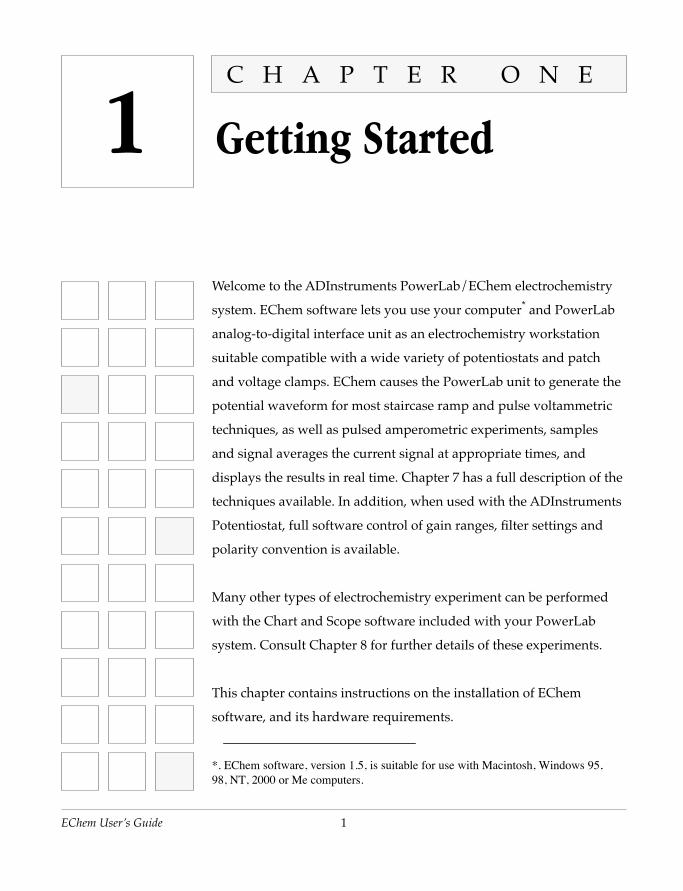
C H A P T E R O N E
Getting Started
Welcome to the ADInstruments PowerLab/EChem electrochemistry
system. EChem software lets you use your computer* and PowerLab
analog-to-digital interface unit as an electrochemistry workstation
suitable compatible with a wide variety of potentiostats and patch
and voltage clamps. EChem causes the PowerLab unit to generate the
potential waveform for most staircase ramp and pulse voltammetric
techniques, as well as pulsed amperometric experiments, samples
and signal averages the current signal at appropriate times, and
displays the results in real time. Chapter 7 has a full description of the
techniques available. In addition, when used with the ADInstruments
Potentiostat, full software control of gain ranges, filter settings and
polarity convention is available.
1
Many other types of electrochemistry experiment can be performed
with the Chart and Scope software included with your PowerLab
system. Consult Chapter 8 for further details of these experiments.
This chapter contains instructions on the installation of EChem
software, and its hardware requirements.
*. EChem software, version 1.5, is suitable for use with Macintosh, Windows 95,98, NT, 2000 or Me computers.

2
Learning to Use
E
Chem
Where to Start
To install and use EChem you should be familiar with the operating system of your computer.
You will find that EChem works similarly to other programs that you use on your computer. If you have used earlier versions of EChem software, you should find that although this version has much in common, it also has many new features.
Start by reading the introductory chapters in your
Getting Started with PowerLab
booklet
which describes how to connect the PowerLab unit to your computer. If you are not using an ADInstruments Potentiostat then you should also read Chapter 9 before using the system. If you are new to electrochemical techniques, then first familiarise yourself with the various terms defined in the Glossary at the end of this guide.
How to Use this Guide
If you are in a hurry at least read the rest of this chapter, and the Overview of EChem in the next chapter, to familiarise yourself with some of the key features of EChem before you begin your experiments.
We recommend, however, that you work through this guide in front
EChem User’s Guide
of your computer. The information in the following chapters is set out in the order you will probably require it. If you are unfamiliar with electrochemical methods then read Chapters 7 and 8. The appendices also have much useful information including electrolyte syntheses, solvent purification methods, and sources of general information.
The rest of this chapter, covers system configurations and installing and personalising your copy of EChem.
If you are using a third party potentiostat with EChem then please read the potentiostat operator’s manual carefully to determine its limitations safe operating procedure. In particular be aware of the
Chapter 1 — Getting Starte
NoteOwners of Apple Macintosh PowerBooks will need a suitable SCSI cable or adaptor, available from your computer dealer, to connect the PowerBook to the PowerLab unit. Recent Macintosh models have a USB port which can be used as an alternative to the SCSI connection with PowerLab units with USB ports.
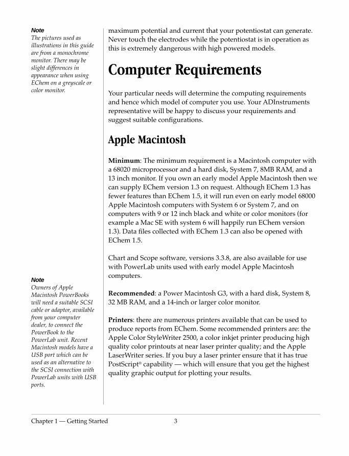
Note The pictures used as illustrations in this guide are from a monochrome monitor. There may be slight differences in appearance when using EChem on a greyscale or color monitor.
maximum potential and current that your potentiostat can generate. Never touch the electrodes while the potentiostat is in operation as this is extremely dangerous with high powered models.
Computer Requirements
Your particular needs will determine the computing requirements and hence which model of computer you use. Your ADInstruments representative will be happy to discuss your requirements and suggest suitable configurations.
Apple Macintosh
Minimum
: The minimum requirement is a Macintosh computer with a 68020 microprocessor and a hard disk, System 7, 8MB RAM, and a 13 inch monitor. If you own an early model Apple Macintosh then we can supply EChem version 1.3 on request. Although EChem 1.3 has fewer features than EChem 1.5, it will run even on early model 68000 Apple Macintosh computers with System 6 or System 7, and on computers with 9 or 12 inch black and white or color monitors (for example a Mac SE with system 6 will happily run EChem version 1.3). Data files collected with EChem 1.3 can also be opened with EChem 1.5.
Chart and Scope software, versions 3.3.8, are also available for use with PowerLab units used with early model Apple Macintosh computers.
d 3
Recommended: a Power Macintosh G3, with a hard disk, System 8, 32 MB RAM, and a 14-inch or larger color monitor.
Printers: there are numerous printers available that can be used to produce reports from EChem. Some recommended printers are: the Apple Color StyleWriter 2500, a color inkjet printer producing high quality color printouts at near laser printer quality; and the Apple LaserWriter series. If you buy a laser printer ensure that it has true PostScript® capability — which will ensure that you get the highest quality graphic output for plotting your results.
4
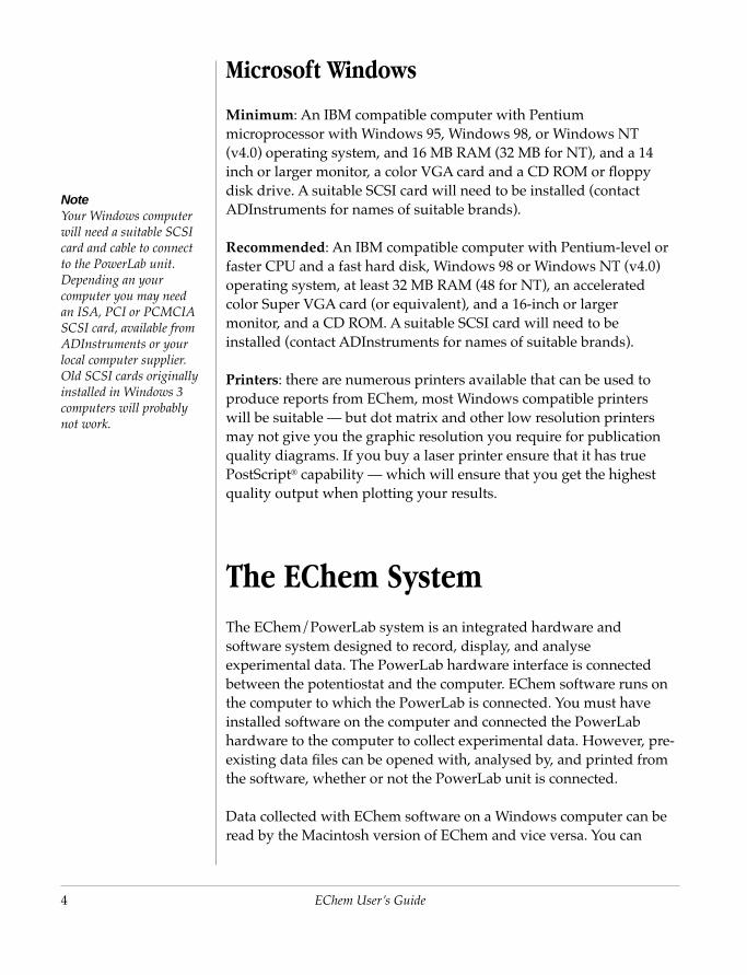
NoteYour Windows computer will need a suitable SCSI card and cable to connect to the PowerLab unit. Depending an your computer you may need an ISA, PCI or PCMCIA SCSI card, available from ADInstruments or your local computer supplier. Old SCSI cards originally installed in Windows 3 computers will probably not work.
Microsoft Windows
Minimum
: An IBM compatible computer with Pentium microprocessor with Windows 95, Windows 98, or Windows NT (v4.0) operating system, and 16 MB RAM (32 MB for NT), and a 14 inch or larger monitor, a color VGA card and a CD ROM or floppy disk drive. A suitable SCSI card will need to be installed (contact ADInstruments for names of suitable brands).
Recommended
: An IBM compatible computer with Pentium-level or faster CPU and a fast hard disk, Windows 98 or Windows NT (v4.0) operating system, at least 32 MB RAM (48 for NT), an accelerated color Super VGA card (or equivalent), and a 16-inch or larger monitor, and a CD ROM. A suitable SCSI card will need to be installed (contact ADInstruments for names of suitable brands).
Printers
: there are numerous printers available that can be used to produce reports from EChem, most Windows compatible printers will be suitable — but dot matrix and other low resolution printers may not give you the graphic resolution you require for publication quality diagrams. If you buy a laser printer ensure that it has true PostScript
®
capability — which will ensure that you get the highest quality output when plotting your results.
The EChem System
EChem User’s Guide
The EChem/PowerLab system is an integrated hardware and software system designed to record, display, and analyse experimental data. The PowerLab hardware interface is connected between the potentiostat and the computer. EChem software runs on the computer to which the PowerLab is connected. You must have installed software on the computer and connected the PowerLab hardware to the computer to collect experimental data. However, pre-existing data files can be opened with, analysed by, and printed from the software, whether or not the PowerLab unit is connected.
Data collected with EChem software on a Windows computer can be read by the Macintosh version of EChem and vice versa. You can
Chapter 1 — Getting Starte
transfer data between computers on Windows formatted floppy disks (Macintosh computers read Windows formatted disks).
Other ADinstruments software that runs with PowerLab units, includes Chart and Scope software (supplied with the PowerLab unit). Other software that can be used with your PowerLab hardware is available separately and includes PowerChrom software (for chromatographic data collection), and DoseResponse software (for pharmacological studies).
Compatible MacLab or PowerLab Units
EChem 1.5 software can be used with the following new and older models of PowerLab and MacLab.
PowerLab e systems:
•PowerLab/200, MacLab/200, MacLab/2e
•PowerLab/400, MacLab/400, MacLab/4e, MacLab/4
•PowerLab/800, MacLab/8e, MacLab/8
PowerLab S systems:
•PowerLab/4
SP
, PowerLab/4s, MacLab/4s
•PowerLab/8
SP
, PowerLab/8s, MacLab/8s
•PowerLab/16
SP
, PowerLab/16s, MacLab/16s
•PowerLab/4
ST
d 5
The PowerLab/410 is unsuitable for use with EChem software. Consult your ADInstruments representative for the latest information on our range of products. Please note that MacLab units have now been superseded by the PowerLab range.
Optional Analysis
For general purpose data analysis and the production of specialist plots for theses, reports, slides, and publications we recommend IGOR Pro software (WaveMetrics). Other suitable graphing software includes Origin (Microcal) and Kaleidagraph (Synergy).
6
Figure 1–1
The EChem program icon
Installation InstructionsYou will have been provided with a CD ROM which contains the EChem installer software. If your computer does not have CD ROM capability then contact your ADInstruments representative who can arrange installation from a set of floppy disks. You will need at least 3 MB of free space on your hard disk for the installation. It is recommended that you first install the Chart and Scope software that also came with your PowerLab system. To install EChem:
1. Insert the EChem PowerLab CD ROM into the appropriate drive.
2. Double click the installer icon.
The installation creates an EChem folder (directory) in which you will find the EChem program and sample data files. On Macintosh systems the ‘Potentiostat’ driver software is also placed in the ‘ADInstruments’ folder in the System Folder. On a Windows system the Potentiostat driver is part of the EChem software. This driver is only required if you are using the ADInstruments Potentiostat.
If you have used an earlier version of EChem it is strongly recommended that you remove these versions from your Macintosh hard disk before you install EChem 1.5. On Windows systems older versions of software will be automatically uninstalled. Data files from earlier versions of EChem will open with EChem version 1.5. If there are multiple versions of a program present on your hard disk then you may accidentally use the older version for your experiments.
Keep your installer CD ROM in a safe place after the installation.
EChem User’s Guide
Please remember that each purchased copy only licenses you to use the software on one computer at any one time. Please enquire about a cost–saving departmental license if you want to run multiple copies in your workplace.
Opening EChem for the first timeEnsure that the PowerLab unit is connected properly to your computer (this is covered in the Owner’s Guide that came with your PowerLab unit), and that it is turned on. Click the EChem icon and select Open from the File menu (or double-click the icon). There may be a short delay while the program initialises the PowerLab unit.
Chapter 1 — Getting Starte
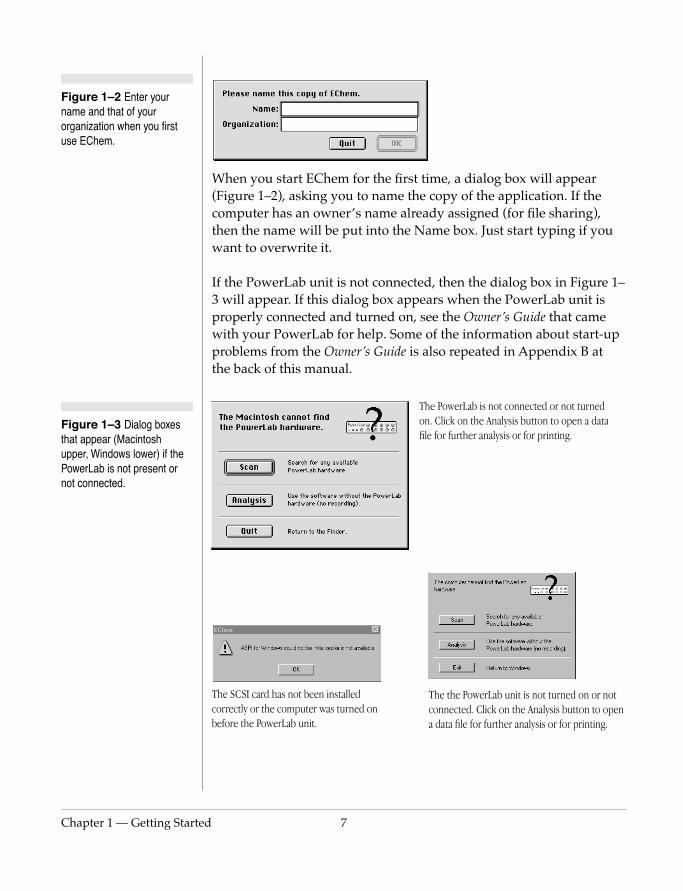
Figure 1–3 Dialog boxes that appear (Macintosh upper, Windows lower) if the PowerLab is not present or not connected.
Figure 1–2 Enter your name and that of your organization when you first use EChem.
When you start EChem for the first time, a dialog box will appear (Figure 1–2), asking you to name the copy of the application. If the computer has an owner’s name already assigned (for file sharing), then the name will be put into the Name box. Just start typing if you want to overwrite it.
If the PowerLab unit is not connected, then the dialog box in Figure 1–3 will appear. If this dialog box appears when the PowerLab unit is properly connected and turned on, see the
Owner’s Guide
that came with your PowerLab for help. Some of the information about start-up problems from the Owner’s Guide is also repeated in Appendix B at the back of this manual.
The PowerLab is not connected or not turned on. Click on the Analysis button to open a data file for further analysis or for printing.
d 7
The SCSI card has not been installed correctly or the computer was turned on before the PowerLab unit.
The the PowerLab unit is not turned on or not connected. Click on the Analysis button to open a data file for further analysis or for printing.

8
Quitting EChem
If you want to exit EChem after naming your copy of the software, choose Quit from the File menu. If you want to proceed, working through this guide, you can leave the file open.
EChem User’s Guide

EChem
User’s Guide2
C H A P T E R T W OEChem Basics
EChem is a sophisticated program for performing voltammetric and
amperometric electrochemical experiments. This chapter provides a
general overview of EChem, looks at the main graphic window, and
deals with the basics of recording data.
9
10
An Overview of EChemEChem, together with the PowerLab hardware and computer, gives you the display capabilities of a two-channel storage oscilloscope, as well as the features of a versatile waveform generator. You can perform a variety of electrochemical techniques with any potentiostat that has an external input and analog (XY, or chart recorder) outputs.
Display Controls—Chapter 4
Your results are displayed in the main EChem window which can be resized, and the control panels moved to where you want them. The data display can be set to show I (current), E (potential) and t (time) in different formats:
• I vs E, with I on the Y and E on the X axis.
• E vs I, with E on the Y axis and I on the X axis.
• I and E on separate graphs versus time.
• I versus time (for amperometric experiments).
The current and potential axes can be dragged, stretched, or set to exact values for optimum data display. The current range can be adjusted. If an ADInstruments Potentiostat is connected then its controls can also be accessed through the software. Display colors, patterns, and grids can be altered.
Display and Analysis—Chapter 4
EChem User’s Guide
EChem records data in sweeps, like a normal oscilloscope, however each new sweep is recorded to a different ‘page’, creating a set of recorded scans numbered for easy reference, or for overlaying. Thus a new file does not have to be created for each experiment. You can add your own written comments to each ‘page’ of data to emphasize features of interest, or to log standard concentrations. There is also a Notebook feature for making general observations about a data file.
When you have finished recording, you can move through your data using the page controls and make measurements directly from the recording — you are given a direct read-out, with no chance of
Chapter 2 — EChem Basic
measurement errors. You can measure from a selected reference point, using the Marker, or a baseline (which you can also set). EChem allows you to overlay data from any selection of pages, for direct comparison. The Data Pad feature enables you to make and store parameters such as peak height, potential at peak height, etc. EChem has a Zoom window for examining a section of the recording in more detail. Refer to Chapter 5 for more details.
Working with Files—Chapter 5
EChem results can be printed, edited, and saved to a disk for later review. You can also save ‘settings files’ — empty data files that are preconfigured for particular experiments — so that any experiment can be repeated quickly and easily, without having to go through the process of entering all the sweep parameters again. Pages of data can be printed in a variety of formats, or cut, copied, and pasted between EChem files, and whole files can be appended to the end of an open file, allowing you to produce summaries in a single file. Data can be transferred as text to spreadsheets or word processors and, conversely, correctly formatted text can even be pasted into an EChem file.
Techniques— Chapters 7 and 8
EChem provides a range of electrochemical methods from simple staircase linear sweep voltammetry through to complicated pulse sequences. You can define the sampling periods for each step or pulse.
Customising and Automating— Chapter 6
s 11
EChem can be extensively customised for your purposes. Controls, and menus and their commands (and Command-key/Control-key equivalents) can be locked, hidden, or altered, and the appearance of EChem simplified, say, for student or technician use. Macros can also be created to automate complex, or repetitive tasks.
12
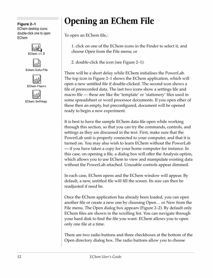
Figure 2–1EChem desktop icons: double-click one to open EChem
Opening an EChem FileTo open an EChem file,:
1. click on one of the EChem icons in the Finder to select it, and choose Open from the File menu; or
2. double-click the icon (see Figure 2–1).
There will be a short delay while EChem initialises the PowerLab. The top icon in Figure 2–1 shows the EChem application, which will open a new untitled file if double-clicked. The second icon shows a file of prerecorded data. The last two icons show a settings file and macro file — these are like the ‘template’ or ‘stationery’ files used in some spreadsheet or word processor documents. If you open ether of these then an empty, but preconfigured, document will be opened ready to begin a new experiment.
It is best to have the sample EChem data file open while working through this section, so that you can try the commands, controls, and settings as they are discussed in the text. First, make sure that the PowerLab unit is properly connected to your computer, and that it is turned on. You may also wish to learn EChem without the PowerLab — if you have taken a copy for your home computer for instance. In this case, on opening a file, a dialog box will offer the Analysis option, which allows you to use EChem to view and manipulate existing data without the PowerLab attached. Unusable controls appear dimmed.
In each case, EChem opens and the EChem window will appear. By
EChem User’s Guide
default, a new, untitled file will fill the screen. Its size can then be readjusted if need be.
Once the EChem application has already been loaded, you can open another file or create a new one by choosing Open… or New from the File menu. The Open dialog box appears (Figure 2–2). By default only EChem files are shown in the scrolling list. You can navigate through your hard disk to find the file you want. EChem allows you to open only one file at a time.
There are two radio buttons and three checkboxes at the bottom of the Open directory dialog box. The radio buttons allow you to choose
Chapter 2 — EChem Basic
NoteTo start EChem with its factory default settings, hold down the Command key (Macintosh) or Control key (PC) immediately after you start the software by double-clicking the icon. Release the key when the alert box appears, and click the OK button.
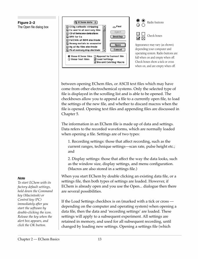
Figure 2–2 The Open file dialog box
between opening EChem files, or ASCII text files which may have come from other electrochemical systems. Only the selected type of file is displayed in the scrolling list and is able to be opened. The checkboxes allow you to append a file to a currently open file, to load the settings of the new file, and whether to discard macros when the file is opened. Opening text files and appending files are discussed in Chapter 5.
The information in an EChem file is made up of data and settings. Data refers to the recorded waveforms, which are normally loaded when opening a file. Settings are of two types:
1. Recording settings: those that affect recording, such as the current ranges, technique settings—scan rate, pulse height etc.; and
2. Display settings: those that affect the way the data looks, such as the window size, display settings, and menu configuration.
Radio buttons
Check boxes
Appearance may vary (as shown) depending your computer and operating system. Radio buttons are full when on and empty when off. Check boxes show a tick or cross when on, and are empty when off.
s 13
(Macros are also stored in a settings file.)
When you start EChem by double clicking an existing data file, or a settings file, then both types of settings are loaded. However, if EChem is already open and you use the Open... dialogue then there are several possibilities.
If the Load Settings checkbox is on (marked with a tick or cross — depending on the computer and operating system) when opening a data file, then the data and ‘recording settings’ are loaded. These settings will apply to a subsequent experiment. All settings are retained in memory, and used for all subsequent recording, until changed by loading new settings. Opening a settings file (which

14
contains no data) with the Load Settings checkbox off will load only display settings, not those affecting recording of data.
If you have a file open when opening a second file, then the first file will be closed. If there are any unsaved changes to the first file, an alert box will appear asking if you want to save them before opening the new file. If the Load Settings checkbox is on, then both the settings and the data will be loaded, otherwise the current settings from the first file are retained.
Using the sample data file as you work through this user’s guide will show you some real data and perhaps give a better idea of what is going on in EChem.
Closing or Quitting an EChem File
To close an EChem file, choose Close from the File menu or click in the close box in the Main window (upper left corner, Figure 2–3). To quit EChem, choose Quit from the File menu. In either case, if you have made any changes, a dialog box will appear, asking you if you wish to save your work. Click the Save button if you wish to keep the changes you have made. Click the Don’t Save button if you want to discard the changes.
The Main WindowThe essential controls for recording data are provided in the Main window and its various control panels, illustrated in Figure 2–3.
EChem User’s Guide
These controls are discussed below, and in greater detail elsewhere in this manual. The window itself consists of, the data display area, which contains recorded data; and some controls at the bottom of the window. Various movable control panels surround the window proper. The menu bar at the top of the screen contains the EChem menus (see Appendix A), allowing you to set up and modify the way EChem looks and behaves. The EChem Window command from the Windows menu returns to this window from another, or opens a new, untitled file if the window has been closed.
Chapter 2 — EChem Basic
Close box
Ti
Scale pop-up menu
Axis label
Display pop(i vs E displa
Page
Marker
Page Comment button
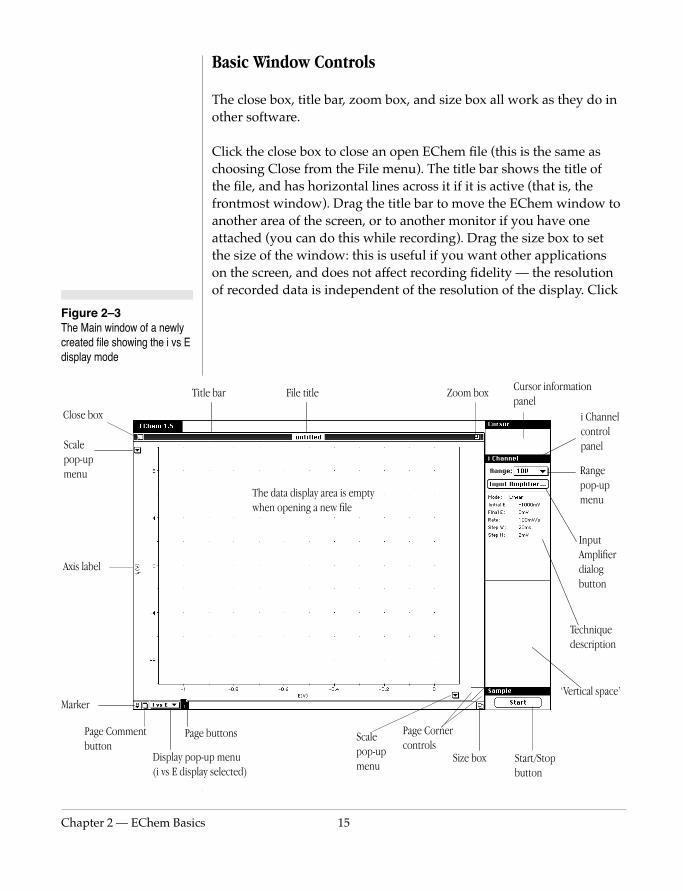
Figure 2–3 The Main window of a newly created file showing the i vs E display mode
Basic Window Controls
The close box, title bar, zoom box, and size box all work as they do in
other software.Click the close box to close an open EChem file (this is the same as
s 15
choosing Close from the File menu). The title bar shows the title of the file, and has horizontal lines across it if it is active (that is, the frontmost window). Drag the title bar to move the EChem window to another area of the screen, or to another monitor if you have one attached (you can do this while recording). Drag the size box to set the size of the window: this is useful if you want other applications on the screen, and does not affect recording fidelity — the resolution of recorded data is independent of the resolution of the display. Click
tle bar File title Zoom box
The data display area is empty when opening a new file
-up menu y selected)
buttons
Size box
Cursor information panel
Range pop-up menu
Input Amplifier dialog button
Start/Stop button
i Channel control panel
Technique description
Scale pop-up menu
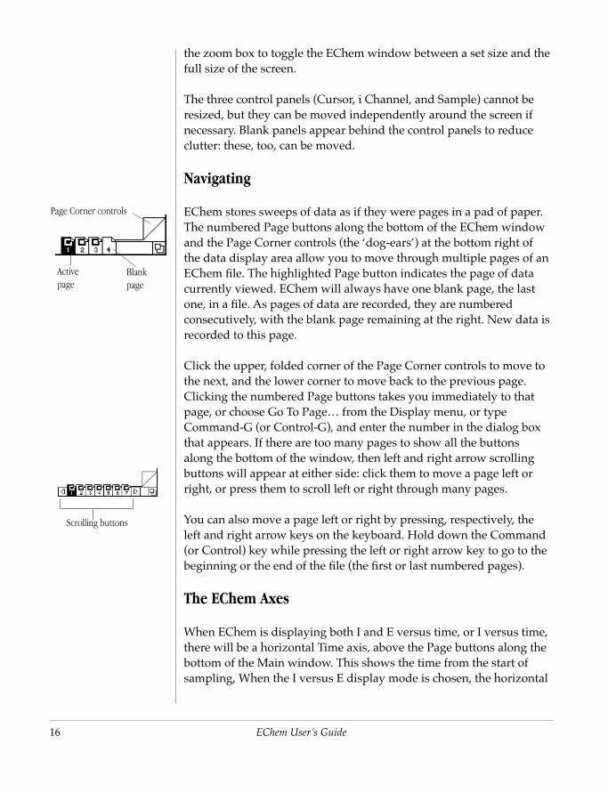
Page Corner controls
‘Vertical space’
16
Scrolling buttons
Blank page
Active page
Page Corner controls
the zoom box to toggle the EChem window between a set size and the full size of the screen.
The three control panels (Cursor, i Channel, and Sample) cannot be resized, but they can be moved independently around the screen if necessary. Blank panels appear behind the control panels to reduce clutter: these, too, can be moved.
Navigating
EChem stores sweeps of data as if they were pages in a pad of paper. The numbered Page buttons along the bottom of the EChem window and the Page Corner controls (the ‘dog-ears’) at the bottom right of the data display area allow you to move through multiple pages of an EChem file. The highlighted Page button indicates the page of data currently viewed. EChem will always have one blank page, the last one, in a file. As pages of data are recorded, they are numbered consecutively, with the blank page remaining at the right. New data is recorded to this page.
Click the upper, folded corner of the Page Corner controls to move to the next, and the lower corner to move back to the previous page. Clicking the numbered Page buttons takes you immediately to that page, or choose Go To Page… from the Display menu, or type Command-G (or Control-G), and enter the number in the dialog box that appears. If there are too many pages to show all the buttons along the bottom of the window, then left and right arrow scrolling buttons will appear at either side: click them to move a page left or right, or press them to scroll left or right through many pages.
EChem User’s Guide
You can also move a page left or right by pressing, respectively, the left and right arrow keys on the keyboard. Hold down the Command (or Control) key while pressing the left or right arrow key to go to the beginning or the end of the file (the first or last numbered pages).
The EChem Axes
When EChem is displaying both I and E versus time, or I versus time, there will be a horizontal Time axis, above the Page buttons along the bottom of the Main window. This shows the time from the start of sampling, When the I versus E display mode is chosen, the horizontal
Chapter 2 — EChem Basic
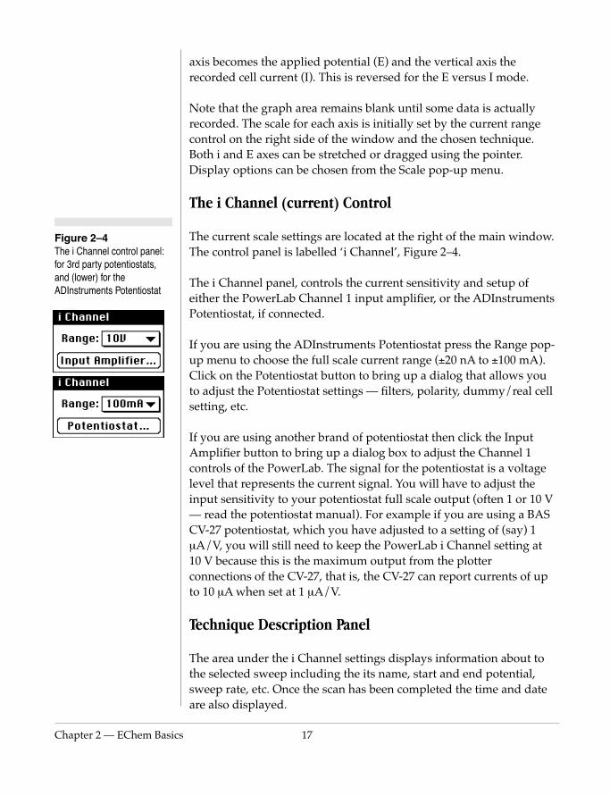
Figure 2–4 The i Channel control panel: for 3rd party potentiostats, and (lower) for the ADInstruments Potentiostat
axis becomes the applied potential (E) and the vertical axis the recorded cell current (I). This is reversed for the E versus I mode.
Note that the graph area remains blank until some data is actually recorded. The scale for each axis is initially set by the current range control on the right side of the window and the chosen technique. Both i and E axes can be stretched or dragged using the pointer. Display options can be chosen from the Scale pop-up menu.
The i Channel (current) Control
The current scale settings are located at the right of the main window. The control panel is labelled ‘i Channel’, Figure 2–4.
The i Channel panel, controls the current sensitivity and setup of either the PowerLab Channel 1 input amplifier, or the ADInstruments Potentiostat, if connected.
If you are using the ADInstruments Potentiostat press the Range pop-up menu to choose the full scale current range (±20 nA to ±100 mA). Click on the Potentiostat button to bring up a dialog that allows you to adjust the Potentiostat settings — filters, polarity, dummy/real cell setting, etc.
If you are using another brand of potentiostat then click the Input Amplifier button to bring up a dialog box to adjust the Channel 1 controls of the PowerLab. The signal for the potentiostat is a voltage level that represents the current signal. You will have to adjust the input sensitivity to your potentiostat full scale output (often 1 or 10 V — read the potentiostat manual). For example if you are using a BAS
s 17
CV-27 potentiostat, which you have adjusted to a setting of (say) 1 µA/V, you will still need to keep the PowerLab i Channel setting at 10 V because this is the maximum output from the plotter connections of the CV-27, that is, the CV-27 can report currents of up to 10 µA when set at 1 µA/V.
Technique Description Panel
The area under the i Channel settings displays information about to the selected sweep including the its name, start and end potential, sweep rate, etc. Once the scan has been completed the time and date are also displayed.
18
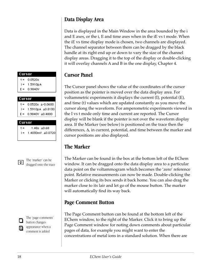
The ‘page comments’ button changes appearance when a comment is added
The ‘marker’ can be dragged onto the trace
Data Display Area
Data is displayed in the Main Window in the area bounded by the i and E axes, or the i, E and time axes when in the iE vs t mode. When the iE vs time display mode is chosen, two channels are displayed. The channel separator between them can be dragged by the black handle at its right end up or down to vary the size of the channel display areas. Dragging it to the top of the display or double-clicking it will overlay channels A and B in the one display, Chapter 4.
Cursor Panel
The Cursor panel shows the value of the coordinates of the cursor position as the pointer is moved over the data display area. For voltammetric experiments it displays the current (I), potential (E), and time (t) values which are updated constantly as you move the cursor along the waveform. For amperometric experiments viewed in the I vs t mode only time and current are reported. The Cursor display will be blank if the pointer is not over the waveform display area. If the Marker (see below) is positioned on the trace then the differences, ∆, in current, potential, and time between the marker and cursor positions are also displayed.
The Marker
The Marker can be found in the box at the bottom left of the EChem window. It can be dragged onto the data display area to a particular data point on the voltammogram which becomes the ‘zero’ reference point. Relative measurements can now be made. Double-clicking the
EChem User’s Guide
Marker or clicking its box sends it back home. You can also drag the marker close to its lair and let go of the mouse button. The marker will automatically find its way back.
Page Comment Button
The Page Comment button can be found at the bottom left of the EChem window, to the right of the Marker. Click it to bring up the Page Comment window for noting down comments about particular pages of data, for example you might want to enter the concentrations of metal ions in a standard solution. When there are
Chapter 2 — EChem Basic
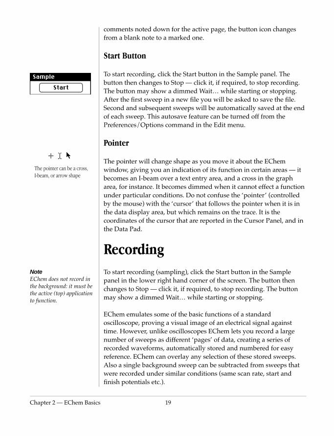
The pointer can be a cross, I-beam, or arrow shape
NoteEChem does not record in the background: it must be the active (top) application to function.
comments noted down for the active page, the button icon changes from a blank note to a marked one.
Start Button
To start recording, click the Start button in the Sample panel. The button then changes to Stop — click it, if required, to stop recording. The button may show a dimmed Wait… while starting or stopping. After the first sweep in a new file you will be asked to save the file. Second and subsequent sweeps will be automatically saved at the end of each sweep. This autosave feature can be turned off from the Preferences/Options command in the Edit menu.
Pointer
The pointer will change shape as you move it about the EChem window, giving you an indication of its function in certain areas — it becomes an I-beam over a text entry area, and a cross in the graph area, for instance. It becomes dimmed when it cannot effect a function under particular conditions. Do not confuse the ‘pointer’ (controlled by the mouse) with the ‘cursor’ that follows the pointer when it is in the data display area, but which remains on the trace. It is the coordinates of the cursor that are reported in the Cursor Panel, and in the Data Pad.
RecordingTo start recording (sampling), click the Start button in the Sample
s 19
panel in the lower right hand corner of the screen. The button then changes to Stop — click it, if required, to stop recording. The button may show a dimmed Wait… while starting or stopping.
EChem emulates some of the basic functions of a standard oscilloscope, proving a visual image of an electrical signal against time. However, unlike oscilloscopes EChem lets you record a large number of sweeps as different ‘pages’ of data, creating a series of recorded waveforms, automatically stored and numbered for easy reference. EChem can overlay any selection of these stored sweeps. Also a single background sweep can be subtracted from sweeps that were recorded under similar conditions (same scan rate, start and finish potentials etc.).
20
Display While Recording
At slow sampling speeds you will see data drawn on the screen as it is recorded. A short vertical line segment, the Trace Indicator, moves left to right across the top of the data display area, tracking the front edge of the advancing waveform as it is drawn on screen.
At fast scan rates, it will appear that the whole scan of data is drawn at once, and no Trace Indicator is seen.
Interruptions While Recording
You can stop sampling mid way through a scan, by clicking the Stop button in the Sampling panel, or typing Command-period (Control-period) or Command-spacebar (Control-spacebar). EChem will stop the scan but retain the data already recorded (as long as the ‘Keep Partial Data’ box is checked in the Preferences/Options... command of the Edit menu).
Please note that EChem does not record in the background. It must be the active, or top, application while recording. If you switch to another application (including the Finder) by choosing it from the Application menu or clicking outside the area of the EChem window and its control panels, then EChem will stop recording. On switching back to EChem, the experiment will restart.
Length of Recording
EChem User’s Guide
The number of pages of data that you can record depends primarily on the memory that you have allocated to EChem. If you find that you run out of memory, you can increase EChem’s memory allocation on Macintosh by quitting, selecting the application icon in the Finder, choosing Get Info from the File menu (or typing Command-I, or Control-I), and typing a larger value in the ‘Preferred size’ box. There is an upper limit of 1000 pages in any one file.
The amount of memory available for recording on Macintosh can be seen in the lower portion of the EChem dialog box, Figure 2–5, by selecting the About EChem… command from the Apple () menu (click the dialog box to make it go away again).

Chapter 2 — EChem Basic
Figure 2–5 The available memory indicator bar on a Macintosh.
On a Windows PC the amount of memory is allocated by the operating system and you can record data until you run out of hard disk space (or exceed 1000 pages).
Data is compressed while it is being recorded, the efficiency of compression depending on how the signal varies: signals that change very slowly, such as a straight line or gradual curve, can be compressed a great deal, while complex and rapidly changing signals may not compress much at all. The extent of compression is usually in the order of 25–33%.
On a Macintosh EChem uses a certain amount of memory for an off-screen buffer to speed up data display. If the EChem window is large and the display is grayscale or color, more memory is used, especially if the monitor display has been set to thousands (16 bit color) or millions (24 bit color) of colors. If the EChem window filled a 14" monitor displaying millions of colors, the memory used by this would be about 1.25 MB. If you find yourself running out of memory, you can use less by shrinking the EChem window to a smaller size and changing the display to 256 colors (or even grayscale or black and white). Since EChem only uses eight colors there is no advantage to be gained by running in thousands or millions of colors.
s 21
The largest EChem data file, 1000 pages at about 10 K per page, could take, at worst, up to 10 megabytes of memory (but probably more like 7–8 Mb), plus the overhead necessary for EChem to maintain the off-screen buffer. Of course it is much more likely that your experiment will only have a relatively few pages of data and that it will occupy much less space (usually much less than a megabyte).

22
EChem User’s Guide
EChem
User’s Guide3
C H A P T E R T H R E ESetting Up EChem
EChem software supports the use of many third party potentiostats
as well as the ADInstruments Potentiostat.
This chapter describes connection of third party potentiostats to the
PowerLab, and basic settings controls such as the current range and
units conversion. Also described is the use of the ADInstruments’
Potentiostat with EChem software.
For more information about third party potentiostats see Chapter 12.
23
24
CAUTION Many potentiostats are capable of producing dangerous, even possibly lethal, current/voltage combinations. You should not attempt to use a potentiostat before reading its manual and thoroughly acquainting yourself with any possible hazards that may be associated with its use.
Using 3rd Party PotentiostatsEChem can be used with numerous third party potentiostats. If you are using an ADInstruments’ Potentiostat you can skip this section and start reading from ‘The ADInstruments Potentiostat’.
If you own an existing potentiostat then there is a good chance that it will be able to be used with an EChem system. Chapter 12 lists a wide variety of compatible third party equipment. You should refer to this chapter to determine if your potentiostat is compatible with EChem. More information can be obtained by e–mailing us at [email protected]. Please contact your ADInstruments representative if you wish to make specific enquiries regarding compatibility with your equipment.
Connecting to PowerLab
Many commercial potentiostats are suitable for connection to a PowerLab unit and can be operated with the EChem software. These instruments must have the ability to accept an external waveform. You may need to consult Chapter 12 or your potentiostat’s user manual to see if an external input is available.
You will need to connect the analog output of the PowerLab to the external input of the potentiostat. This will usually be located on the potentiostat front or back panel and will be labelled ‘E in’, ‘External Input’, ‘Ext. In.’, or something similar. Connect the potentiostat external input to the PowerLab ‘Output +’ (or ‘Output 1’) BNC front
EChem User’s Guide
panel connector.
Different manufacturers use opposite conventions about whether a negative potential corresponds to reduction or oxidation at the working electrode. If you find that after connecting to the PowerLab that your peak potentials are the opposite polarity to that which you expect (for example a peak is found at +0.25 V when it should be at –0.25 V) then remove the cable from the PowerLab ‘Output +’ (or ‘Output 1’) connector and attach it to the PowerLab ‘Output –’ (or ‘Output 2’) connector. This reverses the polarity of the potential waveform signal, which in turn will change a reducing potential to an oxidising potential (and vice versa) at the working electrode.
Chapter 3 — Setting Up EC
CAUTIONDo not connect a third party potentiostat to channels 1 and 2 at the front of a PowerLab unit while an ADinstruments Potentiostat is connected. The results obtained will be very unpredictable. Similarly if a third party potentiostat is connected to a PowerLab unit via the rear Multiport connector then the channel 1 and 2 connectors at the front of the PowerLab should not be connected to any other instrument.
Please note that the MacLab/2e and /4e units have been superseded by the PowerLab /200 and /400 models
In order to record current and potential data you will need to locate the potential and current outputs located on your third party potentiostat. These are often labelled as ‘Applied E’, ‘App. E’, ‘E out’, ‘E monitor’, ‘I monitor’, ‘I out’, or something similar. The current (I) output of the potentiostat should be connected to the CH1+ connector of the PowerLab. If you need to sample the potential values, then the potential (E) output of the potentiostat should be connected to the CH2+ connector of the PowerLab. Potential monitoring can be done in EChem in the Multi Pulse method if potential sampling is selected.
For most methods in EChem the potential values that are used for plotting are the calculated potentials — it is assumed that the potentiostat will accurately follow these. Thus the points are always exactly evenly spaced along the potential axis. Note, however, that even if you do not connect the potentiostat to channel 2, EChem still uses this channel to store the potential values, and thus channel 2 cannot be used for connecting to other instruments.
It is possible to alter the cable that links your potentiostat to the back of the PowerLab /200 or /400 via the Multiport. Consult the PowerLab Owner’s Guide for the functions of the different pins. However, you should exercise care when modifying such a cable to ensure that shorts do not occur between channels, or between signal lines and power rails. Construction of such a cable should only be attempted by a competent technician. If you have a special requirement then please contact your ADInstruments representative.
Adjusting the Input Range
When a third party potentiostat is used with EChem you will have to
hem 25
adjust the range of the ‘i Channel’ (channel 1 of the PowerLab) to match the output of your potentiostat. Many potentiostats have a full scale output of 1 V or 10 V representing current ranges of 1 µA, 10 µA, 100 µA, 1 mA, 10 mA, 100 mA, and 1 A.
As an example, if the potentiostat produces an I(out) output of 1 V representing the full scale setting for the 1 mA current range, then the i Channel range should be set to 1 V. If the output from the potentiostat was ±10 V representing the full scale current range of 1 mA then the i Channel range should be set to 10 V (Figure 3–1).

26
Figure 3–1 Adjusting the i Channel range to match the output range of the potentiostat
If you are dealing with very low currents (which do not give full scale output on the potentiostat, even at its most sensitive settings) you can try choosing a smaller range from the i Channel range pop-up menu. This causes the PowerLab unit to amplify the incoming signal and may give you a better result — but bear in mind that any incoming noise will also be magnified.
You can also adjust the i Channel range inside the Input Amplifier dialog box. This is discussed in the next section.
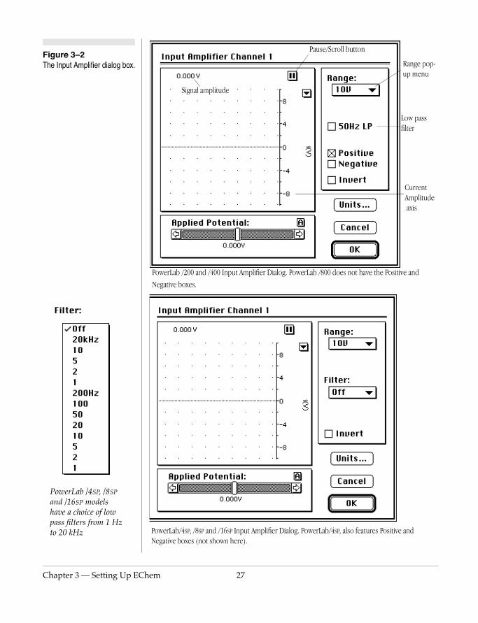
Using the Input Amplifier Dialog Box
The Input Amplifier dialog box (Figure 3–2) allows, among other things, software control of the current recording channel in the PowerLab. For EChem this is channel 1 of the PowerLab. The signal present at that channel’s input is displayed so that you can immediately see the effects of any changes. This allows you to measure the current signal from the potentiostat and use it to check or calibrate this channel to appropriate current units. Once you have changed the settings in the dialog box, click the OK button if you wish to apply the changes to the channel. The Input Amplifier dialog box appears when you click the Input Amplifier… button in the i
Use this pop-up menu to set the range of the i channel to match the output range of the potentiostat
EChem User’s Guide
Channel panel. The dialog box in Figure 3–2 will appear.
Signal Display
The input current signal is displayed so that you can see the effect of changing the settings. Data is not actually being recorded while you do this — as it disappears from the screen it is lost. The incoming signal value is displayed at the top left of the display area. Slowly changing signals will be represented quite accurately, whereas very quickly changing signals will be displayed as a solid dark area showing only the envelope (shape) of the signal formed by the minimum and maximum recorded values.
Chapter 3 — Setting Up EC
Figure 3–2 The Input Amplifier dialog box.
PowerLab /4SP, /8SP and /16SP models have a choice of low pass filters from 1 Hz to 20 kHz
Filter:
Range pop-up menu
Signal amplitude
Pause/Scroll button
Current Amplitude axis
Low pass filter
PowerLab /200 and /400 Input Amplifier Dialog. PowerLab /800 does not have the Positive and
Negative boxes.
hem 27
PowerLab/4SP, /8SP and /16SP Input Amplifier Dialog. PowerLab/4SP, also features Positive and Negative boxes (not shown here).
28
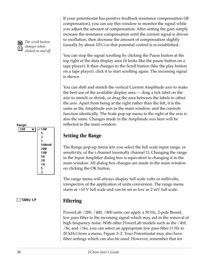
The scroll button changes when clicked on and off
If your potentiostat has positive feedback resistance compensation (iR compensation), you can use this window to monitor the signal while you adjust the amount of compensation. After setting the gain simply increase the resistance compensation until the current signal is driven to oscillation, then decrease the amount of compensation slightly (usually by about 10%) so that potential control is re-established.
You can stop the signal scrolling by clicking the Pause button at the top right of the data display area (it looks like the pause button on a tape player). It then changes to the Scroll button (like the play button on a tape player): click it to start scrolling again. The incoming signal is shown
You can shift and stretch the vertical Current Amplitude axis to make the best use of the available display area — drag a tick label on the axis to stretch or shrink, or drag the area between the labels to offset the axis. Apart from being at the right rather than the left, it is the same as the Amplitude axis in the main window, and the controls function identically. The Scale pop-up menu to the right of the axis is also the same. Changes made in the Amplitude axis here will be reflected in the main window.
Setting the Range
The Range pop-up menu lets you select the full scale input range, or sensitivity, of the i channel (normally channel 1). Changing the range in the Input Amplifier dialog box is equivalent to changing it in the main window. All dialog box changes are made in the main window on clicking the OK button.
EChem User’s Guide
The range menu will always display full scale volts or millivolts, irrespective of the application of units conversion. The range menu starts at +10 V full scale and can be set as low as 2 mV full scale.
Filtering
PowerLab /200, /400, /800 units can apply a 50 Hz, 2-pole Bessel, low pass filter to the incoming signal which may aid in the removal of high frequency noise. With other PowerLab models such as the /4SP, /8s, and /16s, you can select an appropriate low pass filter (1 Hz to 20 kHz) from a menu, Figure 3–2. Your Potentiostat may also have filter settings which can also be used. However, remember that for
Chapter 3 — Setting Up EC
high speed scans, or for work with short period pulses, you will need to keep filtering to a minimum.
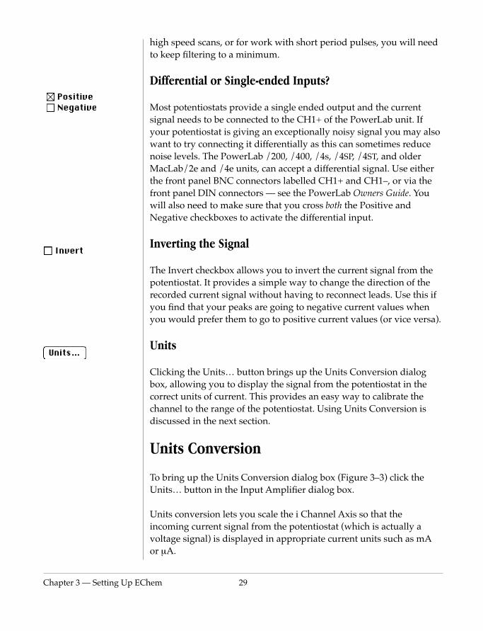
Differential or Single-ended Inputs?
Most potentiostats provide a single ended output and the current signal needs to be connected to the CH1+ of the PowerLab unit. If your potentiostat is giving an exceptionally noisy signal you may also want to try connecting it differentially as this can sometimes reduce noise levels. The PowerLab /200, /400, /4s, /4SP, /4ST, and older MacLab/2e and /4e units, can accept a differential signal. Use either the front panel BNC connectors labelled CH1+ and CH1–, or via the front panel DIN connectors — see the PowerLab Owners Guide. You will also need to make sure that you cross both the Positive and Negative checkboxes to activate the differential input.
Inverting the Signal
The Invert checkbox allows you to invert the current signal from the potentiostat. It provides a simple way to change the direction of the recorded current signal without having to reconnect leads. Use this if you find that your peaks are going to negative current values when you would prefer them to go to positive current values (or vice versa).
Units
Clicking the Units… button brings up the Units Conversion dialog box, allowing you to display the signal from the potentiostat in the correct units of current. This provides an easy way to calibrate the
hem 29
channel to the range of the potentiostat. Using Units Conversion is discussed in the next section.
Units Conversion
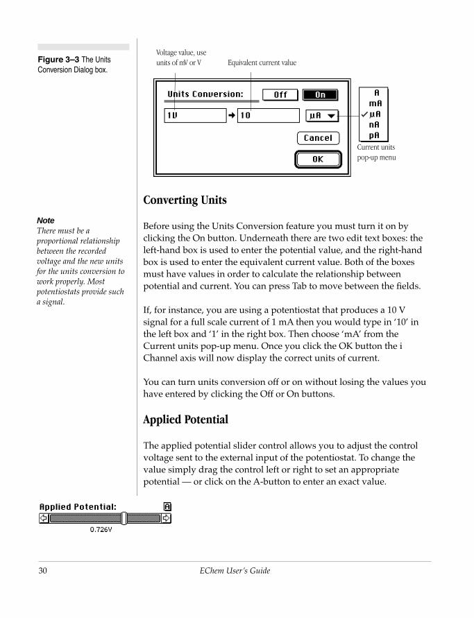
To bring up the Units Conversion dialog box (Figure 3–3) click the Units… button in the Input Amplifier dialog box.
Units conversion lets you scale the i Channel Axis so that the incoming current signal from the potentiostat (which is actually a voltage signal) is displayed in appropriate current units such as mA or µA.
30
Figure 3–3 The Units Conversion Dialog box.
Note There must be a proportional relationship between the recorded voltage and the new units for the units conversion to work properly. Most potentiostats provide such a signal.
Converting Units
Before using the Units Conversion feature you must turn it on by clicking the On button. Underneath there are two edit text boxes: the left-hand box is used to enter the potential value, and the right-hand box is used to enter the equivalent current value. Both of the boxes must have values in order to calculate the relationship between potential and current. You can press Tab to move between the fields.
If, for instance, you are using a potentiostat that produces a 10 V signal for a full scale current of 1 mA then you would type in ‘10’ in the left box and ‘1’ in the right box. Then choose ‘mA’ from the Current units pop-up menu. Once you click the OK button the i Channel axis will now display the correct units of current.
You can turn units conversion off or on without losing the values you have entered by clicking the Off or On buttons.
Current units pop-up menu
Voltage value, use units of mV or V Equivalent current value
EChem User’s Guide
Applied Potential
The applied potential slider control allows you to adjust the control voltage sent to the external input of the potentiostat. To change the value simply drag the control left or right to set an appropriate potential — or click on the A-button to enter an exact value.
Chapter 3 — Setting Up EC
The current range pop-up menu
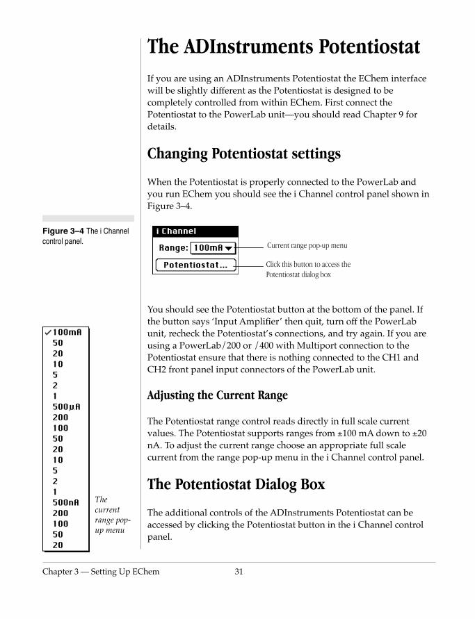
Figure 3–4 The i Channel control panel.
The ADInstruments PotentiostatIf you are using an ADInstruments Potentiostat the EChem interface will be slightly different as the Potentiostat is designed to be completely controlled from within EChem. First connect the Potentiostat to the PowerLab unit—you should read Chapter 9 for details.
Changing Potentiostat settings
When the Potentiostat is properly connected to the PowerLab and you run EChem you should see the i Channel control panel shown in Figure 3–4.
You should see the Potentiostat button at the bottom of the panel. If the button says ‘Input Amplifier’ then quit, turn off the PowerLab unit, recheck the Potentiostat’s connections, and try again. If you are using a PowerLab/200 or /400 with Multiport connection to the Potentiostat ensure that there is nothing connected to the CH1 and CH2 front panel input connectors of the PowerLab unit.
Current range pop-up menu
Click this button to access the Potentiostat dialog box
hem 31
Adjusting the Current Range
The Potentiostat range control reads directly in full scale current values. The Potentiostat supports ranges from ±100 mA down to ±20 nA. To adjust the current range choose an appropriate full scale current from the range pop-up menu in the i Channel control panel.
The Potentiostat Dialog Box
The additional controls of the ADInstruments Potentiostat can be accessed by clicking the Potentiostat button in the i Channel control panel.

32
Figure 3–5 The Potentiostat Input Amplifier dialog box
This dialog (Figure 3–5) allows you to adjust the current range, filtering and cell connection settings. Galvanostat functions are only enabled when using Chart or Scope software, see Chapter 8.
Signal Display
Signal amplitude
Range pop-up menu
Filter pop-up menu
Cell connection modes
Applied potential slider control
Pause Button
Applied potential slider control
EChem User’s Guide
The current signal from the connected cell is shown in the scrolling display area. By using the Dummy or Real modes the effect of an applied potential can be seen prior to actually recording the data. No data is actually recorded when the Potentiostat dialog box is open. When the dialog is closed the signal trace is lost.
You can stop the signal scrolling by clicking the Pause button at the top right of the display area (it looks like the pause button on a tape player). It then changes to the Scroll button (like the play button on a tape player): click it to start scrolling again.
You can shift or stretch the vertical Amplitude axis to make the best use of the available display area. Apart from being at the right rather
Chapter 3 — Setting Up EC
The filter pop-up menu
than the left, it is the same as the amplitude axis in the main EChem window.
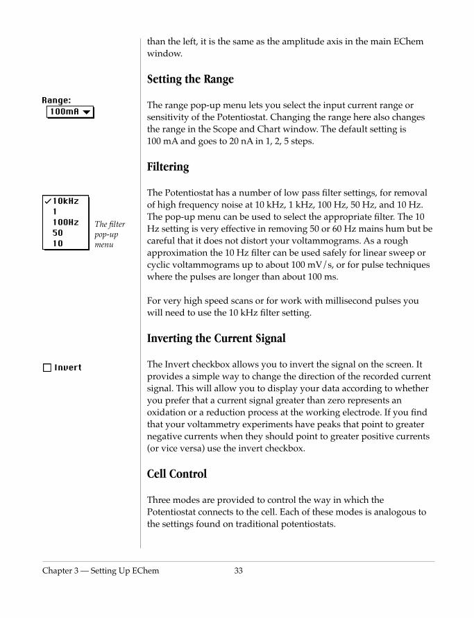
Setting the Range
The range pop-up menu lets you select the input current range or sensitivity of the Potentiostat. Changing the range here also changes the range in the Scope and Chart window. The default setting is 100 mA and goes to 20 nA in 1, 2, 5 steps.
Filtering
The Potentiostat has a number of low pass filter settings, for removal of high frequency noise at 10 kHz, 1 kHz, 100 Hz, 50 Hz, and 10 Hz. The pop-up menu can be used to select the appropriate filter. The 10 Hz setting is very effective in removing 50 or 60 Hz mains hum but be careful that it does not distort your voltammograms. As a rough approximation the 10 Hz filter can be used safely for linear sweep or cyclic voltammograms up to about 100 mV/s, or for pulse techniques where the pulses are longer than about 100 ms.
For very high speed scans or for work with millisecond pulses you will need to use the 10 kHz filter setting.
Inverting the Current Signal
The Invert checkbox allows you to invert the signal on the screen. It provides a simple way to change the direction of the recorded current signal. This will allow you to display your data according to whether
hem 33
you prefer that a current signal greater than zero represents an oxidation or a reduction process at the working electrode. If you find that your voltammetry experiments have peaks that point to greater negative currents when they should point to greater positive currents (or vice versa) use the invert checkbox.
Cell Control
Three modes are provided to control the way in which the Potentiostat connects to the cell. Each of these modes is analogous to the settings found on traditional potentiostats.

34
Standby – the external cell is disconnected and the internal dummy cell is connected to the Potentiostat. When the Potentiostat dialog is closed and the Chart, Scope or EChem start button is clicked the external cell will be connected to enable the experiment. This mode is used if you do not wish to connect to the external cell until the experiment is actually performed. The Applied Potential control is disabled in this mode.
Dummy – the Potentiostat is connected to the internal dummy cell (an internal 100 kΩ resistor network). You can use the Applied Potential slider control to vary the voltage applied to the dummy cell. The Potentiostat will remain connected to the dummy cell even when the Potentiostat dialog is closed and Chart, Scope or EChem is recording. This is useful for testing a method using the dummy cell.
Real – the external cell is connected to the Potentiostat while you are in the Potentiostat dialog. The Applied Potential slider control can be used to adjust the voltage applied to the external cell. When you close the Potentiostat dialog the external cell will be disconnected until the Start button is pressed and Chart, Scope or EChem begins to record an new experiment. This is similar to the Standby mode except it allows you to modify the applied potential before the method is started.
Applied Potential
The applied potential slider control is enabled in either Dummy or Real modes. It allows you to adjust the voltage applied to either the dummy cell or external cell depending on the mode selected. To change the value
EChem User’s Guide
simply drag the control left or right to set an appropriate potential — or click on the A-button to enter an exact value.
Reverse Polarity
Depending on your local convention you may wish to define a ‘more oxidizing potential’ at the working electrode as either a more positive, or as a more negative potential.
If the Reverse Polarity box is crossed then the Potentiostat will produce oxidizing potentials at the working electrode at more

Chapter 3 — Setting Up EC
positive applied potentials. If the box is unchecked then the working electrode becomes more reducing at more positive potentials.
In practice what you might find is that your voltammogram exhibits a peak at (say) 300 mV when it should be at –300 mV. The chances are that the polarity setting is the opposite of what you want. Reverse the polarity and try again.
You can save your preferred polarity convention as the default Start-Up, or as a settings file.
hem 35

36
EChem User’s Guide
EChem
User’s Guide4
C H A P T E R F O U RData Display and Analysis
EChem allows you great flexibility in displaying data. You can change
the lines, patterns, and colors of the display. You can resize the
EChem window, change the size of the channel’s display, or overlay
the voltage and current channel, or invert or interchange the current
and potential axes. You can zoom to see a small section of data in
great detail, or overlay data from any selection of pages in a file.
The whole purpose of recording data, of course, is to find things out
through analysis of the recording. Voltammograms can be measured
using the Cursor, to give absolute coordinates or relative readings
from marker. A background page can be set, so that the
voltammogram on it is subtracted from all others in the file. The
37
inbuilt Data Pad calculates and stores statistics about recorded data,
calculates peak maxima, and areas. The current signal can also be
smoothed, integrated or differentiated according to your
requirements.
This chapter describes the display options available in EChem, from
the basic settings through to Amplitude axis manipulation and the
Zoom window, and also discusses the available analysis options.
38
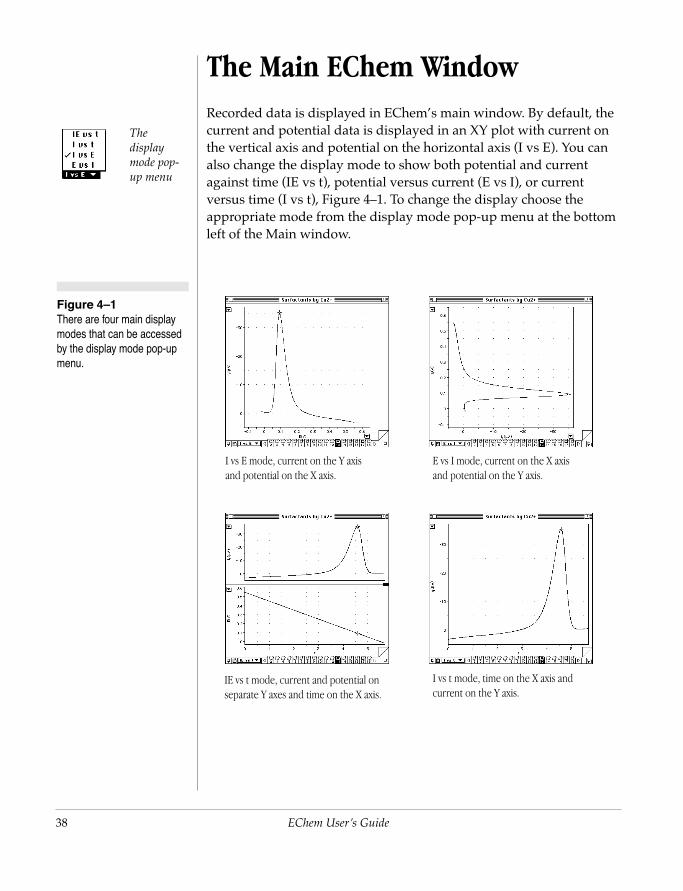
Figure 4–1 There are four main display modes that can be accessed by the display mode pop-up menu.
mode pop-up menu
The Main EChem WindowRecorded data is displayed in EChem’s main window. By default, the current and potential data is displayed in an XY plot with current on the vertical axis and potential on the horizontal axis (I vs E). You can also change the display mode to show both potential and current against time (IE vs t), potential versus current (E vs I), or current versus time (I vs t), Figure 4–1. To change the display choose the appropriate mode from the display mode pop-up menu at the bottom left of the Main window.
I vs E mode, current on the Y axis and potential on the X axis.
E vs I mode, current on the X axis and potential on the Y axis.
The display
EChem User’s Guide
IE vs t mode, current and potential on separate Y axes and time on the X axis.
I vs t mode, time on the X axis and current on the Y axis.

Chapter 4 — Data Display
Figure 4–2 Changing relative heights of the channels and overlaying current and potential data in the IE vs t display mode.
IE vs t Display — Extra Features
When the display is in the IE vs t mode you can vary the relative sizes of the channel display areas Figure 4–2.
Drag the channel separator (the short black bar) up and down, to the desired position — middle picture; or double click the separator to overlay the channels — bottom picture.
Move the pointer over the channel separator. It changes shape:
After you have resized the two channels you can double click the separator to return to equal spacing.
By dragging the separator to the top of the window you can overlay the current and
Position of channel separator in overlay mode. Double click to show separate channels.
and Analysis 39
By dragging the channel separator to the top of the window you can overlay the current and voltage signals — the current axis is on the left, and the potential axis is on the right, Figure 4–2. Both Y axes can be shifted and stretched independently to adjust the graphs as required. The channel separator handle moves to the top right of the window — double-click it to toggle back to separate channel display.
potential traces.

40
Figure 4–3 Using the current axis controls. Similar controls are found on the potential axis.
The AxesThe limits and direction of the current and potential axes can be set from the Scale pop-up menu. The button for which, Figure 4–3, is located on the left-hand side of the current axis (when it is the Y axis) or the lower right hand side of the current axis (when it is the X axis, in E vs I display mode). There is a similar button on the potential axis. The Bipolar and Single Sided options are disabled if Units Conversion is already applied.
The current axis pop-up menu The set scale dialog allows you to
enter exact limits for the axis.
Units Conversion (current axis only) allows you to rescale the output of the potentiostat so
Location of the axis menu button
EChem User’s Guide
it displays the correct units. Computed Functions allow you to transform the data

Chapter 4 — Data Display
Single Sided. Shifts the axis so that zero is located at the bottom (or left) of the display area. This option can be used if you wish to view only current signals larger than zero. Any readings below zero will be off the screen (to see them, select the Bipolar option). If the axis is in bipolar display (below) double clicking it will make it single sided display.
Bipolar. This is the default mode for each channel. It displays zero at the centre of the axis. Double clicking the axis will make it return to bipolar display.
Set Scale. This option allows you to adjust the axis directly to display the range of values you desire. It works whether Units Conversion is on or off. When you choose Set Scale…, the Scale Range dialog box appears (Figure 4–3), allowing you to type in directly the lower and upper limits of the axis to be displayed.
Note that Set Scale is meant for fine-tuning the scale setting rather than for use as a gross magnification tool, and will allow expansion or compression to no more than twice the original range chosen, with neither the upper or lower value being over three times the original limit. First set the range approximately from the Range pop-up menu for the channel, and then set the axis to the precise values required. If you are trying to enlarge very small features you should consider using the Zoom window, or (preferably) recording the data at a higher gain.
Invert Axis. This will reverse the direction of the axis. Useful if you want positive current values to go in the downwards direction (or towards the left when current is on the X axis). The direction of the
and Analysis 41
potential axis can also be reversed so that oxidative potentials can be displayed to the left or right.
Units Conversion… Choosing the Units Conversion item brings up the Units Conversion dialog box (current axis only) which allows you to readjust the conversion factors for the current signal. You have a choice of reassigning conversion factors for all the pages in the file of just for a particular page. See Chapter 3 for more details of Units Conversion.
Computed Functions… Choosing this item is the same as selecting Computed Functions... from the Display menu, and is discussed more
42
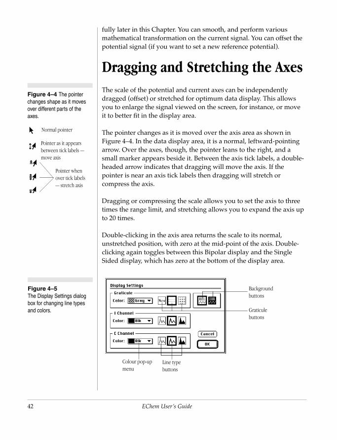
Figure 4–4 The pointer changes shape as it moves over different parts of the axes.
Normal pointer
Pointer as it appears between tick labels —
Figure 4–5 The Display Settings dialog box for changing line types and colors.
fully later in this Chapter. You can smooth, and perform various mathematical transformation on the current signal. You can offset the potential signal (if you want to set a new reference potential).
Dragging and Stretching the AxesThe scale of the potential and current axes can be independently dragged (offset) or stretched for optimum data display. This allows you to enlarge the signal viewed on the screen, for instance, or move it to better fit in the display area.
The pointer changes as it is moved over the axis area as shown in Figure 4–4. In the data display area, it is a normal, leftward-pointing arrow. Over the axes, though, the pointer leans to the right, and a small marker appears beside it. Between the axis tick labels, a double-headed arrow indicates that dragging will move the axis. If the pointer is near an axis tick labels then dragging will stretch or compress the axis.
Dragging or compressing the scale allows you to set the axis to three times the range limit, and stretching allows you to expand the axis up to 20 times.
Double-clicking in the axis area returns the scale to its normal, unstretched position, with zero at the mid-point of the axis. Double-clicking again toggles between this Bipolar display and the Single Sided display, which has zero at the bottom of the display area.
move axis
Pointer when over tick labels — stretch axis
EChem User’s Guide
Background buttons
Line type buttons
Colour pop-up menu
Graticule buttons
Chapter 4 — Data Display
Graticule buttons
Background buttons
Line type buttons
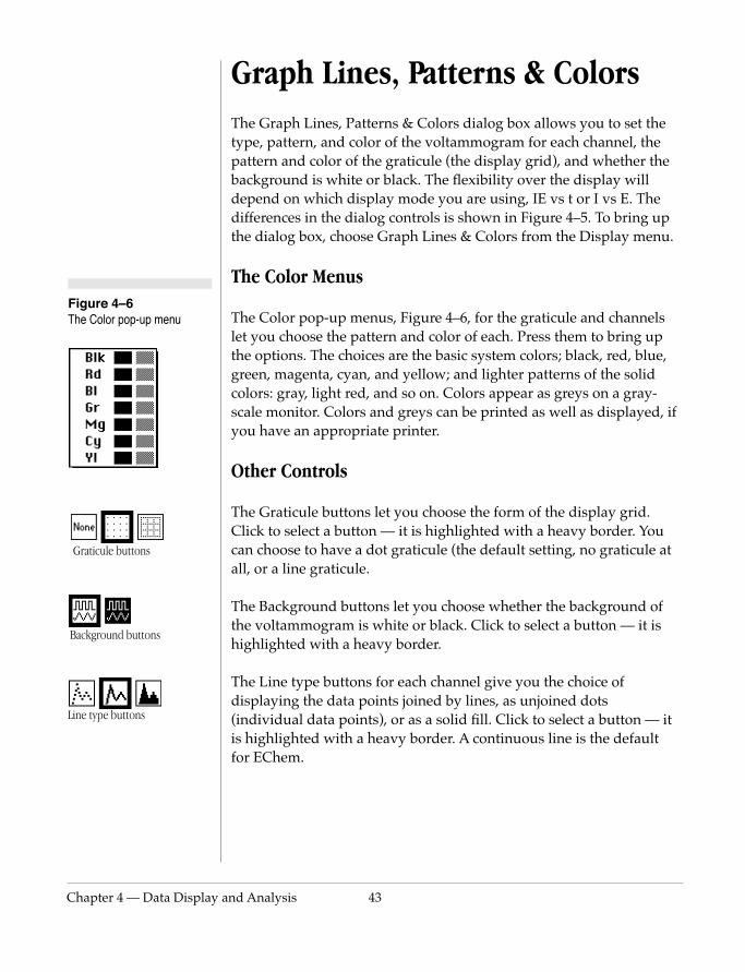
Figure 4–6 The Color pop-up menu
Graph Lines, Patterns & ColorsThe Graph Lines, Patterns & Colors dialog box allows you to set the type, pattern, and color of the voltammogram for each channel, the pattern and color of the graticule (the display grid), and whether the background is white or black. The flexibility over the display will depend on which display mode you are using, IE vs t or I vs E. The differences in the dialog controls is shown in Figure 4–5. To bring up the dialog box, choose Graph Lines & Colors from the Display menu.
The Color Menus
The Color pop-up menus, Figure 4–6, for the graticule and channels let you choose the pattern and color of each. Press them to bring up the options. The choices are the basic system colors; black, red, blue, green, magenta, cyan, and yellow; and lighter patterns of the solid colors: gray, light red, and so on. Colors appear as greys on a gray-scale monitor. Colors and greys can be printed as well as displayed, if you have an appropriate printer.
Other Controls
The Graticule buttons let you choose the form of the display grid. Click to select a button — it is highlighted with a heavy border. You can choose to have a dot graticule (the default setting, no graticule at all, or a line graticule.
The Background buttons let you choose whether the background of
and Analysis 43
the voltammogram is white or black. Click to select a button — it is highlighted with a heavy border.
The Line type buttons for each channel give you the choice of displaying the data points joined by lines, as unjoined dots (individual data points), or as a solid fill. Click to select a button — it is highlighted with a heavy border. A continuous line is the default for EChem.
44
Blank page
Active page
Page Corner controls
Scrolling buttons
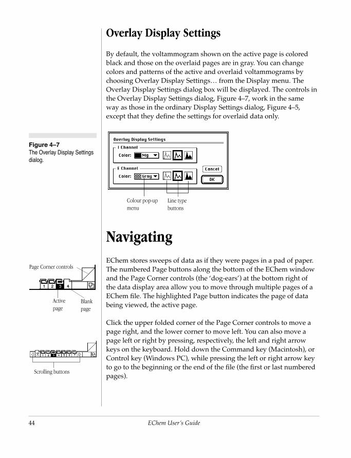
Figure 4–7 The Overlay Display Settings dialog.
Overlay Display Settings
By default, the voltammogram shown on the active page is colored black and those on the overlaid pages are in gray. You can change colors and patterns of the active and overlaid voltammograms by choosing Overlay Display Settings… from the Display menu. The Overlay Display Settings dialog box will be displayed. The controls in the Overlay Display Settings dialog, Figure 4–7, work in the same way as those in the ordinary Display Settings dialog, Figure 4–5, except that they define the settings for overlaid data only.
NavigatingEChem stores sweeps of data as if they were pages in a pad of paper. The numbered Page buttons along the bottom of the EChem window and the Page Corner controls (the ‘dog-ears’) at the bottom right of the data display area allow you to move through multiple pages of a
Colour pop-up menu
Line type buttons
EChem User’s Guide
EChem file. The highlighted Page button indicates the page of data being viewed, the active page.
Click the upper folded corner of the Page Corner controls to move a page right, and the lower corner to move left. You can also move a page left or right by pressing, respectively, the left and right arrow keys on the keyboard. Hold down the Command key (Macintosh), or Control key (Windows PC), while pressing the left or right arrow key to go to the beginning or the end of the file (the first or last numbered pages).
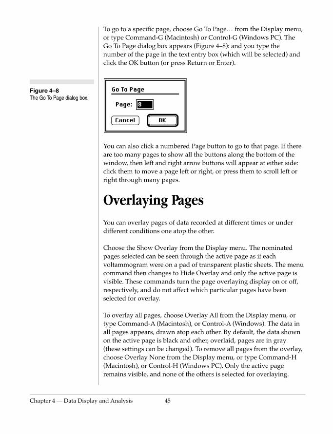
Chapter 4 — Data Display
Figure 4–8 The Go To Page dialog box.
To go to a specific page, choose Go To Page… from the Display menu, or type Command-G (Macintosh) or Control-G (Windows PC). The Go To Page dialog box appears (Figure 4–8): and you type the number of the page in the text entry box (which will be selected) and click the OK button (or press Return or Enter).
You can also click a numbered Page button to go to that page. If there are too many pages to show all the buttons along the bottom of the window, then left and right arrow buttons will appear at either side: click them to move a page left or right, or press them to scroll left or right through many pages.
Overlaying PagesYou can overlay pages of data recorded at different times or under different conditions one atop the other.
Choose the Show Overlay from the Display menu. The nominated pages selected can be seen through the active page as if each voltammogram were on a pad of transparent plastic sheets. The menu command then changes to Hide Overlay and only the active page is
and Analysis 45
visible. These commands turn the page overlaying display on or off, respectively, and do not affect which particular pages have been selected for overlay.
To overlay all pages, choose Overlay All from the Display menu, or type Command-A (Macintosh), or Control-A (Windows). The data in all pages appears, drawn atop each other. By default, the data shown on the active page is black and other, overlaid, pages are in gray (these settings can be changed). To remove all pages from the overlay, choose Overlay None from the Display menu, or type Command-H (Macintosh), or Control-H (Windows PC). Only the active page remains visible, and none of the others is selected for overlaying.
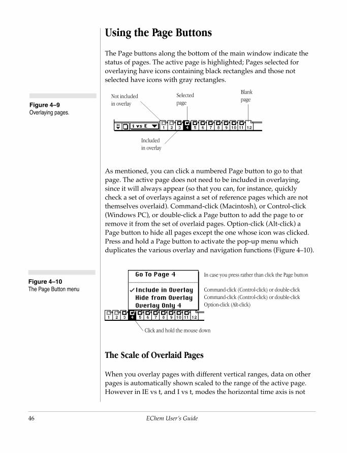
46
Figure 4–10 The Page Button menu
Figure 4–9 Overlaying pages.
Using the Page Buttons
The Page buttons along the bottom of the main window indicate the status of pages. The active page is highlighted; Pages selected for overlaying have icons containing black rectangles and those not selected have icons with gray rectangles.
As mentioned, you can click a numbered Page button to go to that page. The active page does not need to be included in overlaying, since it will always appear (so that you can, for instance, quickly check a set of overlays against a set of reference pages which are not themselves overlaid). Command-click (Macintosh), or Control-click (Windows PC), or double-click a Page button to add the page to or remove it from the set of overlaid pages. Option-click (Alt-click) a Page button to hide all pages except the one whose icon was clicked. Press and hold a Page button to activate the pop-up menu which duplicates the various overlay and navigation functions (Figure 4–10).
Selected page
Included in overlay
Not included in overlay
Blank page
In case you press rather than click the Page button
Command-click (Control-click) or double-click
EChem User’s Guide
The Scale of Overlaid Pages
When you overlay pages with different vertical ranges, data on other pages is automatically shown scaled to the range of the active page. However in IE vs t, and I vs t, modes the horizontal time axis is not
Command-click (Control-click) or double-clickOption-click (Alt-click)
Click and hold the mouse down
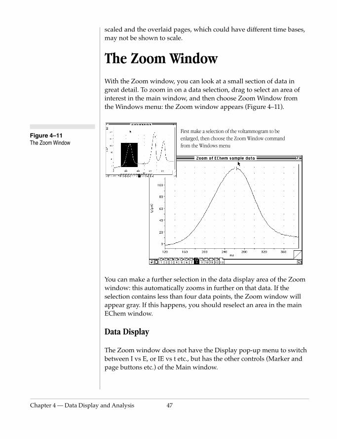
Chapter 4 — Data Display
Figure 4–11 The Zoom Window
scaled and the overlaid pages, which could have different time bases, may not be shown to scale.
The Zoom WindowWith the Zoom window, you can look at a small section of data in great detail. To zoom in on a data selection, drag to select an area of interest in the main window, and then choose Zoom Window from the Windows menu: the Zoom window appears (Figure 4–11).
You can make a further selection in the data display area of the Zoom
First make a selection of the voltammogram to be enlarged, then choose the Zoom Window command from the Windows menu
and Analysis 47
window: this automatically zooms in further on that data. If the selection contains less than four data points, the Zoom window will appear gray. If this happens, you should reselect an area in the main EChem window.
Data Display
The Zoom window does not have the Display pop-up menu to switch between I vs E, or IE vs t etc., but has the other controls (Marker and page buttons etc.) of the Main window.

48
Figure 4–12 The Zoom Window in IE vs t display mode
In IE vs t display mode, if the selection covers only one channel, then only one channel is displayed, and the separator handle is dimmed (see Figure 4-12). If the selection covers two channels, then by default the channels are overlaid, but as in the Main window, double-clicking or dragging the channel separator handle will separate them. Channel overlaying is independent of that in the Main window: you can have the channels separate there and overlaid in the Zoom window, for instance.
Drag the channel separator (the short black bar) up and down, to the desired position or double click the separator to overlay the channels — top picture.
The channel separator in overlay mode. Double click to show separate channels.
EChem User’s Guide
The scale of the vertical axis of each channel can be independently dragged or stretched for optimum data display, just as in the main EChem window.
When moving between pages, the selection area remains the same with regard to the raw data (and will remain in the same relative position in the EChem window).
The Marker from the Main window knows about the Marker in the Zoom window — moving it onto a voltammogram in one window will do the same in the other, double-clicking it will send it to its lair

Chapter 4 — Data Display
— and the Page Comment button will bring up the Page Comment window for the active page.
As you move the pointer across the data display area, the Cursor tracks the displayed data, and the current (i) and potential (E) readings at the tracking point are indicated in the Cursor panel.
Printing the Zoom Window
When the Zoom window is active, then when Print… is chosen from the File menu, the contents of the Zoom window are printed, after the appropriate dialog boxes have been dealt with. The printed page is headed with the window title and the number of the EChem page.
Display and Printer ResolutionEChem allows a flexible data display, so that the display can be rescaled and resized. The controls are not difficult to get used to, especially since the axes are always visible, but they may make the voltammogram look abnormal if you expect it to have the same size and aspect ratio of a standard chart or XY recorder.
The screen display on a monitor is generally about 72 dots per inch, so the apparent resolution is not that good if the display is kept small. The signal might appear jagged and unresolved on a small screen. However, the resolution of the recorded data is independent of the resolution of the display: sampled data is always recorded at 12 bit (0.024%) fidelity at each sensitivity setting. The one important rule is to record your data at the maximum sensitivity (gain) that will keep
and Analysis 49
your voltammogram within the full scale range.
High-resolution printing will show the selected voltammogram accurately. A print-out might not appear as smooth as the pen output of a standard pen recorder if you are using a low resolution dot matrix printer. To get high quality output you should use a laser printer or inkjet printer with a resolution of 300 dpi or greater. Laser printers that use Adobe PostScript® are recommended for maximum quality output.
It is important to check display settings carefully when examining a data, to be sure that what you are looking at is what you think you

50
Figure 4–13 Use of the Pointer and Cursor.
are looking at, especially if the settings on your machine might have been altered. A trace may end up looking very strange if it has been stretched vertically or had an inappropriate baseline subtracted.
Making MeasurementsWhen you have finished recording you can make direct or relative measurements from the voltammogram (or amperomogram).
When the pointer is over the data display area, the Cursor tracks the voltammogram, Figure 4–13. In this case, The Cursor panel shows the current, potential, and time coordinates at the cursor location
The Cursor only gives discrete measurements, jumping from data point to data point (you can see this more clearly in the Zoom window). It cannot provide a reading on the line that is drawn between the individual data points.
Current, potential and time (I, E and t) cursor coordinates
The cursor is attached to the trace but follows the pointer.
The pointer is positioned with the mouse.
EChem User’s Guide
Using the Marker
The Marker can be found in its ‘lair’, a box at the bottom left of the EChem window. It is used to set a particular data point as a zero reference point, so that relative measurements can be made with respect to that point, Figure 4–14. To set the Marker, drag it from its
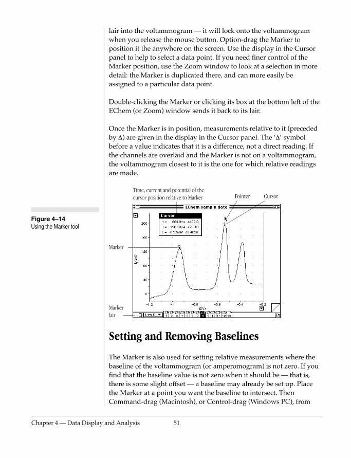
Chapter 4 — Data Display
Figure 4–14 Using the Marker tool
lair into the voltammogram — it will lock onto the voltammogram when you release the mouse button. Option-drag the Marker to position it the anywhere on the screen. Use the display in the Cursor panel to help to select a data point. If you need finer control of the Marker position, use the Zoom window to look at a selection in more detail: the Marker is duplicated there, and can more easily be assigned to a particular data point.
Double-clicking the Marker or clicking its box at the bottom left of the EChem (or Zoom) window sends it back to its lair.
Once the Marker is in position, measurements relative to it (preceded by ∆) are given in the display in the Cursor panel. The ‘∆’ symbol before a value indicates that it is a difference, not a direct reading. If the channels are overlaid and the Marker is not on a voltammogram, the voltammogram closest to it is the one for which relative readings are made.
Time, current and potential of the cursor position relative to Marker
Marker
Pointer Cursor
and Analysis 51
Setting and Removing Baselines
The Marker is also used for setting relative measurements where the baseline of the voltammogram (or amperomogram) is not zero. If you find that the baseline value is not zero when it should be — that is, there is some slight offset — a baseline may already be set up. Place the Marker at a point you want the baseline to intersect. Then Command-drag (Macintosh), or Control-drag (Windows PC), from
Marker lair
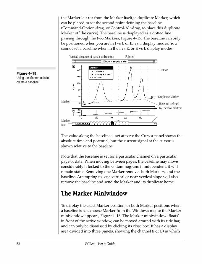
52
Figure 4–15 Using the Marker tools to create a baseline
the Marker lair (or from the Marker itself) a duplicate Marker, which can be placed to set the second point defining the baseline (Command-Option-drag, or Control-Alt-drag, to place this duplicate Marker off the curve). The baseline is displayed as a dotted line passing through the two Markers, Figure 4–15. The baseline can only be positioned when you are in I vs t, or IE vs t, display modes. You cannot set a baseline when in the I vs E, or E vs I, display modes.
The value along the baseline is set at zero: the Cursor panel shows the absolute time and potential, but the current signal at the cursor is shown relative to the baseline.
Note that the baseline is set for a particular channel on a particular page of data. When moving between pages, the baseline may move considerably if locked to the voltammogram; if independent, it will
Marker
Pointer
Duplicate Marker
Baseline defined by the two markers
Cursor
Vertical distance of cursor to baseline
Marker lair
EChem User’s Guide
remain static. Removing one Marker removes both Markers, and the baseline. Attempting to set a vertical or near-vertical slope will also remove the baseline and send the Marker and its duplicate home.
The Marker Miniwindow
To display the exact Marker position, or both Marker positions when a baseline is set, choose Marker from the Windows menu: the Marker miniwindow appears, Figure 4–16. The Marker miniwindow ‘floats’ in front of the active window, can be moved around with its title bar, and can only be dismissed by clicking its close box. It has a display area divided into three panels, showing the channel (i or E) in which
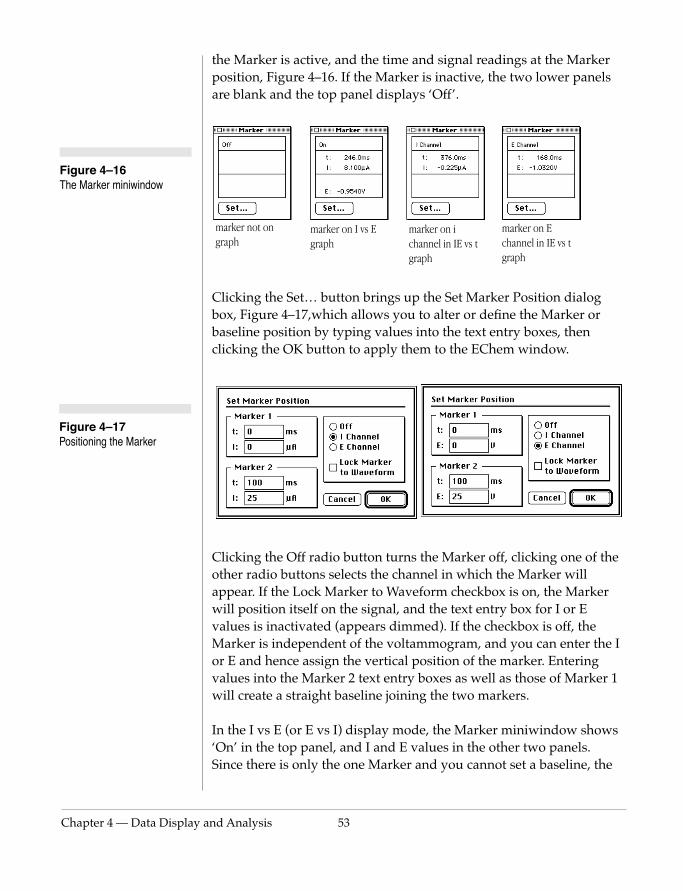
Chapter 4 — Data Display
Figure 4–17 Positioning the Marker
the Marker is active, and the time and signal readings at the Marker position, Figure 4–16. If the Marker is inactive, the two lower panels are blank and the top panel displays ‘Off’.
Clicking the Set… button brings up the Set Marker Position dialog box, Figure 4–17,which allows you to alter or define the Marker or baseline position by typing values into the text entry boxes, then clicking the OK button to apply them to the EChem window.
Clicking the Off radio button turns the Marker off, clicking one of the
marker not on graph
marker on I vs E graph
marker on i channel in IE vs t graph
marker on E channel in IE vs t graph
Figure 4–16 The Marker miniwindow
and Analysis 53
other radio buttons selects the channel in which the Marker will appear. If the Lock Marker to Waveform checkbox is on, the Marker will position itself on the signal, and the text entry box for I or E values is inactivated (appears dimmed). If the checkbox is off, the Marker is independent of the voltammogram, and you can enter the I or E and hence assign the vertical position of the marker. Entering values into the Marker 2 text entry boxes as well as those of Marker 1 will create a straight baseline joining the two markers.
In the I vs E (or E vs I) display mode, the Marker miniwindow shows ‘On’ in the top panel, and I and E values in the other two panels. Since there is only the one Marker and you cannot set a baseline, the
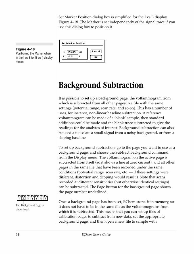
54
The Background page is underlined
Figure 4–18 Positioning the Marker when in the I vs E (or E vs I) display modes
Set Marker Position dialog box is simplified for the I vs E display, Figure 4–18. The Marker is set independently of the signal trace if you use this dialog box to position it.
Background SubtractionIt is possible to set up a background page, the voltammogram from which is subtracted from all other pages in a file with the same settings (potential range, scan rate, and so on). This has a number of uses, for instance, non-linear baseline subtraction. A reference voltammogram can be made of a ‘blank’ sample, then standard additions could be made and the blank trace subtracted to give the readings for the analytes of interest. Background subtraction can also be used a to isolate a small signal from a noisy background, or from a sloping baseline.
To set up background subtraction, go to the page you want to use as a background page, and choose the Subtract Background command from the Display menu. The voltammogram on the active page is subtracted from itself (so it shows a line at zero current), and all other
EChem User’s Guide
pages in the same file that have been recorded under the same conditions (potential range, scan rate, etc. — if these settings were different, distortion and clipping would result.). Note that scans recorded at different sensitivities (but otherwise identical settings) can be subtracted. The Page button for the background page shows the page number underlined.
Once a background page has been set, EChem stores it in memory, so it does not have to be in the same file as the voltammograms from which it is subtracted. This means that you can set up files of calibration pages to subtract from new data, set the appropriate background page, and then open a new file to sample with
Chapter 4 — Data Display
background subtraction. It also means you will not necessarily see the background page button, but the menu commands Subtract Background and Clear Background in the Display menu will be undimmed when a background page is in memory, so this will tell you if such a page has been set.
The Subtract Background command toggles with the Don’t Subtract Background command. Both leave the background page in memory, but will subtract it or not subtract it, respectively, from voltammograms in the open file, so that you can compare voltammograms before and after subtraction.
Choosing Clear Background from the Display menu clears the background page from memory, and restores the raw data.
The Data PadThe Data Pad can store large amounts of data (cursor coordinates, peak maxima and minima etc.) in spreadsheet format — up to 32 columns with 32,000 rows, with each cell having at most 255 characters to a maximum of 2000 characters per row. Its contents can be saved as a text file, or copied to the Clipboard for transfer to other software, or printed directly. To bring up the Data Pad, Figure 4–19, choose Data Pad from the Windows menu.
The Data Pad window is a normal window with a close box, size box, and title bar, and can be moved around the screen or left in the background while the EChem window is active. It can be resized using the size box at its bottom right corner. Click the zoom box to
and Analysis 55
toggle the window between the set size and the full size of the screen.
Information on the current selection or active point is displayed immediately above and beneath the column headings: the readings beneath the column headings are separated from recorded data by a heavy line, and are centered rather than left-justified to help to distinguish them. In EChem, the active point is the last point clicked in the data display area.
As data is added to the Data Pad, new rows of values are created below existing rows in the data area. Use the scroll bars to move down or across through rows and columns. There are two tools that
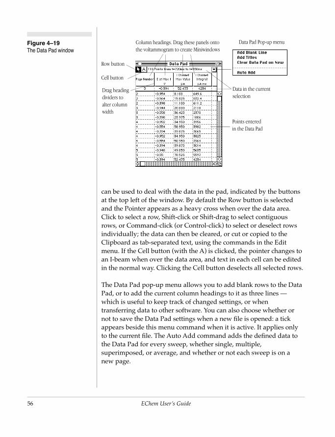
56
Figure 4–19 The Data Pad window
can be used to deal with the data in the pad, indicated by the buttons at the top left of the window. By default the Row button is selected and the Pointer appears as a heavy cross when over the data area. Click to select a row, Shift-click or Shift-drag to select contiguous rows, or Command-click (or Control-click) to select or deselect rows individually; the data can then be cleared, or cut or copied to the Clipboard as tab-separated text, using the commands in the Edit menu. If the Cell button (with the A) is clicked, the pointer changes to an I-beam when over the data area, and text in each cell can be edited in the normal way. Clicking the Cell button deselects all selected rows.
Cell button
Data in the current selection
Data Pad Pop-up menu
Points entered in the Data Pad
Row button
Column headings. Drag these panels onto the voltammogram to create Miniwindows
Drag heading dividers to alter column width
EChem User’s Guide
The Data Pad pop-up menu allows you to add blank rows to the Data Pad, or to add the current column headings to it as three lines — which is useful to keep track of changed settings, or when transferring data to other software. You can also choose whether or not to save the Data Pad settings when a new file is opened: a tick appears beside this menu command when it is active. It applies only to the current file. The Auto Add command adds the defined data to the Data Pad for every sweep, whether single, multiple, superimposed, or average, and whether or not each sweep is on a new page.

Chapter 4 — Data Display
Figure 4–20 Setting up the Data Pad columns
The width of columns can be changed to suit the displayed data and headings. You might want to narrow columns to display more on screen, for example, or have a wide column to the right in which to add comments. Position the pointer on the heavy dividing line between column headings, so that it changes into the resizing pointer, drag until the column is the desired width — a gray line appears, to indicate position — then release the mouse button.
Adding Data to the Data Pad
To add data from a selection in the EChem window to the Data Pad, choose Add to Data Pad from the Windows menu, or type Command-D (Macintosh) or Control-D (Windows PC). If you want to add data on the whole page, the whole page must be selected. Some time-based functions (such as Integral) will only operate when you are in the IE vs t, or I vs t, display modes. If there is no selection, data at the active point is transferred. As a shortcut, you can double-click in the data display area to transfer data at a point (which becomes the active point). This can also be done from the Zoom window; the magnification it provides may prove useful in locating particular features.
The data recorded will depend on the choices made in the Data Pad Column Setup dialog box.
Setting Up the Columns
As previously noted, the data recorded will depend on the choices made in the Data Pad Column Setup dialog box. This dialog box
and Analysis 57
appears on clicking a column heading panel,Figure 4–20, and will have the column number (1 – 32) in its title.
58
To move to the dialog boxes of adjacent columns (and set up many columns quickly), click the arrows by the dialog box title, or press the right or left arrow keys on the keyboard.
The channel that data is taken from is selected in the Channel pop-up menu at the right of the dialog box. Two scrolling lists let you select from the many forms of information that could be recorded, whether derived or direct. The left-hand list gives the general information type, and the right-hand one options available in that set. The selected option is briefly explained in a box beneath the two lists.
Off simply turns the column off: no data is recorded in it.
General Statistics offers calculation of the mean, standard deviation, standard error of the mean, or integration (with respect to time, ∫i.dt) of the selected region of the current signal. The value of the largest or smallest data points in the selection (or the difference between them), the times at which they were recorded, or the number of data points in the selection can also be obtained for the current signal.
Selection Information. If there is a selection, this function will report the start time, end time, or duration.
Cursor. These functions report the time, current and/or potential (t, I and E values) at the active point, if there is one. It does nothing if there is a selection of more than one point.
Slope gives the maximum or minimum slopes (with respect to time, di/dt) found in a selected area of the voltammogram (or amperomogram), the average slope of a selection (the equivalent of
EChem User’s Guide
fitting a straight line through a selection of data points), or the slope of the curve at the active point.
E values can return the magnitude of the potential at the points at which the maximum or minimum current signal (i values) in a selection.
Its various functions make the Data Pad very useful for quickly extracting information about a voltammogram. You can leave the Data Pad, set up to display the required information, as a small visible background window that will be updated as you skip from page to page or as new entries are made.
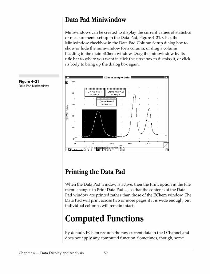
Chapter 4 — Data Display
Figure 4–21 Data Pad Miniwindows
Data Pad Miniwindow
Miniwindows can be created to display the current values of statistics or measurements set up in the Data Pad, Figure 4–21. Click the Miniwindow checkbox in the Data Pad Column Setup dialog box to show or hide the miniwindow for a column, or drag a column heading to the main EChem window. Drag the miniwindow by its title bar to where you want it, click the close box to dismiss it, or click its body to bring up the dialog box again.
Printing the Data Pad
and Analysis 59
When the Data Pad window is active, then the Print option in the File menu changes to Print Data Pad…, so that the contents of the Data Pad window are printed rather than those of the EChem window. The Data Pad will print across two or more pages if it is wide enough, but individual columns will remain intact.
Computed FunctionsBy default, EChem records the raw current data in the I Channel and does not apply any computed function. Sometimes, though, some
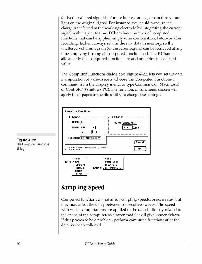
60
Figure 4–22 The Computed Functions dialog
derived or altered signal is of more interest or use, or can throw more light on the original signal. For instance, you could measure the charge transferred at the working electrode by integrating the current signal with respect to time. EChem has a number of computed functions that can be applied singly or in combination, before or after recording. EChem always retains the raw data in memory, so the unaltered voltammogram (or amperomogram) can be retrieved at any time simply by turning all computed functions off. The E Channel allows only one computed function – to add or subtract a constant value.
The Computed Functions dialog box, Figure 4–22, lets you set up data manipulation of various sorts. Choose the Computed Functions… command from the Display menu, or type Command-F (Macintosh) or Control-F (Windows PC). The function, or functions, chosen will apply to all pages in the file until you change the settings.
EChem User’s Guide
Sampling Speed
Computed functions do not affect sampling speeds, or scan rates, but they may affect the delay between consecutive sweeps. The speed with which computations are applied to the data is directly related to the speed of the computer, so slower models will give longer delays. If this proves to be a problem, perform computed functions after the data has been collected.
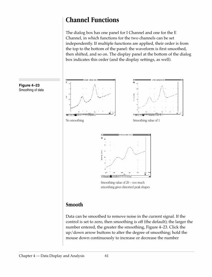
Chapter 4 — Data Display
Figure 4–23 Smoothing of data
Channel Functions
The dialog box has one panel for I Channel and one for the E Channel, in which functions for the two channels can be set independently. If multiple functions are applied, their order is from the top to the bottom of the panel: the waveform is first smoothed, then shifted, and so on. The display panel at the bottom of the dialog box indicates this order (and the display settings, as well).
No smoothing Smoothing value of 1
and Analysis 61
Smooth
Data can be smoothed to remove noise in the current signal. If the control is set to zero, then smoothing is off (the default); the larger the number entered, the greater the smoothing, Figure 4–23. Click the up/down arrow buttons to alter the degree of smoothing; hold the mouse down continuously to increase or decrease the number
Smoothing value of 20 – too much smoothing gives distorted peak shapes

62
rapidly; or type a value in the text box to directly set the degree of smoothing, from 1 to 50. For ‘n’ point smoothing, at each data point ‘p’ the values of the data points in the range p±n are averaged (i.e. a moving point average is taken). At the very start and end of the voltammogram (or amperomogram) there may be insufficient points to complete a full ‘n’ point smoothing and the amount of smoothing will not be as great. Smoothing will affect different waveforms in different ways: voltammograms with sharp peaks cannot be smoothed too much without distortion, but those with broad peaks can be smoothed a lot more.
Math
The Math control lets you add, subtract, multiply or divide the data by a constant amount. By default, the setting is None (no operation is applied) and the text entry box and units control are dimmed. Choose an operation from the Math pop-up menu, Figure 4–22
Add or Subtract. If you choose one of these, the text entry box and units control become usable. You can add or subtract a constant amount from the signal. Type the value in the text box: it can be up to ±30,000, and be set to four decimal places. The units are set by using the up/down arrow buttons. You may want to add or subtract a constant value to the E Channel if you have recorded a voltammogram with a Ag/AgCl electrode but want to change the display so that zero volts corresponds to use of a calomel or standard hydrogen electrode.
Multiply or Divide. If you choose one of these, the text entry box
EChem User’s Guide
becomes usable. (The units control does not, since you are multiplying by a scalar number.) Type the value in the text box: it can be up to ±30,000, and be set to four decimal places, although you cannot enter zero.
Invert. If you choose Invert, the text entry box and units control remain dimmed. Invert changes the sign of the signal, effectively multiplying it by minus one: positive values become negative, and vice-versa. This is usefulness the E channel if you recorded data with one polarity convention (say, more negative potentials mean greater reduction) but then later want to display data with the opposite polarity convention (more negative potentials mean greater reduction).
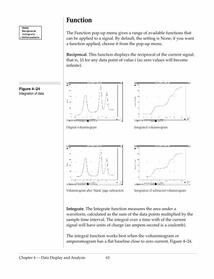
Chapter 4 — Data Display
Figure 4–24 Integration of data
Function
The Function pop-up menu gives a range of available functions that can be applied to a signal. By default, the setting is None; if you want a function applied, choose it from the pop-up menu.
Reciprocal. This function displays the reciprocal of the current signal, that is, 1⁄i for any data point of value i (so zero values will become infinite).
Original voltammogram Integrated voltammogram
and Analysis 63
Integrate. The Integrate function measures the area under a waveform, calculated as the sum of the data points multiplied by the sample time interval. The integral over a time with of the current signal will have units of charge (an ampere.second is a coulomb).
The integral function works best when the voltammogram or amperomogram has a flat baseline close to zero current, Figure 4–24.
Voltammogram after ‘blank’ page subtraction Integration of subtracted voltammogram
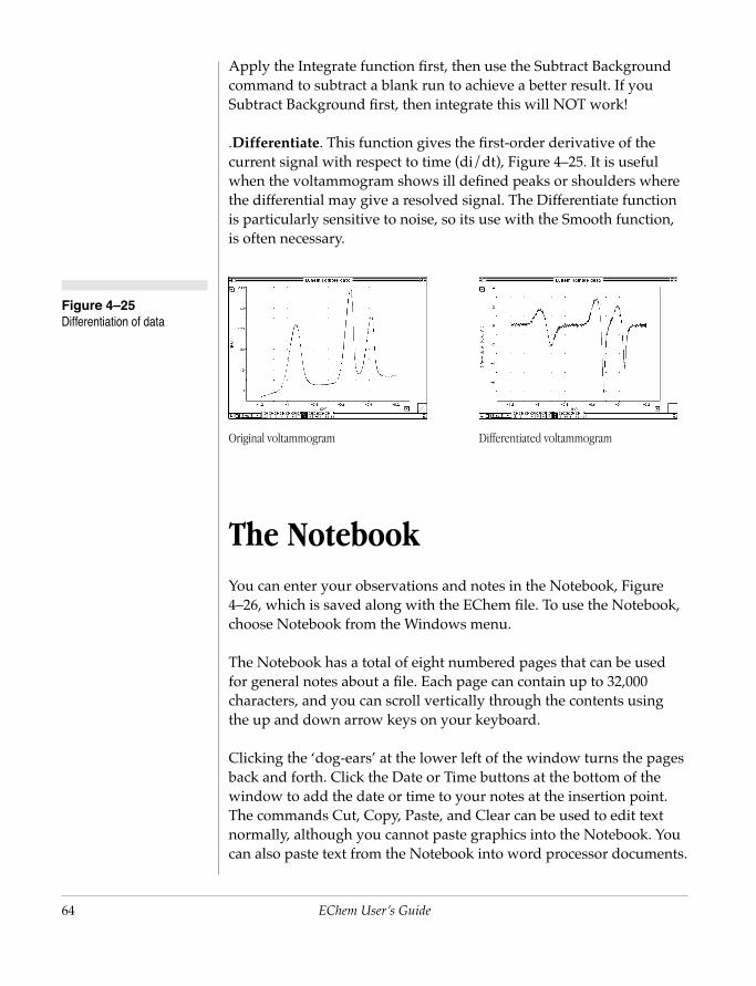
64
Figure 4–25 Differentiation of data
Apply the Integrate function first, then use the Subtract Background command to subtract a blank run to achieve a better result. If you Subtract Background first, then integrate this will NOT work!
.Differentiate. This function gives the first-order derivative of the current signal with respect to time (di/dt), Figure 4–25. It is useful when the voltammogram shows ill defined peaks or shoulders where the differential may give a resolved signal. The Differentiate function is particularly sensitive to noise, so its use with the Smooth function, is often necessary.
The NotebookYou can enter your observations and notes in the Notebook, Figure 4–26, which is saved along with the EChem file. To use the Notebook, choose Notebook from the Windows menu.
Original voltammogram Differentiated voltammogram
EChem User’s Guide
The Notebook has a total of eight numbered pages that can be used for general notes about a file. Each page can contain up to 32,000 characters, and you can scroll vertically through the contents using the up and down arrow keys on your keyboard.
Clicking the ‘dog-ears’ at the lower left of the window turns the pages back and forth. Click the Date or Time buttons at the bottom of the window to add the date or time to your notes at the insertion point. The commands Cut, Copy, Paste, and Clear can be used to edit text normally, although you cannot paste graphics into the Notebook. You can also paste text from the Notebook into word processor documents.
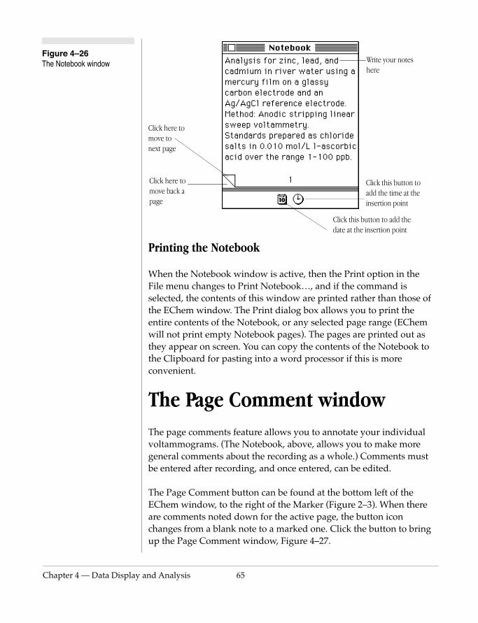
Chapter 4 — Data Display
Figure 4–26 The Notebook window
Printing the Notebook
When the Notebook window is active, then the Print option in the File menu changes to Print Notebook…, and if the command is selected, the contents of this window are printed rather than those of the EChem window. The Print dialog box allows you to print the entire contents of the Notebook, or any selected page range (EChem will not print empty Notebook pages). The pages are printed out as they appear on screen. You can copy the contents of the Notebook to the Clipboard for pasting into a word processor if this is more convenient.
Click here to move to next page
Click here to move back a page
Click this button to add the date at the insertion point
Click this button to add the time at the insertion point
Write your notes here
and Analysis 65
The Page Comment windowThe page comments feature allows you to annotate your individual voltammograms. (The Notebook, above, allows you to make more general comments about the recording as a whole.) Comments must be entered after recording, and once entered, can be edited.
The Page Comment button can be found at the bottom left of the EChem window, to the right of the Marker (Figure 2–3). When there are comments noted down for the active page, the button icon changes from a blank note to a marked one. Click the button to bring up the Page Comment window, Figure 4–27.
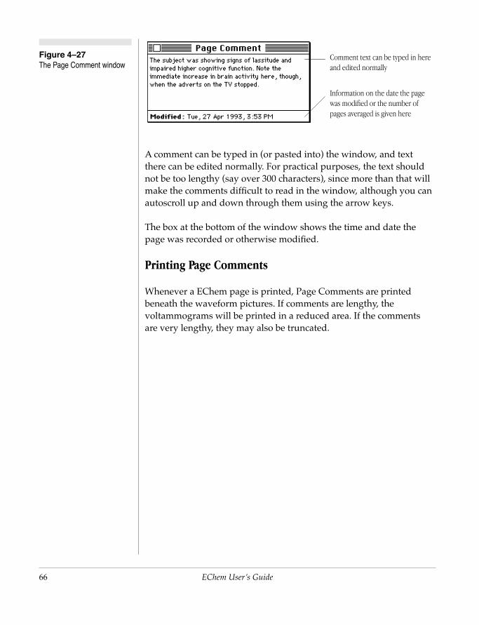
66
Figure 4–27 The Page Comment window
A comment can be typed in (or pasted into) the window, and text there can be edited normally. For practical purposes, the text should not be too lengthy (say over 300 characters), since more than that will make the comments difficult to read in the window, although you can autoscroll up and down through them using the arrow keys.
The box at the bottom of the window shows the time and date the page was recorded or otherwise modified.
Printing Page Comments
Whenever a EChem page is printed, Page Comments are printed beneath the waveform pictures. If comments are lengthy, the voltammograms will be printed in a reduced area. If the comments are very lengthy, they may also be truncated.
Information on the date the page was modified or the number of pages averaged is given here
Comment text can be typed in here and edited normally
EChem User’s Guide

EChem
User’s Guide5
C H A P T E R F I V EWorking With Files
EChem data files can be edited, printed, and saved to disk in various
formats. This chapter describes these operations, and such features as
creating a single file summarising results from many files, and saving
settings to allow easy repetition of an experiment. Other topics
covered include the transfer of data to other programs, such as
spreadsheets and graphing software, and the use of page comments
and the Notebook.
67
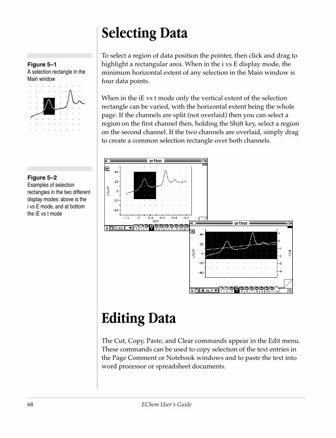
68
Figure 5–2 Examples of selection rectangles in the two different display modes: above is the i vs E mode, and at bottom the iE vs t mode
Selecting DataTo select a region of data position the pointer, then click and drag to highlight a rectangular area. When in the i vs E display mode, the minimum horizontal extent of any selection in the Main window is four data points.
When in the iE vs t mode only the vertical extent of the selection rectangle can be varied, with the horizontal extent being the whole page. If the channels are split (not overlaid) then you can select a region on the first channel then, holding the Shift key, select a region on the second channel. If the two channels are overlaid, simply drag to create a common selection rectangle over both channels.
Figure 5–1 A selection rectangle in the Main window
EChem User’s Guide
Editing DataThe Cut, Copy, Paste, and Clear commands appear in the Edit menu. These commands can be used to copy selection of the text entries in the Page Comment or Notebook windows and to paste the text into word processor or spreadsheet documents.

Chapter 5 — Working With
When the Main window is active, the commands work with whole pages of EChem data rather than selections. Cut removes the active page from the file and places it on the Clipboard. Copy places a copy of the active page on the Clipboard. Paste adds a page already on the Clipboard to the file before the currently selected page. Clear removes the active page from the file. If the Zoom window is active, the active page is still affected rather than the selection that the Zoom window is showing, for most purposes.
All these commands are able to be undone (only a single level of undo is supported). The Undo command, appears in the Edit menu, and changes to reflect your last action. If you have just, for instance, removed a page from the file by choosing Clear from the Edit menu, then the menu command will change to Undo Clear Data. (Should you choose the command again, it becomes Redo Clear Data.)
The editing commands allow you to move pages about and to delete those you do not want. You can move a page between files by placing it on the Clipboard and opening another file (closing the current one, since Scope can only have one file open at a time), then pasting it where it is wanted. Paste inserts the page on the clipboard immediately before the active page.
Transferring DataYou can transfer graphs from EChem to other applications, such as a spreadsheet or drawing program. The Cut and Copy commands place the Main and Zoom windows on the Clipboard as a picture. (The same pictures you would see if the windows were printed, with
Files 69
title, page comments, and so on, but without overlaid pages.) The Clipboard contents can then be pasted into drawing software such as Canvas or CorrelDraw which have extra features to modify the picture for presentation purposes. However the best results are usually obtained by transferring the data itself to a specialist graphing program.
An EChem data file can be saved as an ASCII text file able to be opened by any application that can import text, such as a word processor, spreadsheet, or graphing program such as Igor Pro, Kaleidagraph or Origin (to do this, choose the Save As… menu command from the File menu.)
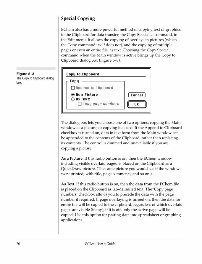
70
Figure 5–3 The Copy to Clipboard dialog box.
Special Copying
EChem also has a more powerful method of copying text or graphics to the Clipboard for data transfer, the Copy Special… command, in the Edit menu. It allows the copying of overlays in pictures (which the Copy command itself does not), and the copying of multiple pages or even an entire file, as text. Choosing the Copy Special… command when the Main window is active brings up the Copy to Clipboard dialog box (Figure 5–3).
The dialog box lets you choose one of two options: copying the Main window as a picture; or copying it as text. If the Append to Clipboard checkbox is turned on, data in text form from the Main window can be appended to the contents of the Clipboard, rather than replacing its contents. The control is dimmed and unavailable if you are copying a picture.
As a Picture. If this radio button is on, then the EChem window, including visible overlaid pages, is placed on the Clipboard as a QuickDraw picture. (The same picture you would see if the window
EChem User’s Guide
were printed, with title, page comments, and so on.)
As Text. If this radio button is on, then the data from the EChem file is placed on the Clipboard as tab-delimited text. The ‘Copy page numbers’ checkbox allows you to precede the data with the page number if required. If page overlaying is turned on, then the data for entire file will be copied to the clipboard, regardless of which overlaid pages are visible (if any); if it is off, only the active page will be copied. Use this option for pasting data into spreadsheet or graphing applications.
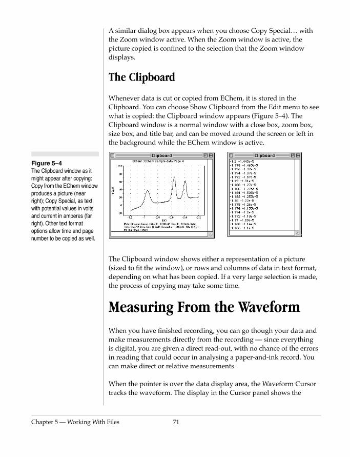
Chapter 5 — Working With
Figure 5–4 The Clipboard window as it might appear after copying: Copy from the EChem window produces a picture (near right); Copy Special, as text, with potential values in volts and current in amperes (far right). Other text format options allow time and page number to be copied as well.
A similar dialog box appears when you choose Copy Special… with the Zoom window active. When the Zoom window is active, the picture copied is confined to the selection that the Zoom window displays.
The Clipboard
Whenever data is cut or copied from EChem, it is stored in the Clipboard. You can choose Show Clipboard from the Edit menu to see what is copied: the Clipboard window appears (Figure 5–4). The Clipboard window is a normal window with a close box, zoom box, size box, and title bar, and can be moved around the screen or left in the background while the EChem window is active.
The Clipboard window shows either a representation of a picture (sized to fit the window), or rows and columns of data in text format, depending on what has been copied. If a very large selection is made, the process of copying may take some time.
Files 71
Measuring From the WaveformWhen you have finished recording, you can go though your data and make measurements directly from the recording — since everything is digital, you are given a direct read-out, with no chance of the errors in reading that could occur in analysing a paper-and-ink record. You can make direct or relative measurements.
When the pointer is over the data display area, the Waveform Cursor tracks the waveform. The display in the Cursor panel shows the
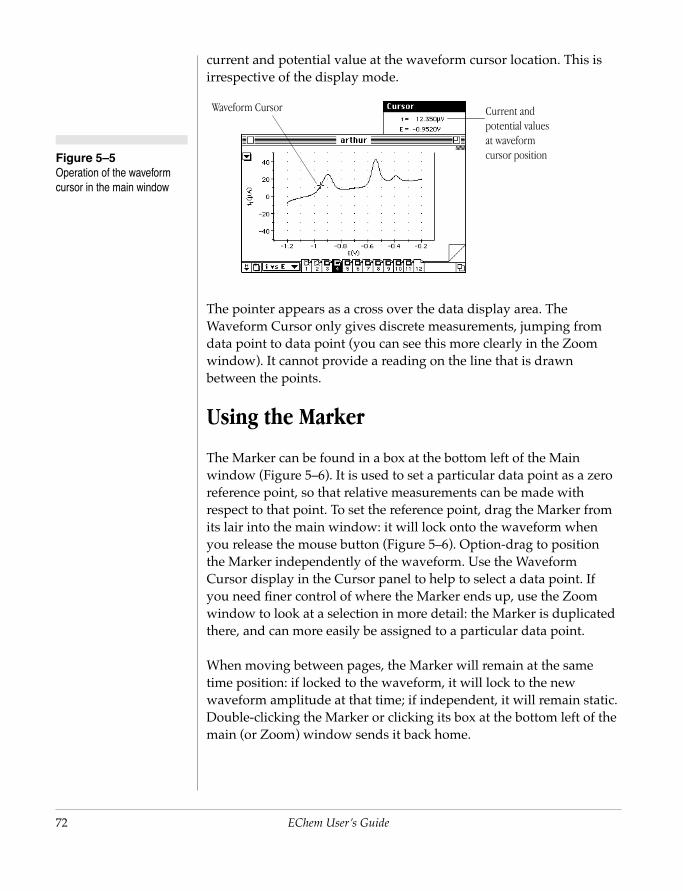
72
Figure 5–5 Operation of the waveform cursor in the main window
current and potential value at the waveform cursor location. This is irrespective of the display mode.
The pointer appears as a cross over the data display area. The Waveform Cursor only gives discrete measurements, jumping from data point to data point (you can see this more clearly in the Zoom window). It cannot provide a reading on the line that is drawn between the points.
Using the Marker
The Marker can be found in a box at the bottom left of the Main window (Figure 5–6). It is used to set a particular data point as a zero reference point, so that relative measurements can be made with respect to that point. To set the reference point, drag the Marker from its lair into the main window: it will lock onto the waveform when you release the mouse button (Figure 5–6). Option-drag to position the Marker independently of the waveform. Use the Waveform
Current and potential values at waveform cursor position
Waveform Cursor
EChem User’s Guide
Cursor display in the Cursor panel to help to select a data point. If you need finer control of where the Marker ends up, use the Zoom window to look at a selection in more detail: the Marker is duplicated there, and can more easily be assigned to a particular data point.
When moving between pages, the Marker will remain at the same time position: if locked to the waveform, it will lock to the new waveform amplitude at that time; if independent, it will remain static. Double-clicking the Marker or clicking its box at the bottom left of the main (or Zoom) window sends it back home.

Chapter 5 — Working With
Figure 5–6 The operation of the marker and waveform cursor in the main window.
Once the Marker is in position, current measurements relative to it (preceded by ∆) are given in the Waveform Cursor display. The potential at the Waveform Cursor position is absolute. The ‘∆’ symbol before the current value indicates that it is a difference, not a direct reading.
Setting and Removing Baselines
In iE vs t display mode the Marker can also used for setting relative amplitude measurements where the baseline of a channel is not zero. Once you have recorded a waveform, you may find that the baseline value is not at zero potential (or set units) when it should be –that is, there is some slight offset. You may want to measure features of a waveform relative to a series of other features. In either case, a baseline should be set up for the channel of interest. To do this, place the Marker at a point you want the baseline to intersect. Then Command-drag from the Marker lair or the Marker itself: this creates
Amplitude of current at the Waveform Cursor position relative to Marker
Marker
Markers lair
Files 73
a duplicate Marker, which can be placed in the same channel to set the second point the baseline intersects (Command-Option-drag to place this duplicate independently of the waveform). The baseline is displayed as a dotted line passing through the two Markers.
The value along the baseline is set at zero: the Waveform Cursor display in the Cursor panel shows the absolute potential, and the amplitude of the current relative to the baseline (Figure 5–7).
Note that the baseline is set for a particular page of data. When moving between pages, the baseline may move considerably if locked to the waveform; if independent, it will remain static. Removing one Marker removes both Markers, and the baseline.
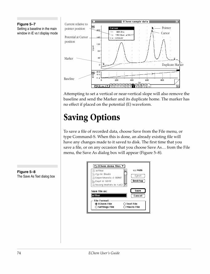
74
Figure 5–8 The Save As Text dialog box
Figure 5–7 Setting a baseline in the main window in iE vs t display mode
Attempting to set a vertical or near-vertical slope will also remove the baseline and send the Marker and its duplicate home. The marker has no effect if placed on the potential (E) waveform.
Saving OptionsTo save a file of recorded data, choose Save from the File menu, or type Command-S. When this is done, an already existing file will have any changes made to it saved to disk. The first time that you save a file, or on any occasion that you choose Save As… from the File menu, the Save As dialog box will appear (Figure 5–8).
Current relative to pointer position
Potential at Cursor position
Marker
Pointer
Duplicate Marker
Baseline
Cursor
EChem User’s Guide

Chapter 5 — Working With
The dialog box allows you to navigate through the file system of the Macintosh to choose where your file will be saved. (You should be familiar with this process; if not, see your Macintosh User’s Guide for directions.) Once you have typed in a name for the file, you can select a file format by clicking one of the radio buttons in the lower portion of the dialog box, and then save the file by clicking the Save button. You can save multiple copies of a file in any format or formats, provided that the copies have different names or are in different folders.
Data File
In this format, which is the default, both data and settings (including macros) are saved. The file chronicles the entire recording, and is the usual way you would want to save data. EChem can open only one file at a time. Opening a data file will close an already opened file.
Settings File
This format does not save any recorded data, only the settings. Settings include the technique, current range, and those that affect the way the data looks, such as the window size, display settings, and menu configuration. Macros are also stored as settings. Using settings files, you can build up a library of settings for many different experiments, to enable quick and easy preparation for recording.
Settings files have a different icon from other EChem files. Double-clicking on a settings file icon from the Finder will automatically load the settings from that file into a new untitled EChem file. Opening a
Files 75
settings file using the Open directory dialog box with the Load Settings checkbox selected loads the settings into the current file.
Text File
This format saves data as a standard text file able to be opened by any application that can import text, such as a word processor, spread-sheet, or statistics package. Each data point is stored as a row of numbers comprising the page number, time (t, in seconds), potential (E, in volts) and current (I, in amperes) values, in that order, separated by tabs.
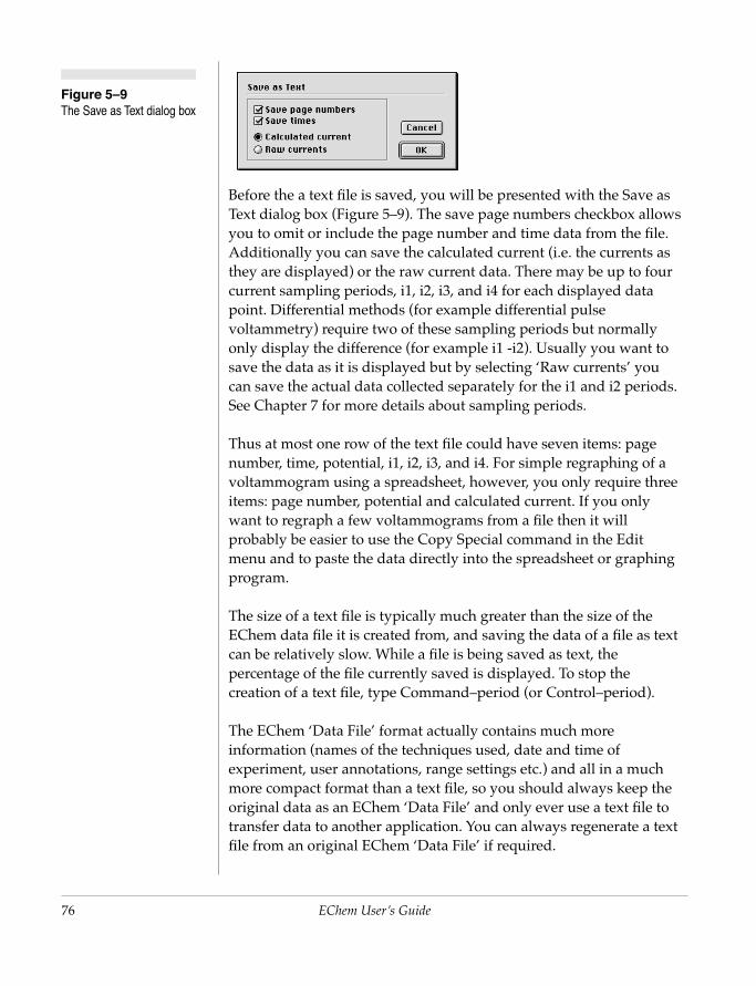
76
Figure 5–9 The Save as Text dialog box
Before the a text file is saved, you will be presented with the Save as Text dialog box (Figure 5–9). The save page numbers checkbox allows you to omit or include the page number and time data from the file. Additionally you can save the calculated current (i.e. the currents as they are displayed) or the raw current data. There may be up to four current sampling periods, i1, i2, i3, and i4 for each displayed data point. Differential methods (for example differential pulse voltammetry) require two of these sampling periods but normally only display the difference (for example i1 -i2). Usually you want to save the data as it is displayed but by selecting ‘Raw currents’ you can save the actual data collected separately for the i1 and i2 periods. See Chapter 7 for more details about sampling periods.
Thus at most one row of the text file could have seven items: page number, time, potential, i1, i2, i3, and i4. For simple regraphing of a voltammogram using a spreadsheet, however, you only require three items: page number, potential and calculated current. If you only want to regraph a few voltammograms from a file then it will probably be easier to use the Copy Special command in the Edit menu and to paste the data directly into the spreadsheet or graphing program.
The size of a text file is typically much greater than the size of the
EChem User’s Guide
EChem data file it is created from, and saving the data of a file as text can be relatively slow. While a file is being saved as text, the percentage of the file currently saved is displayed. To stop the creation of a text file, type Command–period (or Control–period).
The EChem ‘Data File’ format actually contains much more information (names of the techniques used, date and time of experiment, user annotations, range settings etc.) and all in a much more compact format than a text file, so you should always keep the original data as an EChem ‘Data File’ and only ever use a text file to transfer data to another application. You can always regenerate a text file from an original EChem ‘Data File’ if required.
Chapter 5 — Working With
Macro File
This format saves any macros currently in memory as a separate file, which can be opened by EChem as required. It is useful to save particular groups of macros together.
Macro files have a different icon from other EChem files. Double-clicking on a macro file icon from the Finder will automatically load the macros from that file into a new untitled EChem file. Opening a macro file using the Open directory dialog box (whether or not the Load Settings checkbox is on) loads the macro into the current file.
Appending FilesThis feature allows any EChem data file to be appended to the end of an already open file in order to produce a single file with the desired contents. By combining this feature with EChem’s ability to cut and paste pages of data in a file or between files, summary files can be created using only those segments of recordings that have significance. Appending a file is an option provided in the Open directory dialog box: choose Open… from the File menu. (If you have made changes to your file since last you saved, you will be asked if you want to save them.) The Open directory dialog box appears (Figure 5–10) and by default only EChem files are shown in the scrolling list. You can navigate through your hard disk using the Macintosh hierarchical file system to find the file you want.
Click the Append to Current File checkbox to turn it on. Note that the Load Settings checkbox becomes dimmed and unusable, since the
Files 77
appended file takes on the settings currently in memory. This may result in some scale changes, but the raw data will not be altered. Select the EChem file you wish to append to the currently open file, and click the Open button to perform the operation. The pages will be added on to the end of the current file.
Text FilesEChem can open text files, or append them to already open files. To do this, choose Open… from the File menu. The Open directory dialog box appears (Figure 5–10) — click the Text Files radio button
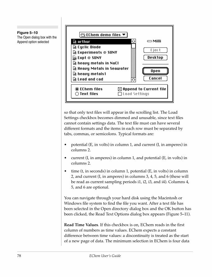
78
Figure 5–10 The Open dialog box with the Append option selected
so that only text files will appear in the scrolling list. The Load Settings checkbox becomes dimmed and unusable, since text files cannot contain settings data. The text file must can have several different formats and the items in each row must be separated by tabs, commas, or semicolons. Typical formats are:
• potential (E, in volts) in column 1, and current (I, in amperes) in columns 2.
• current (I, in amperes) in column 1, and potential (E, in volts) in columns 2.
• time (t, in seconds) in column 1, potential (E, in volts) in column 2, and current (I, in amperes) in columns 3, 4, 5, and 6 (these will
EChem User’s Guide
be read as current sampling periods i1, i2, i3, and i4). Columns 4, 5, and 6 are optional.
You can navigate through your hard disk using the Macintosh or Windows file system to find the file you want. After a text file has been selected in the Open directory dialog box and the OK button has been clicked, the Read Text Options dialog box appears (Figure 5–11).
Read Time Values. If this checkbox is on, EChem reads in the first column of numbers as time values. EChem expects a constant difference between time values: a discontinuity is treated as the start of a new page of data. The minimum selection in EChem is four data

Chapter 5 — Working With
Figure 5–11 The Read Text Options dialog box
points: thus any times read in must have at least three consecutive intervals the same to create a new EChem page of data. If times are not read in, then the EChem Time axis will have no units.
The Time Units radio buttons allow you to specify the time units of the time values.
EChem first scans the file to see if it is in order. If there is a problem, such as erratic time values or text where it expected numbers, it alerts you and does not load the file. It also allows you to
Pasting in Text
Copied text from data files (such as Scope software) of other software can be pasted into EChem directly. The text copied to the clipboard must be in a correct format.
Files 79
PrintingPrinting an EChem file or parts of it will give you a hard copy of your data for use in reports and presentations. There are two menu commands in the File menu concerned with printing: Page Setup… and the basic Print… command (with a keyboard equivalent of Command-P, or Control-P), which may change depending on what can be printed at the time.
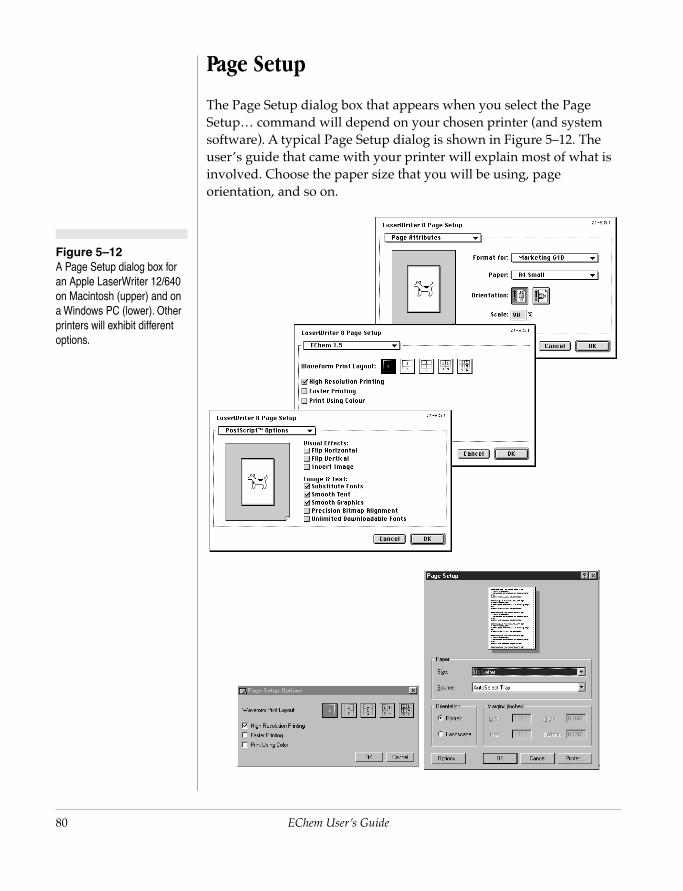
80
Figure 5–12 A Page Setup dialog box for an Apple LaserWriter 12/640 on Macintosh (upper) and on a Windows PC (lower). Other printers will exhibit different options.
Page Setup
The Page Setup dialog box that appears when you select the Page Setup… command will depend on your chosen printer (and system software). A typical Page Setup dialog is shown in Figure 5–12. The user’s guide that came with your printer will explain most of what is involved. Choose the paper size that you will be using, page orientation, and so on.
EChem User’s Guide
Chapter 5 — Working With
NoteFor the best possible printing, ensure that you are using the latest version printer driver for your particular printer. Many manufacturers allow you to download the latest printer drivers from their web sites.
Waveform Print Layout
Click the appropriate Waveform Print Layout buttons to print one, two, three, four, or six EChem pages per printed sheet of paper. By default, the leftmost button is selected, and one EChem page appears on a printed sheet. The page range specified when printing refers to EChem pages, not pieces of paper produced: printing six pages would, if the rightmost Waveform Print Layout button were selected, produce one printed sheet with the six data pages on it.
On a Macintosh this feature will work in conjunction with the Layout option in the LaserWriter 8 Print dialog box, which gives you the choice of one, two, or four, eight or sixteen pages per sheet of paper, so that you could print up to 48 EChem pages per sheet — but this would results in tiny graphs!
High-Resolution Printing
Some printers support several modes of resolution. Checking this option allows you to print the EChem or Zoom windows at the maximum resolution of the printer. For example, if you are using a 600 dpi laser printer, EChem will print with a resolution of 600 dots per inch. This will result in output of the best possible quality, but, since every data point and connecting line is drawn at full resolution, printing may be slow.
Without high-resolution printing, the accuracy of positioning items (data points, axis tick marks and labels, etc.) is not as accurate on the printed page. This may still be adequate for drafts and overviews,
Files 81
and will result in quicker printing.
Faster Printing
If Faster Printing is not selected, EChem passes the recorded data to the printer driver, which generates a set of instructions which are passed to the printer. If there are many data points in the file, the printer driver software has to work harder at converting the data points into the printer instructions, which will take more time.
When Faster Printing is selected, EChem attempts to speed up printing by creating a bitmapped image of the data to be printed.
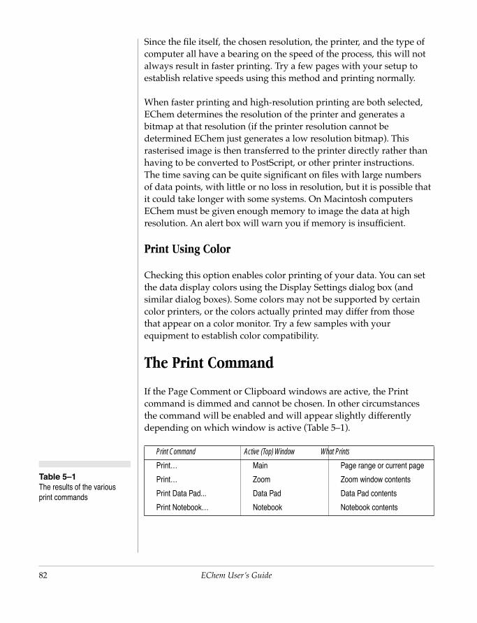
82
Table 5–1 The results of the various print commands
Since the file itself, the chosen resolution, the printer, and the type of computer all have a bearing on the speed of the process, this will not always result in faster printing. Try a few pages with your setup to establish relative speeds using this method and printing normally.
When faster printing and high-resolution printing are both selected, EChem determines the resolution of the printer and generates a bitmap at that resolution (if the printer resolution cannot be determined EChem just generates a low resolution bitmap). This rasterised image is then transferred to the printer directly rather than having to be converted to PostScript, or other printer instructions. The time saving can be quite significant on files with large numbers of data points, with little or no loss in resolution, but it is possible that it could take longer with some systems. On Macintosh computers EChem must be given enough memory to image the data at high resolution. An alert box will warn you if memory is insufficient.
Print Using Color
Checking this option enables color printing of your data. You can set the data display colors using the Display Settings dialog box (and similar dialog boxes). Some colors may not be supported by certain color printers, or the colors actually printed may differ from those that appear on a color monitor. Try a few samples with your equipment to establish color compatibility.
The Print Command
If the Page Comment or Clipboard windows are active, the Print
EChem User’s Guide
command is dimmed and cannot be chosen. In other circumstances the command will be enabled and will appear slightly differently depending on which window is active (Table 5–1).
Print Command Active (Top) Window What Prints
Print… Main Page range or current page
Print… Zoom Zoom window contents
Print Data Pad... Data Pad Data Pad contents
Print Notebook… Notebook Notebook contents
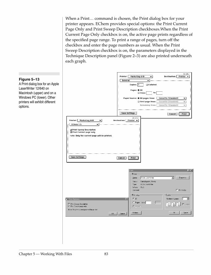
Chapter 5 — Working With
Figure 5–13 A Print dialog box for an Apple LaserWriter 12/640 on Macintosh (upper) and on a Windows PC (lower). Other printers will exhibit different options.
When a Print… command is chosen, the Print dialog box for your printer appears. EChem provides special options: the Print Current Page Only and Print Sweep Description checkboxes.When the Print Current Page Only checkbox is on, the active page prints regardless of the specified page range. To print a range of pages, turn off the checkbox and enter the page numbers as usual. When the Print Sweep Description checkbox is on, the parameters displayed in the Technique Description panel (Figure 2–3) are also printed underneath each graph.
Files 83
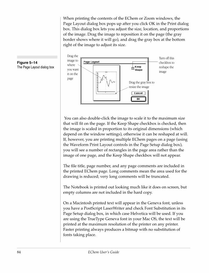
84
Figure 5–14 The Page Layout dialog box
When printing the contents of the EChem or Zoom windows, the Page Layout dialog box pops up after you click OK in the Print dialog box. This dialog box lets you adjust the size, location, and proportions of the image. Drag the image to reposition it on the page (the gray border shows where it will go), and drag the gray box at the bottom right of the image to adjust its size.
You can also double-click the image to scale it to the maximum size that will fit on the page. If the Keep Shape checkbox is checked, then the image is scaled in proportion to its original dimensions (which depend on the window settings), otherwise it can be reshaped at will. If, however, you are printing multiple EChem pages on a page (using the Waveform Print Layout controls in the Page Setup dialog box), you will see a number of rectangles in the page area rather than the image of one page, and the Keep Shape checkbox will not appear.
The file title, page number, and any page comments are included in the printed EChem page. Long comments mean the area used for the
Drag the image to where you want it on the page
Drag the gray box to resize the image
Turn off this checkbox to reshape the image
EChem User’s Guide
drawing is reduced; very long comments will be truncated.
The Notebook is printed out looking much like it does on screen, but empty columns are not included in the hard copy.
On a Macintosh printed text will appear in the Geneva font, unless you have a PostScript LaserWriter and check Font Substitution in its Page Setup dialog box, in which case Helvetica will be used. If you are using the TrueType Geneva font in your Mac OS, the text will be printed at the maximum resolution of the printer on any printer. Faster printing always produces a bitmap with no substitution of fonts taking place.

Chapter 5 — Working With
On a Windows PC a default font will be used.
While the file is printing (or being spooled, if you are printing in the background) a small dialog box appears. Click its Cancel button to stop printing (or type Command-period, or Control-Period, or press the Return, Enter, or Esc keys).
Files 85

86
EChem User’s Guide
EChem
User’s Guide6
C H A P T E R S I XCustomizing & Automating EChem
You can to customise and to automate functions within EChem,
greatly increasing its convenience and ease of use. It can be simplified
or modified by:
• locking or hiding menus or commands with the Menu Editor
• altering controls, menus, and menu commands, and moving
control panels then store your changes as a Settings File or as
the Default Startup.
• storing techniques with preconfigured parameters (initial and
final potentials, scan rates, pulse heights etc.) as Settings Files.
87
• automate complex tasks by creating multi-step Macro
commands which can be stored as new commends in new or
existing menus.
This chapter looks in detail at these various ways of altering EChem
to suit your experimental requirements.
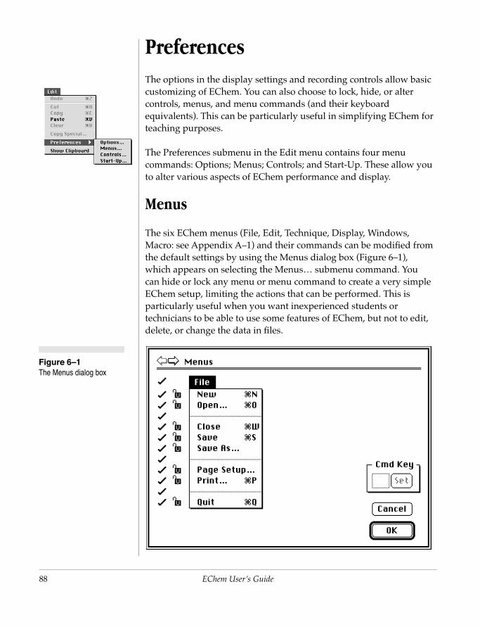
88
Figure 6–1 The Menus dialog box
PreferencesThe options in the display settings and recording controls allow basic customizing of EChem. You can also choose to lock, hide, or alter controls, menus, and menu commands (and their keyboard equivalents). This can be particularly useful in simplifying EChem for teaching purposes.
The Preferences submenu in the Edit menu contains four menu commands: Options; Menus; Controls; and Start-Up. These allow you to alter various aspects of EChem performance and display.
Menus
The six EChem menus (File, Edit, Technique, Display, Windows, Macro: see Appendix A–1) and their commands can be modified from the default settings by using the Menus dialog box (Figure 6–1), which appears on selecting the Menus… submenu command. You can hide or lock any menu or menu command to create a very simple EChem setup, limiting the actions that can be performed. This is particularly useful when you want inexperienced students or technicians to be able to use some features of EChem, but not to edit, delete, or change the data in files.
EChem User’s Guide
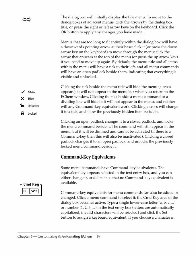
Chapter 6 — Customizing
The dialog box will initially display the File menu. To move to the dialog boxes of adjacent menus, click the arrows by the dialog box title, or press the right or left arrow keys on the keyboard. Click the OK button to apply any changes you have made.
Menus that are too long to fit entirely within the dialog box will have a downwards pointing arrow at their base: click it (or press the down arrow key on the keyboard) to move through the menu; click the arrow that appears at the top of the menu (or press the up arrow key) if you need to move up again. By default, the menu title and all items within the menu will have a tick to their left, and all menu commands will have an open padlock beside them, indicating that everything is visible and unlocked.
Clicking the tick beside the menu title will hide the menu (a cross appears): it will not appear in the menu bar when you return to the EChem window. Clicking the tick beside a menu command or a dividing line will hide it: it will not appear in the menu, and neither will any Command-key equivalent work. Clicking a cross will change it to a tick, and show the previously hidden item beside it.
Clicking an open padlock changes it to a closed padlock, and locks the menu command beside it. The command will still appear in the menu, but it will be dimmed and cannot be activated (if there is a Command-key then this will also be inactivated). Clicking a closed padlock changes it to an open padlock, and unlocks the previously locked menu command beside it.
Command-Key Equivalents
& Automating EChem 89
Some menu commands have Command-key equivalents. The equivalent key appears selected in the text entry box, and you can either change it, or delete it so that no Command-key equivalent is available.
Command-key equivalents for menu commands can also be added or changed. Click a menu command to select it: the Cmd Key area of the dialog box becomes active. Type a single lower-case letter (a, b, c, ...) or number (1, 2, 3, ...) in the text entry box (letters are automatically capitalized; invalid characters will be rejected) and click the Set button to assign a keyboard equivalent. If you choose a character in
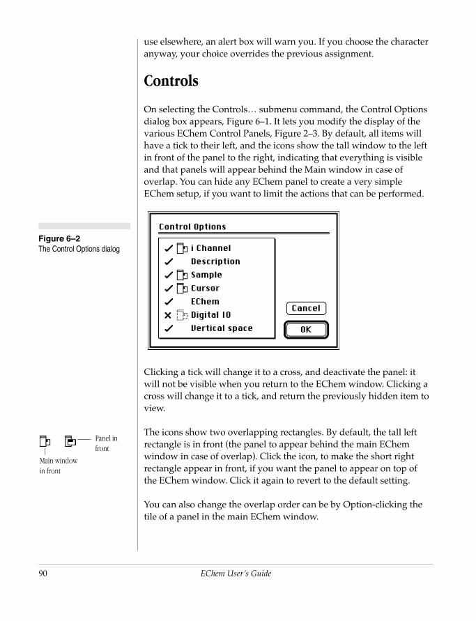
90
Figure 6–2 The Control Options dialog
Main window in front
Panel in front
use elsewhere, an alert box will warn you. If you choose the character anyway, your choice overrides the previous assignment.
Controls
On selecting the Controls… submenu command, the Control Options dialog box appears, Figure 6–1. It lets you modify the display of the various EChem Control Panels, Figure 2–3. By default, all items will have a tick to their left, and the icons show the tall window to the left in front of the panel to the right, indicating that everything is visible and that panels will appear behind the Main window in case of overlap. You can hide any EChem panel to create a very simple EChem setup, if you want to limit the actions that can be performed.
Clicking a tick will change it to a cross, and deactivate the panel: it will not be visible when you return to the EChem window. Clicking a cross will change it to a tick, and return the previously hidden item to
EChem User’s Guide
view.
The icons show two overlapping rectangles. By default, the tall left rectangle is in front (the panel to appear behind the main EChem window in case of overlap). Click the icon, to make the short right rectangle appear in front, if you want the panel to appear on top of the EChem window. Click it again to revert to the default setting.
You can also change the overlap order can be by Option-clicking the tile of a panel in the main EChem window.
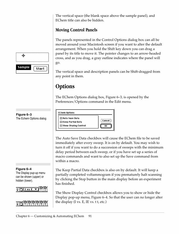
Chapter 6 — Customizing
Figure 6–4 The Display pup-up menu can be shown (upper) or hidden (lower).
The vertical space (the blank space above the sample panel), and EChem title can also be hidden.
Moving Control Panels
The panels represented in the Control Options dialog box can all be moved around your Macintosh screen if you want to alter the default arrangement. When you hold the Shift key down you can drag a panel by its title to move it. The pointer changes to an arrow-headed cross, and as you drag, a gray outline indicates where the panel will go.
The vertical space and description panels can be Shift-dragged from any point in them.
Options
The EChem Options dialog box, Figure 6–3, is opened by the Preferences/Options command in the Edit menu.
The Auto Save Data checkbox will cause the EChem file to be saved immediately after every sweep. It is on by default. You may wish to turn it off if you want to do a succession of sweeps with the minimum
Figure 6–3 The Echem Options dialog
& Automating EChem 91
delay period between each sweep, or if you have set up a series of macro commands and want to also set up the Save command from within a macro.
The Keep Partial Data checkbox is also on by default. It will keep a partially completed voltammogram if you prematurely halt scanning by clicking the Stop button in the main display before an experiment has finished.
The Show Display Control checkbox allows you to show or hide the Display pop-up menu, Figure 6–4. So that the user can no longer alter the display (I vs. E, IE vs. t t, etc.)
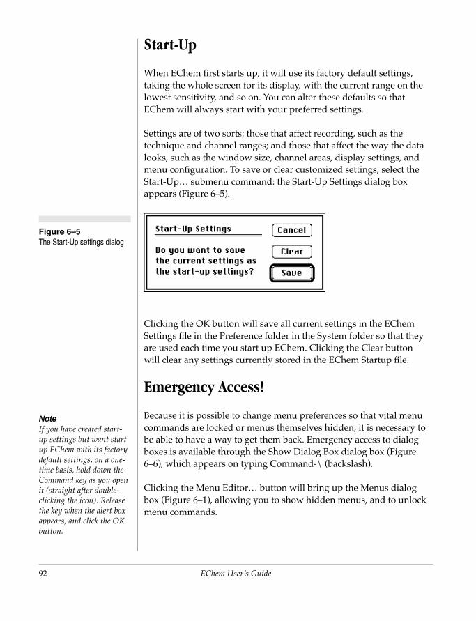
92
Figure 6–5 The Start-Up settings dialog
NoteIf you have created start-up settings but want start up EChem with its factory default settings, on a one-time basis, hold down the Command key as you open it (straight after double-clicking the icon). Release the key when the alert box appears, and click the OK button.
Start-Up
When EChem first starts up, it will use its factory default settings, taking the whole screen for its display, with the current range on the lowest sensitivity, and so on. You can alter these defaults so that EChem will always start with your preferred settings.
Settings are of two sorts: those that affect recording, such as the technique and channel ranges; and those that affect the way the data looks, such as the window size, channel areas, display settings, and menu configuration. To save or clear customized settings, select the Start-Up… submenu command: the Start-Up Settings dialog box appears (Figure 6–5).
Clicking the OK button will save all current settings in the EChem Settings file in the Preference folder in the System folder so that they are used each time you start up EChem. Clicking the Clear button will clear any settings currently stored in the EChem Startup file.
Emergency Access!
EChem User’s Guide
Because it is possible to change menu preferences so that vital menu commands are locked or menus themselves hidden, it is necessary to be able to have a way to get them back. Emergency access to dialog boxes is available through the Show Dialog Box dialog box (Figure 6–6), which appears on typing Command-\ (backslash).
Clicking the Menu Editor… button will bring up the Menus dialog box (Figure 6–1), allowing you to show hidden menus, and to unlock menu commands.
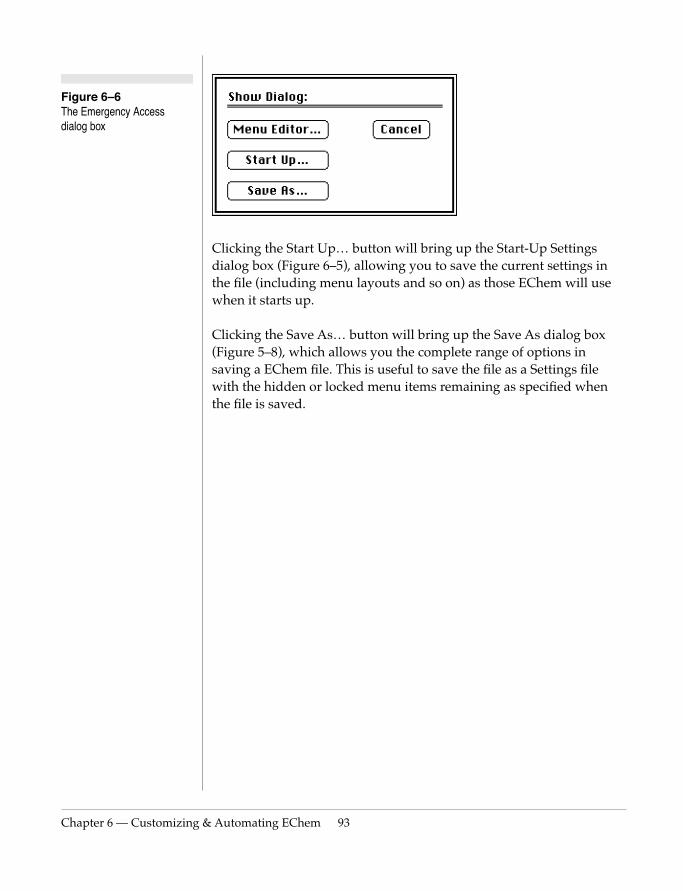
Chapter 6 — Customizing
Figure 6–6 The Emergency Access dialog box
Clicking the Start Up… button will bring up the Start-Up Settings dialog box (Figure 6–5), allowing you to save the current settings in the file (including menu layouts and so on) as those EChem will use when it starts up.
Clicking the Save As… button will bring up the Save As dialog box (Figure 5–8), which allows you the complete range of options in saving a EChem file. This is useful to save the file as a Settings file with the hidden or locked menu items remaining as specified when the file is saved.
& Automating EChem 93
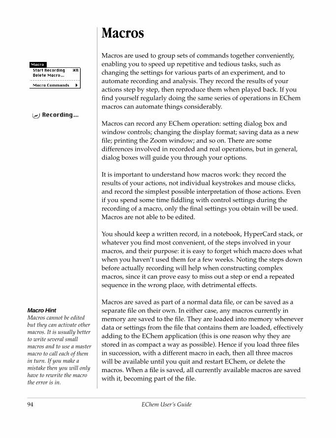
94
Macro HintMacros cannot be edited but they can activate other macros. It is usually better to write several small macros and to use a master macro to call each of them in turn. If you make a mistake then you will only have to rewrite the macro the error is in.
MacrosMacros are used to group sets of commands together conveniently, enabling you to speed up repetitive and tedious tasks, such as changing the settings for various parts of an experiment, and to automate recording and analysis. They record the results of your actions step by step, then reproduce them when played back. If you find yourself regularly doing the same series of operations in EChem macros can automate things considerably.
Macros can record any EChem operation: setting dialog box and window controls; changing the display format; saving data as a new file; printing the Zoom window; and so on. There are some differences involved in recorded and real operations, but in general, dialog boxes will guide you through your options.
It is important to understand how macros work: they record the results of your actions, not individual keystrokes and mouse clicks, and record the simplest possible interpretation of those actions. Even if you spend some time fiddling with control settings during the recording of a macro, only the final settings you obtain will be used. Macros are not able to be edited.
You should keep a written record, in a notebook, HyperCard stack, or whatever you find most convenient, of the steps involved in your macros, and their purpose: it is easy to forget which macro does what when you haven’t used them for a few weeks. Noting the steps down before actually recording will help when constructing complex macros, since it can prove easy to miss out a step or end a repeated
EChem User’s Guide
sequence in the wrong place, with detrimental effects.
Macros are saved as part of a normal data file, or can be saved as a separate file on their own. In either case, any macros currently in memory are saved to the file. They are loaded into memory whenever data or settings from the file that contains them are loaded, effectively adding to the EChem application (this is one reason why they are stored in as compact a way as possible). Hence if you load three files in succession, with a different macro in each, then all three macros will be available until you quit and restart EChem, or delete the macros. When a file is saved, all currently available macros are saved with it, becoming part of the file.
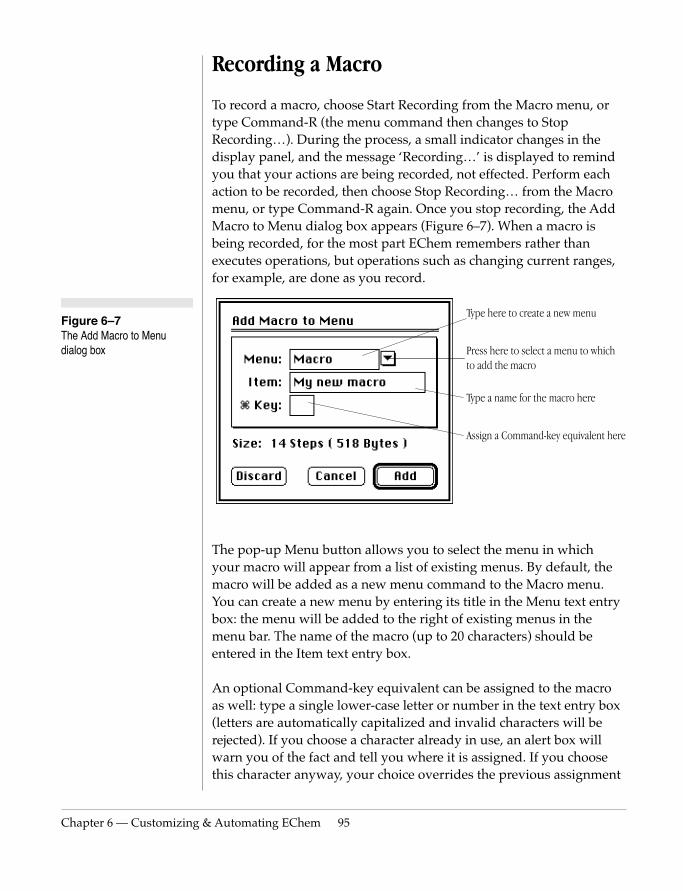
Chapter 6 — Customizing
Figure 6–7 The Add Macro to Menu dialog box
Recording a Macro
To record a macro, choose Start Recording from the Macro menu, or type Command-R (the menu command then changes to Stop Recording…). During the process, a small indicator changes in the display panel, and the message ‘Recording…’ is displayed to remind you that your actions are being recorded, not effected. Perform each action to be recorded, then choose Stop Recording… from the Macro menu, or type Command-R again. Once you stop recording, the Add Macro to Menu dialog box appears (Figure 6–7). When a macro is being recorded, for the most part EChem remembers rather than executes operations, but operations such as changing current ranges, for example, are done as you record.
The pop-up Menu button allows you to select the menu in which your macro will appear from a list of existing menus. By default, the
Type a name for the macro here
Press here to select a menu to which to add the macro
Assign a Command-key equivalent here
Type here to create a new menu
& Automating EChem 95
macro will be added as a new menu command to the Macro menu. You can create a new menu by entering its title in the Menu text entry box: the menu will be added to the right of existing menus in the menu bar. The name of the macro (up to 20 characters) should be entered in the Item text entry box.
An optional Command-key equivalent can be assigned to the macro as well: type a single lower-case letter or number in the text entry box (letters are automatically capitalized and invalid characters will be rejected). If you choose a character already in use, an alert box will warn you of the fact and tell you where it is assigned. If you choose this character anyway, your choice overrides the previous assignment
96
and the Command-key equivalent will only work for (and appear beside) the menu command that you have just created.
The Size indicator tells you the number of steps recorded (useful if you can’t remember which step you are up to in the middle of a complex macro), and the memory taken by the macro, so far. The amount of memory used depends on the complexity of the procedure. Click the Discard button to discard the macro you have just recorded. Click the Cancel button to continue recording more steps in the macro. Click the Add button to add the macro to the bottom of the selected menu; the Add button is only active and undimmed when the macro is named and a menu is chosen.
Until you save the file, the macro exists only in memory and is not permanently stored. If you open another file and save that, the macro (and all other currently available macros) will become part of the new file. When you quit EChem, you will not be asked to save changes if you have created new or altered existing macros. So it is a good idea to save the file each time you create a macro (or save it as various macro files).
Playing a Macro
Once assigned a name and location, macros act much as if they were menu commands. Select them from their menu or type their Command-key equivalent to use them. While a macro plays, the title of the menu in which it resides is highlighted, and no other functions can be performed within EChem, nor can one switch to another application and leave EChem in the background. To stop a macro
EChem User’s Guide
playing, hold down the Command key and press Period (.). The macro will stop at its current step.
Deleting a Macro
To delete existing macros, choose the Delete Macro menu command in the Macro menu which brings up the Delete Macro dialog box (Figure 6–8).
A scrolling list displays the name of the menu that the macro is in, a colon, and the name of the macro, for all available macros. To delete a macro, select it and click the Delete button. To delete multiple macros,

Chapter 6 — Customizing
Figure 6–8 The Delete Macro dialog box
Shift-click or Shift-drag to select contiguous macros, or Command-click (or Control-click) to select or deselect multiple macros individually. The dialog box will close and the macro or macros will be gone. As a shortcut, double-click a macro to delete it and close the dialog box in one step.
As was mentioned, when a file is saved, all currently available macros are saved with it. When you delete a macro, you delete it from memory. If the macro is part of the current file, it is permanently deleted from that file only when the file is saved. Copies of the same macro that are part of other files will not be deleted.
Macros That Call Other Macros
Once a macro has been created, it can then be used by other macros that you create. When constructing multistep procedures it is usually
& Automating EChem 97
best to call a series of small macros from a single master macro. Macros can be nested up to ten deep. An alert box will appear during the playing of your macros if the combination of macros becomes too recursive.
If a macro is called by another macro, EChem will warn you if you attempt to delete it. If you delete it without replacing it then, when the deleted macro is called, an alert box will tell you that it cannot be found.

98
Options When Recording Macros
Operations involving files and dialog boxes can be made to behave in different ways when playing macros, depending on whether you want to do the same thing all the time, allow user modification, and so on.
Changing Dialog Box Settings
Macros can be used to change dialog box settings to the values specified when you record the macro, or to open a dialog box for the user to change settings when the macro is played.
If you want a macro that changes the settings in a dialog box, then select the dialog box as you would normally while recording the macro. Change the settings, and then click OK in the dialog box. (If you click Cancel, the changes made in the dialog box will be ignored.) When playing the macro, the settings are changed without displaying the dialog box.
If you want a macro that opens a dialog box for the user to change settings when the macro is played, hold down the Option key when selecting the command that shows the dialog box while recording the macro, then click the OK button. Do not make any setting changes. When you play back the macro, the dialog box is displayed so that its settings can be changed by the user. Clicking the OK or Cancel buttons in the dialog box will allow the macro to continue, with the user-defined settings or the original settings respectively.
EChem User’s Guide
When changing control values in dialog boxes, absolute values are recorded, not relative changes. For example, if you move a scroll bar that increases potential by 50%, from 1V to 1.5 V, the new potential (1.5 V) is recorded, not the change in voltage (+0.5 V) or the percentage change in potential (+50%).
Starting Sampling
Macros can be used to control when sampling starts and stops: you simply click the Start button when recording the macro, and EChem will start sampling at the appropriate point when the macro is played.

Chapter 6 — Customizing
Figure 6–9 The Macro Open dialog box
Opening Files
A macro can be used to open the same file each time it is played, or to allow the user to choose which file to open. To open a particular file with a macro, choose Open… from the File menu while the macro is being recorded: the Macro Open directory dialog box is displayed (Figure 6–9).
To allow the user to choose which file is to be opened when the macro is played, press the Option key when selecting the Open… command while recording the macro. The Open directory dialog box will be displayed when the macro is played.
& Automating EChem 99
When opening the same file each time, the full hierarchical file name (the ‘pathname’) of the file, from the disk through any number of folders, is noted. If the file has been moved (or deleted) since the macro was recorded, then EChem searches in the most recently used folder and in the same folder as EChem. If the file is in neither of these locations, an alert box lets you know that EChem cannot find the file, and the Open directory dialog box is displayed to allow you to find it yourself. If you choose a different file at this stage, it will be opened instead and if you click the Cancel button, the macro will abort.
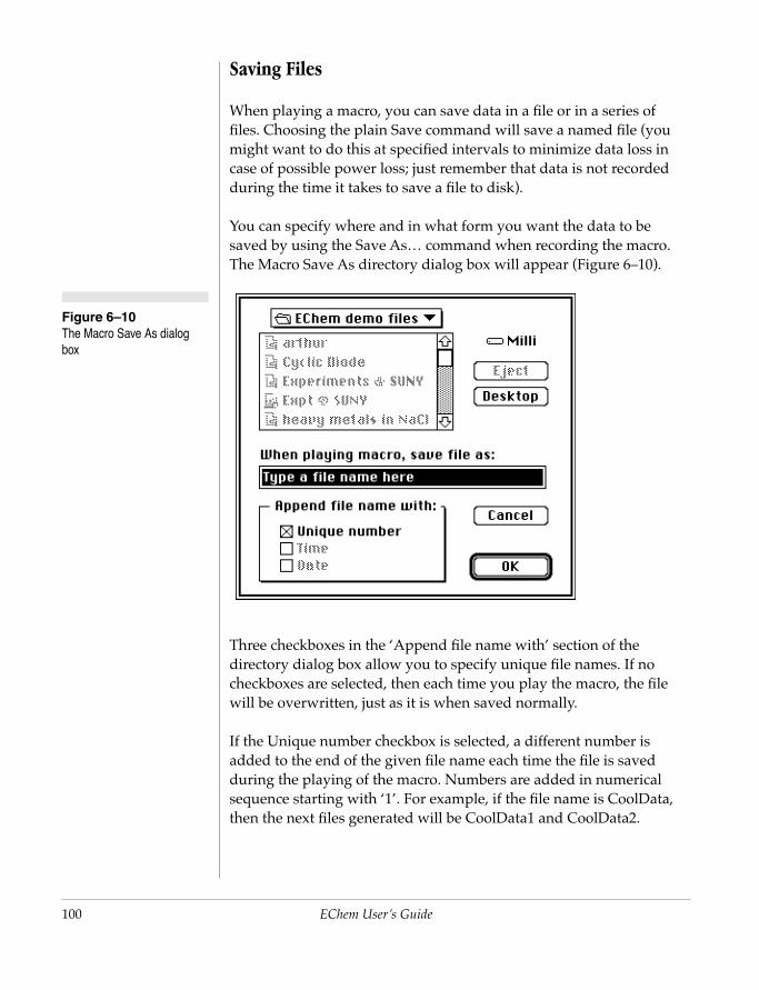
100
Figure 6–10 The Macro Save As dialog box
Saving Files
When playing a macro, you can save data in a file or in a series of files. Choosing the plain Save command will save a named file (you might want to do this at specified intervals to minimize data loss in case of possible power loss; just remember that data is not recorded during the time it takes to save a file to disk).
You can specify where and in what form you want the data to be saved by using the Save As… command when recording the macro. The Macro Save As directory dialog box will appear (Figure 6–10).
EChem User’s Guide
Three checkboxes in the ‘Append file name with’ section of the directory dialog box allow you to specify unique file names. If no checkboxes are selected, then each time you play the macro, the file will be overwritten, just as it is when saved normally.
If the Unique number checkbox is selected, a different number is added to the end of the given file name each time the file is saved during the playing of the macro. Numbers are added in numerical sequence starting with ‘1’. For example, if the file name is CoolData, then the next files generated will be CoolData1 and CoolData2.
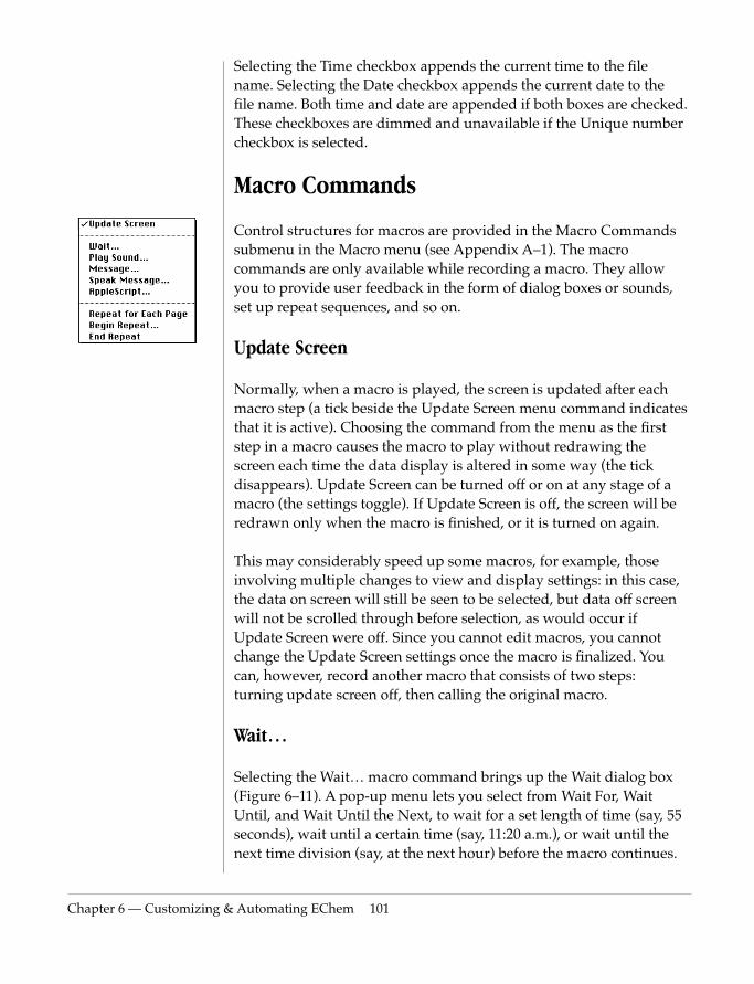
Chapter 6 — Customizing
Selecting the Time checkbox appends the current time to the file name. Selecting the Date checkbox appends the current date to the file name. Both time and date are appended if both boxes are checked. These checkboxes are dimmed and unavailable if the Unique number checkbox is selected.
Macro Commands
Control structures for macros are provided in the Macro Commands submenu in the Macro menu (see Appendix A–1). The macro commands are only available while recording a macro. They allow you to provide user feedback in the form of dialog boxes or sounds, set up repeat sequences, and so on.
Update Screen
Normally, when a macro is played, the screen is updated after each macro step (a tick beside the Update Screen menu command indicates that it is active). Choosing the command from the menu as the first step in a macro causes the macro to play without redrawing the screen each time the data display is altered in some way (the tick disappears). Update Screen can be turned off or on at any stage of a macro (the settings toggle). If Update Screen is off, the screen will be redrawn only when the macro is finished, or it is turned on again.
This may considerably speed up some macros, for example, those involving multiple changes to view and display settings: in this case, the data on screen will still be seen to be selected, but data off screen will not be scrolled through before selection, as would occur if
& Automating EChem 101
Update Screen were off. Since you cannot edit macros, you cannot change the Update Screen settings once the macro is finalized. You can, however, record another macro that consists of two steps: turning update screen off, then calling the original macro.
Wait…
Selecting the Wait… macro command brings up the Wait dialog box (Figure 6–11). A pop-up menu lets you select from Wait For, Wait Until, and Wait Until the Next, to wait for a set length of time (say, 55 seconds), wait until a certain time (say, 11:20 a.m.), or wait until the next time division (say, at the next hour) before the macro continues.
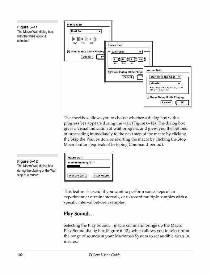
102
Figure 6–12 The Macro Wait dialog box during the playing of the Wait step of a macro
Figure 6–11 The Macro Wait dialog box, with the three options selected
The checkbox allows you to choose whether a dialog box with a progress bar appears during the wait (Figure 6–12). The dialog box gives a visual indication of wait progress, and gives you the options of proceeding immediately to the next step of the macro by clicking the Skip the Wait button, or aborting the macro by clicking the Stop Macro button (equivalent to typing Command-period).
EChem User’s Guide
This feature is useful if you want to perform some steps of an experiment at certain intervals, or to record multiple samples with a specific interval between samples.
Play Sound…
Selecting the Play Sound… macro command brings up the Macro Play Sound dialog box (Figure 6–12), which allows you to select from the range of sounds in your Macintosh System to set audible alerts in macros.
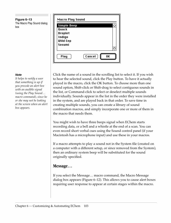
Chapter 6 — Customizing
NoteIt helps to notify a user that something is up if you precede an alert box with an audible signal (using the Play Sound… macro command), since he or she may not be looking at the screen when an alert box appears.
Figure 6–13 The Macro Play Sound dialog box
Click the name of a sound in the scrolling list to select it. If you wish to hear the selected sound, click the Play button. To have it actually played in the macro, click the OK button. To choose more than one sound option, Shift-click or Shift-drag to select contiguous sounds in the list, or Command-click to select or deselect multiple sounds individually. Sounds appear in the list in the order they were installed in the system, and are played back in that order. To save time in creating multiple sounds, you can create a library of sound combination macros, and simply incorporate one or more of them in the macro that needs them.
You might wish to have three beeps signal when EChem starts recording data, or a bell and a whistle at the end of a scan. You can even record short verbal cues using the Sound control panel (if your Macintosh has a microphone input) and use these in your macros.
& Automating EChem 103
If a macro attempts to play a sound not in the System file (created on a computer with a different setup, or since removed from the System), then an ordinary system beep will be substituted for the sound originally specified.
Message…
If you select the Message… macro command, the Macro Message dialog box appears (Figure 6–12). This allows you to cause alert boxes requiring user response to appear at certain stages within the macro.

104
Figure 6–14 The Macro Message dialog box
NoteThe Speak Message command is only available on Macintosh systems.
You can type in the message of your choice (up to 255 characters). The dialog box produced will have an OK button, and if the checkbox at the top is highlighted, a ‘Cancel’ button as well (for exiting the macro).
There are four choices of icon: the default shape (a hand) is highlighted with a heavy border. Click one of the icon buttons to choose it. You can use the icons to indicate the urgency of an important message (hand, exclamation mark, and face, in order of decreasing urgency), and the EChem icon for general messages which indicate EChem’s state. Click the OK button when you have chosen an icon and typed in the message.
Speak Message…
If you select the Speak Message… macro command, the Speak Message dialog box appears (Figure 6–15). Using it, you can give
EChem User’s Guide
spoken messages in macros, if your Macintosh has speech abilities. Type in the phonetic equivalents to allow non-English words to be spoken. After the message is spoken, the macro carries out subsequent steps.
You can type in the message of your choice (up to 255 characters). If the Macintosh on which the macro plays has no speech abilities then, if the checkbox is off, a standard system beep will be used in place of the spoken message. If the checkbox is on, an alert box appears, just as if the Macro message dialog box were used: this will stop the macro until its OK button is clicked.

Chapter 6 — Customizing
Figure 6–15 The Speak Message dialog box
Figure 6–16 The Begin Repeat dialog box
The volume at which the message is spoken can either be the default system volume set in the Sound control panel, or can be set independently to any of the sound levels, from 1 to 7, available in the Sound control panel, by clicking or pressing the arrow controls.
Begin Repeat
The Begin Repeat macro command brings up the Begin Repeat dialog box (Figure 6–16). This is used to repeat groups of steps in a macro. You may repeat any group of commands up to 100,000 times. This could be used, for example, to set up sampling at staggered intervals overnight. For each Begin Repeat you should specify an End Repeat. If you do not specify enough End Repeats, they are automatically added when you select Stop Recording…, but if you have a complex macro, the repeated sequences might not end up in the right places. Writing down the macro before recording it will help avoid such problems.
& Automating EChem 105
Repeat for Each Page
This macro command allows you to perform some operation on each overlaid page of data in turn in the EChem file. The blank (last) page, and pages not in the overlay, will be ignored.
106
NoteThe AppleScript command is only available on Macintosh systems.
When this macro command plays, it will go through the EChem file and display each page it operates upon, which may take a while: turn off the Update Screen command to avoid this. As with the Begin Repeat macro command, you should specify an End Repeat after the instructions you want performed in the repeated sequence.
End Repeat
Each Begin Repeat or Repeat for Each Page macro you specify should be paired with an End Repeat. If you do not specify enough End Repeats, they are automatically added when you select Stop Recording…, but if you have a complex macro, the repeated sequences might not end up in the right places. Writing down the macro before recording it will help avoid such problems.
AppleScript…
This macro command allows you to insert an AppleScript as a macro step. AppleScript is a scripting language for automating tasks, and controlling applications and their interactions through Apple events. To use it, you must have AppleScript installed on your Macintosh. On selecting the AppleScript… macro command, the AppleScript from Macro dialog box appears. You will also need to be familiar with using AppleScript.
For more information read the AppleScript section of your Scope User’s Guide. The EChem software has similar capability.
EChem User’s Guide

EChem
User’s Guide7
C H A P T E R S E V E NEChem Techniques
This chapter describes each of the items in the EChem Techniques
menu and the experiments that can be performed. Unnecessary
Techniques can be deleted from the menu by use of the Menu Editor
(discussed in Chapter 6).
Commonly performed experiments can be quickly configured with
the technique and exact parameters (scan rate, upper and lower
potential limits, pulse duration etc.) by the use of Settings Files or
Macros (Chapter 6).
In addition, other electrochemical experiments can be performed with
the Chart and Scope software, and these techniques are discussed in
107
Chapter 8. Chapter 8 also describes the use of EChem for AC
voltammetry and AC cyclic voltammetry.
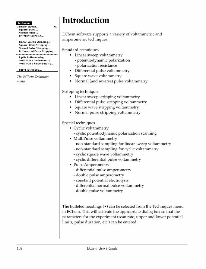
108
The EChem Technique menu
IntroductionEChem software supports a variety of voltammetric and amperometric techniques:
Standard techniques• Linear sweep voltammetry
- potentiodynamic polarization- polarization resistance
• Differential pulse voltammetry• Square wave voltammetry• Normal (and reverse) pulse voltammetry
Stripping techniques• Linear sweep stripping voltammetry• Differential pulse stripping voltammetry• Square wave stripping voltammetry• Normal pulse stripping voltammetry
Special techniques• Cyclic voltammetry
- cyclic potentiodynamic polarization scanning• MultiPulse voltammetry
- non-standard sampling for linear sweep voltammetry- non-standard sampling for cyclic voltammetry- cyclic square wave voltammetry- cyclic differential pulse voltammetry
• Pulse Amperometry- differential pulse amperometry
EChem User’s Guide
- double pulse amperometry- constant potential electrolysis- differential normal pulse voltammetry- double pulse voltammetry
The bulleted headings (•) can be selected from the Techniques menu in EChem. This will activate the appropriate dialog box so that the parameters for the experiment (scan rate, upper and lower potential limits, pulse duration, etc.) can be entered.
Chapter 7 — EChem Techn
All ‘Stripping’ and ‘Special’ techniques include controls that enable a pre-scan deposition and a post-scan cleaning potential to be applied.
Multi Pulse Voltammetry is a general purpose technique allowing you to define any potential waveform that may be constructed from a combination of a stepped ramp with one or two pulses superimposed on each step. Up to four current signal sampling periods may be defined for each step/pulse cycle. This technique can also be used to set up nonstandard linear sweep, cyclic, square wave and differential pulse voltammetry experiments where the current signal is sampled at non standard times. It can also be used to perform cyclic square wave and cyclic differential pulse voltammetry.
The ‘Pulse Amperometry’ technique allows a fixed potential to be set with up to two pulses to be performed over a pre-set interval. The potential/pulse interval can be repeated up to 16000 times, to create a continuous scan.
Support for polarography experiments with a dropping mercury electrode is provided by means of synchronized TTL pulse signals (available on PowerLab S series units only).
Each of these techniques is discussed in greater detail in the following sections.
Other techniques, which can be performed with Chart and Scope software, are discussed in Chapter 8.
EChem software can also be used in conjunction with an AC waveform generator and lock-in amplifier to drive a potentiostat for
iques 109
AC voltammetry and AC cyclic voltammetry (also discussed in Chapter 8).

110
Figure 7–1 Typical potential/time profile of a voltammetric ramp
General ConsiderationsVoltammetric experiments involve measuring the current signal while the potential difference between the working and reference electrode is varied. Results are usually presented as a plot of current versus potential.
Amperometric techniques use a fixed base potential, i.e. they have a scan rate of 0 V/s. However pulses may be superimposed on the base potential. The results are usually plotted as current signal versus time.
The Voltammetric Ramp
Voltammetric techniques require that the potential between the reference and working electrodes be increased or decreased at a constant rate. If the potential at the electrode is plotted against time then the resulting graph has the appearance of a smooth ramp(Figure 7–1).
Time
Pot
entia
l
EChem User’s Guide
With digital instrumentation, such as the PowerLab system, the ramp actually consists of a series of discrete steps (and thus is often called a staircase or stepped ramp) defined by the step width (ts) and step height (Es) as shown in Figure 7–2.
The coarseness of this staircase is a function of the step width (ts) and step height (Es). Step widths should be chosen to keep the step height to a minimum (generally the step height should be less than 10 mV with 1 or 2 mV being ideal). Then minimum step width and height available depend on the potential range and sampling speed selected.

Chapter 7 — EChem Techn
Figure 7–2 The digitally generated ‘staircase’ ramp
Table 7–1 Dependence of Step Height resolution on selected Potential Range. The Step Height at any range setting must be a multiple of the resolution.
Potential Range Step Height resolution
±1 V 0.5 mV
±2 V 1.0 mV
±5 V 2.5 mV
Table 7–2 Dependence of time base on selected Sampling Speed. The Step Width, Sampling Period, and Pulse Width at any speed setting must
Pot
entia
l
Time
Staircase ramp
Resttime t s
E s
iques 111
be multiples of the time base.
Sampling speed Time Base
100 Hz 10 ms
400 Hz 2.5 ms
1 kHz 1 ms
4 kHz 0.25 ms
10 kHz 0.1 ms
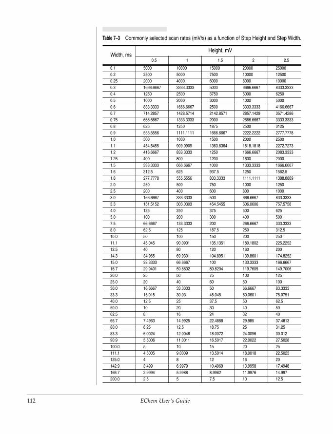
112
Table 7–3 Commonly selected scan rates (mV/s) as a function of Step Height and Step Width.
Width, msHeight, mV
0.5 1 1.5 2 2.5
0.1 5000 10000 15000 20000 250000.2 2500 5000 7500 10000 125000.25 2000 4000 6000 8000 100000.3 1666.6667 3333.3333 5000 6666.6667 8333.33330.4 1250 2500 3750 5000 62500.5 1000 2000 3000 4000 50000.6 833.3333 1666.6667 2500 3333.3333 4166.66670.7 714.2857 1428.5714 2142.8571 2857.1429 3571.42860.75 666.6667 1333.3333 2000 2666.6667 3333.33330.8 625 1250 1875 2500 31250.9 555.5556 1111.1111 1666.6667 2222.2222 2777.77781.0 500 1000 1500 2000 25001.1 454.5455 909.0909 1363.6364 1818.1818 2272.72731.2 416.6667 833.3333 1250 1666.6667 2083.33331.25 400 800 1200 1600 20001.5 333.3333 666.6667 1000 1333.3333 1666.66671.6 312.5 625 937.5 1250 1562.51.8 277.7778 555.5556 833.3333 1111.1111 1388.88892.0 250 500 750 1000 12502.5 200 400 600 800 10003.0 166.6667 333.3333 500 666.6667 833.33333.3 151.5152 303.0303 454.5455 606.0606 757.57584.0 125 250 375 500 6255.0 100 200 300 400 5007.5 66.6667 133.3333 200 266.6667 333.33338.0 62.5 125 187.5 250 312.510.0 50 100 150 200 25011.1 45.045 90.0901 135.1351 180.1802 225.225212.5 40 80 120 160 20014.3 34.965 69.9301 104.8951 139.8601 174.825215.0 33.3333 66.6667 100 133.3333 166.666716.7 29.9401 59.8802 89.8204 119.7605 149.700620.0 25 50 75 100 125
EChem User’s Guide
25.0 20 40 60 80 10030.0 16.6667 33.3333 50 66.6667 83.333333.3 15.015 30.03 45.045 60.0601 75.075140.0 12.5 25 37.5 50 62.550.0 10 20 30 40 5062.5 8 16 24 32 4066.7 7.4963 14.9925 22.4888 29.985 37.481380.0 6.25 12.5 18.75 25 31.2583.3 6.0024 12.0048 18.0072 24.0096 30.01290.9 5.5006 11.0011 16.5017 22.0022 27.5028100.0 5 10 15 20 25111.1 4.5005 9.0009 13.5014 18.0018 22.5023125.0 4 8 12 16 20142.9 3.499 6.9979 10.4969 13.9958 17.4948166.7 2.9994 5.9988 8.9982 11.9976 14.997200.0 2.5 5 7.5 10 12.5
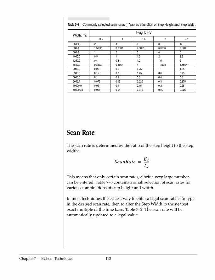
Chapter 7 — EChem Techn
Scan Rate
The scan rate is determined by the ratio of the step height to the step width:
This means that only certain scan rates, albeit a very large number,
250.0 2 4 6 8 10333.3 1.5002 3.0003 4.5005 6.0006 7.5008500.0 1 2 3 4 51000.0 0.5 1 1.5 2 2.51250.0 0.4 0.8 1.2 1.6 21500.0 0.3333 0.6667 1 1.3333 1.66672000.0 0.25 0.5 0.75 1 1.253333.3 0.15 0.3 0.45 0.6 0.755000.0 0.1 0.2 0.3 0.4 0.56666.7 0.075 0.15 0.225 0.3 0.37510000.0 0.05 0.1 0.15 0.2 0.25100000.0 0.005 0.01 0.015 0.02 0.025
Table 7–3 Commonly selected scan rates (mV/s) as a function of Step Height and Step Width.
Width, msHeight, mV
0.5 1 1.5 2 2.5
ScanRateEsts------=
iques 113
can be entered. Table 7–3 contains a small selection of scan rates for various combinations of step height and width.
In most techniques the easiest way to enter a legal scan rate is to type in the desired scan rate, then to alter the Step Width to the nearest exact multiple of the time base, Table 7–2. The scan rate will be automatically updated to a legal value.
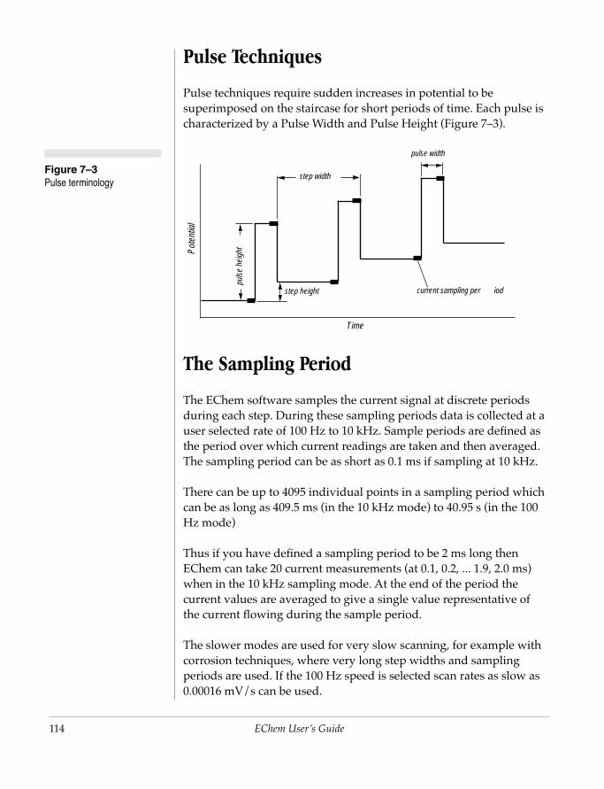
114
Figure 7–3 Pulse terminology
Pulse Techniques
Pulse techniques require sudden increases in potential to be superimposed on the staircase for short periods of time. Each pulse is characterized by a Pulse Width and Pulse Height (Figure 7–3).
The Sampling Period
The EChem software samples the current signal at discrete periods during each step. During these sampling periods data is collected at a user selected rate of 100 Hz to 10 kHz. Sample periods are defined as the period over which current readings are taken and then averaged. The sampling period can be as short as 0.1 ms if sampling at 10 kHz.
There can be up to 4095 individual points in a sampling period which
puls
e he
ight
step width
step height
pulse width
current sampling per iod
Pot
entia
l
Time
EChem User’s Guide
can be as long as 409.5 ms (in the 10 kHz mode) to 40.95 s (in the 100 Hz mode)
Thus if you have defined a sampling period to be 2 ms long then EChem can take 20 current measurements (at 0.1, 0.2, ... 1.9, 2.0 ms) when in the 10 kHz sampling mode. At the end of the period the current values are averaged to give a single value representative of the current flowing during the sample period.
The slower modes are used for very slow scanning, for example with corrosion techniques, where very long step widths and sampling periods are used. If the 100 Hz speed is selected scan rates as slow as 0.00016 mV/s can be used.
Chapter 7 — EChem Techn
By selecting a sample period of 20 ms or 16.7 ms (for 50 or 60 Hz mains) you can dramatically remove main noise from your voltammograms.
When using slower scan rates the sampling period can be set to minimize mains noise. If you are operating on a mains frequency of 50 Hz (Europe, Australia, Chile, Argentina, and most of Africa, Asia) then use sampling periods that are a multiple of 1/50 Hz = 20 ms, i.e. a single mains AC cycle. If you are operating at 60 Hz (North America, South Korea, Taiwan, most of South America, and parts of Japan, Peru and Saudi Arabia, etc.) then make your sample period a multiple of 1/60 Hz ≈ 16.7 ms. This will cause the current data to be sampled over an integral number of mains AC cycles and thus any noise arising from this source will be effectively filtered out.
With most techniques the sampling period is located at the end of the pulse or step. But with the more flexible MultiPulse Voltammetry and Amperometry techniques you may set the sample period to be at the beginning, middle or end of a step or pulse.
The Rest Time
Before data is recorded it is common to bring the working electrode to the initial potential of the applied potential ramp. The potential is then held at this value for a short period of time, the rest time, (usually several seconds or longer) for the current flow to stabilise, and for the solution to settle after stirring.
iques 115
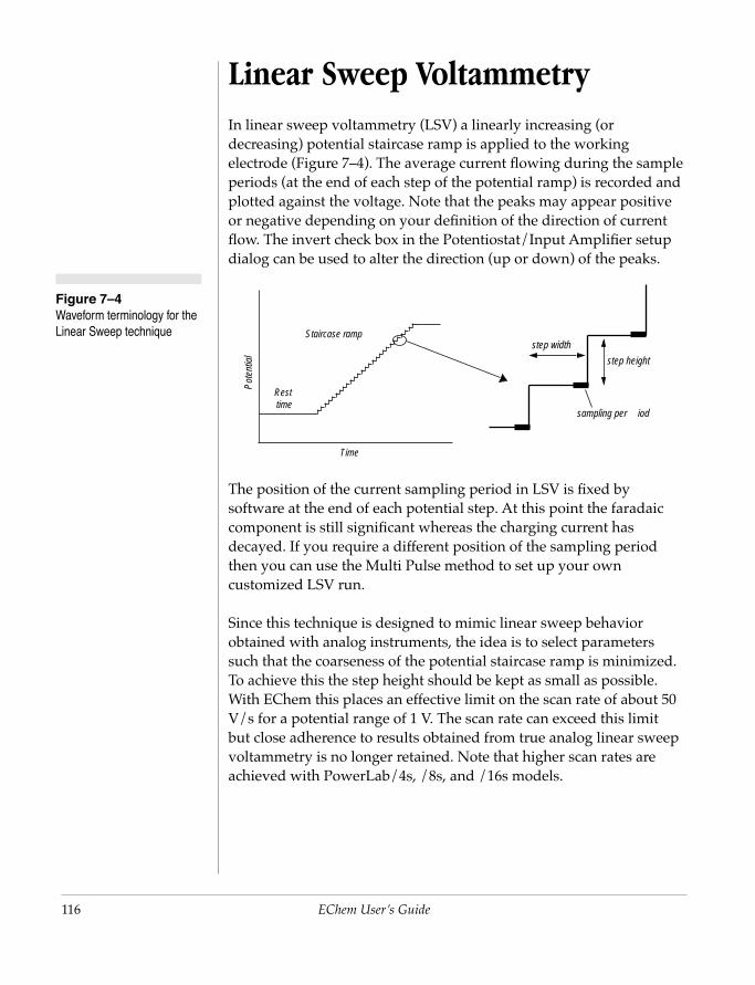
116
Figure 7–4 Waveform terminology for the Linear Sweep technique
Linear Sweep VoltammetryIn linear sweep voltammetry (LSV) a linearly increasing (or decreasing) potential staircase ramp is applied to the working electrode (Figure 7–4). The average current flowing during the sample periods (at the end of each step of the potential ramp) is recorded and plotted against the voltage. Note that the peaks may appear positive or negative depending on your definition of the direction of current flow. The invert check box in the Potentiostat/Input Amplifier setup dialog can be used to alter the direction (up or down) of the peaks.
The position of the current sampling period in LSV is fixed by software at the end of each potential step. At this point the faradaic component is still significant whereas the charging current has decayed. If you require a different position of the sampling period then you can use the Multi Pulse method to set up your own customized LSV run.
Since this technique is designed to mimic linear sweep behavior
Pot
entia
l
Time
Staircase ramp
Resttime
step width
step height
sampling per iod
EChem User’s Guide
obtained with analog instruments, the idea is to select parameters such that the coarseness of the potential staircase ramp is minimized. To achieve this the step height should be kept as small as possible. With EChem this places an effective limit on the scan rate of about 50 V/s for a potential range of 1 V. The scan rate can exceed this limit but close adherence to results obtained from true analog linear sweep voltammetry is no longer retained. Note that higher scan rates are achieved with PowerLab/4s, /8s, and /16s models.
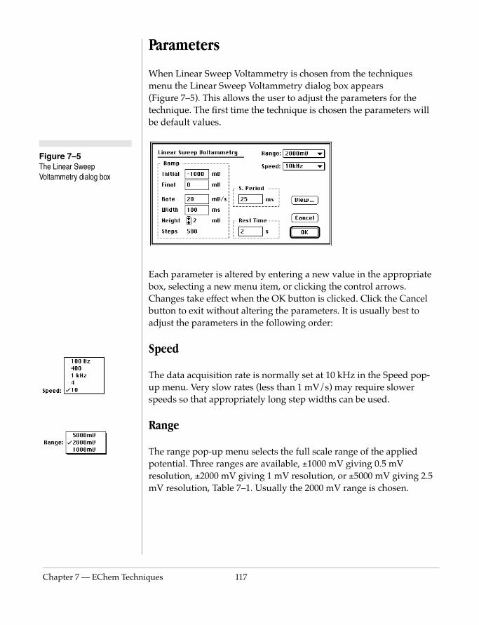
Chapter 7 — EChem Techn
Figure 7–5 The Linear Sweep Voltammetry dialog box
Parameters
When Linear Sweep Voltammetry is chosen from the techniques menu the Linear Sweep Voltammetry dialog box appears (Figure 7–5). This allows the user to adjust the parameters for the technique. The first time the technique is chosen the parameters will be default values.
Each parameter is altered by entering a new value in the appropriate box, selecting a new menu item, or clicking the control arrows. Changes take effect when the OK button is clicked. Click the Cancel button to exit without altering the parameters. It is usually best to adjust the parameters in the following order:
Speed
The data acquisition rate is normally set at 10 kHz in the Speed pop-up menu. Very slow rates (less than 1 mV/s) may require slower speeds so that appropriately long step widths can be used.
iques 117
Range
The range pop-up menu selects the full scale range of the applied potential. Three ranges are available, ±1000 mV giving 0.5 mV resolution, ±2000 mV giving 1 mV resolution, or ±5000 mV giving 2.5 mV resolution, Table 7–1. Usually the 2000 mV range is chosen.
118
(Step) Height
This is the amplitude of each potential step. The minimum step available depends on the selected range, Table 7–1. Values from 0.5 to 2.5 mV are ideal for work where accurate peak positions, heights and areas are required. Values over 5 mV may give insufficient potential resolution, and also lead to excessively high charging currents at macro electrodes, for most voltammetric and pulse techniques.
Initial (Potential)
This is a text box that sets the initial or starting potential of the ramp. This can be chosen anywhere between the limits of the range setting.
Final (Potential)
The potential voltage at which the ramp waveform finishes.This can be chosen anywhere between the limits of the range setting. The final potential may be either more negative than the initial potential (negative scan) or more positive than the initial potential (positive scan).
Steps
The number of steps in the ramp is derived from the initial and final potentials and the step height:
StepsFinalPotential InitialPotential–
StepHeight------------------------------------------------------------------------------------------=
EChem User’s Guide
This number must be an integer. If it is not then you will have to adjust the Upper and/or Lower Limit so that the difference is an exact multiple of the Step Height.
(Scan) Rate
This sets the rate at which the ramp will be generated. Faster scan rates lead to a higher background signal unless a microelectrode is used. This is usually set between 5 and 1000 mV/s for ordinary macro electrodes. The scan rate is the ratio of the step height to the step
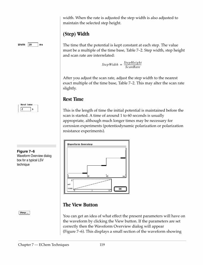
Chapter 7 — EChem Techn
Figure 7–6 Waveform Overview dialog box for a typical LSV technique
width. When the rate is adjusted the step width is also adjusted to maintain the selected step height.
(Step) Width
The time that the potential is kept constant at each step. The value must be a multiple of the time base, Table 7–2. Step width, step height and scan rate are interrelated:
After you adjust the scan rate, adjust the step width to the nearest exact multiple of the time base, Table 7–2. This may alter the scan rate slightly.
Rest Time
This is the length of time the initial potential is maintained before the scan is started. A time of around 1 to 60 seconds is usually appropriate, although much longer times may be necessary for corrosion experiments (potentiodynamic polarization or polarization resistance experiments).
StepWidthStepHeightScanRate
-----------------------------=
iques 119
The View Button
You can get an idea of what effect the present parameters will have on the waveform by clicking the View button. If the parameters are set correctly then the Waveform Overview dialog will appear (Figure 7–6). This displays a small section of the waveform showing

120
the steps and the sampling period (the thick, red, line segments). If the parameters are above the maximum limits or do not make sense then you will see an error dialog describing what is wrong
EChem User’s Guide
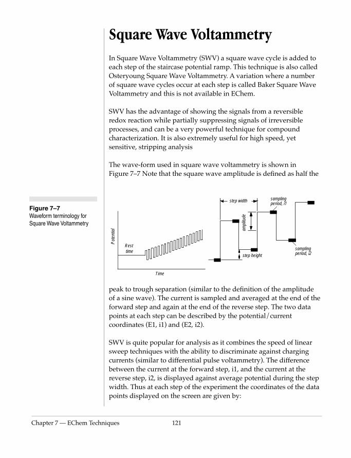
Chapter 7 — EChem Techn
Figure 7–7 Waveform terminology for Square Wave Voltammetry
Square Wave VoltammetryIn Square Wave Voltammetry (SWV) a square wave cycle is added to each step of the staircase potential ramp. This technique is also called Osteryoung Square Wave Voltammetry. A variation where a number of square wave cycles occur at each step is called Baker Square Wave Voltammetry and this is not available in EChem.
SWV has the advantage of showing the signals from a reversible redox reaction while partially suppressing signals of irreversible processes, and can be a very powerful technique for compound characterization. It is also extremely useful for high speed, yet sensitive, stripping analysis
The wave-form used in square wave voltammetry is shown in Figure 7–7 Note that the square wave amplitude is defined as half the
peak to trough separation (similar to the definition of the amplitude
Pot
entia
l
Time
Resttime
step width
step heightsamplingperiod, i2
ampl
itude
samplingperiod, i1
iques 121
of a sine wave). The current is sampled and averaged at the end of the forward step and again at the end of the reverse step. The two data points at each step can be described by the potential/current coordinates (E1, i1) and (E2, i2).
SWV is quite popular for analysis as it combines the speed of linear sweep techniques with the ability to discriminate against charging currents (similar to differential pulse voltammetry). The difference between the current at the forward step, i1, and the current at the reverse step, i2, is displayed against average potential during the step width. Thus at each step of the experiment the coordinates of the data points displayed on the screen are given by:

122
Figure 7–8 The Data Selection dialog box.
([i1-i2], [E1+E2]/2)
The actual values of the two currents, i1 and i2 are stored in the arrays of these names and can be viewed separately by choosing Sampling Display in the Display menu, to present the dialog in Figure 7–8.
The default settings for SWV displays i1–i2 (i3 and i4 are not used for Square Wave Voltammetry). Selecting ‘i2 Minus Nothing’ would change the graph on display so that you would see the current values at the top of each pulse.
You may occasionally find that a SWV run gives you small peaks and that on attempting to run the experiment at a slightly higher gain you find that much of the signal is off scale. Remember that the default display is i1–i2, i.e. the difference between the current values in i1 and i2. It is possible that the arrays i1 and i2 contain many large current values and so need to be recorded on low gain settings to be on scale. You can check that this is so by using the Sampling Display command. If corresponding values in i1 and i2 are both large and nearly equal then the difference, i1–i2 will be small but you will not be able to select higher gains to collect the data.
EChem User’s Guide
Parameters
When Square Wave Voltammetry is chosen from the techniques menu the Square Wave Voltammetry dialog box appears (Figure 7–9). Suitable parameters can be entered in the relevant spaces to alter the technique as needed for the experiment being conducted.
Changes take effect when the OK button is clicked. Click the Cancel button to exit without saving.
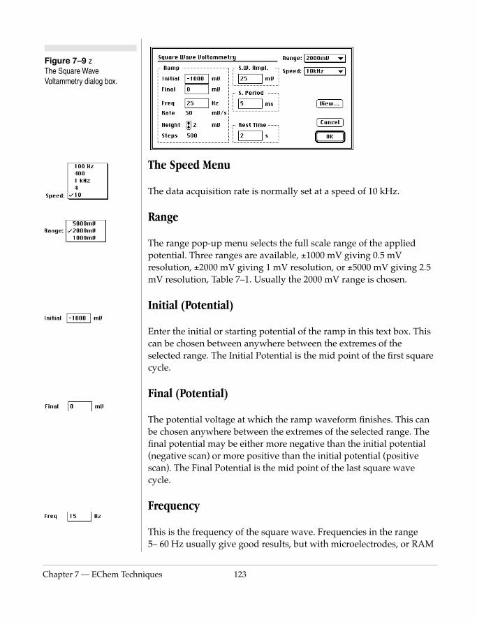
Chapter 7 — EChem Techn
Figure 7–9 zThe Square Wave Voltammetry dialog box.
The Speed Menu
The data acquisition rate is normally set at a speed of 10 kHz.
Range
The range pop-up menu selects the full scale range of the applied potential. Three ranges are available, ±1000 mV giving 0.5 mV resolution, ±2000 mV giving 1 mV resolution, or ±5000 mV giving 2.5 mV resolution, Table 7–1. Usually the 2000 mV range is chosen.
Initial (Potential)
Enter the initial or starting potential of the ramp in this text box. This can be chosen between anywhere between the extremes of the selected range. The Initial Potential is the mid point of the first square cycle.
Final (Potential)
iques 123
The potential voltage at which the ramp waveform finishes. This can be chosen anywhere between the extremes of the selected range. The final potential may be either more negative than the initial potential (negative scan) or more positive than the initial potential (positive scan). The Final Potential is the mid point of the last square wave cycle.
Frequency
This is the frequency of the square wave. Frequencies in the range 5– 60 Hz usually give good results, but with microelectrodes, or RAM
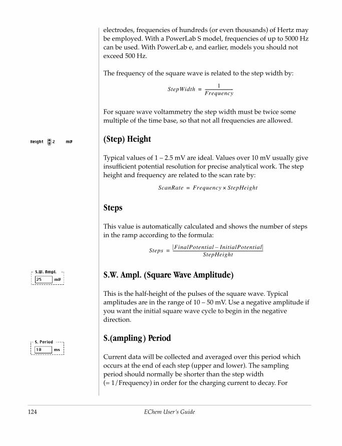
124
electrodes, frequencies of hundreds (or even thousands) of Hertz may be employed. With a PowerLab S model, frequencies of up to 5000 Hz can be used. With PowerLab e, and earlier, models you should not exceed 500 Hz.
The frequency of the square wave is related to the step width by:
For square wave voltammetry the step width must be twice some multiple of the time base, so that not all frequencies are allowed.
(Step) Height
Typical values of 1 – 2.5 mV are ideal. Values over 10 mV usually give insufficient potential resolution for precise analytical work. The step height and frequency are related to the scan rate by:
Steps
This value is automatically calculated and shows the number of steps in the ramp according to the formula:
S.W. Ampl. (Square Wave Amplitude)
StepWidth1
Frequency----------------------------=
ScanRate Frequency StepHeight×=
StepsFinalPotential InitialPotential–
StepHeight------------------------------------------------------------------------------------------=
EChem User’s Guide
This is the half-height of the pulses of the square wave. Typical amplitudes are in the range of 10 – 50 mV. Use a negative amplitude if you want the initial square wave cycle to begin in the negative direction.
S.(ampling) Period
Current data will be collected and averaged over this period which occurs at the end of each step (upper and lower). The sampling period should normally be shorter than the step width (= 1/Frequency) in order for the charging current to decay. For

Chapter 7 — EChem Techn
Figure 7–10 Waveform Overview for a typical Square Wave Voltammetry technique
example at a frequency of 25 Hz the step width is 40 ms. Therefore the sampling period should be set to 40 ms or less (preferably 16.7 or 20 ms to minimize mains 60 Hz or 50 Hz noise interference).
Rest Time
This is the length of time the initial potential is maintained before the scan is started. A time of around 1 to 60 seconds is usually appropriate.
The View button
The quickest way to determine if the parameters you have set will work is to click the view button. If the parameters you have set are logically consistent then the Waveform overview window will appear (Figure 7–10) with a representation of the potential waveform. If for any reason the values you have set are out of range, or otherwise inappropriate, you will be prompted by a dialog box telling you what the problem is.
iques 125
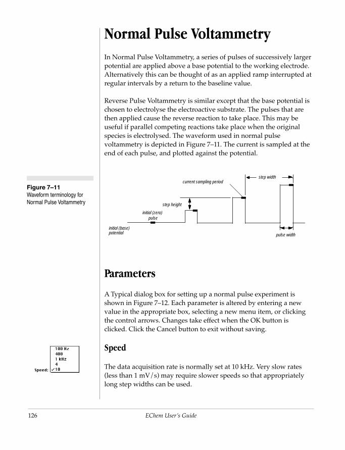
126
Figure 7–11 Waveform terminology for Normal Pulse Voltammetry
Normal Pulse VoltammetryIn Normal Pulse Voltammetry, a series of pulses of successively larger potential are applied above a base potential to the working electrode. Alternatively this can be thought of as an applied ramp interrupted at regular intervals by a return to the baseline value.
Reverse Pulse Voltammetry is similar except that the base potential is chosen to electrolyse the electroactive substrate. The pulses that are then applied cause the reverse reaction to take place. This may be useful if parallel competing reactions take place when the original species is electrolysed. The waveform used in normal pulse voltammetry is depicted in Figure 7–11. The current is sampled at the end of each pulse, and plotted against the potential.
Parameters
step width
step height
pulse width
current sampling period
initial (zero)pulse
initial (base)potential
EChem User’s Guide
A Typical dialog box for setting up a normal pulse experiment is shown in Figure 7–12. Each parameter is altered by entering a new value in the appropriate box, selecting a new menu item, or clicking the control arrows. Changes take effect when the OK button is clicked. Click the Cancel button to exit without saving.
Speed
The data acquisition rate is normally set at 10 kHz. Very slow rates (less than 1 mV/s) may require slower speeds so that appropriately long step widths can be used.

Chapter 7 — EChem Techn
Figure 7–12 The Normal Pulse Voltammetry dialog box
Range
The range pop-up menu selects the full scale range of the applied potential. Three ranges are available, ±1000 mV giving 0.5 mV resolution, ±2000 mV giving 1 mV resolution, or ±5000 mV giving 2.5 mV resolution, Table 7–1. Usually the 2000 mV range is chosen.
Initial (Potential)
This is the initial or starting potential of the ramp. This can be chosen between ± 2000 mV if on the 2000 mV range or ± 5000 mV when on the 5000 mV range. This value is usually chosen to be a value at which the electrode reaction of interest does not occur (so that the current is close to zero). For Reverse Pulse Voltammetry this potential is chosen to cause complete oxidation (or reduction) of the substrate, and the pulses then cause the reverse reaction.
Final (Potential)
iques 127
The potential voltage at which the ramp waveform finishes. This can be set between ± 2000 mV if on the 2000mV range or ± 5000 mV when on the 5000 mV range. The final potential may be either more negative than the initial potential (negative scan) or more positive than the initial potential (positive scan). This is the height of the last pulse to be applied. It can be thought of as the height of an imaginary ramp passing through the tops of the pulses.
(Scan) Rate
This sets the rate at which the ramp will be generated in mV per second. This is usually set between 5 and 100 mV s-1 for macro
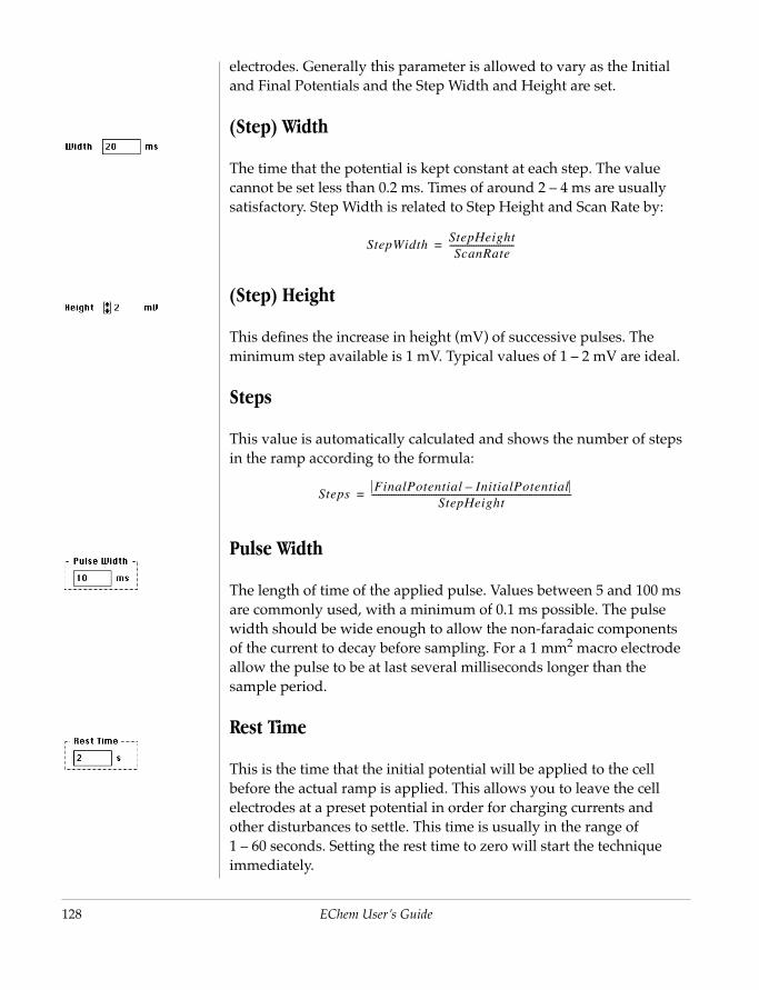
128
electrodes. Generally this parameter is allowed to vary as the Initial and Final Potentials and the Step Width and Height are set.
(Step) Width
The time that the potential is kept constant at each step. The value cannot be set less than 0.2 ms. Times of around 2 – 4 ms are usually satisfactory. Step Width is related to Step Height and Scan Rate by:
(Step) Height
This defines the increase in height (mV) of successive pulses. The minimum step available is 1 mV. Typical values of 1 – 2 mV are ideal.
Steps
This value is automatically calculated and shows the number of steps in the ramp according to the formula:
Pulse Width
The length of time of the applied pulse. Values between 5 and 100 ms are commonly used, with a minimum of 0.1 ms possible. The pulse width should be wide enough to allow the non-faradaic components
StepWidthStepHeightScanRate
-----------------------------=
StepsFinalPotential InitialPotential–
StepHeight------------------------------------------------------------------------------------------=
EChem User’s Guide
of the current to decay before sampling. For a 1 mm2 macro electrode allow the pulse to be at last several milliseconds longer than the sample period.
Rest Time
This is the time that the initial potential will be applied to the cell before the actual ramp is applied. This allows you to leave the cell electrodes at a preset potential in order for charging currents and other disturbances to settle. This time is usually in the range of 1 – 60 seconds. Setting the rest time to zero will start the technique immediately.
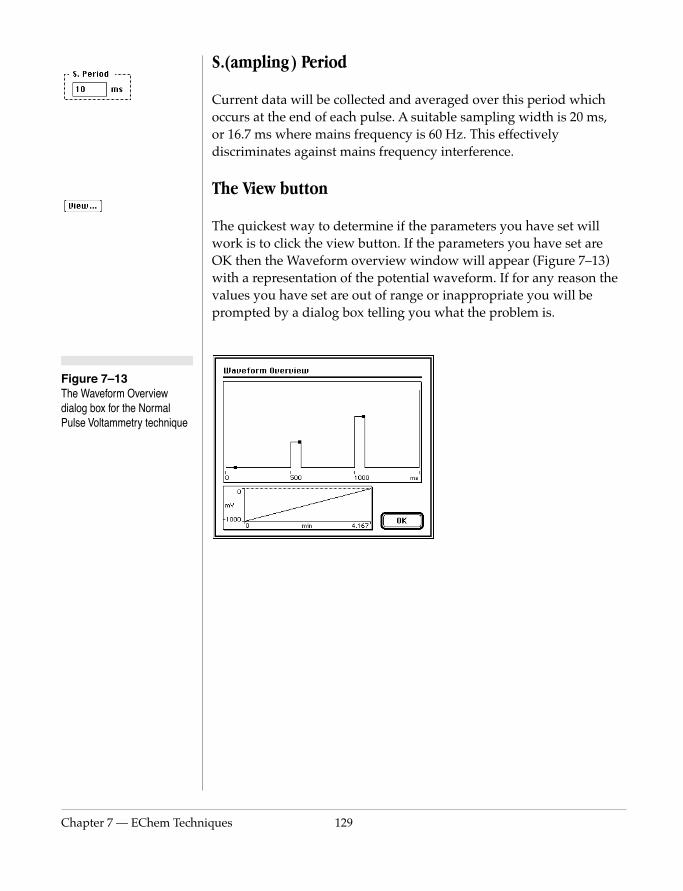
Chapter 7 — EChem Techn
Figure 7–13 The Waveform Overview dialog box for the Normal Pulse Voltammetry technique
S.(ampling) Period
Current data will be collected and averaged over this period which occurs at the end of each pulse. A suitable sampling width is 20 ms, or 16.7 ms where mains frequency is 60 Hz. This effectively discriminates against mains frequency interference.
The View button
The quickest way to determine if the parameters you have set will work is to click the view button. If the parameters you have set are OK then the Waveform overview window will appear (Figure 7–13) with a representation of the potential waveform. If for any reason the values you have set are out of range or inappropriate you will be prompted by a dialog box telling you what the problem is.
iques 129
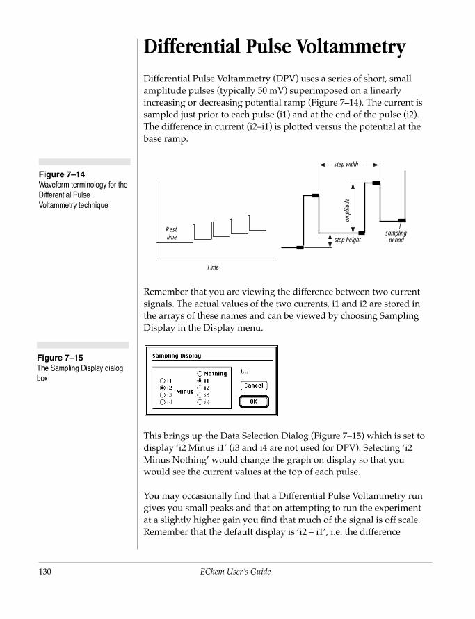
130
Figure 7–15 The Sampling Display dialog box
Differential Pulse VoltammetryDifferential Pulse Voltammetry (DPV) uses a series of short, small amplitude pulses (typically 50 mV) superimposed on a linearly increasing or decreasing potential ramp (Figure 7–14). The current is sampled just prior to each pulse (i1) and at the end of the pulse (i2). The difference in current (i2–i1) is plotted versus the potential at the base ramp.
Remember that you are viewing the difference between two current signals. The actual values of the two currents, i1 and i2 are stored in the arrays of these names and can be viewed by choosing Sampling Display in the Display menu.
Time
Resttime
step width
step heightsampling
ampl
itude
period
Figure 7–14 Waveform terminology for the Differential Pulse Voltammetry technique
EChem User’s Guide
This brings up the Data Selection Dialog (Figure 7–15) which is set to display ‘i2 Minus i1’ (i3 and i4 are not used for DPV). Selecting ‘i2 Minus Nothing’ would change the graph on display so that you would see the current values at the top of each pulse.
You may occasionally find that a Differential Pulse Voltammetry run gives you small peaks and that on attempting to run the experiment at a slightly higher gain you find that much of the signal is off scale. Remember that the default display is ‘i2 – i1’, i.e. the difference
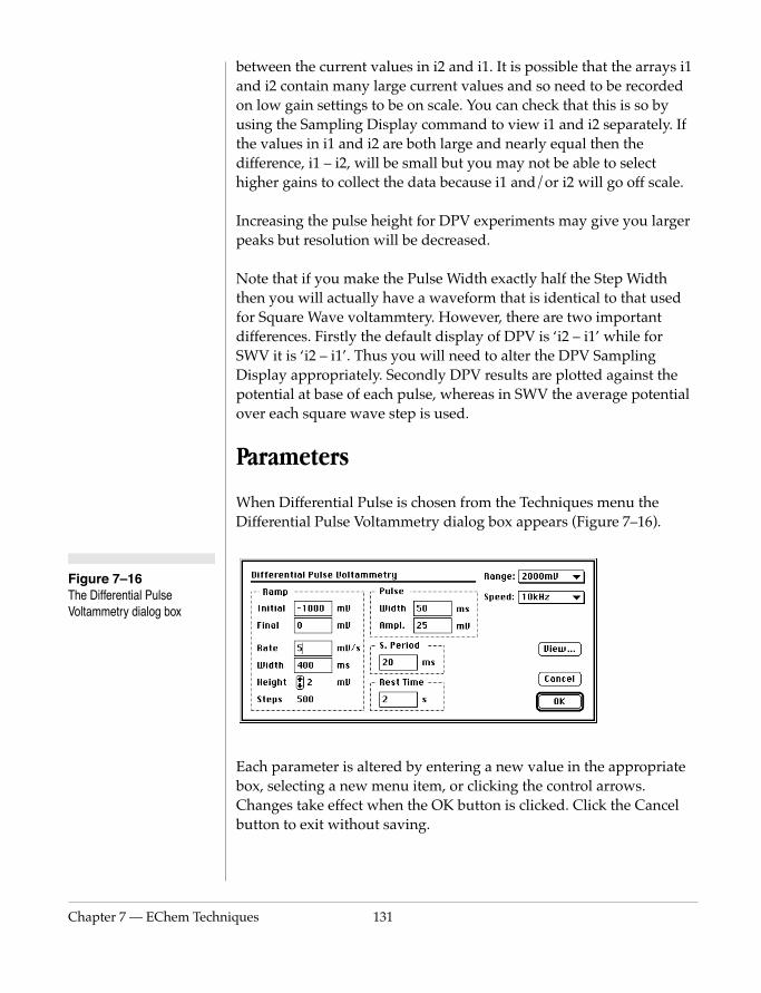
Chapter 7 — EChem Techn
Figure 7–16 The Differential Pulse Voltammetry dialog box
between the current values in i2 and i1. It is possible that the arrays i1 and i2 contain many large current values and so need to be recorded on low gain settings to be on scale. You can check that this is so by using the Sampling Display command to view i1 and i2 separately. If the values in i1 and i2 are both large and nearly equal then the difference, i1 – i2, will be small but you may not be able to select higher gains to collect the data because i1 and/or i2 will go off scale.
Increasing the pulse height for DPV experiments may give you larger peaks but resolution will be decreased.
Note that if you make the Pulse Width exactly half the Step Width then you will actually have a waveform that is identical to that used for Square Wave voltammtery. However, there are two important differences. Firstly the default display of DPV is ‘i2 – i1’ while for SWV it is ‘i2 – i1’. Thus you will need to alter the DPV Sampling Display appropriately. Secondly DPV results are plotted against the potential at base of each pulse, whereas in SWV the average potential over each square wave step is used.
Parameters
When Differential Pulse is chosen from the Techniques menu the Differential Pulse Voltammetry dialog box appears (Figure 7–16).
iques 131
Each parameter is altered by entering a new value in the appropriate box, selecting a new menu item, or clicking the control arrows. Changes take effect when the OK button is clicked. Click the Cancel button to exit without saving.
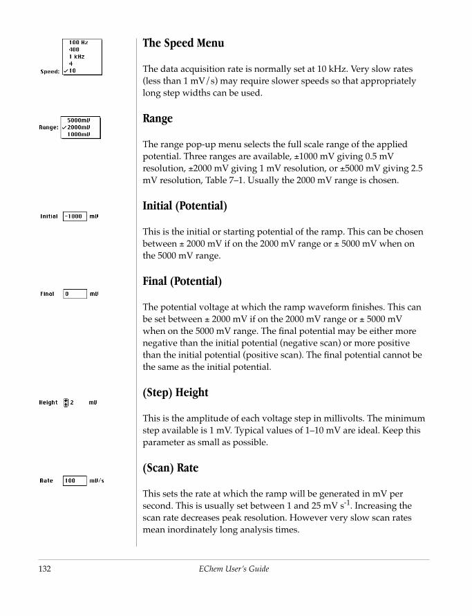
132
The Speed Menu
The data acquisition rate is normally set at 10 kHz. Very slow rates (less than 1 mV/s) may require slower speeds so that appropriately long step widths can be used.
Range
The range pop-up menu selects the full scale range of the applied potential. Three ranges are available, ±1000 mV giving 0.5 mV resolution, ±2000 mV giving 1 mV resolution, or ±5000 mV giving 2.5 mV resolution, Table 7–1. Usually the 2000 mV range is chosen.
Initial (Potential)
This is the initial or starting potential of the ramp. This can be chosen between ± 2000 mV if on the 2000 mV range or ± 5000 mV when on the 5000 mV range.
Final (Potential)
The potential voltage at which the ramp waveform finishes. This can be set between ± 2000 mV if on the 2000 mV range or ± 5000 mV when on the 5000 mV range. The final potential may be either more negative than the initial potential (negative scan) or more positive than the initial potential (positive scan). The final potential cannot be the same as the initial potential.
(Step) Height
EChem User’s Guide
This is the amplitude of each voltage step in millivolts. The minimum step available is 1 mV. Typical values of 1–10 mV are ideal. Keep this parameter as small as possible.
(Scan) Rate
This sets the rate at which the ramp will be generated in mV per second. This is usually set between 1 and 25 mV s-1. Increasing the scan rate decreases peak resolution. However very slow scan rates mean inordinately long analysis times.
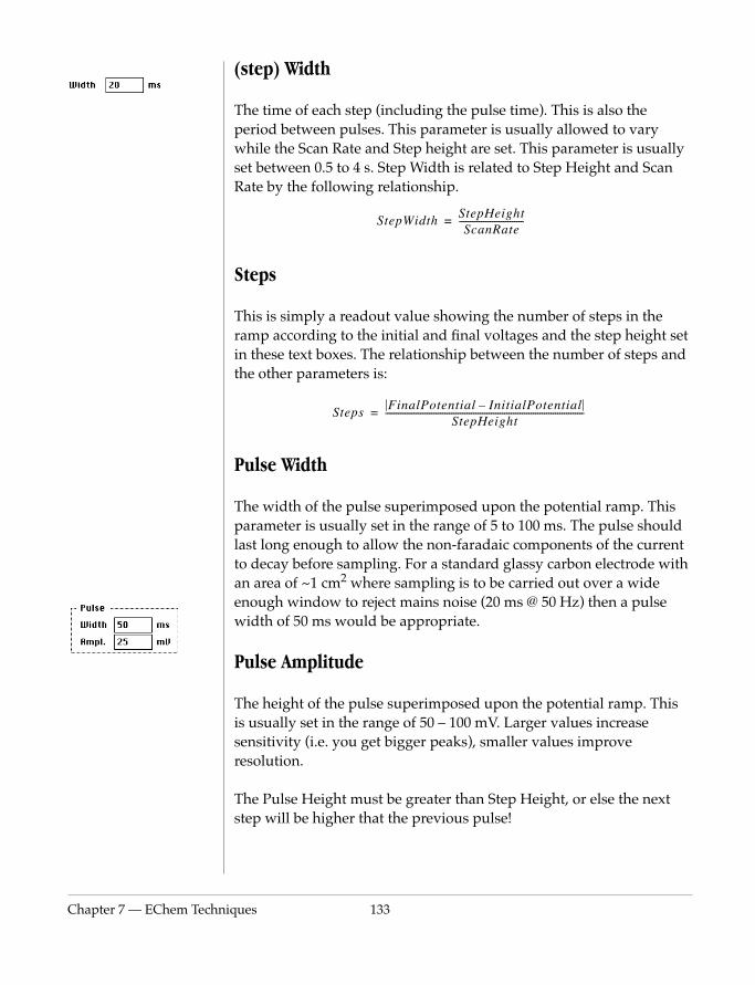
Chapter 7 — EChem Techn
(step) Width
The time of each step (including the pulse time). This is also the period between pulses. This parameter is usually allowed to vary while the Scan Rate and Step height are set. This parameter is usually set between 0.5 to 4 s. Step Width is related to Step Height and Scan Rate by the following relationship.
Steps
This is simply a readout value showing the number of steps in the ramp according to the initial and final voltages and the step height set in these text boxes. The relationship between the number of steps and the other parameters is:
Pulse Width
The width of the pulse superimposed upon the potential ramp. This parameter is usually set in the range of 5 to 100 ms. The pulse should last long enough to allow the non-faradaic components of the current to decay before sampling. For a standard glassy carbon electrode with an area of ~1 cm2 where sampling is to be carried out over a wide enough window to reject mains noise (20 ms @ 50 Hz) then a pulse width of 50 ms would be appropriate.
StepWidthStepHeightScanRate
-----------------------------=
StepsFinalPotential InitialPotential–
StepHeight------------------------------------------------------------------------------------------=
iques 133
Pulse Amplitude
The height of the pulse superimposed upon the potential ramp. This is usually set in the range of 50 – 100 mV. Larger values increase sensitivity (i.e. you get bigger peaks), smaller values improve resolution.
The Pulse Height must be greater than Step Height, or else the next step will be higher that the previous pulse!
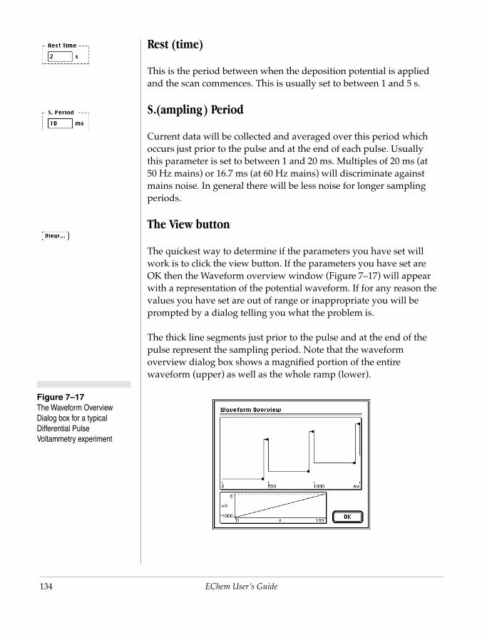
134
Figure 7–17 The Waveform Overview Dialog box for a typical Differential Pulse Voltammetry experiment
Rest (time)
This is the period between when the deposition potential is applied and the scan commences. This is usually set to between 1 and 5 s.
S.(ampling) Period
Current data will be collected and averaged over this period which occurs just prior to the pulse and at the end of each pulse. Usually this parameter is set to between 1 and 20 ms. Multiples of 20 ms (at 50 Hz mains) or 16.7 ms (at 60 Hz mains) will discriminate against mains noise. In general there will be less noise for longer sampling periods.
The View button
The quickest way to determine if the parameters you have set will work is to click the view button. If the parameters you have set are OK then the Waveform overview window (Figure 7–17) will appear with a representation of the potential waveform. If for any reason the values you have set are out of range or inappropriate you will be prompted by a dialog telling you what the problem is.
The thick line segments just prior to the pulse and at the end of the pulse represent the sampling period. Note that the waveform overview dialog box shows a magnified portion of the entire waveform (upper) as well as the whole ramp (lower).
EChem User’s Guide

Chapter 7 — EChem Techn
Stripping TechniquesEChem allows you to perform stripping type techniques using any one of the five standard methods just described. EChem supports;
• Linear sweep stripping voltammetry• Differential pulse stripping voltammetry• Square wave stripping voltammetry• Normal pulse stripping voltammetry
In addition non-standard stripping experiments can also be set up in the Cyclic and MultiPulse Techniques. Stripping techniques involve fixing the analyte to the working electrode in some way. This has the advantage of concentrating the analyte at the electrode and giving a dramatic increase in sensitivity.
The two main methods in this area are cathodic stripping voltammetry and anodic stripping voltammetry. Both methods make use of a constant deposition potential applied prior to beginning of the experiment proper. Similarly after the experiment a constant cleaning potential can be maintained for a fixed time period.
Anodic Stripping Voltammetry
Anodic stripping techniques usually involve the use of mercury as a working electrode. This may be in the form a hanging mercury drop electrode (HMDE), or a mercury film electrode (MFE). The function of the mercury is to amalgamate with (dissolve) metals that plate out on
iques 135
the electrode surface when metal ions in solution are reduced. Solid electrodes can also be used but mercury usually gives superior performance.
Prior to the experiment a reduction step takes place when a deposition potential is applied to the mercury working electrode. This potential is maintained, usually while stirring the solution, so that the metal ions of interest in the sample are concentrated within the mercury electrode. The deposition potential should be at least 0.2 V more reducing than the peak potential of the most electropositive metal to be detected.
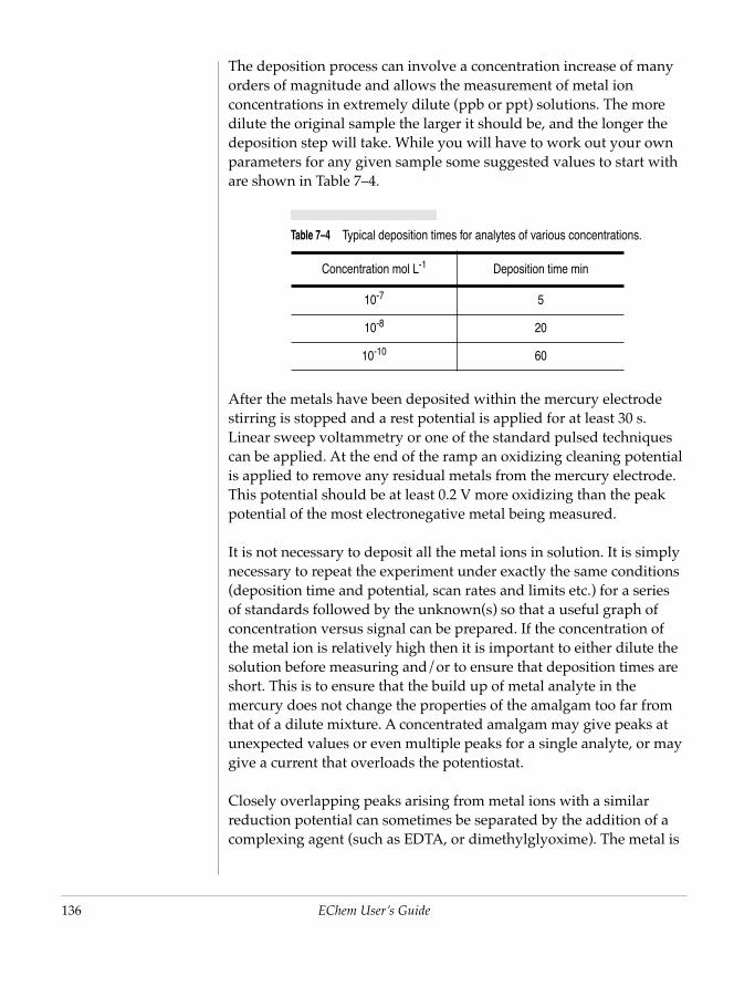
136
The deposition process can involve a concentration increase of many orders of magnitude and allows the measurement of metal ion concentrations in extremely dilute (ppb or ppt) solutions. The more dilute the original sample the larger it should be, and the longer the deposition step will take. While you will have to work out your own parameters for any given sample some suggested values to start with are shown in Table 7–4.
After the metals have been deposited within the mercury electrode stirring is stopped and a rest potential is applied for at least 30 s. Linear sweep voltammetry or one of the standard pulsed techniques can be applied. At the end of the ramp an oxidizing cleaning potential is applied to remove any residual metals from the mercury electrode. This potential should be at least 0.2 V more oxidizing than the peak potential of the most electronegative metal being measured.
It is not necessary to deposit all the metal ions in solution. It is simply necessary to repeat the experiment under exactly the same conditions (deposition time and potential, scan rates and limits etc.) for a series of standards followed by the unknown(s) so that a useful graph of concentration versus signal can be prepared. If the concentration of
Table 7–4 Typical deposition times for analytes of various concentrations.
Concentration mol L-1 Deposition time min
10-7 5
10-8 20
10-10 60
EChem User’s Guide
the metal ion is relatively high then it is important to either dilute the solution before measuring and/or to ensure that deposition times are short. This is to ensure that the build up of metal analyte in the mercury does not change the properties of the amalgam too far from that of a dilute mixture. A concentrated amalgam may give peaks at unexpected values or even multiple peaks for a single analyte, or may give a current that overloads the potentiostat.
Closely overlapping peaks arising from metal ions with a similar reduction potential can sometimes be separated by the addition of a complexing agent (such as EDTA, or dimethylglyoxime). The metal is

Chapter 7 — EChem Techn
then no longer present in solution as an aquated metal ion but as a complex ion with a different reduction potential.
Cathodic Stripping Voltammetry
Anions can be fixed to an electrode as an insoluble metal salt. In the case of analyzing for halides an oxidizing deposition potential is first applied at a silver electrode:
Ag(s) + I-(aq) → AgI(s) + e-
A subsequent scan to reducing potential can be used to detect the halide(s) present as the silver halide is reduced:
AgI(s) + e- → Ag(s) + I-(aq)
Other anions that can be detected include sulfide, phosphate, arsenate, and arsenite. The working electrode is usually made of mercury, gold or silver.
Setting Parameters
When any of the stripping techniques are chosen from the Technique menu, a dialog box will appear (Figure 7–18). The dialog is similar to the non-stripping technique dialog except that extra controls for Deposition and Cleaning appear at the bottom of the dialog box. You can set a potential, and a time period, for both deposition and cleaning. All the Stripping techniques carry out deposition first, followed by the actual technique and then cleaning takes place.
iques 137
Both the deposition and Clean Time periods can be turned off using the check boxes next to their titles. By tuning off both the Deposition and Clean Time periods then only the basic technique will be left. For example, when using Cyclic Voltammetry you should leave both check boxes off unless you are attempting an unconventional experiment.
The ramp and pulse parameters are set up in the same way as for the corresponding non-stripping technique. Refer to the corresponding non-stripping technique for information on these parameters.
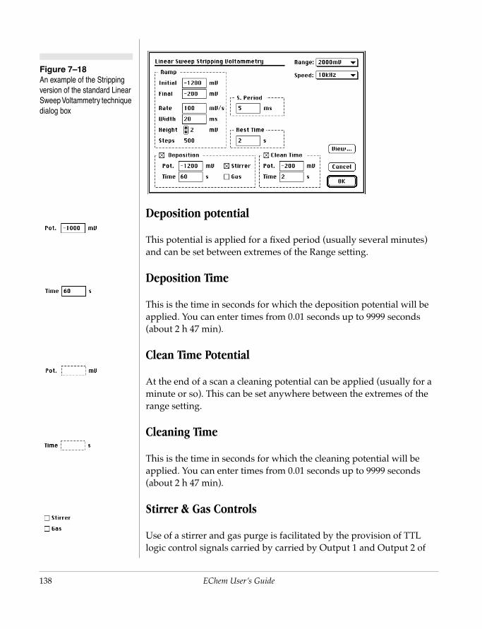
138
Figure 7–18 An example of the Stripping version of the standard Linear Sweep Voltammetry technique dialog box
Deposition potential
This potential is applied for a fixed period (usually several minutes) and can be set between extremes of the Range setting.
Deposition Time
This is the time in seconds for which the deposition potential will be applied. You can enter times from 0.01 seconds up to 9999 seconds (about 2 h 47 min).
Clean Time Potential
At the end of a scan a cleaning potential can be applied (usually for a minute or so). This can be set anywhere between the extremes of the
EChem User’s Guide
range setting.
Cleaning Time
This is the time in seconds for which the cleaning potential will be applied. You can enter times from 0.01 seconds up to 9999 seconds (about 2 h 47 min).
Stirrer & Gas Controls
Use of a stirrer and gas purge is facilitated by the provision of TTL logic control signals carried by carried by Output 1 and Output 2 of
Chapter 7 — EChem Techn
TTL logic signals are a simple means of on/off communication between instruments. ‘TTL high’ corresponds to a voltage level of about 5 V, while ‘TTL low’ corresponds to a signal of about 0 V. These states are controlled in software by a single bit variable which is referred to as being set on or off.
CAUTION. Connection of the PowerLab to an external stirrer and purge system should only be attempted by a qualified electronics technician.
the PowerLab digital output, page 160. The Stirrer check box controls digital output 1 and the Gas check box controls digital output 2 of the PowerLab. Refer to your PowerLab Owners Guide for details of the digital output signals and how to connect to them. Note that on PowerLab/200 /400 and the older /2e and /4e units the digital output signals are provided on the Multiport connector on the rear of the unit. Other PowerLab models have a dedicated digital output connector. The digital I/O ports provide 0 – 5 V at about 1 mA. This is enough to act as an on/off signal but is not sufficient to power a stirrer or other equipment.
Checking the Gas and/or Stirrer checkboxes allows you to control the state of an external stirrer motor or solenoid gas valve during deposition. These check boxes control two of the digital output (TTL) lines provided by the PowerLab. Activating these controls (click the check box) will set the corresponding digital output on at appropriate times during the experiment. Output 1 is on during the Deposition and Cleaning periods, while Output 2 is on during the Deposition time only. A cable can be made to use these signals to turn a stirrer and solenoid gas valve on and off during the stripping experiment.
You can monitor the state of the digital output lines by displaying the Digital Output panel, Figure 7–32.
iques 139
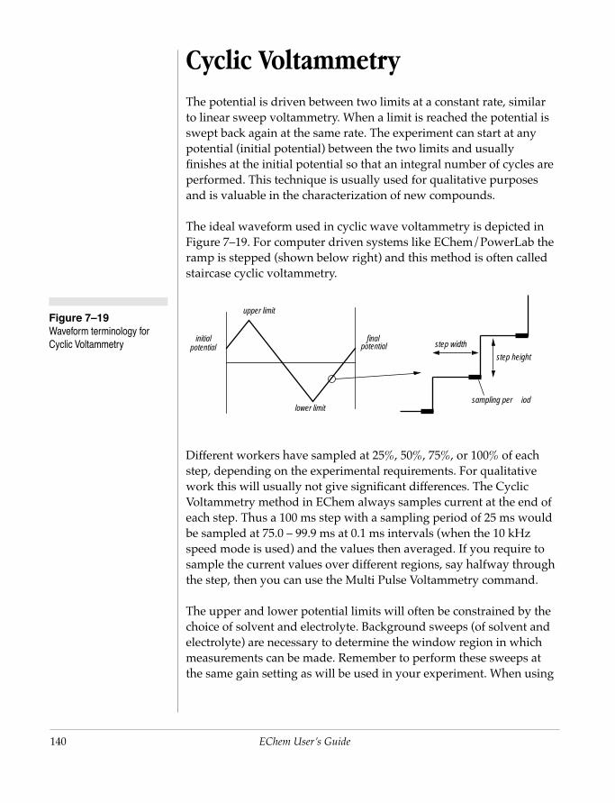
140
Figure 7–19 Waveform terminology for Cyclic Voltammetry
Cyclic VoltammetryThe potential is driven between two limits at a constant rate, similar to linear sweep voltammetry. When a limit is reached the potential is swept back again at the same rate. The experiment can start at any potential (initial potential) between the two limits and usually finishes at the initial potential so that an integral number of cycles are performed. This technique is usually used for qualitative purposes and is valuable in the characterization of new compounds.
The ideal waveform used in cyclic wave voltammetry is depicted in Figure 7–19. For computer driven systems like EChem/PowerLab the ramp is stepped (shown below right) and this method is often called staircase cyclic voltammetry.
Different workers have sampled at 25%, 50%, 75%, or 100% of each step, depending on the experimental requirements. For qualitative work this will usually not give significant differences. The Cyclic Voltammetry method in EChem always samples current at the end of
step width
step height
sampling per iod
initial
upper limit
lower limit
final potential potential
EChem User’s Guide
each step. Thus a 100 ms step with a sampling period of 25 ms would be sampled at 75.0 – 99.9 ms at 0.1 ms intervals (when the 10 kHz speed mode is used) and the values then averaged. If you require to sample the current values over different regions, say halfway through the step, then you can use the Multi Pulse Voltammetry command.
The upper and lower potential limits will often be constrained by the choice of solvent and electrolyte. Background sweeps (of solvent and electrolyte) are necessary to determine the window region in which measurements can be made. Remember to perform these sweeps at the same gain setting as will be used in your experiment. When using
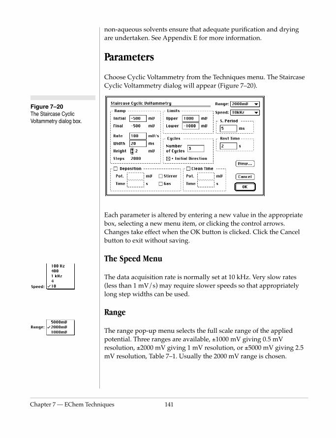
Chapter 7 — EChem Techn
Figure 7–20 The Staircase Cyclic Voltammetry dialog box.
non-aqueous solvents ensure that adequate purification and drying are undertaken. See Appendix E for more information.
Parameters
Choose Cyclic Voltammetry from the Techniques menu. The Staircase Cyclic Voltammetry dialog will appear (Figure 7–20).
Each parameter is altered by entering a new value in the appropriate box, selecting a new menu item, or clicking the control arrows. Changes take effect when the OK button is clicked. Click the Cancel button to exit without saving.
The Speed Menu
The data acquisition rate is normally set at 10 kHz. Very slow rates
iques 141
(less than 1 mV/s) may require slower speeds so that appropriately long step widths can be used.
Range
The range pop-up menu selects the full scale range of the applied potential. Three ranges are available, ±1000 mV giving 0.5 mV resolution, ±2000 mV giving 1 mV resolution, or ±5000 mV giving 2.5 mV resolution, Table 7–1. Usually the 2000 mV range is chosen.
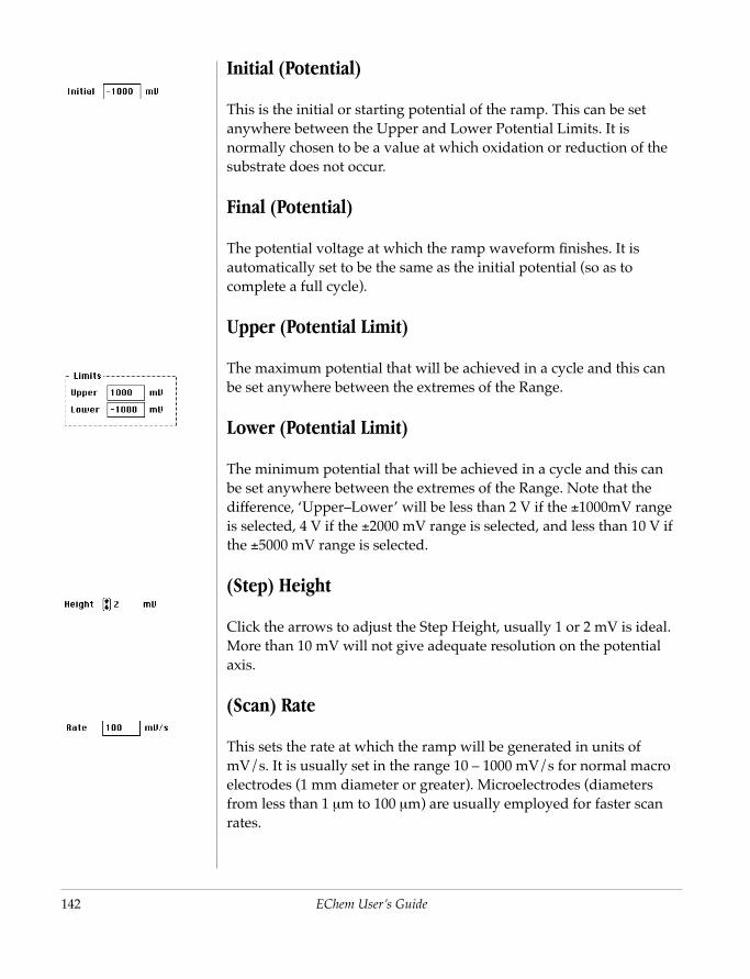
142
Initial (Potential)
This is the initial or starting potential of the ramp. This can be set anywhere between the Upper and Lower Potential Limits. It is normally chosen to be a value at which oxidation or reduction of the substrate does not occur.
Final (Potential)
The potential voltage at which the ramp waveform finishes. It is automatically set to be the same as the initial potential (so as to complete a full cycle).
Upper (Potential Limit)
The maximum potential that will be achieved in a cycle and this can be set anywhere between the extremes of the Range.
Lower (Potential Limit)
The minimum potential that will be achieved in a cycle and this can be set anywhere between the extremes of the Range. Note that the difference, ‘Upper–Lower’ will be less than 2 V if the ±1000mV range is selected, 4 V if the ±2000 mV range is selected, and less than 10 V if the ±5000 mV range is selected.
(Step) Height
EChem User’s Guide
Click the arrows to adjust the Step Height, usually 1 or 2 mV is ideal. More than 10 mV will not give adequate resolution on the potential axis.
(Scan) Rate
This sets the rate at which the ramp will be generated in units of mV/s. It is usually set in the range 10 – 1000 mV/s for normal macro electrodes (1 mm diameter or greater). Microelectrodes (diameters from less than 1 µm to 100 µm) are usually employed for faster scan rates.
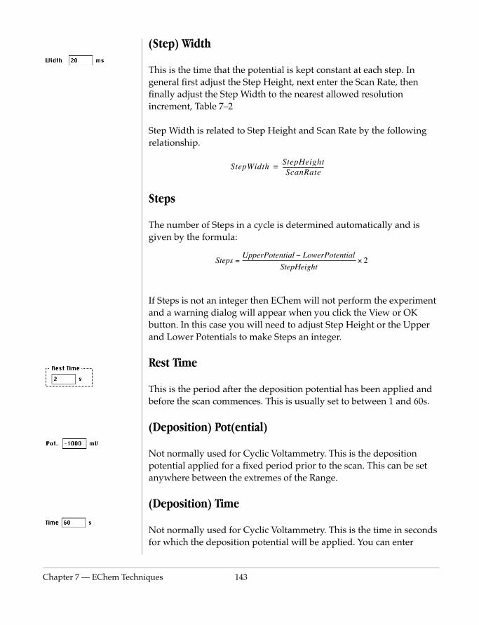
Chapter 7 — EChem Techn
(Step) Width
This is the time that the potential is kept constant at each step. In general first adjust the Step Height, next enter the Scan Rate, then finally adjust the Step Width to the nearest allowed resolution increment, Table 7–2
Step Width is related to Step Height and Scan Rate by the following relationship.
Steps
The number of Steps in a cycle is determined automatically and is given by the formula:
If Steps is not an integer then EChem will not perform the experiment and a warning dialog will appear when you click the View or OK button. In this case you will need to adjust Step Height or the Upper and Lower Potentials to make Steps an integer.
Rest Time
This is the period after the deposition potential has been applied and
StepWidthStepHeightScanRate
-----------------------------=
Steps =UpperPotential − LowerPotential
StepHeight× 2
iques 143
before the scan commences. This is usually set to between 1 and 60s.
(Deposition) Pot(ential)
Not normally used for Cyclic Voltammetry. This is the deposition potential applied for a fixed period prior to the scan. This can be set anywhere between the extremes of the Range.
(Deposition) Time
Not normally used for Cyclic Voltammetry. This is the time in seconds for which the deposition potential will be applied. You can enter
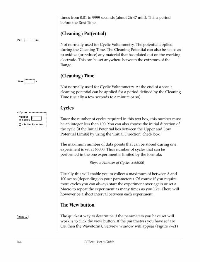
144
times from 0.01 to 9999 seconds (about 2h 47 min). This a period before the Rest Time.
(Cleaning) Pot(ential)
Not normally used for Cyclic Voltammetry. The potential applied during the Cleaning Time. The Cleaning Potential can also be set so as to oxidize (or reduce) any material that has plated out on the working electrode. This can be set anywhere between the extremes of the Range.
(Cleaning) Time
Not normally used for Cyclic Voltammetry. At the end of a scan a cleaning potential can be applied for a period defined by the Cleaning Time (usually a few seconds to a minute or so).
Cycles
Enter the number of cycles required in this text box, this number must be an integer less than 100. You can also choose the initial direction of the cycle (if the Initial Potential lies between the Upper and Low Potential Limits) by using the ‘Initial Direction’ check box.
The maximum number of data points that can be stored during one experiment is set at 65000. Thus number of cycles that can be performed in the one experiment is limited by the formula:
Steps × Number of Cycles ≤ 65000
EChem User’s Guide
Usually this will enable you to collect a maximum of between 8 and 100 scans (depending on your parameters). Of course if you require more cycles you can always start the experiment over again or set a Macro to repeat the experiment as many times as you like. There will however be a short interval between each experiment.
The View button
The quickest way to determine if the parameters you have set will work is to click the view button. If the parameters you have set are OK then the Waveform Overview window will appear (Figure 7–21)
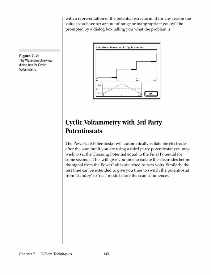
Chapter 7 — EChem Techn
Figure 7–21 The Waveform Overview dialog box for Cyclic Voltammetry.
with a representation of the potential waveform. If for any reason the values you have set are out of range or inappropriate you will be prompted by a dialog box telling you what the problem is:
Cyclic Voltammetry with 3rd Party Potentiostats
The PowerLab Potentiostat will automatically isolate the electrodes after the scan but if you are using a third party potentiostat you may wish to set the Cleaning Potential equal to the Final Potential for some seconds. This will give you time to isolate the electrodes before the signal from the PowerLab is switched to zero volts. Similarly the rest time can be extended to give you time to switch the potentiostat from ‘standby’ to ‘real’ mode before the scan commences.
iques 145

146
MultiPulse VoltammetryThe MultiPulse Voltammetry technique allows you to generate your own waveform. This is constructed by the addition of a staircase ramp and one or two pulses per step of the ramp. These pulses may be either positive or negative and may be increased or decreased throughout the scan. Using this dialog the operator is able to define any one of a number of regularly used techniques. There is also the added flexibility of being able to define an unusual pulse sequence. In addition up to four current sampling windows can be selected with their position and duration independently set.
A library of different signals, that can be used at any time, can be achieved by writing Macros that include the Multi Pulse method or by storing MultiPulse parameters in Settings files. This will allow you to automate your experiments.
Note that if you want to set up a non-standard or cyclic Square Wave voltammetry experiment then you will need to make the Pulse Width exactly half the Step Width. Remember to adjust the Sampling Display to i1-i2. Also MultiPulse Voltammetry results the default display is to plot current against the potential at the base of each pulse, whereas in the Square Wave Voltammetry technique the average potential over each step is used.
Parameters
To use the MultiPulse technique, select the Multi Pulse method from
EChem User’s Guide
the Techniques menu. The MultiPulse dialog will appear (Figure 7–22).
Each parameter is altered by entering a new value in the appropriate box, selecting a new menu item, or clicking the control arrows. Changes take effect when the OK button is clicked. Click the Cancel button to exit without saving.
Ramp parameters
First the Ramp parameters are adjusted. These have a similar function to the parameters used for linear sweep voltammetry.
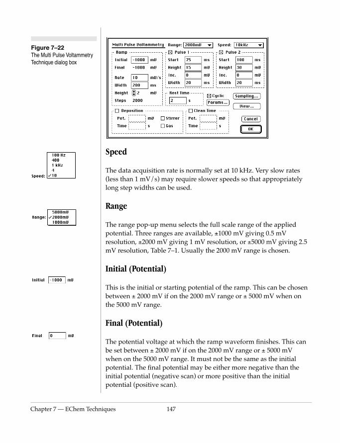
Chapter 7 — EChem Techn
Figure 7–22 The Multi Pulse Voltammetry Technique dialog box
Speed
The data acquisition rate is normally set at 10 kHz. Very slow rates (less than 1 mV/s) may require slower speeds so that appropriately long step widths can be used.
Range
The range pop-up menu selects the full scale range of the applied potential. Three ranges are available, ±1000 mV giving 0.5 mV resolution, ±2000 mV giving 1 mV resolution, or ±5000 mV giving 2.5 mV resolution, Table 7–1. Usually the 2000 mV range is chosen.
Initial (Potential)
iques 147
This is the initial or starting potential of the ramp. This can be chosen between ± 2000 mV if on the 2000 mV range or ± 5000 mV when on the 5000 mV range.
Final (Potential)
The potential voltage at which the ramp waveform finishes. This can be set between ± 2000 mV if on the 2000 mV range or ± 5000 mV when on the 5000 mV range. It must not be the same as the initial potential. The final potential may be either more negative than the initial potential (negative scan) or more positive than the initial potential (positive scan).
148
(Scan) Rate
This sets the rate at which the ramp will be generated in mV per second. It is usually set less than 1 mV s-1 for corrosion work or in the range of 5 to 1000 mV s-1 for other work. Faster scan rates lead to a higher background signal.
(Step) Width
The time that the potential is kept constant at each step. Step Width is related to Step Height and Scan Rate by:
(Step) Height
The size of each step. The value of this parameter will depend on the experiment being performed. But it is usually less than 10 mV.
Steps
This is simply a readout value showing the number of steps in the ramp according to the initial and final voltages and the step height set in these text boxes. The relationship between the number of steps and the other parameters is:
StepWidthStepHeightScanRate
-----------------------------=
StepsFinalPotential InitialPotential–
StepHeight------------------------------------------------------------------------------------------=
EChem User’s Guide
Rest Time
This is the period between when the deposition potential is applied and the scan commences. This is usually set to between 1 and 5 s, or longer for corrosion work.
Chapter 7 — EChem Techn
Figure 7–23 The Cyclic Parameters dialog box
Cyclic
Clicking the Cyclic checkbox will activate the Params... button. This also automatically sets the Final Potential equal to the Initial Potential (so that the cycle will be complete)
Params...
Clicking the Params... button brings up the Cyclic Parameters dialog box, Figure 7–23, so that a cyclic waveform can be set up. You can enter the Upper and Lower Limits of the scan, the Number of Cycles to be performed, and the Initial Direction of the scan (if the Initial Potential lies between the extremes of the Upper and Lower Potential. See the section on Cyclic Voltammetry for more information on the operation of these parameters.
Defining pulses
iques 149
For each step of the staircase ramp two pulses may be used. Each pulse is activated by clicking the box in the upper left-hand corner of the pulse panel, and now the relevant parameters can be entered.
(Pulse) Start
The timing of each pulse is linked to the start of each step in the base ramp. For example if you enter 20 ms in the Start box it means the pulse will be activated 20 ms after the beginning of the step. The pulse can begin at any time during each step and must be less than the Step Width. If you are using a PowerLab/200, /400, /800 or /2e, /4e or /8e then try to avoid starting pulses at 0 ms or starting two
150
pulses at the same time when constructing a waveform. There will be a short delay (a few microseconds) between the beginning of apparently concurrent events. Often a waveform of the same shape can be construct by placing the pulse towards the end of the step. The PowerLab/4s, /4SP, /8s and /16s do not suffer these limitations.
(Pulse) Height
The height of the pulse superimposed upon the potential ramp. Note that the value for the height of the pulse is added to the potential of the staircase ramp. If two pulses are made to overlap then the ramp and pulse potentials are all added together over this period.
Inc(rement)
Pulses on successive steps will be incremented by this amount.
Width
The duration of the pulse must be such that the entire pulse occurs within one step of the potential ramp.
This is best explained by examples. The dialog box shown in Figure 7–24 sets up two simple pulses, each 100 ms long, on each 500 ms step of the ramp. Clicking the View... button Waveform Overview window displays the appearance of several steps of the ramp, Figure 7–25.
EChem User’s Guide
The Sampling Dialog
By clicking the Sampling... button in the Multi Pulse dialog the Sampling Time dialog in Figure 7–26 is activated. This dialog box allows you to nominate the current sampling periods. This involves choosing the time and duration of each of up to 4 sampling periods (i1, i2, i3, and i4).
The dialog box is divided into four panels which control each of the four sampling periods available.
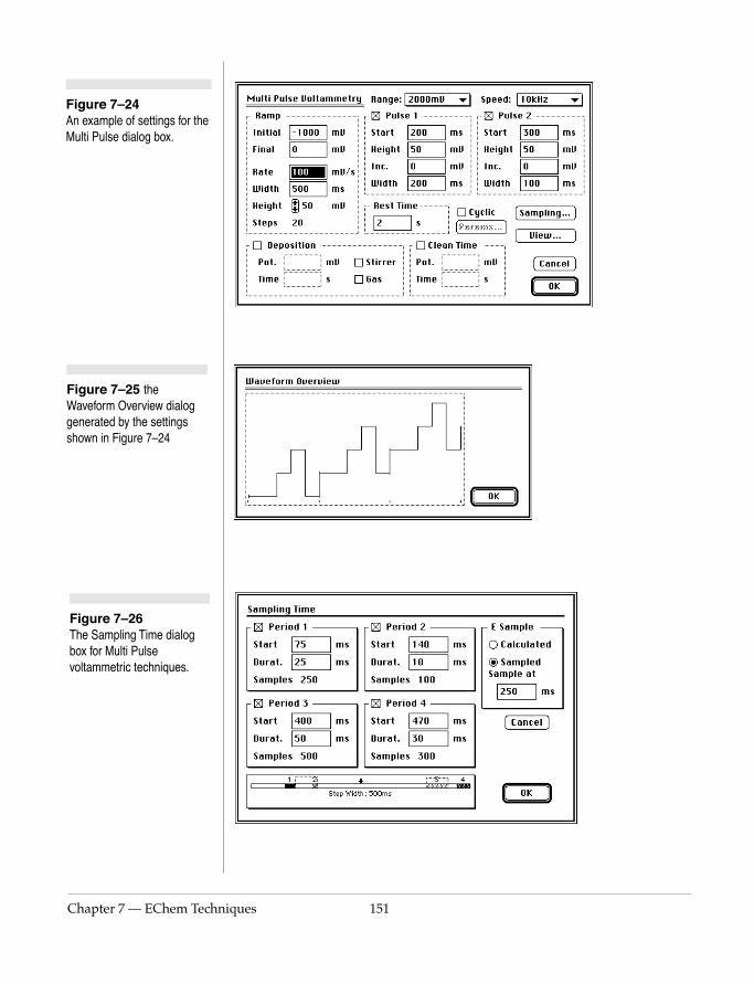
Chapter 7 — EChem Techn
Figure 7–26 The Sampling Time dialog box for Multi Pulse voltammetric techniques.
Figure 7–24 An example of settings for the Multi Pulse dialog box.
Figure 7–25 the Waveform Overview dialog generated by the settings shown in Figure 7–24
iques 151
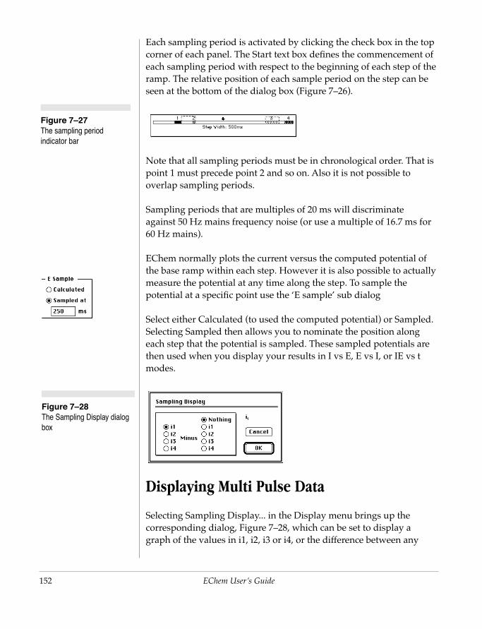
152
Figure 7–27 The sampling period indicator bar
Figure 7–28 The Sampling Display dialog box
Each sampling period is activated by clicking the check box in the top corner of each panel. The Start text box defines the commencement of each sampling period with respect to the beginning of each step of the ramp. The relative position of each sample period on the step can be seen at the bottom of the dialog box (Figure 7–26).
Note that all sampling periods must be in chronological order. That is point 1 must precede point 2 and so on. Also it is not possible to overlap sampling periods.
Sampling periods that are multiples of 20 ms will discriminate against 50 Hz mains frequency noise (or use a multiple of 16.7 ms for 60 Hz mains).
EChem normally plots the current versus the computed potential of the base ramp within each step. However it is also possible to actually measure the potential at any time along the step. To sample the potential at a specific point use the ‘E sample’ sub dialog
Select either Calculated (to used the computed potential) or Sampled. Selecting Sampled then allows you to nominate the position along each step that the potential is sampled. These sampled potentials are then used when you display your results in I vs E, E vs I, or IE vs t modes.
EChem User’s Guide
Displaying Multi Pulse Data
Selecting Sampling Display... in the Display menu brings up the corresponding dialog, Figure 7–28, which can be set to display a graph of the values in i1, i2, i3 or i4, or the difference between any

Chapter 7 — EChem Techn
two of these. If you require to display more complicated functions you will need to transfer the data to a spreadsheet or graphing application.
iques 153
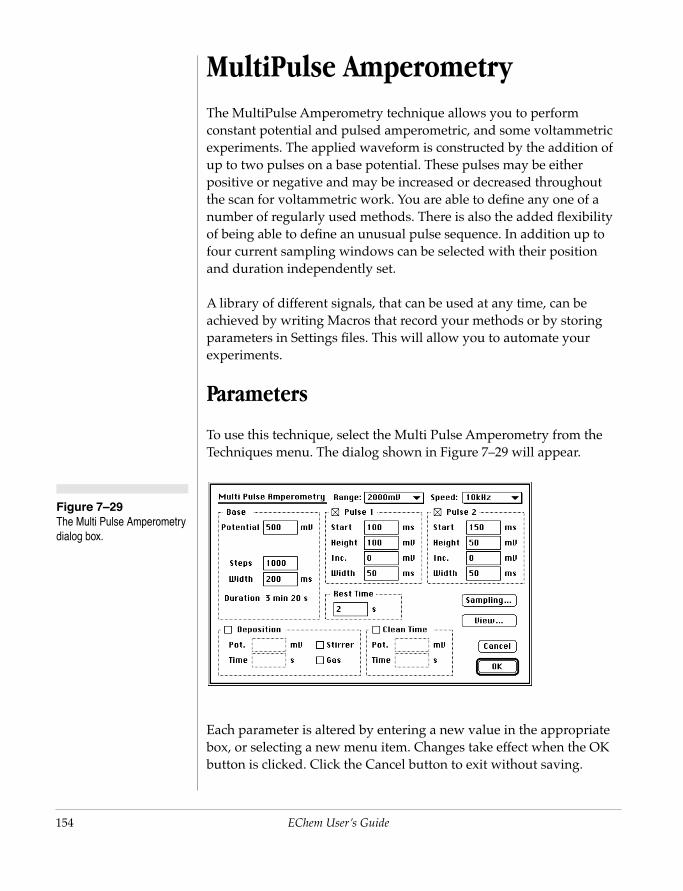
154
Figure 7–29 The Multi Pulse Amperometry dialog box.
MultiPulse AmperometryThe MultiPulse Amperometry technique allows you to perform constant potential and pulsed amperometric, and some voltammetric experiments. The applied waveform is constructed by the addition of up to two pulses on a base potential. These pulses may be either positive or negative and may be increased or decreased throughout the scan for voltammetric work. You are able to define any one of a number of regularly used methods. There is also the added flexibility of being able to define an unusual pulse sequence. In addition up to four current sampling windows can be selected with their position and duration independently set.
A library of different signals, that can be used at any time, can be achieved by writing Macros that record your methods or by storing parameters in Settings files. This will allow you to automate your experiments.
Parameters
To use this technique, select the Multi Pulse Amperometry from the Techniques menu. The dialog shown in Figure 7–29 will appear.
EChem User’s Guide
Each parameter is altered by entering a new value in the appropriate box, or selecting a new menu item. Changes take effect when the OK button is clicked. Click the Cancel button to exit without saving.
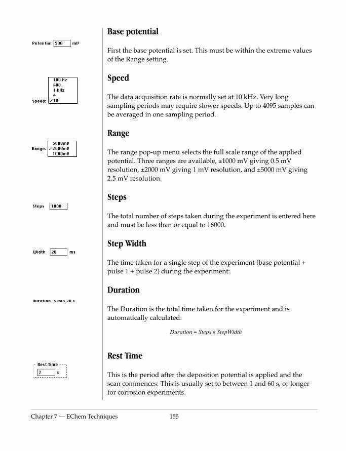
Chapter 7 — EChem Techn
Base potential
First the base potential is set. This must be within the extreme values of the Range setting.
Speed
The data acquisition rate is normally set at 10 kHz. Very long sampling periods may require slower speeds. Up to 4095 samples can be averaged in one sampling period.
Range
The range pop-up menu selects the full scale range of the applied potential. Three ranges are available, ±1000 mV giving 0.5 mV resolution, ±2000 mV giving 1 mV resolution, and ±5000 mV giving 2.5 mV resolution.
Steps
The total number of steps taken during the experiment is entered here and must be less than or equal to 16000.
Step Width
The time taken for a single step of the experiment (base potential + pulse 1 + pulse 2) during the experiment:
iques 155
Duration
The Duration is the total time taken for the experiment and is automatically calculated:
Rest Time
This is the period after the deposition potential is applied and the scan commences. This is usually set to between 1 and 60 s, or longer for corrosion experiments.
Duration = Steps × StepWidth

156
Defining pulses
For each step up to two pulses may be applied. Each pulse is activated by clicking the box in the upper left-hand corner of the pulse panel, and now the relevant parameters can be entered.
(Pulse) Start
The timing of each pulse is linked to the start of each step. For example if you enter 100 ms in the Start box it means the pulse will be activated 100 ms after the beginning of the step. The pulse can begin at any time during each step but the start time must be less than the Step Width
(Pulse) Height
The height of the pulse. Make sure that the sum of the base and pulse potentials does not exceed the Range setting.
Note that the value for the height of the pulse is added to the base potential. If two pulses are made to overlap then the base and two pulse potentials are all added together over this period.
Inc(rement)
Pulses on successive steps will be incremented by this amount. If you enter a non zero value you will probably be doing a pulsed voltammetric experiment ie the potential will be changing in a ramp-
EChem User’s Guide
like manner during the experiment.
Width
The duration of the pulse must be such that the entire pulse occurs within one step of the experiment.
This is best explained by examples. The dialog box shown in Figure 7–30 sets up two simple pulses, each 100 ms long, on each 500 ms step of the experiment.
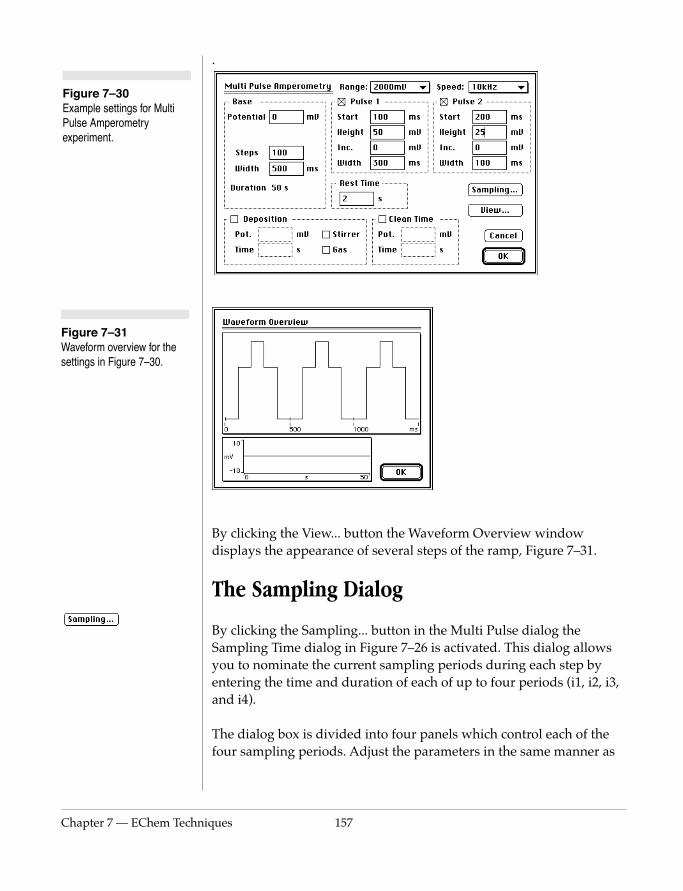
Chapter 7 — EChem Techn
Figure 7–31 Waveform overview for the settings in Figure 7–30.
.
By clicking the View... button the Waveform Overview window displays the appearance of several steps of the ramp, Figure 7–31.
Figure 7–30 Example settings for Multi Pulse Amperometry experiment.
iques 157
The Sampling Dialog
By clicking the Sampling... button in the Multi Pulse dialog the Sampling Time dialog in Figure 7–26 is activated. This dialog allows you to nominate the current sampling periods during each step by entering the time and duration of each of up to four periods (i1, i2, i3, and i4).
The dialog box is divided into four panels which control each of the four sampling periods. Adjust the parameters in the same manner as
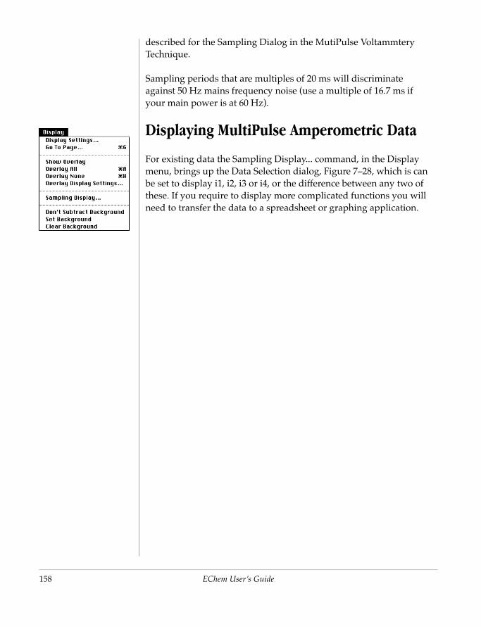
158
described for the Sampling Dialog in the MutiPulse Voltammtery Technique.
Sampling periods that are multiples of 20 ms will discriminate against 50 Hz mains frequency noise (use a multiple of 16.7 ms if your main power is at 60 Hz).
Displaying MultiPulse Amperometric Data
For existing data the Sampling Display... command, in the Display menu, brings up the Data Selection dialog, Figure 7–28, which is can be set to display i1, i2, i3 or i4, or the difference between any two of these. If you require to display more complicated functions you will need to transfer the data to a spreadsheet or graphing application.
EChem User’s Guide

Chapter 7 — EChem Techn
The Apply Technique... commandAn EChem file may contain many different types of experiment that have employed one or more techniques with different parameters. You may occasionally want to use the technique and parameters of a particular page (run) for your next scan. Click on the page button of the that required to display it. Next go to the Apply Technique... command in the Techniques menu. This will bring up the parameter entry dialog with the settings used for that run. You can modify any of the parameters if desired. When you click OK you are ready to begin the next scan using these parameters.
iques 159
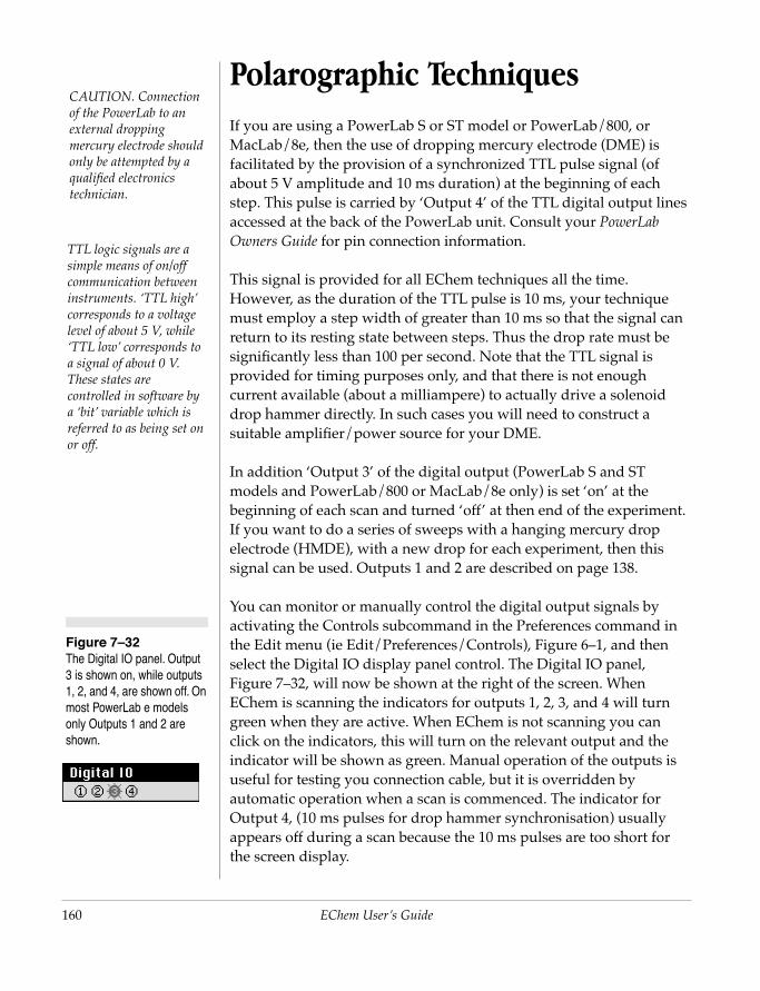
160
CAUTION. Connection of the PowerLab to an external dropping mercury electrode should only be attempted by a qualified electronics technician.
TTL logic signals are a simple means of on/off communication between instruments. ‘TTL high’ corresponds to a voltage level of about 5 V, while
Figure 7–32 The Digital IO panel. Output 3 is shown on, while outputs 1, 2, and 4, are shown off. On most PowerLab e models only Outputs 1 and 2 are shown.
Polarographic TechniquesIf you are using a PowerLab S or ST model or PowerLab/800, or MacLab/8e, then the use of dropping mercury electrode (DME) is facilitated by the provision of a synchronized TTL pulse signal (of about 5 V amplitude and 10 ms duration) at the beginning of each step. This pulse is carried by ‘Output 4’ of the TTL digital output lines accessed at the back of the PowerLab unit. Consult your PowerLab Owners Guide for pin connection information.
This signal is provided for all EChem techniques all the time. However, as the duration of the TTL pulse is 10 ms, your technique must employ a step width of greater than 10 ms so that the signal can return to its resting state between steps. Thus the drop rate must be significantly less than 100 per second. Note that the TTL signal is provided for timing purposes only, and that there is not enough current available (about a milliampere) to actually drive a solenoid drop hammer directly. In such cases you will need to construct a suitable amplifier/power source for your DME.
In addition ‘Output 3’ of the digital output (PowerLab S and ST models and PowerLab/800 or MacLab/8e only) is set ‘on’ at the beginning of each scan and turned ‘off’ at then end of the experiment. If you want to do a series of sweeps with a hanging mercury drop electrode (HMDE), with a new drop for each experiment, then this signal can be used. Outputs 1 and 2 are described on page 138.
You can monitor or manually control the digital output signals by activating the Controls subcommand in the Preferences command in
‘TTL low’ corresponds to a signal of about 0 V. These states are controlled in software by a ‘bit’ variable which is referred to as being set on or off.
EChem User’s Guide
the Edit menu (ie Edit/Preferences/Controls), Figure 6–1, and then select the Digital IO display panel control. The Digital IO panel, Figure 7–32, will now be shown at the right of the screen. When EChem is scanning the indicators for outputs 1, 2, 3, and 4 will turn green when they are active. When EChem is not scanning you can click on the indicators, this will turn on the relevant output and the indicator will be shown as green. Manual operation of the outputs is useful for testing you connection cable, but it is overridden by automatic operation when a scan is commenced. The indicator for Output 4, (10 ms pulses for drop hammer synchronisation) usually appears off during a scan because the 10 ms pulses are too short for the screen display.

EChem
User’s Guide8
C H A P T E R E I G H TAdditional Techniques
Apart from the EChem software, additional electrochemical
techniques can be performed with PowerLab using the Chart and
Scope software.
Also discussed is the use of the ADInstruments Potentiostat when
configured as a Galvanostat with Chart and Scope software.
161
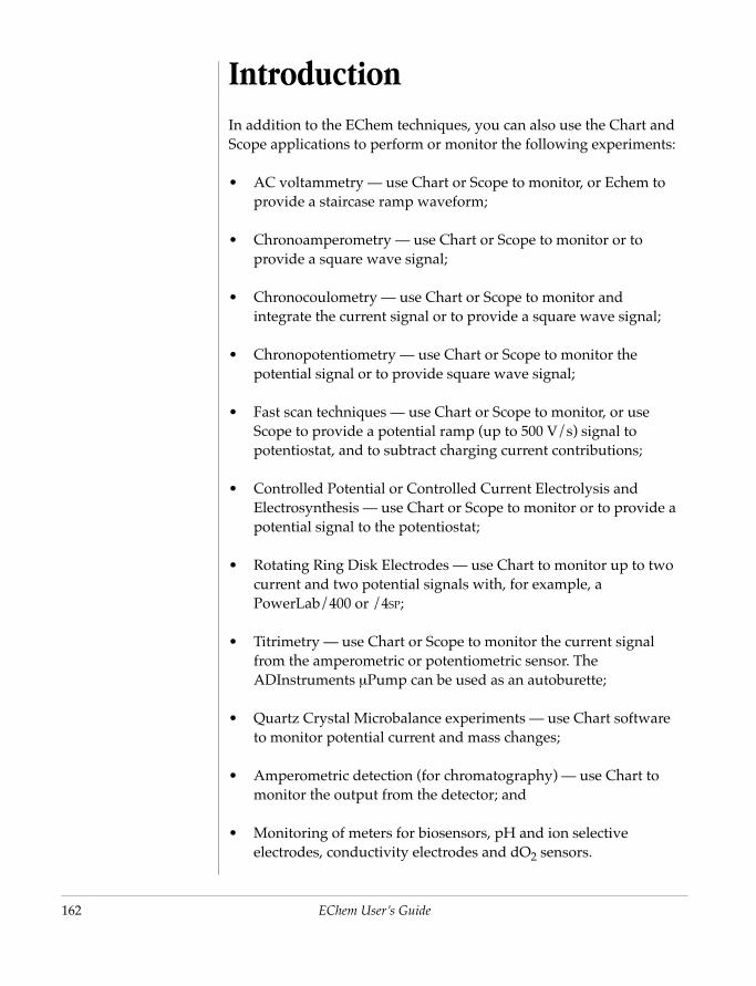
162
IntroductionIn addition to the EChem techniques, you can also use the Chart and Scope applications to perform or monitor the following experiments:
• AC voltammetry — use Chart or Scope to monitor, or Echem to provide a staircase ramp waveform;
• Chronoamperometry — use Chart or Scope to monitor or to provide a square wave signal;
• Chronocoulometry — use Chart or Scope to monitor and integrate the current signal or to provide a square wave signal;
• Chronopotentiometry — use Chart or Scope to monitor the potential signal or to provide square wave signal;
• Fast scan techniques — use Chart or Scope to monitor, or use Scope to provide a potential ramp (up to 500 V/s) signal to potentiostat, and to subtract charging current contributions;
• Controlled Potential or Controlled Current Electrolysis and Electrosynthesis — use Chart or Scope to monitor or to provide a potential signal to the potentiostat;
• Rotating Ring Disk Electrodes — use Chart to monitor up to two current and two potential signals with, for example, a PowerLab/400 or /4SP;
EChem User’s Guide
• Titrimetry — use Chart or Scope to monitor the current signal from the amperometric or potentiometric sensor. The ADInstruments µPump can be used as an autoburette;
• Quartz Crystal Microbalance experiments — use Chart software to monitor potential current and mass changes;
• Amperometric detection (for chromatography) — use Chart to monitor the output from the detector; and
• Monitoring of meters for biosensors, pH and ion selective electrodes, conductivity electrodes and dO2 sensors.

Chapter 8 — Additional Te
AC VoltammetryEChem is not specifically designed for AC voltammetric studies but there are several ways to use your PowerLab with this technique. If your existing potentiostat or waveform generator system can perform AC voltammetry then you can use your PowerLab with Chart or Scope to record the results. Your PowerLab now replaces a conventional chart recorder.
Alternatively EChem can drive such a potentiostat using the Linear Sweep or Cyclic Voltammetry modes. The potentiostat can be used to provide an AC waveform. Provided the step width of the staircase ramp generated by EChem is very much longer than the period of the AC waveform then you will get good results. For example if your AC excitation is 20 Hz, with a period of 50 ms, then you should ensure that the step width is at least 200 ms.
You can also use EChem and a PowerLab connected to a potentiostat, AC waveform generator and AC lock in amplifier. Both the EChem and the AC waveform can be summed into the potentiostat. Again make sure that the step width of the staircase ramp is much longer than the period of the AC waveform.
Fast Scan TechniquesSome techniques using microelectrodes require very fast scan rates. EChem is designed for electrochemical techniques where very high speeds are not required. The minimum step width allowed in EChem
chniques 163
is 0.1 ms, Table 7–1. You will find that this will allow scan rates of up to about 80 V/s (with PowerLab ‘s’ models) or about 30 V/s (with other PowerLab models) and still maintain adequately small step heights in the applied potential ramp. If you require faster scan rates for linear sweep or cyclic voltammetry, then you should use Scope or Chart. Both Chart and Scope incorporate Stimulator and Output Voltage commands which can be used to control the analog output of the PowerLab and to create a waveform suitable for driving a potentiostat.

164
Chart and Scope can sample up to 40,000 points per second on two channels or up to 105 points per second on one channel. You can make use of these features in a number of ways:
• if you are using a third party potentiostat capable of fast scan rates then you can use Scope as a storage oscilloscope for recording data. Up to 2560 points can be collected on one channel at a rate of up to 100 kHz, or up to 40 kHz on two channels.
• with Chart software you can monitor one channel continuously up to 200 kHz (PowerLab/4SP, /8SP, or /16SP) or 1 kHz (PowerLab/200, /400, /800). On the slower models you can also record in snapshot mode up to 16000 points at up to 100 kHz on a single channel.
Remember that Chart or Scope data is not averaged from a series of readings over a finite ‘sampling period’, as it is in EChem. Each data point corresponds to only one sampling of the signal, thus you may find that noise is more troublesome when recording at high speeds.
Read the Chart and Scope User Guides for further information on how to set up your experiment.
The PowerLab/4SP, /8SP, and /16SP models have extended high speed sampling:
• using Chart a single channel can be recorded at 200 kHz indefinitely to hard disk (or 100 kHz if using USB interface). Similarly 2 channels can be recorded at 100 kHz, 3 or 4 channels at 40 kHz, and 5–8 channels at 20 kHz, and 8–16 channels at 10
EChem User’s Guide
kHz, all continuously to hard disk.
• in both Chart and Scope the PowerLab stimulator (waveform generator) can be used at even the fastest sampling rates.
Fast Cyclic Voltammetry
Scope software has a number of features that facilitate Fast Cyclic Voltammetry (FCV). The base potential is set by using the Constant Output dialog box while the waveform is generated using the Stimulators Up & Down or Triangle waveforms (Figure 8–1). See the Scope User Guide for further details.
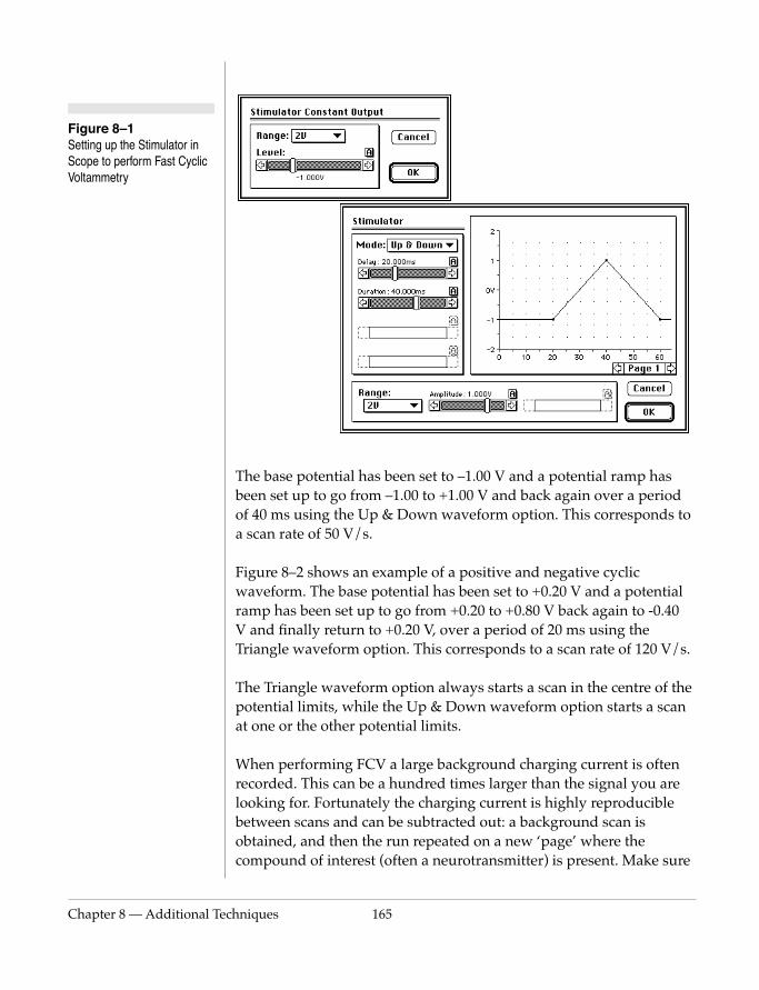
Chapter 8 — Additional Te
Figure 8–1 Setting up the Stimulator in Scope to perform Fast Cyclic Voltammetry
The base potential has been set to –1.00 V and a potential ramp has been set up to go from –1.00 to +1.00 V and back again over a period of 40 ms using the Up & Down waveform option. This corresponds to a scan rate of 50 V/s.
Figure 8–2 shows an example of a positive and negative cyclic waveform. The base potential has been set to +0.20 V and a potential ramp has been set up to go from +0.20 to +0.80 V back again to -0.40 V and finally return to +0.20 V, over a period of 20 ms using the
chniques 165
Triangle waveform option. This corresponds to a scan rate of 120 V/s.
The Triangle waveform option always starts a scan in the centre of the potential limits, while the Up & Down waveform option starts a scan at one or the other potential limits.
When performing FCV a large background charging current is often recorded. This can be a hundred times larger than the signal you are looking for. Fortunately the charging current is highly reproducible between scans and can be subtracted out: a background scan is obtained, and then the run repeated on a new ‘page’ where the compound of interest (often a neurotransmitter) is present. Make sure

166
Figure 8–2 Cyclic voltammetry using Scope and the Stimulators Triangle waveform option
that the two scans are run at the same gain setting. Select the Scope page that contains the background scan then use the Set Background command — this will subtract this scan from all other pages in the file. Use the Don't Subtract Background command to cancel subtraction, and the Clear Background de-identifies the background page. See the Scope User’s Guide for more information.
Low Current ExperimentsSome experiments using microelectrodes (especially when used in
EChem User’s Guide
organic solvents, or for in vivo studies) require the measurement of extremely small currents. You can use the PowerLab system to perform electrochemistry on such systems provided that you have a suitable potentiostat available.
If you are using microelectrodes the you may need the ADInstruments Picostat™ (under development at the time of writing) This has a thousand times the sensitivity of the ADInstruments Potentiostat. To minimize interference from noise, try to position the Picostat as close to the electrodes as possible, and shield the experiment well (usually by enclosure in a Faraday cage).

Chapter 8 — Additional Te
Another suitable instrument for microelectrode work is the BAS Low Current Module (available from Bioanalytical Systems Inc.). This system can be supplied with its own Faraday cage (the BAS C–2 Cell Stand) and has current ranges from 10 pA/V to 1 µA/V, with a maximum current of 12 µA. The current signal is amplified near the electrodes inside the Faraday cage. Your ADInstruments dealer can supply the necessary cables to connect your PowerLab unit to this system (see Chapter 9). Please note that the Low Current Module is directly connected to the PowerLab unit — no other potentiostat is required.
Chronoamperometry These techniques require that a constant potential is maintained for a defined period while the current is monitored (chronoampero-metry). If the current signal is integrated with respect to time then the total charge transferred at the electrode can be calculated (chrono-coulometry).
For these techniques Chart and Scope (supplied with the PowerLab unit) can be used. PowerLab with Chart or Scope will allow you to perform Single, Double and even Multi-Step Chronoamperometry, with data collection taking place in milliseconds or over hours or even days if need be.
Chronoamperometry and Chart
Chart software can be used to output a constant potential (up to
chniques 167
±10 V) with a suitable potentiostat equipped with an external input (or the ADinstruments Potentiostat). The Timed Events (Setup menu) feature can be used to keep the potential constant for a fixed period of time, or even to drive the reaction backwards after the initial oxidation/reduction.
To adjust the potential you will first need to select the range by choosing the Constant Voltage command in the Setup menu to activate the Constant Output dialog, Figure 8–3. You can set the control voltage sent to the potentiostat by setting the slider bar or entering a value after clicking the A-button. The slider control, and the direct text entry available with A-button, both offer 12 bit resolution (0.024%) within each range (selected by the pull down).

168
Figure 8–3 The Constant Output Dialog box.
At the time of writing the Timed Events feature was only available for Macintosh systems.
At the time of writing the control of the Stimulator with Chart software on Windows computers was still under development. There may be significant differences in its use.
This equates to 1 mV resolution if you use the ±2 V range, which is suitable for most experiments employing aqueous solutions.
If you are using a bipotentiostat with a PowerLab S series model then clicking the Independent radio button, Figure 8–3, allows you to set two output voltages which can be sent to the two external inputs of the bipotentiostat.
The Chart software Stimulator command (in the Setup menu) can also be used to set up pulses, stepped pulses, and staircase ramp waveforms which the potentiostat will follow. PowerLab S series models can also be configured in Chart software to provide sinusoidal and triangular wavefunctions).
Output Voltage control for PowerLab S series models)
Output Voltage control for PowerLab e series models
EChem User’s Guide
You can also use the Timed Events feature (Setup menu) to adjust the current at predetermined time intervals after the start of recording. For example the settings shown in Figure 8–4 will maintain a potential of 1.25 V for 30 minutes after which the potential will be decreased to 0.50 V in order to reverse the reaction, resulting in a Double Step Chronoamperometric experiment. Any number of steps at any potential could be set up with this feature.
Timed Events can be slightly delayed by up to (0.1 s) depending on the model of computer and what else is happening. For fast charging and discharging systems it is better to use the Chart Stimulator.
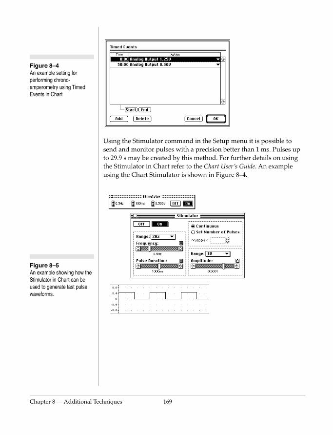
Chapter 8 — Additional Te
Figure 8–5 An example showing how the Stimulator in Chart can be used to generate fast pulse waveforms.
Figure 8–4 An example setting for performing chrono-amperometry using Timed Events in Chart
Using the Stimulator command in the Setup menu it is possible to send and monitor pulses with a precision better than 1 ms. Pulses up to 29.9 s may be created by this method. For further details on using the Stimulator in Chart refer to the Chart User’s Guide. An example using the Chart Stimulator is shown in Figure 8–4.
chniques 169
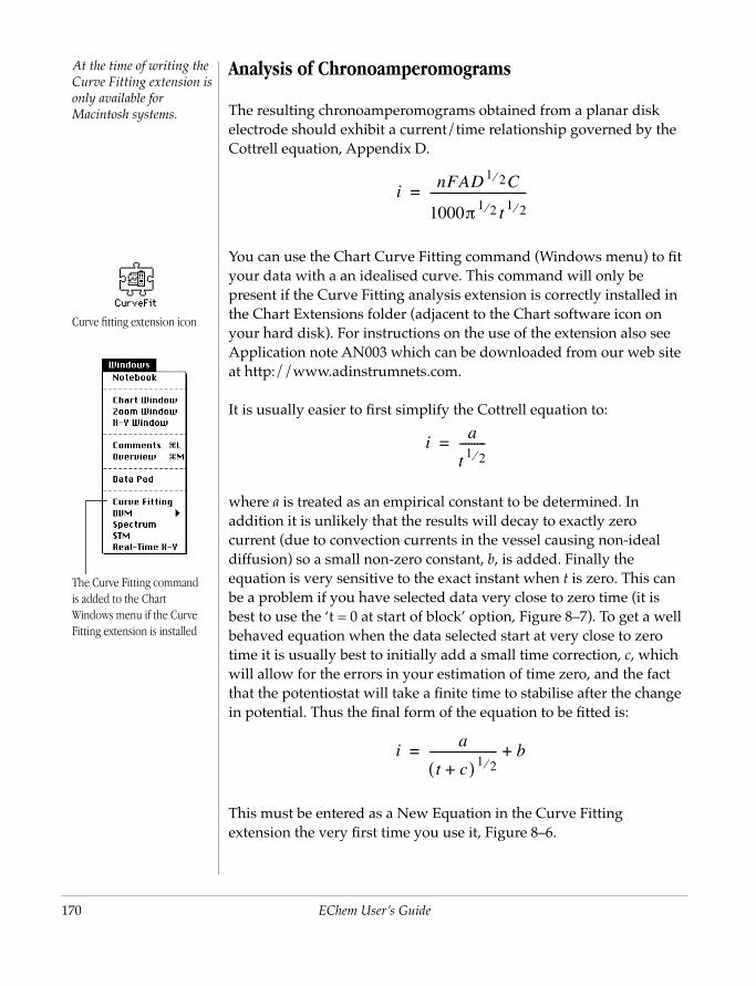
170
Curve fitting extension icon
The Curve Fitting command is added to the Chart Windows menu if the Curve Fitting extension is installed
At the time of writing the Curve Fitting extension is only available for Macintosh systems.
Analysis of Chronoamperomograms
The resulting chronoamperomograms obtained from a planar disk electrode should exhibit a current/time relationship governed by the Cottrell equation, Appendix D.
You can use the Chart Curve Fitting command (Windows menu) to fit your data with a an idealised curve. This command will only be present if the Curve Fitting analysis extension is correctly installed in the Chart Extensions folder (adjacent to the Chart software icon on your hard disk). For instructions on the use of the extension also see Application note AN003 which can be downloaded from our web site at http://www.adinstrumnets.com.
It is usually easier to first simplify the Cottrell equation to:
where a is treated as an empirical constant to be determined. In addition it is unlikely that the results will decay to exactly zero current (due to convection currents in the vessel causing non-ideal diffusion) so a small non-zero constant, b, is added. Finally the equation is very sensitive to the exact instant when t is zero. This can be a problem if you have selected data very close to zero time (it is best to use the ‘t = 0 at start of block’ option, Figure 8–7). To get a well
inFAD 1 2⁄ C
1000π 1 2⁄ t 1 2⁄---------------------------------=
ia
t 1 2⁄---------=
EChem User’s Guide
behaved equation when the data selected start at very close to zero time it is usually best to initially add a small time correction, c, which will allow for the errors in your estimation of time zero, and the fact that the potentiostat will take a finite time to stabilise after the change in potential. Thus the final form of the equation to be fitted is:
This must be entered as a New Equation in the Curve Fitting extension the very first time you use it, Figure 8–6.
ia
t c+( ) 1 2⁄----------------------- b+=
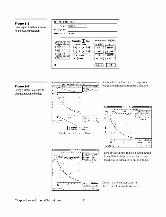
Chapter 8 — Additional Te
Figure 8–7 Fitting a Cottrell equation to chronoamperometric data
First lock the value for c, then type in guesses for a and b until an approximate fit is obtained
Usually use ‘t=0 at start of block’
Figure 8–6 Entering an equation suitable for the Cottrell equation
chniques 171
Iterate by clicking the Fit button, refining a and b only. If the initial guesses are close enough then better vales for a and b will be obtained.
Unlock c, and iterate again. A curve of even better fit should be obtained.
172
CAUTION If you are using a high compliance potentiostat or galvanostat remember that dangerous or even lethal potentials may be generated across the electrodes. Read your potentiostat/ galvanostat manual carefully to establish safe working procedures, and always isolate the cell before disconnecting the electrodes. The potential at which the potentiostat is set refers to the potential between the working and reference electrodes, the potential between the auxiliary and working electrodes may be many times greater!
After the file is saved the equation will be available whenever you open Chart data file on the computer or even when you transfer the data file to another computer. Some trial and error will be involved while you make guesses that are suitable for the initial values to commence iteration.
Because of the discontinuity that occurs when the denominator is zero problems can occur if the selected data starts at zero time (or close to zero time). In this case first try fixing c to a small positive value, and iterating for better values of a and b. Usually your data selection should not include data points very close to zero time (the potentiostat will require some time to settle — remember to have the potentiostat low pass filters turned off otherwise you may only be measuring the filter response time!), nor points taken at very long times when convection aided diffusion will produce non-ideal behaviour. The exact time period that is suitable will depend on the size of the electrode and the quality of the potentiostat and some trial and error to determine the best time interval will be required. After the better estimates for a and b have been determined c can be set free to refine during the next iteration cycle, Figure 8–7
Chronoamperometry and Scope
For chronoamperometric measurements, where you need to overlay the results of successive experiments, Scope will generally be the program of choice.
The total length of the experiment is chosen in the Time Base panel (128 s is usually sufficient, this is given by the 100 s setting). Up to
EChem User’s Guide
2560 data points can be collected in this period. The base potential is adjusted with the Output Voltage command (Setup menu) and is similar in function to the corresponding Chart software control shown in Figure 8–3.
The potential that will cause the reaction to proceed (and the time that it will be applied) is set using the Stimulator command in the Setup menu. In the example shown in Figure 8–9, after a period of 10 s at the base potential, two 30 s pulses of –0.70 V are to be applied each followed by a 30 s return to the base potential.
The experiment is usually first done on a blank solution containing only electrolyte, followed by a sample solution containing the
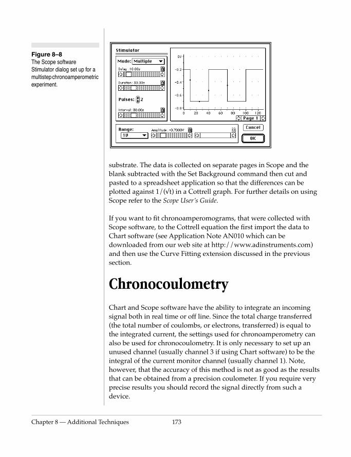
Chapter 8 — Additional Te
Figure 8–8 The Scope software Stimulator dialog set up for a multistep chronoamperometric experiment.
substrate. The data is collected on separate pages in Scope and the blank subtracted with the Set Background command then cut and pasted to a spreadsheet application so that the differences can be plotted against 1/(√t) in a Cottrell graph. For further details on using Scope refer to the Scope User’s Guide.
If you want to fit chronoamperomograms, that were collected with Scope software, to the Cottrell equation the first import the data to Chart software (see Application Note AN010 which can be downloaded from our web site at http://www.adinstruments.com) and then use the Curve Fitting extension discussed in the previous section.
Chronocoulometry
chniques 173
Chart and Scope software have the ability to integrate an incoming signal both in real time or off line. Since the total charge transferred (the total number of coulombs, or electrons, transferred) is equal to the integrated current, the settings used for chronoamperometry can also be used for chronocoulometry. It is only necessary to set up an unused channel (usually channel 3 if using Chart software) to be the integral of the current monitor channel (usually channel 1). Note, however, that the accuracy of this method is not as good as the results that can be obtained from a precision coulometer. If you require very precise results you should record the signal directly from such a device.
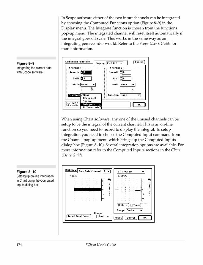
174
Figure 8–9 Integrating the current data with Scope software.
Figure 8–10 Setting up on-line integration in Chart using the Computed Inputs dialog box
In Scope software either of the two input channels can be integrated by choosing the Computed Functions option (Figure 8–9) in the Display menu. The Integrate function is chosen from the functions pop-up menu. The integrated channel will reset itself automatically if the integral goes off scale. This works in the same way as an integrating pen recorder would. Refer to the Scope User’s Guide for more information.
When using Chart software, any one of the unused channels can be setup to be the integral of the current channel. This is an on-line function so you need to record to display the integral. To setup integration you need to choose the Computed Input command from the Channel pop-up menu which brings up the Computed Inputs dialog box (Figure 8–10). Several integration options are available. For more information refer to the Computed Inputs sections in the Chart User’s Guide.
EChem User’s Guide
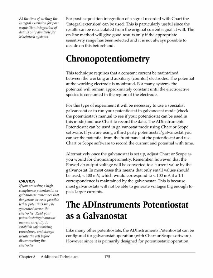
Chapter 8 — Additional Te
CAUTION If you are using a high compliance potentiostat or galvanostat remember that dangerous or even possible lethal potentials may be generated across the electrodes. Read your potentiostat/galvanostat manual carefully to establish safe working procedures, and always isolate the cell before disconnecting the electrodes.
At the time of writing the Integral extension for post acquisition integration of data is only available for Macintosh systems.
For post-acquisition integration of a signal recorded with Chart the ‘Integral extension’ can be used. This is particularly useful since the results can be recalculated from the original current signal at will. The on-line method will give good results only if the appropriate sensitivity range has been selected and it is not always possible to decide on this beforehand.
Chronopotentiometry This technique requires that a constant current be maintained between the working and auxiliary (counter) electrodes. The potential at the working electrode is monitored. For many systems the potential will remain approximately constant until the electroactive species is consumed in the region of the electrode.
For this type of experiment it will be necessary to use a specialist galvanostat or to run your potentiostat in galvanostat mode (check the potentiostat's manual to see if your potentiostat can be used in this mode) and use Chart to record the data. The ADinstruments Potentiostat can be used in galvanostat mode using Chart or Scope software. If you are using a third party potentiostat/galvanostat you can set the potential from the front panel of the potentiostat and use Chart or Scope software to record the current and potential with time.
Alternatively once the galvanostat is set up, adjust Chart or Scope as you would for chronoamperometry. Remember, however, that the PowerLab output voltage will be converted to a current value by the galvanostat. In most cases this means that only small values should be used, < 100 mV, which would correspond to < 100 mA if a 1:1
chniques 175
correspondence is maintained by the galvanostat. This is because most galvanostats will not be able to generate voltages big enough to pass larger currents.
The ADInstruments Potentiostat as a GalvanostatLike many other potentiostats, the ADInstruments Potentiostat can be configured for galvanostat operation (with Chart or Scope software). However since it is primarily designed for potentiostatic operation

176
Figure 8–11 Setting up the ADinstruments Potentiostat in galvanostat mode.
At the time of writing the control of the Potentiostat with Chart software on Windows computers was still under development.
you will need to take some extra care when setting it up as a galvanostat.
First switch to the galvanostat mode of operation. Choose the Potentiostat item in the Channel menu to open the control window and turn on the Galvanostat and Dummy radio buttons, Figure 8–11.
The default setting is for zero current on the 100 mA range. It is likely that there will be a small residual offset at this setting which will cause the Potentiostat/Galvanostat to go off scale (over 10 V) in standby mode (as it is connected to the internal 100 kΩ dummy cell).
First find the Potentiostat menu item in the Chart software Channel menu
At each PowerLab control Output Voltage setting there are four current range settings available
Display area showing potential signal
EChem User’s Guide
Try selecting the 1 µA or 10 µA range, where the offset will be correspondingly smaller, and the signal should come on screen and be close to zero volts.
The PowerLab control voltage can be set using the Chart software Output Voltage command in the Setup menu. You can select a range of 100 mV to 10 V in 1:2:5 increments on most models, or 200 mV to 10 V on PowerLab /200 and /400 models, Figure 8–3.
At each of the Output Voltage range settings the ADInstruments Potentiostat/ Galvanostat offers four current range settings when in Galvanostat mode, Table 8–1. The most accurate control is achieved by using the largest possible Output Voltage range with the smallest
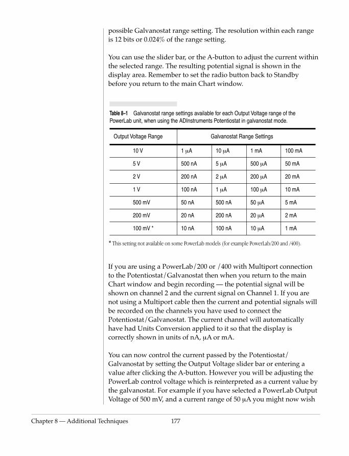
Chapter 8 — Additional Te
possible Galvanostat range setting. The resolution within each range is 12 bits or 0.024% of the range setting.
You can use the slider bar, or the A-button to adjust the current within the selected range. The resulting potential signal is shown in the display area. Remember to set the radio button back to Standby before you return to the main Chart window.
If you are using a PowerLab/200 or /400 with Multiport connection to the Potentiostat/Galvanostat then when you return to the main Chart window and begin recording — the potential signal will be
Table 8–1 Galvanostat range settings available for each Output Voltage range of the PowerLab unit, when using the ADInstruments Potentiostat in galvanostat mode.
Output Voltage Range Galvanostat Range Settings
10 V 1 µA 10 µA 1 mA 100 mA
5 V 500 nA 5 µA 500 µA 50 mA
2 V 200 nA 2 µA 200 µA 20 mA
1 V 100 nA 1 µA 100 µA 10 mA
500 mV 50 nA 500 nA 50 µA 5 mA
200 mV 20 nA 200 nA 20 µA 2 mA
100 mV * 10 nA 100 nA 10 µA 1 mA
* This setting not available on some PowerLab models (for example PowerLab/200 and /400).
chniques 177
shown on channel 2 and the current signal on Channel 1. If you are not using a Multiport cable then the current and potential signals will be recorded on the channels you have used to connect the Potentiostat/Galvanostat. The current channel will automatically have had Units Conversion applied to it so that the display is correctly shown in units of nA, µA or mA.
You can now control the current passed by the Potentiostat/ Galvanostat by setting the Output Voltage slider bar or entering a value after clicking the A-button. However you will be adjusting the PowerLab control voltage which is reinterpreted as a current value by the galvanostat. For example if you have selected a PowerLab Output Voltage of 500 mV, and a current range of 50 µA you might now wish
178
to do an experiment where the current is held at a constant 35 µA (or 35/50 × 100 = 70% of the range setting). You should now set the slider control of the Output Voltage control to a value of 70% of 500 mV, that is to 350 mV. Remember that the use of + and – voltages determine the direction of current flow (into or out of the working electrode).
The Chart software Stimulator command (Setup menu) can also be used to set up pulses, stepped pulses, and staircase ramp waveforms which the galvanostat will follow (PowerLab/4SP, /8SP, or /16SP models can also be configured in Chart software to provide sinusoidal and triangular wavefunctions). You can also use the Timed Events feature (Setup menu) to adjust the current at predetermined time intervals after the start of recording.
Operation of the Potentiostat/Galvanostat with Scope software is similar but a wider variety of waveforms can be used.
Consult the Chart and Scope User’s Guides for more details of the Output Voltage, Stimulator, and Timed Events features.
Controlled Potential Electrolysis and ElectrosynthesisThese techniques are essentially the same as chronoamperometry. A constant potential is applied at the working electrode which is sufficient to oxidize or reduce the substrate. As the electrolysis continues the substrate is eventually completely consumed and the current will decrease to a residual value. Both the potential and the
EChem User’s Guide
current flow can be monitored with Chart in the same way as for chronoamperometry. The integrated current (i.e. the total charge transferred) can also be determined which can be used to determine the extent of reaction.
A potential should be chosen which is at least 50 – 200 mV more oxidizing (or reducing) than the half potential in order to ensure complete reaction of the substrate. It is important to separate the auxiliary (counter) electrode from the electrochemical cell by means of a salt bridge. This is due to the build up of reduction products in the region of the auxiliary electrode which could react with the products of oxidation at the working electrode (or conversely
Chapter 8 — Additional Te
products of oxidation will build up around the auxiliary electrode if reduction is taking place at the working electrode). The working electrode is constructed to have a large surface area so that a greater amount of material can be electrolyzed in a small time, thus a plate or gauze electrode is usually chosen.
It is usual to stir the solution during electrolysis in order to bring a fresh supply of substrate into contact with the working electrode.
For the conversion of large amounts of substrate (> 100 mg) in reasonable times relatively high currents must be passed through the cell. A potentiostat capable of a maximum current of at least 100 mA, or even 1 A is required. For the electrosynthesis of organic compounds in highly resistive non-aqueous solvents the addition of a large amount of electrolyte is necessary to sustain the current flow (which can sometimes lead to difficulties in later separation of the product), as is the use of a high compliance potentiostat. For studies using water as the solvent the addition of a small quantity of acid (or base) can increase the conductivity of the cell greatly, without having to add large amounts of electrolyte.
Controlled Current Electrolysis and ElectrosynthesisThese techniques are essentially the same as chronopotentiometry and require the use of a galvanostat (or constant current source and voltmeter). A constant current is applied between the working and auxiliary electrodes and the potential at the working electrode is
chniques 179
monitored as the substrate is oxidized or reduced. As the electrolysis continues the substrate is eventually completely consumed and the potential will alter as the galvanostat tries to maintain a constant current. Both the potential and the current flow can be monitored with Chart software. The integrated current (i.e. the total charge transferred) can also be determined which can be used to determine the extent of reaction.
Electrosynthesis reactions are often more quickly carried out under constant current conditions (especially if there are no competing redox reactions at nearby potentials) than under constant potential conditions.

180
It is important to limit the current so that the potential stays within the compliance voltage of the galvanostat, at least until the reaction of interest is complete.
Many potentiostats can be used in galvanostat mode — consult the instrument manual to see if this is possible. The use of the ADInstruments Potentiostat in galvanostat mode is discussed above: See “The ADInstruments Potentiostat as a Galvanostat” on page 175.
Rotating Ring Disk ElectrodesA rotating ring disk electrode (RRDE) consists of two electrodes: an inner circular cross section electrode; and an outer, concentric, annular electrode. Both the disk and the ring can be controlled independently by two separate potentiostats or with a bipotentiostat. Rotation of the electrode causes hydrodynamic flow such that the solution is moved onto the disk from the bulk solvent then pushed outwards towards the ring. Thus the RRDE can be used to measure rates of various redox reactions, using the ring as a detector and the disk as a generator of various electroactive substances.
Much RRDE work will require at least a four channel PowerLab unit (for example a PowerLab/400) as the potential and current flows of both (or either) the ring or disk will need to be monitored.
A typical experiment would use a PowerLab/400 with Chart to record the results. The current at the ring is held at a constant oxidizing potential to detect any reduced species formed at the disk. The disk potential is swept over a range of potentials in order to
EChem User’s Guide
generate various reduced species in solution. Because the ring potential is held constant it does not need to be monitored. But we will need to plot both the disk and ring currents against the disk potential so each of these must be recorded. The Chart X-Y Window command (Windows menu) can be used to plot the results on one channel versus another.
Amperometric TitrimetryTitrations can be performed in an electrochemical cell where the working electrode is held at a constant potential while the current is
Chapter 8 — Additional Te
monitored. As the electroactive species is consumed during the titration the current decreases.
The ADInstruments µPump, can be used to deliver 50 µL aliquots of titrant to a vessel with a coefficient of variability of 0.3%. It is suitable (after calibration) for performing titrations on a scale similar to that used with a conventional 25 or 50 mL burette. Monitoring such a titration is best achieved with Chart software, plotting volume and current flow on separate channels. Chart also has the ability to perform XY plots so that current can be plotted against volume of titrant added.
Liquid Chromatography DetectorsElectrochemical detection can be an extremely sensitive technique for liquid and high–pressure liquid chromatography (LC and HPLC). The method is essentially chronoamperometry on a flowing sample. A flow–through cell must be purchased or constructed.
Chart can be set up to drive the potentiostat at a constant potential for an indefinite period. Alternatively the potentiostat can be set to provide a fixed potential. The potential is chosen such that the substrate will be oxidised or reduced as it passes through the electrochemical cell. The current is monitored continuously. As the substrate passes through the cell an increase in the current occurs, the current then peaks and subsides as the substrate is pushed out of the cell by new carrier solution.
chniques 181
Chart can also be used to monitor the outputs of other detectors connected to other channels of the PowerLab. Thus using a PowerLab/400 you could monitor output from an electrochemical, uv-visible, refractive index, and fluorescence detector, simultaneously. In addition four virtual channels of data can be constructed using the computed functions dialog to monitor the integrated signals (or their differentials) from each of the detectors. Refer to the Chart User's Guide for further details.
For more extensive chromatographic use, PowerChrom software is also available for use with PowerLab units. It can acquire and analyze
182
data, and supports autosamplers and fraction collectors. The ADinstruments Potentiostat can be used as a low cost electrochemical detector for chromatography systems when used in conjunction with Chart or PowerChrom software. Ask your ADInstruments dealer for more information.
BiosensorsBiosensors are usually of the potentiometric, amperometric or conductiometric varieties (see the following sections). Usually ordinary pH meters or high impedance voltmeters can be used for the potentiometric type. The amperometric variety usually require a special meter that has an adjustable polarizing potential and a variable gain ranges suitable for the currents being measured (see Appendix F). The conductiometric types may work with an ordinary conductivity meter but may have special requirements in terms of the frequency of AC excitation or the range of conductances to be measured. Any ‘biosensor’ meter with an analog recorder output can be connected to a PowerLab unit.
Potentiometric sensorsAs their name suggests these sensors measure potential, and there output can always be monitored in units of millivolts or volts. In some cases it is more convenient to convert this signal to alternative units such a pH or log[Na] to give a more direct indication of the type of measurement being carried out. Virtually all these sensors can be monitored by connection to a pH meter or other high impedance
EChem User’s Guide
voltmeter.
pH Electrodes
The impedance of the PowerLab inputs is 106 Ω which is unsuitable for direct connection to the very high impedance signals produced by glass pH electrodes. For these electrodes a high impedance preamplifier (a pH or ISE meter with an impedance of >1012 Ω) must be used between the electrodes and the PowerLab. The ADinstruments pH Amp is also suitable for most pH and
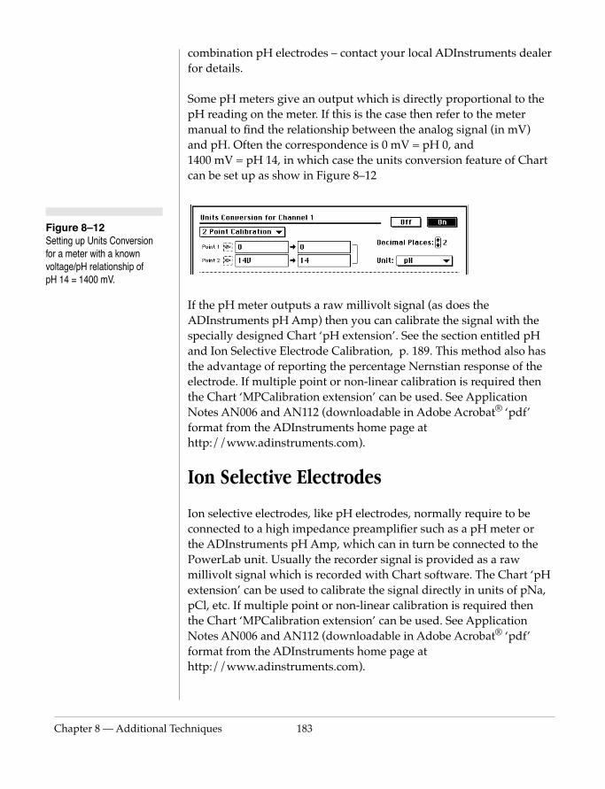
Chapter 8 — Additional Te
Figure 8–12 Setting up Units Conversion for a meter with a known voltage/pH relationship of pH 14 = 1400 mV.
combination pH electrodes – contact your local ADInstruments dealer for details.
Some pH meters give an output which is directly proportional to the pH reading on the meter. If this is the case then refer to the meter manual to find the relationship between the analog signal (in mV) and pH. Often the correspondence is 0 mV = pH 0, and 1400 mV = pH 14, in which case the units conversion feature of Chart can be set up as show in Figure 8–12
If the pH meter outputs a raw millivolt signal (as does the ADInstruments pH Amp) then you can calibrate the signal with the specially designed Chart ‘pH extension’. See the section entitled pH and Ion Selective Electrode Calibration, p. 189. This method also has the advantage of reporting the percentage Nernstian response of the electrode. If multiple point or non-linear calibration is required then the Chart ‘MPCalibration extension’ can be used. See Application Notes AN006 and AN112 (downloadable in Adobe Acrobat® ‘pdf’ format from the ADInstruments home page at http://www.adinstruments.com).
Ion Selective Electrodes
chniques 183
Ion selective electrodes, like pH electrodes, normally require to be connected to a high impedance preamplifier such as a pH meter or the ADInstruments pH Amp, which can in turn be connected to the PowerLab unit. Usually the recorder signal is provided as a raw millivolt signal which is recorded with Chart software. The Chart ‘pH extension’ can be used to calibrate the signal directly in units of pNa, pCl, etc. If multiple point or non-linear calibration is required then the Chart ‘MPCalibration extension’ can be used. See Application Notes AN006 and AN112 (downloadable in Adobe Acrobat® ‘pdf’ format from the ADInstruments home page at http://www.adinstruments.com).
184
Potentiometric Redox Electrodes
Depending on the design of the electrode it may be possible to connect a reference and redox electrode directly to the PowerLab inputs. However, for best quality results it is usually better to use a high impedance preamplifier such as a pH meter or the ADInstruments pH Amp, which can in turn be connected to the PowerLab unit. Chart software is usually the best choice to record the signal.
Dissolved CO2 and NH3 Electrodes
These electrodes measure the pH of an internal solution which is separated from the bulk solution by a gas permeable membrane. As CO2 (or NH3) concentration equilibrates on either side of the membrane, the pH of the internal solution will change. The resulting signal is usually measured with a conventional pH meter. The recorder signal of the pH meter can be monitored with Chart software on a PowerLab unit. The Units Conversion feature of Chart can be used to perform two point calibration of the signal which is satisfactory for most uses. If multiple point or non-linear calibration is required then the Chart ‘MPCalibration extension’ can be used. See Application Note AN112 (downloadable in Adobe Acrobat® ‘pdf’ format from http://www.adinstruments.com).
Electrode Behaviour
The behaviour of an ideal pH, or ion sensitive, electrode is
EChem User’s Guide
characterised by the Nernst equation. This describes the relationship between observed potential and ion activity.
where
E is the observed potential (in volts)E0 is the potential when pY is zeroR is the gas constant (8.314 J K-1 mol-1)T is the temperature in KelvinF is the Faraday constant (96487 C mol-1)
E E0RTnF------- pY–=
Chapter 8 — Additional Te
At the time of writing the MP Calibration extension is only available for Macintosh systems.
n is the number of electrons transferred at the electrode(usually the charge of the ion)
pY = –log10[Y] where [Y] is the activity of the ionic species, Y(for a pH electrode pY = pH)
If pY is plotted against E then a straight line should be obtained of intercept E0 and a slope of –(RT/nF). For pH measurements (n=+1) at 25°C and the expression RT/nF has a value of 59.16 mV.
If two solutions of known pY are measured then these values can be used to construct a graph of a straight line to determine E0 and the slope. The percentage Nernstian response of the electrode is given by:
where slopeobserved is the observed slope and slopecalculated = (–RT/nF)
Such a graph, with the Nernstian response is calculated by the Chart pH extension.
High quality pH electrodes will have a response in the range 95 – 102%. Cheaper, older, or poorly maintained, electrodes will most likely have a response below this range. Ion selective electrodes exhibit a wider variation which should be taken into account when characterising electrode types.
Non-Linear Multiple Point Calibration
response100 slopeobserved×
slopecalculated-----------------------------------------------=
chniques 185
Both single and two point calibration assume that the electrode has a linear response to ion activity. Experimentally there will always be some deviation from linearity in the response. This is most noticeable at very high or low concentrations. In these instances a non-linear calibration technique must be used for accurate work.
If you need to calibrate an electrode directly in terms of ionic concentration (or log of concentration) rather than activity, a non-linear calibration is also needed. The Chart Mutipoint calibration extension can perform this sort of non-linear calibration.
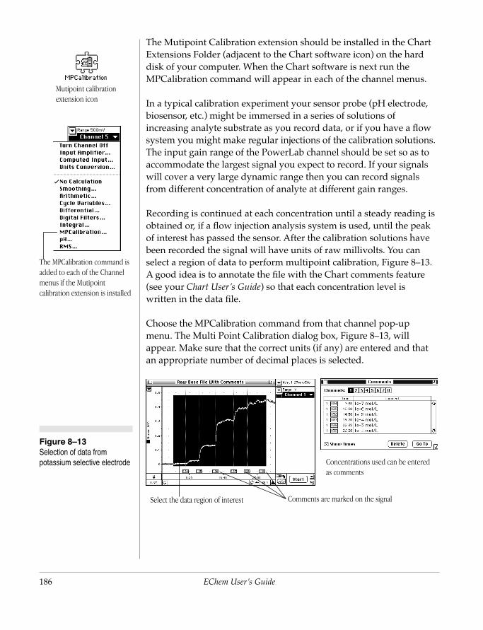
186
Mutipoint calibration extension icon
Figure 8–13 Selection of data from potassium selective electrode
The Mutipoint Calibration extension should be installed in the Chart Extensions Folder (adjacent to the Chart software icon) on the hard disk of your computer. When the Chart software is next run the MPCalibration command will appear in each of the channel menus.
In a typical calibration experiment your sensor probe (pH electrode, biosensor, etc.) might be immersed in a series of solutions of increasing analyte substrate as you record data, or if you have a flow system you might make regular injections of the calibration solutions. The input gain range of the PowerLab channel should be set so as to accommodate the largest signal you expect to record. If your signals will cover a very large dynamic range then you can record signals from different concentration of analyte at different gain ranges.
Recording is continued at each concentration until a steady reading is obtained or, if a flow injection analysis system is used, until the peak of interest has passed the sensor. After the calibration solutions have been recorded the signal will have units of raw millivolts. You can select a region of data to perform multipoint calibration, Figure 8–13. A good idea is to annotate the file with the Chart comments feature (see your Chart User’s Guide) so that each concentration level is written in the data file.
Choose the MPCalibration command from that channel pop-up menu. The Multi Point Calibration dialog box, Figure 8–13, will appear. Make sure that the correct units (if any) are entered and that an appropriate number of decimal places is selected.
The MPCalibration command is added to each of the Channel menus if the Mutipoint calibration extension is installed
EChem User’s Guide
Select the data region of interest
Concentrations used can be entered as comments
Comments are marked on the signal
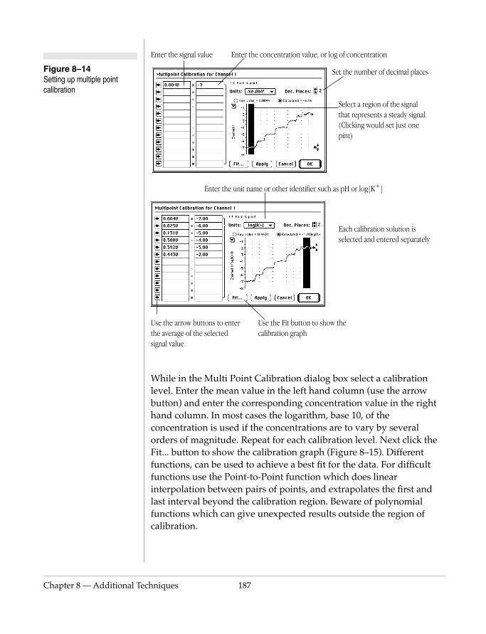
Chapter 8 — Additional Te
Figure 8–14 Setting up multiple point calibration
While in the Multi Point Calibration dialog box select a calibration level. Enter the mean value in the left hand column (use the arrow button) and enter the corresponding concentration value in the right
Select a region of the signal that represents a steady signal. (Clicking would set just one pint)
Each calibration solution is selected and entered separately
Use the arrow buttons to enter the average of the selected signal value
Enter the unit name or other identifier such as pH or log[K+]
Set the number of decimal places
Use the Fit button to show the calibration graph
Enter the signal value Enter the concentration value, or log of concentration
chniques 187
hand column. In most cases the logarithm, base 10, of the concentration is used if the concentrations are to vary by several orders of magnitude. Repeat for each calibration level. Next click the Fit... button to show the calibration graph (Figure 8–15). Different functions, can be used to achieve a best fit for the data. For difficult functions use the Point-to-Point function which does linear interpolation between pairs of points, and extrapolates the first and last interval beyond the calibration region. Beware of polynomial functions which can give unexpected results outside the region of calibration.
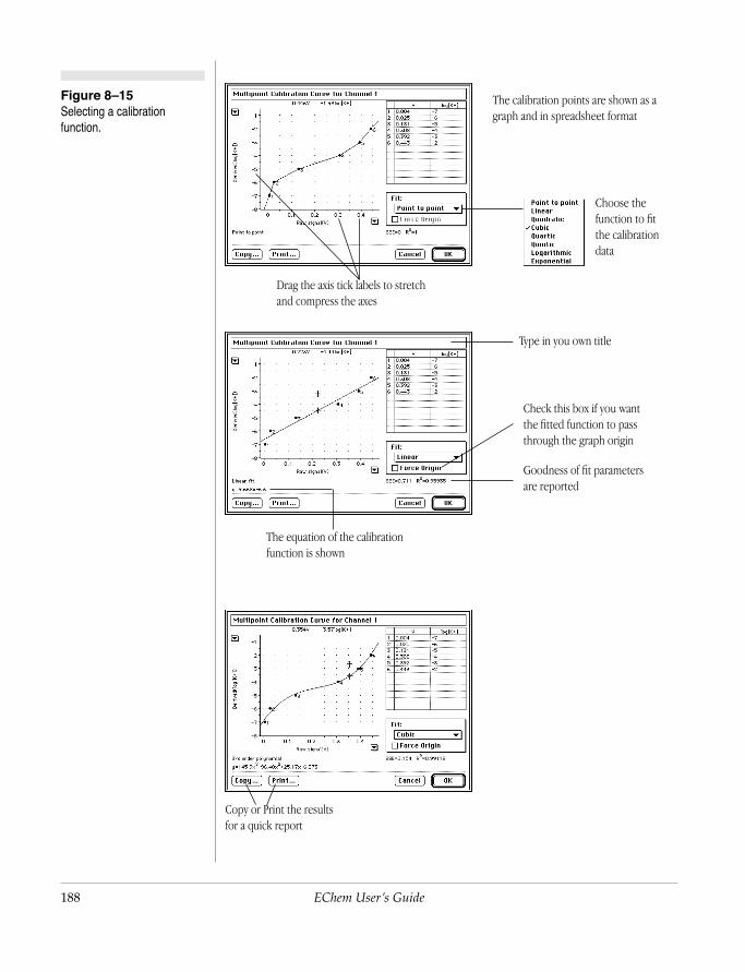
188
Figure 8–15 Selecting a calibration function.
The calibration points are shown as a graph and in spreadsheet format
Choose the function to fit the calibration data
The equation of the calibration function is shown
Goodness of fit parameters are reported
Drag the axis tick labels to stretch and compress the axes
Type in you own title
Check this box if you want the fitted function to pass through the graph origin
EChem User’s Guide
Copy or Print the results for a quick report
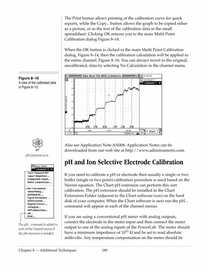
Chapter 8 — Additional Te
pH extension icon
The pH... command is added to each of the Channel menus if the pH extension is installed
Figure 8–16 A view of the calibrated data in Figure 8–13.
The Print button allows printing of the calibration curve for quick reports, while the Copy... button allows the graph to be copied either as a picture, or as the text of the calibration data in the small spreadsheet. Clicking OK returns you to the main Multi Point Calibration dialog Figure 8–14.
When the OK button is clicked in the main Multi Point Calibration dialog, Figure 8–14, then the calibration calculation will be applied to the entire channel, Figure 8–16. You can always revert to the original, uncalibrated, data by selecting No Calculation in the channel menu.
Also see Application Note AN006. Application Notes can be downloaded from our web site at http://www.adinstruments.com.
pH and Ion Selective Electrode Calibration
chniques 189
If you need to calibrate a pH or electrode then usually a single or two buffer (single or two point) calibration procedure is used based on the Nernst equation. The Chart pH extension can perform this sort calibration. The pH extension should be installed in the Chart Extensions Folder (adjacent to the Chart software icon) on the hard disk of your computer. When the Chart software is next run the pH... command will appear in each of the channel menus.
If you are using a conventional pH meter with analog outputs, connect the electrode to the meter input and then connect the meter output to one of the analog inputs of the PowerLab. The meter should have a minimum impedance of 1012 Ω and be set to read absolute millivolts. Any temperature compensation on the meter should be
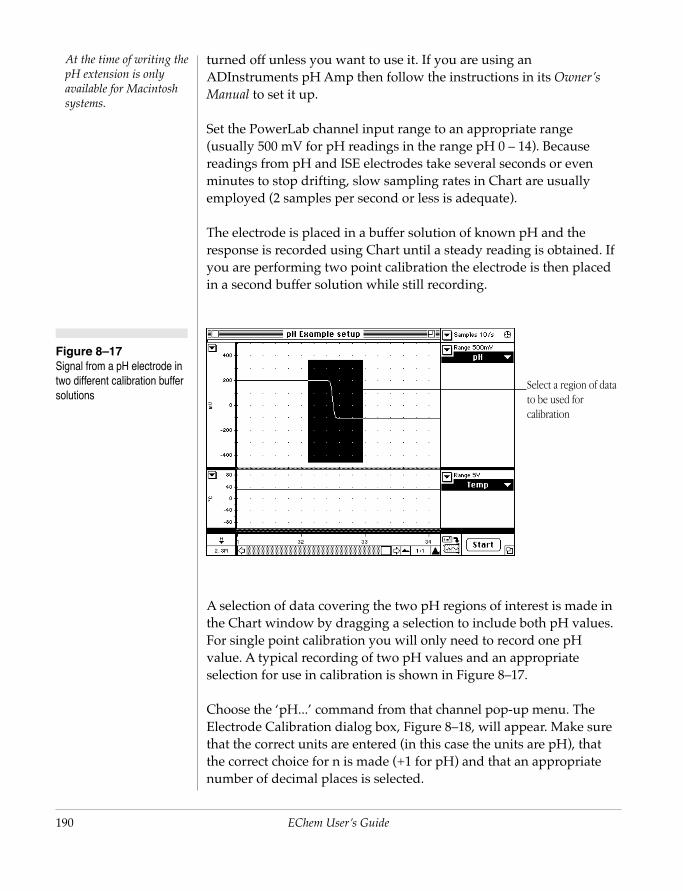
190
Figure 8–17 Signal from a pH electrode in two different calibration buffer solutions
At the time of writing the pH extension is only
turned off unless you want to use it. If you are using an ADInstruments pH Amp then follow the instructions in its Owner’s Manual to set it up.
Set the PowerLab channel input range to an appropriate range (usually 500 mV for pH readings in the range pH 0 – 14). Because readings from pH and ISE electrodes take several seconds or even minutes to stop drifting, slow sampling rates in Chart are usually employed (2 samples per second or less is adequate).
The electrode is placed in a buffer solution of known pH and the response is recorded using Chart until a steady reading is obtained. If you are performing two point calibration the electrode is then placed in a second buffer solution while still recording.
Select a region of data to be used for calibration
available for Macintosh systems.
EChem User’s Guide
A selection of data covering the two pH regions of interest is made in the Chart window by dragging a selection to include both pH values. For single point calibration you will only need to record one pH value. A typical recording of two pH values and an appropriate selection for use in calibration is shown in Figure 8–17.
Choose the ‘pH...’ command from that channel pop-up menu. The Electrode Calibration dialog box, Figure 8–18, will appear. Make sure that the correct units are entered (in this case the units are pH), that the correct choice for n is made (+1 for pH) and that an appropriate number of decimal places is selected.
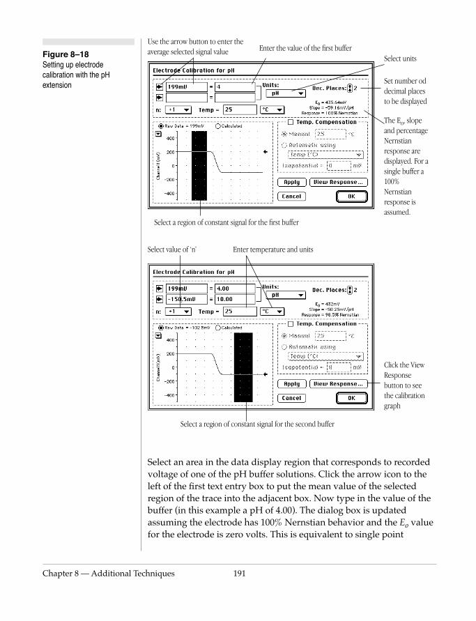
Chapter 8 — Additional Te
Figure 8–18 Setting up electrode calibration with the pH extension
Select a region of constant signal for the first buffer
Use the arrow button to enter the average selected signal value Enter the value of the first buffer
Select units
Set number od decimal places to be displayed
The Eo, slope and percentage Nernstian response are displayed. For a single buffer a 100% Nernstian response is assumed.
Click the View Response button to see the calibration
Enter temperature and unitsSelect value of ‘n’
chniques 191
Select an area in the data display region that corresponds to recorded voltage of one of the pH buffer solutions. Click the arrow icon to the left of the first text entry box to put the mean value of the selected region of the trace into the adjacent box. Now type in the value of the buffer (in this example a pH of 4.00). The dialog box is updated assuming the electrode has 100% Nernstian behavior and the Eo value for the electrode is zero volts. This is equivalent to single point
Select a region of constant signal for the second buffer
graph

192
calibration. An example of this process is shown in the top dialog in Figure 8–18.
Next select a region of the trace in the data display area which represents the value of the second buffer. You only need to do this if you are performing a two point calibration. Click the arrow button to the left of the second row of boxes to enter the mean value into the second entry box. Type in the value of the second buffer (pH 10.00). The slope, Eo value, and percentage Nernstian response of the electrode is then calculated and displayed. An example of this process is shown in the bottom dialog in Figure 8–18.
The calibration data entered will only be applied to the raw millivolt data in the Chart window when the OK or Apply button is clicked. Note that this calibration will be applied to all data in the channel, whether it is pH (or pNa, pCl etc.) data or not. It is therefore important to remember to use one electrode per channel per data file.
The pH calibration can be turned off at any time by choosing the No Calculation command from the channel pop-up menu. This allows you to return to the raw millivolt electrode signal at any time.
Ionic Charge
The n pop-up menu lets you set the value for the number of electrons transferred at the electrode. This usually corresponds to the charge of the ion be measured. You can choose a value between ±3. For pH measurements this value should be set to +1. The value of n is used internally to calculate the response of the electrode using the Nernst equation.
EChem User’s Guide
Calibration Temperature
The temperature of the solutions used for calibration is entered in this text box. Units of Celsius, Kelvin or Fahrenheit can be selected. The buffer solutions you use should have accurately known values at the temperature at which the calibration is performed.
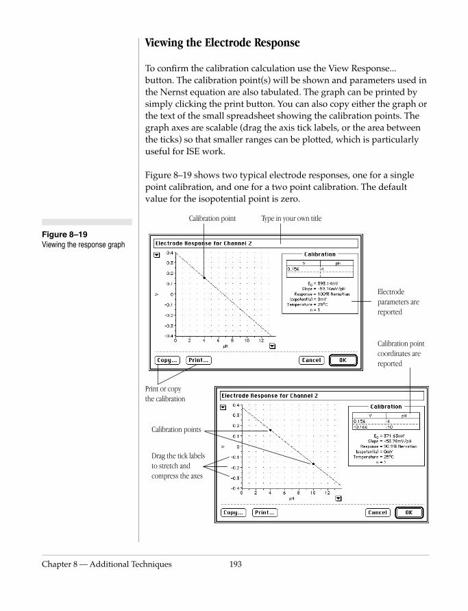
Chapter 8 — Additional Te
Figure 8–19 Viewing the response graph
Viewing the Electrode Response
To confirm the calibration calculation use the View Response... button. The calibration point(s) will be shown and parameters used in the Nernst equation are also tabulated. The graph can be printed by simply clicking the print button. You can also copy either the graph or the text of the small spreadsheet showing the calibration points. The graph axes are scalable (drag the axis tick labels, or the area between the ticks) so that smaller ranges can be plotted, which is particularly useful for ISE work.
Figure 8–19 shows two typical electrode responses, one for a single point calibration, and one for a two point calibration. The default value for the isopotential point is zero.
Calibration point
Print or copy
Electrode parameters are reported
Calibration point coordinates are reported
Type in your own title
chniques 193
Calibration points
the calibration
Drag the tick labels to stretch and compress the axes

194
The vertical axis of the plot will be automatically scaled to the full scale range that the data was recorded at. So, for instance, if you were recording on the 500 mV range then the scale would have a range of ± 500 mV. If the response does not go anywhere near the current full scale range you can drag or stretch the vertical axis to obtain a more detailed plot.
The horizontal axis represents the ionic concentration and is by default pH. In the case of pH the horizontal scale will be automatically scaled to be between 0 and 14 pH. This scale can also be dragged or stretched to view the response plot in more detail. The small arrow pop-up menu next to the horizontal axis allows you to use the set scale feature to adjust the axis between two values.
The electrode response dialog can be copied to the Clipboard for export to a word processor or another application or can be printed for a permanent record. The title area at the top of the dialog is editable so that an electrode serial number or other information can be entered instead of the default title.
Temperature Compensation
There will be times when pH or other ISE measurements will be made at temperatures other than the temperature under which calibration was performed. The greater the change in temperature from the calibration temperature the greater the error in the electrode reading. Also the further away from the isopotential point the greater the error. To overcome this problem most pH meters provide a method for temperature compensation using the Nernst equation as a
EChem User’s Guide
basis for compensation.
The pH extension offers both Manual and Automatic Temperature Compensation (MTC and ATC). Both MTC and ATC corrections can be turned off so you can return to the uncompensated data.
Manual Temperature Compensation (MTC)
The MTC option is for use when you need to make your measurements at a temperature other than that at which the electrode was calibrated. For instance the calibration may have taken place at 25°C but you need to record a solution that will be at 65°C. MTC will
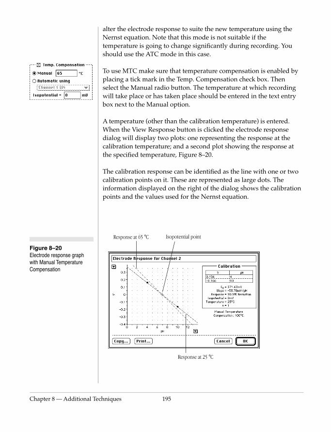
Chapter 8 — Additional Te
Figure 8–20 Electrode response graph with Manual Temperature Compensation
alter the electrode response to suite the new temperature using the Nernst equation. Note that this mode is not suitable if the temperature is going to change significantly during recording. You should use the ATC mode in this case.
To use MTC make sure that temperature compensation is enabled by placing a tick mark in the Temp. Compensation check box. Then select the Manual radio button. The temperature at which recording will take place or has taken place should be entered in the text entry box next to the Manual option.
A temperature (other than the calibration temperature) is entered. When the View Response button is clicked the electrode response dialog will display two plots: one representing the response at the calibration temperature; and a second plot showing the response at the specified temperature, Figure 8–20.
The calibration response can be identified as the line with one or two calibration points on it. These are represented as large dots. The information displayed on the right of the dialog shows the calibration points and the values used for the Nernst equation.
Response at 65 °C Isopotential point
chniques 195
Response at 25 °C

196
Figure 8–21 Warning dialog if Automatic Temperature Compensation is attempted without first setting up a temperature channel
Automatic Temperature Compensation (ATC)
There may be circumstances where the temperature of the solution being measured cannot be maintained at a constant temperature. In this case the pH extension provides the necessary functionality to perform real-time, or automatic, temperature compensation.
Using the Temperature amplifier of the pH Amp, or a temperature signal from a third party temperature measurement device, the temperature signal can be recorded on a second PowerLab channel. When the Automatic option is chosen, the pH extension will use temperature data from one of the Chart channels to correct the pH channel for variations in temperature. To choose the automatic temperature compensation option click in the radio button next to the Automatic option. The channel selection pop-up menu will no longer be grayed out and you can choose the channel on which temperature was recorded.
Recording Temperature for ATC
To record and use a temperature channel with the ATC, the channel must be appropriately calibrated using the Units Conversion feature. The units must be set to either °C, °F, or K. If you have not calibrated the temperature channel you will be warned by the dialog box shown in Figure 3–7. This is necessary because the pH extension will look at the units first to determine the conversion factor required the Nernst equation.
EChem User’s Guide
Isopotential Point
The isopotential point of the electrode is that potential which remains constant as the temperature changes. Most pH electrodes are constructed so that the isopotential point is about 0 mV (which for most pH electrodes also corresponds to pH 7). But it is usual, even in

Chapter 8 — Additional Te
new pH electrodes, that the isopotential point is actually anywhere between ±50 mV and that this value changes as the electrode ages.
Ion selective electrodes may have an isopotential completely outside the measuring range of the electrode.
Most pH meters assume an isopotential point of 0 mV (at pH 7) and then apply either manual or automatic temperature compensation. The Chart pH extension however allows you to set the isopotential point to an appropriate value. To calculate the isopotential point, two calibration runs must be made at two different temperatures, T1 and T2.
From the Nernst equation:
E = E01 + (slope1) pH or pH = (E – E01)/slope1E = E02 + (slope2) pH or pH = (E – E02)/slope2
where
slope1 = –RT1/nF and slope2 = –RT2/nF
At the isopotential point both potential and pH are constant for both T1 and T2, that is E = Eip, and pH = pHip. From the above equations we derive:
which can be solved for Eip:
Eip E01–( )
slope1---------------------------
Eip E02–( )
slope2---------------------------=
Eip
E01 E02–( )
slope1 slope2–---------------------------------------=
chniques 197
or:
For best results ensure that T1 and T2 are at least 20 degrees apart.
Potentiometric TitrimetryThe ADInstruments µPump, can be used to deliver 50 µL aliquots of titrant to a vessel with a coefficient of variability of 0.3%. It is suitable
Eip
E01 E02–( )nF
R T1 T2–( )-----------------------------------=

198
(after calibration) for performing titrations on a scale similar to that used with a conventional 25 or 50 mL burette. Monitoring such a titration is best achieved with Chart software, plotting volume and current flow on separate channels. Chart also has the ability to perform XY plots so that current can be plotted against volume of titrant added.
Dissolved Oxygen, dO2, SensorsUsually the sensor electrode and meter will be purchased from the same manufacturer because the gain settings of the meter must be appropriate for the current signal from the electrode. The recorder output of the dO2 meter can be connected to your PowerLab unit. On line measurements can be made over periods of less than a second to weeks if need be. This can be an ideal way to monitor water quality over a long period of time, or for monitoring of fermentation reactors.
Most oxygen sensors exhibit a slow response time and will take at least 20 s to stabilize. The Units Conversion feature of Chart can be used to perform two point calibration of the signal which is satisfactory for most uses. If multiple point or non-linear calibration is required then the Chart ‘MPCalibration extension’ can be used. See Application Note AN112 (downloadable in Adobe Acrobat® ‘pdf’ format from http://www.adinstruments.com).
Conductivity SensorsConductivity measurements are usually performed with a pair of
EChem User’s Guide
platinum plate electrodes. The conductivity meter provides a small amplitude AC signal from 50 – 1000 Hz (to prevent hydrolysis of the solution) and should provide a recorder type signal that is proportional to the conductivity of the solution. The Units Conversion feature of Chart can be used to perform two point calibration of the signal which is satisfactory for most uses. If multiple point or non-linear calibration is required then the Chart ‘MPCalibration extension’ can be used. See Application Note AN112 (downloadable in Adobe Acrobat® ‘pdf’ format from http://www.adinstruments.com)
Chapter 8 — Additional Te
WARNINGThe connection of multiple Galvanic cells in series can lead to the production of dangerous voltages. PowerLab units are designed to accept voltages up to ±10V. Physical damage to the units will occur if the voltage exceeds 35V.
Simple Galvanic CellsSimple galvanic cells used in undergraduate and high school experiments, for example a Zn | 1 M ZnSO4 || 1 M CuSO4 | Cu system set up in two beakers joined by a salt bridge can be connected by wiring the electrodes (anode and cathode) directly to the PowerLab inputs. There are two ways to do this for a galvanic cell:
• connect one electrode to the centre wire of a shielded cable with a BNC connector at the other end. The second electrode should be connected to the shield of the cable. The BNC connector of the cable can now be plugged into the Channel 1 (or Channel 2 etc.) of a PowerLab unit.
• connect one electrode to the centre wire of a shielded cable with a BNC connector at the other end, and plug this into Channel 1+ of two or four channel PowerLab unit (these units feature differential inputs). Connect the second electrode to the centre wire of a second cable and plug this into Channel 1– of the PowerLab. Make sure that the + and – checkboxes are both checked in the Input Amplifier window to enable differential input.
The second configuration is the one to be preferred as it allows easy reversal of the polarity of the system and allows maximum shielding of the wiring which may be important where small potentials are being measured.
However, for highest precision work for small potentials, or if your
chniques 199
cell has a high internal resistance, then your electrodes should be connected to a ADInstruments GP Amp (input impedance 108 Ω, ±200 mV maximum), or to a pH meter, or to an ADinstruments pH Amp (±2 V maximum, input impedance 3 × 10¹² Ω), which in turn is connected to the PowerLab. If in doubt always use a pH meter or the ADInstruments pH Amp.

200
Quartz Crystal MicrobalanceThe use of a potentiostat to control the potential of an electrode which is also the sensor of a Quartz Crystal Microbalance (QCM) allows mass changes to be detected during a voltammetric experiment.
You will need a QCM with analog recorder output. A PowerLab (with at least four channels) with Chart software to monitor current, potential and mass signals is also required. If you want to control the potentiostat then a PowerLab/4SP, /8SP, or /16SP is recommended as these units can be configured with Chart software to provide a triangular waveform (sent to the potentiostat for a cyclic voltammetric experiment) while recording on all channels. EChem software can only record current and potential and is not suitable for QCM use.
Electrochemical Noise Experi-mentsPowerLab units with Chart software can be used to measure the current and/or potential signals from potentiostats, galvanostats and potential meters. If you are measuring the noise associated with these signals then you should consult Application Notes AN002 and AN007 which discuss the determination of RMS (root mean square) and Noise (the standard deviation) functions of a signal, and the application of digital filtering of a signal. Also of interest is the Spectrum command in Chart (Windows menu) which can be used for
EChem User’s Guide
frequency (FFT) analysis of the signal. This can be us use in determining if the ‘noise’ seen is actually a high frequency interference. Make sure that you are recording at a rate at least twice as fast as the highest frequency component that you need to detect.
At the time of writing these features are only available on Macintosh systems.
Application notes can be downloaded from our web site at http://www.adinstruments.com.

Chapter 8 — Additional Te
Corrosion MeasurementsEChem can be used to drive a potentiostat to perform simple electrochemical corrosion experiments. Because very slow scan rates are employed make sure that you are running EChem in slower speed mode (100 Hz, 400 Hz, or 1000 Hz) when attempting these experiments or you are likely to encounter warning messages saying that the sampling periods are too long.
In addition PowerLab with Chart and Scope software can be used to monitor potentiostat systems replacing existing XYT plotters and chart recorders. In general Chart will be more useful than Scope for these techniques as the slowest Scope can be run at is 2 Hz for 2560 points, a total of 20 minutes per scan. Chart can be run as slow as 12 points per hour for an indefinite period.
Choice of Potentiostat
The American Society for Testing and Materials (ASTM) has put forward several standard protocols performing corrosion experiments. The ADinstruments’ Potentiostat meets the requirements of ASTM G5–87 for potentiostatic and potentiodynamic polarization measurements ASTM G61–86 for cyclic potentiodynamic polarization measurements, and ASTM G59–91 for polarization resistance measurements. However you should note that this requires that the potentiostat have a maximum current rating of only 100 mA. If you require a potentiostat with greater capability then consult Chapter 9 for a suitable instrument that will be compatible with
chniques 201
PowerLab. Also the ADinstruments Potentiostat provides a signal that is proportional to current. Some third party potentiostats have an option so that a recorder signal proportional to log of the absolute current can be obtained. By using such a potentiostat with EChem, Chart, or Scope, the PowerLab system will be able to present data as log of current versus potential.
See ASTM Designation G15 – 90a for standard terminology relating to corrosion experiments, and also ASTM G3: Practice for Conventions Applicable to Electrochemical Measurements in Corrosion Testing.
For most experiments the value of Ecorr must first be determined by measuring the resting potential of your system. This is usually done
202
by connecting a high impedance digital voltmeter (or pH meter in millivolt mode) across the working and reference electrodes before the potentiostat is connected. You may have to wait a few minutes for the reading to stabilize.
Potentiodynamic Polarization
This is essentially Linear Sweep Voltammetry at very slow scan rates, typically 0.6 V/hour ≈ 0.16667 mV/s, over a potential range that is up to Ecorr ± 500 mV.
The potential range should be limited so that extensive water hydrolysis does not occur as this is likely to produce large currents that may overload the potentiostat, while bubbles on the working electrode may alter the rate and type of corrosion taking place, as well as interrupting current flow and causing a noisy signal. Also the use of larger potentials than necessary may also accelerate corrosion to the extent that the surface of the working electrode is altered sufficiently so that results cannot be reproduced.
This type of scan can also be set up using the Multi Pulse technique. EChem should be run at slower speeds (100 Hz – 1 kHz mode) for these types of experiment to enable longer step widths and data sampling periods to be used.
The output from EChem is displayed as current versus the potential. If you wish to display the results as the log of current density versus potential then the data should be transferred to a third party graphing program, for example IGOR Pro. A set of macros for IGOR
EChem User’s Guide
Pro are available from your ADInstruments dealer to facilitate plotting of the data in this format.
If you are used to performing this type of experiment with analog potentiostats then you may wish to do several comparison runs with known materials to compare results. EChem generates a staircase ramp and samples the current over a fixed period of time at a constant potential then averages the current value at each potential. This may lead to smoother graphs and more reproducible results than you are accustomed to. Make the sampling period a multiple of 20 ms (if you use 50 Hz mains) or 16.7 ms (if you use 60 Hz mains) to eliminate noise due to mains hum.
Chapter 8 — Additional Te
Cyclic Potentiodynamic Polarization
See ASTM Designation G61 – 86 for a description of the standard test method. This experiment can be set up with the Cyclic Voltammetry in EChem using very slow scan rates typically 0.6 V/hour (0.1667 mV/s). EChem should be run at slower speeds (100 Hz – 1 kHz mode) for these types of experiments. If the results need to be plotted as the log of current density versus potential then the data will need to be transferred to a specialist graphing program, or you will need to employ a third party potentiostat with a recorder output proportional to the log of current flow.
If you require more control over the sampling period use the Multi Pulse technique with the Cyclic Parameters setting to define your own forward and reverse scan procedures.
Polarization Resistance
See ASTM Designation G59 – 91 for a description of the standard practice. This experiment is simply Linear Sweep (or Cyclic) Voltammetry over a restricted potential range (usually Ecorr ± 30 mV) at slow scan rates, typically 0.6 V/hour. This can be performed using EChem software after first determining Ecorr with a potentiodynamic polarization scan, or with a high impedance voltmeter.
Make sure that EChem is running in a slower mode (100Hz – 1kHz) when performing these experiments. This technique can also be set up in the Multi Pulse technique. Results are usually plotted as current versus potential.
chniques 203

204
EChem User’s Guide
E
Chem User’s Guide9
C H A P T E R T W E L V EUsing 3rd PartyEquipment
You may wish to use you PowerLab with a potentiostat other than the
ADInstruments Potentiostat. This is necessary for:
• very low current situations; or for
• high current/ high power situations.
• or you may have existing potentiostats in your laboratory that you want to use with a computer.
This chapter takes a look at some of the third party equipment that is
compatible with a PowerLab unit using EChem, Chart, or Scope
software. PowerLab units can also be used with many patch, voltage,
or current clamps such as those made by Axon, Warner, or WPI.
205
Connection of third party potentiostats to your PowerLab unit is
discussed in Chapter 3.
For very low current (picoampere range) work look for the release of
our special low current Picostat (under development at time of
writing).
206
CAUTION Please remember that many of these potentiostats are high power models capable of producing dangerous voltages. They should only be used after reading the manufacturer's instruction manuals and becoming thoroughly acquainted with the hazards.
IntroductionThere is an extensive range of potentiostats manufactured by third parties that are compatible with PowerLab. In most cases all that is required is a simple cable connection to the PowerLab.
A range of adaptor cables can also be purchased from your ADInstruments dealer.
EG&G PARC Many of the potentiostat models made by EG&G Princeton Applied Research (PAR) are suitable for connection to PowerLab systems. A brief summary of the different PAR models that can be connected to PowerLab is given in Table 7–1 at the end of this section. More information can be found at http://www.egginc.com/par.
Model 170 potentiostat
This model has been superseded but if you already own one it can be connected to a PowerLab system using Chart and Scope for plotting, or using EChem to drive the potentiostat and plot the data. The 170 has a very high compliance (100 V) and due caution should be taken in its use. The 170 allows AC polarography/voltammetry. Your electronics workshop can construct a cable to enable EChem to drive the 173, otherwise an MLC–01 Cable Kit can be used to record data with Chart and Scope.
EChem User’s Guide
Model 173 potentiostat
This model has been superseded but if you already own one it can be connected to a PowerLab system using Chart or Scope for plotting, or using EChem to drive the potentiostat and plot the data. The 173 potentiostat has a very high compliance (100 V) and due caution should be taken in its use. Your electronics workshop can construct a cable to enable EChem to drive the 173, otherwise an MLC-01 Cable Kit can be used to record data with Chart and Scope.
Chapter 9 — Using 3rd Par
CAUTIONThe 273 potentiostats have a very high compliance (100 V). Read the manufacturers manual and make sure you observe the correct safety procedures.
Model 174 potentiostat
This model has been superseded but if you already own one it can be connected to a PowerLab system using Chart and Scope for plotting, or using EChem to drive the potentiostat and plot the data. The 174 has a very high compliance and due caution should be taken in it use. If you have a 174/51 dual cell differential operation is possible. The 174/50 configuration allows AC polarography.
Model 175 Universal Programmer
The 175 is essentially a waveform generator capable of outputting pulses or a potential ramp. It can be used to drive potentiostats capable of accepting a waveform input. It would normally be used with a potentiostat and the PowerLab system could be used with Chart or Scope to replace an XY plotter or oscilloscope. The MLC-01 Cable Kit is available to connect your PowerLab to this instrument.
The use of a PowerLab unit as a waveform generator with EChem, Chart or Scope software renders the Model 175 largely redundant but it is still useful if you require true analog ramps.
Models 263, 273, and 273A potentiostats
The 263, and 273 series of potentiostats would normally used with PAR's own programs via their inbuilt GPIB IEEE interfaces and an IBM clone computer. However, they can also be used with a Macintosh computer and a PowerLab. You may prefer to use the potentiostat in its stand alone mode and use the combination of
ty Equipment 207
Scope/Chart and a PowerLab for plotting your data rather than a standard XY plotter, or you can control the potentiostat by generating stepped and pulsed waveforms with EChem. The MLC–01 Cable Kit is available to connect your PowerLab to this instrument.
Model 264A potentiostat
The 264A Polarographic Analyser/Stripping Voltammeter can benefit by using a PowerLab/200 with Scope or Chart in place of its standard XY plotter. Alternatively it can be used with EChem to drive it and replace its inbuilt techniques. The MLC–01 Cable Kit is available from to connect your PowerLab to this instrument.
208
Model 363 potentiostat
The 363 is a non–scanning potentiostat/galvanostat with a maximum current rating of 1 A and 30 V compliance making it ideal for corrosion and plating studies, and electrosynthesis. Combining this potentiostat with a PowerLab/EChem system will enable it to become a scanning instrument. All the techniques offered by EChem will then be available with this potentiostat. Newer models of the 363 have inbuilt positive feedback iR compensation. The MLC–02 Cable Kit is available to connect your PowerLab to this instrument.
Model 362 potentiostat
This model has similar specifications to the 362 potentiostat with the added advantage that it can provide its own analog ramp. This means that techniques that require a true analog ramp can be monitored with a PowerLab controlled with Chart or Scope. The 362 comes equipped with positive feedback iR compensation. The MLC–02 Cable Kit is available to connect your PowerLab to this instrument.
Model 366 Bipotentiostat
Ring /disk work requires a bipotentiostat (or two single potentiostats). The model 366 bipotentiostat can be used with a PowerLab in several ways, including:
• a PowerLab/200 or /400 could be used to drive the ring or disk electrode with EChem (via the external input) while a constant potential is applied to the disk (or ring) with the other half of the
EChem User’s Guide
bipotentiostat. When using EChem only two channels of data can be recorded.
• a PowerLab/400 and Chart could monitor current and potential at the ring as the ring potential is ramped, while simultaneously monitoring current at the disk as it is held at constant potential. A total of three channels of data would be recorded.
For maximum recording flexibility with this instrument a four (or more) channel PowerLab unit is recommend. The MLC–03 Cable Kit is available to connect your PowerLab to this instrument.
Chapter 9 — Using 3rd Par
Model 400 electrochemical detector
The Model 400 electrochemical detector is designed for liquid chromatography. Both outputs on the Model 400 can conveniently be monitored with a PowerLab/200 and Chart. With a PowerLab/400 the signals from two Model 400's could be monitored. The MLC–01 Cable Kit is available to connect your PowerLab to this instrument.
If you are using a Model 400 detector and a UV-visible or fluorescence detector you can monitor the outputs of any two detectors simultaneously with Chart and a PowerLab/200. With a PowerLab/400 you can monitor the output of up to four detectors. Extra virtual channels are provided which can be used for on-line integration of the incoming signals (using the Computed Input feature).
The Model 400 is also suitable for connection to our PowerChrom system which offers many more features suitable for chromatographic data analysis.
Model 303A Static Mercury Drop Electrode
The PAR 303A Static Mercury Drop Electrode (SMDE) can also be used as a Hanging Mercury Drop Electrode or Dropping Mercury Electrode (HMDE or DME). It can be used with a PowerLab/EChem system, either with a third party potentiostat, or with a ADInstruments Potentiostat.
ty Equipment 209

Chapter 9 — Us
Table 10–1 Comparison table fPARC equipment. 1
Mod
el
366
263
Vers
aSta
t17
017
317
427
3 &
273A
264A
400
LC
Det
ecto
r
yes
yes
yes
yes
yes
yes
yes
yes
yes
yes
yes
yes
yes2.
yes
yes
yes
yes
no
yes
yes
yes
yes
noye
sye
sye
sno
0 to
1
V/s
Proc
esso
r c
ontro
lled
Proc
esso
rco
ntro
lled
0.1
mV/
s to 50
0 m
V/s
–0.
1 m
V/s
to
500
mV/
s
Proc
esso
rco
ntro
lled
1 m
V/s
to 1
0 V/
s1
mV/
s to
10
0 m
V/s
yes
yes
yes
yes
yes
yes
yes
yes
no
±2 V
±8 V
±10
V±5
V±5
V±5
V±1
0 V
±10
V±2
V
10 V
20 V
20 V
100
V10
0 V
80 V
100
V10
V10
V
1 µ
A to
1 A
100
nA to
100
mA
1 µ
A to
250
mA
1 nA
to5
A10
0 µ
A to
1 A
20 n
A to
10 m
A10
0 nA
to10
0 m
A3.10
0 nA
to
5 m
A10
0 nA
to
100
µA
none
feed
back
/cu
rrent
in
terru
pt
curre
nt
inte
rrupt
feed
back
feed
back
feed
back
with
/50
optio
n
feed
back
/ cu
rrent
in
terru
pt
none
noneor EG & G
the
man
ufac
ture
r, sp
ecifi
cati
ons
may
cha
nge
at s
hort
not
ice;
2. T
he e
xter
nal i
nput
sho
uld
be
mod
ified
to a
ccep
t DC
sig
nals
as
inst
ruct
ion
man
ual;
3. R
ange
s of
10
A a
nd 1
nA
can
be
sele
cted
if th
e in
stru
men
t is
cont
rolle
d b
y PA
R’s
ow
n so
ftw
are.
ing 3rd Party Equipment 210
Feat
ure
363
362
Pow
erLa
b as
plo
tter
yes
yes
Pow
erLa
b as
w
avef
orm
gen
erat
orye
sye
s
Inbu
ilt s
cann
ing
noye
s
Inbu
ilt s
can
rate
–0.
1 m
V/s
to 5
V/s
Exte
rnal
inpu
tye
sye
s
Volta
ge ra
nge
±10
V±1
0V
Com
plia
nce
30 V
30 V
Cur
rent
rang
es (f
ull
scal
e)1
µA
to1
A1
µA
to
1 A
iR c
ompe
nsat
ion
feed
back
feed
back
Not
es: 1
. The
se s
peci
fica
tion
s sh
ould
be
veri
fied
by
des
crib
ed in
sec
tion
III,
page
s 1
& 2
of t
he P
AR
170
Chapter 9 — Using 3rd Par
CAUTION.Please remember that these potentiostats should only be used after reading the manufacturer's instruction manuals and becoming thoroughly acquainted with any hazards.
BAS EquipmentRefer to Table 9–2 at the end of this section for a table of equipment made by Bioanalytical Systems Inc. (BAS) at its compatibility with PowerLab. Also see http://www.bioanalytical.com/.
Model CV-1B potentiostat
The CV–1B is BAS's most basic unit and is widely used in teaching laboratories. It is greatly enhanced by connecting its recorder outputs to a PowerLab and recording data with Chart or Scope software. It is not suitable for control with EChem. The MLC–06 Cable Kit is available to connect your PowerLab to this instrument.
To set up scan limits, connect the CV–1B to the PowerLab, I output to Channel 1 and E output to Channel 2. Now open the Input Amplifier on Channel 2. Adjust the scan limits of the CV-1B while using the Input Amplifier window to monitor the value of the potential.
Models CV-27 and CV-37 potentiostats
The CV-27 and CV-37 can both be connected to a PowerLab, with Chart and Scope, to replace a conventional XY plotter. These units can also be controlled with EChem and a PowerLab, allowing full use of stepped ramp and pulse techniques. The MLC-06 Cable Kit is available to connect your PowerLab to these instruments.
Model PWR-3 Power Module potentiostat
ty Equipment 211
The PWR-3 Power Module can be used directly with a PowerLab and EChem or Chart or Scope, or you may use it with one of BAS‘s other potentiostats in combination with PowerLab. Remember that this instrument can produce dangerous voltages and should only be used after thoroughly reading its instruction manual. The MLC-06 Cable Kit is available to connect your PowerLab to this instrument.
Low Current Module potentiostat
The BAS Low Current Module is designed to be used with a waveform generator. This module can be directly attached to a
212
PowerLab unit, and with EChem, Chart, or Scope, software you can perform very low current (sub nA) work with microelectrodes. Note that you do not need to purchase a separate potentiostat! Low current work generally requires the use of a Faraday cage and the low current module is designed to be compatible with BAS's C–2 Cell Stand. The MLC–04 Cable Kit is available to connect your PowerLab to this instrument.
Models 100A and 100B potentiostat workstations
The BAS 100A, and 100B are both equipped with analog recorder outputs which can be connected directly to a PowerLab and the data recorded with Chart or Scope. In addition an analog input is provided so that control of the instrument is possible with a Macintosh computer using a PowerLab and EChem. The MLC–06 Cable Kit is available to connect your PowerLab to these instruments.
Model LC-44
The LC–44 electrochemical detector is designed for liquid chromatography. Both generator and detector current outputs can be monitored with a PowerLab/200 and Chart, or the detector outputs from two LC–44's. With a PowerLab/400 the generator and detector currents from two LC–44's could be monitored. The MLC–07 Cable Kit is available to connect your PowerLab to this instrument.
If you are using an LC–44 detector and a UV-visible or fluorescence detector you can monitor the outputs of any two detectors simultaneously with Chart and a PowerLab/200. With a
EChem User’s Guide
PowerLab/400 you can monitor the output of up to four detectors. Extra virtual channels are provided which can be used for on-line integration of the incoming signals (using the Computed Input feature).
Model RDE-1
The BAS Rotating Disk Electrode can be used with most potentiostats. If your potentiostat is being used with a PowerLab/EChem system then you can connect the RDE–1 to the potentiostat and you will be able to drive the RDE–1 with EChem.
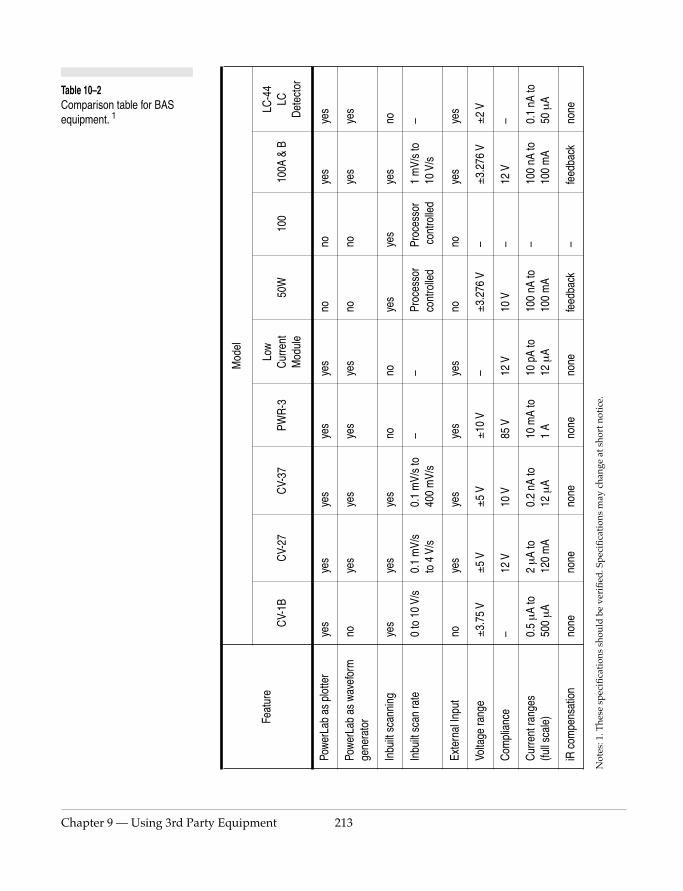
Chapter 9 — Using 3rd
Table 10–2 Comparison table for BAS equipment. 1
Mod
el
CV-
27C
V-37
PWR
-3Lo
w
Cur
rent
M
odul
e50
W10
010
0A &
BLC
-44
LC
Det
ecto
r
yes
yes
yes
yes
nono
yes
yes
yes
yes
yes
yes
nono
yes
yes
yes
yes
nono
yes
yes
yes
no
0.1
mV/
s to
4 V
/s0.
1 m
V/s
to
400
mV/
s–
–Pr
oces
sor
cont
rolle
dPr
oces
sor
con
trolle
d1
mV/
s to
10
V/s
–
yes
yes
yes
yes
nono
yes
yes
±5 V
±5 V
±10
V–
±3.2
76 V
–±3
.276
V±2
V
12 V
10 V
85 V
12 V
10 V
–12
V–
2 µ
A to
12
0 m
A0.
2 nA
to
12 µ
A10
mA
to
1 A
10 p
A to
12
µA
100
nA to
10
0 m
A–
100
nA to
10
0 m
A0.
1 nA
to
50 µ
A
none
none
none
none
feed
back
–fe
edba
ckno
ne
. Spe
cific
atio
ns m
ay c
hang
e at
sho
rt n
otic
e.
Party Equipment 213
Feat
ure
CV-
1B
Pow
erLa
b as
plo
tter
yes
Pow
erLa
b as
wav
efor
m
gene
rato
rno
Inbu
ilt s
cann
ing
yes
Inbu
ilt s
can
rate
0 to
10
V/s
Exte
rnal
Inpu
tno
Volta
ge ra
nge
±3.7
5 V
Com
plia
nce
–
Cur
rent
rang
es
(full
scal
e)0.
5 µ
A to
50
0 µ
A
iR c
ompe
nsat
ion
none
Not
es: 1
. The
se s
peci
ficat
ions
sho
uld
be
veri
fied
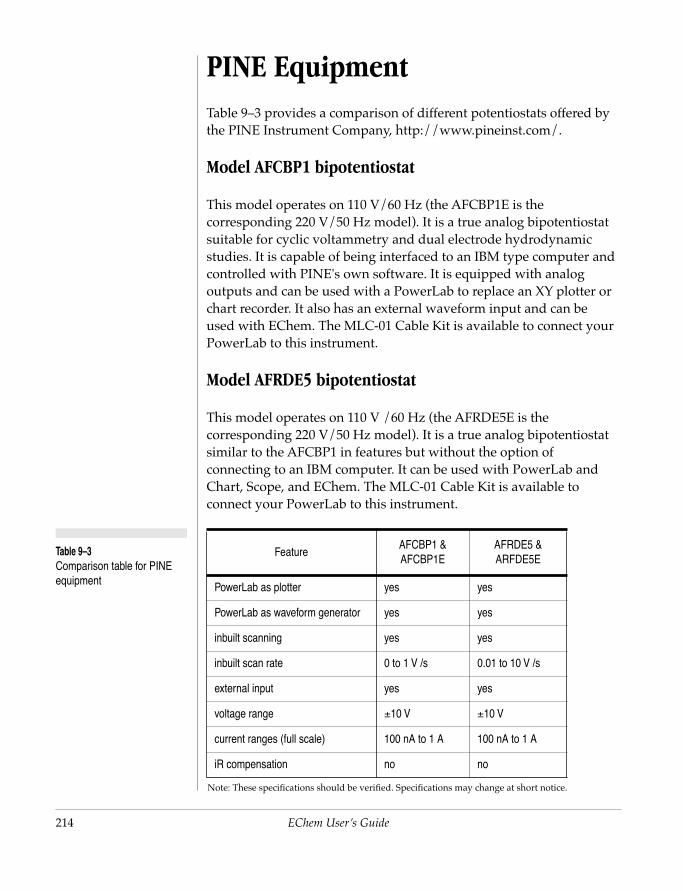
214
Table 9–3 Comparison table for PINE equipment
PINE EquipmentTable 9–3 provides a comparison of different potentiostats offered by the PINE Instrument Company, http://www.pineinst.com/.
Model AFCBP1 bipotentiostat
This model operates on 110 V/60 Hz (the AFCBP1E is the corresponding 220 V/50 Hz model). It is a true analog bipotentiostat suitable for cyclic voltammetry and dual electrode hydrodynamic studies. It is capable of being interfaced to an IBM type computer and controlled with PINE's own software. It is equipped with analog outputs and can be used with a PowerLab to replace an XY plotter or chart recorder. It also has an external waveform input and can be used with EChem. The MLC-01 Cable Kit is available to connect your PowerLab to this instrument.
Model AFRDE5 bipotentiostat
This model operates on 110 V /60 Hz (the AFRDE5E is the corresponding 220 V/50 Hz model). It is a true analog bipotentiostat similar to the AFCBP1 in features but without the option of connecting to an IBM computer. It can be used with PowerLab and Chart, Scope, and EChem. The MLC-01 Cable Kit is available to connect your PowerLab to this instrument.
FeatureAFCBP1 & AFCBP1E
AFRDE5 & ARFDE5E
EChem User’s Guide
PowerLab as plotter yes yes
PowerLab as waveform generator yes yes
inbuilt scanning yes yes
inbuilt scan rate 0 to 1 V /s 0.01 to 10 V /s
external input yes yes
voltage range ±10 V ±10 V
current ranges (full scale) 100 nA to 1 A 100 nA to 1 A
iR compensation no no
Note: These specifications should be verified. Specifications may change at short notice.
Chapter 9 — Using 3rd Par
CAUTIONSome of these combinations have compliance voltages up to 90 V and are a shock hazard. They should be used only after thoroughly reading the instruction manual and being thoroughly acquainted with the possible hazards.
While many experiments can be performed with a PowerLab/200, for maximum flexibility these PINE bipotentiostats should be used with a PowerLab/400. PINE also makes a variety of rotators, and disk and ring disk electrodes. these are also compatible for use with PowerLab systems.
Metrohm EquipmentModel 506 Polarecord with 663 VA Stand
The Metrohm 506 Polarecord™ is found in many analytical laboratories using polarography for trace analysis. It has provision for attachment to an external XY recorder and so Scope or Chart can be used with PowerLab to record data directly to a Macintosh.
It is also possible to use EChem to drive a Polarecord but the pilot voltage connection on the Polarecord has an attenuation of 1:10. Thus the maximum potential range that EChem is capable of (±5 V) will be interpreted as ±0.5 V. To overcome this you can use a 1:10 amplifier to boost the signal before feeding it into the Polarecord, or, if your experiment can be run in a ±0.5 V range, put up with the X-axis being out by a factor of 10.
Model 690 Ion Chromatograph
ty Equipment 215
The Metrohm 690 is a conductivity detector system for ion chromatography. It is ideal for use with PowerLab and Chart to replace a conventional strip chart recorder. The program Peaks can then be used to analyse the data and extract peak heights and areas.
For more advanced chromatography our PowerChrom system is available.
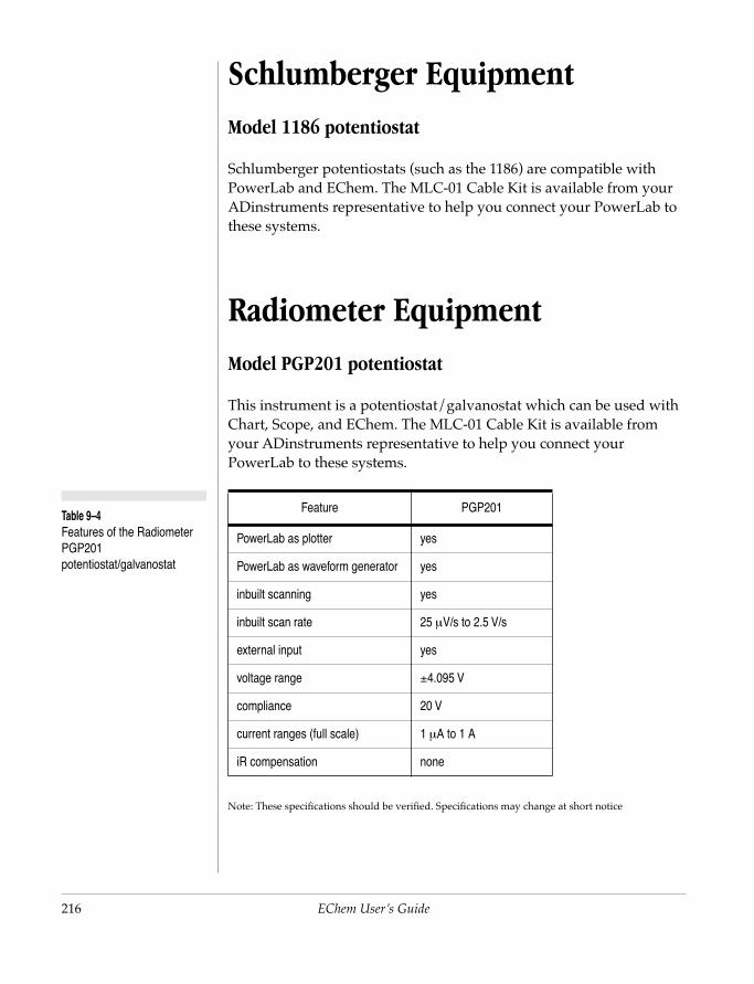
216
Table 9–4 Features of the Radiometer PGP201 potentiostat/galvanostat
Schlumberger EquipmentModel 1186 potentiostat
Schlumberger potentiostats (such as the 1186) are compatible with PowerLab and EChem. The MLC-01 Cable Kit is available from your ADinstruments representative to help you connect your PowerLab to these systems.
Radiometer EquipmentModel PGP201 potentiostat
This instrument is a potentiostat/galvanostat which can be used with Chart, Scope, and EChem. The MLC-01 Cable Kit is available from your ADinstruments representative to help you connect your PowerLab to these systems.
Feature PGP201
PowerLab as plotter yes
PowerLab as waveform generator yes
inbuilt scanning yes
inbuilt scan rate 25 µV/s to 2.5 V/s
EChem User’s Guide
Note: These specifications should be verified. Specifications may change at short notice
external input yes
voltage range ±4.095 V
compliance 20 V
current ranges (full scale) 1 µA to 1 A
iR compensation none

Chapter 9 — Using 3rd Par
Feature
PowerLab as plotter
PowerLab as waveform generator
Inbuilt scanning
Inbuilt scan rate
External Input
Voltage Range
Current Ranges (full scale)
iR Compensation
Note: These specifications sh
Table 9–5 Features of HEKA potentiostats
HEKA EquipmentModels PG28.. series potentiostats
The HEKA™ potentiostats in the PG28 system are all compatible with PowerLab and Chart and Scope for data collection. In addition they can also be used with a PowerLab and EChem so that you can use them as part of a computer controlled system. The MLC-01 Cable Kit is available from your ADinstruments representative to help you connect your PowerLab to these Heka systems.
The basic system comprises modules from the series 100 control amplifiers and the series 200 current amplifiers. In addition the 300 series modules, trigger pulse and scan generators; 400 series modules, current integrators; and 500 series module, digital display; can also be added. Consult http://www.heka.com/ more details.
.
PG28 PG28../5A PG28.B PG284 PG285 PG287
yes yes yes yes yes yes
yes yes yes yes yes yes
ty Equipment 217
no no no yes yes yes
– – – 1 mV/s to 1 kV/s
1 mV/s to 1 kV/s
1 mV/s to 1 kV/s
yes yes yes yes yes no
±10 V ±5 V ±2 V ±10 V ±90 V ±10 V
1 µA to 2 A
1 µA to 2 A
1 µA to 200 mA
1 µA to 1 A
1 µA to 1 A
1 µA to 1 A
feedback feedback feedback feedback feedback feedback
ould be verified. Specifications may change at short notice.
218
Cypress Systems EquipmentCypress Systems make a variety of potentiostats and related information. Latest information can be found at http://www.cypresshome.com/.
Omni 90 Potentiostat
The Omni 90 is a simple potentiostat with inbuilt analog scanning and also able to accept an external input. It can be used with PowerLab replacing the XY plotter or chart recorder with Scope and Chart software, or can be used with EChem software so that stepped ramp and pulse voltammetry can be performed. The MLC-01 Cable Kit is available to connect your PowerLab to this instrument.
Omni 101 Potentiostat
The Omni 101 is a stand alone microprocessor controlled analog potentiostat with inbuilt analog scanning and also able to accept an external input. It can be used with PowerLab replacing the XY plotter or chart recorder with Scope and Chart software, or can be used with EChem software so that stepped ramp and pulse voltammetry can be performed. The MLC-01 Cable Kit is available to connect your PowerLab to this instrument.
CS 1000 Galvanostat/Coulometer
The CS1000 can be used with PowerLab replacing the chart recorder
EChem User’s Guide
with Chart software.
EI 400 Bipotentiostat
The EI 400 is an analog bipotentiostat (which can also be used as a single potentiostat) with inbuilt analog scanning and also able to accept an external input. It can be used with PowerLab replacing the XY plotter or chart recorder with Scope and Chart software, or can be used with EChem software so that stepped ramp and pulse voltammetry can be performed. It is also suitable for use with microelectrodes.

Chapter 9 — Using 3rd Par
Table 9–6 Features of Cypress Systems instruments.
Feature
PowerLab as plotter
PowerLab as waveformgenerator
Inbuilt scanning
Inbuilt scan rate
External Input
Voltage range
Compliance
Current ranges
iR Compensation
Note: These specifications s
Model
Omni 90 Omni 101 CS 1000 EI 400
yes yes yes yes
yes yes no yes
yes yes no yes
– <100 mV/s to 1000 V/s
yes yes no yes
±2.5 V ±2 V ±10 V
10 V 15 V 18 V 10 V
0.01µA to 100mA 100nA/V to 100mA/V
100 µA/V to 1 A 100 pA/V to 100 nA/V
no no no no
hould be verified. Specifications may change at short notice.
ty Equipment 219
220
AMEL EquipmentLatest information on AMEL potentiostats can be found at http://www.amelsrl.com/.
Model 2049 Potentiostat
The 2049 has an external input and can be used with PowerLab replacing the XY plotter or chart recorder with Scope and Chart software, or can be used with EChem software so that stepped ramp and pulse voltammetry can be performed. The MLC-01 Cable Kit is available to connect your PowerLab to this instrument.
Model 2051 Potentiostat/Galvanostat
The 2051 has an external input and can be used with PowerLab replacing the XY plotter or chart recorder with Scope and Chart software, or can be used with EChem software so that stepped ramp and pulse voltammetry can be performed. The MLC-01 Cable Kit is available to connect your PowerLab to this instrument.
Model 2053 Potentiostat/Galvanostat
The 2053 has an external input and can be used with PowerLab replacing the XY plotter or chart recorder with Scope and Chart software, or can be used with EChem software so that stepped ramp and pulse voltammetry can be performed. The MLC-01 Cable Kit is available to connect your PowerLab to this instrument.
EChem User’s Guide
Model 2053 High Current Potentiostat
The Omni 101 is a high current (up to 12 A) potentiostat/galvanostst able to accept an external input. It can be used with PowerLab replacing the XY plotter or chart recorder with Scope and Chart software, or can be used with EChem software so that stepped ramp and pulse voltammetry can be performed. The MLC-01 Cable Kit is available to connect your PowerLab to this instrument.

Chapter 9 — Using 3rd Par
Table 9–7 Features of AMEL instruments.
Feature
PowerLab as plotter
PowerLab as waveformgenerator
Inbuilt scanning
External Input
Voltage range
Compliance
Current ranges
iR Compensation
Note: These specifications sho
Model
2049 2051 2053 2055
yes yes yes yes
yes yes yes yes
no no no no
yes yes yes yes
±5 V ±5 V ±5 ±5 V
22 V 27 V 50 V 30 V
1µA to 1 A 1µA to 1 A 1µA to 1 A 100 µA to 10 A
no no yes no
uld be verified. Specifications may change at short notice.
ty Equipment 221

222
EChem User’s Guide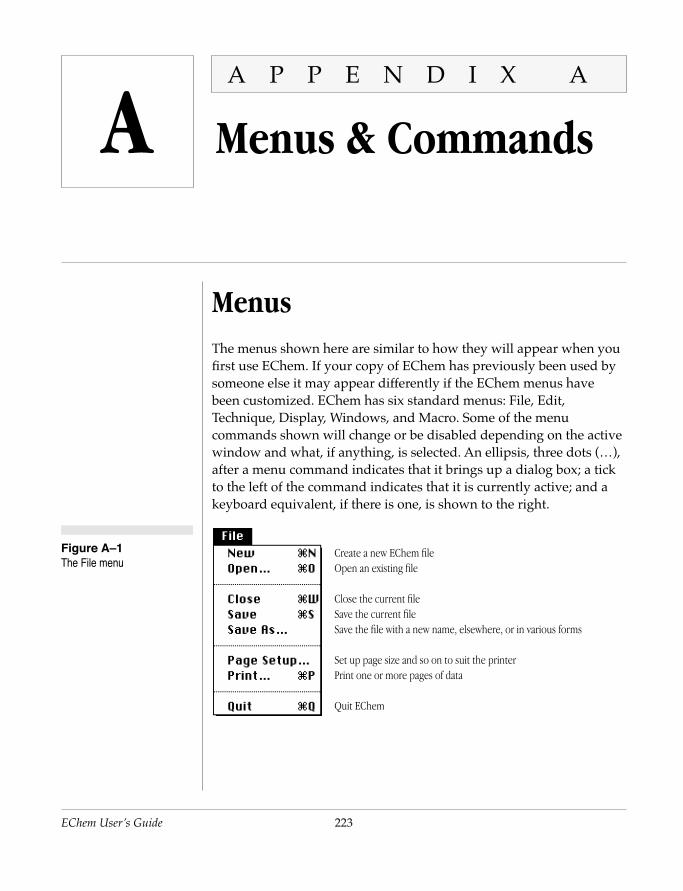
EChem
FigurThe Fil
User’s Guide
A
e A–1 e menu
A P P E N D I X A
Menus & Commands
MenusThe menus shown here are similar to how they will appear when you
223
first use EChem. If your copy of EChem has previously been used by someone else it may appear differently if the EChem menus have been customized. EChem has six standard menus: File, Edit, Technique, Display, Windows, and Macro. Some of the menu commands shown will change or be disabled depending on the active window and what, if anything, is selected. An ellipsis, three dots (…), after a menu command indicates that it brings up a dialog box; a tick to the left of the command indicates that it is currently active; and a keyboard equivalent, if there is one, is shown to the right.
Create a new EChem fileOpen an existing file
Close the current fileSave the current fileSave the file with a new name, elsewhere, or in various forms
Set up page size and so on to suit the printerPrint one or more pages of data
Quit EChem
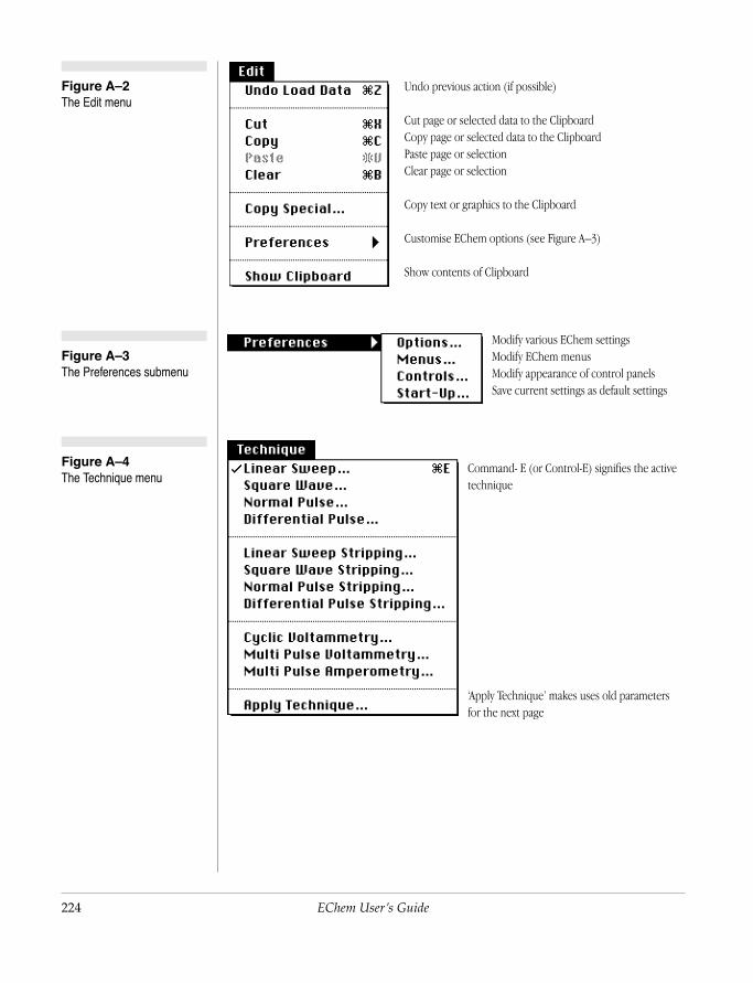
Undo previous action (if possible)
Cut page or selected data to the ClipboardCopy page or selected data to the Clipboard
Figure A–2 The Edit menu
Paste page or selectionClear page or selection
Copy text or graphics to the Clipboard
Customise EChem options (see Figure A–3)
224 EChem User’s Guide
Figure A–3 The Preferences submenu
Figure A–4 The Technique menu
Show contents of Clipboard
Modify various EChem settingsModify EChem menusModify appearance of control panelsSave current settings as default settings
Command- E (or Control-E) signifies the active technique
‘Apply Technique’ makes uses old parameters for the next page

Modify display colours, grids, lines, and so onGo to a particular page of a file quickly
Figure A–5 The Display menu
Show or hide an overlaid pageTurns all overlays onTurns all overlays offModify the way overlaid waveforms are displayed
Sets the current sampling display method
Keep selected background but don’t subtractSelect a scan to be backgroundDeselect background scan
Figure A–6 The Windows menu
Display Notebook window. Write general notes on the file
Return to, or open the main EChem windowDisplay a selection in the Zoom window
Define selection areaDefine marker position
Bring up Data Pad windowLog results to Data Pad
Appendix A — Menus & Commands 225
Figure A–7 The Macro menu
Figure A–8 The Macro Commands submenu. The Speak Message and AppleScript commands are available only on Macintosh systems.
Start or stop recording a macroDelete a macro from the current list of macros
Choose macro control actions (see Figure A–8)
Pause the macro for a set timeSet an audible alert using the System sounds
Display a message dialog box (requiring user action)Speak a written message (if the computer can do this)
Add an AppleScript as a macro step
Select each page of data to perform some action toStart a repeat sequence
Finish a repeat sequence
Redraw the screen during the playing of a macro
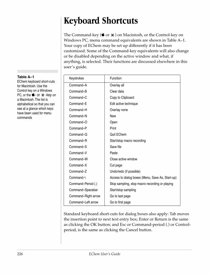
226
Table A–1 EChem keyboard short-cuts for Macintosh. Use the Control key on a Windows PC, or the - or -key on a Macintosh. The list is alphabetical so that you can see at a glance which keys have been used for menu commands
Keyboard ShortcutsThe Command-key ( or ) on Macintosh, or the Control-key on Windows PC, menu command equivalents are shown in Table A–1. Your copy of EChem may be set up differently if it has been customized. Some of the Command-key equivalents will also change or be disabled depending on the active window and what, if anything, is selected. Their functions are discussed elsewhere in this user’s guide.
Keystrokes Function
Command–A Overlay all
Command–B Clear data
Command–C Copy to Clipboard
Command–E Edit active technique
Command–H Overlay none
Command–N New
Command–O Open
Command–P Print
Command–Q Quit EChem
Command–R Start/stop macro recording
Command–S Save file
Command–V Paste
Command–W Close active window
Command–X Cut page
Command–Z Undo/redo (if possible)
EChem User’s Guide
Standard keyboard short-cuts for dialog boxes also apply: Tab moves the insertion point to next text entry box; Enter or Return is the same as clicking the OK button; and Esc or Command-period (.) or Control-period, is the same as clicking the Cancel button.
Command–\ Access to dialog boxes (Menu, Save As, Start-up)
Command–Period (.) Stop sampling, stop macro recording or playing
Command–Spacebar Start/stop sampling
Command–Right arrow Go to last page
Command–Left arrow Go to first page

EChem
FigurThe Ab
User’s Guide
B
e B–1 out EChem dialog box
A P P E N D I X B
Troubleshooting
Technical SupportEChem has been extensively tested to make sure that it runs smoothly and without difficulties. Occasionally, however, problems may arise or something unexpected may occur. The second part of this appendix gives a list of possible problems and likely solutions: you should look there first to see if your needs are addressed specifically.
If you are experiencing difficulties with EChem that are not covered in this user’s guide, or you need technical assistance with your system, then ADInstruments and its authorised distributors are glad to help. The About EChem dialog box provides dealer and distributor addresses and the required system configuration information. To access this information, select the About EChem… command from the Apple () menu on a Macintosh, or go to the Help menu on a Windows computer (click the dialog box when you have finished to
227
make it go away).
Release date
Click this button for information on hardware configuration
Click this button for information on dealer contacts

228
Figure B–2 The ADInstruments Distributor Addresses dialog box
Dealer and Distributor Information
If you need help or information from an authorised PowerLab distributor, click the Telephone button, Figure B–1, to bring up the PowerLab Dealer and Distributor Addresses dialog box. Click in the scrolling list on the right of the dialog box to select your country, or the nearest one to it, and contact information will appear to the left. Feel free to contact your PowerLab dealer to discuss hardware and software requirements generally, and find out more about the latest releases, upgrades, and software maintenance information.
System Configuration Information
In general, you will need to provide specific information about your hardware and software to help to isolate and to solve problems effectively. Since this type of information can be tedious to collate, EChem does it all for you. Click the computer icon-shaped button, Figure B–1,to activate the About This Computer dialog box. There will be a short delay while it gleans the required information from
EChem User’s Guide
your system.
The dialog box gives information on which version of EChem is running, together with a list of system extensions and ‘inits’. Also provided is a detailed description of your Macintosh, your PowerLab and how it is connected, special hardware configurations, and other peripheral devices connected to the computer.
Click the Print button to print the picture (it brings up the Print dialog box), or the Copy to Clipboard button to copy the picture for pasting into a letter or fax to your PowerLab dealer.
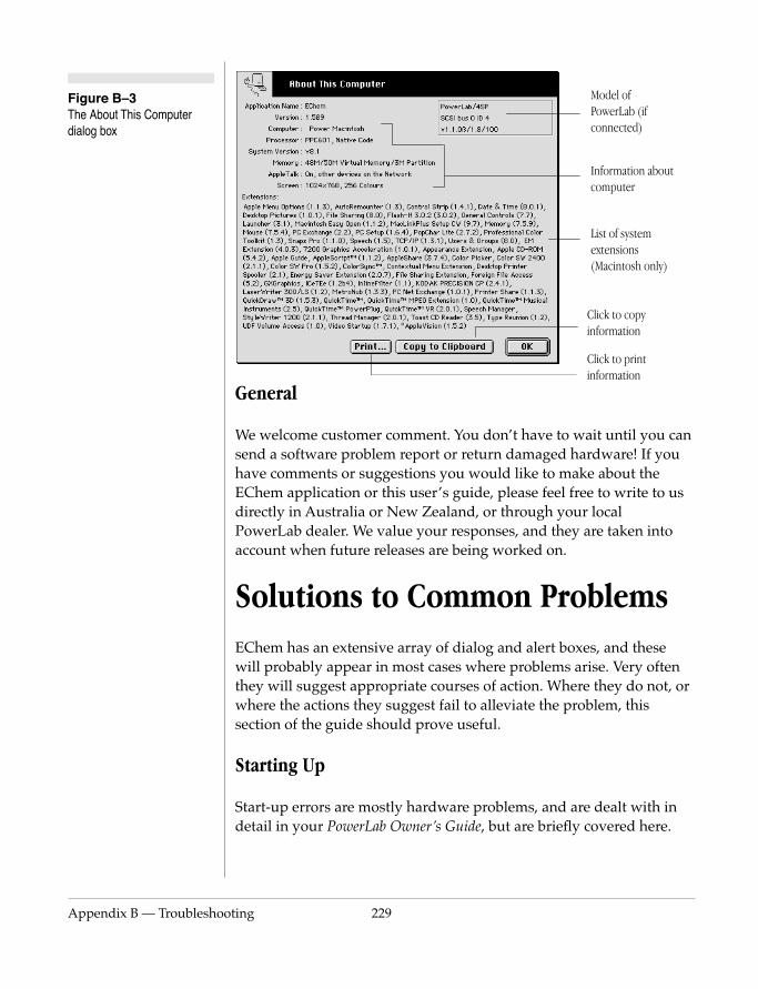
Appendix B — Troublesho
Figure B–3 The About This Computer dialog box
General
We welcome customer comment. You don’t have to wait until you can send a software problem report or return damaged hardware! If you have comments or suggestions you would like to make about the EChem application or this user’s guide, please feel free to write to us directly in Australia or New Zealand, or through your local PowerLab dealer. We value your responses, and they are taken into account when future releases are being worked on.
Solutions to Common Problems
Click to print information
Model of PowerLab (if connected)
Click to copy information
List of system extensions (Macintosh only)
Information about computer
oting 229
EChem has an extensive array of dialog and alert boxes, and these will probably appear in most cases where problems arise. Very often they will suggest appropriate courses of action. Where they do not, or where the actions they suggest fail to alleviate the problem, this section of the guide should prove useful.
Starting Up
Start-up errors are mostly hardware problems, and are dealt with in detail in your PowerLab Owner’s Guide, but are briefly covered here.

230
The computer can’t find the PowerLab unit
The PowerLab is off or the power is switched off at the wall, the power cable is not connected firmly, or a fuse has blown.
• Check switches, power connections, and fuses.
Poor cable connection between the PowerLab and the computer, or a bad cable.
• Ensure that the cable is firmly attached at both ends and try again. If there is still a problem, try a new cable.
The PowerLab has an internal problem or has ‘hung’
• Turn off the computer and PowerLab (and any other devices in the SCSI chain), and then turn the PowerLab back on again after at least ten seconds. Turn on the computer and try using EChem again.
SCSI problems: two SCSI devices on the bus have the same SCSI ID, or termination is incorrect.
• Check that each device has a unique ID number and that the SCSI chain is terminated correctly.
EChem ‘hangs’ or gives an alert on start-up
SCSI problems: two SCSI devices on the bus have the same SCSI ID, or termination is incorrect.
EChem User’s Guide
• Check that each device has a unique ID number and that the SCSI chain is terminated correctly.
It may be that the application has become damaged in some way.
• Try reinstalling EChem from the original CD
EChem starts up with strange settings and macros
You started EChem by opening a data file with custom settings or a settings file, or the start-up settings have been customised.
Appendix B — Troublesho
• Start up again from the application itself. To start up EChem with its default settings, hold down the Command key as you open the application (straight after double-clicking it). Release the key when an alert box appears.
To revert to the default start-up settings, choose the Start-Up… submenu command from the Preferences submenu of the Edit menu and click Clear in the dialog box that appears. The next time EChem starts up, it will open with the default settings.
Interface Problems
Some data display areas show gray
The Zoom window needs a selection (at least four data points) in the EChem window before it can display anything. Zooming within the Zoom window changes the selection in the EChem window, and may reduce the selection too far.
• Select data in the EChem window if there is no selection or change the extent of the selection if the Zoom window is gray.
Defined units display incorrectly
EChem will deal with a unit prefix correctly only if it is chosen from the Prefix pop-up menu in the dialog box for defining units: if defined as part of a unit, it is ignored. For example to define a milliampere — if you type in ‘mA’ as one word with no prefix, then EChem will
oting 231
display a signal of a microampere in units of mmA (millimillliampere). If the prefix ‘m’ were chosen, and the units as ‘A’, EChem would scale the unit prefix properly, to give the correct units of µA.
The indented position of defined units in the Units pop-up menu in the Units Conversion dialog box will show if a prefix has been used properly.
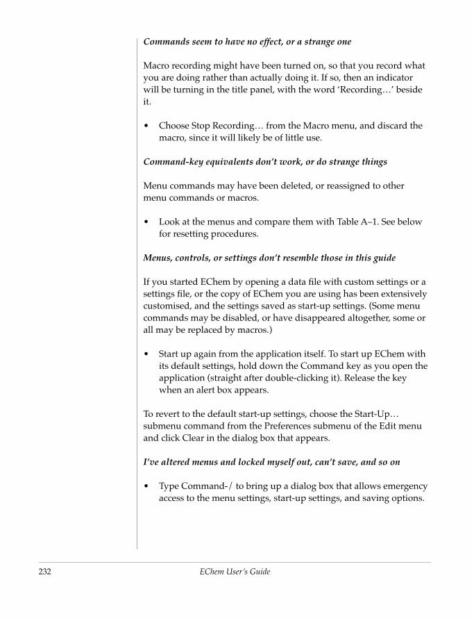
232
Commands seem to have no effect, or a strange one
Macro recording might have been turned on, so that you record what you are doing rather than actually doing it. If so, then an indicator will be turning in the title panel, with the word ‘Recording…’ beside it.
• Choose Stop Recording… from the Macro menu, and discard the macro, since it will likely be of little use.
Command-key equivalents don’t work, or do strange things
Menu commands may have been deleted, or reassigned to other menu commands or macros.
• Look at the menus and compare them with Table A–1. See below for resetting procedures.
Menus, controls, or settings don’t resemble those in this guide
If you started EChem by opening a data file with custom settings or a settings file, or the copy of EChem you are using has been extensively customised, and the settings saved as start-up settings. (Some menu commands may be disabled, or have disappeared altogether, some or all may be replaced by macros.)
• Start up again from the application itself. To start up EChem with its default settings, hold down the Command key as you open the application (straight after double-clicking it). Release the key when an alert box appears.
EChem User’s Guide
To revert to the default start-up settings, choose the Start-Up… submenu command from the Preferences submenu of the Edit menu and click Clear in the dialog box that appears.
I’ve altered menus and locked myself out, can’t save, and so on
• Type Command-/ to bring up a dialog box that allows emergency access to the menu settings, start-up settings, and saving options.
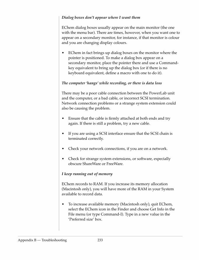
Appendix B — Troublesho
Dialog boxes don’t appear where I want them
EChem dialog boxes usually appear on the main monitor (the one with the menu bar). There are times, however, when you want one to appear on a secondary monitor, for instance, if that monitor is colour and you are changing display colours.
• EChem in fact brings up dialog boxes on the monitor where the pointer is positioned. To make a dialog box appear on a secondary monitor, place the pointer there and use a Command-key equivalent to bring up the dialog box (or if there is no keyboard equivalent, define a macro with one to do it).
The computer ‘hangs’ while recording, or there is data loss
There may be a poor cable connection between the PowerLab unit and the computer, or a bad cable, or incorrect SCSI termination. Network connection problems or a strange system extension could also be causing the problem.
• Ensure that the cable is firmly attached at both ends and try again. If there is still a problem, try a new cable.
• If you are using a SCSI interface ensure that the SCSI chain is terminated correctly.
• Check your network connections, if you are on a network.
• Check for strange system extensions, or software, especially obscure ShareWare or FreeWare.
oting 233
I keep running out of memory
EChem records to RAM. If you increase its memory allocation (Macintosh only), you will have more of the RAM in your System available to record data.
• To increase available memory (Macintosh only), quit EChem, select the EChem icon in the Finder and choose Get Info in the File menu (or type Command-I). Type in a new value in the ‘Preferred size’ box.
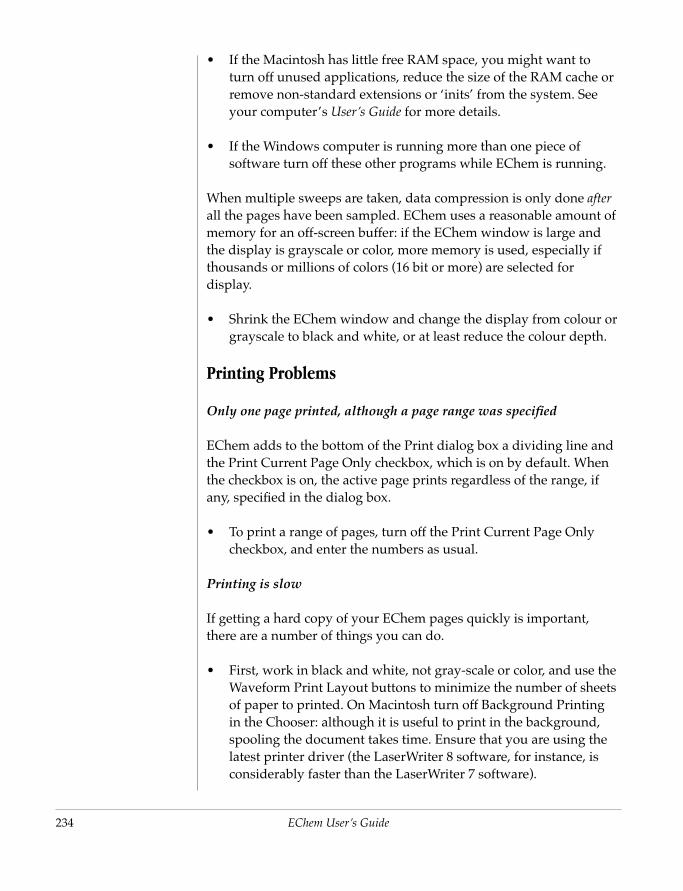
234
• If the Macintosh has little free RAM space, you might want to turn off unused applications, reduce the size of the RAM cache or remove non-standard extensions or ‘inits’ from the system. See your computer’s User’s Guide for more details.
• If the Windows computer is running more than one piece of software turn off these other programs while EChem is running.
When multiple sweeps are taken, data compression is only done after all the pages have been sampled. EChem uses a reasonable amount of memory for an off-screen buffer: if the EChem window is large and the display is grayscale or color, more memory is used, especially if thousands or millions of colors (16 bit or more) are selected for display.
• Shrink the EChem window and change the display from colour or grayscale to black and white, or at least reduce the colour depth.
Printing Problems
Only one page printed, although a page range was specified
EChem adds to the bottom of the Print dialog box a dividing line and the Print Current Page Only checkbox, which is on by default. When the checkbox is on, the active page prints regardless of the range, if any, specified in the dialog box.
• To print a range of pages, turn off the Print Current Page Only checkbox, and enter the numbers as usual.
EChem User’s Guide
Printing is slow
If getting a hard copy of your EChem pages quickly is important, there are a number of things you can do.
• First, work in black and white, not gray-scale or color, and use the Waveform Print Layout buttons to minimize the number of sheets of paper to printed. On Macintosh turn off Background Printing in the Chooser: although it is useful to print in the background, spooling the document takes time. Ensure that you are using the latest printer driver (the LaserWriter 8 software, for instance, is considerably faster than the LaserWriter 7 software).

Appendix B — Troublesho
• The Page Setup options affect printing speed. For a PostScript laser printer, Faster Printing should be on, and Color and High-Resolution Printing off. If you have another type of printer, you should experiment with the Page Setup options to see which give greatest speed. (Remember that the Faster Printing option in the EChem Page Setup dialog box is not necessarily a panacea, in fact, depending on your particular setup, it is possible that it could make printing slower.) If using the LaserWriter 8 software, leave the Layout option in the Page Setup dialog box at ‘1 Up’ (printing one page per sheet) — rescaling is quite slow.
The quality of printed work using these settings should be sufficient for most routine purposes, although, for publication quality diagrams, you may want to transfer data to a specialist graphing program such as IGOR Pro.
Printing speed depends on hardware as well: the faster the computer and printer, the faster that material can be printed.
Graphs are shrunk or comments truncated when printed
The file title, page number, and any page comments are included in the printed EChem page. Long comments mean the area used for the drawing is reduced; very long comments will be truncated.
• You cannot prevent page comments from printing, so keep them short (300 characters at most). Transfer longer comments as text to a word-processing program.
Macro Problems
oting 235
Macros behave unexpectedly
• Make sure that you have the right macro, not a different one of the same name (in the case of name conflicts, the latest macro loaded into memory is used).
• Check that you have the steps and effects recorded somewhere, and that you haven’t remembered them incorrectly–it is very easy to do.
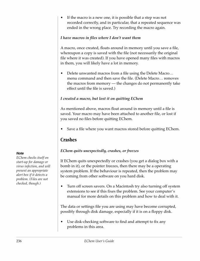
236
NoteEChem checks itself on start-up for damage or virus infection, and will present an appropriate alert box if it detects a problem. (Files are not checked, though.)
• If the macro is a new one, it is possible that a step was not recorded correctly, and in particular, that a repeated sequence was ended in the wrong place. Try recording the macro again.
I have macros in files where I don’t want them
A macro, once created, floats around in memory until you save a file, whereupon a copy is saved with the file (not necessarily the original file where it was created). If you have opened many files with macros in them, you will likely have a lot in memory.
• Delete unwanted macros from a file using the Delete Macro… menu command and then save the file. (Delete Macro… removes the macros from memory — the changes do not permanently take effect until the file is saved.)
I created a macro, but lost it on quitting EChem
As mentioned above, macros float around in memory until a file is saved. Your macro may have been attached to another file, or lost if you saved no files before quitting EChem.
• Save a file where you want macros stored before quitting EChem.
Crashes
EChem quits unexpectedly, crashes, or freezes
If EChem quits unexpectedly or crashes (you get a dialog box with a bomb in it), or the pointer freezes, then there may be a operating
EChem User’s Guide
system problem. If the behaviour is repeated, then the problem may be coming from other software on you hard disk.
• Turn off screen savers. On a Macintosh try also turning off system extensions to see if this fixes the problem. See your computer’s manual for more details on this problem and how to deal with it.
The data or settings file you are using may have become corrupted, possibly through disk damage, especially if it is on a floppy disk.
• Use disk-checking software to find and attempt to fix any problems in this area.
Appendix B — Troublesho
It may be that the EChem software itself has become damaged in some way.
• Try reinstalling EChem from the original CD.
It could be that a computer virus is causing the problems.
• Check your disk with anti-viral software. If you find a virus, you should check all potentially affected computers, disks, and backups, and eliminate the infection. See if you can find the cause of the outbreak (poor network security or student copying of software onto lab machines, for example) and try to prevent future occurrences.
Noise
The detection of small current signals can be hampered by a relatively large amount of noise. The determination of the source(s) of the noise and its elimination can be a time consuming task. The following advice is meant only as a guide to the likely sources of noise and is by no means a comprehensive list.
If you are using the ADInstruments Potentiostat, much high frequency noise can be effectively removed by setting the 10 Hz filter setting. Remember, however, that this filter will affect results from experiments that use short pulses (< 0.1 s), or fast scan times and should not be used under such conditions.
EChem voltammograms show unexpected oscillations
oting 237
The noise on the raw signal is probably large. Check by opening the Input Amplifier or Potentiostat dialog and examining the raw signal at the same gain range as your experiment.
If the ‘noise’ is 50 Hz or 60 Hz mains interference then the regular sampling periods of EChem can cause an aliasing effect which may produce low frequency oscillations in the voltammogram. In this case:
• Set the sampling period to an exact multiple of 20 ms (if using 50 Hz mains power) or 16.7 ms (if using 60 Hz mains power). The mains induced noise will be eliminated when the signal is averaged over each sampling period; or
238
• Adjust the filter setting on your potentiostat to less than 50 Hz so that the noise is reduced to an acceptable level. This will only be possible at slower scan rates as filtering will distort peak shapes at faster scan rates. A 10 Hz filter setting can be used even for quantitative linear sweep or cyclic voltammetry up to about 100 mV/s and for qualitative work up to about 500 mV/s. For pulse techniques the pulse widths should be longer than about 100 ms if a 10 Hz filter setting is employed.
• Make sure that power cables are positioned well away from your experiment and the electrodes.
Other high frequency noise
Other high frequency noise may come from fluorescent lighting, air conditioners, electric motors (in laboratories these are found in hotplate-stirrers, water bath thermostat-stirrers, and refrigerators). Occasionally equipment in adjacent rooms may be the cause of the problem.
• Turn off lights, and nearby equipment, one at a time to locate noise source(s) by trial and error
The computer itself, or other nearby computers, are likely sources of high frequency noise. The computer monitor and the floppy and hard disk drives are the most common origins.
• Reposition the potentiostat and reaction vessel as far from the computer as possible. Especially avoid having the electrodes in front of the computer monitor.
EChem User’s Guide
Occasional spikes or intermittent noise
Occasional spikes or intermittent noise are more likely to be caused by nearby electrical instrumentation being turned on or off. Remember that many instruments have internal relays that may be switching on and off during normal operation. The computer hard disk and floppy disk drives may also give rise to this type of noise.
• Install a surge suppressor/line filter power board on your power socket and plug the computer, MacLab/PowerLab and
Appendix B — Troublesho
potentiostat all into this one board. Try running your experiment with nearby equipment switched off.
Noise with no apparent cure
Aluminium foil wrapped around the electrochemical cell and grounded at a single common place may help. Placing the experiment, potentiostat, MacLab or PowerLab, and even the computer on a single large grounded copper sheet may reduce noise levels markedly. In very low current or very noisy situations you may have no alternative but to enclose your experiment in a Faraday cage. Commercial cages are available but they will work no better than one made by a local tradesperson from sheet metal or copper mesh. It may also be useful to position the potentiostat within the cage. In a large laboratory a small garden shed could be used as a walk-in cage.
oting 239

240
EChem User’s Guide
EChem
User’s GuideC
A P P E N D I X CTechnique Summary
This Appendix provides a quick reference to the techniques provided
in then EChem Technique menu. It is not a replacement for the detail
given in Chapter 7. If you need more detail please refer to the
appropriate technique in Chapter 7.
This Appendix does not cover the additional techniques described in
Chapter 8.
241

242
Parameter
Range 1000, 20full scale
Initial Potential between
Final Potential between
Scan Rate usually 5
Step Width ≥ 0.1 ms
Step Height 1-2 mV
Samplig Period ≥ 0.1 ms
Steps automat
Rest Time 1–5 s is
Table C–1 Linear Sweep Voltammetry parameter reference
Linear Sweep VoltammetryIn linear sweep voltammetry (LSV) a linearly increasing (or decreasing) potential staircase ramp is applied to the working electrode (Figure C–1). The average current flowing during the sample periods (at the end of each step) in the potential ramp is recorded and plotted against the voltage.
The current is usually sampled at the end of each potential step. If you use the Multi Pulse Technique to set up a linear sweep run then you can alter the position of the sampling period.
Values Comments
00 or 5000 mV The 2000 mV range is typical
±1, 2 or 5 V
±1, 2 or ±5 V Must not be the same as the initial potential. It can be more negative or positive than the initial potential.
–1000 mV/s Faster scan rates lead to a higher background signals unless microelectrodes are employed.
The time that the potential is kept constant at each step
is ideal Values over 10 mV give insufficient potential resolution and lead to
EChem User’s Guide
excessively high charging currents
Use 20 ms at 50 Hz power, or 16.7 ms at 60 Hz power, to minimise mains hum interference (visible as oscillations on voltammogram)
ically set
usual The length of time the potential is kept at the initial potential before the scan is started.
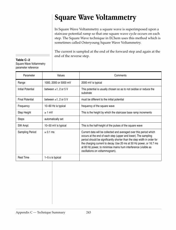
Appendix C — Technique
Parameter
Range 1000,
Initial Potential betwee
Final Potential betwee
Frequency 10–60
Step Height ≥ 1 mV
Steps autom
SW Ampl. 10–50
Sampling Period ≥ 0.1 m
Rest Time 1–5 s i
Table C–2 Square Wave Voltammetry parameter reference
Square Wave VoltammetryIn Square Wave Voltammetry a square wave is superimposed upon a staircase potential ramp so that one square wave cycle occurs on each step. The Square Wave technique in EChem uses this method which is sometimes called Osteryoung Square Wave Voltammetry.
The current is sampled at the end of the forward step and again at the end of the reverse step.
Values Comments
2000 or 5000 mV 2000 mV is typical
n ±1, 2 or 5 V This potential is usually chosen so as to not oxidise or reduce the substrate
n ±1, 2 or 5 V must be different to the initial potential
Hz is typical frequency of the square wave
This is the height by which the staircase base ramp increments
atically set
mV is typical This is the half-height of the pulses of the square wave
s Current data will be collected and averaged over this period which occurs at the end of each step (upper and lower). The sampling period should be significantly shorter than the step width in order for the charging current to decay. Use 20 ms at 50 Hz power, or 16.7 ms at 60 Hz power, to minimise mains hum interference (visible as
Summary 243
oscillations on voltammogram).
s typical

244
Parameter
Range 1000, 2
Initial Potential betwee
Final Potential betwee
Scan Rate usually
Step Width 2–4 s is
Step Height 10 mV i
Steps automa
Pulse Width 5–100 m
Rest Time several
Sampling Period ≥0.1 ms
Table C–3 Pulse Voltammetry parameter reference
Normal & Reverse Pulse VoltammetryIn Normal Pulse Voltammetry, a series of pulses of successively larger potential are applied above a base potential to the working electrode. Reverse Pulse Voltammetry is similar except that the base potential is chosen to electrolyse the electroactive substrate. The pulses that are then applied cause the reverse reaction to take place. The current is sampled at the end of each pulse, and plotted against the potential.
Values Comments
000 or 5000 mV 2000 mV is typical
n ±1, 2 V or 5 V Usually chosen to be a value at which the electrode reaction of interest does not occur. For Reverse Pulse Voltammetry this potential is chosen to cause complete oxidation (or reduction) of the substrate, and the pulses then cause the reverse reaction.
n ±1, 2 or 5 V This is the height of the last pulse to be applied. It can be thought of as the height of an imaginary ramp passing through the tops of the pulses.
5–100 mV/s Usually this parameter is allowed to vary as the Step Width and Step Height are set.
typical This is the period of a single step (including the pulse time). Much shorter times can be used with microelectrodes.
s typical This defines the increase in height (mV) of successive pulses. The minimum increment available is 1 mV
EChem User’s Guide
tically set
s is typical Should be wide enough to allow the non-faradaic components of the current to decay before sampling. Much shorter times can be used with microelectrodes.
seconds This is the period between when the deposition potential is applied and the scan commences. It allows the solution to come to equilibrium after the initial potential is applied.
The current is always sampled at the end of the pulse. Use 20 ms at 50 Hz power, or 16.7 ms at 60 Hz power, to minimise mains hum interference (visible as oscillations on voltammogram)
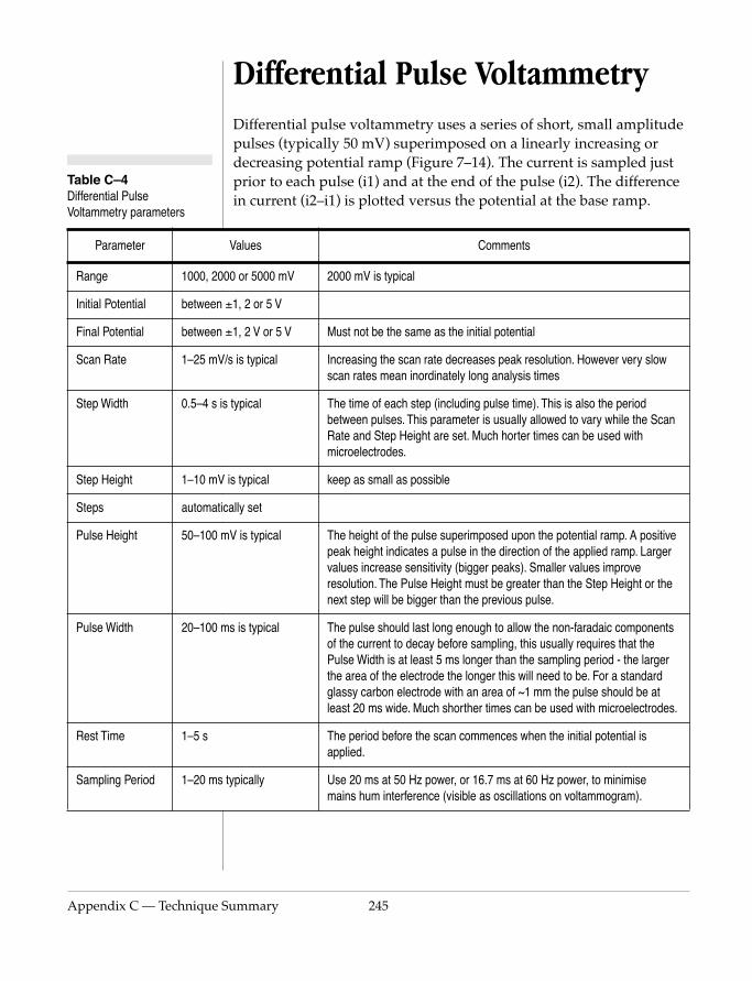
Appendix C — Technique
Parameter
Range 1000, 20
Initial Potential between
Final Potential between
Scan Rate 1–25 mV
Step Width 0.5–4 s
Step Height 1–10 mV
Steps automat
Pulse Height 50–100
Pulse Width 20–100
Rest Time 1–5 s
Sampling Period 1–20 ms
Table C–4 Differential Pulse Voltammetry parameters
Differential Pulse VoltammetryDifferential pulse voltammetry uses a series of short, small amplitude pulses (typically 50 mV) superimposed on a linearly increasing or decreasing potential ramp (Figure 7–14). The current is sampled just prior to each pulse (i1) and at the end of the pulse (i2). The difference in current (i2–i1) is plotted versus the potential at the base ramp.
Values Comments
00 or 5000 mV 2000 mV is typical
±1, 2 or 5 V
±1, 2 V or 5 V Must not be the same as the initial potential
/s is typical Increasing the scan rate decreases peak resolution. However very slow scan rates mean inordinately long analysis times
is typical The time of each step (including pulse time). This is also the period between pulses. This parameter is usually allowed to vary while the Scan Rate and Step Height are set. Much horter times can be used with microelectrodes.
is typical keep as small as possible
ically set
mV is typical The height of the pulse superimposed upon the potential ramp. A positive peak height indicates a pulse in the direction of the applied ramp. Larger values increase sensitivity (bigger peaks). Smaller values improve resolution. The Pulse Height must be greater than the Step Height or the next step will be bigger than the previous pulse.
ms is typical The pulse should last long enough to allow the non-faradaic components
Summary 245
of the current to decay before sampling, this usually requires that the Pulse Width is at least 5 ms longer than the sampling period - the larger the area of the electrode the longer this will need to be. For a standard glassy carbon electrode with an area of ~1 mm the pulse should be at least 20 ms wide. Much shorther times can be used with microelectrodes.
The period before the scan commences when the initial potential is applied.
typically Use 20 ms at 50 Hz power, or 16.7 ms at 60 Hz power, to minimise mains hum interference (visible as oscillations on voltammogram).
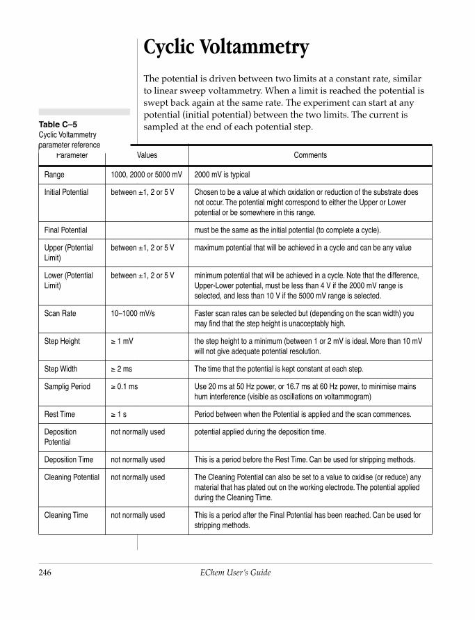
246
Parameter
Range 1000, 20
Initial Potential between
Final Potential
Upper (Potential Limit)
between
Lower (Potential Limit)
between
Scan Rate 10–1000
Step Height ≥ 1 mV
Step Width ≥ 2 ms
Samplig Period ≥ 0.1 ms
Rest Time ≥ 1 s
Deposition Potential
not norm
Deposition Time not norm
Cleaning Potential not norm
Cleaning Time not norm
Table C–5 Cyclic Voltammetry parameter reference
Cyclic VoltammetryThe potential is driven between two limits at a constant rate, similar to linear sweep voltammetry. When a limit is reached the potential is swept back again at the same rate. The experiment can start at any potential (initial potential) between the two limits. The current is sampled at the end of each potential step.
Values Comments
00 or 5000 mV 2000 mV is typical
±1, 2 or 5 V Chosen to be a value at which oxidation or reduction of the substrate does not occur. The potential might correspond to either the Upper or Lower potential or be somewhere in this range.
must be the same as the initial potential (to complete a cycle).
±1, 2 or 5 V maximum potential that will be achieved in a cycle and can be any value
±1, 2 or 5 V minimum potential that will be achieved in a cycle. Note that the difference, Upper-Lower potential, must be less than 4 V if the 2000 mV range is selected, and less than 10 V if the 5000 mV range is selected.
mV/s Faster scan rates can be selected but (depending on the scan width) you may find that the step height is unacceptably high.
the step height to a minimum (between 1 or 2 mV is ideal. More than 10 mV will not give adequate potential resolution.
The time that the potential is kept constant at each step.
Use 20 ms at 50 Hz power, or 16.7 ms at 60 Hz power, to minimise mains hum interference (visible as oscillations on voltammogram)
EChem User’s Guide
Period between when the Potential is applied and the scan commences.
ally used potential applied during the deposition time.
ally used This is a period before the Rest Time. Can be used for stripping methods.
ally used The Cleaning Potential can also be set to a value to oxidise (or reduce) any material that has plated out on the working electrode. The potential applied during the Cleaning Time.
ally used This is a period after the Final Potential has been reached. Can be used for stripping methods.
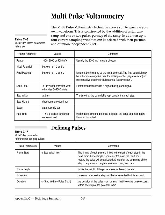
Appendix C — Technique
Ramp Parameter
Range 1000,
Initial Potential betwe
otherw
Step Width ≥ 2 m
Step Height depen
Steps autom
Rest Time 1–5 s corros
Pulse Parameters
Pulse Start < Step
Pulse Height
Increment
Duration < (Step
Table C–6 Multi Pulse Ramp parameter reference
Table C–7 Multi Pulse parameter reference for defining pulses
Multi Pulse VoltammetryThe Multi Pulse Voltammetry technique allows you to generate your own waveform. This is constructed by the addition of a staircase ramp and one or two pulses per step of the ramp. In addition up to four current sampling windows can be selected with their position and duration independently set.
Defining Pulses
Values Comment
2000 or 5000 mV Usually the 2000 mV range is chosen.
en ±1, 2 or 5 V
en ±1, 2 or 5 V Must not be the same as the initial potential. The final potential may be either more negative than the initial potential (negative scan) or more positive than the initial potential (positive scan).
V/s for corrosion work ise 5–1000 mV/s
Faster scan rates lead to a higher background signal.
s The time that the potential is kept constant at each step.
dent on experiment
atically set
is typical, longer for ion work
the length of time the potential is kept at the initial potential before the scan is started
Final Potential betwe
Scan Rate < 1 m
Summary 247
Values Comments
Width (ms) The timing of each pulse is linked to the start of each step in the base ramp. For example if you enter 20 ms in the Start box it means the pulse will be activated 20 ms after the beginning of the step. The pulse can begin at any time during each step
this is the height of the pulse above (or below) the step.
pulses on successive steps will be incremented by this amount
Width – Pulse Start) the duration of the pulse must be such that the entire pulse occurs within one step of the potential ramp

248
EChem User’s Guide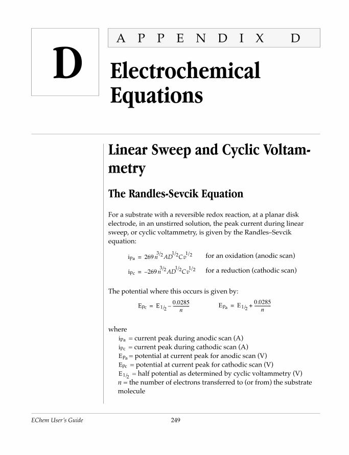
EChem
User’s GuideD
A P P E N D I X DElectrochemicalEquations
Linear Sweep and Cyclic Voltam-metry
The Randles-Sevcik Equation
For a substrate with a reversible redox reaction, at a planar disk electrode, in an unstirred solution, the peak current during linear sweep, or cyclic voltammetry, is given by the Randles–Sevcik equation:
for an oxidation (anodic scan)
for a reduction (cathodic scan)
ipa 269 n3/2AD
1/2Cv1/2=
ipc 269 n3/2AD
1/2Cv1/2–=
249
The potential where this occurs is given by:
where = current peak during anodic scan (A) = current peak during cathodic scan (A)= potential at current peak for anodic scan (V) = potential at current peak for cathodic scan (V) = half potential as determined by cyclic voltammetry (V)
n = the number of electrons transferred to (or from) the substrate molecule
Epa E1/20.0285
n----------------+=Epc E1/2
0.0285n
----------------–=
ipa
ipc
Epa
Epc
E1/2

250
A = area of the exposed surface of the electrode (cm2)D = diffusion coefficient of the substrate molecule (cm2 s-1).C = concentration of the substrate molecule (mol L-1)υ = the scan rate (V s-1)
The factor of 269 is a parameter that derives from using a planar electrode at a temperature of 298 K
Thus a truly reversible reaction can be identified by examining the adherence of the system to the following functions:
•
• Ep independence of the san rate, υ
In addition cyclic voltammograms will exhibit:
mV (at 298 K)
When working in highly resistive solutions, which is often the case when using organic solvents for cyclic voltammetry, the reference electrode should be kept as close as possible to the working electrode to minimise iR drop. Nonetheless there may still be an appreciable uncompensated resistance which will cause | Epc - Epa| to become larger than predicted, the peaks will be broader and the peak currents smaller.
ip v∝
Epa Epc– 57n------=
ipaipc------ 1=
EChem User’s Guide

Appendix D – Electrochem
Differential Pulse Techniques
The Parry-Osteryoung Equation
Differential pulse techniques require that the sampling periods be chosen so that the current is only due to a Faradaic component (i.e. only due to a redox reaction and not the charging current which dominates immediately after the application of a pulse)
The observed potential of the peak when studying a reversible system is given by:
whereEp = potential at which the peak occurs
= the half wave potential (as might determined by cyclic voltammetry)hp = the height of the pulse.
The peak current is given by the Parry-Osteryoung equation:
where
Ep E1/2h p2
------–=
E1/2
ipnFAD
1 2⁄ C 1 θ–( )
1000π1 2⁄ τ( t )–
1 2⁄ 1 θ+( )----------------------------------------------------------------=
ical Equations 251
t = time at which the current is first sampled in each cycleτ = time at which the current is sampled second in each cycle
n = the number of electrons transferred to (or from) the substrate moleculeF = Faraday's constant, 96485 C mol-1
A = area of the exposed surface of the electrode (cm2)D = diffusion coefficient of the substrate molecule (cm2 s-1).C = concentration of the substrate molecule (mol L-1)R = the gas constant, 8.314 J K-1 molT = the temperature (K)
θ enFAh p( )
2RT-----------------------
=

252
Chronoamperometry
The Cottrell Equation
When chronoamperometry is performed on an unstirred solution at a planar electrode the faradaic current response is described by the Cottrell equation
where
n = the number of electrons transferred to (or from) the substrate moleculeF = Faraday's constant, 96485 C mol-1
A = area of the exposed surface of the electrode (cm2)D = diffusion coefficient of the substrate molecule (cm2 s-1).C = concentration of the substrate molecule (mol L-1)t = time (s)
The factor of 1000 is to bring both cm and dm (1 L = 1 dm3) in the equation to common units.
In aqueous solution the coefficient of diffusion usually has a value of between 10-5 and 10-6 cm2 s-1.
inFAD
1 2⁄ C
1000π1 2⁄ t
1 2⁄--------------------------------=
EChem User’s Guide

Appendix D – Electrochem
Chronocoulometry
The Integrated Cottrell Equation
The current response equation at a planar electrode for a chronocoulometric experiment is the time integrated form of the Cottrell equation:
whereQ = the number coulombs transferredn = the number of electrons transferred to (or from) the substrate moleculeA = area of the exposed surface of the electrode (cm2)D = diffusion coefficient of the substrate molecule (cm2 s-1).C = concentration of the substrate molecule (mol L-1)t = time (s)k = a constant.
Thus a plot of Q versus t1/2 should produce a straight line with an intercept of k.
The constant k can be defined as: k = nFAΓ + Qdl
whereΓ = surface concentration of adsorbed substrate (mol cm-2)
Q i td0
t∫ 2nFAD
1 2⁄ Ct1 2⁄
1000π1 2⁄
---------------------------------------- k+= =
ical Equations 253
Qdl = double layer charging.

254
EChem User’s Guide
EChem
WARNAll orga lessertoxic, aflammaprocedin a wefume hall butsolveneye prorubberglassesis relatorganipenetrcarryinsolutesSimilaused ware toxirritanfamiliathe potreadingSafety availabof solvAlwaycomposafety availabhandle
User’s Guide
E
INGanic solvents are, to or greater degree, nd many are ble. General safety
ures include working ll ventilated area (a ood is necessary for the most benign ts), with hand and tection (usually gloves and safety ). Even if the solvent ively harmless most c solvents can ate the skin easily g potentially toxic with them. rly most electrolytes ith organic solvents ic and/or skin ts. Always rize yourself with ential hazards by the Materials
Data Sheets le from the suppliers
ents and electrolytes. s assume that new unds (for which no data may be le) are toxic and them with due care.
A P P E N D I X E
Cyclic Voltammetry,Solvents & Electrolytes
Common organic solvents for cyclic voltammetry include methanol, ethanol, propylene carbonate, 1,2-dimethoxyethane, acetonitrile, acetone, dimethylsulfoxide (dmso), dichloromethane, dichloroethane, and toluene. Polar and protic solvents exhibit lower resistivities than non-polar and/or aprotic solvents. Unfortunately it is the more resistive solvents in which common electrolytes are least soluble.
Remember that many of the constituent ions (both cations and anions) of electrolytes are toxic and that when dissolved in organic solvents they can be carried across the skin. Similar aqueous solutions are usually much less of a hazard if skin contact occurs. However, in all cases of accidental spillage where you do not know the specific treatment, all contaminated skin areas should be continuously flushed with copious amounts of water for at least several minutes.
For a a good general introduction to the use of non-aqueous solvents see the ‘Chapter 7, Solvents and Electrolytes’ in ‘Electrochemistry for
255
Chemists’, 2nd edition, D. T. Sawyer, A. Sobkowiak, and J. L. Roberts, Wiley-Interscience New York, 1995.
Solubility Rules
Some generalised rules for solubility of electrolytes in organic solvents are:
• perchlorates (care! explosion hazard), chlorides, nitrates, and tosylates are most soluble in alcohols;

256
• perchlorate in the presence of potassium ions will give a precipitate of KClO4;
• electrolytes comprising large cations and anions will be more soluble in non-polar solvents and less soluble in polar solvents;
• dimethylsulfoxide is a very good solvent for most electrolytes;
• fluoroborate and hexafluorophosphate salts exhibit particularly good solubility in acetone and acetonitrile;
• dichloromethane and similar solvents usually require tetra-n-butylammonium hexafluorophosphate.
• electrochemistry in toluene an be performed using liquid tetrabutylammonium tetrafluoroborate toluene solvate. See J. Chem. Soc. Chem. Commun, 323 (1985).
Solvent Stability
Amides, esters, nitriles, strained ethers, etc. are subject to hydrolysis especially if traces of acid or base are present. Hydrolysis reactions can be very slow (hours or days) and often manifest themselves as an increase in background currents or a reduced redox stability window. Remember that only a small fraction of the solvent need hydrolyze to generate impurities that can be detected electrochemically but which will remain unseen by nmr or infrared spectroscopy.
Use of Large Ions as Electrolytes
EChem User’s Guide
A wide variety of large cations and anions are available so that in practice it is nearly always possible to find an electrolyte that will be suitable for a given solvent. Common electrolytes are commercially available but others will need to be prepared by the user. Purity of both commercial and home made electrolytes should be checked by performing a blank run at the same sensitivity setting of the potentiostat that is used when the analyte is present. Remember that purity is a relative term – electrolyte and solvent that has been used satisfactorily with high concentrations of analyte at low sensitivity settings may prove to hopelessly contaminated when used with much lower concentrations of analyte at very high sensitivity settings.
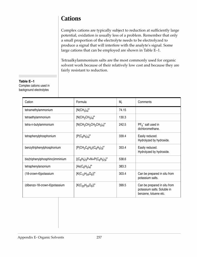
Appendix E- Organic Solv
Cation
tetramethylammonium
tetraethylammonium
tetra-n-butylammonium
tetraphenylphosphonium
benzyltriphenylphosphoniu
bis(triphenylphosphino)imm
tetraphenylarsonium
(18-crown-6)potassium
(dibenzo-18-crown-6)potas
Table E–1 Complex cations used in background electrolytes
Cations
Complex cations are typically subject to reduction at sufficiently large potential, oxidation is usually less of a problem. Remember that only a small proportion of the electrolyte needs to be electrolyzed to produce a signal that will interfere with the analyte's signal. Some large cations that can be employed are shown in Table E–1.
Tetraalkylammonium salts are the most commonly used for organic solvent work because of their relatively low cost and because they are fairly resistant to reduction.
Formula Mr Comments
[N(CH3)4]+ 74.15
[N(CH2CH3)4]+ 130.3
[N(CH2CH2CH2CH3)4]+ 242.5 PF6– salt used in
dichloromethane.
[P(C6H5)4]+ 339.4 Easily reduced.Hydrolyzed by hydroxide.
m [P(CH2C6H5)(C6H5)3]+ 353.4 Easily reduced.Hydrolyzed by hydroxide.
inium [(C6H5)3P=N=P(C6H5)3]+ 538.6
ents 257
[As(C6H5)4]+ 383.3
[K(C12H24O6)]+ 303.4 Can be prepared in situ from potassium salts.
sium [K(C20H24O6)]+ 399.5 Can be prepared in situ from potassium salts. Soluble in benzene, toluene etc.

258
Anion
nitrate
perchlorate
triflate
methanesulfonate
tosylate
trifluoroacetate
tetrafluoroborate
tetraphenylborate
hexafluorophosphate
Table E–2 Complex anions used in background electrolytes
explosion hazard and their use should be avoided wherever possible. Especially avoid evaporation of perchlorate containing solutions and clean up all spills immediately.
Anions
Large anions may be subject to reduction or oxidation. Some anions that can be employed as shown in Table E–2. Perchlorate salts are a known explosion hazard and should be avoided wherever possible. Note that while nitrate is often considered safe to use, it is an oxidizing agent. Its use as an electrolyte (at relatively high concentrations) in organic solvents is a potential explosion/fire hazard, especially if traces of acid are present, or if the solution is left to evaporate.
Formula Mr Comments
NO3– 62.00 Potential explosion hazard.
ClO4– 99.45 Explosion hazard, easily reduced.
CF3SO3– 149.1
CH3SO3– 95.09
CH3C6H4SO3– 171.2
CF3COO– 113.0
BF4– 86.80 May hydrolyze to HF.
B(C6H5)4– 319.2
PF6– 145.0 May hydrolyze to HF.
WARNINGPerchlorates are a known
EChem User’s Guide

Appendix E- Organic Solv
Electrode and Cell Design for Organic SolventsCyclic voltammetry can be carried out in ordinary sample tubes (2.5 × 5 cm) with the electrodes placed through holes in the plastic cap. Air can be excluded with an argon or nitrogen purge. Argon is more expensive but because of its greater density tends to blanket the sample more efficiently.
The purity of the solvent and the electrolyte can be established by looking for spurious signals in the cyclic voltammogram — but make sure that you run at the same gain range you will be using for your samples. In many cases both the solvent and electrolyte will need to be thoroughly dried as traces of water may limit the scan range or react with the substrate or electrolysis products.
Electrochemistry in dichloromethane or 1,2-dichloroethane (less volatile) can be performed using a 0.10 mol L-1 solution of tetra-n-butylammonium hexafluorophosphate. Other common combinations are 0.1 mol L-1 tetra-n-butylammonium tetrafluoroborate in acetonitrile, or benzonitrile; or 0.1 mol L-1 tetraethylammonium perchlorate in propylenecarbonate, tetrahydrofuran, or dimethyl formamide. Where possible perchlorates (explosion hazard) should be substituted with salts containing non-oxidizing anions.
While many workers go to great length to dry their solvents this is really only necessary if the compound or its redox products are water sensitive or if you wish to explore outside the redox inactive region of
ents 259
water. There is nothing inherently wrong in using mixed aqueous/organic solvent mixtures if this is convenient. However, remember that many molecules, or their redox products, are acids or bases and, that if your aqueous solutions are not adequately buffered, you may have difficulty in getting reproducible results. The addition of a small amount of acid or base to an aqueous solvent mixture can both serve to buffer the solution and to act as a background electrolyte.
Many studies require only a simple determination of E1/2 values for compound characterisation. In these cases some liberties can be taken with electrode design. A 0.5 mm diameter platinum wire can be used
260
as the working electrode. The wire should be embedded in a soft (soda) glass rod which can be polished at its end. Soda glass matches the thermal coefficient of platinum more closely than borosilicate — if the platinum wire and glass rod separate in the working electrode solution may seep into the electrode and give old signals. Allowing the wire to protrude by as much as 1–3 mm will increase the current but this is usually not necessary.
The auxiliary (counter) electrode is usually a simple platinum wire.
The reference Ag/AgCl electrode can be as simple as a silver wire previously anodized in 1 M hydrochloric acid, rinsed with water, then allowed to dry. The wire is then immersed in electrolyte solution in a thin glass or Teflon tube with a sintered frit at the bottom which acts as a small salt bridge.
If there is any doubt about the stability of the reference then the ferrocene/ferrocinium (Fc/Fc+) couple can be used as reference potential to calibrate the reference electrode: a small amount of ferrocene is added to the reaction mixture after the experiment is finished (the peak to peak separation is usually about 70 mV). Alternatively the electrode can be calibrated at the beginning of each day by measuring the Fc/Fc+ couple in fresh electrolyte. Cleaning and re-anodizing of the silver wire will be necessary from time to time. It is not uncommon for inorganic and organic chemists to report redox potentials relative to ferrocene.
The reference electrode should be placed as close as possible to the working electrode. Distances between the working and auxiliary electrodes should also be kept to a minimum to keep the required
EChem User’s Guide
compliance voltage small (see Appendix F).

Appendix E- Organic Solv
WARNING Concentrating perchloric acid solutions can result in serious explosion especially if organic matter is present! Under no circumstances should concentrated perchloric acid (> 1.0 M) be used in these preparations. No product (final or intermediate) should be taken to dryness unless a representative sample dissolved in a small quantity of water shows that no acid is present (use a narrow range indicator paper). All filtrates and washings should be immediately discarded by flushing down the sink with tap water.
Synthesis of Selected Electrolytes
Tetraethylammonium perchlorate, [(CH3CH2)4N]ClO4, Mr = 229.7
Acid-Bromide method
Tetraethylammonium bromide, Mr = 210.2, (100 g, 0.48 mol) is dissolved in water (100 mL) with slight warming, then 1.0 M perchloric acid (600 mL, 0.60 mol) is added. White crystals form immediately and are filtered off after cooling the mixture to below 5 °C. The crude product is washed with ice cold 1.0 M perchloric acid (100 mL) then recrystallised from 1.0 M perchloric acid (300 mL). The product is filtered off, washed first with ice cold 1.0 M perchloric acid (100 mL), then ice cold ethanol (200 mL). Recrystallisation from boiling ethanol (300 mL) with sufficient water to ensure complete dissolution (about 30 mL) gives the final product which is washed with ice cold ethanol (200 mL). The product can be checked for purity by dissolving about 0.5 g in warm water (2 mL) and testing the pH of the solution, and for any reaction with silver nitrate. A further recrystallisation from ethanol may be necessary. The product is dried under vacuum (0.1 mm Hg), to yield 70.3 g (64%) of white needles. The solid compound should be treated as an oxidising agent and stored away from reducing (organic) materials.
Acid-Base method
ents 261
Aqueous 1 M perchloric acid (250 mL, 0.25 mol) is added to a solution of 1 M tetraethylammonium hydroxide (250 mL, 0.25 mol). The mixture is adjusted to pH 7 (use a narrow range pH indicator paper, not litmus paper) by the addition of more acid or base solution as required, and stirred while cooling in an ice bath.The resulting precipitate is removed from the cold suspension by suction filtration and washed with cold water. The crude product can be recystallised from water and dried at 100°C for 24 h in vacuo. M.p. 351–352.5°C with decomposition. The solid compound should be treated as an oxidising agent and stored away from reducing (organic) materials.
The purity of the product should be checked by cyclic voltammetry.

262
WARNING Hexafluorophosphoric acid is extremely corrosive, it may also contain traces of hydrofluoric acid! Handle with gloves in a fume cupboard.Hexafluorophosphate salts can very slowly hydrolyze releasing hydrogen fluoride, thus they should be stored dry, in plastic containers.
Tetra-n-butylammonium hexafluorophos-phate, [n-Bu4N]PF6
Bromide method
A solution of tetra-n-butylammonium bromide (100 g, 0.31 mol) in acetone (250 mL) is mixed with a solution of ammonium hexafluorophosphate (50 g, 0.4 mol) in acetone (350 mL). The resulting precipitate of ammonium bromide is removed by suction filtration. The filtrate is concentrated, with a rotary evaporator, to approximately 200 mL. Water is added to the acetone solution to precipitate tetra-n-butylammonium hexafluorophosphate (final volume approximately 2 L). The precipitate is removed by suction filtration, washed with water, and then redissolved in a solution of ammonium hexafluorophosphate (5 g, 0.04 mol) in acetone (200 mL) — more acetone can be added to complete dissolution if required. Addition of water (final volume approximately 2 L) causes the precipitation of the crude product which is removed by suction filtration and washed with water.
Acid-base method
An aqueous solution of 0.5 M hexafluorophosphoric acid (600 mL, 0.3 mol) is added to an aqueous 0.5 M solution of tetra-n-butylammonium hydroxide (600 mL, 0.3 mol). The mixture is adjusted to pH 7 (use a narrow range pH indicator paper, not litmus paper) by the addition of more acid or base solution as required. The crude product is removed from the cooled mixture by suction
EChem User’s Guide
filtration and washed with water.
Recrystallisation
The crude product, produced by either the bromide or acid-base method, is recrystallized three or four times from a 3:1 mixture of ethanol/water and then dried for at least 24 h at 100°C in a vacuum oven. The yield is usually about 95 g.
The purity of the product should be checked by cyclic voltammetry.
Appendix E- Organic Solv
WARNINGTriflic acid is volatile and extremely corrosive! Handle with gloves in a fume cupboard. Tetra-n-butylammonium triflate is hygroscopic.
WARNING Fluoroboric acid is extremely corrosive, it may also contain traces of hydrofluoric acid! Handle with gloves in a fume cupboard.Fluoroboric salts can very slowly hydrolyze releasing hydrogen fluoride, thus they should be stored dry, in plastic containers.
Tetra-n-butylammonium tetrafluoroborate, [n-Bu4N]BF4, Mr = 391.5
Acid-Bromide method
Aqueous fluoroboric acid (48%, 36 mL) is added to a solution of tetra-n-butylammonium bromide (84 g, 0.25 mol) in water (180 mL) and the mixture stirred for 1 minute. The resulting precipitate is removed by suction filtration and washed with water until the washings are no longer acid (use a narrow range pH paper). The crude product can be recystallised from ethyl acetate/cyclohexane. M.p. 162–162.5°C.
The purity of the product should be checked by cyclic voltammetry.
Tetra-n-butylammonium fluoroboratetoluene solvate, [n-Bu4N]BF4.3(C6H5CH3)
Tetrabutylammonium fluoroborate is stirred in toluene between 22–25°C. A two phase mixture results. The lower layer has an approximate formula of [n-Bu4N]BF4.3(C6H5CH3). (Below 22°C the solvent-free fluoroborate salt crystallises.) This layer an be separated and used, without further purification, as the solvent for electrohemical work. Reference: J. Chem. Soc. Chem. Commun, 323 1985.
Tetra-n-butylammonium triflate[n-Bu4N]CF3SO3, Mr = 391.5
ents 263
Triflic acid (trifluoromethanesulfonic acid), Mr = 150.1, (600 mL, 0.15 mol) is slowly added, with stirring, and cooling, to a commercially available 40% solution of tetrabutylammonium hydroxide (Mr = 259.5) (100 mL 0.15 mol) until the pH drops to 6.5 (use a narrow range indicator paper). Water is added if necessary to allow adequate stirring. The crude product is suspended in ice cold water and filtered 5 times to wash it, then dried and recrystallised from a mixture of dichloromethane and diethyl ether. Reference: J. Org. Chem., 37, 3968, 1972.
The purity of the product should be checked by cyclic voltammetry.
264
CAUTION Purification and distillation of solvents should only be undertaken by an experienced chemist or laboratory technician. Incorrect procedures could lead to explosion or fire.
Appropriate care should be exercised in the handling and disposal of reactive drying agents such as metal hydrides, phosphorous pentoxide (P2O5), and sodium wire.
Adequate ventilation must be ensured about the distillation apparatus to prevent the buildup of flammable and toxic solvent vapours.
Purification of solventsFor guidelines on the purification of many solvents see “Purification of Laboratory Chemicals”, 4th edition, W. L. F. Armarego and D. D. Perrin, Butterworth-Heinemann, 1997, ISBN 0750637617.
Solvents should be of at least AR (analytical reagent) grade otherwise they may be grossly wet or otherwise need a preliminary purification step. Further drying and purification is then usually necessary before the solvent can be used for cyclic voltammetry or other electroanalytical techniques.
Distillation of solvents should always take place using a short fractionating column filled with glass rings to prevent an aerosol of the boiling solvent being carried through the condensor. A dedicated still for each solvent is ideal.
Ethers (including tetrahydrofuran, diethyl ether, 1,4-dioxan, and 1,2-dimethoxyethane), as well as aromatic hydrocarbons (benzene, toluene, xylenes) can be first dried over sodium wire then distilled from freshly drawn sodium wire with a little benzophenone added to the distillation pot. A dark blue or purple color should develop and persist during reflux, for at least 10 minutes, which signals the presence of sodium benzophenone ketyl (a radical anion). The ketyl can only exist in the absence of water. The anhydrous solvent can then be distilled. Excess sodium wire is destroyed by allowing the distillation pot to cool and cautiously adding absolute ethanol.
Dichloromethane, 1,2-dichloroethane, cyclohexane, or hexane, can be
EChem User’s Guide
dried by distillation from either P2O5 or from CaH2.
Acetonitrile should be predried using a molecular sieve with a pore size of not greater than 4 Å. Distillation can take place after reflux with a small quantity of P2O5 (about 0.5% w/v) to remove the residual water. Avoid using too much P2O5 to prevent excessive formation of an orange polymeric material.
Dimethyl sulfoxide or dimethylformamide should be predried using a molecular sieve with a pore size of not greater than 4 Å, followed by distillation at reduced pressure (10 – 20 mmHg).

Appendix E- Organic Solv
WARNINGElemental mercury and its salts and their solutions are highly toxic. Only an experienced chemist or laboratory technician. aware of the correct handling and disposal procedures should undertake work with mercury.
Supercritical FluidsThe use of supercritical fluids as solvents for cyclic voltammetry has also been investigated. For an example of a recent paper see “Electrochemical investigations in liquid and supercritical 1,1,1,2-tetrafluoroethane (HFC 134a) and difluoromethane (HFC 32)”, Andrew P. Abbott, Christopher A. Eardley, John C. Harper, and Eric G. Hope, Journal of Electroanalytical Chemistry, 457, 1–4, 1998. In particular HFC 134a, with tetra-n-butyl ammonium tetrafluoroborate as electrolyte, was shown to be have an extraordinarily wide redox stability window of 9 volts.
The Mercury ElectrodeAt times it may be of use to perform cyclic voltammetry experiments in organic solvents using a mercury working electrode. Mercury dropping electrodes (MDE’s) can be used but commercial models are expensive, cumbersome to set up, require periodic cleaning and maintenance, and require the use of relatively large amounts of elemental mercury. However they do have the advantage of being able to provide a clean mercury electrode by dislodgment of the old mercury drop and allowing a new drop to form, all at the press of a button, in any solvent you require.
Mercury film electrodes (MFE’s) use much less mercury (often much less than 1%) than a MDE, and are relatively low cost. The mercury is
ents 265
usually electrodeposited as a thin film on a glassy carbon, or carbon–fiber, support electrode. However the mercury coating must be removed and replated if it is fouled or oxidised. Some workers prepare the MFE by electrodeposition from aqueous mercuric ion solutions and then wash the electrode to replace the solvent. However it is also possible to electrodeposit mercury directly in suitable organic solvents: G. Alarnes-Varela, A.L. Suárez-Fernández, A. Costa-García, Electrochimica Acta, 44, 763–772, 1998.

266
EChem User’s Guide
EChem
User’s GuideF
A P P E N D I X FPotentiostat Designs
Potentiostats are designed to maintain a known potential difference across a pair of electrodes while measuring the resulting current flow. While this sounds simple in theory, the practice of electrochemistry has demanded a variety of designs to cope with different types of experiment.
Two electrode systemsThe simplest potentiostat is a two-electrode unit that connects to a working and reference electrode. A battery connected to two electrodes with an ammeter in series could be considered as a very simple example.
However, to maintain a known potential at the working electrode the reference electrode must exhibit a steady response. This is not easy as the current passing through the electrode will electrolyze (reduce or
267
oxidize) either the electrode material itself or material around the electrode, which in turn will alter the half cell potential. In days gone by the effects of this were usually minimized by making a very large reference electrode which would not be significantly disturbed by the currents flowing through it.
Today two electrode potentiostats masquerade under a variety of different names, such as:
• dissolved oxygen meters which measure the current that passes between a gold or platinum working electrode (at which a preset reducing potential is maintained, usually about –0.8 V, which is

268
called the ‘polarizing voltage’) with respect to a silver counter electrode. This is the classic Clarke type cell;
• nitric oxide meters, which are very similar to oxygen meters, but which reduce NO.
• amperometric ‘biosensor’ meters, which are very similar to the previous two types of meter but which can usually have their polarizing voltages adjusted to suit the system being measured.
• voltage clamps, which are used by neurophysiologists to study inter- and intracellular processes. These are usually exceptionally high gain instruments employing head stage amplification, capacitive compensation, and exhibiting very fast response times.
The common feature amongst all these devices is that they are used for experiments in which the current flowing through the (relatively large) reference electrode is usually measured in nanoamperes or less. These tiny currents are not sufficient to cause enough electrolysis to seriously disrupt the environment around the reference electrode.
Some of these potentiostats will also have an external input so that they can except an external voltage signal to alter the electrode potential.
Three electrode systemsMost voltammetric experiments for analytical chemistry involve currents of microamperes or greater and make use of a three electrode
EChem User’s Guide
instrument. The ADinstruments Potentiostat is of this type.
The electrodes are identified as the:
• working electrode, where the redox reaction of interest takes place;
• reference electrode, at which a constant potential is provided by a known half reaction. Virtually no current flows through this electrode because it is connected to the working electrode across a very large resistance (typically greater than 1012 Ω). This ensures

Appendix F – Types of Pot
High compliance potentiostats are an electrical shock hazard unless used strictly in accordance with the correct procedure. Read the manufacturer’s manual!
that concentrations around (and the potential of) the reference electrode is constant throughout the experiment; and an
• auxiliary (or counter) electrode, where a counter reaction takes place to maintain the electroneutrality of the solution. Thus if reduction occurs at the working electrode then oxidation must occur at the auxiliary electrode.
Compliance voltage
For most experiments involving such a potentiostat, at any given instant the potential between the working and reference electrodes is being held at a predetermined value while current flow is measured across the working and auxiliary electrodes. These are the current and potential values that are actually plotted.
But to do this some other potential must be maintained between the auxiliary and working electrodes. This potential is called the compliance voltage and, depending on the internal resistance of the cell (which in turn depends on type of solvent, total electrolyte concentration, distance between the electrodes, porosity and size of frits used to separate cell compartments, etc.) may be much greater than the observed potential of the working electrode. During an experiment it may happen that the potentiostat is unable to provide a sufficiently large voltage across the auxiliary and working electrodes to achieve the desired potential across the reference and working electrodes. In this situation the potentiostat is said to be out of compliance (or overloaded) and the results from such an experiment will be meaningless in the non-compliance region. The ADInstruments Potentiostat has a non-compliance light on its front
entiostat 269
panel which will illuminate if this occurs.
The greater the compliance voltage of a potentiostat the greater the number of cell designs with which it will be able to cope. Also, because this voltage can actually occur across the working and auxiliary electrodes, the greater the hazard from electric shock if the instrument is not used in accordance with the correct safety procedure. Most standard electronic componentry can handle ±10 V as a matter of course, and most potentiostats will exhibit a compliance voltage within this range. Greater compliance voltages will require the use of more specialist componentry, and such instruments will necessarily command a higher price.
270
It may also occur that the current flowing between the auxiliary and working electrodes is greater than the potentiostat is capable of delivering and/or measuring. This is a current overload condition. Currents can be decreased by using electrodes with a smaller surface area, using lower concentrations of analyte, or (for stripping methods) using a shorter deposition period. If EChem is being used with an ADinstruments Potentiostat and the current capability of the potentiostat (100 mA) is exceeded then an overload message appears in the Cursor Panel.
By connecting the reference and auxiliary electrode leads together most three electrode potentiostats can also be used as a two electrode system. Check with the potentiostat manufacturer if you are unsure whether your instrument can be used the way. The ADinstruments Potentiostat can be used in this way
Many manufacturers make three electrode potentiostats such as EG&G PAR, BAS, Radiometer, Solartron, AMEL, Metrohm, HEKA, Cypress, Sycopel, and ADInstruments.
Four electrode systemsThe most common four electrode potentiostat is the bipotentiostat. This is designed to work with two working electrodes and a common reference and auxiliary electrode, and can be considered a simple variant of the three electrode design. Advanced bipotentiostats can sweep the potential at each working electrode independently of one another while simpler units only allow the working electrode potentials to be adjusted independently and then held steady.
EChem User’s Guide
The bipotentiostat is used with a rotating ring disk electrode where the potentials of the ring and disk electrodes need to independently controlled. The most widely known manufacturer of these devices is PINE Instruments.
Another type of four electrode design makes use of two reference and two counter electrodes. These instruments can be employed to control the potential across a membrane or interface and to measure the resulting current flow. This type of potentiostat is not readily commercially available but a good design has been published: T. J. VanderNoot and D. J. Schiffrin, ‘Design and Evaluation of a Four-

Appendix F – Types of Pot
Electrode Potentiostat/ Voltage Clamp Suitable for AC Impedance Measurements at the Interface of Immiscible Electrolytes’, Journal of Electroanalytical Chemistry, 278, 137 – 150 (1990), and M. C. Wiles, D. J. Schiffrin, and T. J. VanderNoot, ‘Experimental Artifacts Associated with Impedance Measurements at Liquid–Liquid Interfaces’, Journal of Electroanalytical Chemistry, 278, 151 – 159 (1990).
entiostat 271

272
EChem User’s Guide
EChem
User’s GuideBibliography
Electrochemistry is a large field and there are many specialised and
general texts available, as well as journals and on line information.
The following list is meant as only as a general introduction to the
literature.
The InternetMuch useful information can be obtained from various internet web
sites such as:
http://www.electrochem.org/ — The Electrochemistry Society, Inc.
http://seac.tufts.edu/ — The Society for Electroanalytical Chemistry
273
http://electrochem.cwru.edu/estir/ — Electrochemical Science and Technology Information Resource. Lists of text books, journals,hand books, graduate schools, societies, meetings, etc
http://www.soton.ac.uk/~slt1/EchemGate.html — The Electrochemistry Gateway
http://www.yahoo.com/Science/Chemistry/Electrochemistry/ — Yahoo search engine
http://www.anachem.umu.se/jumpstation.htm — The Analytical Chemistry Springboard
http://chemweb.com/ecos/ — Electrochemistry Online Services (ECOS) from Elsevier. Includes liks to Elsevier’s electrochemistry journals.
http://www.nace.org/ — NACE Internaional ( National Association of Corrosion Engineers)

274
Text BooksFor an extensive listing of text books, from 1950 to present, consult the Electrochemical Science and Technology Information Resource (ESTIR) web site at http://electrochem.cwru.edu/estir/books.htm. Many other monographs and proceedings are available from the Electrochemical Society.
‘Surface chemistry and electrochemistry of membranes.’ T. S. Sorensen (Ed). Dekker, NY 1999.
‘Pocket handbook of electroanalytical instrumental techniques for analytical chemistry.’ J. Osteryoung, Prentice Hall, Englewood Cliffs, NJ 1998.
‘Biosensors: An Introduction.’ Brian R. Eggins. Wiley, 1998.
‘Environmental electrochemistry: fundamentals and applications in pollution abatement’. K. Rajeshwar and J.G. Ibanez. Academic, NY 1997.
‘Green functions in electrochemistry’. S. Romanowski and L. Wojtczak (Ed). Kluwer, Dordrecht, Netherlands 1997.
‘Modern Techniques in Electroanalysis.’ P. Vanysek (Ed), Wiley, NY 1996.
‘Laboratory techniques in electroanalytical chemistry (2nd edition).’ P.T. Kissinger and W.R. Heineman (Ed), Dekker, NY 1996.
EChem User’s Guide
‘Experimental Techniques in Bioelectrochemistry.’ V. Brabec, D. Walz and G. Milazzo (Ed.), Birkhauser, Basel 1996.
‘Reference electrodes, theory and practice’. Reprint of the original 1961 edition - see below. D.J.G. Ives and G.J. Janz (Ed), NACE International, Houston, TX 1996.
‘Electrochemistry for Chemists (2nd edition).’ D.T. Sawyer, A. Sobkowiak, and J.L. Roberts, Wiley, New York, 1995.

Bibliography
‘Voltammetric Methods in Brain Systems.’ A.A. Boulton, G.B. Baker, and R.N. Adams (Eds), Humana, Totowa, NJ 1995.
‘Single-Channel Recording (2nd Edition).’ Bert Sakmann and Erwin Neher (Eds), Plenum Press, New York 1995. An excellent overview of patch clamping and related techniques.
‘Analytical Electrochemistry.’ Joseph Wang. VCH Publishers, New York, 1994.
‘Electrochemistry in Organic Synthesis.’ J. Volke and F. Liska, Springer, New York, 1994.
‘Fundamentals of Electrochemical Analysis (2nd edition).’ Z. Galus, Wiley, New York, 1994.
‘Electrochemistry. Principles, Methods, and Applications.’ Christopher M. A. Brett and Anna Maria Oliveira Brett. Oxford University Press, 1993.
‘Introduction to Electrochemistry.’ D. Brynn Hibbert. Macmillian, London, 1993.
‘Industrial Electrochemistry.’ Derek Pletcher and Frank C. Walsh. Chapman and Hall, London, 1993.
‘Electrochemical Engineering.’ Frank C. Walsh. The Electrochemical Consultancy Ltd, 16 Queens Close, Romsey, SO51 8EG, England, 1993. (FAX: +44 703 676 960).
275
‘Electrode Processes.’ Derek Pletcher. The Electrochemical Consultancy Ltd, 16 Queens Close, Romsey, SO51 8EG, England, 1993. (FAX: +44 703 676 960).
‘The Materials Science of Microelectrodes.’ K. J. Backmann. Springer-Verlag, 1993.
‘Monitoring Neuronal Activity’, J. A. Stamford. IRL Press (at Oxford University Press), 1992. Includes descriptions of the construction of microelectrodes, and coated microelectrodes.

276
‘Potentiometric Water Analysis (2nd edition).’ Derek Midgley and Kenneth Torrance. Wiley, Chichester, 1991. Includes very comprehensive descriptions of the uses of ion selective electrodes.
‘Biosensors’, A. E. G. Cass. IRL Press (at Oxford University Press), 1990.
‘Microelectrodes: A Special Issue of Electroanalysis’, Electroanalysis, 2, 175–262, 1990.
‘Immobilized cells and enzymes’, J. Woodward. IRL Press (at Oxford University Press).
‘Electroanalytical Techniques in Clinical Chemistry and Laboratory Medicine.’ Joseph Wang, VCH, New York, 1988.
Handbook of Inorganic Electrochemistry. Louis Meites and Petr Zuman. CRC Press, Boca Raton, 1988. http://www.crcpress.com/
‘Polarography and Other Voltammetric Methods.’ Tom Riley and Arthur Watson. J. Wiley and Sons, Chichester, 1987.
‘Stripping Analysis.’ Joseph Wang, VCH, New York, 1985.
‘Electroanalytical Chemistry.’ J. J. Lingane. Wiley, New York, 1985.
‘Voltage and Patch Clamping with Microelectrodes’, Thomas G. Smith Jr., Harold Lecar, Stevaen J. Redman, and Peter W. Gage. American Physiological Society, 1985. Describes many useful circuits for use with microelectrodes.
EChem User’s Guide
‘Potentiometry and Potentiometric Titrations.’ E. P. Serjeant. Wiley, New York, 1984.
‘Electroanalytical Chemistry.’ Basil H. Vassos and Galen W. Ewing. Wiley, New York, 1983.
‘Modern Polarographic Methods in Analytical Chemistry.’ Alan Bond. Dekker, 1980.
‘Electrochemical Methods. Fundamentals and Applications.’ Allen J. Bard and Larry R. Faulkener. J. Wiley and Sons, New York, 1980.

Bibliography
‘Interfacial Electrochemistry.’ E. Gileadi, E. Kirowa-Eisner, and J. Penciner. VCH, Weinheim, 1981.
‘Comprehensive Treatise on Electrochemistry’. 10 volumes. Plenum Press, New York, 1980–1985.
‘Experimental Approach to Electrochemistry.’ Nicholas J. Selley. Edward Arnold, London, 1977.
‘Transient Techniques in Electrochemistry.’ D. D. Macdonald. Plenum, New York, 1977.
‘Fundamentals of Electrochemical Analysis.’ Z. Galus. Ellis Horwood, Chichester, 1976.
‘Stripping Voltammetry in Chemical Analysis.’ K. Z. Brainina. Wiley, London, 1974.
‘Priciples and Applications of Electrochemistry.’ D. R. Crow. Chapman and Hall, London, 1974.
‘Organic Electrochemistry.’ R. M. Baizer. Dekker, New York, 1973.
‘Determination of pH: Theory and Practice (2nd edition).’ R.G. Bates, Wiley, New York, 1973.
‘Synthetic Organic Electrochemistry.’ Albert J. Fry. Harper and Row, New York, 1972.
‘Electrochemical Reactions in Non-Aqueous Systems.’ Charles K.
277
Mann and Karen K. Barnes. Marcel Dekker, New York, 1970.
‘Topics in Organic Polarography.’ P. Zuman. Plenum, London, 1970.
‘Organic Polarography.’ P. Zuman and C. I. Perrin. Interscience, New York, 1969.
‘Electrochemistry at Solid Electrodes.’ R. N. Adams. Dekker, New York, 1969.
‘Electrochemical Techniques for Inorganic Chemists’. J. B. Headridge. Academic Press, London, 1969.

278
‘Coulometry in Analytical Chemistry.’ G. W. C. Milner and G. Phillips. Pergamon Press, Oxford, 1967.
‘Substituent Effects in Organic Polarography.’ P. Zuman. Plenum, London, 1967.
’Principles of Polarography.’ J. Heyrovsky and J. Kuta. Academic Press, New York, 1966.
‘Amperometric Titrations.’ John T. Stock. Interscience, New York, 1965.
‘Polarographic Techniques.’ L. Meites. Interscience, New York, 1965.
‘Alternating Current Polarography and Tensammetry.’ B. Breyer and H. H. Bauer. Interscience, New York, 1963.
‘Electroanalytical Principles.’ R. W. Murray and C. N. Reilley. Interscience, New York, 1963.
‘Controlled Potential Analysis.’ Garry A. Rechnitz. Pergamon, Oxford, 1962.
‘Electrochemical Reactions.’ G. Charlat, J. Badoz-Lambling, and B. Trémillon. Elsevier, Amsterdam, 1962.
‘Ionization Constants of Acids and Bases’. Adrien Albert and E. P. Serjeant. Methuen and Co., London, 1962.
‘The Principles of Electrochemistry.’ Duncan A. McInnes. Dover, New
EChem User’s Guide
York, 1961.
‘Reference Electrodes.’ D. J. G. Ives and G. J. Janz. Academic Press, New York, 1961. Reprinted in 1996 — see above.
‘Electrolyte Solutions.’ R. A. Robinson, and R. H. Stokes. Butterworths, London, 1959.
‘Electrolytic Preparations.’ Karl Elbs. Edward Arnold, London,1903.
‘Electrolytic Methods of Analysis.’ Berhard Neumann. Wittaker and Co., London, 1898.

Bibliography
JournalsBioelectrochemistry and Bioenergetics. Elsevier. http://chemweb.com/ecos
Biosensors and Bioelectronics, Elsevier. http://chemweb.com/ecos
Electroanalysis, Wiley–VCH.http://www.wiley-vch.de/vch/journals/2049/index.html
Electrochimica Acta. Elsevier.http://chemweb.com/ecos
Interface. The Electrochemistry Society. http://www.electrochem.org/ecs/interface.html
Journal of Applied Electrochemistry. Kluwer. http://www.wkap.nl/journalhome.htm/0021-891X
Journal of Electroanalytical Chemistry. Elsevier. http://chemweb.com/ecos
Journal of Electroanalytical Chemistry and Interfacial Electrochemistry. Elsevier. http://chemweb.com/ecos
Journal of Solid State Electrochemistry. Springer-Verlag. http://link.springer.de/
279
Journal of The Electrochemical Society. http://www.electrochem.org/ecs/journal.html
Journal of the Electrochemical Society of Japan, Overseas Edition (in English).
Russian Journal of Electrochemistry. Kluwer/Plenum.http://www.wkap.nl/journalhome.htm/1023-1935

280
EChem User’s Guide
EChem
anion
anodplace
chargflowsinterf
cation
Glossary
amperometric titrimetry. A titration technique where a constant potential is held at the working electrode and the resulting current measured during a titration.
amperometry. Techniques that monitor the current signal versus time. The potential is held constant, or pulses are applied on a base potential.
amperomogram. Graph of current signal (usually on the Y axis) versus time (usually on the X axis).
analyte. Substance that an analytical procedure is trying to detect.
cathode. Electrode at which reduction takes place.
compliance. The compliance (or compliance voltage) of a potentiostat is the potential it is capable of generating across the working and auxiliary (counter) electrodes. This may be much greater than the potential across the working and reference electrodes.
controlled potential electrolysis. Technique where a constant potential is held at the working electrode in order to completely electrolyse a substance in solution. Usually the solution is stirred and either the resulting current, or total charge transferred, is measured in order to determine the extent of
User’s Guide 281
. Negatively charged ion.
e. Electrode at which oxidation takes .
ing (or capacitive) current. Current that due to charging of the electrode and the acial region.
. Positively charged ion.
reaction.
chronoamperometry. Technique where a constant potential is held at the working electrode and the resulting current measured.
chronocoulometry. Technique where a constant potential is held at the working electrode and the resulting transferred charge measured. It is equivalent to integrating a chronoamperometric trace.
current sampling. With digital techniques the current flow is sampled (and averaged) for discrete intervals at exact times. This can greatly reduce noise.
deposition potential. For stripping techniques an initial deposition potential is applied to a mercury film or hanging drop electrode. This potential must be sufficiently reducing to ensure that the metal ions of interest are deposited from solution as metal atoms which then dissolve in the mercury electrode.
double step chronoamperometry. Technique where a constant potential is held at the working electrode and the resulting current measured. This is followed by switching the potential to a new value (usually to reverse the reaction) and the current is again monitored at the new potential value. The potential switching may be repeated a number of times.
electroactive. Capable of undergoing reduction or oxidation
electrolytic cell. An electrochemical cell in which an applied potential causes a chemical reaction.
measured, or at which an electrochemical reaction takes place.
electrolyse. Chemical reaction (oxidation or reduction) induced by the passage of an electric current
electrolyte. substance which forms cations and anions when dissolved. Also a solution containing cations and anions.
electronegative. Tending to be reduced
electropositive. Tending to be oxidised
electrosynthesis. Synthesis using the passage of electric current through a solution
emf. Electromotive force (often used interchangeably but incorrectly with the terms ‘potential’ and ‘voltage’). The emf of a cell is determined by a potentiometer with zero current drain.
faradaic current. Current that flows due to the occurrence of a redox reaction.
frit. Porous disk, usually made of sintered glass, used to partially separate two solutions.
282 EChem User’s Guide
electrochemistry. A rather general term covering just about all techniques where electrodes of any description are used. Usually current, potential, charge, conductivity, (or some combination of these) is measured as a function of one of the others, or of time, or of addition of titrant etc.
electrode. Solid or liquid (usually of mercury) material at which a potential is
galvanic cell (also a voltaic cell). An electrochemical cell in which electricity is produced by a spontaneous redox reaction.
galvanostat. Device to maintain a known current flowing between two electrodes.
half-wave potential (E1/2). The potential which produces half the diffusion limited polarographic current. For a reversible redox reaction, maintaining the working electrode at E1/2 will ultimately result in equal
concentrations of the oxidised and reduced forms of the analyte.
iR compensation. Methods which attempt to correct for the 'uncompensated resistance' in an electrochemical cell. This may be useful when highly resistive cells are being used. The most common techniques are positive feedback (offered on many brands of potentiostat) and current interrupt (offered with some EG&G PAR potentiostats). However iR compensation is no substitute for careful cell design and electrode placement!
polarography. Electrochemical techniques involving the use of a dropping mercury electrode.
potential. The potential energy difference between two electrodes.
potentiometer. Device or component for measuring the potential between two points with zero current drain.
potentiostat. Device for maintaining a known potential between two electrodes.
salt bridge. Often a tube containing an electrolyte solution sealed at either end with
voltammetry. Techniques involving the control potential and measuring the resulting current flows.
voltammogram. Graph of current (usually on the Y axis) versus potential (on the X axis).
Glossary 283
a sintered glass frit. (Sometimes a rolled filter paper soaked in electrolyte solution is used). A salt bridge connects the solutions in two separate containers in which the anode and cathode are placed.
stripping voltammetry. Technique whereby the analyte is first concentrated by deposition on the working electrode. A subsequent voltametric scan then measures the oxidation (or reduction) of the deposited material.

284 EChem User’s Guide
EChem
AMELampeampeAmplanalysanalysanalytanionAnodappenApple
AbAppleapplic
Index
AAbout EChem… command 20, 227About This Computer dialog box 228AC cyclic voltammetry 109AC Voltammetry 109, 163active page 44Add 62Add Macro to Menu dialog box 95Add to Data Pad command 57adding data to the Data Pad 57ADInstruments Potentiostat 31
applied potential control 30, 34cell controls 33dialog box 31dummy mode 34filtering 33real mode 34settings 31setting the current range 33standby mode 34
compatibility 5applied potential control 30, 34Apply Technique 159Auto Save Data 91Automatic temperature compensation 196
recording temperature 196automating EChem 94auxiliary electrode 269axes 16
Bbackground
buttons 43page 54recording 19, 20subtraction 54
Baker square wave voltammetry 121BAS 211
C–2 Cell Stand 167Low Current Module 167
User’s Guide 285
220rometric titrimetry 180, 281rometry 281itude axis 17, 48is 11, 37is mode 12e 281 281ic Stripping Voltammetry 135ding data files 77 menuout EChem… command 20, 227Script 106ation
baseline 51, 73non-linear 54
Begin Repeat 105biosensors 182bipolar display 40, 41
CCathodic Stripping Voltammetry 137Cell button 56Cell Control 33channel separator 18, 39, 48checkboxes 12Chronoamperometry 167
and Chart 167

and Scope 172chronocoulometry 173chronopotentiometry 175clean time potential 140cleaning time 138Clear Background command 55Clear command 68clipboard 69, 71
window 71close box 15Close command 14closing an EChem file 14colour depth 233colour display 21, 232Colour pop-up menu 43colour printing 82Command-key equivalents 226
macros 95comments 65compatibility with
BAS products 211EG&G PARC products 206HEKA products 217Metrohm products 215PINE products 214Radiometer products 216Schlumberger products 216
complex anions 258complex cations 257compliance voltage 267, 269computed functions 41, 59
Add 62Differentiate 64Divide 62Integrate 63
Sample 19Control Panels 90control panels 16
hiding 90moving 91position 90
controlled current electrolysis 179controlled potential electrolysis 178Controls… command 90Copy command 68Copy Special 76
command 70Copy to Cliboard dialog box 70copying data
as picture 70as text 70
corrosion 201corrosion techniques 114Cottrell equation 170, 173, 252counter electrode 269crashes 236current
axis 17overload 270range 17range adjustment 25scale 17
current samplingin Differential Pulse Voltammetry 130in Square Wave Voltammetry 121Linear Sweep Voltammetry 116Normal & Reverse Pulse Voltammetry 126Square Wave Voltammetry technique 121
Cursor panel 18curve fitting 170
286 EChem User’s Guide
Invert 62Multiply 62Reciprocal 63sampling speed 60Shift 62Smooth 61Square 63Subtract 62
Computed Functions… command 60computer requirements 3connecting to PowerLab24connection conventions 24Control Options dialog box 90control panel
Cursor 18
customer comment 229customising EChem 11, 87Cut command 68cycles
in Cyclic Voltammetry 144Cyclic Potentiodynamic Polarization 203Cyclic Square Wave Voltammetry 146Cyclic Voltammetry 140
cleaning potential 144cleaning time 144common organic solvents 255deposition potential 143deposition time 143dialog box 141Fast (using Chart and Scope) 164
final potential 142initial potential 142lower potential limit 142number of cycles 144potential limits 140quick reference 246Range pop-up menu 141rest time 143scan rate 142setting parameters 141step height 143step width 143upper potential limit 142View button 144Waveform Overview dialog box 145waveform terminology 140with 3rd party potentiostats 145
Cypress Systems 218
Ddata compression 21data display area 18, 38data file 75data loss 233Data Pad 55–59
adding data 57functions 58limits 55printing 59setting up 57
Data Pad command 55Data Pad Miniwindow 59data resolution 49Data Selection dialog box 122dealer and distributor information 228
pulse amplitude 133pulse width 133quick reference 245Range pop-up menu 132rest time 134sampling period 134scan rate 132setting parameters 131step height 132step width 133View button 134waveform terminology 130
Differentiate 64digital output 139, 160display and expectations 49Display Control 10Display menu 225
Clear Background command 55Computed Functions… command 60Display Settings… command 43Go To Page… command 16, 45Overlay All command 45Overlay Display Settings… command 44Overlay None command 45Set Background command 54Show Overlay command 45Subtract Background command 55
display mode 38display mode pop-up menu 38Display pop-up menu 91Display Settings 43, 49
dialog box 43command 43
Dissolved Oxygen electrode 198Divide 62
Index 287
default settings 13Delete Macro command 96Delete Macros dialog box 97deposition potential
in Cyclic Voltammetry 143in Stripping Voltammetry 138
deposition timein Cyclic Voltammetry 143in Stripping Voltammetry 138
dialog box placement 232Differential Pulse Voltammetry 130
current sampling 130dialog box 131final potential 132initial potential 132
DME 160DoseResponse software 5dO2 198dropping mercury electrode (DME) 160dummy mode 32duplicate Marker 52, 73
EE vs I 38EChem desktop icons 12EChem Options 91Edit menu 224
Clear command 68Copy command 68Copy Special… command 70
Cut command 68Paste command 68Show Clipboard command 71Undo command 69
editing data 68EG&G PARC product compatibility 206electric shock 269Electrochemical Noise 200electrode
auxiliary (AE) 269counter (CE) 269for organic solvents 259hanging mercury drop (HMDE) 135, 160mercury drop (MDE) 135mercury film (MFE) 135potentiometric redox 184reference (RE) 268rotating ring disk (RRDE) 180working (WE) 268
electrode response 194electrosynthesis 178emergency access 92Emergency Access dialog box 93End Repeat command 106
FFaraday cage 167, 238Faraday's constant 252Fast Cyclic Voltammetry 164Fast Scan Techniques 163faster printing 81, 234file limits 20File menu 223
Close command 14New command 12
in Multi Pulse 147in Normal & Reverse Pulse Voltammetry 127in Square Wave Voltammetry 123
frequency settingin Square Wave Voltammetry 123
GGalvanic Cells 199galvanostat 175gas & stirrer controls 138Go To Page… command 16, 45Graticule buttons 43
Hhalf wave potential 251hanging mercury drop electrode (HMDE) 135, 160HEKA product compatibility 217high-resolution printing 49, 81
Ii vs E display mode 38, 68I vs t display mode 38icons 12iE vs t display mode 38, 68initial potential
in Differential Pulse Voltammetry 132in Cyclic Voltammetry 142in Multi Pulse 147, 155in Linear Sweep Voltammetry 118in Normal & Reverse Pulse Voltammetry 127in Square Wave Voltammetry 123
Input Amplifiercontrols 26dialog box 27button 17, 26
288 EChem User’s Guide
Open… command 12, 77Page Setup… command 80Print… command 79Quit command 14Save As… command 69, 74Save command 74
file typesdata 75macro 77settings 75text 75
final potentialin Cyclic Voltammetry 142in Differential Pulse Voltammetry 132in Linear Sweep Voltammetry 118
installing EChem 6Integrate 63Integrated Cottrell equation 253internet 273interruptions while recording 20Invert 62Invert Axis 41ion selective electrodes 183
Calibration 189isopotential point 197
Jjournals 279
KKeep Partial Data 20, 91keyboard shortcuts 16, 44, 226
LLine Type buttons 43Linear Sweep Voltammetry 116
current sampling 116dialog box 117final potential 118initial potential 118quick reference 242rest time 117, 119, 123, 132, 141, 147scan rate 118setting parameters 117step height 119step width 119View button 119Waveform Overview dialog box 119waveform terminology 116
liquid chromatography 181low current experiments 166lower potential limit
in Cyclic Voltammetry 142
MMacintosh 104macro commands 101
AppleScript... command106Begin Repeat command 105Delete Macro command 96End Repeat command 106Message… command 103Message dialog box 104, 105Open dialog box 99
Command-key equivalents 95commands 101deleting 96keeping records 94loading 94nesting 97opening files 99playing 96problems 235recording 95sampling 98saving 94saving files 100stopping 96
Main EChem Window 14, 38manual temperature compensation 194Marker 18, 48, 50, 72
independent 51, 72lair 50locked to waveform 51, 72Miniwindow 52
Marker command 52measurement
direct 71relative 50, 72
memory 20allocation 20problems 233requirements for EChem 3
memory indicator bar 21menus 223
altering 88hiding 89locking 89
Menus… command 88
Index 289
Play Sound… command 102Play Sound dialog box 103Repeat for Each Page command 105Save As dialog box 100Speak Message… command 104Start Recording command 95Update Screen command 101Wait… command 101Wait dialog box 102
macro file 77Macro menu 225macros 94
called by other macros 97changing dialog box settings 98
dialog box 88mercury drop electrode (MDE) 135mercury film electrode (MFE) 135Message… command 103Metrohm product compatibility 215Miniwindow 52, 59Multi Pulse technique 146
defining pulses 149, 156dialog box 147final potential 147initial potential 147, 155pulse duration 151, 157pulse height 150, 156pulse increment 150, 157pulse start time 149, 156
quick reference 247ramp parameters 146, 155Range pop-up menu 155rest time 148, 149, 155sampling period 152, 158Sampling Time dialog box 150, 157Sampling... button 150, 157scan rate 148setting parameters 146, 154step height 148, 155step width 148, 155
Multiply 62
Nnavigating 16, 44Nernst equation 184, 192Nernstian response 185, 195New command 12noise 237 non-linear baseline 54Normal & Reverse Pulse Voltammetry 126
current sampling 126dialog box 127final potential 127initial potential 127pulse width 128quick reference 244rest time 128sampling period 129scan rate 127setting parameters 126step height 128step width 128View button 129Waveform Overview dialog box 129
Overlay All command 45Overlay Display Settings… command 44Overlay None command 45overlaying
channels 39display settings 44pages 45
overview of EChem 10
PPage buttons 16, 44, 46, 54
pop-up menu 46Page Comment 65
button 18, 49, 65window 65
page comments 65editing 65printing 66
Page Corner controls 16, 44page definition 16, 44Page Layout dialog box 84page limit 20Page Setup… command 80
dialog box 80Parry-Osteryoung equation 251Paste command 68pasting in text 79Pause button 28pH Amp 182pH electrode 182
calibration 189isopotential point 197
pH extension 189Picostat™ 166PINE product compatibility 214
290 EChem User’s Guide
waveform terminology 126Notebook 64
printing 65, 84Notebook command 64
Ooff-screen buffer 21, 233Open dialog box 78Open directory dialog box 13opening a EChem file 12Open… command 12, 77organic solvents 255Osteryoung square wave voltammetry 121out of compliance 269
Play Sound… command 102pointer 19
arrow-headed cross 91cross 72double-headed arrow 72dragging 42heavy cross 56I-beam 19, 56resizing 57stretching 42
Polarity 34polarization resistance 203Polarographic Techniques 140, 160polarography 109potential axis 17, 42
potential limitsin Cyclic Voltammetry 140
potential monitoring 25potentiodynamic polarization 202potentiometric
redox electrode 184sensors 182
potentiostatcurrent output 25potential output 25
Potentiostat, see ADInstruments PotentiostatPotentiostat dialog box 31, 32potentiostats
third party input range adjustment 25PowerChrom software 5PowerLab
e and S models 5digital (TTL) outputs 139, 160
PowerLab Unavailable dialog box 7Preferences 88
submenu 88, 224Controls… command 90Menus… command 88Options… command 91Start-Up… command 92
PrintCurrent Page Only checkbox 83, 234Sweep Description 83
Printers 3, 4printing 79
colour 82Data Pad 59EChem pages per sheet 81faster 81high-resolution 49, 81
Index 29
Notebook 65page comments 66problems 234Zoom window 49
Print… command 79problems and solutions 229Progress Indicator display 21pulse amplitude
in Differential Pulse Voltammetry 133pulse height
definition 114Pulse Techniques 114pulse terminology 114pulse width
definition 114
in Differential Pulse Voltammetry 133in Normal & Reverse Pulse Voltammetry 128
QQuartz Crystal Microbalance 200Quit command 14quitting EChem 8, 14
Rradio buttons 12Radiometer product compatibility 216RAM memory requirements 3, 4ramp
digitally generated 110staircase 110, 116, 121
Randles-Sevcik Equation 249range 28Range pop-up menu 17, 28
in Cyclic Voltammetry 141in Differential Pulse Voltammetry 132in Multi Pulse techniques 155in Square Wave Voltammetry 123
Read Text Options dialog box 79real mode 32Reciprocal 63recording 19
display during 20fidelity 15, 49length 20memory 20problems 233
reference electrode 268Repeat for Each Page command 105rest time 115
in Cyclic Voltammetry 143
1
in Differential Pulse Voltammetry 134in Linear Sweep Voltammetry 117, 119, 123,
132, 141, 147in Multi Pulse 148, 149, 155in Normal & Reverse Pulse Voltammetry 128in Square Wave Voltammetry 125
Reverse Polarity 34Reverse Pulse Voltammetry 126rotating ring disk electrode 180Row button 56
SSample panel 19Sampling dialog box 32

Sampling Display 122sampling period 76, 78
definition 114duration 114in Differential Pulse Voltammetry 134in Multi Pulse techniques 152, 158in Square Wave Voltammetry 124inNormal & Reverse Pulse Voltammetry 129
sampling speedscomputed functions 60
Sampling Time dialog box 150, 157Sampling... button 150, 157Save As… command 69, 74
Text dialog box 74, 76Save command 74scale
moving 42overlaid pages 46setting 42stretching 42
Scale pop-up menu 17, 28Scan Rate 113scan rate
in Cyclic Voltammetry 142in Differential Pulse Voltammetry 132in Linear Sweep Voltammetry 118in Multi Pulse 148in Normal & Reverse Pulse Voltammetry 127
Schlumberger product compatibility 216Scrolling button 16, 44selecting data 68selection information 58Set Background command 54Set Scale 41Setting a baseline 74
square 63square wave amplitude
in Square Wave Voltammetry 124Square Wave Voltammetry 121
current sampling 121dialog box 123final potential 123frequency 123initial potential 123quick reference 243range pop-up menu 123rest time 125sampling period 124setting parameters 122square wave amplitude 124step height 124View button 125Waveform Overview dialog box 125waveform terminology 121
staircase ramp 110, 116, 121Standby mode 34Start button 19Start Recording command 95Start-up problems 229Start-Up… command 92
Settings dialog box 92statistics 58step height
definition 110in Cyclic Voltammetry 143in Differential Pulse Voltammetry 132in Linear Sweep Voltammetry 119in Multi Pulse 148, 155in Normal & Reverse Pulse Voltammetry 128in Square Wave Voltammetry 124
292 EChem User’s Guide
settings 75, 92Shift 62Show Clipboard command 71Show Display Control 91Show Overlay command 45signal inversion 29single-sided display 40size box 15slope 58Smooth 61smoothing waveforms 62Solubility Rules 255solvent stability 256Speak Message… command 104
dialog box 105
step widthdefinition 110in Cyclic Voltammetry 143in Differential Pulse Voltammetry 133in Linear Sweep Voltammetry 119in Multi Pulse 148, 155in Normal & Reverse Pulse Voltammetry 128
stirrer & gas controls 138Stripping Voltammetry 135
clean time potential 140cleaning time 138deposition potential 138deposition time 138setting parameters 137stirrer & gas controls 138
Subtract 62Subtract Background command 55system configuration information 228
Ttechnical support 227technique description 17Technique menu 224techniques 11
AC voltammetry 163additional to EChem 162anodic stripping voltammetry 135cathodic stripping voltammetry 137chronoamperometry 167chronocoulometry 173chronopotentiometry 175controlled Potential Electrolysis 178corrosion 114cyclic potentiodynamic polarization 203Cyclic Voltammetry 140Differential Pulse Voltammetry 130electrosynthesis 178Linear Sweep Voltammetry 116list of, 108low current experiments 166Multi Pulse 146Normal & Reverse Pulse Voltammetry 126polarization resistance 203potentiodynamic polarization 202Square Wave Voltammetry 121stripping voltammetry 135
temperature compensationautomatic 196manual 194
Text Books 274
three electrode cells 267Time axis 16Timed Events 168, 178title bar 15titrimetry
amperometric 180potentiometric 197
Trace Indicator 20transferring data 69
UUndo command 69Units Conversion 29, 40, 41, 232
dialog box 29, 32Update Screen command 101upper potential limit
in Cyclic Voltammetry 142using this guide 2
VView button
in Differential Pulse Voltammetry 134in Cyclic Voltammetry 144in Linear Sweep Voltammetry 119in Normal & Reverse Pulse Voltammetry 129in Square Wave Voltammetry 125
voltammetric ramp 110voltammetry 109
AC 109, 163anodic stripping 135Baker square wave 121cathodic Ssripping 137Cyclic 140Differential Pulse 130Fast Cyclic 164
Index 293
text file 75pasting in from Scope 79reading 78
third party equipmentBAS 211EG&G PARC 206HEKA 217Metrohm 215PINE 214Radiometer 216Schlumberger 216
third party potentiostatsadjusting the input range 25applying units conversion 29performing Cyclic Voltammetry 145
Linear Sweep 116Normal & Reverse Pulse 126Osteryoung square wave 121Square Wave 121stripping 135
WWait… command 101Waveform Cursor 71, 72, 73waveform cursor display 18Waveform Overview dialog box
in Cyclic Voltammetry 145in Linear Sweep Voltammetry 119in Normal & Reverse Pulse Voltammetry 129

in Square Wave Voltammetry 125Waveform Print Layout buttons 81, 234window
Clipboard 71controls 15Main 14Page Comment 65Zoom 47
Windows menu 225Add to Data Pad command 57Data Pad command 55Marker command 52Notebook command 64Zoom Window command 47
working electrode 268
XYZzero reference point 50, 72zoom box 16, 55Zoom window 47, 69Zoom Window command 47
294 EChem User’s Guide
EChem
reprodproduretainand recomp
Respo
The Pprodupurporespontheir a
reliability of the products, and the results gained using them.
No claim for damages of any sort arising from the
Licensing &
Extent
This Agreement is between ADInstruments Pty Ltd [‘ADI’] and the purchaser [‘the Purchaser’] of any ADI product — software, hardware, or both — and covers all obligations and liabilities on the part of ADI, the Purchaser, and other users of the product. The Purchaser (or any user) accepts the terms of this Agreement by using the product. Any changes to this Agreement must be recorded in writing and have ADI’s and the Purchaser’s consent.
Copyright and Trademarks
ADI develops proprietary computer software and hardware, including PowerLab® units. All ADI software, hardware, and documentation is protected by copyright, and may not be
User’s Guide 29
uced or altered in any way, nor may cts be derived from or based on it. ADI s the exclusive ownership of the trademarks gistered trademarks represented by its
any name, logo, and product names.
nsibilities
urchaser and any others using any ADI ct agree to use it in a sensible manner for ses for which it is suited, and agree to take sibility for their actions and the results of ctions.
Warranty Agreement
If problems arise with an ADI product, ADI will make all reasonable efforts to fix them. This service may incur a charge, depending on the nature of the problems, and is subject to the other conditions in this Agreement.
Limitations
Since ADI products could be affected by external factors (for instance, the computer system on which they run), absolute performance and reliability cannot be guaranteed. No warranty, either express or implied or statutory, other than that contained in this Agreement, is made in respect to ADI products. The Purchaser therefore assumes all risks as to the performance and
5
use or misuse of ADI products can be made against ADI or its agents or employees.
Nevertheless, ADI products are produced to high standards, and should perform substantially as described in the supplied documentation. There is a limited hardware warranty, and technical support is provided for all products.
Hardware Warranty
ADI warrants that the hardware purchased by the Purchaser shall be free of defects in material and workmanship for one year from its date of purchase. If there is such a defect, ADI will repair or replace the equipment as appropriate, and the duration of the warranty shall be extended by the length of time needed for repair or replacement. The Purchaser should contact ADI for return authorisation before sending back defective products.
This warranty applies only to hardware used normally and within its operating specifications. It does not cover hardware modified in any way, subjected to unusual physical, electrical, or environmental stress, used with incorrectly wired or substandard connectors or cables, or with the original identification marks altered.
Software License
The Purchaser has the non-exclusive right to use
296 EChem Us
the supplied ADI software. (The Purchaser’s employees or students, for instance, are entitled to use it, provided they adhere to this Agreement.)
The Purchaser can make as many backup copies of ADI software as is reasonable. Each separate purchase of a software program, however, licenses it to be used on only one computer at any given time. Although multiple copies of a purchased program may exist, two or more copies must not be used simultaneously. Site licenses (multiple-user licenses) are treated as if five copies of a program were purchased separately, even if only one set of disks is provided.
Technical Support
Once a customer registration form has been filled out and sent in, the Purchaser is entitled to free technical support for any ADI product for one year from its date of purchase. (A customer registration form is included with each product: if for some reason you cannot find one, contact ADI for another.) This involves help and advice concerning installation, operation, particular uses, and problems that may arise in the use of ADI products.
Jurisdiction
This Agreement shall be governed by the laws of New South Wales in Australia, and any proceedings concerning it shall be heard and resolved by the Supreme Court of New South Wales in Australia.
er’s Guide