ece 667 - synthesis & verification - l211 ece 697b (667) spring 2006 synthesis and verification...

ECE 667 - Synthesis & Verification - L21 1

ECE 697B (667)Spring 2006

Synthesis and Verificationof Digital Systems

VerificationEquivalence checking


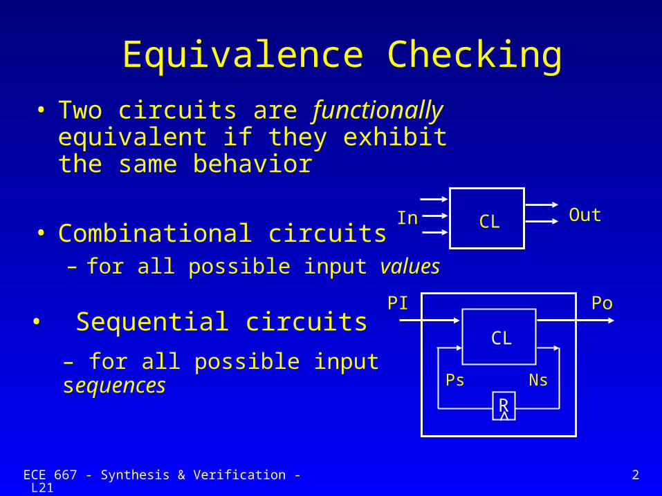
Equivalence Checking• Two circuits are functionally equivalent

if they exhibit the same behavior

• Combinational circuits – for all possible input values

In OutCL

PoPI

CL

Ps Ns

R

• Sequential circuits

– for all possible input sequences


Combinational Equivalence Checking

• Functional Approach– transform output functions of combinational

circuits into a unique (canonical) representation– two circuits are equivalent if their representations

are identical– efficient canonical representation: BDD

• Structural – identify structurally similar internal points– prove internal points (cut-points) equivalent– find implications


Functional Equivalence

• Circuits for which BDD can be constructed– represent multi-output circuits as shared BDDs– BDDs must be identical (for the same variable

ordering)

• Circuits whose BDDs are too large– cannot construct BDDs, memory problem– use partitioned BDD method

• decompose circuit into smaller pieces, each as BDD• check equivalence of internal points


Functional Decomposition

• Decompose each function into functional blocks– represent each block as a BDD (partitioned BDD method)– define cut-points (z)– verify equivalence of blocks at cut-points

starting at primary inputsF

f2

f1

z

x y

G

g2

g1

z

x y


Cut-Points Resolution Problem

F

f2

f1

z1

x y

G

g2

g1

z2

x y

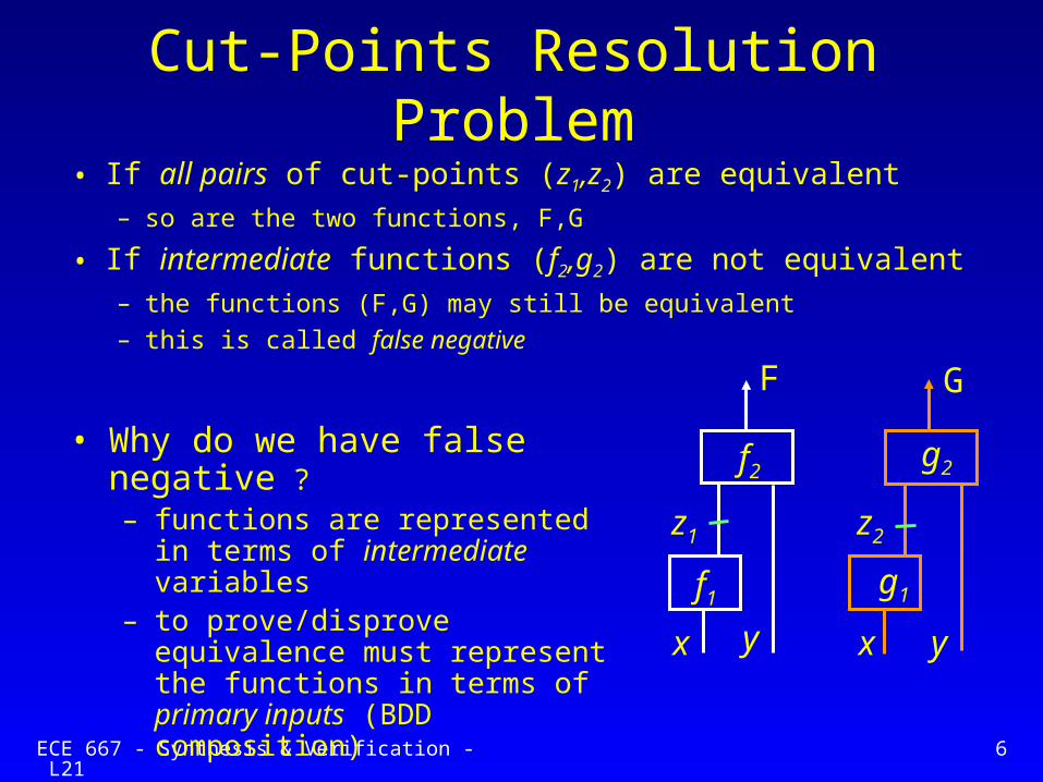
• If all pairs of cut-points (z1,z2) are equivalent– so are the two functions, F,G

• If intermediate functions (f2,g2) are not equivalent– the functions (F,G) may still be equivalent – this is called false negative

• Why do we have false negative ?– functions are represented in terms of

intermediate variables– to prove/disprove equivalence must

represent the functions in terms of primary inputs (BDD composition)


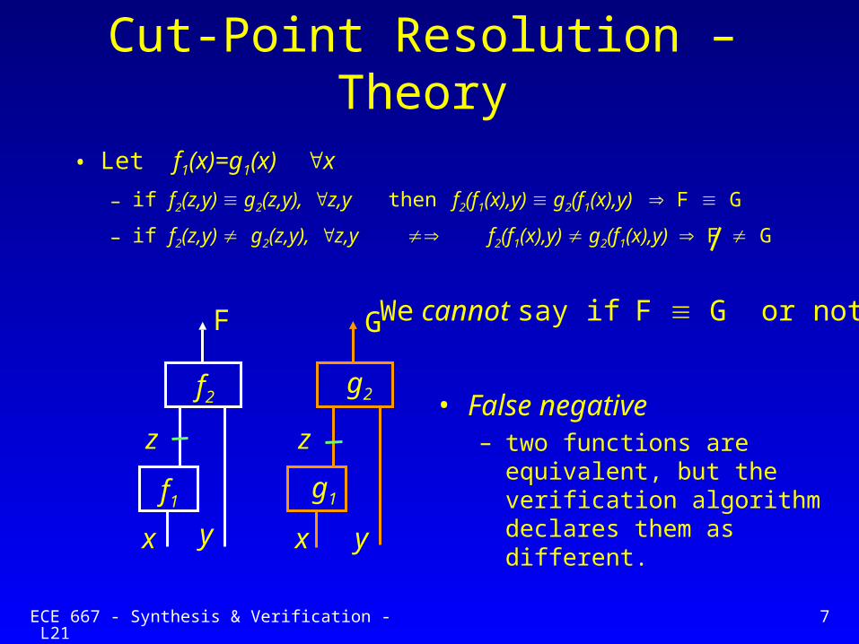
Cut-Point Resolution – Theory

• Let f1(x)=g1(x) x

– if f2(z,y) g2(z,y), z,y then f2(f1(x),y) g2(f1(x),y) F G

– if f2(z,y) g2(z,y), z,y f2(f1(x),y) g2(f1(x),y) F G

• False negative– two functions are equivalent,

but the verification algorithm declares them as different.

F

f2

f1

z

x y

G

g2

g1

z

x y

We cannot say if F G or not


Cut-Point Resolution – cont’d

• Procedure 1: create a miter (XOR) between

two potentially equivalent nodes/functions – perform ATPG test for stuck-at 0– find test pattern to prove F G

– efficient for true negative

(gives test vector, a proof)– inefficient when there is no test

0, F G (false negative) 1, F G (true negative)

F G

• How to verify if negative is false or true ?


Cut-Point Resolution – cont’d• Procedure 2: create a BDD for F G

– perform satisfiability analysis (SAT) of the BDD• if BDD for F G = , problem is not satisfiable, false negative• BDD for F G , problem is satisfiable, true negative

Non-empty, F G

, F G (false negative)F G =

=

F G

Note: must compose BDDs until they are equivalent, or expressed in terms of primary inputs

– the SAT solution, if exists, provides a test vector (proof of non-equivalence) – as in ATPG

– unlike the ATPG technique, it is effective for false negative (the BDD is empty!)


Structural Equivalence Check

• Given two circuits, each with its own structure– identify “similar” internal points, cut sets– exploit internal equivalences

• False negative problem may arise– F G, but differ structurally (different local support)– verification algorithm declares F,G as different

• Solution: use BDD-based or ATPG-based methods to resolve the problem. Also: implication, learning techniques.

b

d1a•

F a

c

d2

b •G


Implication Techniques

• Techniques that extract and exploit internal correspondences to speed up verification

• Implications – direct and indirect

a=1

c=x

b=xf=0

d=0

e=0

a=0

c=x

b=xf=1

d=x

e=x

Direct: a=1 f=0 Indirect (learning): f=1 a=0


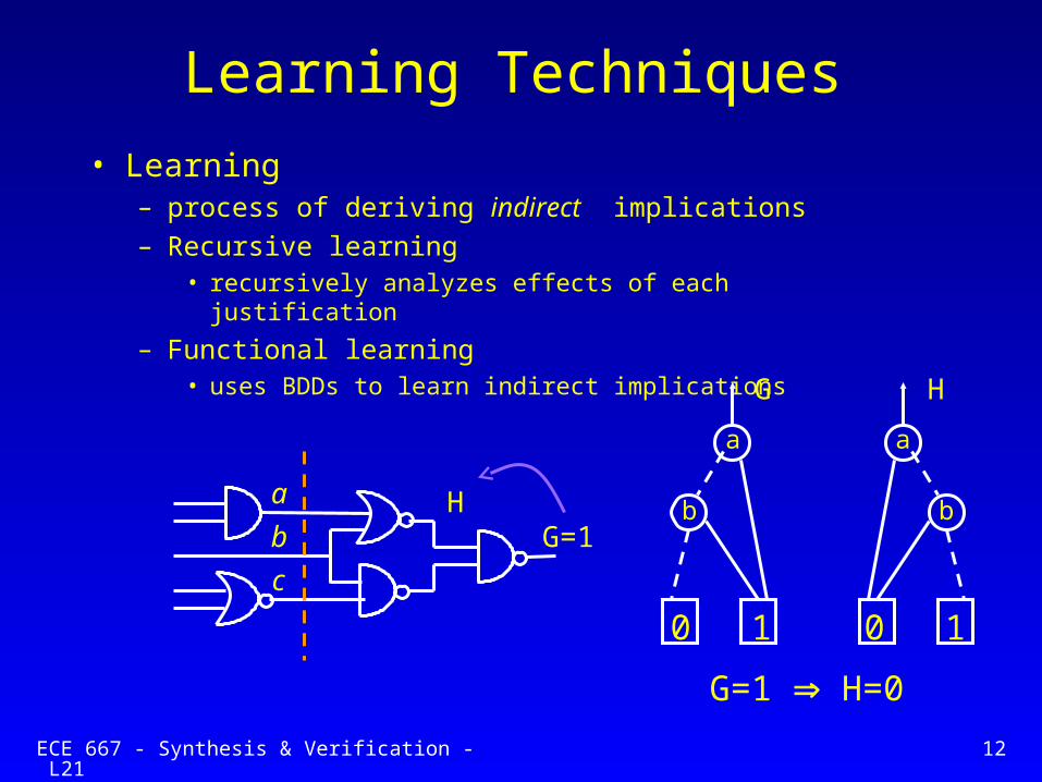
Learning Techniques

• Learning– process of deriving indirect implications– Recursive learning

• recursively analyzes effects of each justification

– Functional learning• uses BDDs to learn indirect implications

0 1

a

b

G

10

a

b

H

G=1 H=0

a

c

bH

G=1


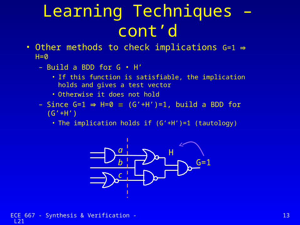
Learning Techniques –cont’d

• Other methods to check implications G=1 H=0

– Build a BDD for G • H’• If this function is satisfiable, the implication holds and

gives a test vector

• Otherwise it does not hold

– Since G=1 H=0 (G’+H’)=1, build a BDD for (G’+H’)• The implication holds if (G’+H’)=1 (tautology)

a

c

bH

G=1


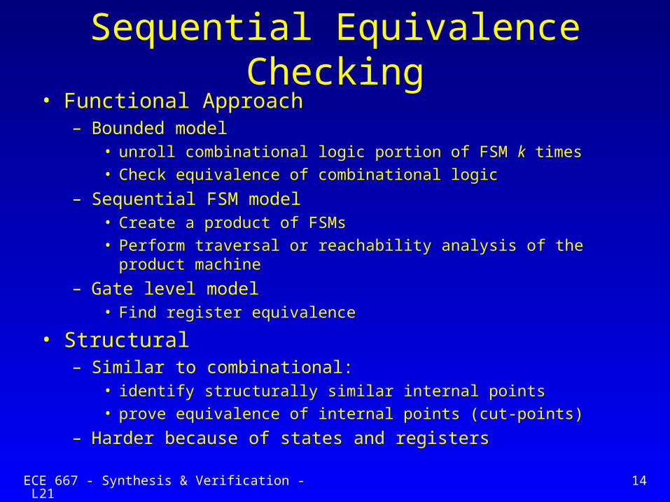
Sequential Equivalence Checking• Functional Approach

– Bounded model • unroll combinational logic portion of FSM k times

• Check equivalence of combinational logic

– Sequential FSM model• Create a product of FSMs

• Perform traversal or reachability analysis of the product machine

– Gate level model• Find register equivalence

• Structural – Similar to combinational:

• identify structurally similar internal points

• prove equivalence of internal points (cut-points)

– Harder because of states and registers


Finite State Machines (FSM)

• FSM M(X,S, , ,O)

– Inputs: X

– Outputs: O

– States: S

– Next state function, (s,x) : S X S

– Output function, (s,x) : S X O

OOXX

R

(s,x)(s,x)

s s’


Sequential Equivalence Checking• Represent each sequential circuit as an FSM

– verify if two FSMs are equivalent

• Approach 1: reduction to combinational circuit– unroll FSM over n time frames (flatten the design)

M(t1)

x(1)

s(1)

M(t2)

x(2)

s(2)…… M(tn)

x(n)

s(n)

Combinational logic: F(x(1,2, …n), s(1,2, … n))

– check equivalence of the resulting combinational circuits

– problem: the resulting circuit can be too large too handle


Sequential Verification

• Approach 2: based on isomorphism of state transition graphs– two machines M1, M2 are equivalent if their state transition

graphs (STGs) are isomorphic– perform state minimization of each machine– check if STG(M1) and STG(M2) are isomorphic

State min.1/0

0 1.20/0

1/1

0/1

M1min

1/0

0 10/0

1/1

0/1

M2

0/0 0/1

1/0

0 1

0/12

1/0

M1

1/1


Sequential Verification

• Approach 3: symbolic FSM traversal of the product machine

M1 M2S1 S2

O2O1

X

O(M)• Given two FSMs: M1(X,S1, 1, 1,O1), M2(X,S2, 2, 2,O2)

• Create a product FSM: M = M1 M2

– traverse the states of M and check its output for each transition

– the output O(M) =1, if outputs O1= O2

– if all outputs of M are 1, M1 and M2 are equivalent

– otherwise, an error state is reached

– error trace is produced to show: M1 M2


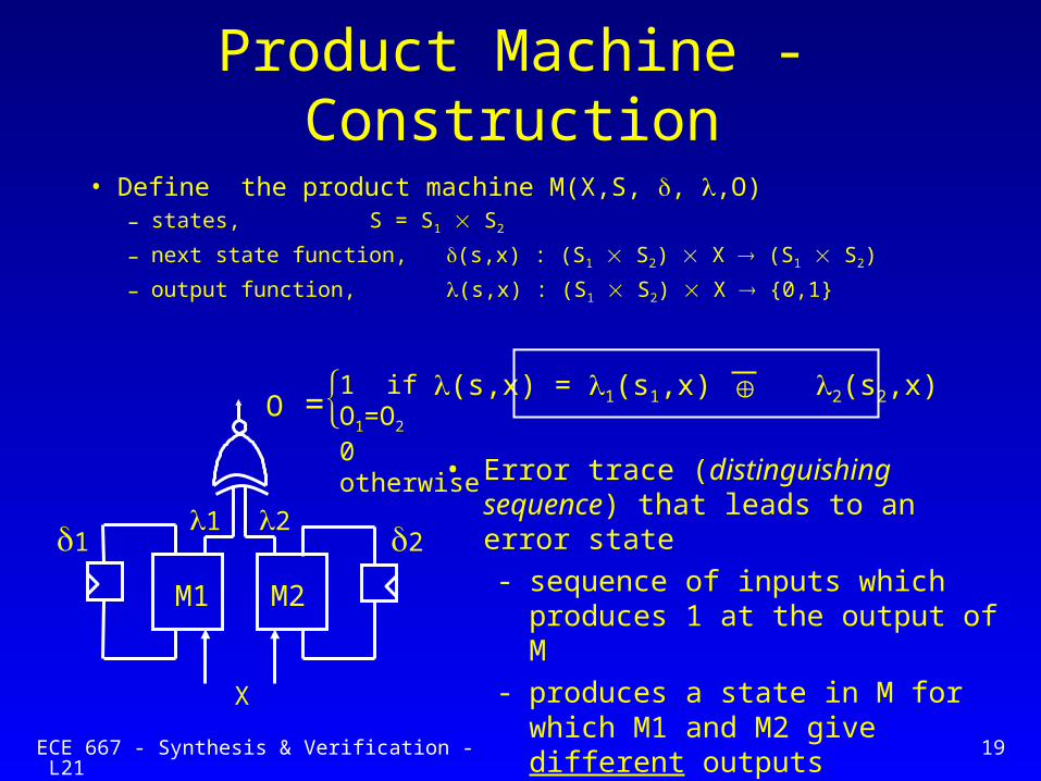
Product Machine - Construction

• Define the product machine M(X,S, , ,O)– states, S = S1 S2

– next state function, (s,x) : (S1 S2) X (S1 S2)

– output function, (s,x) : (S1 S2) X {0,1}

M1 M2

1 221

X

• Error trace (distinguishing sequence) that leads to an error state- sequence of inputs which produces 1

at the output of M - produces a state in M for which M1

and M2 give different outputs

(s,x) = 1(s1,x) 2(s2,x) O =1 if O1=O2

0 otherwise


Construction of the Product FSM

• For each pair of states, s1 M1, s2 M2

– create a combined state s = (s1. s2) of M– create transitions out of this state to other states of M– label the transitions (input/output) accordingly

1/0

0 10/0

1/1

0/1M1M2

1/1

2

0 10/0

0/0

0/11/1 1/0

M1

1/0

0

0/1

1

M2 2

0/1

1/01

1.1

0/100

1/10.2

11Output = {1 OK

0 error


(Explicit) FSM Traversal in Action

• STOP - backtrack to initial state to get error trace: x={1,1,1,0}

1/0

0 10/0

1/1

0/1

M1 M2

2

0 10/0

0/0

0/1

1/1

1/1 1/0

1.10/1

1/1

0/1

0.2

1/1

1.0 0/01/0

0/0 1.2

1/0

0.1

1/0

0/0 Out(M)State reached x=0 x=1

Error state

0.00/1 1/1M

Initiall states: s1=0, s2=0,s=(0.0)

• New 0 = (0.0) 1 1

• New 1 = (1.1) 1 1

• New 2 = (0.2) 1 1• New 3 = (1.0) 0 0


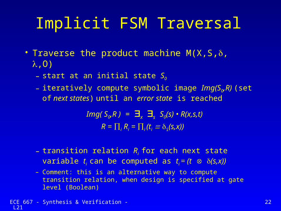
Implicit FSM Traversal

• Traverse the product machine M(X,S,, ,O)– start at an initial state S0

– iteratively compute symbolic image Img(S0,R) (set of next states) until an error state is reached

Img( S0,R ) = x s S0(s) • R(x,s,t)

R = i Ri = i (ti i(s,x))

– transition relation Ri for each next state variable ti

can be computed as ti = (t (s,x)) – Comment: this is an alternative way to compute transition

relation, when design is specified at gate level (Boolean)


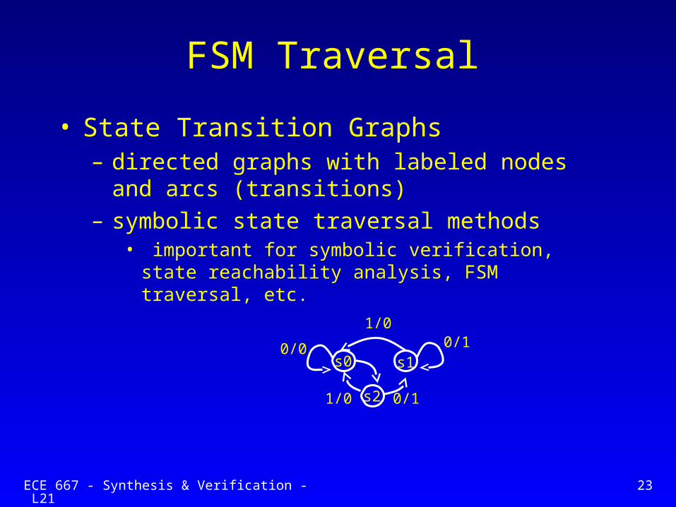
FSM Traversal

• State Transition Graphs – directed graphs with labeled nodes and arcs

(transitions)– symbolic state traversal methods

• important for symbolic verification, state reachability analysis, FSM traversal, etc.

0/0 0/1

1/0

s0 s1

0/1s2

1/0


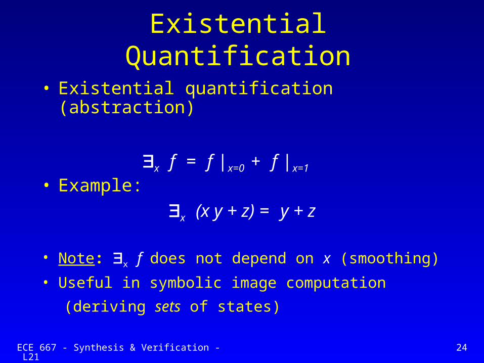
Existential Quantification

• Existential quantification (abstraction)

x f = f |x=0 + f |x=1

• Example:

x (x y + z) = y + z

• Note: x f does not depend on x (smoothing)

• Useful in symbolic image computation

(deriving sets of states)


Existential Quantification - cont’d

• Function can be existentially quantified w.r.to a vector: X = x1x2…

X f = x1x2... f = x1 x2 ... f

• Can be done efficiently directly on a BDD

• Very useful in computing sets of states – Image computation: next states

– Pre-Image computation: previous states

from a given set of initial states


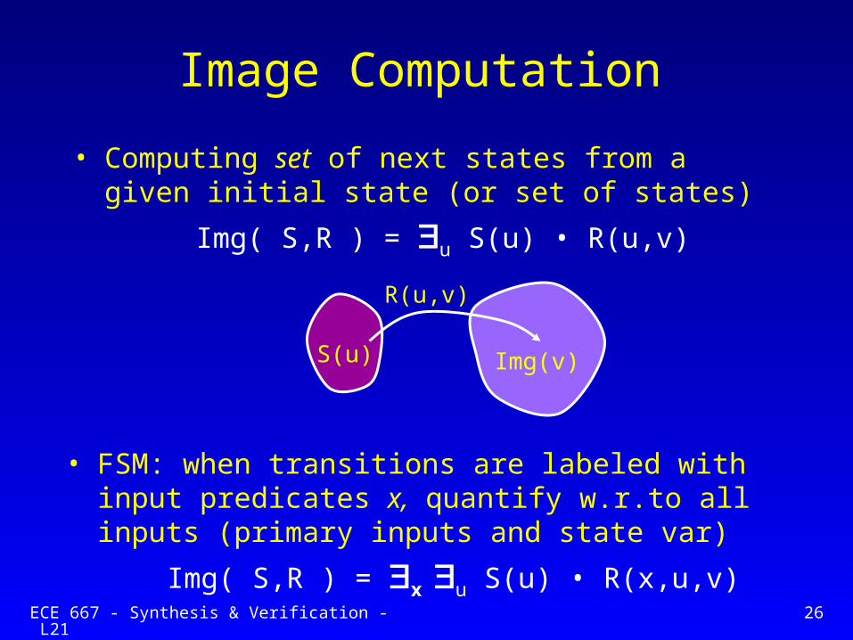
Image Computation

• Computing set of next states from a given initial state (or set of states)

Img( S,R ) = u S(u) • R(u,v)

Img(v)

R(u,v)

S(u)

• FSM: when transitions are labeled with input predicates x, quantify w.r.to all inputs (primary inputs and state var)

Img( S,R ) = x u S(u) • R(x,u,v)


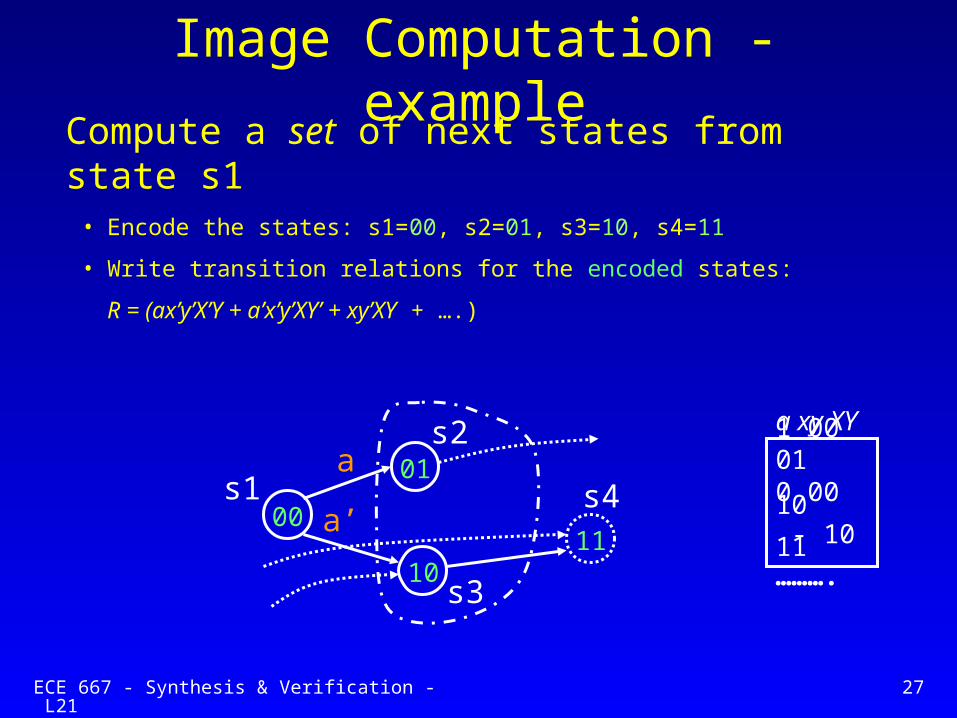
Image Computation - example

• Encode the states: s1=00, s2=01, s3=10, s4=11

• Write transition relations for the encoded states:

R = (ax’y’X’Y + a’x’y’XY’ + xy’XY + ….)

a xy XY1 00 010 00 10 - 10 11……….

s1

s2

s3

s4a

a’00

01

1011

Compute a set of next states from state s1


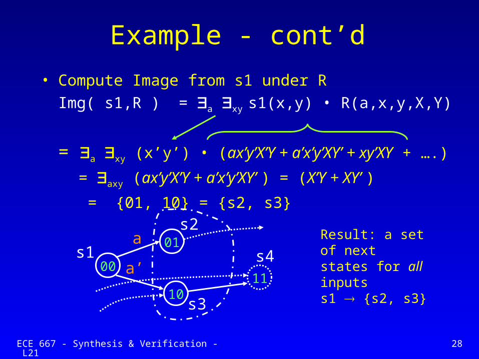
Example - cont’d

• Compute Image from s1 under R

Img( s1,R ) = a xy s1(x,y) • R(a,x,y,X,Y)

= a xy (x’y’) • (ax’y’X’Y + a’x’y’XY’ + xy’XY + ….)

= axy (ax’y’X’Y + a’x’y’XY’ ) = (X’Y + XY’ )

= {01, 10} = {s2, s3}

Result: a set of next states for all inputs s1 {s2, s3}

s1

s2

s3

s4a

a’00

01

1011


Pre-Image Computation

• Computing a set of present states from a given next state (or set of states)

Pre-Img( S’,R) = v R(u,v) )• S’(v)

S’(v)

R(u,v)

Pre-Img(u)

• Similar to Image computation, except that quantification is done w.r.to next state variables

• The result: a set of states backward reachable from state set S’, expressed in present state variables u

• Useful in computing CTL formulas: AF, EF

ece 667 - synthesis & verification - l211 ece 697b (667) spring 2006 synthesis and verification...

Documents