eccv 2010 - mitsubishi electric research laboratories october 2010 ... lead to conic epipolar...

MITSUBISHI ELECTRIC RESEARCH LABORATORIEShttp://www.merl.com

Analytical Forward Projection for AxialNon-Central Dioptric & Catadioptric

Cameras

Amit Agrawal, Yuichi Taguchi, Srikumar Ramalingam

TR2010-081 October 2010

Abstract

We present a technique for modeling non-central catadioptric cameras consisting of a perspectivecamera and a rotationally symmetric conic reflector. While previous approaches use a central ap-proximation and/or iterative methods for forward projection, we present an analytical solution.This allows computation of the optical path from a given 3D point to the given viewpoint by solv-ing a 6th degree forward projection equation for general conic mirrors. For a spherical mirror,the forward projection reduces to a 4th degree equation, resulting in a closed form solution. Wealso derive the forward projection equation for imaging through a refractive sphere (non-centraldioptric camera) and show that it is a 10th degree equation. While central catadioptric cameraslead to conic epipolar curves, we show the existence of a quartic epipolar curve for catadioptricsystems using a spherical mirror. The analytical forward projection leads to accurate and fast 3Dreconstruction via bundle adjustment. Simulations and real results on single image sparse 3Dreconstruction are presented. We demonstrate 100 times speed up using the analytical solutionover iterative forward projection for 3D reconstruction using spherical mirrors.

ECCV 2010

This work may not be copied or reproduced in whole or in part for any commercial purpose. Permission to copy in whole or in partwithout payment of fee is granted for nonprofit educational and research purposes provided that all such whole or partial copies includethe following: a notice that such copying is by permission of Mitsubishi Electric Research Laboratories, Inc.; an acknowledgment ofthe authors and individual contributions to the work; and all applicable portions of the copyright notice. Copying, reproduction, orrepublishing for any other purpose shall require a license with payment of fee to Mitsubishi Electric Research Laboratories, Inc. Allrights reserved.

Copyright c©Mitsubishi Electric Research Laboratories, Inc., 2010201 Broadway, Cambridge, Massachusetts 02139

MERLCoverPageSide2

Analytical Forward Projection for Axial

Non-Central Dioptric & Catadioptric Cameras

Amit Agrawal, Yuichi Taguchi, and Srikumar Ramalingam

Mitsubishi Electric Research Labs (MERL), Cambridge, MA, USA

Abstract. We present a technique for modeling non-central catadioptriccameras consisting of a perspective camera and a rotationally symmetricconic reflector. While previous approaches use a central approximationand/or iterative methods for forward projection, we present an analyt-ical solution. This allows computation of the optical path from a given3D point to the given viewpoint by solving a 6th degree forward pro-jection equation for general conic mirrors. For a spherical mirror, theforward projection reduces to a 4th degree equation, resulting in a closedform solution. We also derive the forward projection equation for imag-ing through a refractive sphere (non-central dioptric camera) and showthat it is a 10th degree equation. While central catadioptric cameraslead to conic epipolar curves, we show the existence of a quartic epipolarcurve for catadioptric systems using a spherical mirror. The analyti-cal forward projection leads to accurate and fast 3D reconstruction viabundle adjustment. Simulations and real results on single image sparse3D reconstruction are presented. We demonstrate ∼ 100 times speedup using the analytical solution over iterative forward projection for 3Dreconstruction using spherical mirrors.

1 Introduction

Catadioptric cameras allow large field of view 3D reconstruction and stable ego-motion estimation from few images. As analyzed in [1], there are only a fewconfigurations that allow an effective single-viewpoint (central) catadioptric sys-tem. Simple mirrors such as sphere as well as configurations when the camerais not placed on the foci of hyperbolic/elliptical mirrors lead to a non-centralsystem. To handle such configurations, it is important to accurately model a non-cental catadioptric camera. Approximations using a central model could lead toinaccuracies such as skewed 3D estimation [2].

The projection of a scene point onto the image plane (Forward Projection)requires computing the light path from the scene point to the perspective cam-era’s center of projection (COP). Thus, the reflection point on the mirror needsto be determined. This is considered to be hard problem and iterative solutionsare usually employed assuming there are no closed form solutions. In this paper,we present an analytical solution to compute the forward projection (FP) forconic catadioptric systems, where the mirror is obtained by revolving a conicsection around the axis of symmetry and the camera’s COP is placed on the

2 Amit Agrawal, Yuichi Taguchi, Srikumar Ramalingam

mirror axis. We show that for a given 3D point, the mirror reflection point canbe obtained by solving a 6th degree equation for a general conic mirror. Interest-ingly, it reduces to solving a 4th degree equation for a spherical mirror, resultingin a closed form solution. We show how to use these analytical solutions for fast3D reconstruction using bundle adjustment, achieving a two order of magnitudespeed up over previous approach [2].

Forward projection for imaging through a refractive sphere (non-central diop-tric camera) is even more challenging due to two refractions. We show that theoptical path from a given 3D point to a given viewpoint via a refractive spherecan be obtained by solving a 10th degree equation. Thus, similar to mirrors,refractive spheres can also be used for 3D reconstruction by plugging its forwardprojection equation in a bundle adjustment algorithm. We believe that ours isthe first paper to analyze this problem and derive a practical solution.

The epipolar geometry for central catadioptric systems (CCS) and for severalnon-central cameras (pushbroom, cross-slit, etc.) has been extensively studied.However, analyzing the epipolar geometry for non-central catadioptric camerasis difficult due to non-linear forward projection. We show the existence of aquartic epipolar curve for catadioptric systems employing spherical mirror.Contributions: Our paper makes the following contributions:

– We analyze forward projection for axial non-central dioptric/catadioptriccameras with conic reflectors and refractive spheres, and show that analyticalsolutions exist.

– We demonstrate that the back-projection for a spherical mirror can be for-mulated as a matrix-vector product and that the corresponding epipolarcurves are quartic.

– We utilize the forward projection equations for fast sparse 3D reconstruction.

1.1 Related Work

Back-Projection and Epipolar Geometry: Baker and Nayar [1] presentedthe complete class of central catadioptric systems. Svoboda et al. [3, 4] studiedthe epipolar geometry for CCS and showed that the epipolar curves are conics.Geyer and Daniilidis [5] showed the existence of fundamental matrix for para-catadioptric cameras. A unified imaging model for all CCS was proposed byGeyer and Daniilidis [6]. Using this model for forward/back-projection with sec-ond order lifted image coordinates, Strum and Barreto [7] formulated the funda-mental matrix for all CCS. For non-central cameras, Pless [8] introduced essentialmatrix for the calibrated case. Rademacher and Bishop [9] described epipolarcurves for arbitrary non-central images. The epipolar geometry of cone-shapedmirrors, when restricted to planar motions was derived by Yagi and Kawato [10].Spacek [11] described the epipolar geometry for two cameras mounted one ontop of the other with aligned mirror axes.

Representing back-projection as a matrix-vector product for general mir-rors is typically difficult. Several non-central cameras can be modeled by back-projection matrices operating on second order lifted image coordinates, result-

Analytical Forward Projection for Axial Non-Central Cameras 3

ing in conic epipolar curves. These include linear pushbroom cameras [12], lin-ear oblique cameras [13], para-catadioptric cameras [14], and all general linearcameras (GLC) [15]. For the one-coefficient classical radial distortion model, theepipolar curves are cubic [16]. We show that for spherical mirror, back-projectioncan be described as matrix-vector product using fourth order lifted image coor-dinates, and thus the epipolar curves are quartic.Forward projection for a non-central catadioptric camera is a hard problem,since the point on the mirror where the reflection happens need to be determined.In general, there is no closed-form solution for this problem, so non-linear opti-mization have been proposed (as in [17, 2]). Goncalves and Nogueira [18] inves-tigated quadric-shaped mirrors and reduced the problem to an optimization ina single variable. Baker and Nayar [1] were unable to find a closed form solutionwhile analyzing mirror defocus blur and used numerical solutions. Their analysiswas in 3D, since the finite camera aperture requires considering viewpoints noton the mirror axis. Vandeportaele [19] also analyzed forward projection for axialcase, but in 3D using intersection of quadrics. In contrast, we derive a muchsimpler solution for the axial case in 2D with lower degree equation comparedto [19].Spherical mirrors have been used for visual servoing and wide-angle 3D re-construction [20–22, 17, 2, 23]. Both [22] and [2] state that computing forwardprojection does not have a closed-form solution. In [22], a GLC approximationis used by tessellating the captured multi-perspective image into triangles andassociating a GLC with each of them. In [2], an iterative method for forwardprojection is used. Interestingly, for spherical mirror, forward projection corre-sponds to the classical Alhazen’s problem with four solutions [24]. We show thatour FP equation for general quadric mirror reduces to a 4th order equation forspherical mirror. Garg and Nayar [25] used a refractive sphere model for raindrops for generating near-perspective images (environment at infinity). However,they did not solve for the forward projection from a 3D point to compute theoptical path, which we describe.

2 Forward Projection: Conic Reflectors

We first derive the forward projection equation for conic catadioptric systems.Let z axis be the mirror axis. A pinhole camera is placed at a distance d fromthe origin on the mirror axis. Let P = [X,Y, Z]

Tbe a 3D scene point. Since the

mirror is rotationally symmetric, the mirror reflection of P can be analyzed inthe plane π containing the mirror axis and P (Figure 1 (left)). Let (z1, z2) be

the local coordinate system of π. In this plane, P has coordinates p = [u, v]T

given by u = S sin θ and v = Z, where S =√X2 + Y 2 + Z2 is the distance of

P from the origin and θ = cos−1(Z/S) is the angle between the mirror axis andthe line joining the origin and the 3D point.

In plane π, the mirror is parameterized as a 2D conic Az22 + z21 + Bz2 = C.This parametrization is used in [26] to handle spherical mirror along with other

mirrors for computing the caustics. Let m = [x, y]Tbe the reflection point on the


Refractive sphere

COP (0, d)

p (u, v)

v1

n1 (x, y)

n2 (x2, y2)

v2

α

α

β

β

v3

Conic catadioptric system Refractive sphere

Plane π

Mirror profile

COP (0, d)

m (x, y)

p (u, v)

z2

vi

vr

n

z1x

y

P (X, Y, Z)

Mirror surface

COP(0, 0, d)

Plane π

z: Mirror axis

θ

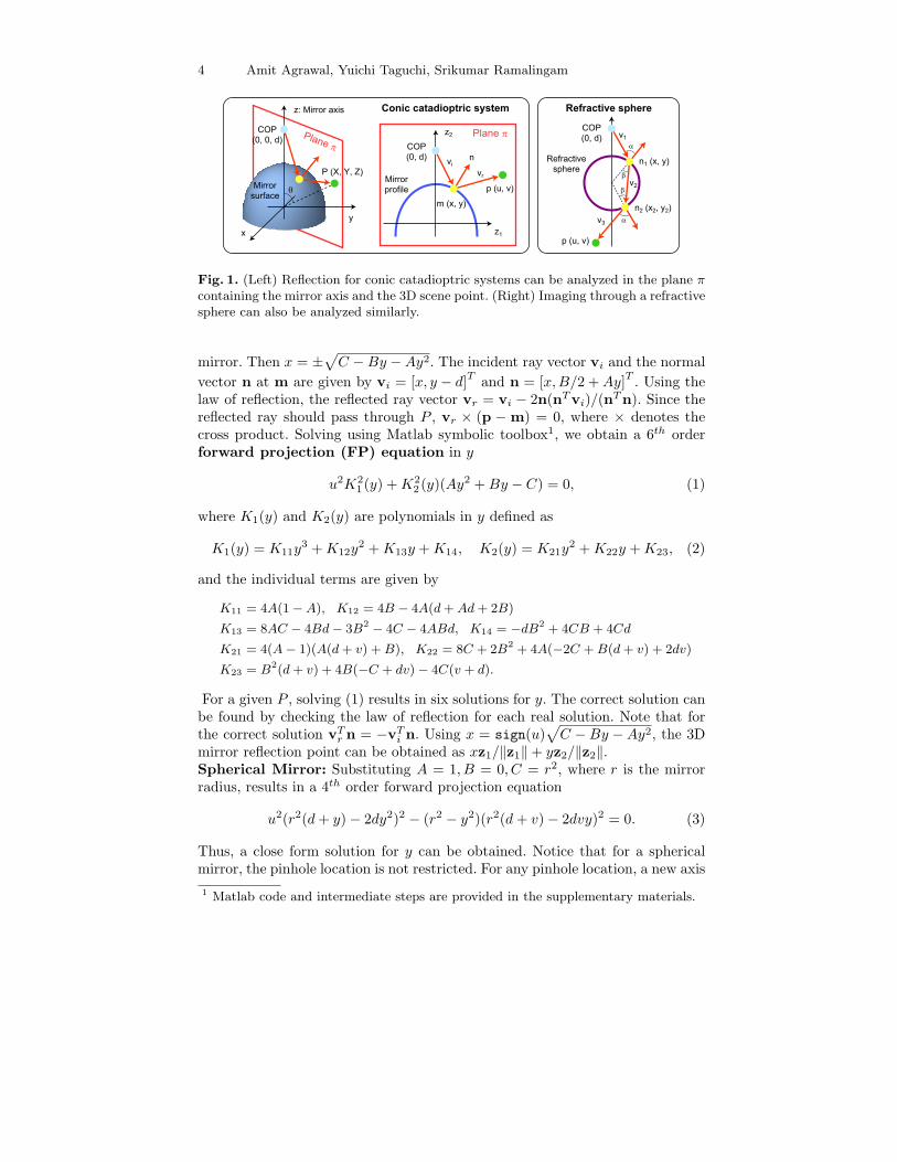
Fig. 1. (Left) Reflection for conic catadioptric systems can be analyzed in the plane πcontaining the mirror axis and the 3D scene point. (Right) Imaging through a refractivesphere can also be analyzed similarly.

mirror. Then x = ±√

C −By −Ay2. The incident ray vector vi and the normal

vector n at m are given by vi = [x, y − d]Tand n = [x,B/2 +Ay]

T. Using the

law of reflection, the reflected ray vector vr = vi − 2n(nTvi)/(nTn). Since the

reflected ray should pass through P , vr × (p − m) = 0, where × denotes thecross product. Solving using Matlab symbolic toolbox1, we obtain a 6th orderforward projection (FP) equation in y

u2K21 (y) +K2

2 (y)(Ay2 +By − C) = 0, (1)

where K1(y) and K2(y) are polynomials in y defined as

K1(y) = K11y3 +K12y

2 +K13y +K14, K2(y) = K21y2 +K22y +K23, (2)

and the individual terms are given by

K11 = 4A(1−A), K12 = 4B − 4A(d+Ad+ 2B)

K13 = 8AC − 4Bd− 3B2− 4C − 4ABd, K14 = −dB2 + 4CB + 4Cd

K21 = 4(A− 1)(A(d+ v) +B), K22 = 8C + 2B2 + 4A(−2C +B(d+ v) + 2dv)

K23 = B2(d+ v) + 4B(−C + dv)− 4C(v + d).

For a given P , solving (1) results in six solutions for y. The correct solution canbe found by checking the law of reflection for each real solution. Note that forthe correct solution vT

r n = −vTi n. Using x = sign(u)

√

C −By −Ay2, the 3Dmirror reflection point can be obtained as xz1/‖z1‖+ yz2/‖z2‖.Spherical Mirror: Substituting A = 1, B = 0, C = r2, where r is the mirrorradius, results in a 4th order forward projection equation

u2(r2(d+ y)− 2dy2)2 − (r2 − y2)(r2(d+ v)− 2dvy)2 = 0. (3)

Thus, a close form solution for y can be obtained. Notice that for a sphericalmirror, the pinhole location is not restricted. For any pinhole location, a new axis

1 Matlab code and intermediate steps are provided in the supplementary materials.


Table 1. Degree of forward projection equation for central and non-central catadioptricsystems using conic reflectors.

Mirror Shape Pinhole Placement Parameters Central System Degree

General On axis A,B,C No 6Sphere Any A = 1, B = 0, C > 0 No 4Elliptic On axis, At Foci B = 0 Yes 2Elliptic On axis, Not at Foci B = 0 No 6

Hyperbolic On axis, At Foci A < 0, C < 0 Yes 2Hyperbolic On axis, Not at Foci A < 0, C < 0 No 6Parabolic On axis, d = ∞ A = 0, C = 0 Yes 2Parabolic On axis, Finite d A = 0, C = 0 No 5

joining the pinhole and the sphere center can be defined. In all other cases, thepinhole needs to be on the mirror axis. Table 1 shows the degree of FP equationfor spherical (A = 1, B = 0, C > 0), elliptical (B = 0), hyperbolic (A < 0, C < 0)and parabolic (A = 0, C = 0) mirrors. Note that when the catadioptric systemis central, the degree of FP is two. This is intuitive, since the reflection pointcan be obtained by intersecting the mirror with the ray joining the 3D point andthe effective projection center.

3 Back-Projection & Epipolar Curve for Spherical Mirror

Now we show that back-projection equations for a non-central catadioptric sys-tem using a spherical mirror can be written in matrix-vector form. By intersect-ing the back-projected ray with a general 3D ray, we show the existence of aquartic epipolar curve. Then we verify that the projection of points on the same3D line onto the image plane using the FP equation results in the same curve.

Let Cp = [0, 0,−d]T

be the COP and let the spherical mirror of radius rbe located at the origin (Figure 2 (left)). For an image point q, let s = K−1qbe the ray direction, where K3×3 is the internal camera calibration matrix. Theintersection points b with the mirror are given by

b = Cp + sds3 ±

√

d2s23 − (d2 − r2)(sT s)

sT s, (4)

where s3 is the third element of s. Note that bTb = r2 and the normal at b isb/r. Since vi = b−Cp, the reflected vector vr is given by

vr = (b−Cp)− 2b(bT (b−Cp))/r2 = −b−Cp + 2b(bTCp)/r

2, (5)

which intersects the mirror axis at m = [0, 0, k]T, where k = dr2/(2db3 + r2).

Thus, the Plucker coordinates of the reflected 3D ray are given by L = (bT −mT , (b×m)T )T , where × denotes the cross product. Similar to [7], we use L+

and L− to represent the reflected rays corresponding to the two intersections of


Cp (0, 0, -d)

b−

m−

b+m+

L−

L+

O

s

q

b+

Spherical

mirror

−0.06 −0.04 −0.02 0 0.02 0.04 0.06

−0.06

−0.04

−0.02

0

0.02

0.04

0.06

Nomalized Image Coordinate x

No

rma

lize

d Im

ag

e C

oo

rdin

ate

y (a) Analytical

Epipolar Curve

(b) Using Forward

Projection

Sphere

Boundary

Fig. 2. (Left) Depicting back-projection. (Right) Epipolar curves, analytically com-puted by Equation (8) (a) and numerically computed by using the FP equation (b) fora known 3D line match.

vi with the sphere (b+ and b−). We represent the two lines with a second-orderline complex C, described as a symmetric 6× 6 matrix

C ∼ W (L+LT− + L−L

T+)W, W =

(

0 II 0

)

, (6)

where ∼ denotes the equality of matrices up to a scale factor. By substitutingb and m, we obtain a line complex C that includes quartic monomials of s. Asin [7], let vsym(C) be the column-wise vectorization of the upper-right trian-

gular part of C (21-vector) and ˆs denote double lifted coordinates of s in thelexicographic order (15-vector). Then we obtain the back-projection equation ina matrix-vector form:

vsym(C) ∼ Br,dˆs = Br,d

ˆK−1 ˆq, (7)

where Br,d is a sparse 21 × 15 matrix depending only on r and d, as shown inthe supplementary materials.

Note that the difference between [7] and ours is that m = [0, 0, 0] in [7], sincethe reflected ray passes through the center of an imaginary sphere that modelsall central catadioptric systems [6]. For a non-central catadioptric system, mbecomes dependent on the image pixel q. Note that when the pinhole is on themirror axis, one can always find the intersection point m as [0, 0, k] for some k.Epipolar Curve: Consider a 3D ray defined in the sphere-centered coordinatesystem and represented with Plucker coordinates as L0. This ray intersects theline complex C iff

LT0 CL0 = 0. (8)

Since C includes quartic monomials of s (thus q), the constraint results in a4th order curve. The projection of L0 therefore appears as a quartic curve in theimage of spherical mirror, which means that spherical-mirror based catadioptricsystems yield quartic epipolar curves. Our FP equation allows us to validate the


degree and shape of epipolar curves. Figure 2 (right) compares the epipolar curveanalytically computed from (8) with the curve obtained by projecting 3D pointson L0 using the FP equation. We can observe that the shape of curves agree andthe numerical curve (using FP) is a continuous section of the analytical quarticcurve. Note that the image point converges as the 3D point goes to ±∞ on L0.

Similar to perspective cameras, the quartic epipolar curve can be used to re-strict the search space for dense stereo matching. Typically, approximations suchas epsilon-stereo constraint [22] are used, which assumes that the correspondingmatch will lie approximately along a line. However, our analysis provides theanalytical 2D epipolar curve for non-central spherical mirror cameras. Note thatthe FP equation for general conic mirrors simplifies the correspondence searchfor other non-central conic catadioptric systems as well.

4 Sparse 3D Reconstruction using Spherical Mirrors

We demonstrate the applicability of analytical forward projection (AFP) forsparse 3D reconstruction using well-known bundle adjustment algorithm, andcompare it with iterative forward projection (IFP) method [2]. We choose asimpler setup of a single perspective camera imaging multiple spherical mirrorsas shown in Figure 4. We assume that the internal camera calibration is doneseparately (off-line) and the sphere radius is known (we used high sphericitystainless steel balls as spherical mirrors for real experiments). Thus, our opti-mization involves estimating the sphere centers and the 3D points in the cameracoordinate system. Note that the FP equation can be easily applied to more gen-eral calibration/3D reconstruction involving rotationally symmetric setups withparabolic/hyperbolic mirrors [2]. For moving camera+mirror system, one mayrequire a central approximation to get the initial estimate of the relative cameramotion. However, AFP can replace IFP in subsequent bundle adjustment. Inaddition, since AFP leads to a fast algorithm, we demonstrate in Section 4.3that a central approximation is not required for iterative outlier removal.

4.1 Bundle Adjustment for Spherical Mirror using AFP

Let C(i) =[

Cx(i), Cy(i), Cz(i)]T

, i = 1 . . .M be the sphere centers and P(j) =[

Px(j), Py(j), Pz(j)]T

, j = 1 . . . N be the 3D points in the camera coordinatesystem, when the pinhole camera is placed at the origin. First we rewrite the FPequation (3) in terms of 3D quantities. For a given 3D point P(j) and mirrorcenter C(i), the orthogonal vectors z1 and z2 defining plane π are given by

z2 = −C(i) and z1 = P(j) − C(i)C(i)TP(j)‖C(i)‖2 . Further, d = ‖z2‖, u = ‖z1‖, and

v = −C(i)T (P(j) − C(i))/‖C(i)‖. By substituting d, u and v in (3), the FPequation can be re-written as

c1y4 + c2y

3 + c3y2 + c4y + c5 = 0, (9)

where each coefficient ci becomes a function of P(j) and C(i) only. In general,when the scene point is outside the sphere and is visible through mirror reflection,


there are four real solutions. The single correct solution is found by checking thelaw of reflection for each of them.

Using the solution, the 3D reflection point on the sphere is obtained as

Rm(i, j) = [Xm(i, j), Ym(i, j), Zm(i, j) ]T= C(i) +

√

r2 − y2z1

‖z1‖+ y

z2

‖z2‖. (10)

Finally, the 2D image projection pixel is obtained as p(i, j) = fxXm(i,j)Zm(i,j) + cx,

q(i, j) =fyYm(i,j)Zm(i,j) + cy, where (fx, fy) and (cx, cy) are the focal length and the

principal point of the camera, respectively.Let [p(i, j), q(i, j)]

Tbe the image projection of the jth 3D point for the ith

sphere and [p(i, j), q(i, j)]T

denote their current estimates, computed from thecurrent estimates of sphere centers and 3D scene points. Each pair (i, j) gives a

2-vector error function F (i, j) = [p(i, j)− p(i, j), q(i, j)− q(i, j)]T, and the aver-

age reprojection error is given by E = 1NM

∑Nj=1

∑Mi=1 ‖F (i, j)‖2. We perform

bundle adjustment by minimizing E (using Matlab function lsqnonlin), start-ing from an initial solution. The initial 3D points are obtained as the center ofthe shortest transversal of the respective back-projection rays. The initial spherecenters are perturbed from their true positions (simulations) and obtained usingthe captured photo (real experiments).Jacobian Computation: AFP also enables the analytical Jacobian computa-tion, which speeds up bundle adjustment. Let t denote an unknown. Then

∂F (i, j)

∂t=

[

∂p(i,j)∂t

∂q(i,j)∂t

]

=

[

fx(1

Zm(i,j)∂Xm(i,j)

∂t − Xm(i,j)Zm(i,j)2

∂Zm(i,j)∂t )

fy(1

Zm(i,j)∂Ym(i,j)

∂t − Ym(i,j)Zm(i,j)2

∂Zm(i,j)∂t )

]

. (11)

Since Xm, Ym, Zm depend on y, the above derivatives depend on ∂y∂t . Typically,

one would assume that a closed form expression for y is required to compute ∂y∂t .

However, it can be avoided by taking the derivative of the FP equation (9) as

∂y

∂t= −y4 ∂c1

∂t + y3 ∂c2∂t + y2 ∂c3

∂t + y ∂c4∂t + ∂c5

∂t

4c1y3 + 3c2y2 + 2c3y + c4. (12)

For a given 3D point P(j) and sphere center C(i), y can be computed by solvingthe FP equation and thus can be substituted in above to obtain ∂y

∂t . The gradientof the reprojection error with respect to each unknown can be obtained usingEquations (10),(11), and (12). Thus, we showed that the analytical FP equationcan be used to compute the Jacobian of the reprojection error, without obtaininga closed-form solution for the mirror reflection point.

4.2 Simulations

We place a pinhole camera at the center of the coordinate system and M = 4spheres (radius r = 0.5”) at a distance of 200 mm. N = 100 3D points were ran-domly distributed in a hemisphere of radius 1000 mm surrounding the spheres


0 0.2 0.4 0.6 0.8 10

1

2

3

Image Point Noise [pixel]

Repro

jection E

rror

[pix

el]

Ours

Central

2 Iterations

Full Iterations

0 0.2 0.4 0.6 0.8 10

100

200

300

400

500

600


RM

SE

of 3D

Poin

ts [m

m]

Initial

Ours

2 Iterations

Full Iterations

Fig. 3. Bundle adjustment simulations using M = 4 spherical mirrors and N = 1003D points for different image noise levels. (Left) Reprojection error. (Right) RMSEof reconstructed 3D points. The IFP curve matches the AFP curve when sufficientiterations are used.

Table 2. Comparison of bundle adjustment run time (in seconds) using IFP [2] andour AFP for N 3D points and M = 4 spherical mirrors. The run times were obtainedby repeating bundle adjustment 20 times and averaging.

Run Time Iterative FP AFP (Without Jacobian) AFP (With Jacobian)

N = 100 470 6.6 4.0N = 1000 4200 68 48

and their true image projections were computed using the FP equation. Gaussiannoise was added both to sphere centers (σ = 0.5 mm) and true image projec-tions (σ = [0 − 1] pixels). We compare the reconstruction error using (a) AFP,(b) central approximation (the projection center was fixed at 0.64r mm fromthe sphere center as in [2]), and (c) IFP [2]. IFP first computes the initial im-age projection of a 3D point using the central approximation and then performsnon-linear optimization to minimize the distance between the 3D point and theback-projected ray. It required ∼ 5 iterations to converge in the simulations.

Figure 3 compares the reprojection error and the root mean square error(RMSE) in 3D points for different image noise levels. Note that only when suf-ficient iterations are performed for IFP (referred to as ‘full iterations’), its errorreduces to that of AFP (same curve). The central approximation or smaller num-ber of iterations for IFP lead to larger errors. In Figure 3 (right), the error dueto central approximation is too large (1.5× 104 mm) to be shown in the graph.

Run time for projecting 105 3D points with a single sphere was 1120 secondsfor IFP (full iterations) and 13.8 seconds for AFP (∼ 80 times faster). Table 2compares the bundle adjustment run time, which shows that AFP along withanalytical Jacobian computation achieves a speed up of ∼ 100. While the numberof iterations in bundle adjustment was almost the same for IFP and AFP, IFPtakes much longer time due to iterative optical path computation for each 3Dpoint and mirror pair. Similar speed-ups were obtained for elliptic, hyperbolic,


Plane 1Plane 2

Plane 3

Plane 4

Plane 1Plane 2

Plane 3

Plane 4

Center

Le

ft

Rig

ht

Top

Bottom

Center

Le

ft

Rig

ht

Top

Bottom

Fig. 4. Input images (left) and zoom-in of sphere images (middle and right) superim-posed with extracted SIFT features. Red dots and green crosses respectively representinliers and outliers determined in the iterative bundle adjustment process. Top showsrendered image using POV-Ray and bottom shows real photo captured using a camera.

and parabolic mirrors as well (projecting 105 3D points took 1600–1800 secondsfor IFP and 22 seconds for AFP).

4.3 POV-Ray Simulations and Real Results using Feature Matching

In practice, the corresponding image points are estimated using a feature match-ing algorithm such as SIFT, and invariably contain outliers and false matches.We first show results using SIFT on sphere images rendered using POV-Ray,which allows performance evaluation using available ground truth data.

Figure 4 (top) shows a rendered image (resolution 2000×2000) of four spher-ical mirrors, placed at the center of a cube 1000mm on each side. The walls of thecube consist of textured planes. We extract SIFT features and select correspond-ing points that are consistent among the four sphere images. For initial spherecenters, we add Gaussian noise (σ = 0.3mm) to their ground truth locations.Since the SIFT matches contains outliers, we perform robust reconstruction byiterating bundle adjustment with outlier removal. After each bundle adjustmentstep, we remove all 3D points whose reprojection error is greater than twice theaverage reprojection error. Figure 5 shows that by iterating bundle adjustmentand outlier removal, the reprojection error and RMSE of 3D points reduces sig-nificantly for all planes (from ∼ 460 mm to 6 mm). Figure 5 also shows thenumber of inliers after each bundle adjustment step. Note that since AFP signif-icantly reduces bundle adjustment time, this simple procedure can be repeatedmultiple times and is effective in handling outliers.


0 2 4 6 8 100.1

0.2

0.3

0.4

0.5

Iterations (Bundle Adjustment/Outlier Removal)

Re

pro

jectio

n E

rro

r [p

ixe

ls]

0 2 4 6 8 100

200

400

600

800


Err

or

fro

m G

T P

lan

e [

mm

]

Center PlaneRight PlaneLeft PlaneTop PlaneBottom Plane

0 2 4 6 8 10480

500

520

540

560

580

600


Nu

mb

er

of

Inlie

rs

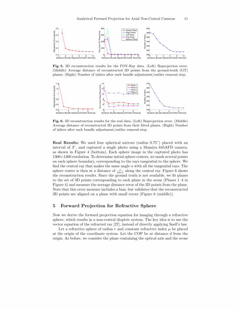
Fig. 5. 3D reconstruction results for the POV-Ray data. (Left) Reprojection error.(Middle) Average distance of reconstructed 3D points from the ground-truth (GT)planes. (Right) Number of inliers after each bundle adjustment/outlier removal step.

0 2 4 60.4

0.6

0.8

1

1.2

1.4


Re

pro

jectio

n E

rro

r [p

ixe

ls]

0 2 4 64

6

8

10

12

14


Err

or

fro

m F

itte

d P

lan

e [

mm

]

Plane 1Plane 2Plane 3Plane 4

0 2 4 6240

245

250

255

260

265

270


Nu

mb

er

of

Inlie

rs

Fig. 6. 3D reconstruction results for the real data. (Left) Reprojection error. (Middle)Average distance of reconstructed 3D points from their fitted planes. (Right) Numberof inliers after each bundle adjustment/outlier removal step.

Real Results: We used four spherical mirrors (radius 0.75”) placed with aninterval of 3”, and captured a single photo using a Mamiya 645AFD camera,as shown in Figure 4 (bottom). Each sphere image in the captured photo has1300×1300 resolution. To determine initial sphere centers, we mark several pointson each sphere boundary, corresponding to the rays tangential to the sphere. Wefind the central ray that makes the same angle α with all the tangential rays. Thesphere center is then at a distance of r

sinα along the central ray. Figure 6 showsthe reconstruction results. Since the ground truth is not available, we fit planesto the set of 3D points corresponding to each plane in the scene (Planes 1–4 inFigure 4) and measure the average distance error of the 3D points from the plane.Note that this error measure includes a bias, but validates that the reconstructed3D points are aligned on a plane with small errors (Figure 6 (middle)).

5 Forward Projection for Refractive Sphere

Now we derive the forward projection equation for imaging through a refractivesphere, which results in a non-central dioptric system. The key idea is to use thevector equation of the refracted ray [27], instead of directly applying Snell’s law.

Let a refractive sphere of radius r and constant refractive index µ be placedat the origin of the coordinate system. Let the COP be at distance d from theorigin. As before, we consider the plane containing the optical axis and the scene


−5 0 5−5

0

5 Camera

Refractive Sphere

Scene Point

−5 0 5−5

0

5 Camera

Refractive Sphere

Scene Point

−5 0 5−5

0

5 Camera

Refractive Sphere

Scene Point

Fig. 7. Solving the FP equation for a refractive sphere with r = 1, µ = 1.5 and d = 5.(Left) 8 real solutions. (Middle) 4 solutions after constraining y ≥ r2/d. (Right) Correctsolution after testing Snell’s law.

point P . Let n1 = [x, y]Tand n2 = [x2, y2]

Tbe refraction points on the sphere,

and v1 → v2 → v3 represent the optical path from COP to P (Figure 1 (right)).

Then v1 = [x, y − d]T

and nT1 n1 = nT

2 n2 = r2. Given an incoming ray vi andnormal n at a surface separating mediums of refractive index µ1 and µ2, therefracted ray vr can be written in vector form [27] as vr = avi + bn, where

a =µ1

µ2, b =

−µ1vTi n±

√

µ21(v

Ti n)

2 − (µ21 − µ2

2)(vTi vi)(nTn)

µ2(nTn). (13)

This gives vTr n ∝ ±

√

µ21(v

Ti n)

2 − (µ21 − µ2

2)(vTi vi)(nTn). The correct sign is

obtained by using the constraint that the signs of vTr n and vT

i n should be thesame. Since the tangent ray from COP to the sphere occurs at y = r2/d, y ≥ r2/dfor valid refraction point. This gives vT

1 n1 = r2 − dy ≤ 0. Thus,

v2 =1

µv1 + n1

−vT1 n1 −

√

(vT1 n1)2 − r2(1− µ2)(vT

1 v1)

µr2. (14)

The second refraction point n2 can be written as n1 + λv2 for some constant λ,which can be obtained as follows.

r2 = nT2 n2 = r2 + λ2vT

2 v2 + 2λvT2 n1, ⇒ λ = −2vT

2 n1/vT2 v2. (15)

The outgoing refracted ray is given by v3 = µv2 + b3n2, for some b3. Notethat the symmetry of sphere results in vT

3 n2 = −vT1 n1 and vT

2 n2 = −vT2 n1.

Using these constraints, b3 is obtained as b3 = (−vT1 n1 − µvT

2 n1)/r2. Finally,

the outgoing refracted ray v3 should pass through the scene point p = [u, v]T.

Thus, v3 × (p− n2) = 0. By substituting all the terms, we get

0 = v3 × (p− n2) ⇒ 0 = K1(x, y) +K2(x, y)√A+K3(x, y)A

3/2, (16)

where A = d2µ2r2−d2x2−2dµ2r2y+µ2r4, and K1, K2 and K3 are polynomialsin x and y (provided in the supplementary materials with Matlab code). After


0 0.2 0.4 0.6 0.8 10

0.5

1

1.5


Re

pro

jectio

n E

rro

r [p

ixe

l]

0 0.2 0.4 0.6 0.8 10

200

400

600

800

1000


RM

SE

of

3D

Po

ints

[m

m]

Initial

Ours

Fig. 8. Bundle adjustment simulations using M = 4 refractive spheres and N = 1003D points for different image noise levels. (Left) Reprojection error. (Right) RMSE ofreconstructed 3D points.

removing the square root terms, substituting x2 = r2 − y2 and simplifying, wefinally obtain a 10th degree equation in y.

Figure 7 shows an example of solving the FP equation for refractive sphere. Ingeneral, when the 3D point is not on the axis, only 8 out of 10 solutions are real.Constraining y ≥ r2/d further reduces to 4 solutions and the correct solution isfound by testing the Snell’s law for each of them. Figure 8 demonstrates thatthe FP equation can be used in a bundle adjustment algorithm for sparse 3Dreconstruction using refractive spheres, similar to catadioptric systems.

6 Discussions and Conclusions

We believe that our paper advances the field of catadioptric imaging both the-oretically and practically. Theoretically, we have derived analytical equationsof forward projection for a broad class of non-central catadioptric cameras andhave shown existence of quartic epipolar curves for spherical-mirror based cata-dioptric systems. We hope that our work will lead to further geometric analysisof non-central catadioptric cameras for mirror defocus, epipolar geometry, andwide-angle sparse as well as dense 3D reconstruction. Practically, the analyticalFP and Jacobian computation significantly reduce the bundle adjustment runtime. Thus, the computational complexity of using a non-central model becomessimilar to that of a central approximation. The FP equation may be useful forreducing the search space in dense stereo matching and for auto-calibration viaprojection of scene features such as lines. We have also shown sparse 3D recon-struction using a dioptric non-central camera with refractive spheres, by derivingits forward projection equation. Unlike a catadioptric system, the camera is notvisible in the captured image for a refractive setup. This could be a benefit incertain wide-angle applications, replacing expensive fish-eye lenses.

Acknowledgments. We thank the anonymous reviewers for their feedbackand Peter Sturm for referring us to [19]. We also thank Jay Thornton, KeisukeKojima, John Barnwell, and Haruhisa Okuda, Mitsubishi Electric, Japan, fortheir help and support.


References

1. Baker, S., Nayar, S.: A theory of single-viewpoint catadioptric image formation.IJCV 35 (1999) 175–196

2. Micusik, B., Pajdla, T.: Autocalibration and 3D reconstruction with non-centralcatadioptric cameras. In: CVPR. (2004) 58–65

3. Svoboda, T., Pajdla, T.: Epipolar geometry for central catadioptric cameras. IJCV49 (2002) 23–37

4. Svoboda, T., Pajdla, T., Hlavac, V.: Epipolar geometry for panoramic cameras.In: ECCV. Volume 1. (1998) 218–231

5. Geyer, C., Daniilidis, K.: Properties of the catadioptric fundamental matrix. In:ECCV. (2002) 140–154

6. Geyer, C., Daniilidis, K.: A unifying theory of central panoramic systems andpractical implications. In: ECCV. (2000) 159–179

7. Sturm, P., Barreto, J.P.: General imaging geometry for central catadioptric cam-eras. In: ECCV. Volume 4. (2008) 609–622

8. Pless, R.: Using many cameras as one. In: CVPR. (2003) 587–5949. Rademacher, P., Bishop, G.: Multiple-center-of-projection images. In: SIG-

GRAPH. (1998) 199–20610. Yagi, Y., Kawato, S.: Panoramic scene analysis with conic projection. In: Proc.

IEEE Int’l Workshop on Intelligent Robots and Systems. (1990) 181–18711. Spacek, L.: Coaxial omnidirectional stereopsis. In: ECCV. (2004) 354–36512. Gupta, R., Hartley, R.: Linear pushbroom cameras. PAMI 19 (1997) 963–97513. Pajdla, T.: Stereo with oblique cameras. IJCV 47 (2002) 161–17014. Geyer, C., Daniilidis, K.: Paracatadioptric camera calibration. PAMI 24 (2002)

687–69515. Yu, J., McMillan, L.: General linear cameras. In: ECCV. (2004)16. Zhang, Z.: On the epipolar geometry between two images with lens distortion. In:

ICPR. Volume 1. (1996) 407–41117. Micusik, B., Pajdla, T.: Structure from motion with wide circular field of view

cameras. PAMI 28 (2006) 1135–114918. Goncalvez, N., Nogueira, A.C.: Projection through quadric mirrors made faster.

In: OMNIVIS. (2009)19. Vandeportaele, B.: Contributions a la vision omnidirectionnelle : Etude, Concep-

tion et Etalonnage de capteurs pour lacquisition dimages et la modelisation 3D.PhD thesis, Institut National Polytechnique de Toulouse, France (2006) in french.

20. Hong, J., Tan, X., Pinette, B., Weiss, R., Riseman, E.: Image-based homing. In:ICRA. (1991) 620–625

21. Lanman, D., Crispell, D., Wachs, M., Taubin, G.: Spherical catadioptric arrays:Construction, multi-view geometry, and calibration. In: 3DPVT. (2006) 81–88

22. Ding, Y., Yu, J., Sturm, P.: Multi-perspective stereo matching and volumetricreconstruction. In: ICCV. (2009)

23. Kojima, Y., Sagawa, R., Echigo, T., Yagi, Y.: Calibration and performance eval-uation of omnidirectional sensor with compound spherical mirrors. In: OMNIVIS.(2005)

24. Glaeser, G.: Reflections on spheres and cylinders of revolution. J. Geometry andGraphics 3 (1999) 121–139

25. Garg, K., Nayar, S.K.: Vision and rain. IJCV 75 (2007) 3–2726. Swaminathan, R., Grossberg, M., Nayar, S.: Non-single viewpoint catadioptric

cameras: Geometry and analysis. IJCV 66 (2006) 211–22927. Glassner, A.S., ed.: An introduction to ray tracing. Academic Press Ltd. (1989)

eccv 2010 - mitsubishi electric research laboratories october 2010 ... lead to conic epipolar...

Documents