EPIPOLAR GEOMETRY

Why multiple views? • Structure and depth are inherently ambiguous from

single views.

Optical center

P1 P2

P1’=P2’

Geometry of two views constrain where the corresponding pixels for some image point in the first view must occur

in the second view. It must be on the line carved out by a plane connecting the

world point and the optical centers.

Epipolar constraint

• Epipolar Plane

Epipole

Epipolar Line

Baseline

Epipolar geometry

Epipole

Epipolar Line

• Baseline: line joining the camera centers. • Epipole: point of intersection of baseline with image plane. • Epipolar plane: plane containing baseline and world point. • Epipolar line: intersection of epipolar plane with the image

plane.

All epipolar lines in an image intersect at the epipole. An epipolar plane intersects the left and right image planes

in epipolar lines.

Epipolar geometry: terms

Epipolar geometryepipoles e,e’= intersection of baseline with image plane = projection of camera center in other image= vanishing point of baseline (translation) direction

an epipolar plane = plane containing baseline (1-D family)

an epipolar line = intersection of epipolar plane with image pln.Always come in corresponding pairs.

one parameterfamily

Epipolar constraint is useful

Reduces the correspondence problem to a 1D searchin the second image along an epipolar line.

Image from Andrew Zisserman

Two examples:

Slide credit: Kristen Grauman

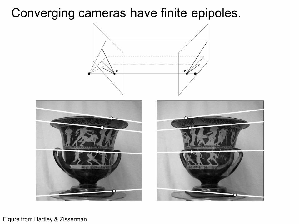
Converging cameras have finite epipoles.

Figure from Hartley & Zisserman

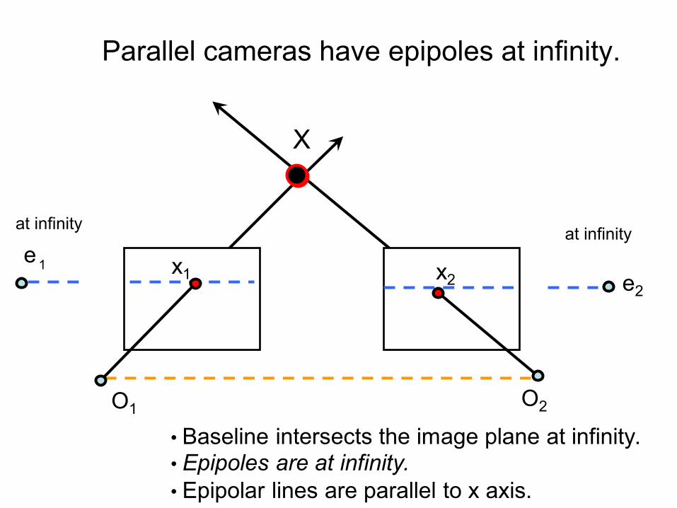
O1 O2

X

e2 x1 x2

e

Parallel cameras have epipoles at infinity.

• Baseline intersects the image plane at infinity. • Epipoles are at infinity. • Epipolar lines are parallel to x axis.

at infinityat infinity

1

Figure from Hartley & Zisserman

In parallel cameras search is only along x coord.

Slide credit: Kristen Grauman

is useful in stereo vision!

- Calibrated camera. Euclidean space.- We know the camera positions and camera matrices ==> E matrix - Given a point on left image, how can we find the corresponding point on right image?

Essential matrix: E

x E x = l'

Fundamental matrix: F

- Uncalibrated cameras. Projective space.- No additional information about the scene and camera is given ==> F matrix- Given a point on left image, how can I find the corresponding point on right image?

l’ = Fx x

In 2D a homography between In 3D a rotation and athe two images, changed with translation between the each pair of points. two coordinate systems.

x' l'= 0T

Fundamental matrix Fin the second image

Geometric derivation

A two-dimensional projective plane in the first image maps intoa pencil of epipolar lines in the second image.The scene plane not required for F. The connection between the fundamental matrix and transfer of points through a plane will bediscussed later.

The 3x3 matrix F has 7 degrees of freedom.

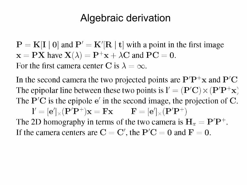
Algebraic derivation

other expressions

Properties

Coplanar point correspondes. 7 unknown. det(F) = 0.Given two projective cameras P, P', uniquely determines F.Cameras in 3D projective world frame! will see later the ambiguity

e' = P'C = P' [0 0 0 1] e = P' Pe' T [+]

finite cameras

Epipolar line homography

two DOF for e = 2 two DOF for e’ = 2three DOF for 1D homography mapping the pencil through eto pencil e' = 3. Seven DOF for F.

any point onthe baseline

k can be the line ewill not pass through point e e _1e_1 + e _2e_2 + 1 neq 0T T

Fundamental matrix for pure translation

two images !

motion not parallelwith the image plane

camera moves away

3D

2D

Properties of translational motion

×⎥⎥⎦

⎤

⎢⎢⎣

⎡=

0101-00000

F( )T1,0,0e'=

example:

y'y =⇔= 0Fxx'T

0]X|K[IPXx ==

⎥⎦⎤

⎢⎣⎡== Z

xKt]|K[IXP'x'-1

ZKt/xx' +=

ZX,Y,Z x/K)( -1T =

Motion starts at x and moves along the line x the e=e'=v. Faster if Z is smaller - e.g. the train. The epipolar line l'=Fx=[e]x x x [e]x x = 0x, x', v are collinear. Translation is auto-epipolar, but not valid in general.

4x1

useful in image rectification

t is in 3D

x =[X/Z Y/Z 1]T

X^T = [X Y Z 1]

along x axis

T

Motion: pure translation. Perpendicular to image plane.

move forward

• The epipoles have same position in both images. • Epipole is called FOE (focus of expansion) - camera toward; FOC (focus of contraction) - camera away

O'

e

e'

O

first

second

The general motion is different.

General motion

Zt/K'xRKK'x' -1 +=

[ ] 0Hxe''x =×T

[ ] 0x̂e''x =×T

P = K [I | 0] P' = K' [R | t]

homography followedby a translation of x

first term: rotation and internal parameterssecond term: depth only translation but not x

first rotation ==> H_inf = P'P+

^

imageposition only

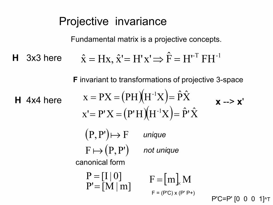
Projective invariance

-1-T FHH'F̂ x'H''x̂ Hx,x̂ =⇒==

Fundamental matrix is a projective concepts.

( )( ) X̂P̂XHPHPXx -1 ===

F invariant to transformations of projective 3-space

( )( ) X̂'P̂XHHP'XP'x' -1 ===

( ) FP'P,

( )P'P,Funique

not uniquecanonical form

m]|[MP'0]|[IP

== [ ] MmF ×=

H 3x3 here

F = (P'C) x (P' P+)P'C=P' [0 0 0 1]^T

H 4x4 here x --> x'

Projective ambiguity of cameras given FShow that if F is same for (P,P’) and (P,P’), there exists a projective transformation H so that P=PH P’=P’H

~ ~

~ ~

]a~|A~['P~ 0]|[IP~ a]|[AP' 0]|[IP ====

[ ] [ ] A~a~AaF ×× ==

( )T1 avAA~ kaa~ +== −klemma:

[ ] kaa~Fa~0AaaaF2rank

==== ⇒×

[ ] [ ] [ ] ( ) ( ) TavA-A~k0A-A~kaA~a~Aa =⇒=⇒= ×××

= −

−

kkIkH T1

1

v0

( ) 'P~]a|av-A[v0a]|[AHP' T1

T1

1==

= −

−

−

kkkkIk

22-15=7

can be for any k neq 0vector v in 3-dimension

4x4 matrix

|

PH = k^{-1} Ptwo camera - 15 DOF=fundamental matrix

T T T

3D projective~

first camera can be taken equal

fundamental matrix the samedecomposed two ways if

null space is a

e'^T e' neq 0line/point

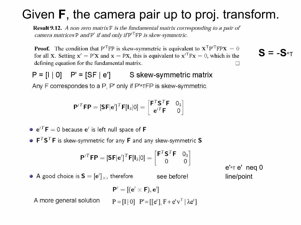
Given F, the camera pair up to proj. transform.

S = -S^T

0IKM

O O’

p p’

P

R, t

TRK'M K and K are known (calibrated cameras)

0I P TR P '

2''

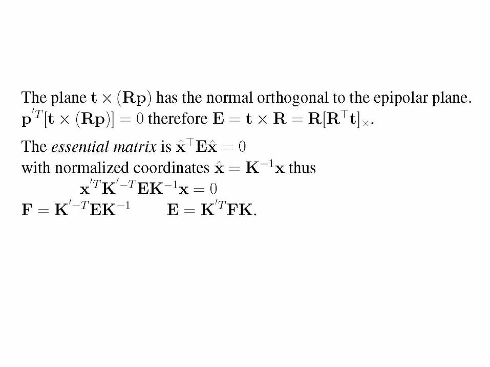
Essential Matrix

normalized camera matrix

k

Four possible reconstructions from E

only one solution where points is in front of both camerasone known point is enough

baseline reversed

the cameras rotatedby 180 degrees

Epipolar geometry: basic equation0Fxx'T =

separate known from unknown

0'''''' 333231232221131211 =++++++++ fyfxffyyfyxfyfxyfxxfx

[ ][ ] 0,,,,,,,,1,,,',',',',',' T333231232221131211 =fffffffffyxyyyxyxyxxx

data unknowns linear

0Af =

0f1''''''

1'''''' 111111111111=

⎥⎥

⎦

⎤

⎢⎢

⎣

⎡

nnnnnnnnnnnn yxyyyxyxyxxx

yxyyyxyxyxxxMMMMMMMMM

|| f || = 1

8-point algorithm

0

1´´´´´´

1´´´´´´1´´´´´´

33

32

31

23

22

21

13

12

11

222222222222

111111111111

=

⎥⎥⎥⎥⎥⎥⎥⎥⎥⎥⎥⎥

⎦

⎤

⎢⎢⎢⎢⎢⎢⎢⎢⎢⎢⎢⎢

⎣

⎡

⎥⎥⎥⎥

⎦

⎤

⎢⎢⎢⎢

⎣

⎡

fffffffff

yxyyyyxxxyxx

yxyyyyxxxyxxyxyyyyxxxyxx

nnnnnnnnnnnn

MMMMMMMMM

~10000 ~10000 ~10000 ~10000~100 ~100 1~100 ~100

! Orders of magnitude differenceBetween column of data matrix→ least-squares yields poor results

if is not normalized 8-point algorithm:

Like in Direct Linear Transformation (DLT)here we also have to normalize.

The singularity constraint

0Fe'T = 0Fe = 0detF= 2Frank =

T333

T222

T111

T

3

2

1VσUVσUVσUV

σσ

σUF ++=

⎥⎥

⎦

⎤

⎢⎢

⎣

⎡=

SVD from linearly computed F matrix (rank 3)

T222

T111

T2

1VσUVσUV

0σ

σUF' +=

⎥⎥

⎦

⎤

⎢⎢

⎣

⎡=

FF'-FminCompute closest rank-2 approximation

third singular value made zero

Minimum case – 7 point correspondences

0f1''''''

1''''''

777777777777

111111111111=

⎥⎥

⎦

⎤

⎢⎢

⎣

⎡

yxyyyxyxyxxx

yxyyyxyxyxxxMMMMMMMMM

( ) T9x9717x7 V0,0,σ,...,σdiagUA =

9x298 0]VA[V =⇒

1...70,)xλFF(x 21T =∀=+ iii

one parameter family of solutionsbut F1+λF2 not automatically rank 2

two dimensional null space

F1 F2

F

σ3

F7pts

(obtain 1 or 3 solutions)

0λλλ)λFFdet( 012

23

321 =+++=+ aaaa (cubic equation)

0)λIFFdet(Fdet)λFFdet( 1-12221 =+=+

.. impose rank 2

Compute possible λ as eigenvalues of

1-12 FF

One or three real solutions. Take the bestif there are three soution.

Parametrization of rank-2 F matrixExample: both epipolar as parameters, a total of 8 parameters.

4x(3x3)=36

Difficult to compute the fundamental matrix. A reparametrizationmeans maximizing the 9x8 Jacobian matrix dF/d(para) withthe used bases.

Hartley, 1995

In reality combined with RANSAC since there are outliers.

Linear Triangulation

linear triangulation not projective invariant

XP'x'=PXx =

0XPx =×

( ) ( )( ) ( )

( ) ( ) 0XpXp0XpXp0XpXp

1T2T

2T3T

1T3T

=−=−=−

yxyx

⎥⎥⎥

⎦

⎤

⎢⎢⎢

⎣

⎡

−−−−

=2T3T

1T3T

2T3T

1T3T

p'p''p'p''pppp

A

yxyx

homogeneous

1X =

)1,,,( ZYX

inhomogeneous

e)(HX)(AH-1 =

two per image point

DLT method:

4 equation but3 unknown

AH^{-1} X' same error because in

inhomogeneous method HX = X'[affine-invariant has 4th row (0 0 0 1)]

P and P' and x, x' givento find X in AX = 0

||X||=1 or X is not preserved: projective HX In the affine 4x4 transformation H has

Inhomogeneous is affine invariant, homogeneous is not.

not atinfinity

3 unknown

not used!

Triangulation in 3D

j=0,1, 2,...

d = R^{-1}K^{-1} x

T

Gold Standard method

Solved by Levenberg-Marquardt estimation. Needs the 3Dpoints X_i because the reprojection error is minimizes. Needs triangulation in 3D.

Some experiments:8-point -- solidgeometric error -- long dash algebraic error -- short dash iterative, but notgeometric error...

average 100 trials

symmetric epipolar Sampson distance

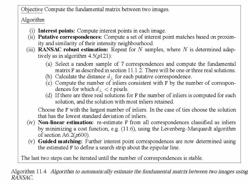
640x480 pixels (a), (b)~500 detected corners (c)(d)188 putative linked cornersshown on left image (e)89 outliers (f)99 inliers, consistent F (g)157 correspondences afterguided matching and LM (h)

Image pair rectificationsimplify stereo matching by warping the images

Apply projective transformation so that epipolar linescorrespond to horizontal scanlines

ee

map epipole e to (1,0,0)^T

try to minimize image distortion

problem when epipoles in (or close to) the images

Sec.11.12 in the booksomewhat different...

Planar rectification

Bring two views to standard stereo setup-- moves epipole to ∞ not possible when in/close to image

~ image size

(calibrated)

Distortion minimizationis part of it

(standard approach)

1 2

Image rectification. Loop and Zhang (1999).

The essential matrix is known. Denote E from image 1 to 2.

p' H' [i] H p = 0 -- 8 DOF each homography H, H' .

A homography is decomposed in

(shearing.similarity).projective -- order starts at right !

projective: epipolar lines become parallel in each image;

similarity: rotate the points into alignment with line maps

in the two images simultaneously. Its enough...

shearing: minimizing the horizontal distortion in each image.

T T

X

a b 00 1 00 0 1

two intervals: perpendicularknown aspect ratio => a, b

after projective and similarity

intervals given in original imgs

Rectification is useful.Slides of Loop, Zhang 1999.

Projective transformation.

Rotate, translate, uniformly scale only.

Shearing with u(u') parameters only, reduces the projectivedistortion separately in both images. e.g., to preserve perpendicularity and

aspect ratio of two line segments. The two cameras have some distortion.

before

afterFrom F, find the epipoles e, e'. The projective trans. by H' maps e' = (1 0 0)^T andthe projective transformation H by TLS sum[d(Hx_i, H'x'_i)]. Resample both images.

projective 2D transformationH' = GRTT translation takes a pointx_0 to the origin;R rotation e' to (f, 0, 1)^T;G from x point to infinity

pair of 512x512 images

affine transformationF has only 4DOF

zoom in: three pixelaverage y-disparity

0 0 a0 0 bc d e

Covariance of the estimated 3D point

Along z-axis is much larger covariance than along x- or y-axis.

IMPLICIT FUNCTION COVARIANCE

Theexplicit case we have already seen. Ify = φ(x) the covarianceof the output in first order approximation,Σy is

Σy =∂φ(x)

∂xΣx

(

∂φ(x)

∂x

)⊤

where the Jacobian is computed close to the averagex.

The case of theimplicit function covariance is more complicated.The criterion functionC(x, z) takes the values of the measurementvectorsx ∈ Rm and the output valuesz ∈ Rp and returns a scalarwhich in ideal conditions has value 0, that isRm × Rp → R. Weneed at leastp equations so the implicit system of equation is

Φ =

(

∂C

∂z

)⊤

whereΦ is a (p, 1) vector. Letx0 the measurement vector whichgivesy0 a local minimum ofC(x, z). If the HessianH of C(x, z)

with respect toz invertible around(x0,y0), then the two relations ”yis a local minimum ofC(x, z) with respect toz” and y = φ(x) areequivalent.

The vectorΦ containsi = 1, . . . , p equations

ψi(x,φ(x)) = 0 .

The total derivative ofψi in xj, wherej is one of1, . . . , m, is

∂ψi

∂xj

+

p∑

k=1

∂ψi

∂φk(x)

∂φk(x)

∂xj

= 0

andφk(x) is the notation forzk. Moving∂ψi

∂xj

to the right side and

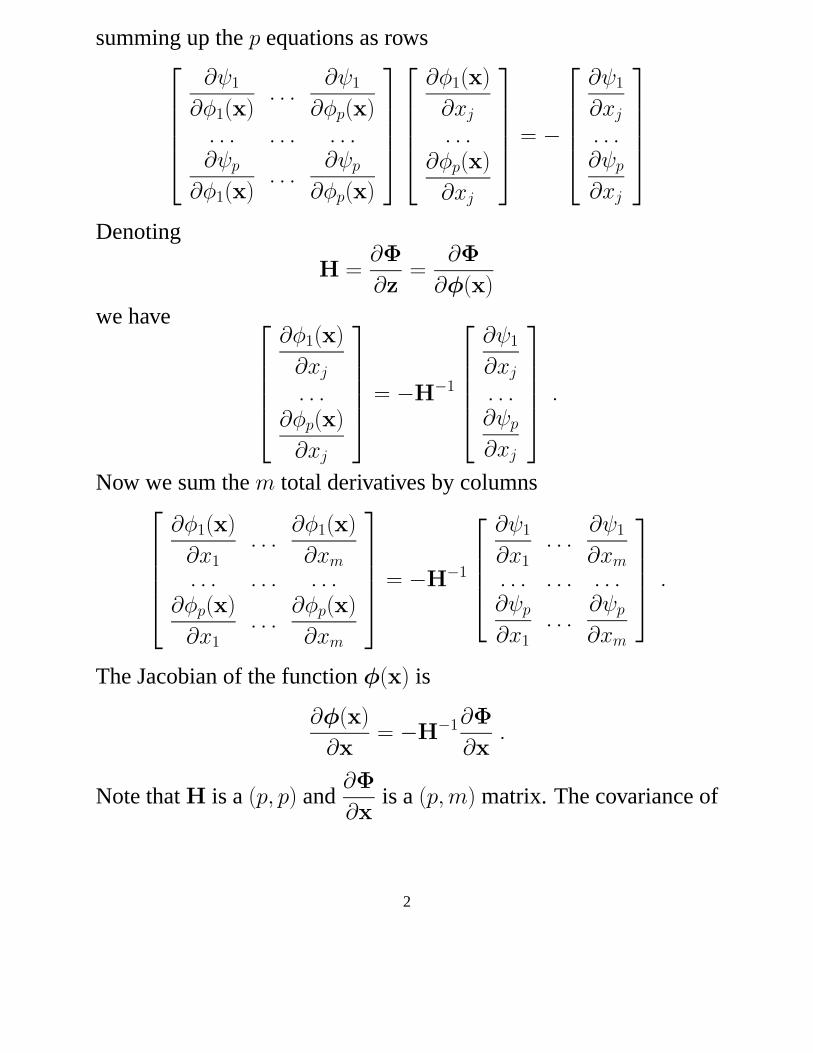
summing up thep equations as rows

∂ψ1

∂φ1(x). . .

∂ψ1

∂φp(x). . . . . . . . .∂ψp

∂φ1(x). . .

∂ψp

∂φp(x)

∂φ1(x)

∂xj

. . .∂φp(x)

∂xj

= −

∂ψ1

∂xj

. . .∂ψp

∂xj

Denoting

H =∂Φ

∂z=

∂Φ

∂φ(x)

we have

∂φ1(x)

∂xj

. . .∂φp(x)

∂xj

= −H−1

∂ψ1

∂xj

. . .∂ψp

∂xj

.

Now we sum them total derivatives by columns

∂φ1(x)

∂x1

. . .∂φ1(x)

∂xm

. . . . . . . . .∂φp(x)

∂x1

. . .∂φp(x)

∂xm

= −H−1

∂ψ1

∂x1

. . .∂ψ1

∂xm

. . . . . . . . .∂ψp

∂x1

. . .∂ψp

∂xm

.

The Jacobian of the functionφ(x) is

∂φ(x)

∂x= −H−1

∂Φ

∂x.

Note thatH is a(p, p) and∂Φ

∂xis a(p, m) matrix. The covariance of

2

the output therefore becomes a(p, p) matrix

Σz =

(

∂Φ

∂z

)−1∂Φ

∂xΣx

(

∂Φ

∂x

)⊤ (

∂Φ

∂z

)−⊤

= H−1∂Φ

∂xΣx

(

∂Φ

∂x

)⊤

H−⊤ .

Sum of squares implicit function.The criterion function becomes

C(x, z) =

n∑

i=1

C2

i (xi, z)

wherex = [x⊤1 , . . . ,x⊤

n ]⊤ and the implicit equation is

Φ = 2

n∑

i=1

Ci

(

∂Ci

∂z

)⊤

.

Neglecting the second order derivative of the Hessian inH and com-

puting∂Φ

∂xresults

H ≈ 2

n∑

i=1

(

∂Ci

∂z

)⊤∂Ci

∂z

∂Φ

∂x≈ 2

n∑

i=1

(

∂Ci

∂z

)⊤∂Ci

∂x.

The noise of the input is independent and therefore

Σx = diag(Σx1, . . . , Σxn

) .

The covariance of the output becomes

Σz = 4 H−1

n∑

i=1

(

∂Ci

∂z

)⊤∂Ci

∂xi

Σxi

(

∂Ci

∂xi

)⊤∂Ci

∂zH−⊤ .

3

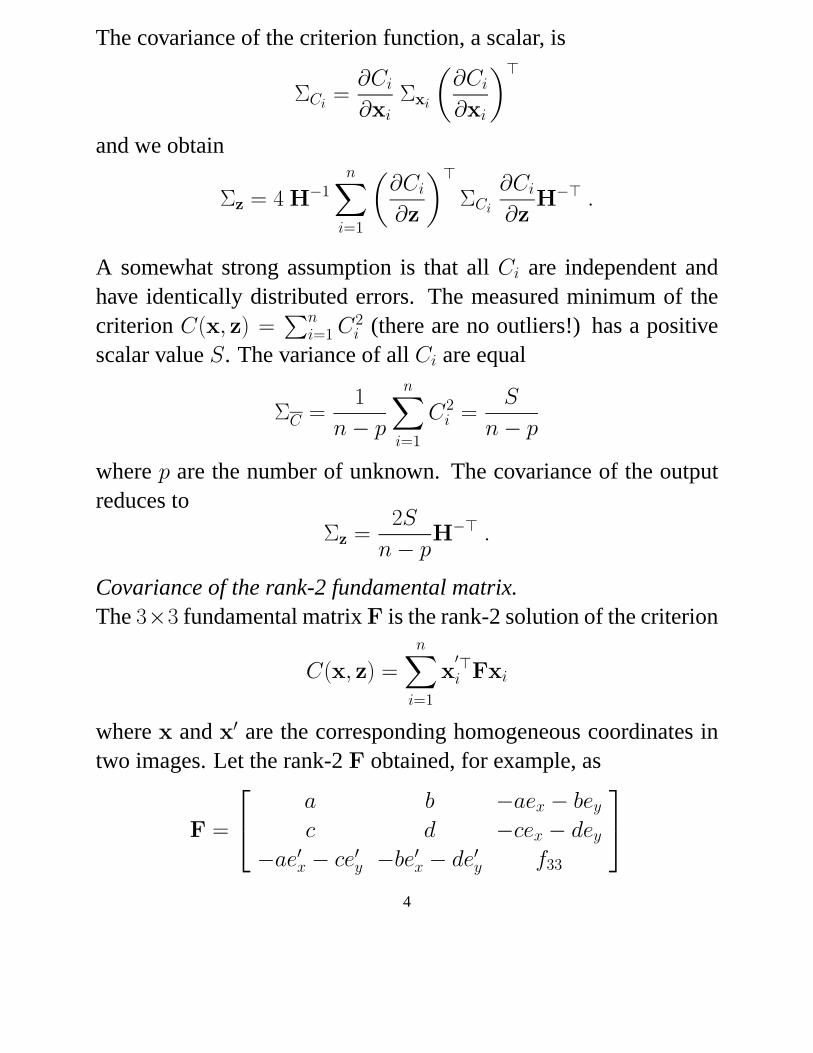
The covariance of the criterion function, a scalar, is

ΣCi=

∂Ci

∂xi

Σxi

(

∂Ci

∂xi

)⊤

and we obtain

Σz = 4 H−1

n∑

i=1

(

∂Ci

∂z

)⊤

ΣCi

∂Ci

∂zH−⊤ .

A somewhat strong assumption is that allCi are independent andhave identically distributed errors. The measured minimum of thecriterionC(x, z) =

∑ni=1

C2i (there are no outliers!) has a positive

scalar valueS. The variance of allCi are equal

ΣC =1

n − p

n∑

i=1

C2

i =S

n − p

wherep are the number of unknown. The covariance of the outputreduces to

Σz =2S

n − pH−⊤ .

Covariance of the rank-2 fundamental matrix.The3×3 fundamental matrixF is the rank-2 solution of the criterion

C(x, z) =

n∑

i=1

x′⊤i Fxi

wherex andx′ are the corresponding homogeneous coordinates intwo images. Let the rank-2F obtained, for example, as

F =

a b −aex − bey

c d −cex − dey

−ae′x − ce′y −be′x − de′y f33

4

whereex, ey and e′x, e′y are the inhomogeneous coordinates of the

epipoles in the two images, and

f33 = (aex + bey)e′x + (cex + dey)e

′y .

There are seven unknowns since you divide with a scale factor. Thevectorf is obtained from the matrixF, which is rank seven.

The criterion function isC(x, f7), wherex = [x⊤1 ,x

′⊤1 , . . . ,x⊤

n ,x′⊤n ]⊤.

The covariance off , obtained in the simplest case, is

Σf7 =2S

n − pH−⊤

and H is the approximative Hessian inf7, the z, computed fromC(x, f7). The final covariance is a9 × 9 matrix of rank seven

ΣF =∂F(f7)

∂f7Σf7

∂F(f7)

∂f7

⊤

and each∂Fi,j

∂f7, i, j = 1, 2, 3 is a (1, p) vector. Each variance is

computed separately. The last two singular values ofΣF have to bezero.

5