Math Geosci (2012) 44:309–326DOI 10.1007/s11004-011-9380-3

Earthquake Modelling at the Country Level UsingAggregated Spatio-Temporal Point Processes

M.N.M. van Lieshout · A. Stein

Received: 28 March 2011 / Accepted: 7 December 2011 / Published online: 17 January 2012© The Author(s) 2011. This article is published with open access at Springerlink.com

Abstract The goal of this paper is to derive a hazard map for earthquake occurrencesin Pakistan from a catalogue that contains spatial coordinates of shallow earthquakesof magnitude 4.5 or larger aggregated over calendar years. We test relative temporalstationarity by the KPSS statistic and use the inhomogeneous J -function to test forinter-point interactions. We then formulate a cluster model, and de-convolve in orderto calculate the hazard map, and verify that no particular year has an undue influenceon the map. Within the borders of the single country, the KPSS test did not show anydeviation from homogeneity in the spatial intensities. The inhomogeneous J -functionindicated clustering that could not be attributed to inhomogeneity, and the analysis ofaftershocks showed some evidence of two major shocks instead of one during the2005 Kashmir earthquake disaster. Thus, the spatial point pattern analysis carried outfor these data was insightful in various aspects and the hazard map that was obtainedmay lead to improved measures to protect the population against the disastrous effectsof earthquakes.

Keywords Aftershocks · Cluster point process · De-convolution · Hazard map ·Inhomogeneous J -function · Intensity function · Relative stationarity test

In memory of Julian E. Besag.

M.N.M. van LieshoutProbability, Networks and Algorithms, CWI, Amsterdam, The Netherlands

A. Stein (�)Faculty of Geo-Information Science and Earth Observation (ITC), University of Twente, Enschede,The Netherlandse-mail: stein@itc.nl

310 Math Geosci (2012) 44:309–326

1 Introduction

Disasters such as earthquakes occur at apparently erratic seismic locations and atunexpected moments. Processes generating earthquakes are prominent in earthquakeprone areas that are at least partly determined by geological faults and occur, in par-ticular, close to subduction zones. An earthquake describes both a sudden slip on afault and the resulting ground shaking and radiated seismic energy caused by the slip,by volcanic or magmatic activity, or other sudden stress changes in the earth. Therelease of energy at an unanticipated moment may then appear at the earth surfaceand is registered as the main shock. Main shocks are usually followed by aftershocksthat are smaller than the main shock and within 1–2 rupture lengths distance from themain shock. Aftershocks can continue over a period of weeks, months, or years. Ingeneral, the larger the main shock, the larger and more numerous the aftershocks, andthe longer they will continue. Other types of clusters known as swarms also occur.Such clusters are more diffuse and can be distinguished from aftershock sequencesby their showing no clear correlation with a main shock, nor the typical decay infrequency and magnitude common to aftershock patterns.

In the analysis of earthquakes, spatio-temporal Hawkes processes, in particu-lar, Ogata’s Epidemic Type Aftershock-Sequences (ETAS) model, have become thestandard first approximation for seismic catalogue data that come in the form ofa list of earthquake locations, their times, and magnitudes (Ogata 1988). An ex-cellent review is given by Ogata (1998) who also gives historical references. Insuch a Hawkes process, immigrants arrive according to a temporal Poisson pro-cess and are marked by their spatial location and other attributes as required. Eachimmigrant generates a finite marked Poisson process of ‘offspring’ with an inten-sity function that depends on the parent, independently of other immigrants. Theoffspring in their turn also generate offspring independently of all others, and soon. In other words, each immigrant produces a branching process of descendants.Therefore, a Hawkes process can also be described as a marked Poisson cluster pro-cess. An alternative to Hawkes processes is to use a Neymann–Scott process whichrestricts the branching to only one generation of descendants (Vere-Jones 1970;Adamopoulos 1976).

In the earthquake context, the offspring are swarms or aftershock clusters; theirnumber typically depends on the magnitude of the parent, their temporal displace-ment follows the Omori (Pareto) power law. With regard to the marks, the magni-tudes are widely assumed to follow a shifted exponential distribution; for the spatialdisplacements, various probability distributions have been tried. Examples, includingthe spherical Gaussian distribution we shall use in Sect. 6, are given in Ogata (1998),Holden et al. (2003), Daley and Vere-Jones (2003, 2008). See also Vere-Jones (1970),Vere-Jones and Musmeci (1992), Shurygin (1993), or Zhuang et al. (2002).

The advantage of focusing on the temporal dimension and treating other variablesof interest (magnitude and spatial location) as marks is that a conditional intensitycan be written down. Consequently, a likelihood function is available in closed formand can be used for inference. For details, see Ogata (1998). Moreover, many of theabove papers consider the island states of Japan and New Zealand for which edgeeffects seem not to be an issue.

Math Geosci (2012) 44:309–326 311

Early work in the earthquake literature includes a study into the clustering of earth-quakes (Adamopoulos 1976) and the use of a Poisson process for the long-term pre-diction of seismicity for linear zones (Shurygin 1993). More recent contributions havebeen made by Holden et al. (2003) who developed a marked point process model forearthquakes, focusing on parameter estimation, by Lucio and Castelucio de Brito(2004), who use simulations to detect randomness in spatial point patterns with anapplication to seismology, by Pei et al. (2007) who studied vulnerability to earth-quakes and aftershocks in a Bayesian framework, and by Pei (2011) who developed anon-parametric index for the numbers of events in an earthquake cluster on the basisof the nearest neighbour distance with an application to the earthquake catalogue ofChina. Our paper adds to the current literature in that non-homogeneity is taken intoaccount explicitly both in the testing and in the spatial modelling.

The aim of this study is to explore spatial statistical techniques for data aggregatedover time for which an explicit likelihood function is not available. Attention focuseson Pakistan, for which country annual patterns of earthquakes have been recorded formore than 35 years. During this period, two major earthquakes of magnitude largerthan seven were recorded: one occurring in 1997 and the major Kashmir earthquakeof 2005. Moreover, seismic activity in neighbouring countries may well influenceoccurrences inside Pakistan.

The plan of this paper is as follows. In Sect. 2 we discuss the data. In Sect. 3,we pool all normal years and calculate a kernel estimator for the pooled intensitymap of earthquake occurrence. This map is then used to test for relative temporalstationarity (Sect. 4) and inter-point interactions (Sect. 5). We conclude that there isno evidence for a temporal trend, but that there does appear to be clustering in thedata that cannot be attributed to geological inhomogeneity. These observations leadus to look at the patterns of aftershocks in the major earthquake years 1997 and 2005in Sect. 6 in order to formulate a cluster model (Sect. 7), from which a hazard mapcan be derived. Such a map provides information about the likelihood of earthquakeoccurrences in an area of interest, but does not predict when the next disaster willstrike. We verify in Sect. 8 that the hazard map is not dominated by exceptional yearsusing the leave-one-out principle. The paper closes with a critical discussion andsummary of the main findings.

2 Background and Data

Pakistan is a country that is regularly affected by earthquakes. The reason for thevulnerability of the country to earthquakes is the subduction of the Indo-Australiancontinental plate under the Eurasian plate with its two associated convergence zones.One such zone crosses the country from approximately its south-western border withthe Arabic Sea to Kashmir in the North East. The other convergence zone crosses thenorthern part of the country in the east-west direction and is the direct cause of theHimalayan orogeny. Pakistan-administered Kashmir lies in the area where the twozones meet. The geological activity born out of the collisions is the cause of unstableseismicity in the region.

Earthquakes can be severe with a devastating effect on human life and property.Two major earthquakes were recorded in 1997 and 2005 with magnitudes of 7.3 and

312 Math Geosci (2012) 44:309–326

7.6, respectively. The 1997 earthquake occurred along the convergence zone runningfrom the South West to the North East and resulted in about seventy casualties. The2005 Kashmir earthquake, however, was catastrophic with at least 86,000 casualties.The Pakistan Meteorological Department estimated a 5.2 magnitude on the Richterscale, whereas the United States Geological Survey (USGS) measured its magnitudeas at least 7.6 on the moment magnitude scale, classifying the quake as major. Itsepicentre lay about 19 km north-east of the city of Muzaffarabad, its hypocenter waslocated at a depth of 26 km below the surface.

Such big earthquakes are accompanied by many aftershocks. For example in 2005,the city of Karachi (more than 1,000 km away from the epicentre) experienced aminor aftershock. There were many secondary earthquakes in the region, mainly tothe north-west of the epicentre. A total of 147 aftershocks were registered in the firstday after the initial quake. On October 19, a series of strong aftershocks occurredabout 65 km north-northwest of Muzaffarabad. As an aside, note that aftershocks caneven be stronger than the main earthquake itself.

In addition to such major shocks, that are still relatively rare, many smaller shockshave been recorded (see http://earthquake.usgs.gov/earthquakes for a list of earth-quakes since 1973). The majority of tectonic earthquakes originate at depths not ex-ceeding tens of kilometres. Those occurring at a depth of less than 70 km are clas-sified as shallow. Earthquakes that originate below this upper crust are classified asintermediate or deep. See Molnar and Chen (1982) for further details. Clearly, theimpact of an earthquake depends on its epicentre, its depth as well as its magnitude.Minor earthquakes occur very frequently and may not even be noticed or recorded.Therefore, we focus on those having a magnitude of at least 4.5 for which records arebelieved to be exhaustive (Van der Meijde, pers. comm.).

To summarize, our data (available from the authors on request) consist of the an-nual patterns of shallow earthquakes of magnitude 4.5 or higher in Pakistan duringthe period 1973–2008. The country level is appropriate, as most political and riskmanagement actions are taken at this level. However, to avoid edge effects, we mustsometimes refer to data on earthquakes across the border. For each event, its locationand magnitude is recorded. For the major earthquake years 1997 and 2005, also thetimes at which shocks occurred in the month following the main one are available.

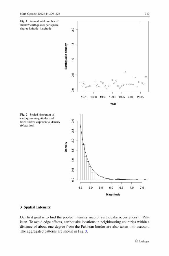
In Fig. 1, we plot the annual number of such earthquakes per square degreelatitude-longitude (y-axis) over the period 1973–2008 (x-axis). Note that the clearlyvisible outlier corresponds to the Kashmir earthquake in 2005 that generated a largenumber of aftershocks. The number of aftershocks in 1997 was considerably less andtheir pattern more diffuse.

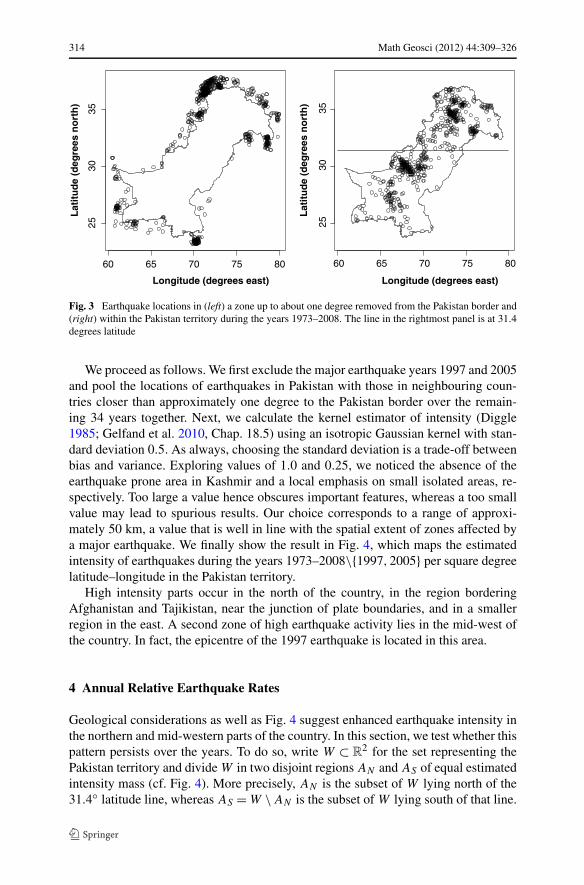
A scaled histogram of the observed magnitudes is presented in Fig. 2. In accor-dance with the Gutenberg–Richter power law, we fit a shifted exponential probabilitydensity βe−β(m−4.5) for m ≥ 4.5 and 0 elsewhere. The rate parameter β can be inter-preted as follows: 1/β is the expected excess magnitude with respect to the thresholdvalue 4.5. For our data, the mean excess is 0.354 so the unknown parameter can beestimated by β = 2.28. Comparing the graph of the fitted shifted exponential proba-bility density to the histogram indicates an adequate fit (Fig. 2).

Math Geosci (2012) 44:309–326 313

Fig. 1 Annual total number ofshallow earthquakes per squaredegree latitude–longitude

Fig. 2 Scaled histogram ofearthquake magnitudes andfitted shifted exponential density(black line)

3 Spatial Intensity

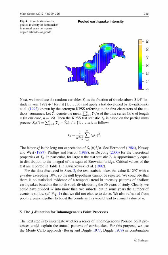
Our first goal is to find the pooled intensity map of earthquake occurrences in Pak-istan. To avoid edge effects, earthquake locations in neighbouring countries within adistance of about one degree from the Pakistan border are also taken into account.The aggregated patterns are shown in Fig. 3.

314 Math Geosci (2012) 44:309–326

Fig. 3 Earthquake locations in (left) a zone up to about one degree removed from the Pakistan border and(right) within the Pakistan territory during the years 1973–2008. The line in the rightmost panel is at 31.4degrees latitude

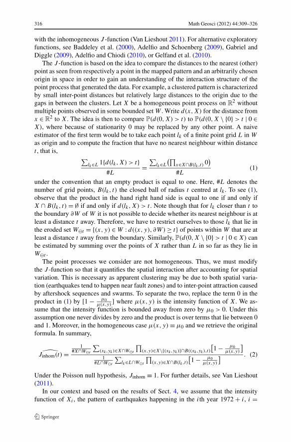
We proceed as follows. We first exclude the major earthquake years 1997 and 2005and pool the locations of earthquakes in Pakistan with those in neighbouring coun-tries closer than approximately one degree to the Pakistan border over the remain-ing 34 years together. Next, we calculate the kernel estimator of intensity (Diggle1985; Gelfand et al. 2010, Chap. 18.5) using an isotropic Gaussian kernel with stan-dard deviation 0.5. As always, choosing the standard deviation is a trade-off betweenbias and variance. Exploring values of 1.0 and 0.25, we noticed the absence of theearthquake prone area in Kashmir and a local emphasis on small isolated areas, re-spectively. Too large a value hence obscures important features, whereas a too smallvalue may lead to spurious results. Our choice corresponds to a range of approxi-mately 50 km, a value that is well in line with the spatial extent of zones affected bya major earthquake. We finally show the result in Fig. 4, which maps the estimatedintensity of earthquakes during the years 1973–2008\{1997,2005} per square degreelatitude–longitude in the Pakistan territory.

High intensity parts occur in the north of the country, in the region borderingAfghanistan and Tajikistan, near the junction of plate boundaries, and in a smallerregion in the east. A second zone of high earthquake activity lies in the mid-west ofthe country. In fact, the epicentre of the 1997 earthquake is located in this area.

4 Annual Relative Earthquake Rates

Geological considerations as well as Fig. 4 suggest enhanced earthquake intensity inthe northern and mid-western parts of the country. In this section, we test whether thispattern persists over the years. To do so, write W ⊂ R

2 for the set representing thePakistan territory and divide W in two disjoint regions AN and AS of equal estimatedintensity mass (cf. Fig. 4). More precisely, AN is the subset of W lying north of the31.4◦ latitude line, whereas AS = W \ AN is the subset of W lying south of that line.

Math Geosci (2012) 44:309–326 315

Fig. 4 Kernel estimator forpooled intensity of earthquakesin normal years per squaredegree latitude–longitude

Next, we introduce the random variables Yi as the fraction of shocks above 31.4◦ lat-itude in year 1972 + i for i ∈ {1, . . . ,36} and apply a test developed by Kwiatkowskiet al. (1992) known by the acronym KPSS referring to the first characters of the au-thors’ surnames. Let Yn denote the mean

∑ni=1 Yi/n of the time series (Yi)i of length

n (in our case, n = 36). Then the KPSS test statistic Tn is based on the partial sumsprocess Sn(i) = ∑i

j=1(Yj − Yn), i ∈ {1, . . . , n}, as follows

Tn = 1

n2s2n

n∑

i=1

Sn(i)2.

The factor s2n is the long run expectation of Sn(n)2/n. See Herrndorf (1984), Newey

and West (1987), Phillips and Perron (1988), or De Jong (2000) for the theoreticalproperties of Tn. In particular, for large n the test statistic Tn is approximately equalin distribution to the integral of the squared Brownian bridge. Critical values of thetest are reported in Table 1 in Kwiatkowski et al. (1992).

For the data discussed in Sect. 2, the test statistic takes the value 0.1297 with ap-value exceeding 10%, so the null hypothesis cannot be rejected. We conclude thatthere is no statistical evidence of a temporal trend in intensity patterns of shallowearthquakes based on the north-south divide during the 36 years of study. Clearly, wecould have divided W into more than two subsets, but in some years the number ofevents is so low (cf. Fig. 1) that we did not choose to do so. We also refrained frompooling years together to boost the counts as this would lead to a small value of n.

5 The J -Function for Inhomogeneous Point Processes

The next step is to investigate whether a series of inhomogeneous Poisson point pro-cesses could explain the annual patterns of earthquakes. For this purpose, we usethe Monte Carlo approach (Besag and Diggle 1977; Diggle 1979) in combination

316 Math Geosci (2012) 44:309–326

with the inhomogeneous J -function (Van Lieshout 2011). For alternative exploratoryfunctions, see Baddeley et al. (2000), Adelfio and Schoenberg (2009), Gabriel andDiggle (2009), Adelfio and Chiodi (2010), or Gelfand et al. (2010).

The J -function is based on the idea to compare the distances to the nearest (other)point as seen from respectively a point in the mapped pattern and an arbitrarily chosenorigin in space in order to gain an understanding of the interaction structure of thepoint process that generated the data. For example, a clustered pattern is characterizedby small inter-point distances but relatively large distances to the origin due to thegaps in between the clusters. Let X be a homogeneous point process on R

2 withoutmultiple points observed in some bounded set W . Write d(x,X) for the distance fromx ∈ R

2 to X. The idea is then to compare P(d(0,X) > t) to P(d(0,X \ {0} > t | 0 ∈X), where because of stationarity 0 may be replaced by any other point. A naiveestimator of the first term would be to take each point lk of a finite point grid L in W

as origin and to compute the fraction that have no nearest neighbour within distancet , that is,

∑lk∈L 1{d(lk,X) > t}

#L=

∑lk∈L

(∏x∈X∩B(lk,t)

0)

#L(1)

under the convention that an empty product is equal to one. Here, #L denotes thenumber of grid points, B(lk, t) the closed ball of radius t centred at lk . To see (1),observe that the product in the hand right hand side is equal to one if and only ifX ∩ B(lk, t) = ∅ if and only if d(lk,X) > t . Note though that for lk closer than t tothe boundary ∂W of W it is not possible to decide whether its nearest neighbour is atleast a distance t away. Therefore, we have to restrict ourselves to those lk that lie inthe eroded set W�t = {(x, y) ∈ W : d((x, y), ∂W) ≥ t} of points within W that are atleast a distance t away from the boundary. Similarly, P(d(0,X \ {0} > t | 0 ∈ X) canbe estimated by summing over the points of X rather than L in so far as they lie inW�t .

The point processes we consider are not homogeneous. Thus, we must modifythe J -function so that it quantifies the spatial interaction after accounting for spatialvariation. This is necessary as apparent clustering may be due to both spatial varia-tion (earthquakes tend to happen near fault zones) and to inter-point attraction causedby aftershock sequences and swarms. To separate the two, replace the term 0 in theproduct in (1) by [1 − μ0

μ(x,y)] where μ(x, y) is the intensity function of X. We as-

sume that the intensity function is bounded away from zero by μ0 > 0. Under thisassumption one never divides by zero and the product is over terms that lie between 0and 1. Moreover, in the homogeneous case μ(x, y) ≡ μ0 and we retrieve the originalformula. In summary,

Jinhom(t) =1

#X∩W�t

∑(xk,yk)∈X∩W�t

∏(x,y)∈X\{(xk,yk)}∩B((xk,yk),t)

[1 − μ0

μ(x,y)

]

1#L∩W�t

∑lk∈L∩W�t

∏(x,y)∈X∩B(lk,t)

[1 − μ0

μ(x,y)

] . (2)

Under the Poisson null hypothesis, Jinhom ≡ 1. For further details, see Van Lieshout(2011).

In our context and based on the results of Sect. 4, we assume that the intensityfunction of Xi , the pattern of earthquakes happening in the ith year 1972 + i, i =

Math Geosci (2012) 44:309–326 317

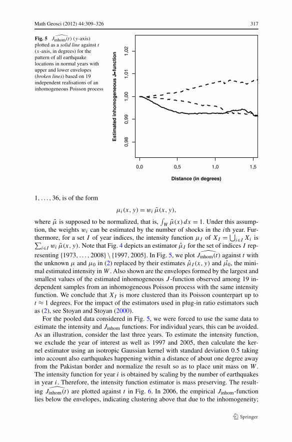
Fig. 5 Jinhom(t) (y-axis)plotted as a solid line against t

(x-axis, in degrees) for thepattern of all earthquakelocations in normal years withupper and lower envelopes(broken lines) based on 19independent realisations of aninhomogeneous Poisson process

1, . . . ,36, is of the form

μi(x, y) = wi μ(x, y),

where μ is supposed to be normalized, that is,∫W

μ(x) dx = 1. Under this assump-tion, the weights wi can be estimated by the number of shocks in the ith year. Fur-thermore, for a set I of year indices, the intensity function μI of XI = ⋃

i∈I Xi is∑i∈I wi μ(x, y). Note that Fig. 4 depicts an estimator μI for the set of indices I rep-

resenting {1973, . . . ,2008} \ {1997,2005}. In Fig. 5, we plot Jinhom(t) against t withthe unknown μ and μ0 in (2) replaced by their estimates μI (x, y) and μ0, the mini-mal estimated intensity in W . Also shown are the envelopes formed by the largest andsmallest values of the estimated inhomogeneous J -function observed among 19 in-dependent samples from an inhomogeneous Poisson process with the same intensityfunction. We conclude that XI is more clustered than its Poisson counterpart up tot ≈ 1 degrees. For the impact of the estimators used in plug-in ratio estimators suchas (2), see Stoyan and Stoyan (2000).

For the pooled data considered in Fig. 5, we were forced to use the same data toestimate the intensity and Jinhom functions. For individual years, this can be avoided.As an illustration, consider the last three years. To estimate the intensity function,we exclude the year of interest as well as 1997 and 2005, then calculate the ker-nel estimator using an isotropic Gaussian kernel with standard deviation 0.5 takinginto account also earthquakes happening within a distance of about one degree awayfrom the Pakistan border and normalize the result so as to place unit mass on W .The intensity function for year i is obtained by scaling by the number of earthquakesin year i. Therefore, the intensity function estimator is mass preserving. The result-ing Jinhom(t) are plotted against t in Fig. 6. In 2006, the empirical Jinhom-functionlies below the envelopes, indicating clustering above that due to the inhomogeneity;

318 Math Geosci (2012) 44:309–326

Fig. 6 Jinhom(t) (y-axis) plotted as solid lines against t (x-axis, in degrees) for the patterns of earthquakesin 2006 (leftmost frame), 2007 (middle frame) and 2008 (rightmost frame) with upper and lower envelopes(broken lines) based on 19 independent realisations of an inhomogeneous Poisson process

the pattern in 2008 also exhibits strong attraction between the points, especially forsmall t . In 2007, there is significant but milder clustering at intermediate range.

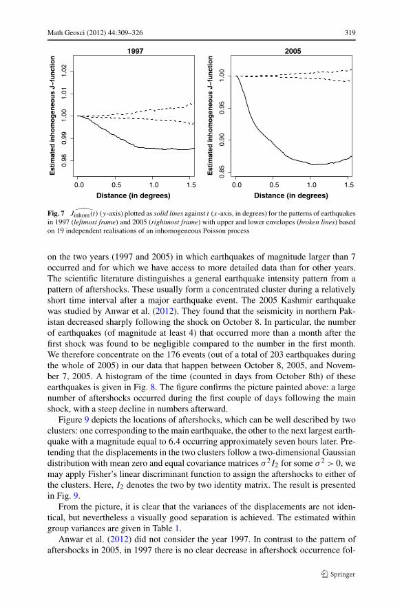
For the years in which an earthquake of magnitude of at least seven occurred, thatis, for 1997 and 2005, the estimated inhomogeneous J -function strongly suggestsclustering after accounting for the effect of spatial variability, cf. Fig. 7.

6 Aftershocks in the Major Earthquake Years

From the two previous sections, we conclude that there is no evidence for a temporaltrend, but that there appears to be clustering in the data that cannot be attributed to ge-ological inhomogeneity. In order to be able to formulate a cluster model, informationabout the spread of aftershocks around a main event is needed. We therefore focus

Math Geosci (2012) 44:309–326 319

Fig. 7 Jinhom(t) (y-axis) plotted as solid lines against t (x-axis, in degrees) for the patterns of earthquakesin 1997 (leftmost frame) and 2005 (rightmost frame) with upper and lower envelopes (broken lines) basedon 19 independent realisations of an inhomogeneous Poisson process

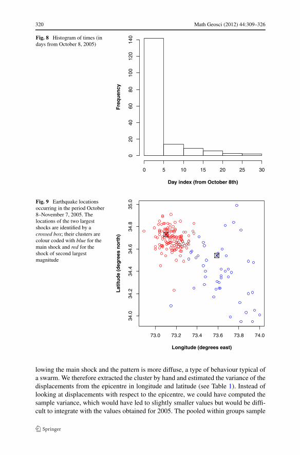
on the two years (1997 and 2005) in which earthquakes of magnitude larger than 7occurred and for which we have access to more detailed data than for other years.The scientific literature distinguishes a general earthquake intensity pattern from apattern of aftershocks. These usually form a concentrated cluster during a relativelyshort time interval after a major earthquake event. The 2005 Kashmir earthquakewas studied by Anwar et al. (2012). They found that the seismicity in northern Pak-istan decreased sharply following the shock on October 8. In particular, the numberof earthquakes (of magnitude at least 4) that occurred more than a month after thefirst shock was found to be negligible compared to the number in the first month.We therefore concentrate on the 176 events (out of a total of 203 earthquakes duringthe whole of 2005) in our data that happen between October 8, 2005, and Novem-ber 7, 2005. A histogram of the time (counted in days from October 8th) of theseearthquakes is given in Fig. 8. The figure confirms the picture painted above: a largenumber of aftershocks occurred during the first couple of days following the mainshock, with a steep decline in numbers afterward.

Figure 9 depicts the locations of aftershocks, which can be well described by twoclusters: one corresponding to the main earthquake, the other to the next largest earth-quake with a magnitude equal to 6.4 occurring approximately seven hours later. Pre-tending that the displacements in the two clusters follow a two-dimensional Gaussiandistribution with mean zero and equal covariance matrices σ 2I2 for some σ 2 > 0, wemay apply Fisher’s linear discriminant function to assign the aftershocks to either ofthe clusters. Here, I2 denotes the two by two identity matrix. The result is presentedin Fig. 9.

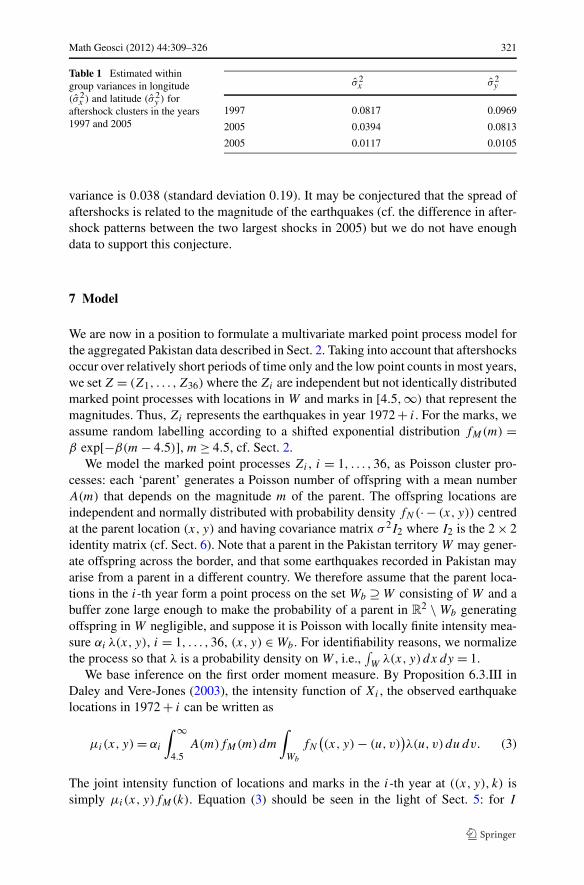
From the picture, it is clear that the variances of the displacements are not iden-tical, but nevertheless a visually good separation is achieved. The estimated withingroup variances are given in Table 1.

Anwar et al. (2012) did not consider the year 1997. In contrast to the pattern ofaftershocks in 2005, in 1997 there is no clear decrease in aftershock occurrence fol-

320 Math Geosci (2012) 44:309–326

Fig. 8 Histogram of times (indays from October 8, 2005)

Fig. 9 Earthquake locationsoccurring in the period October8–November 7, 2005. Thelocations of the two largestshocks are identified by acrossed box; their clusters arecolour coded with blue for themain shock and red for theshock of second largestmagnitude

lowing the main shock and the pattern is more diffuse, a type of behaviour typical ofa swarm. We therefore extracted the cluster by hand and estimated the variance of thedisplacements from the epicentre in longitude and latitude (see Table 1). Instead oflooking at displacements with respect to the epicentre, we could have computed thesample variance, which would have led to slightly smaller values but would be diffi-cult to integrate with the values obtained for 2005. The pooled within groups sample

Math Geosci (2012) 44:309–326 321

Table 1 Estimated withingroup variances in longitude(σ 2

x ) and latitude (σ 2y ) for

aftershock clusters in the years1997 and 2005

σ 2x σ 2

y

1997 0.0817 0.0969

2005 0.0394 0.0813

2005 0.0117 0.0105

variance is 0.038 (standard deviation 0.19). It may be conjectured that the spread ofaftershocks is related to the magnitude of the earthquakes (cf. the difference in after-shock patterns between the two largest shocks in 2005) but we do not have enoughdata to support this conjecture.

7 Model

We are now in a position to formulate a multivariate marked point process model forthe aggregated Pakistan data described in Sect. 2. Taking into account that aftershocksoccur over relatively short periods of time only and the low point counts in most years,we set Z = (Z1, . . . ,Z36) where the Zi are independent but not identically distributedmarked point processes with locations in W and marks in [4.5,∞) that represent themagnitudes. Thus, Zi represents the earthquakes in year 1972 + i. For the marks, weassume random labelling according to a shifted exponential distribution fM(m) =β exp[−β(m − 4.5)], m ≥ 4.5, cf. Sect. 2.

We model the marked point processes Zi , i = 1, . . . ,36, as Poisson cluster pro-cesses: each ‘parent’ generates a Poisson number of offspring with a mean numberA(m) that depends on the magnitude m of the parent. The offspring locations areindependent and normally distributed with probability density fN(· − (x, y)) centredat the parent location (x, y) and having covariance matrix σ 2I2 where I2 is the 2 × 2identity matrix (cf. Sect. 6). Note that a parent in the Pakistan territory W may gener-ate offspring across the border, and that some earthquakes recorded in Pakistan mayarise from a parent in a different country. We therefore assume that the parent loca-tions in the i-th year form a point process on the set Wb ⊇ W consisting of W and abuffer zone large enough to make the probability of a parent in R

2 \ Wb generatingoffspring in W negligible, and suppose it is Poisson with locally finite intensity mea-sure αi λ(x, y), i = 1, . . . ,36, (x, y) ∈ Wb. For identifiability reasons, we normalizethe process so that λ is a probability density on W , i.e.,

∫W

λ(x, y) dx dy = 1.We base inference on the first order moment measure. By Proposition 6.3.III in

Daley and Vere-Jones (2003), the intensity function of Xi , the observed earthquakelocations in 1972 + i can be written as

μi(x, y) = αi

∫ ∞

4.5A(m)fM(m)dm

∫

Wb

fN

((x, y) − (u, v)

)λ(u, v) dudv. (3)

The joint intensity function of locations and marks in the i-th year at ((x, y), k) issimply μi(x, y)fM(k). Equation (3) should be seen in the light of Sect. 5: for I

322 Math Geosci (2012) 44:309–326

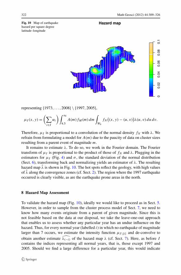
Fig. 10 Map of earthquakehazard per square degreelatitude–longitude

representing {1973, . . . ,2008} \ {1997,2005},

μI (x, y) =(∑

i∈I

αi

)∫ ∞

4.5A(m)fM(m)dm

∫

Wb

fN

((x, y) − (u, v)

)λ(u, v) dudv.

Therefore, μI is proportional to a convolution of the normal density fN with λ. Werefrain from formulating a model for A(m) due to the paucity of data on cluster sizesresulting from a parent event of magnitude m.

It remains to estimate λ. To do so, we work in the Fourier domain. The Fouriertransform of μI is proportional to the product of those of fN and λ. Plugging in theestimators for μI (Fig. 4) and σ , the standard deviation of the normal distribution(Sect. 6), transforming back and normalizing yields an estimator of λ. The resultinghazard map λ is shown in Fig. 10. The hot spots reflect the geology, with high valuesof λ along the convergence zones (cf. Sect. 2). The region where the 1997 earthquakeoccurred is clearly visible, as are the earthquake prone areas in the north.

8 Hazard Map Assessment

To validate the hazard map (Fig. 10), ideally we would like to proceed as in Sect. 5.However, in order to sample from the cluster process model of Sect. 7, we need toknow how many events originate from a parent of given magnitude. Since this isnot feasible based on the data at our disposal, we take the leave-one-out approachthat enables us to assess whether any particular year has an undue influence on thehazard. Thus, for every normal year (labelled i) in which no earthquake of magnitudelarger than 7 occurs, we estimate the intensity function μI\{i} and de-convolve to

obtain another estimate λ(−i) of the hazard map λ (cf. Sect. 7). Here, as before I

contains the indices representing all normal years, that is, those except 1997 and2005. Should we find a large difference for a particular year, this would indicate

Math Geosci (2012) 44:309–326 323

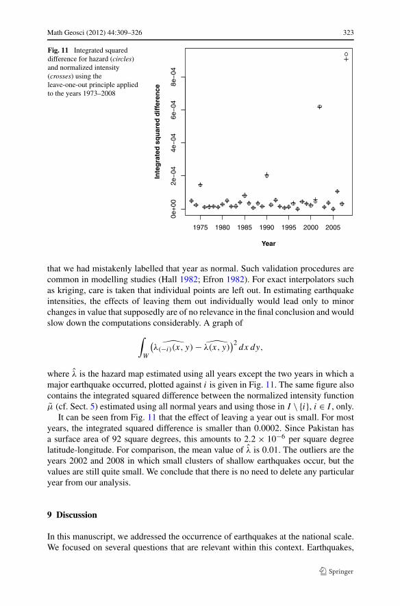
Fig. 11 Integrated squareddifference for hazard (circles)and normalized intensity(crosses) using theleave-one-out principle appliedto the years 1973–2008

that we had mistakenly labelled that year as normal. Such validation procedures arecommon in modelling studies (Hall 1982; Efron 1982). For exact interpolators suchas kriging, care is taken that individual points are left out. In estimating earthquakeintensities, the effects of leaving them out individually would lead only to minorchanges in value that supposedly are of no relevance in the final conclusion and wouldslow down the computations considerably. A graph of

∫

W

(λ(−i)(x, y) − λ(x, y)

)2dx dy,

where λ is the hazard map estimated using all years except the two years in which amajor earthquake occurred, plotted against i is given in Fig. 11. The same figure alsocontains the integrated squared difference between the normalized intensity functionμ (cf. Sect. 5) estimated using all normal years and using those in I \ {i}, i ∈ I , only.

It can be seen from Fig. 11 that the effect of leaving a year out is small. For mostyears, the integrated squared difference is smaller than 0.0002. Since Pakistan hasa surface area of 92 square degrees, this amounts to 2.2 × 10−6 per square degreelatitude-longitude. For comparison, the mean value of λ is 0.01. The outliers are theyears 2002 and 2008 in which small clusters of shallow earthquakes occur, but thevalues are still quite small. We conclude that there is no need to delete any particularyear from our analysis.

9 Discussion

In this manuscript, we addressed the occurrence of earthquakes at the national scale.We focused on several questions that are relevant within this context. Earthquakes,

324 Math Geosci (2012) 44:309–326

like most natural disasters, are not forced to have their effects in a single country,and we have included disasters that occurred across the different borders in our con-siderations, as much as these might have an effect in the country. With the adventof a more inter-regional approach, however, a similar analysis might be done whereattention focuses, for example, on a group of countries around one particular fault.Adversely, a similar analysis might be applicable as well to a region within a countrythat is particularly vulnerable.

An interesting issue that we discovered in passing when carrying out the analyseswas that the major shock in 2005 could be modelled in a more convincing way whenwe applied a double model. The major shock was followed by another large shock,and both generated aftershocks in an almost perfect way. The second shock and allits aftershocks could, alternatively, have been included as a set of aftershocks of thefirst event. This raises the issue at which stage one should distinguish a shock froman aftershock. Although these terms are intuitively clear, we were not successful infinding a sharp and unambiguous definition in the literature.

Relevant information such as population density could be taken into account, butthat was not available to us when carrying out the analysis. Similarly, the transitionof shock waves through the earth crust could serve to support the model that we ap-plied. This would also require additional data, in particular referring to the geologicalcomplexities. We felt that this was outside the scope of the current study, and maybe of little relevance as well when the emphasis would be on the support after theoccurrence of a disaster.

The approach described in the paper could be modified by including such addi-tional variation. There is also an interesting issue of data quality related to this study,i.e., the restriction to earthquakes of a magnitude larger than 4.5. It is reported inthe literature that earthquakes of a magnitude less than 4.5 are less well estimated.When studying the distribution of all earthquakes of size 4.0 and larger, we foundthat the histogram of the occurrences was deviating from the presumed exponentialmodel. Therefore, this theoretical model served as a tool to identify reliability ofthe observed earthquakes and thus confirmed that earthquakes of a lower magnitudewere less reliably recorded. A similar issue was raised when considering the depthsof occurrence of the earthquakes, where particular depths were occurring at a largefrequency. In fact the depths of 10 km occurred in nearly 30% of all earthquakes,the depth of 33 km in over 40%. For this reason, we did not include the depth of theearthquakes as a reliable parameter: Further studies have to show how depth relatedinformation can be included into the analysis.

10 Conclusions

This paper presents a range of tools to analyze the occurrence pattern of earthquakesat the national scale. The paper leads to several conclusions. First, a test has beendeveloped that allows one to check whether a pattern of point-like events (such asearthquakes) shows homogeneity through a range of years. This test has been basedupon the KPSS test statistic and for our data showed no indication of a spatial trendover the study period. Second, the inhomogeneous J -function has been applied for

Math Geosci (2012) 44:309–326 325

the first time to quantify spatial interaction in the apparently inhomogeneous patternof earthquakes within the borders of a single country. Even when accounting for non-homogeneity, additional clustering was found to be present. Third, a relatively stan-dard analysis of the aftershocks that occurred during two years of severe earthquakesin the country was carried out. We found that in one year a mixture of two majorshocks fitted the data better than a model in which all aftershocks arose from a sin-gle earthquake. Finally, a multivariate marked point process model was formulatedin which the components were Poisson cluster processes with normally distributedoffspring. A Fourier analysis of the spatial intensity of aggregated earthquakes wascarried out to obtain a hazard map. We found hot spots in the northern and mid-western parts of the country. In all, the modelling of earthquakes at the national levelof Pakistan turned out to be an exciting and relevant analysis of a spatio-temporalpoint pattern. We are convinced that much additional modelling can and should bedone, and that a proper interpretation of the derived results can lead to a careful man-agement of cities and infrastructure that may safe lives during future disasters.

Acknowledgements We are grateful to Ms. Salma Anwar, Mrs. Ellen-Wien Augustijn, and Mr. Markvan der Meijde at the Faculty of Geo-Information Science and Earth Observation of Twente Universitywho assisted us during the analysis. This research was done when the second author spent his sabbaticalleave at the Centre for Mathematics and Computer Science (CWI) in Amsterdam. He is grateful for thehospitality received during that period. This research was supported by The Netherlands Organisation forScientific Research NWO (613.000.809).

Calculations were done using the software package R. The libraries spatstat (Baddeley and Turner2005) and tseries (Trapletti and Hornik 2009) were especially useful.

Open Access This article is distributed under the terms of the Creative Commons Attribution Noncom-mercial License which permits any noncommercial use, distribution, and reproduction in any medium,provided the original author(s) and source are credited.

References

Adamopoulos L (1976) Cluster models for earthquakes: regional comparisons. Math Geol 8(4):463–475Adelfio G, Chiodi M (2010) Diagnostics for nonparametric estimation in space-time seismic processes.

J Environ Stat 1(2):1–13Adelfio G, Schoenberg FP (2009) Point process diagnostics based on weighted second order statistics and

their asymptotic properties. Ann Inst Stat Math 61(4):929–948Anwar S, Stein A, van Genderen JL (2012) Implementation of the marked Strauss point process model to

the epicenters of earthquake aftershocks. In: Shi W, Goodchild M, Lees B, Leung Y (eds) Advances ingeo-spatial information science. Taylor & Francis, London, pp 125–140. ISBN 978-0-415-62093-2

Baddeley A, Turner R (2005) Spatstat: an R package for analyzing spatial point patterns. J Stat Softw12(6):1–42

Baddeley AJ, Møller J, Waagepetersen R (2000) Non- and semi-parametric estimation of interaction ininhomogeneous point patterns. Stat Neerl 54(3):329–350

Besag J, Diggle PJ (1977) Simple Monte Carlo tests for spatial pattern. Appl Stat 26(3):327–333Daley DJ, Vere-Jones D (2003) An introduction to the theory of point processes. Volume I: Elementary

theory and methods, 2nd edn. Springer, New YorkDaley DJ, Vere-Jones D (2008) An introduction to the theory of point processes. Volume II: General theory

and structure, 2nd edn. Springer, New YorkDe Jong RM (2000) A strong consistency proof for heteroskedasticity and autocorrelation consistent co-

variance matrix estimators. Econom Theory 16(2):262–268Diggle PJ (1979) On parameter estimation and goodness-of-fit testing for spatial point patterns. Biometrics

35(1):87–101

326 Math Geosci (2012) 44:309–326

Diggle PJ (1985) A kernel method for smoothing point process data. Appl Stat 34(2):138–147Efron B (1982) The jackknife, the bootstrap, and other resampling plans. SIAM, PhiladelphiaGabriel E, Diggle PJ (2009) Second-order analysis of inhomogeneous spatio-temporal point process data.

Stat Neerl 63(1):43–51Gelfand AE, Diggle PJ, Fuentes M, Guttorp P (2010) Handbook of spatial statistics. CRC, Boca RatonHall P (1982) Cross-validation in density estimation. Biometrika 69(2):383–390Herrndorf N (1984) A functional central limit theorem for weakly dependent sequences of random vari-

ables. Ann Probab 12(1):141–153Holden L, Sannan S, Bungum H (2003) A stochastic marked point process model for earthquakes. Nat

Hazards Earth Syst Sci 2003(3):95–101Kwiatkowski D, Phillips PCB, Schmidt P, Shin Y (1992) Testing the null hypothesis of stationarity against

the alternative of a unit root. J Econom 54:159–178Lucio PS, De Brito NLC (2004) Detecting randomness in spatial point patterns: a “Stat-Geometrical”

alternative. Math Geol 36(1):79–99Molnar P, Chen WP (1982) Seismicity and mountain building. In: Hsu KJ (ed) Mountain building pro-

cesses. Academic Press, London, pp 41–58Newey WK, West KD (1987) A simple, positive semi-definite, heteroskedasticity and autocorrelation con-

sistent covariance matrix. Econometrica 55(3):703–708Ogata Y (1988) Statistical models for earthquake occurrences and residual analysis for point processes.

J Am Stat Assoc 83(401):9–27Ogata Y (1998) Space-time point-process models for earthquake occurrences. Ann Inst Stat Math

50(2):379–402Pei T (2011) A nonparametric index for determining the numbers of events in clusters. Math Geosci

43:345–362Pei T, Zhua AX, Zhou C, Li B, Qin C (2007) Delineation of support domain of feature in the presence of

noise. Comput Geosci 33:952–965Phillips PCB, Perron P (1988) Testing for a unit root in time series regression. Biometrika 75(2):335–346Shurygin AM (1993) Statistical analysis and long-term prediction of seismicity for linear zones. Math

Geol 25(7):759–772Stoyan D, Stoyan H (2000) Improving ratio estimators of second order point process characteristics. Scand

J Stat 27(4):641–656Trapletti A, Hornik K (2009) tseries: time series analysis and computational finance. R package version

0.10-22Van Lieshout MNM (2011) A J -function for inhomogeneous point processes. Stat Neerl 65(2):183–201Vere-Jones D (1970) Stochastic models for earthquake occurrence. J R Stat Soc B 32(1):1–62Vere-Jones D, Musmeci F (1992) A space-time clustering model for historical earthquakes. Ann Inst Stat

Math 44(1):1–11Zhuang J, Ogata Y, Vere-Jones D (2002) Stochastic declustering of space-time earthquake occurrences.

J Am Stat Assoc 97(458):369–380