the finite-difference modelling of earthquake motions
TRANSCRIPT


Trim: 247mm × 174mm Top: 14.762mm Gutter: 23.198mmCUUK2497-FM CUUK2497/Moczo ISBN: 978 1 107 02881 4 November 19, 2013 18:3
THE FINITE-DIFFERENCE MODELLING OFEARTHQUAKE MOTIONS
Waves and Ruptures
Numerical simulation is an irreplaceable tool in earthquake ground motion research. Among allthe numerical methods in seismology, the finite-difference (FD) technique is the most widely used,providing the best balance of accuracy and computational efficiency. Now, for the first time, this bookoffers a comprehensive introduction to this method and its applications to earthquake motion.
Using a systematic tutorial approach, the book requires only an undergraduate degree-level math-ematical background and provides a user-friendly explanation of the relevant theory. It explains FDschemes for solving wave equations and elastodynamic equations of motion in heterogeneous media,and provides an introduction to the rheology of viscoelastic and elastoplastic media. It also presents anadvanced FD time-domain method for efficient numerical simulations of earthquake ground motionin realistic complex models of local surface sedimentary structures, which are often responsible foranomalous earthquake motion and site effects in earthquakes.
Accompanied by a suite of online resources to help put the theory into practice, this is a vitalresource for professionals and academic researchers using numerical seismological techniques, andgraduate students in earthquake seismology, computational and numerical modelling, and appliedmathematics.
peter moczo is a professor of physics and Chair of the Department of Astronomy, Physics ofthe Earth, and Meteorology at Comenius University, Bratislava. He is the main author of severalmonographs and extended articles on the finite-difference method (including the seminal Acta PhysicaSlovaca article that partly forms the basis of this book). Professor Moczo is a member of theLearned Society of the Slovak Academy of Sciences, and his awards include the Prize of the SlovakAcademy of Sciences for Infrastructure, the Silver Medal of the Faculty of Mathematics, Physics andInformatics of Comenius University, and the Dionyz Stur Medal of the Slovak Academy of Sciencesfor Achievements in Natural Sciences.
Along with his two co-authors, Professor Moczo is a leading member of the (informal) NuQuakeresearch group, studying numerical modelling of seismic wave propagation and earthquake motion,at Comenius University and the Slovak Academy of Science in Bratislava. As part of this group, allthree authors were major contributors to the elaboration of the finite-difference method and hybridfinite-difference–finite-element method.
jozef kristek is an associate professor of physics at the Department of Astronomy, Physics of theEarth, and Meteorology at Comenius University, Bratislava. His research, as part of the NuQuakegroup, focuses on the development of numerical-modelling methods for seismic wave propagationand earthquake motion in structurally complex media, and Dr Kristek has been awarded the Prize ofthe Slovak Academy of Sciences for Infrastructure and the Dean’s Prize for Science for his work inthis area.
martin galis is a post-doctoral researcher at the King Abdullah University of Science and Tech-nology (KAUST), Saudi Arabia. Dr Galis’ research also focuses on the development of numerical-modelling methods for seismic wave propagation and earthquake motion in structurally complexmedia. He has also been awarded the Prize of the Slovak Academy of Sciences for Infrastructure.

Trim: 247mm × 174mm Top: 14.762mm Gutter: 23.198mmCUUK2497-FM CUUK2497/Moczo ISBN: 978 1 107 02881 4 November 19, 2013 18:3
Trim: 247mm × 174mm Top: 14.762mm Gutter: 23.198mmCUUK2497-FM CUUK2497/Moczo ISBN: 978 1 107 02881 4 November 19, 2013 18:3
THE FINITE-DIFFERENCEMODELLING OF
EARTHQUAKE MOTIONS
Waves and Ruptures
PETER MOCZOComenius University, Bratislava
andSlovak Academy of Sciences, Bratislava
JOZEF KRISTEKComenius University, Bratislava
MARTIN GALISKing Abdullah University of Science and Technology, Saudi Arabia
with contributions by
MIRIAM KRISTEKOVA, EMMANUEL CHALJUB,MARTIN KASER, PETER KLIN AND
CHRISTIAN PELTIES

Trim: 247mm × 174mm Top: 14.762mm Gutter: 23.198mmCUUK2497-FM CUUK2497/Moczo ISBN: 978 1 107 02881 4 November 19, 2013 18:3
University Printing House, Cambridge CB2 8BS, United Kingdom
Published in the United States of America by Cambridge University Press, New York
Cambridge University Press is part of the University of Cambridge.
It furthers the University’s mission by disseminating knowledge in the pursuit ofeducation, learning and research at the highest international levels of excellence.
www.cambridge.orgInformation on this title: www.cambridge.org/9781107028814
c© Peter Moczo, Jozef Kristek and Martin Galis 2014
This publication is in copyright. Subject to statutory exceptionand to the provisions of relevant collective licensing agreements,no reproduction of any part may take place without the written
permission of Cambridge University Press.
First published 2014
Printed in the United Kingdom by MPG Printgroup Ltd, Cambridge
A catalogue record for this publication is available from the British Library
Library of Congress Cataloguing in Publication dataMoczo, Peter, 1956– author.
The finite-difference modelling of earthquake motions : waves and ruptures / Peter Moczo, Comenius University,Bratislava and Slovak Academy of Sciences, Bratislava, Jozef Kristek, Comenius University, Bratislava, Martin
Galis, King Abdullah University of Science and Technology, Saudi Arabia ; with contributions by MiriamKristekova, Emmanuel Chaljub, Martin Kaser, Peter Klin and Christian Pelties.
pages cmIncludes bibliographical references and index.
ISBN 978-1-107-02881-4 (hardback)1. Seismology – Mathematical models. 2. Finite differences. I. Kristek, Jozef, author.
II. Galis, Martin, author. III. Title.QE539.2.M37M63 2014
551.2201′51562 – dc23 2013034912
ISBN 978-1-107-02881-4 Hardback
Additional resources for this publication at www.cambridge.org/moczo
Cambridge University Press has no responsibility for the persistence or accuracy ofURLs for external or third-party internet websites referred to in this publication,
and does not guarantee that any content on such websites is, or will remain,accurate or appropriate.

Trim: 247mm × 174mm Top: 14.762mm Gutter: 23.198mmCUUK2497-FM CUUK2497/Moczo ISBN: 978 1 107 02881 4 November 19, 2013 18:3
To Janulka, Mirka and Fibi

Trim: 247mm × 174mm Top: 14.762mm Gutter: 23.198mmCUUK2497-FM CUUK2497/Moczo ISBN: 978 1 107 02881 4 November 19, 2013 18:3

Trim: 247mm × 174mm Top: 14.762mm Gutter: 23.198mmCUUK2497-FM CUUK2497/Moczo ISBN: 978 1 107 02881 4 November 19, 2013 18:3
Contents
Acknowledgements page xvList of selected symbols xvii
1 Introduction 1
PART I MATHEMATICAL-PHYSICAL MODEL
2 Basic mathematical-physical model 72.1 Medium 72.2 Governing equation: equation of motion 8
2.2.1 Strong form 92.2.2 Weak form 102.2.3 Integral strong form 112.2.4 Concluding remark 11
2.3 Constitutive law: stress–strain relation 112.3.1 Elastic continuum 122.3.2 Viscoelastic continuum 13
2.4 Strong-form formulations of equations 132.4.1 Displacement–stress formulation 142.4.2 Displacement formulation 142.4.3 Displacement–velocity–stress formulation 142.4.4 Velocity–stress formulation 14
2.5 Boundary conditions 162.5.1 Free surface 162.5.2 Welded material interface 16
2.6 Initial conditions 172.7 Wavefield source (wavefield excitation) 17
3 Rheological models of a continuum 183.1 Basic rheological models 20
3.1.1 Hooke elastic solid 203.1.2 Newton viscous liquid 223.1.3 Saint-Venant plastic solid 22
vii

Trim: 247mm × 174mm Top: 14.762mm Gutter: 23.198mmCUUK2497-FM CUUK2497/Moczo ISBN: 978 1 107 02881 4 November 19, 2013 18:3
viii Contents
3.2 Combined rheological models 233.3 Viscoelastic continuum and its rheological models 23
3.3.1 Stress–strain and strain–stress relations in a viscoelasticcontinuum 24
3.3.2 Maxwell and Kelvin–Voigt bodies 273.3.3 Zener body (standard linear solid) 273.3.4 Phase velocity in elastic and viscoelastic continua 313.3.5 Measure of dissipation and attenuation in a viscoelastic
continuum 333.3.6 Attenuation in Zener body 353.3.7 Generalized Zener body 353.3.8 Generalized Maxwell body 383.3.9 Equivalence of GZB and GMB-EK 393.3.10 Anelastic functions (memory variables) 403.3.11 Anelastic coefficients and unrelaxed modulus 433.3.12 Attenuation and phase velocity in GMB-EK/GZB continuum 443.3.13 Stress–strain relation in 3D 45
3.4 Elastoplastic continuum 463.4.1 Simplest elastoplastic bodies 473.4.2 Iwan elastoplasic model for hysteretic stress–strain behaviour 50
4 Earthquake source 584.1 Dynamic model of an earthquake source 59
4.1.1 Boundary conditions for dynamic shear faulting 604.1.2 Friction law 61
4.2 Kinematic model of an earthquake source 644.2.1 Point source 654.2.2 Finite-fault kinematic source 68
PART II THE FINITE-DIFFERENCE METHOD
5 Time-domain numerical methods 735.1 Introduction 735.2 Fourier pseudo-spectral method 745.3 Spectral element method 765.4 Spectral discontinuous Galerkin scheme with ADER time integration 795.5 Hybrid methods 81
6 Brief introduction to the finite-difference method 836.1 Space–time grids 83
6.1.1 Cartesian grid 836.1.2 Uniform, nonuniform and discontinuous grids 846.1.3 Structured and unstructured grids 846.1.4 Space–time locations of field variables 84

Trim: 247mm × 174mm Top: 14.762mm Gutter: 23.198mmCUUK2497-FM CUUK2497/Moczo ISBN: 978 1 107 02881 4 November 19, 2013 18:3
Contents ix
6.2 FD approximations based on Taylor series 866.2.1 Simple approximations 866.2.2 Combined approximations: convolution 886.2.3 Approximations applied to a harmonic wave 906.2.4 General note on the FD approximations 91
6.3 Explicit and implicit FD schemes 936.4 Basic properties of FD schemes 946.5 Approximations based on dispersion-relation-preserving criterion 96
7 1D problem 977.1 Equation of motion and the stress–strain relation 977.2 A simple FD scheme: a tutorial introduction to FD schemes 99
7.2.1 Plane harmonic wave in a physical continuum 1007.2.2 Plane harmonic wave in a grid 1007.2.3 The (2,2) 1D FD scheme on a conventional grid 1017.2.4 Analysis of grid-dispersion relations 1037.2.5 Summary of the identified partial regimes 1147.2.6 Grid phase and group velocities 1157.2.7 Local error 1197.2.8 Sufficiently accurate numerical simulation 121
7.3 FD schemes for an unbounded smoothly heterogeneous medium 1237.3.1 (2,2) Displacement scheme on a conventional grid 1237.3.2 (2,2) Displacement–stress scheme on a spatially staggered grid 1257.3.3 (2,2) Velocity–stress scheme on a staggered grid 1277.3.4 Optimally accurate displacement scheme on a conventional grid 1297.3.5 (2,4) and (4,4) velocity–stress schemes on a staggered grid 1337.3.6 (4,4) Velocity–stress schemes on a collocated grid 144
7.4 FD schemes for a material interface 1517.4.1 Simple general consideration 1527.4.2 Hooke’s law and equation of motion for a welded interface 1537.4.3 Simple rheological model of a welded interface 1547.4.4 FD schemes 154
7.5 FD schemes for a free surface 1557.5.1 Stress imaging 1567.5.2 Adjusted FD approximations 157
7.6 Boundaries of the spatial grid 1587.6.1 Perfectly matched layer: theory 1597.6.2 Perfectly matched layer: scheme 160
7.7 Wavefield excitation 1617.7.1 Body-force term and incremental stress 1627.7.2 Wavefield injection based on wavefield decomposition 162
7.8 FD scheme for the anelastic functions of a smooth medium 163
Trim: 247mm × 174mm Top: 14.762mm Gutter: 23.198mmCUUK2497-FM CUUK2497/Moczo ISBN: 978 1 107 02881 4 November 19, 2013 18:3
x Contents
8 3D finite-difference schemes 1668.1 Formulations and grids 166
8.1.1 Displacement conventional-grid schemes 1668.1.2 Velocity–stress staggered-grid schemes 1678.1.3 Displacement–stress schemes on the grid staggered
in space 1688.1.4 Velocity–stress partly staggered-grid schemes 1688.1.5 Optimally accurate schemes 1698.1.6 Velocity–stress schemes on the collocated grid 170
8.2 Schemes on staggered, partly staggered, collocated andconventional grids 1708.2.1 (2,4) velocity–stress scheme on the staggered grid 1718.2.2 (2,4) velocity–stress scheme on the partly staggered grid 1728.2.3 (4,4) velocity–stress scheme on the collocated grid 1758.2.4 Displacement scheme on the conventional grid 175
8.3 Accuracy of FD schemes with respect to P-wave to S-wave ratio:analysis of local errors 1768.3.1 Equations and FD schemes 1768.3.2 Local errors 1828.3.3 The exact and numerical values of displacement in a grid 1838.3.4 Equivalent spatial sampling for the errors in amplitude and the
vector difference 1858.3.5 Essential summary based on the numerical investigation 1878.3.6 Interpretation of the errors 1878.3.7 Summary 192
8.4 Stability and grid dispersion of the VS SG (2,4) scheme 193
9 Velocity–stress staggered-grid scheme for an unbounded heterogeneousviscoelastic medium 1999.1 FD modelling of a material interface 1999.2 Stress–strain relation at a material interface 202
9.2.1 Planar interface parallel to a coordinate plane 2039.2.2 Planar interface in a general orientation 2059.2.3 Effective orthorhombic averaged medium 2069.2.4 Effective grid density 2089.2.5 Simplified approach with harmonic averaging of elastic moduli:
isotropic averaged medium 2099.3 Incorporation of realistic attenuation 210
9.3.1 Material interface in a viscoelastic medium 2109.3.2 Scheme for the anelastic functions for an isotropic averaged
medium 211

Trim: 247mm × 174mm Top: 14.762mm Gutter: 23.198mmCUUK2497-FM CUUK2497/Moczo ISBN: 978 1 107 02881 4 November 19, 2013 18:3
Contents xi
9.3.3 Scheme for the anelastic functions for an orthorhombic averagedmedium 212
9.3.4 Coarse spatial distribution of anelastic functions 2139.3.5 VS SG (2,4) scheme for a heterogeneous viscoelastic medium 215
10 Schemes for a free surface 21710.1 Planar free surface 217
10.1.1 Stress imaging in the (2,4) VS SG scheme 21810.1.2 Adjusted FD approximations in the (2,4) VS SG scheme 221
10.2 Free-surface topography 223
11 Discontinuous spatial grid 22711.1 Overview of approaches 22711.2 Two basic problems and general considerations 22911.3 Velocity–stress discontinuous staggered grid 230
11.3.1 Calculation of the field variables at the boundary of the finergrid in the overlapping zone 230
11.3.2 Calculation of the field variables at the boundary of the coarsergrid in the overlapping zone 231
11.3.3 Calculation of the field variables at the nonreflecting boundary 233
12 Perfectly matched layer 23412.1 Split formulation of the PML 23512.2 Unsplit formulation of the PML 23812.3 Summary of the formulations 23912.4 Time discretization of the unsplit formulation 239
13 Simulation of the kinematic sources 24213.1 Wavefield decomposition 24213.2 Body-force term 24213.3 Incremental stress 245
14 Simulation of dynamic rupture propagation 24614.1 Traction-at-split-node method 24714.2 Implementation of TSN in the staggered-grid scheme 25214.3 Initiation of spontaneous rupture propagation 256
15 Preparation of computations and a computational algorithm 259
PART III FINITE-ELEMENT METHOD AND HYBRIDFINITE-DIFFERENCE–FINITE-ELEMENTMETHOD
16 Finite-element method 26316.1 Weak form of the equation of motion 263
Trim: 247mm × 174mm Top: 14.762mm Gutter: 23.198mmCUUK2497-FM CUUK2497/Moczo ISBN: 978 1 107 02881 4 November 19, 2013 18:3
xii Contents
16.2 Discrete weak form of the equation of motion for an element 26516.3 Shape functions 26716.4 FE scheme for an element using the local restoring-force vector 27316.5 FE scheme for the whole domain using the global restoring-force vector 27816.6 Efficient computation of the restoring-force vector 28216.7 Comparison of formulations with the restoring force and stiffness matrix 28316.8 Essential summary of the FEM implementation 284
17 Traction-at-split-node modelling of dynamic rupture propagation 28517.1 Implementation of TSN in the FEM 28517.2 Spurious high-frequency oscillations of the slip rate 28817.3 Approaches to suppress high-frequency oscillations 290
17.3.1 Adaptive smoothing 29017.3.2 Kelvin–Voigt damping 29217.3.3 A-posteriori filtration 293
18 Hybrid finite-difference–finite-element method 29518.1 Computational domain 29518.2 Principle of the FD–FE causal communication 29618.3 Smooth transition zone with FD–FE averaging 29718.4 Illustrative numerical simulations using hybrid FD–FE method 29918.5 Potential improvement of the hybrid FD–FE method 300
PART IV FINITE-DIFFERENCE MODELLING OF SEISMICMOTION AT REAL SITES
19 Modelling of earthquake motion: Mygdonian basin 30719.1 Modelling of earthquake motion and real earthquakes by the FDM 30719.2 Mygdonian basin near Thessaloniki, Greece 308
19.2.1 Why the Mygdonian basin? – the E2VP 30819.2.2 The realistic model and implied challenges 30919.2.3 Comparative modelling for stringent canonical models 31219.2.4 Modelling for the realistic three-layered viscoelastic model 32019.2.5 Lessons learned from ESG 2006 and E2VP 322
Concluding remarks: search for the best scheme 324
Appendix A: Time–frequency misfit and goodness-of-fit criteria forquantitative comparison of time signals 327A.1 Characterization of a signal 327
A.1.1 Simplest characteristics 327A.1.2 Time–frequency decomposition 328
A.2 Comparison of signals 329A.2.1 TF envelope and phase differences 329A.2.2 Locally normalized and globally normalized criteria 329

Trim: 247mm × 174mm Top: 14.762mm Gutter: 23.198mmCUUK2497-FM CUUK2497/Moczo ISBN: 978 1 107 02881 4 November 19, 2013 18:3
Contents xiii
A.3 Comparison of three-component signals 330A.3.1 TF misfit criteria 331A.3.2 TF goodness-of-fit criteria 331
References 335Index 363

Trim: 247mm × 174mm Top: 14.762mm Gutter: 23.198mmCUUK2497-FM CUUK2497/Moczo ISBN: 978 1 107 02881 4 November 19, 2013 18:3
Trim: 247mm × 174mm Top: 14.762mm Gutter: 23.198mmCUUK2497-FM CUUK2497/Moczo ISBN: 978 1 107 02881 4 November 19, 2013 18:3
Acknowledgements
We are very grateful to all who directly or indirectly helped us to write this book.Over recent years, we had several friendly informal suggestions to write a book on
finite-difference modelling, but we finally decided to do so after physicist Vladimır Buzek,a chief editor of our Acta Physica Slovaca volume in 2007, suggested the book to CambridgeUniversity Press, and Jean Virieux encouraged us to accept the challenge and evaluated ourproposal. We thank both Vladimır and Jean for their vision, advice and encouragement.
We also thank three anonymous reviewers for constructive and helpful reviews of thebook proposal.
We are grateful to Emmanuel Chaljub for contributing the section on the spectral-elementmethod, Peter Klin for the section on the Fourier pseudo-spectral method, Martin Kaserand Christian Pelties for the section on the arbitrarily high order derivative – discontinuousGalerkin method, and Miriam Kristekova for the section on the time–frequency misfitcriteria. We also thank Emmanuel Chaljub and Florent De Martin for their SEM simulations,and Miriam Kristekova for calculating time–frequency goodness-of-fit criteria. We thankRafael Abreu for collaboration on stability analysis.
We specially thank our students Aneta Richterova, Svetlana Stripajova, ZuzanaMargocova and Filip Kubina. Aneta helped us to elaborate the section on the elastoplasticcontinuum. Aneta, Svetlana and Zuzana carefully and critically read the whole manuscript,corrected misprints and mistakes, and suggested several improvements to make the textmore student-friendly. Filip critically read the first half of Chapter 7.
We greatly appreciate the kind and constructive help of colleagues who found time intheir intense schedules to critically read parts of the manuscript and made suggestionsthat helped us to improve the book: Steve Day, Jean-Paul Ampuero, Pierre-Yves Bard,Emmanuel Chaljub, Wei Zhang, Eric Dunham, Rafael Abreu, Florent de Martin, MartinMai, Fabian Bonilla, Leila Etemadsaeed and Anders Petersson.
Over the years of elaboration of our finite-difference modelling we enjoyed discussionsand learned much from Jean Virieux, Michel Bouchon, Pierre-Yves Bard, Steve Day,Emmanuel Chaljub, Ralph Archuleta, Robert Geller, Johan Robertsson, Jacobo Bielak,Martin Kaser, Jean-Paul Ampuero, Heiner Igel, Andreas Fichtner, Robert Graves, ArbenPitarka, Wei Zhang, Rafael Abreu, Zhenguo Zhang, Leo Eisner, Richard Liska and othercolleagues. All that we learned helped us to create the concept and contents of the book.
xv

Trim: 247mm × 174mm Top: 14.762mm Gutter: 23.198mmCUUK2497-FM CUUK2497/Moczo ISBN: 978 1 107 02881 4 November 19, 2013 18:3
xvi Acknowledgements
We also enjoyed the creative and challenging environment of the international projects inwhich we had the opportunity to contribute and elaborate finite-difference modelling, andlearn from others. We thank Pierre-Yves Bard for coordinating our participation in ISMOD,SESAME, NERIES and NERA, Heiner Igel for SPICE and QUEST, Kyriazis Pitilakisfor EUROSEIS-RISK, Alexandros Savvaidis for ITSAK-GR, and Fabrice Hollender forE2VP and SIGMA. Several results presented in the book were obtained within projectsOPTIMODE and MYGDONEMOTION funded by the Slovak grant agency APVV.
Some of the calculations were performed in the Computing Centre of the SlovakAcademy of Sciences using the supercomputing infrastructure acquired in project ITMS26230120002 and 26210120002 (Slovak infrastructure for high-performance computing)supported by the Research & Development Operational Programme funded by the ERDF.
We gladly acknowledge our colleagues Andrej Cipciar, Kristian Csicsay, LuciaFojtıkova, Robert Kysel, Klara Rampasekova, Miroslav Srbecky and Sebastian Sevcıkfor their kind support of our numerical-modelling research. We specially acknowledgeJozef Masarik for his valuable support of our research.
We also thank our editors at Cambridge University Press, Susan Francis, Laura Clarkand Rachel Cox, for their kind, patient and constructive help in preparation of the book.
We devote this book to our wives for their love, understanding and support.

Trim: 247mm × 174mm Top: 14.762mm Gutter: 23.198mmCUUK2497-FM CUUK2497/Moczo ISBN: 978 1 107 02881 4 November 19, 2013 18:3
Selected symbols
Abbreviations
AFDA adjusted finite-difference approximation techniqueCG conventional gridD displacement formulation (does not apply to abbreviations 2D or 3D)DS displacement–stress formulationDVS displacement–velocity–stress formulationDRP dispersion-relation-preservingEQ partial differential equationFD finite-differenceFDEQ finite-difference equationFDM finite-difference methodFDTD finite-difference time-domain methodFE finite-elementFEM finite-element methodGMB-EK generalized Maxwell body (Emmerich and Korn 1987)GZB generalized Zener bodyl.h.s. left hand side (of equation)PML perfectly matched layerr.h.s. right hand side (of equation)SEM spectral-element methodSG staggered gridPSG partly staggered gridTSN traction-at-split-nodeVS velocity–stress formulation
Mathematical notation
Dax ◦Dbx ≡ Dabx convolution of operatorsF , F−1 direct and inverse Fourier transforms
xvii

Trim: 247mm × 174mm Top: 14.762mm Gutter: 23.198mmCUUK2497-FM CUUK2497/Moczo ISBN: 978 1 107 02881 4 November 19, 2013 18:3
xviii List of selected symbols
x(t) ∗ y(t) convolution of functions
dj
dξjj-th total derivative with respect to ξ
∂j
∂ξ jj-th partial total derivative with respect to ξ
ϕi,j concise notation of spatial partial derivativeϕ concise notation of temporal partial derivative
Greek symbols
α P-wave speed attenuation coefficient (Subsection 3.3.5)α grid P-wave velocityβ S-wave speedβ grid S-wave velocityδ(t) Dirac delta functionδij Kronecker deltaδM modulus defect (relaxation of modulus)� time step�x,�y,�z grid spacingsε, εij 1D strain, strain tensor�ε strain vectorεkji Levi-Civita symbolζl(t) anelastic function for velocity–stress formulationζ (ω), ζ pij (ω) auxiliary functions for 1D and 3D PMLθ (ω), θpi (ω) auxiliary functions for 1D and 3D PMLκ bulk modulusλ Lame constant wavelengthμ shear modulus (Lame constant)μf coefficient of frictionμs , μd static and dynamic coefficients of frictionξl(t) anelastic function for displacement formulationsρ densityρAI effective grid densityσ , σij 1D stress, stress tensor�σ stress vectorτ0, τn initial and normal tractionsτd , τs dynamic and static frictional shear tractionsϕmI,K,L, �mI,K,L exact and approximate values of function ϕ at the grid point
(xI , yK, zL, tm)ω angular frequencyω grid angular frequency

Trim: 247mm × 174mm Top: 14.762mm Gutter: 23.198mmCUUK2497-FM CUUK2497/Moczo ISBN: 978 1 107 02881 4 November 19, 2013 18:3
List of selected symbols xix
ωl characteristic frequency�ref reference element
Latin symbols
c phase velocitycijkl tensor of elastic constantsDc characteristic (critical) slip-weakening distanceD(1−2)x , D(1−4)
x operators for the 2nd-order and 4th-order approximations ofthe 1st x -derivative
DFx , DBx forward and backward approximation of the 1st derivativeh grid spacing in the uniform gridI , K , L spatial grid-point indicesm time-level indexM0 scalar seismic moment�n, nj normal vectorO(hn) order of a remainder in Taylor seriesp stability ratioQ quality factorr VP /VS ratio�s slip�s slip rate (slip velocity)S surface (Section 2.2)
frictional strength / fault friction (Sections 4.1,14.1, 17.1)fault surface (Section 4.2)stability factor (Courant number) (Chapter 7)strength parameter (Section 14.3)
t timetm time at time level mT periodT mI±1/2 discrete approximation of stressTXX, TYY , TZZ, TXY , discrete grid values of the stress-tensor componentsTYZ, TZX�u, ui , ux , uy , uz displacementUmI discrete approximation of displacementUX, UY discrete grid values of the displacement-vector componentsv grid phase velocityvG grid group velocityvU grid phase velocity of the unstable wave�v, vi , vx , vy , vz particle velocity

Trim: 247mm × 174mm Top: 14.762mm Gutter: 23.198mmCUUK2497-FM CUUK2497/Moczo ISBN: 978 1 107 02881 4 November 19, 2013 18:3
xx List of selected symbols
V mI discrete approximation of the particle velocityVX, V Y , VZ discrete grid values of the particle velocityVP , VS P-wave speed, S-wave speedYl , Y κl , Yμl , Yαl , Yβl , Yλl anelastic coefficients(xI , yK , zL) spatial grid-point coordinates

Trim: 247mm × 174mm Top: 14.762mm Gutter: 23.198mmCUUK2497-01 CUUK2497/Moczo ISBN: 978 1 107 02881 4 November 14, 2013 14:44
1
Introduction
A tectonic earthquake is a unique, interesting and challenging natural phenomenon. At thesame time the earthquake can cause death and huge material losses. The Emilia-Romagna,Italy (moment magnitude Mw = 5.9, May 20, 2012), Tohoku-Oki, Japan (Mw = 9.0, March3, 2011), Christchurch, New Zealand (Mw = 6.3, February 22, 2011), Chile (Mw = 8.8,February 27, 2010), Port-au-Prince, Haiti (Mw = 7.0, January 12, 2010), L’Aquila, Italy(Mw = 6.3, April 6, 2009), Sichuan, China (Mw = 7.9, May 12, 2008), Pisco, Peru (Mw =8.0, August 15, 2007), Kashmir, Pakistan (Mw = 7.6, October 8, 2005), Sumatra, Indonesia(Mw = 9.1, December 26, 2004), Bam, Iran (Mw = 6.6, December 26, 2003), Gujarat,India (Mw = 7.7, January 26, 2001), Izmit, Turkey (Mw = 7.6, August 17, 1999), Kobe,Japan (Mw = 6.8, January 17, 1995), and Northridge, California (Mw = 6.7, January 17,1994) earthquakes are well-known examples of tragic and catastrophic events of the pasttwo decades. Three of them belong to the largest earthquakes ever recorded. Some ofthem, however, indicate a troubling and important fact: an earthquake that kills and causeslarge material damage is not necessarily a big event in terms of released energy. The Mw
6.7 Northridge 1994 and Mw 6.8 Kobe 1995 earthquakes caused, at the time, unprecedentedrecord economic losses in the USA and Japan, respectively, although they released (inthe form of seismic waves) roughly 3000 times less energy than the Mw 9.0 Tohoku-Oki 2011 earthquake. In the long-term average, there are approximately 13 earthquakesin the magnitude range [7, 7.9] and 120 in the magnitude range [6, 6.9] per year. Anyearthquake of this size can become a tragic and damaging event if it hits a densely populatedarea.
Apparently surprisingly, a significant part of the world’s population lives in earthquake-prone areas: large populated areas are close to active seismogenic faults, and, moreover,large cities are often located at the surface of sediment-filled basins and valleys. The reasonswhy large human settlements developed in such areas relate to the geology, hydrology,climate and geography of the areas and regions. Both aspects of the locations of large cities,that is, being close to seismogenic faults and atop sediments, have strong impacts on theearthquake hazard and consequently also earthquake risk. Being close to a seismogenic faultobviously poses an earthquake threat. Also being atop a sediment-filled basin or valley canconsiderably increase the earthquake hazard. This is because seismic wave interference andresonant phenomena in sediment-filled basins and valleys can produce anomalously large
1

Trim: 247mm × 174mm Top: 14.762mm Gutter: 23.198mmCUUK2497-01 CUUK2497/Moczo ISBN: 978 1 107 02881 4 November 14, 2013 14:44
2 Introduction
earthquake motion at the Earth’s surface and lead to so-called ‘site effects’; characteristics ofthe earthquake vibratory motion of the Earth’s surface can attain locally anomalous values –e.g., amplitudes can be considerably amplified in the time or frequency domain, and strongmotion can be significantly prolongated. The anomalous values can occur at frequencies atwhich buildings, constructions and industrial facilities can be damaged or destroyed. Thegreatest damage to buildings and constructions is often due to mutual resonance betweenthe local geological and artificial structures. The September 19, 1985 Mexico quake isone of the best examples of the damaging potential of such effects. The epicentre was onthe Pacific coast; however, the earthquake caused major damage in Ciudad de Mexico –more than 350 km away from the epicentre. A major part of the Mexican capital sitson unconsolidated lake sediments and artificial land or, in other words, atop a very softsedimentary basin. The interference and resonant phenomena in sediments led to disastrouseffects. Hundreds of buildings were completely destroyed, hundreds partially collapsed orwere seriously damaged. At least 10 000 people died.
In the worldwide long-term average, the number of earthquakes will not decrease. Onthe other hand, the density of population will increase in many areas. In industrializednations the technological complexity of the populated areas will increase. This could bringmore vulnerability to earthquakes if building codes are not either at the state-of-the-artlevel or actually enforced. In developing countries the increasing population means greatand growing earthquake risk. Even relatively weak earthquakes will be capable of causingtremendous human losses and damage, and consequently significantly affect the economyof the region or the entire country.
Two natural scientific tasks for seismologists are, therefore, earthquake prediction andprediction of ground motion during future earthquakes at a site of interest. These tasks arealso primary scientific responsibilities of seismologists towards society.
Seismologists still cannot predict the time, place and size of future earthquakes. Evenmore interestingly, we still do not know whether such prediction is possible in principleand will be possible technically. This is because we still do not have answers to importantquestions regarding the processes of the long-term preparation and nucleation of earth-quakes. We still do not know enough about seismogenic faults and the Earth’s interior atdepths where earthquakes are being prepared. This is mainly because we cannot simplyinstall sensors and instruments at those depths and places. In other words, a classical directcontrolled physical experiment aiming to measure these processes is impossible – at leastfrom an economic viewpoint at present. Direct measurements are practically restricted tothe Earth’s surface, and almost all information about the rupture process and structure ofthe Earth’s interior is encoded in instrument records of earth motion (seismograms) duringearthquakes. Consequently, our knowledge of the earthquake source and the Earth’s interiorhas to be confronted with the seismograms.
Hereby, we come to the role of theoretical and numerical-modelling methods. They areirreplaceable tools in earthquake research – in investigating preparation and nucleation ofearthquakes, the rupture process on the fault, radiation of seismic waves, seismic wavepropagation in the Earth’s interior, and earthquake motion of the Earth’s surface.

Trim: 247mm × 174mm Top: 14.762mm Gutter: 23.198mmCUUK2497-01 CUUK2497/Moczo ISBN: 978 1 107 02881 4 November 14, 2013 14:44
Introduction 3
No matter whether seismologists can or cannot timely predict earthquake occurrence,they must predict earthquake ground motion during potential future earthquakes in denselypopulated areas and sites of special importance, e.g., sites of nuclear power plants, bigdams and key industrial facilities. Even if the timely prediction of earthquake occurrencewere physically possible and technically feasible, seismologists must predict what canor will happen during a future earthquake. This is vital for land-use planning, designingnew buildings and reinforcing existing ones. It is also extremely important for undertakingactions that could help mitigate losses during future earthquakes.
Prediction of the earthquake ground motion for a given area or site might be based on anempirical approach if sufficient earthquake recordings at the site or physically relevant forthe site were available. In most cases, however, there is a severe lack of data. Consequently,it is the theory and numerical simulations that have to be applied.
Although we still need to better understand processes in the Earth and considerably betterknow the Earth’s interior and seismogenic faults, the present state of our knowledge andthe capabilities of modern seismic arrays impose stringent requirements on the theoreticaland computational models. For example, considering computational models of surfacelocal geological structures, it is necessary to include nonplanar interfaces between layers –possibly with large contrasts in values of material parameters, gradients in P-wave andS-wave speeds, density and quality factors inside layers, P-wave to S-wave speed ratiopossibly as large as 5 and more in the soft surface sediments, and often also free-surfacetopography. In particular, the rheology of the medium has to allow for realistic broad-band attenuation. Realistic strong ground motion simulations should also account for thepossibility of nonlinear behaviour in soft soils.
There are no exact (analytical) solutions for such realistic models. Only approximatecomputational methods are able to account for the geometrical and rheological complexityof the sufficiently realistic models. The most important aspects of all methods are accuracyand computational efficiency (in terms of computer memory and time). These two aspectsare in most cases contradictory. It is, however, the reasonable balance between the accuracyand computational efficiency in the case of complex realistic structures that makes thenumerical-modelling methods and, more specifically, so-called domain (in the spatial sense)numerical methods dominant among all approximate methods.
A variety of domain numerical methods have been developed in application to earthquakemotion during the past few decades. The best known are the (time-domain) finite-difference,finite-element, Fourier pseudo-spectral, spectral-element and discontinuous Galerkin meth-ods. Both theoretical analyses and numerical experience show that none of these methodscan be chosen as the universally best (in terms of accuracy and computational efficiency)method for all important problems in earthquake research, that is, for all medium-wavefieldconfigurations. Each method has its advantages and disadvantages, which often depend onthe particular application.
Moreover, recent experience from two international comparative numerical exercisesfor the Grenoble valley, France, and the Mygdonian basin near Thessaloniki, Greece (ESG2006 and E2VP, respectively), show that at least two different but comparably accurate
Trim: 247mm × 174mm Top: 14.762mm Gutter: 23.198mmCUUK2497-01 CUUK2497/Moczo ISBN: 978 1 107 02881 4 November 14, 2013 14:44
4 Introduction
methods should be used in order to obtain a reliable numerical prediction of earthquakeground motion for a site of interest.
Two decades of 3D earthquake motion modelling, mainly in California, the SCEC com-parative exercises, ESG 2006 and E2VP confirmed that, despite development of alternativeand new methods, the FD time-domain method has an important and, without hesitationand exaggeration, irreplaceable position and role among recent time-domain numerical-modelling methods in earthquake research.
It is important to say that the term ‘finite-difference method’(FDM) in the numericalmodelling of earthquake motion may represent one out of a large number of various FDschemes and codes. The schemes may considerably differ from each other in severalmethodological aspects. Consequently, the schemes and the numerical results obtained bydifferent schemes may differ considerably in accuracy and computational efficiency.
The most advanced FD schemes can be more than competitive, for many important con-figurations, with other modern methods: at the same level of accuracy they can be compu-tationally more efficient. For some configurations, other methods can be more appropriate.
More than four decades of development of the fFDM in application to seismic wavepropagation and earthquake motion, and the present state of FD theory suggest that there isroom for further improvements, and that the future will bring even more accurate, efficientand competitive schemes for geometrically and rheologically complex realistic problemconfigurations.
In this book we focus on the FDM as applied to modelling earthquake motion andearthquake ground motion prediction. Obviously, the included material also reflects ourcontributions to the methodology of FD modelling. Due to the chosen focus and limitedextent, we do not cover all aspects of FD modelling. At the same time, we believe that thebook brings material that will be found useful by those who are not familiar with the method(students, professionals, researchers) and also those who develop and apply numericalmodelling in their earthquake research or investigations of elastic wave propagation incomplex media (e.g., oil exploration, shallow geophysics, machine-induced vibrations).

Trim: 247mm × 174mm Top: 14.762mm Gutter: 23.198mmCUUK2497-02 CUUK2497/Moczo ISBN: 978 1 107 02881 4 November 14, 2013 15:21
Part IMathematical-physical model

Trim: 247mm × 174mm Top: 14.762mm Gutter: 23.198mmCUUK2497-02 CUUK2497/Moczo ISBN: 978 1 107 02881 4 November 14, 2013 15:21

Trim: 247mm × 174mm Top: 14.762mm Gutter: 23.198mmCUUK2497-02 CUUK2497/Moczo ISBN: 978 1 107 02881 4 November 14, 2013 15:21
2
Basic mathematical-physical model
In this chapter we briefly present the basics of the mathematical-physical model neces-sary for the explanations and elaborations in the following chapters. For more detailedexpositions of the theory of earthquakes, seismic wave propagation and earthquake groundmotion we refer to some of the recent monographs and fundamental textbooks. For a generalintroduction to seismology – Aki and Richards (2002), Pujol (2003), Shearer (2009), Steinand Wysession (2003), Lay and Wallace (1995), Kennett (2001), Beroza and Kanamori(2009), Dziewonski and Romanowicz (2009); for earthquake sources – Kostrov and Das(2005), Scholz (2002), Ohnaka (2013); for theory of seismic wave propagation – Ben-Menahem and Singh (2000) and Carcione (2007); for global seismic wave propagation –Dahlen and Tromp (1998); for full waveform modelling and inversion – Fichtner (2011);for geotechnical earthquake engineering – Kramer (1996); and for waves and vibrations insoils caused by earthquakes, traffic, shocks and construction works – Semblat and Pecker(2009).
2.1 Medium
In order to reasonably numerically simulate seismic wave propagation and earthquakemotion in the Earth we need an adequate model of the medium inside a target domain(volume) of the Earth. We should clearly distinguish geological models, physical modelsand discrete (or grid) models.
In general, a physical model of a medium is described by 3D distributions of all materialparameters that determine seismic wave propagation and earthquake motion. Being focusedon seismic and earthquake motion in near-surface local structures, in most cases the realmaterial can be modelled as a heterogeneous linear viscoelastic isotropic continuum. Mod-els of the medium may comprise both spatially smooth and discontinuous variations ofmaterial parameters. The model has to properly account for attenuation due to anelasticityof the Earth’s real material. A perfectly elastic medium or oversimplified description ofattenuation is not sufficient. A reasonable rheological viscoelastic model is necessary inorder to account for the realistic dependence of attenuation on frequency and its spatialvariations.
7

Trim: 247mm × 174mm Top: 14.762mm Gutter: 23.198mmCUUK2497-02 CUUK2497/Moczo ISBN: 978 1 107 02881 4 November 14, 2013 15:21
8 Basic mathematical-physical model
So far, the least addressed aspect in numerical modelling of earthquake motion in near-surface local structures is the (an)isotropy of the real material. We know, in general, thatthere are true isotropic materials and true anisotropic materials. The question is, what canbe seen in seismic records? For example, anisotropy of the Earth’s upper mantle is clearlyobserved in seismic records, and numerical modelling of seismic waves at the regional andglobal scales has to assume inherent physical anisotropy. We are not in such a situation innumerical modelling of earthquake motion in near-surface local structures.
Although the real medium and its physical model may consist of truly isotropic materials,the mathematical-physical and grid representations of wave propagation in such a mediummay be anisotropic. We may speak, for instance, of an equivalent anisotropic medium in thecase of a low-frequency approximation (wavelengths much larger than the characteristicsize of heterogeneity) for wave propagation in heterogeneous isotropic media (Backus1962, Helbig 1984).
The usual physical model of the medium is specified by 3D spatial distributions of theP-wave and S-wave speeds (VP or α, and VS or β, respectively) at some frequency, density(ρ), and P-wave and S-wave quality factors as functions of frequency (QP(ω) and QS(ω),respectively).
Soft sediments near the free surface may behave in a nonlinear fashion. The stress–strain relation is not linear but nonlinear hysteretic. In the simplest (but still tremendouslydemanding) case the medium has to be represented by a rheological elastoplastic model.This poses a major complication for 3D modelling of earthquake motion. At present,reasonable 3D numerical modelling with possibly nonlinear behaviour of part of the wholemodel is still a challenge for numerical modellers.
Plastic deformation in the close vicinity of a rupturing fault is another example ofnonlinear behaviour that is not trivial to model numerically.
2.2 Governing equation: equation of motion
Consider a material volume V of continuum with surface S. Material parameters are contin-uous functions of spatial coordinates inside V. Consider an arbitrary volume�with surfaceS� inside volume V. Let �n� be a normal vector to surface S� pointing from the interior ofvolume � outward. Let �f (xk, t) be the density of the body force acting in volume � and�T �(xk, t) the traction acting at surface S�. Here xk; k ∈ {1, 2, 3} are Cartesian coordinatesand t is time. The configuration is shown in Fig. 2.1. Let �u (u1, u2, u3) or, in an alternativenotation, �u (ux, uy, uz), be the displacement vector. Let εij be the strain tensor,
εij = 1
2
(∂ui
∂xj+ ∂uj∂xi
); i, j ∈ {1, 2, 3} (2.1)
and σij the stress tensor. We briefly introduce the basic forms of the equations of motionfor the considered configuration.

Trim: 247mm × 174mm Top: 14.762mm Gutter: 23.198mmCUUK2497-02 CUUK2497/Moczo ISBN: 978 1 107 02881 4 November 14, 2013 15:21
2.2 Governing equation: equation of motion 9
T Ω
TSΩ
Ω
Figure 2.1 Material volume V of a smooth continuum bounded by surface S. External traction �T actsat surface S, body force �f acts in volume V. Volume�with surface S� is a testing volume consideredin the derivation of the equation of motion.
In the following formulations, the traction vector appears explicitly, which means thepossible imposition of the Neumann boundary condition on a surface. The possible appli-cation of the Dirichlet boundary condition (prescribed displacement) does not explicitlyappear in the formulations.
2.2.1 Strong form
An application of Newton’s second law to volume � gives
d
dt
∫�
ρ∂ui
∂tdV =
∫S�T �i dS +
∫�
fidV (2.2)
Throughout the text dV and dS will be used for volume and surface elements, respectively.Because � and S� move with particles, the particle mass ρdV does not change with time.The equation can be written as∫
�
ρ∂2ui
∂t2dV =
∫S�T �i dS +
∫�
fidV (2.3)
At surface S�, traction T �i is related to the stress tensor σij :
T �i = σijn�j (2.4)
In Eq. (2.4) and hereafter we assume the Einstein summation convention for repeatedindices. Assuming continuity of the stress tensor throughout volume�, Gauss’s divergencetheorem can be applied to the surface integral:∫
S�T �i dS =
∫S�σijn
�j dS =
∫�
∂σij
∂xjdV (2.5)

Trim: 247mm × 174mm Top: 14.762mm Gutter: 23.198mmCUUK2497-02 CUUK2497/Moczo ISBN: 978 1 107 02881 4 November 14, 2013 15:21
10 Basic mathematical-physical model
Equation (2.3) can be then written as∫�
(ρ∂2ui
∂t2− ∂σij∂xj
− fi)dV = 0 (2.6)
Equation (2.6) is valid for any volume� inside V. Assume that the integrand is greater than0 at some point inside V. Because the integrand is continuous throughout V, it is possibleto find such a volume � (containing that point) for which the integrand is greater than 0.This, however, would be in contradiction with Eq. (2.6). Consequently,
ρ∂2ui
∂t2− ∂σij∂xj
− fi = 0 (2.7)
everywhere in V. Equation (2.7) together with the boundary condition at surface S,
Ti = σijnj (2.8)
represent a strong formulation for the considered problem. The formulation requires con-tinuity of displacement and its first spatial derivatives.
2.2.2 Weak form
Alternatively to the application of Newton’s second law to the material volume V wecan apply the principle of virtual work. Consider a fixed state of continuum at sometime and its virtual (arbitrary, infinitesimal) deformation. Let δui be the correspondingvirtual displacement. Then the virtual deformation is characterized by the virtual straintensor δεij :
δεij = 1
2
[∂
∂xjδui + ∂
∂xiδuj
](2.9)
Because the virtual displacements are assumed in a fixed state of continuum, they do notaffect displacements and accelerations of continuum particles in this state. The principlestates that during virtual deformation the work done by external forces has to be equal tothe sum of the increment of energy of deformation and the work of inertial forces:∫
S
TiδuidS +∫V
fiδuidV =∫V
σij δεij dV +∫V
ρ∂2ui
∂t2δuidV (2.10)
Functions δui are arbitrary; they are equivalent to weight functions. Therefore, we replaceδui by wi in Eqs. (2.9) and (2.10). Then, due to symmetry of the stress tensor,
σij δεij = 1
2
(σij∂wi
∂xj+ σij ∂wj
∂xi
)= σij ∂wi
∂xj(2.11)
Equation (2.10) can be written as∫V
(ρ∂2ui
∂t2− fi
)widV +
∫V
σij∂wi
∂xjdV =
∫S
TiwidS (2.12)

Trim: 247mm × 174mm Top: 14.762mm Gutter: 23.198mmCUUK2497-02 CUUK2497/Moczo ISBN: 978 1 107 02881 4 November 14, 2013 15:21
2.3 Constitutive law: stress–strain relation 11
Equation (2.12) is called the weak form of the equation of motion. This is because therequirement of continuity of displacement and its first spatial derivatives in the strong formis replaced here by a weaker requirement of continuity of displacement and the weightfunctions.
2.2.3 Integral strong form
Integration by parts of the last term on the left hand side (l.h.s.) of Eq. (2.12) yields∫V
(ρ∂2ui
∂t2− fi
)widV +
∫V
∂
∂xj
(σijwi
)dV −
∫V
∂σij
∂xjwidV =
∫S
TiwidS (2.13)
and, using Gauss’s divergence theorem,∫V
(ρ∂2ui
∂t2− fi
)widV +
∫S
σijnjwidS −∫V
∂σij
∂xjwidV =
∫S
TiwidS (2.14)
Assembling the volume and surface integrals together gives∫V
(ρ∂2ui
∂t2− ∂σij∂xj
− fi)widV =
∫S
(Ti − σijnj
)widS (2.15)
In Eq. (2.15) we can specify the boundary condition for traction at surface S by specifyingvalues of Ti . We can call Eq. (2.15) the integral strong form of the equation of motion(we adopted this term based on our personal communication with Robert J. Geller). Whilebeing integral, the form requires continuity of the first derivative of displacement. Thesetwo features clearly distinguish it from the (differential) strong form and the integral weakform.
2.2.4 Concluding remark
In principle, any of the three forms can be the basis for discretization aiming in an FDscheme. Most of the developed FD schemes are based on the differential strong form –likely due to its apparent relative simplicity. Depending on the problem configuration, oneof the two other forms may be found more suitable. The weak form is the basis for thetraditional FEM, the more recent spectral-element method and the discontinuous Galerkinmethod. These methods will be briefly characterized in Chapter 5.
2.3 Constitutive law: stress–strain relation
In order to solve the equation of motion we need a constitutive law that specifies therelation between the stress and strain tensors, and consequently also the relation betweenthe stress tensor and displacement vector. We will consider three types of continuum –linear elastic, linear viscoelastic and nonlinear elastoplastic. The linear elastic continuumis the simplest type of continuum. It is useful for a simple introduction of many importantconcepts and approaches but is incapable of accounting for attenuation of seismic waves

Trim: 247mm × 174mm Top: 14.762mm Gutter: 23.198mmCUUK2497-02 CUUK2497/Moczo ISBN: 978 1 107 02881 4 November 14, 2013 15:21
12 Basic mathematical-physical model
and motion. Realistic attenuation can be reasonably accounted for by the viscoelasticmedium. Eventually we also describe the simplest elastoplastic continuum in order toaccount for the hysteretic stress–strain relation in surface soft sediments. Rheologicalmodels of a continuum will be addressed in detail in Chapter 3. Here we concisely presentthe fundamental relations for the elastic and viscoelastic continua.
2.3.1 Elastic continuum
Cauchy’s generalization of the original Hooke’s law in tensor form reads
σij = cijklεkl (2.16)
where cijkl is a tensor of elastic constants (they are constant with respect to the strain-tensorcomponents, not necessarily with respect to spatial position). Equation (2.16) assumes thateach stress-tensor component is a linear combination of all components of the strain tensor.Symmetry of the stress tensor and application of the first law of thermodynamics implysymmetries
cijkl = cjikl, cijkl = cklj i (2.17)
respectively. They yield additional symmetry
cijkl = cjilk (2.18)
Symmetries (2.17) and (2.18) reduce from 81 down to 21 the number of independent elasticconstants that describe the most general anisotropic medium. The situation dramaticallysimplifies in the case of an isotropic medium. The stress–strain relation of an isotropicelastic medium is described by two independent elastic constants. The stress–strain relationcan be written in the form
σij = κεkkδij + 2μ(εij − 1
3εkkδij)
(2.19)
where κ and μ are bulk and shear moduli, respectively, and
δij = 1; i = j δij = 0; i = j (2.20)
defines the Kronecker delta. Equation (2.19) corresponds to decomposition of the stresstensor into dilatational and deviatoric components. Alternatively, using
κ = λ+ 23μ (2.21)
the stress–strain relation can be written using Lame constants λ and μ in the form
σij = λεkkδij + 2μεij (2.22)
or as
σij = λ∂uk∂xkδij + μ
(∂ui
∂xj+ ∂uj∂xi
)(2.23)
Trim: 247mm × 174mm Top: 14.762mm Gutter: 23.198mmCUUK2497-02 CUUK2497/Moczo ISBN: 978 1 107 02881 4 November 14, 2013 15:21
2.4 Strong-form formulations of equations 13
2.3.2 Viscoelastic continuum
The stress–strain relation in a viscoelastic medium can be defined as
σij (t) =∫ t
−∞ψijkl (t − τ )
∂εkl (τ )
∂tdτ (2.24)
where ψijkl is a tensor of relaxation functions describing the behaviour of the material. Analternative form of the stress–strain relation is
εij (t) =∫ t
−∞χijkl (t − τ )
∂σkl (τ )
∂tdτ (2.25)
where χijkl is a tensor of creep functions.For an isotropic medium the stress–strain relation can be written as
σij (t) = δij∫ t
−∞ψκijkl (t − τ )
∂εkk (τ )
∂tdτ
(2.26)
+ 2∫ t
−∞ψμijkl (t − τ )
[∂εkl (τ )
∂t− 1
3
∂εkk (τ )
∂tδij
]dτ
where ψκijkl and ψμijkl are relaxation functions for the bulk and shear moduli, respectively.Alternatively, using the time-dependent moduli, the stress–strain relation is
σij (t) = δij∫ t
−∞κ (t − τ ) εkk (τ ) dτ
(2.27)
+ 2∫ t
−∞μ (t − τ )
[εij (τ ) − 1
3εkk (τ ) δij
]dτ
Analogously to the case of the elastic continuum, the latter relations can be expressed alsofor Lame constants λ and μ.
It is obvious from Eqs (2.24), (2.26) and (2.27) that the stress–strain relations in aviscoelastic medium mean a considerable complication compared to an elastic medium:stress at each spatial position and each time is determined not only by the strain at the sametime but by the entire history of the strain or strain rate at that spatial position. The approachto avoiding this substantial computational difficulty as well as rheological models of theviscoelastic continuum capable of accounting for realistic attenuation will be explained indetail in Chapter 3.
2.4 Strong-form formulations of equations
Having found the equation of motion and constitutive law, we can now mention alternativeformulations in terms of which a field quantity is considered as an unknown function. Herewe restrict discussion to the strong formulation for an elastic and isotropic medium. Wecan easily obtain four alternative formulations. Each of them can be the basis for a specificFD scheme.

Trim: 247mm × 174mm Top: 14.762mm Gutter: 23.198mmCUUK2497-02 CUUK2497/Moczo ISBN: 978 1 107 02881 4 November 14, 2013 15:21
14 Basic mathematical-physical model
Formally, it is easy to write down also formulations for a viscoelastic continuum – thestress–strain relations for an elastic continuum would simply be replaced by those for aviscoelastic one. We will address this later in detail.
2.4.1 Displacement–stress formulation
In the displacement–stress formulation both displacement vector and stress tensor aretreated explicitly as unknown variables:
ρ∂2ui
∂t2= ∂σij
∂xj+ fi
(2.28)σij = κεkkδij + 2μ
(εij − 1
3εkkδij)
2.4.2 Displacement formulation
Substitution of Hooke’s law for the stress tensor in the equation of motion yields
ρ∂2ui
∂t2= ∂
∂xi
[(κ − 2
3μ) ∂uk∂xk
]+ ∂
∂xj
(μ∂ui
∂xj
)+ ∂
∂xj
(μ∂uj
∂xi
)+ fi (2.29)
The displacement vector is the only unknown variable.
2.4.3 Displacement–velocity–stress formulation
Considering particle velocity vi we can treat explicitly displacement, particle velocity andstress as unknown variables:
ρ∂vi
∂t= ∂σij
∂xj+ fi, vi = ∂ui
∂t(2.30)
σij = κεkkδij + 2μ(εij − 1
3εkkδij)
2.4.4 Velocity–stress formulation
The equation of motion and the stress–strain relation differentiated with respect to timein which the particle-velocity vector appears instead of the displacement vector give thevelocity–stress formulation:
ρ∂vi
∂t= ∂σij
∂xj+ fi
(2.31)∂σij
∂t= κ ∂εkk
∂tδij + 2μ
(∂εij
∂t− 1
3
∂εkk
∂tδij
)

Trim: 247mm × 174mm Top: 14.762mm Gutter: 23.198mmCUUK2497-02 CUUK2497/Moczo ISBN: 978 1 107 02881 4 November 14, 2013 15:21
2.4 Strong-form formulations of equations 15
where
∂εij
∂t= 1
2
(∂vi
∂xj+ ∂vj∂xi
)(2.32)
This formulation is the one most used as a basis for FD schemes.It may be advantageous to write the hyperbolic system of nine equations (2.31) in a
concise matrix form:
∂Qp
∂t+ Apq ∂Qq
∂x+ Bpq ∂Qq
∂y+ Cpq ∂Qq
∂z= 0; p, q ∈ {1, . . . , 9} (2.33)
Q = (σxx, σyy, σzz, σxy, σyz, σxz, vx, vy, vz
)T(2.34)
A =
⎛⎜⎜⎜⎜⎜⎜⎜⎜⎜⎜⎜⎜⎜⎝
0 0 0 0 0 0 − (λ+ 2μ) 0 00 0 0 0 0 0 −λ 0 00 0 0 0 0 0 −λ 0 00 0 0 0 0 0 0 −μ 00 0 0 0 0 0 0 0 00 0 0 0 0 0 0 0 −μ
−b 0 0 0 0 0 0 0 00 0 0 −b 0 0 0 0 00 0 0 0 0 −b 0 0 0
⎞⎟⎟⎟⎟⎟⎟⎟⎟⎟⎟⎟⎟⎟⎠
(2.35)
B =
⎛⎜⎜⎜⎜⎜⎜⎜⎜⎜⎜⎜⎜⎜⎝
0 0 0 0 0 0 0 −λ 00 0 0 0 0 0 0 − (λ+ 2μ) 00 0 0 0 0 0 0 −λ 00 0 0 0 0 0 −μ 0 00 0 0 0 0 0 0 0 −μ0 0 0 0 0 0 0 0 00 0 0 −b 0 0 0 0 00 −b 0 0 0 0 0 0 00 0 0 0 −b 0 0 0 0
⎞⎟⎟⎟⎟⎟⎟⎟⎟⎟⎟⎟⎟⎟⎠
(2.36)
C =
⎛⎜⎜⎜⎜⎜⎜⎜⎜⎜⎜⎜⎜⎜⎝
0 0 0 0 0 0 0 0 −λ0 0 0 0 0 0 0 0 −λ0 0 0 0 0 0 0 0 − (λ+ 2μ)0 0 0 0 0 0 0 0 00 0 0 0 0 0 0 −μ 00 0 0 0 0 0 −μ 0 00 0 0 0 0 −b 0 0 00 0 0 0 −b 0 0 0 00 0 −b 0 0 0 0 0 0
⎞⎟⎟⎟⎟⎟⎟⎟⎟⎟⎟⎟⎟⎟⎠
(2.37)

Trim: 247mm × 174mm Top: 14.762mm Gutter: 23.198mmCUUK2497-02 CUUK2497/Moczo ISBN: 978 1 107 02881 4 November 14, 2013 15:21
16 Basic mathematical-physical model
Here
b = 1/ρ (2.38)
2.5 Boundary conditions
Away from a rupturing fault, the two most important boundary conditions relate to theEarth’s free surface and internal material discontinuities (interfaces). The rupturing faultwill be addressed in Subsection 4.1.1.
2.5.1 Free surface
In the numerical modelling of seismic wave propagation and earthquake motion in the Earthit is sufficient, in most applications, to replace air above the Earth’s surface by vacuum.Consequently, the Earth’s real surface, that is the real air/solid or air/water interface, can beconsidered a traction-free surface. The traction-free surface is usually more briefly calledthe free surface.
Consider surface S with normal vector �n. Let �T (�n) be the traction vector at surface Scorresponding to the normal vector �n. Then the traction-free condition at surface S is
�T (�n) = 0 (2.39)
or, equivalently,
σijnj = 0 (2.40)
If surface S is planar and perpendicular to the z-axis, the normal vector is �n = (0, 0,−1)and the traction-free condition implies
σiz = 0; i ∈ {x, y, z} (2.41)
2.5.2 Welded material interface
The boundary conditions on the welded material interface are continuity of displacementand continuity of traction. Let � be a smooth material interface with a unit normal vector�n pointing, say, from �− to �+. Then,
ui |�+ = ui |�− (2.42)
and
σijnj∣∣�+ = σijnj
∣∣�− (2.43)
express continuity of displacement and traction at �, respectively. These conditions haveto be incorporated in the mathematical-physical model if the medium includes a materialdiscontinuity that can be considered a welded interface.
Trim: 247mm × 174mm Top: 14.762mm Gutter: 23.198mmCUUK2497-02 CUUK2497/Moczo ISBN: 978 1 107 02881 4 November 14, 2013 15:21
2.7 Wavefield source (wavefield excitation) 17
For strong, weak, integral strong and discontinuous strong formulations for a canonicalproblem with a smooth material interface see Moczo et al. (2007a).
2.6 Initial conditions
It is usually assumed that the medium at an initial time is at rest. In the case of thedisplacement–stress and displacement formulations, Eqs. (2.28) and (2.29), we thereforeassume the same conditions: ui
(t = 0, xj
) = 0 and ∂2ui∂t2
(t = 0, xj
) = 0. In the case ofthe displacement–velocity–stress formulation, Eq. (2.30), we assume ui
(t = 0, xj
) = 0and vi
(t = 0, xj
) = 0, and, in the case of the velocity–stress formulation, Eq. (2.31),vi(t = 0, xj
) = 0 and σij (t = 0, xk) = 0. In all cases fi(t = 0, xj
) = 0.The case of a dynamically rupturing fault is addressed in the next section.
2.7 Wavefield source (wavefield excitation)
Earthquake motion is due to spontaneous rupture of a fault. In general, seismic waves,seismic motion and seismic noise can be generated by numerous natural and artificialsources. Depending on the problem configuration and purpose of the numerical modellingwe can consider a point source, a finite-size rupturing fault, or incidence of a plane wave.
A point double-couple or moment-tensor source localized in the computational domaincan be adequate in the case of small local or near-regional earthquakes. Although a pointdisplacement discontinuity (slip, dislocation) is assumed at the source, mathematically thesource can be represented through the body-force term in the equation of motion for thecontinuous medium. The point source is described by its position, focal mechanism andsource–time function for displacement or particle velocity.
A finite-size rupturing fault can be modelled kinematically or dynamically. In the kine-matic model we assume a space–time distribution of point sources on the fault. Each pointsource is defined a priori and it does not change during the numerical simulation. Its timewindow, source–time function and focal mechanism are determined in order to mimic rup-ture propagation on the fault. It is obvious that in the kinematic model there is no causalinteraction between the rupturing fault and generated seismic motion. The kinematic modelis used for its relative mathematical-physical and implementation simplicity.
In a dynamic model, assuming an initial traction and material parameters of the fault,the nucleation, propagation and arrest of the rupture are controlled by the friction law. Thefriction law relates the total traction to slip or slip rate at the same point of the fault. Therupture causally interacts with the medium in seismic motion.
Incidence of a plane wave is sometime considered for specific purposes and investigationsof transfer properties of local near-surface structures. In general it is possible to consider‘injecting’ an analytical source solution in the computational domain.
Trim: 247mm × 174mm Top: 14.762mm Gutter: 23.198mmCUUK2497-03 CUUK2497/Moczo ISBN: 978 1 107 02881 4 November 14, 2013 19:53
3
Rheological models of a continuum
We consider mechanical models representing specific types of behaviour of real materialsunder applications of stress. Such models are also called rheological models. We use themin order to quantitatively describe two important phenomena: the intrinsic attenuation ofseismic waves due to anelasticity of the Earth’s real material, and the nonlinear hystereticstress–strain relation in very soft surface sediments in the case of large stress and strainduring so-called strong ground motion.
Attenuation in the Earth Observations, e.g., McDonal et al. (1958), Liu et al. (1976),Spencer (1981), Murphy (1982), have shown that the internal friction (a measure of attenu-ation) in the Earth is nearly constant over the seismic frequency range (from seismic bodywaves to the Earth’s free oscillations, that is, for periods from approximately 0.01 s up to1 hour). This is a consequence of the fact that the Earth’s material is composed of differentminerals and the attenuation in each of them is contributed to by several processes. Liuet al. (1976) showed that a distribution of relaxation mechanisms (standard linear solid orZener bodies) can yield a reasonable approximation of the quality factorQ(Q−1 being themeasure of internal friction) which satisfies seismic observations.
Conversion of the convolutory stress–strain relation into a differential form Whereasthe stress–strain relation in a viscoelastic medium has a simple form, stress being a simpleproduct of the complex frequency-dependent viscoelastic modulus M(ω) and strain ε(ω),σ (ω) = M(ω)ε(ω), it takes the form of the convolutory integral in the time domain. Thismeans that for updating stress at each time and each spatial position it is necessary to know(and store) the entire history of strain and evaluate the convolutory integral. This wouldpose a major problem even in the time-domain numerical methods. If, however, M(ω)is a rational function of frequency, the inverse Fourier transform of M(ω)ε(ω) yields thenth-order differential equation for σ (t), which can be numerically solved much more easilythan the convolution integral. Day and Minster (1984) did not assume that, in general,the viscoelastic modulus is a rational function. Therefore, they approximated a generalviscoelastic modulus by an nth-order rational function and determined its coefficients by thePade approximant method. They obtained n ordinary differential equations for n additionalinternal variables, which replace the convolution integral. The sum of the internal variables
18
Trim: 247mm × 174mm Top: 14.762mm Gutter: 23.198mmCUUK2497-03 CUUK2497/Moczo ISBN: 978 1 107 02881 4 November 14, 2013 19:53
Rheological models of a continuum 19
multiplied by the unrelaxed modulus gives an additional viscoelastic term to the elasticstress. The work of Day and Minster not only developed one particular approach but, infact, indirectly suggested the future evolution – direct use of the rheological models whoseM(ω) is a rational function.
Generalized Maxwell body and generalized Zener body Emmerich and Korn (1987)realized that an acceptable relaxation function corresponds to the rheology of what theydefined as the generalized Maxwell body – n Maxwell bodies and one Hooke element(elastic spring) connected in parallel; see Fig. 3.7. (Note that the generalized Maxwellbody in the literature on rheology is usually defined without the additional single spring.Therefore, we denote the model considered by Emmerich and Korn by GMB-EK.) Becausethe viscoelastic modulus of the GMB-EK has the form of a rational function, Emmerichand Korn (1987) obtained similar differential equations as Day and Minster (1984). Inorder to fit an arbitrary Q(ω) law they chose the relaxation frequencies logarithmicallyequidistant over a desired frequency range and used the least-square method to determinethe weight factors of the relaxation mechanisms (classical Maxwell bodies). Independently,Carcione et al. (1988a, b), in accordance with the approach by Liu et al. (1976), assumedthe generalized Zener body (GZB) – n Zener bodies, connected in parallel; see Fig. 3.7.Carcione et al. developed a theory for the GZB and introduced the term ‘memory variables’for the additional variables obtained.
After the important articles by Emmerich and Korn (1987) and Carcione et al. (1988a, b)different authors decided either for the GMB-EK or for the GZB. The GMB-EK formulaswere used by Emmerich (1992), Fah (1992), Moczo and Bard (1993), and in many otherstudies. Moczo et al. (1997) implemented the approach also in the finite-element method(FEM) and hybrid finite-difference–finite-element (FD–FE) method. In the mentioned arti-cles, one memory variable was defined for one displacement component. (Later Xu andMcMechan (1995) introduced the term ‘composite memory variables’. The compositememory variables, however, did not differ from the variables used from the very beginningin the above articles.) Robertsson et al. (1994) implemented the memory variables basedon the GZB rheology into the staggered-grid velocity–stress FD scheme. Blanch et al.(1995) suggested an approximate single-parameter method, the τ -method, to approximatethe constant Q(ω) law. Blanch and Robertsson (1997) implemented the GZB rheology intheir scheme based on a modified Lax–Wendroff correction. Xu and McMechan (1998)used simulated annealing for determining the best combination of relaxation mechanismsto approximate the desiredQ(ω) law. (There was a missing factor in the relaxation functionsin the two latter articles; see Subsection 3.3.7.)
Relation between GMB-EK and GZB There appear to have been few or no commentsby the authors using the GZB on the rheology of the GMB-EK and the correspondingalgorithms, and vice versa. Thus, two parallel sets of publications and algorithms weredeveloped over the years. Therefore, Moczo and Kristek (2005) analyzed both rheologiesand showed that they are equivalent.

Trim: 247mm × 174mm Top: 14.762mm Gutter: 23.198mmCUUK2497-03 CUUK2497/Moczo ISBN: 978 1 107 02881 4 November 14, 2013 19:53
20 Rheological models of a continuum
Coarse spatial distribution of memory variables The memory variables and materialcoefficients describing attenuation in a medium considerably increase the number of quan-tities that have to be stored. Zeng (1996) and independently Day (1998) realized that it isnot necessary to spatially sample the anelastic quantities as finely as the elastic quantities.Therefore, they suggested a coarse spatial distribution of memory variables (in Day’s ter-minology – coarse graining of memory variables). Day’s (1998) analysis of the problem isremarkable. Day and Bradley (2001) extended the coarse-grain memory variable approachproposed by Day (1998) to anelastic wave propagation in three dimensions. They imple-mented the coarse-grain memory variables in the 4th-order velocity–stress staggered-gridFD scheme. Graves and Day (2003) analyzed the stability and accuracy of the scheme withcoarse spatial sampling and defined the effective modulus and the quality factor necessaryto achieve sufficient accuracy. Liu and Archuleta (2006) developed an efficient and accurateapproach for determining parameters of the GMB-EK/GZB based on simulated annealing.The approach is well applicable to the coarse-grain memory variables.
The memory variables introduced by Day and Minster (1984), Emmerich and Korn(1987), Carcione et al. (1988a,b) and Robertsson et al. (1994) and considered by Day(1998), Day and Bradley (2001), Graves and Day (2003) and Liu and Archuleta (2006) arematerial dependent. In the case of the coarse spatial distribution it is necessary to interpolatethe missing variables at a grid position. The missing variables are obtained by averagingof memory variables in the neighbouring positions. Consequently, such spatial averagingintroduces an additional and artificial averaging of the material parameters. However, thereis no reason for such an additional averaging. The problem can be circumvented by usingthe material-independent anelastic functions introduced by Kristek and Moczo (2003).
3.1 Basic rheological models
We first briefly describe three fundamental and extreme rheological models. Then wedescribe and analyze such combinations of these models as allow for quantitative descrip-tion of realistic attenuation and hysteresis. For simplicity of explanation we restrict thediscussion to 1D models. In this chapter we will not explicitly indicate that both materialparameters and functional variables (stress, strain, anelastic functions) are functions of aspatial coordinate. We will explicitly distinguish just functional dependence on time orfrequency because this is the essential aspect of the exposition in this chapter.
3.1.1 Hooke elastic solid
The Hooke elastic solid (H) represented by an ideally elastic weightless spring is a mechan-ical model for the behaviour of a perfectly elastic (lossless) solid material in which stressis a linear function of strain. The only material parameter is a time-independent elasticmodulus M [Pa]. The stress–strain relations in the time and frequency domains are givenin Table 3.1. Recall that we indicate explicitly only functional dependence on time orfrequency although both material parameters and stress and strain are also functions of aspatial coordinate. Stress at a given time depends only on the deformation at the same time
Trim: 247mm × 174mm Top: 14.762mm Gutter: 23.198mmCUUK2497-03 CUUK2497/Moczo ISBN: 978 1 107 02881 4 November 14, 2013 19:53
3.1 Basic rheological models 21
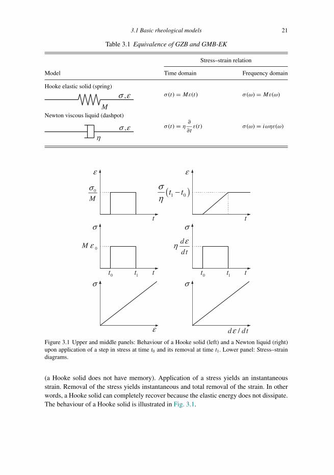
Table 3.1 Equivalence of GZB and GMB-EK
Stress–strain relation
Model Time domain Frequency domain
Hooke elastic solid (spring)
M
,σ ε σ (t) = Mε(t) σ (ω) = Mε(ω)
Newton viscous liquid (dashpot)
,σ εη
σ (t) = η ∂∂tε(t) σ (ω) = iωηε(ω)
ε
0
M
σ
0M ε
( )1 0t tση
−
d
dt
εη
/d dtε
σ
t
ε
σ
σ σ0t 1t t
t
0t 1t t
ε
Figure 3.1 Upper and middle panels: Behaviour of a Hooke solid (left) and a Newton liquid (right)upon application of a step in stress at time t0 and its removal at time t1. Lower panel: Stress–straindiagrams.
(a Hooke solid does not have memory). Application of a stress yields an instantaneousstrain. Removal of the stress yields instantaneous and total removal of the strain. In otherwords, a Hooke solid can completely recover because the elastic energy does not dissipate.The behaviour of a Hooke solid is illustrated in Fig. 3.1.

Trim: 247mm × 174mm Top: 14.762mm Gutter: 23.198mmCUUK2497-03 CUUK2497/Moczo ISBN: 978 1 107 02881 4 November 14, 2013 19:53
22 Rheological models of a continuum
,σ εYσ
Figure 3.2 Saint-Venant body.
3.1.2 Newton viscous liquid
The Newton viscous liquid (N) is a mechanical model for the behaviour of a linearlyviscous liquid in which stress is a linear function of the strain rate. It is represented by adashpot consisting of a cylinder filled with a viscous liquid, and a piston with holes throughwhich the liquid can flow. The only material parameter is a time-independent (Newtonian)viscosity η [Pa s]. The stress–strain relations are given in Table 3.1. Upon application of astep in stress, strain starts linearly to increase. The accumulated strain completely remainsafter removal of the stress (a Newton liquid has extreme memory). We can also say thatthe dashpot is not capable of recovering because all the elastic energy has dissipated. Thebehaviour of a Newton viscous liquid is illustrated in Fig. 3.1.
3.1.3 Saint-Venant plastic solid
Whereas at small strain and stress below some critical value a real material exhibits, ingeneral, linear viscoelastic behaviour, it fails if the stress reaches a critical value – a yieldstress. Failure of a material can result in discontinuous deformation, fracture, or continuousdeformation, plastic flow. In the case of plastic flow, with increasing strain the stress canincrease (so-called strain hardening), decrease (strain softening) or remain constant (idealor pure plasticity). We consider here the third case.
The Saint-Venant body (StV) is a mechanical model for the behaviour of an ideal orpure plastic material. It is represented by a block on a rough base (Fig. 3.2). Note that,in general, the static friction between a block and a base defines a yield stress σ Y. Whenthe applied stress reaches the value of the static friction, the block starts sliding and in ashort time the frictional stress decreases to a smaller value corresponding to a dynamicfriction. In the definition of a Saint-Venant body the static and dynamic friction levelsare not distinguished. Thus, if the applied stress is smaller than the yield stress σ Y, theSaint-Venant body behaves as a rigid solid. If the block starts sliding and the loading stressdoes not decrease below σ Y, the strain increases (at a constant σ = σ Y) to a value thatdepends only on the time duration of the stress application. If the loading stress decreasesbelow σ Y, the sliding stops and the accumulated strain remains.
Clearly, a Saint-Venant body alone can approximate plastic behaviour but it cannotapproximate behaviour before the loading stress reaches σ Y and after (the plastic episode)the stress decreases below σ Y.
Considering the configuration in Fig. 3.2, we can distinguish two possible directions ofstress application and the consequent sliding – to the right and to the left. Choosing, say,the x -axis and stress positive to the right, we can distinguish two values of the yield stress:σ Y and −σ Y. We will come back to the plastic behaviour in Section 3.4.
Trim: 247mm × 174mm Top: 14.762mm Gutter: 23.198mmCUUK2497-03 CUUK2497/Moczo ISBN: 978 1 107 02881 4 November 14, 2013 19:53
3.2 Combined rheological models 23
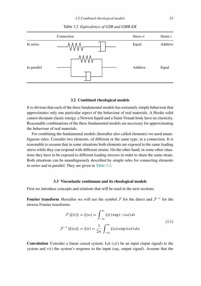
Table 3.2 Equivalence of GZB and GMB-EK
Connection Stress σ Strain ε
In series Equal Additive
In parallel Additive Equal
3.2 Combined rheological models
It is obvious that each of the three fundamental models has extremely simple behaviour thatapproximates only one particular aspect of the behaviour of real materials. A Hooke solidcannot dissipate elastic energy, a Newton liquid and a Saint-Venant body have no elasticity.Reasonable combinations of the three fundamental models are necessary for approximatingthe behaviour of real materials.
For combining the fundamental models (hereafter also called elements) we need unam-biguous rules. Consider two elements, of different or the same type, in a connection. It isreasonable to assume that in some situations both elements are exposed to the same loadingstress while they can respond with different strains. On the other hand, in some other situa-tions they have to be exposed to different loading stresses in order to share the same strain.Both situations can be unambiguously described by simple rules for connecting elementsin series and in parallel. They are given in Table 3.2.
3.3 Viscoelastic continuum and its rheological models
First we introduce concepts and relations that will be used in the next sections.
Fourier transform Hereafter we will use the symbol F for the direct and F−1 for theinverse Fourier transforms:
F {ξ (t)} = ξ (ω) =∫ ∞
−∞ξ (t) exp (−iωt) dt
(3.1)
F−1 {ξ (ω)} = ξ (t) = 1
2π
∫ ∞
−∞ξ (ω) exp (iωt) dω
Convolution Consider a linear causal system. Let iS(t) be an input (input signal) to thesystem and r(t) the system’s response to the input (say, output signal). Assume that the
Trim: 247mm × 174mm Top: 14.762mm Gutter: 23.198mmCUUK2497-03 CUUK2497/Moczo ISBN: 978 1 107 02881 4 November 14, 2013 19:53
24 Rheological models of a continuum
system is invariable with respect to time: if input iS(t) yields response r(t), then inputiS (t − τ ) yields r (t − τ ). Then,
r(t) =∫ t
−∞H (t − τ ) iS(τ )dτ (3.2)
where H(t) is the impulse response of the system, that is, the response of the system to theDirac delta function δ(t) as an input. H(t) characterizes transfer properties of the system inthe time domain. In other words, response r(t) is given by convolution of input iS(t) andimpulse response H(t). Application of the Fourier transform to Eq. (3.2) gives
r(ω) = H(ω)iS(ω) (3.3)
where H(ω) = F {H(t)} is the transfer function in the frequency domain.The integral in Eq. (3.2) is called a convolutory integral. It is obvious that the response at
time t depends on the entire signal iS(t), or, in other words, on the entire history of quantityiS . Therefore, the integral in Eq. (3.2) is also called a hereditary integral.
3.3.1 Stress–strain and strain–stress relations in a viscoelastic continuum
3.3.1.1 Preliminary considerations
A Hooke solid, described by the stress–strain relation (Table 3.1)
σ (t) = Mε(t) (3.4)
has elasticity but no memory and, consequently, is incapable of dissipating energy. We canformally ‘add memory’ by generalizing the simple relation (3.4) to the convolutory relation
σ (t) =∫ t
−∞M (t − τ ) ε(τ )dτ (3.5)
Note that the time-dependent modulus M(t) does not contradict the model invariability withrespect to time – as assumed in the previous section. M(t) behaves in the same way nomatter when the Dirac delta function δ(t) in strain is applied. Application of the Fouriertransform gives
σ (ω) = M(ω)ε(ω) (3.6)
with
σ (ω) = F {σ (t)} , M(ω) = F {M(t)} , ε(ω) = F {ε(t)} (3.7)
We can see that the assumption of a complex and frequency-dependent modulus, andthus assumption of relation (3.6), would be exactly the most natural generalization of thestress–strain relation of a Hooke solid in the frequency domain (Table 3.1).
We can further consider some function ψ(t) being a derivative of M(t):
∂
∂tψ(t) = M(t) (3.8)
Then, due to a property of convolution, Eq. (3.5) can be written as
σ (t) =∫ t
−∞
∂
∂tψ (t − τ ) ε(τ )dτ =
∫ t
−∞ψ (t − τ )
∂
∂τε(τ )dτ (3.9)

Trim: 247mm × 174mm Top: 14.762mm Gutter: 23.198mmCUUK2497-03 CUUK2497/Moczo ISBN: 978 1 107 02881 4 November 14, 2013 19:53
3.3 Viscoelastic continuum and its rheological models 25
Comparing Eq. (3.9) with the relation in Table 3.1 for a Newton liquid we can see thatformally the generalization of perfect elasticity, Eq. (3.5), can be also viewed as a general-ization of pure viscosity.
3.3.1.2 General theory in 1D
For a linear isotropic viscoelastic medium the stress–strain relation can be expressed byEq. (3.9), which can be considered a form of Boltzmann’s superposition and causalityprinciple. Functionψ(t) is the stress relaxation function. With reference to Eq. (3.2),ψ(t) isa stress response to a Dirac delta function in the strain rate or, equivalently, to a Heavisideunit step in the strain. Stress relaxation means a decrease of stress. Considering Eq. (3.5)or (3.8), M(t) is the stress response to a Dirac delta function in strain. Application of theFourier transform to Eq. (3.8) yields
F{∂
∂tψ(t)
}= M(ω) and ψ(ω) = M(ω)
iω(3.10)
and application of the inverse Fourier transform to the latter equation gives
ψ(t) = F−1
{M(ω)
iω
}(3.11)
M(ω) is, in general, a complex frequency-dependent viscoelastic modulus, and Eq. (3.11)is an important relation between the relaxation function and viscoelastic modulus.
Because ψ(t) is the stress response to a Heaviside unit step in strain, we can consider
ψ(t) = ψ(t)H (t); H (t) = 0; t < 0, H (t) = 1; t ≥ 0 (3.12)
Here and hereafter in this chapter, the Heaviside function, H(t), is equal to 1 for zeroargument. Equivalently, ψ(t) = ψ(t); t ≥ 0. Then,
∂ψ
∂t= ∂ψ
∂tH (t) + ψ(t)δ(t) (3.13)
and, according to the first of Eqs. (3.10),
M(ω) =∫ ∞
−∞
[∂ψ
∂tH (t) + ψ(t)δ(t)
]exp(−iωt)dt
= ψ(0) +∫ ∞
0
∂ψ
∂texp(−iωt)dt
= ψ(0) +∫ ∞
0
∂
∂t[ψ(t) − ψ(∞)] exp(−iωt)dt
= ψ(0) + {[ψ(t) − ψ(∞)] exp(−iωt)}|∞0 −∫ ∞
0[ψ(t) − ψ(∞)]
d
dtexp(−iωt)dt
= ψ(0) − [ψ(0) − ψ(∞)] −∫ ∞
0[ψ(t) − ψ(∞)]
d
dtexp(−iωt)dt
= ψ(∞) + iω∫ ∞
0[ψ(t) − ψ(∞)] exp(−iωt)dt
(3.14)

Trim: 247mm × 174mm Top: 14.762mm Gutter: 23.198mmCUUK2497-03 CUUK2497/Moczo ISBN: 978 1 107 02881 4 November 14, 2013 19:53
26 Rheological models of a continuum
Thus,
M(ω) = ψ(∞) + iω∫ ∞
0[ψ(t) − ψ(∞)] exp(−iωt)dt (3.15)
and, consequently,
M(ω = 0) = ψ(t → ∞) (3.16)
Alternatively to Eq. (3.14) we can consider
M(ω) =∫ ∞
−∞
[∂ψ
∂tH (t) + ψ(t)δ(t)
]exp(−iωt)dt
= ψ(0) +∫ ∞
0
∂ψ
∂texp(−iωt)dt
= ψ(0) +[∂ψ
∂t
exp(−iωt)−iω
]∞
0
−∫ ∞
0
∂2ψ
∂t2exp(−iωt)
−iω dt (3.17)
Then,
limω→∞M(ω) = ψ(0) + lim
ω→∞
{[∂ψ
∂t
exp(−iωt)−iω
]∞
0
−∫ ∞
0
∂2ψ
∂t2exp(−iωt)
−iω dt
}= ψ(0) (3.18)
and
M(ω → ∞) = ψ(t = 0) (3.19)
Recall that ψ(t) is a stress response to a Heaviside unit step in strain. Relation (3.19)means that an instantaneous stress response to a Heaviside unit step in strain is equal toM(ω → ∞). Relation (3.16) means that the stress eventually relaxes to a value equal toM(ω = 0). Therefore, it is reasonable to introduce the unrelaxed modulus MU:
MU = limt→0ψ(t) = lim
ω→∞M(ω) (3.20)
relaxed modulus MR:
MR = limt→∞ψ(t) = lim
ω→0M(ω) (3.21)
and modulus defect or relaxation of modulus δM:
δM = MU −MR (3.22)
Alternatively to the stress–strain relation (3.9), it is possible to characterize the behaviourof a viscoelastic medium using the strain–stress relation:
ε(t) =∫ t
−∞χ (t − τ )
∂
∂τσ (τ )dτ (3.23)
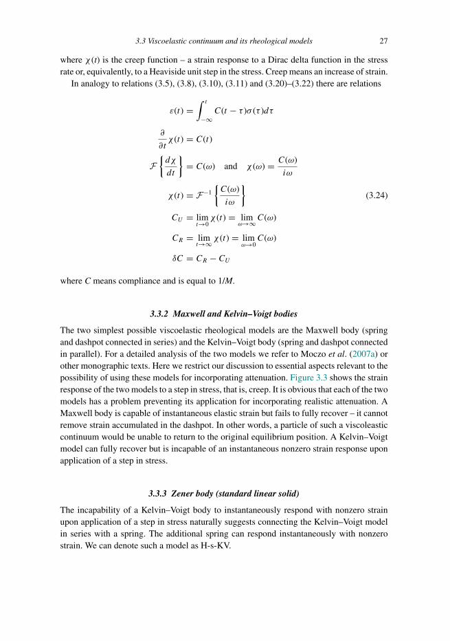
Trim: 247mm × 174mm Top: 14.762mm Gutter: 23.198mmCUUK2497-03 CUUK2497/Moczo ISBN: 978 1 107 02881 4 November 14, 2013 19:53
3.3 Viscoelastic continuum and its rheological models 27
where χ (t) is the creep function – a strain response to a Dirac delta function in the stressrate or, equivalently, to a Heaviside unit step in the stress. Creep means an increase of strain.
In analogy to relations (3.5), (3.8), (3.10), (3.11) and (3.20)–(3.22) there are relations
ε(t) =∫ t
−∞C(t − τ )σ (τ )dτ
∂
∂tχ (t) = C(t)
F{dχ
dt
}= C(ω) and χ (ω) = C(ω)
iω
χ (t) = F−1
{C(ω)
iω
}(3.24)
CU = limt→0χ (t) = lim
ω→∞C(ω)
CR = limt→∞χ (t) = lim
ω→0C(ω)
δC = CR − CU
where C means compliance and is equal to 1/M.
3.3.2 Maxwell and Kelvin–Voigt bodies
The two simplest possible viscoelastic rheological models are the Maxwell body (springand dashpot connected in series) and the Kelvin–Voigt body (spring and dashpot connectedin parallel). For a detailed analysis of the two models we refer to Moczo et al. (2007a) orother monographic texts. Here we restrict our discussion to essential aspects relevant to thepossibility of using these models for incorporating attenuation. Figure 3.3 shows the strainresponse of the two models to a step in stress, that is, creep. It is obvious that each of the twomodels has a problem preventing its application for incorporating realistic attenuation. AMaxwell body is capable of instantaneous elastic strain but fails to fully recover – it cannotremove strain accumulated in the dashpot. In other words, a particle of such a viscoleasticcontinuum would be unable to return to the original equilibrium position. A Kelvin–Voigtmodel can fully recover but is incapable of an instantaneous nonzero strain response uponapplication of a step in stress.
3.3.3 Zener body (standard linear solid)
The incapability of a Kelvin–Voigt body to instantaneously respond with nonzero strainupon application of a step in stress naturally suggests connecting the Kelvin–Voigt modelin series with a spring. The additional spring can respond instantaneously with nonzerostrain. We can denote such a model as H-s-KV.
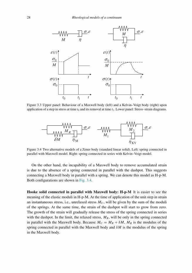
Trim: 247mm × 174mm Top: 14.762mm Gutter: 23.198mmCUUK2497-03 CUUK2497/Moczo ISBN: 978 1 107 02881 4 November 14, 2013 19:53
28 Rheological models of a continuum
M η
,σ εM
η
,σ ε
( )tε
( )tσ
0t 1t 0t 1t tt
tt
0
M
σ
0σ
( )tε
( )tσ0σ
0
M
σ
Figure 3.3 Upper panel: Behaviour of a Maxwell body (left) and a Kelvin–Voigt body (right) uponapplication of a step in stress at time t0 and its removal at time t1. Lower panel: Stress–strain diagrams.
RM
Mδ Mη
,σ ε
1M2M
KVη
,σ ε
Figure 3.4 Two alternative models of a Zener body (standard linear solid). Left: spring connected inparallel with Maxwell model. Right: spring connected in series with Kelvin–Voigt model.
On the other hand, the incapability of a Maxwell body to remove accumulated strainis due to the absence of a spring connected in parallel with the dashpot. This suggestsconnecting a Maxwell body in parallel with a spring. We can denote this model as H-p-M.Both configurations are shown in Fig. 3.4.
Hooke solid connected in parallel with Maxwell body: H-p-M It is easier to see themeaning of the elastic moduli in H-p-M. At the time of application of the unit step in strainan instantaneous stress, i.e., unrelaxed stress MU , will be given by the sum of the moduliof the springs. At the same time, the strain of the dashpot will start to grow from zero.The growth of the strain will gradually release the stress of the spring connected in serieswith the dashpot. In the limit, the relaxed stress,MR , will be only in the spring connectedin parallel with the Maxwell body. Because MU = MR + δM , MR is the modulus of thespring connected in parallel with the Maxwell body and δM is the modulus of the springin the Maxwell body.
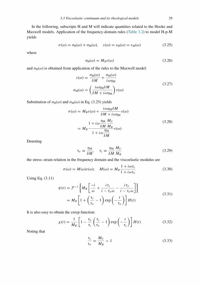
Trim: 247mm × 174mm Top: 14.762mm Gutter: 23.198mmCUUK2497-03 CUUK2497/Moczo ISBN: 978 1 107 02881 4 November 14, 2013 19:53
3.3 Viscoelastic continuum and its rheological models 29
In the following, subscripts H and M will indicate quantities related to the Hooke andMaxwell models. Application of the frequency-domain rules (Table 3.2) to model H-p-Myields
σ (ω) = σH(ω) + σM(ω), ε(ω) = εH(ω) = εM(ω) (3.25)
where
σH(ω) = MRε(ω) (3.26)
and σH(ω) is obtained from application of the rules to the Maxwell model:
ε(ω) = σM(ω)
δM+ σM(ω)
iωηM
σM(ω) =(iωηMδM
δM + iωηM
)ε(ω)
(3.27)
Substitution of σH(ω) and σM(ω) in Eq. (3.25) yields
σ (ω) = MRε(ω) + iωηMδM
δM + iωηMε(ω)
= MR1 + iω ηM
δM
MU
MR
1 + iω ηM
δM
ε(ω)
(3.28)
Denoting
τσ ≡ ηM
δM, τε ≡ ηM
δM
MU
MR(3.29)
the stress–strain relation in the frequency domain and the viscoelastic modulus are
σ (ω) = M(ω)ε(ω); M(ω) = MR 1 + iωτε1 + iωτσ (3.30)
Using Eq. (3.11)
ψ(t) = F−1
{MR
[−iω
+ iτε
i − τσω − iτσ
i − τσω]}
= MR[
1 +(τε
τσ− 1
)exp
(− t
τσ
)]H (t)
(3.31)
It is also easy to obtain the creep function:
χ (t) = 1
MR
[1 − τσ
τε
(τε
τσ− 1
)exp
(− t
τε
)]H (t) (3.32)
Noting that
τε
τσ= MU
MR> 1 (3.33)

Trim: 247mm × 174mm Top: 14.762mm Gutter: 23.198mmCUUK2497-03 CUUK2497/Moczo ISBN: 978 1 107 02881 4 November 14, 2013 19:53
30 Rheological models of a continuum
it is clear from relations (3.31) and (3.32) that τσ and τε have the meanings of characteristicstress-relaxation time and characteristic creep time, respectively.
Hooke solid connected in series with Kelvin–Voigt body: H-s-KV Application of thefrequency-domain rules (Table 3.2) to model H-s-KV yields
σ (ω) = σH(ω) = σKV(ω), ε(ω) = εH(ω) + εKV(ω) (3.34)
where
εH(ω) = σ (ω)
M1(3.35)
Application of the rules to the Kelvin–Voigt model gives
σ (ω) = M2εKV(ω) + iωηKVεKV(ω) (3.36)
Then,
ε(ω) =(
1
M1+ 1
M2 + iωηKV
)σ (ω) (3.37)
σ (ω) = M1M2 + iωηKVM1
M1 +M2 + iωηKVε(ω) (3.38)
and
σ (ω) = M(ω)ε(ω), M(ω) = M1M2
M1 +M2
1 + iωηKV
M2
1 + iω ηKV
M1 +M2
(3.39)
The unrelaxed and relaxed moduli are
limω→∞M(ω) = M1, lim
ω→0M(ω) = M1M2
M1 +M2(3.40)
The relations between moduli M1 and M2 in H-s-KV and moduli MR and δM in H-p-Mare
MR = M1M2
M1 +M2, δM = M2
1
M1 +M2(3.41)
The behaviour of a Zener body is illustrated in Fig. 3.5.Viscosities ηKV and ηM of the H-s-KV and H-p-M, respectively, are related by
ηKV = ηM
(MU
δM
)2
(3.42)
Note that for a given set ofMR , δM and ηM in H-p-M it would be impossible to find moduliM1 andM2 if we assumed ηKV = ηM.
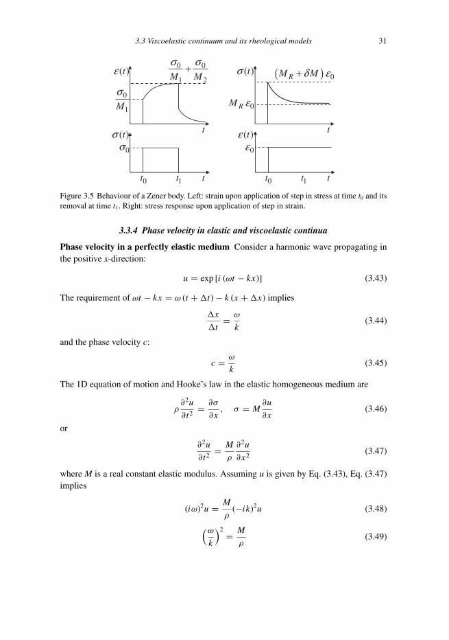
Trim: 247mm × 174mm Top: 14.762mm Gutter: 23.198mmCUUK2497-03 CUUK2497/Moczo ISBN: 978 1 107 02881 4 November 14, 2013 19:53
3.3 Viscoelastic continuum and its rheological models 31
( )tε ( )tσ
( )tσ ( )tε0σ 0ε
0t 1t 0t 1t tt
tt
0RM ε0
1M
σ
0 0
1 2M M
σ σ+ ( ) 0RM Mδ ε+
Figure 3.5 Behaviour of a Zener body. Left: strain upon application of step in stress at time t0 and itsremoval at time t1. Right: stress response upon application of step in strain.
3.3.4 Phase velocity in elastic and viscoelastic continua
Phase velocity in a perfectly elastic medium Consider a harmonic wave propagating inthe positive x-direction:
u = exp [i (ωt − kx)] (3.43)
The requirement of ωt − kx = ω (t +�t) − k (x +�x) implies
�x
�t= ω
k(3.44)
and the phase velocity c:
c = ω
k(3.45)
The 1D equation of motion and Hooke’s law in the elastic homogeneous medium are
ρ∂2u
∂t2= ∂σ
∂x, σ = M∂u
∂x(3.46)
or
∂2u
∂t2= M
ρ
∂2u
∂x2(3.47)
where M is a real constant elastic modulus. Assuming u is given by Eq. (3.43), Eq. (3.47)implies
(iω)2u = M
ρ(−ik)2u (3.48)
(ωk
)2= M
ρ(3.49)
Trim: 247mm × 174mm Top: 14.762mm Gutter: 23.198mmCUUK2497-03 CUUK2497/Moczo ISBN: 978 1 107 02881 4 November 14, 2013 19:53
32 Rheological models of a continuum
The phase velocity is
c = ω
k=(M
ρ
) 12
(3.50)
Phase velocity in a viscoelastic medium The 1D equation of motion and Hooke’s law inthe viscoelastic medium are
ρ∂2u
∂t2= ∂σ
∂x, σ = M(t) ∗ ∂u
∂x(3.51)
or
ρ∂2u
∂t2= M(t) ∗ ∂
2u
∂x2(3.52)
where the asterisk indicates the convolution. Application of the Fourier transform to Eq.(3.52) gives
(iω)2 F {u} = M(ω)
ρ
∂2
∂x2F {u} (3.53)
whereM(ω) is, in general, the complex frequency-dependent viscoelastic modulus. In orderto distinguish the wavenumber in the viscoelastic medium from that in the elastic medium,we denote it by K . Then, for any wave (the harmonic wave being a special case),
u (t, x) = u(t) exp (−iKx) (3.54)
we obtain
∂2
∂x2F {u} = −K2F {u} (3.55)
Equation (3.53) implies
−ω2 = M(ω)
ρ(−K2) (3.56)
and
K
ω=√
ρ
M(ω)(3.57)
Assuming real ω, Eq. (3.57) implies that K may be complex:
K = Kreal + iKimag (3.58)
Generalization of the wave in Eq. (3.43) with the complex wavenumber K gives
u = exp(Kimagx) exp[i(ωt −Krealx)] (3.59)
In analogy with Eqs. (3.43) and (3.45), the real phase velocity is
c = ω
Kreal(3.60)

Trim: 247mm × 174mm Top: 14.762mm Gutter: 23.198mmCUUK2497-03 CUUK2497/Moczo ISBN: 978 1 107 02881 4 November 14, 2013 19:53
3.3 Viscoelastic continuum and its rheological models 33
Considering (3.57) and (3.60) we obtain
1
c= Kreal
ω=(√
ρ
M(ω)
)real
(3.61)
Consequently, we can use the symbol of real k instead of Kreal,
k ≡ Kreal (3.62)
and write
K = k + iKimag (3.63)
We can also define a complex velocity V = Vreal + iVimag as
V ≡√M(ω)
ρ(3.64)
Using Eqs. (3.57), (3.63) and (3.64),
k = ωVreal
|V |2 , Kimag = −ωVimag
|V |2 (3.65)
ConsideringM = Mreal + iMimag we obtain
Mreal
ρ= V 2
real − V 2imag,
Mimag
ρ= 2VrealVimag (3.66)
We easily find the relation between the complex velocity V and the real phase velocity cusing Eqs. (3.61) and (3.65):
c = |V |2Vreal
= V 2real + V 2
imag
Vreal(3.67)
3.3.5 Measure of dissipation and attenuation in a viscoelastic continuum
Whereas a Hooke perfectly elastic solid does not dissipate elastic (or strain) energy at all,a Newton viscous liquid dissipates the energy completely but has no elasticity. A Zenerbody, properly combining a Hooke solid and a Newton liquid, is capable of both an elasticresponse and energy dissipation. A Hooke solid is characterized by a real elastic frequency-independent modulus, a Zener body by a complex frequency-dependent viscoelastic mod-ulus. Therefore, one may intuitively guess that the ratio between the imaginary and realparts of the viscoelastic modulus,Mimag/Mreal, might be related to some measure of dissi-pation. Indeed, O’Connell and Budiansky (1978) suggested using this ratio as a measure ofdissipation in a viscoelastic medium. Correspondingly, they suggested a definition of thequality parameterQ of the medium (a term borrowed from electric circuit theory) as
Q(ω) = Mreal
Mimag(3.68)
Trim: 247mm × 174mm Top: 14.762mm Gutter: 23.198mmCUUK2497-03 CUUK2497/Moczo ISBN: 978 1 107 02881 4 November 14, 2013 19:53
34 Rheological models of a continuum
In seismology, Q is commonly termed a quality factor. O’Connell and Budiansky (1978)showed that Q is related to the energy dissipated per oscillation cycle assuming harmonicloading in a unit volume of the continuum:
1
Q(ω)= 1
4π
Edissipated
Eaverage(3.69)
Here Edissipated is the dissipated energy and Eaverage is the average elastic energy storedduring one cycle of loading.
Note that the ratio of the imaginary and real parts of the viscoelastic modulus was usedas a loss parameter previously by White (1965) in his book on seismic waves.
Anelastic dissipation causes attenuation of free oscillations in time or spatial attenuationof a propagating wave.
Recall wave (3.59) with k used instead of Kreal:
u = exp(Kimagx) exp[i(ωt − kx)] (3.70)
Assume that u has its peak value at xP . Consider a fixed time t and evaluate the ratio of theu values at xP + λ and xP , where λ is the wavelength:
u(xP + λ, t)u(xP , t)
= exp(Kimagλ) exp(−ikλ) = exp(Kimagλ) (3.71)
The latter equality is due to kλ = 2π . It is clear thatKimag has to be negative if the amplitudedecays with distance. Indeed, the attenuation coefficient α > 0 is defined as
α = −Kimag (3.72)
and thus,
u(xP + λ, t)u(xP , t)
= exp (−αλ) (3.73)
The spatialQ is defined by relation
exp(−αλ) = exp
(− π
Qspatial
)(3.74)
Hence,
Qspatial = π
αλ= k
2α(3.75)
Using Eqs. (3.65) and (3.72) we obtain
Qspatial = Vreal
2Vimag(3.76)
CompareQspatial withQ defined by Eq. (3.68). Using Eq. (3.66),
Q = Mreal
Mimag= V 2
real − V 2imag
2VrealVimag= Vreal
2Vimag− Vimag
2Vreal(3.77)

Trim: 247mm × 174mm Top: 14.762mm Gutter: 23.198mmCUUK2497-03 CUUK2497/Moczo ISBN: 978 1 107 02881 4 November 14, 2013 19:53
3.3 Viscoelastic continuum and its rheological models 35
Using Eq. (3.76) we obtain
Q = Qspatial − 1
4Qspatial(3.78)
AssumingQspatial 1 we haveQ ≈ Qspatial. Consider, e.g.,Qspatial = 10. ThenQ = 9.975.ForQspatial = 5 there isQ = 4.95. These are small differences that can be neglected in mostnumerical applications.
For more details we refer to the article by O’Connell and Budiansky (1978) and, forexample, books by Aki and Richards (2002), and Pujol (2003).
3.3.6 Attenuation in a Zener body
The viscoelastic modulus given by Eq. (3.30) can be written as
M(ω) = MR 1 + ω2τσ τε + iω (τε − τσ )
1 + ω2τ 2σ
(3.79)
Equation (3.79) implies
1
Q(ω)= Mimag(ω)
Mreal(ω)= ω (τε − τσ )
1 + ω2τσ τε(3.80)
Q−1(ω) has its maximum at frequency
ωm = 1√τσ τε
= δM
η
√MR
MU(3.81)
Q−1(ω) is illustrated in Fig. 3.6. It is clear from the figure that one Zener body cannotapproximate, for instance, constant or almost constant Q(ω). A superposition of severalZener bodies whose peaks are properly distributed over a desired frequency range mightprovide a reasonable approximation.
3.3.7 Generalized Zener body
A generalized Zener body (GZB) is a parallel connection of n Zener bodies. Consider eachof them to be of the H-p-M type (Fig. 3.7). The relaxed modulus MRl , modulus defectδMl and viscosity ηl characterize each l-th Zener body. We denote by Ml , MUl , τσ l andτεl the viscoelastic modulus, unrelaxed modulus, characteristic stress-relaxation time andcharacteristic creep time of the l-th Zener body, respectively. Denoting stress and strainof the l-th Zener body by σl(ω) and εl(ω), application of the frequency-domain rules forcombined models yields
σ (ω) =∑n
l=1σl(ω), ε(ω) = εl(ω); l = 1, 2, . . . , n (3.82)

Trim: 247mm × 174mm Top: 14.762mm Gutter: 23.198mmCUUK2497-03 CUUK2497/Moczo ISBN: 978 1 107 02881 4 November 14, 2013 19:53
36 Rheological models of a continuum
0.02 0.2 2 20 200 0.000
0.002
0.004
0.006
0.008
0.010
0.012
1( )Q ω−
0.02 0.2 2 20 200 ωπ π π π π
0.012
0.010
0.008
0.006
0.004
0.002
0.000
Figure 3.6 Q−1(ω) of Zener body.
Using Eq. (3.30),
σl(ω) = Ml(ω)ε(ω); Ml(ω) = MRl 1 + iωτεl1 + iωτσl (3.83)
with
τσ l ≡ ηl
δMl, τεl ≡ ηl
δMl
MUl
MRl(3.84)
we obtain
σ (ω) = M(ω)ε(ω), M(ω) =∑n
l=1MRl
1 + iωτεl1 + iωτσl (3.85)
The relaxed and unrelaxed moduli are
MR = limω→0
M(ω) =∑n
l=1MRl (3.86)
and, using Eq. (3.33),
MU = limω→∞M(ω) =
∑n
l=1MRl
τεl
τσ l=∑n
l=1MUl
=∑n
l=1(MRl + δMl) = MR + δM (3.87)
where δM is the modulus defect (relaxation of modulus):
δM =∑n
l=1δMl (3.88)
As expected, upon application of a unit step in strain, the instantaneous elastic response,quantified by the unrelaxed modulus MU , is due to the superposition of all the springs in
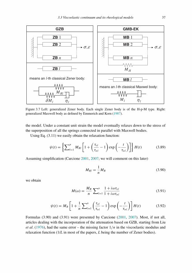
Trim: 247mm × 174mm Top: 14.762mm Gutter: 23.198mmCUUK2497-03 CUUK2497/Moczo ISBN: 978 1 107 02881 4 November 14, 2013 19:53
3.3 Viscoelastic continuum and its rheological models 37
RlM
lMδ lη lM lη
GZB GMB-EK
ZB 1
ZB 2
ZB n
ZB l
means an l-th classical Zener body:
MB 1
MB 2
MB n
MB l
means an l-th classical Maxwel body:
HM
,σ ε ,σ ε
Figure 3.7 Left: generalized Zener body. Each single Zener body is of the H-p-M type. Right:generalized Maxwell body as defined by Emmerich and Korn (1987).
the model. Under a constant unit strain the model eventually relaxes down to the stress ofthe superposition of all the springs connected in parallel with Maxwell bodies.
Using Eq. (3.11) we easily obtain the relaxation function:
ψ(t) ={∑n
l=1MRl
[1 +
(τεl
τσ l− 1
)exp
(− t
τσ l
)]}H (t) (3.89)
Assuming simplification (Carcione 2001, 2007; we will comment on this later)
MRl = 1
nMR (3.90)
we obtain
M(ω) = MR
n
∑n
l=1
1 + iωτεl1 + iωτσl (3.91)
ψ(t) = MR[
1 + 1
n
∑n
l=1
(τεl
τσ l− 1
)exp
(− t
τσ l
)]H (t) (3.92)
Formulas (3.90) and (3.91) were presented by Carcione (2001, 2007). Most, if not all,articles dealing with the incorporation of the attenuation based on GZB, starting from Liuet al. (1976), had the same error – the missing factor 1/n in the viscoelastic modulus andrelaxation function (1/L in most of the papers, L being the number of Zener bodies).

Trim: 247mm × 174mm Top: 14.762mm Gutter: 23.198mmCUUK2497-03 CUUK2497/Moczo ISBN: 978 1 107 02881 4 November 14, 2013 19:53
38 Rheological models of a continuum
The attenuation corresponding toM(ω) given by Eq. (3.85) is quantified by
1
Q(ω)= Mimag(ω)
Mreal(ω)=
∑nl=1MRl
ω (τεl − τσ l)1 + ω2τ 2
σ l∑nl=1MRl
1 + ω2τεlτσ l
1 + ω2τ 2σ l
(3.93)
from which a simplified version due to (3.90) is obtained immediately.Before we quantitatively illustrate the attenuation in the GZB model we look at an
alternative model published by Emmerich and Korn (1987).
3.3.8 Generalized Maxwell body
The model published by Emmerich and Korn (1987) is shown in Fig. 3.7. Note that oftenin the literature on rheology the generalized Maxwell body is defined as nMaxwell bodiesconnected in parallel, that is, without the additional spring. The additional spring here,however, makes that significant difference. Therefore, we use the abbreviation GMB-EKinstead of just GMB.
The l-th Maxwell body is characterized by elastic modulus Ml and viscosity ηl . Theadditional Hooke spring is characterized by elastic modulus MH. Subscript l will indicatethe l-th Maxwell body whereas subscript H will indicate the additional spring. Applicationof the rules in the frequency domain yields
σ (ω) = σH(ω) +∑n
l=1σl(ω), ε(ω) = εH(ω) = εl(ω); l = 1, 2, . . . , n (3.94)
where
σH(ω) = MHε(ω) (3.95)
ε(ω) = εl(ω) = σl(ω)
Ml+ σl(ω)
iωηl(3.96)
The latter equation implies
σl(ω) = iηlMlω
Ml + iηlω ε(ω) (3.97)
Define a characteristic frequency
ωl ≡ Ml
ηl(3.98)
Then,
σ (ω) = M(ω)ε(ω), M(ω) = MH +∑n
l=1
iMlω
ωl + iω (3.99)

Trim: 247mm × 174mm Top: 14.762mm Gutter: 23.198mmCUUK2497-03 CUUK2497/Moczo ISBN: 978 1 107 02881 4 November 14, 2013 19:53
3.3 Viscoelastic continuum and its rheological models 39
The relaxed and unrelaxed moduli are
MU = limω→∞M(ω) = MH +
∑n
l=1Ml
(3.100)MR = lim
ω→0M(ω) = MH
BecauseMU = MR + δM ,
δM =∑n
l=1Ml (3.101)
and Ml has the meaning of δMl . As expected, upon application of a unit step in strain,the instantaneous elastic response, quantified by the unrelaxed modulus MU , is due tosuperposition of all springs in the model. Under a constant unit strain the model eventuallyrelaxes down to the stress of the additional spring, that is, MH. Compare this with theanalogous statement regarding the GZB model after Eq. (3.87): the additional spring inthe GMB model plays the same role as all the springs connected in parallel with Maxwellbodies in individual Zener bodies together.
Using Eq. (3.11), the second of Eqs. (3.99) and Eq. (3.100) we obtain the relaxationfunction
ψ(t) =[MR +
n∑l=1
Mle−ωl t
]H (t) (3.102)
The viscoelastic modulus and relaxation function can also be expressed using the unrelaxedmodulus. In the second of Eqs. (3.99) we replace MH by difference MU − δM , then δMusing Eq. (3.101), and obtain
M(ω) = MU −∑n
l=1
Mlωl
ωl + iω (3.103)
Similarly we modify Eq. (3.102):
ψ(t) =[MU −
∑n
l=1Ml(1 − e−ωl t)]H (t) (3.104)
The attenuation corresponding toM(ω) given by Eq. (3.103) is quantified by
1
Q(ω)= Mimag(ω)
Mreal(ω)=
∑nl=1
Mlωlω
ω2l + ω2
MU −∑nl=1
Mlω2l
ω2l + ω2
(3.105)
Before we continue with the attenuation we compare the GZB and GMB-EK models.
3.3.9 Equivalence of GZB and GMB-EK
The viscoelastic modulus of GZB is usually presented in the literature in the form ofEq. (3.85), or in the simplified form of Eq. (3.91). Consider, however, expressions for the
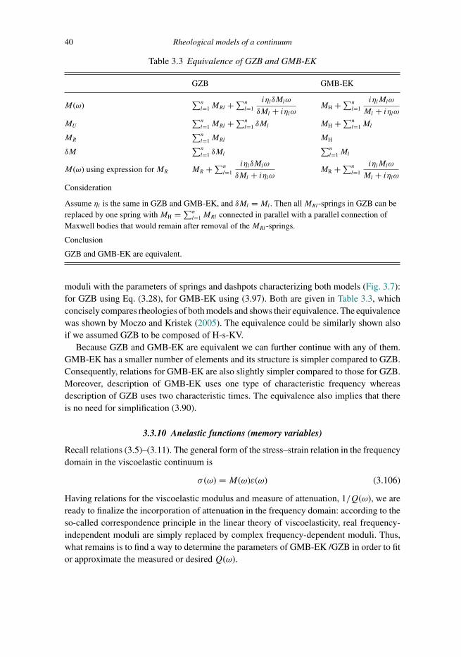
Trim: 247mm × 174mm Top: 14.762mm Gutter: 23.198mmCUUK2497-03 CUUK2497/Moczo ISBN: 978 1 107 02881 4 November 14, 2013 19:53
40 Rheological models of a continuum
Table 3.3 Equivalence of GZB and GMB-EK
GZB GMB-EK
M(ω)∑nl=1MRl +
∑nl=1
iηlδMlω
δMl + iηlω MH +∑nl=1
iηlMlω
Ml + iηlωMU
∑nl=1MRl +
∑nl=1 δMl MH +∑n
l=1Ml
MR
∑nl=1MRl MH
δM∑nl=1 δMl
∑nl=1Ml
M(ω) using expression forMR MR +∑nl=1
iηlδMlω
δMl + iηlω MR +∑nl=1
iηlMlω
Ml + iηlωConsideration
Assume ηl is the same in GZB and GMB-EK, and δMl = Ml . Then allMRl-springs in GZB can bereplaced by one spring withMH = ∑n
l=1MRl connected in parallel with a parallel connection ofMaxwell bodies that would remain after removal of theMRl-springs.
Conclusion
GZB and GMB-EK are equivalent.
moduli with the parameters of springs and dashpots characterizing both models (Fig. 3.7):for GZB using Eq. (3.28), for GMB-EK using (3.97). Both are given in Table 3.3, whichconcisely compares rheologies of both models and shows their equivalence. The equivalencewas shown by Moczo and Kristek (2005). The equivalence could be similarly shown alsoif we assumed GZB to be composed of H-s-KV.
Because GZB and GMB-EK are equivalent we can further continue with any of them.GMB-EK has a smaller number of elements and its structure is simpler compared to GZB.Consequently, relations for GMB-EK are also slightly simpler compared to those for GZB.Moreover, description of GMB-EK uses one type of characteristic frequency whereasdescription of GZB uses two characteristic times. The equivalence also implies that thereis no need for simplification (3.90).
3.3.10 Anelastic functions (memory variables)
Recall relations (3.5)–(3.11). The general form of the stress–strain relation in the frequencydomain in the viscoelastic continuum is
σ (ω) = M(ω)ε(ω) (3.106)
Having relations for the viscoelastic modulus and measure of attenuation, 1/Q(ω), we areready to finalize the incorporation of attenuation in the frequency domain: according to theso-called correspondence principle in the linear theory of viscoelasticity, real frequency-independent moduli are simply replaced by complex frequency-dependent moduli. Thus,what remains is to find a way to determine the parameters of GMB-EK /GZB in order to fitor approximate the measured or desiredQ(ω).

Trim: 247mm × 174mm Top: 14.762mm Gutter: 23.198mmCUUK2497-03 CUUK2497/Moczo ISBN: 978 1 107 02881 4 November 14, 2013 19:53
3.3 Viscoelastic continuum and its rheological models 41
However, aiming to incorporate realistic attenuation in the time domain, we have torecall the stress–strain relation in the time domain:
σ (t) =∫ t
−∞M(t − τ )ε(τ )dτ (3.107)
with
M(t) = F−1 {M(ω)} or M(t) = ∂
∂tψ(t) (3.108)
Although we are ready to determine M(t), we still have a problem: with relation (3.107)we need the entire history of strain in order to determine stress at time t at each spatialposition. Moreover, we have to evaluate the convolutory integral at each time. This is, inpractice, intractable or at least very inefficient – anticipating, for instance, no fewer than106–108 spatial grid points and 103–104 time levels to be calculated in the grid methods.A reasonable solution of the problem is to introduce anelastic functions (also memoryvariables, new variables or internal variables).
Recall the relaxation function for GMB-EK, Eq. (3.104):
ψ(t) =[MU −
∑n
l=1Ml(1 − e−ωl t)]H (t) (3.109)
Then,
M(t) = −∑n
l=1Mlωle
−ωl tH (t) +[MU −
∑n
l=1Ml(1 − e−ωl t)] δ(t) (3.110)
Substituting the r.h.s. forM(t) in Eq. (3.107) yields
σ (t) = −∫ t
−∞
∑n
l=1Mlωle
−ωl (t−τ )H (t − τ )ε(τ )dτ
+∫ t
−∞MUδ(t − τ )ε(τ )dτ
−∫ t
−∞
∑n
l=1Ml[1 − e−ωl (t−τ )]δ(t − τ )ε(τ )dτ (3.111)
and
σ (t) = MUε(t) −∑n
l=1Mlωl
∫ t
−∞e−ωl (t−τ )ε(τ )dτ (3.112)
Now it is possible to replace the convolution integral by anelastic functions. Whereas Dayand Minster (1984), Emmerich and Korn (1987) and Carcione et al. (1988a,b) defined theanelastic functions (additional internal variables, memory variables) as dependent also onthe material properties, for an important reason that will be explained later, Kristek andMoczo (2003) defined their anelastic functions as independent of the material properties.Here we follow Kristek and Moczo (2003). Defining anelastic functions
ζl(t) = ωl∫ t
−∞e−ωl (t−τ )ε(τ )dτ , l = 1, . . . , n (3.113)

Trim: 247mm × 174mm Top: 14.762mm Gutter: 23.198mmCUUK2497-03 CUUK2497/Moczo ISBN: 978 1 107 02881 4 November 14, 2013 19:53
42 Rheological models of a continuum
we rewrite the latter stress–strain relation as
σ (t) = MUε(t) −∑n
l=1Mlζl(t) (3.114)
The stress–strain relation is now simple to evaluate if we know the anelastic functions.Differentiate Eq. (3.113) with respect to time:
∂
∂tζl(t) = ωl
[−ωl
∫ t
−∞e−ωl (t−τ )ε(τ )dτ + ε(t)
](3.115)
The first term in the brackets is equal to −ζl(t) and consequently
∂
∂tζl(t) + ωlζl(t) = ωlε(t), l = 1, . . . , n (3.116)
Equations (3.114) and (3.116) together represent the time-domain stress–strain relationsfor the viscoelastic continuum with GMB-EK/GZB rheology. The need to know the entirehistory of strain at each spatial position and evaluate the convolutory integral at each timeis replaced by using additional functional variables that can be obtained by solving theadditional differential equations (3.116).
Having the relation for stress is sufficient for the displacement–stress formulation andfor developing the displacement formulation. We should also consider the velocity–stressformulation.
Temporal differentiation of Eqs. (3.114) and (3.116) gives
∂
∂tσ (t) = MU ∂
∂tε(t) −
∑n
l=1Mlξl(t) (3.117)
∂
∂tξl(t) + ωlξl(t) = ωl ∂
∂tε(t), l = 1, . . . , n (3.118)
with
ξl(t) = ∂
∂tζl(t), l = 1, . . . , n (3.119)
Equations (3.112), (3.114) and (3.117) clearly decompose the whole stress into elasticand anelastic parts. The elastic part is proportional to the unrelaxed modulus MU thatcorresponds to the elastic modulus in a perfectly elastic continuum. The anelastic partis determined by moduli Ml and anelastic functions ζl(t). We need to know how to findparameters of GMB-EK/GZB in order to fit or approximate the measured or desiredQ(ω).
As mentioned in the introduction to this chapter, for many years two parallel sets ofpublications and algorithms were developed for the GMB-EK or GZB models. We showhere equations equivalent to those presented by Robertsson et al. (1994) for GZB. UsingEqs. (3.89), (3.8), (3.5), (3.86) and (3.87) we can obtain the stress–strain relation
∂
∂tσ (t) = MU ∂
∂tε(t) −
∑n
l=1rl(t) (3.120)
Trim: 247mm × 174mm Top: 14.762mm Gutter: 23.198mmCUUK2497-03 CUUK2497/Moczo ISBN: 978 1 107 02881 4 November 14, 2013 19:53
3.3 Viscoelastic continuum and its rheological models 43
and relaxation functions
rl(t) = MRl
τσ l
(1 − τεl
τσ l
)∫ t
−∞
∂
∂tε(τ ) exp
[−(t − τ )/τσ l]dτ, l = 1, . . . , n (3.121)
rl(t) + 1
τσ lrl(t) = MRl
τσ l
(1 − τεl
τσ l
)∂
∂tε(t), l = 1, . . . , n (3.122)
3.3.11 Anelastic coefficients and unrelaxed modulus
We can define anelastic coefficients
Yl = Ml
MU; l = 1, . . . , n (3.123)
(Do not mix these up with the lower-case yl = Ml/MR; l = 1, . . . , n, used by Emmerich
and Korn, 1987.) The stress–strain relations (3.114) and (3.117) become
σ (t) = MU[ε(t) −
∑n
l=1Ylζl(t)
](3.124)
∂
∂tσ (t) = MU
[∂
∂tε(t) −
∑n
l=1Ylξl(t)
](3.125)
and Eqs. (3.116) and (3.118) remain unchanged. The viscoelastic and relaxed moduli are
M(ω) = MU[
1 −∑n
l=1Yl
ωl
ωl + iω]
(3.126)
MR = MU(
1 −∑n
l=1Yl
)(3.127)
Note thatMU∑nl=1 Yl represents the modulus defect (or relaxation of modulus).
The attenuation corresponding toM(ω) given by Eq. (3.126) is quantified by
1
Q(ω)= Mimag(ω)
Mreal(ω)=
∑nl=1 Yl
ωlω
ω2l + ω2
1 −∑nl=1 Yl
ω2l
ω2l + ω2
(3.128)
The equation can be rewritten as
Q−1(ω) =∑n
l=1
ωlω + ω2l Q
−1(ω)
ω2l + ω2
Yl (3.129)
Assume that values ofQ(ω) in a frequency range of interest are known – they are measuredor estimated. We can choose the number and values of the characteristic frequencies ωl inorder to reasonably cover the frequency range of interest. (Frequencies ωl are the same forthe whole computational domain.) Considering,for instance,Q values at frequencies ωk , asystem of equations (3.129), one equation for eachQ (ωk), is obtained. The system can be

Trim: 247mm × 174mm Top: 14.762mm Gutter: 23.198mmCUUK2497-03 CUUK2497/Moczo ISBN: 978 1 107 02881 4 November 14, 2013 19:53
44 Rheological models of a continuum
solved for the anelastic coefficients Yl using the least-square method. The application of theleast-square method leads to a system of n equations for n unknown anelastic coefficients.
Emmerich and Korn (1987) demonstrated that a sufficiently accurate approximation tonearly constant Q(ω) is obtained if frequencies ωl cover the frequency range of interestlogarithmically equidistantly. One possibility is to considerQ values at 2n− 1 frequenciesωk , andω1 = ω1,ω2 = ω3, . . . ,ωn = ω2n−1. Emmerich and Korn (1987) showed that n = 3is sufficient for the frequency range [ωmin, 100ωmin]. A simple possible choice is ω1 = ωmin.A more detailed discussion of the frequency range and its sampling by frequencies ωk canbe found in the article by Graves and Day (2003; Eqs. 13 and 14). For an efficient andaccurate determination of the parameters of the GMB-EK see Liu and Archuleta (2006).
If the phase velocity at a certain reference frequency ωref , that is c(ωref
), is known from
measurements, the unrelaxed modulus MU can be determined from the value of c(ωref
)and the viscoelastic modulus. Recall that
1
c(ω)= Re
{(M(ω)
ρ
)−1/2}
(3.130)
From Eqs. (3.126) and (3.130) we obtain (Moczo et al. 1997)
MU = ρc2(ωref
) R +�1
2R2(3.131)
where
R = (�2
1 +�22
)1/2,
�1 = 1 −∑n
l=1Yl
ω2l
ω2l + ω2
ref
, �2 =∑n
l=1Ylωlωref
ω2l + ω2
ref
(3.132)
If we knowQ(ω) and c(ωref
)from measurements, and if we assume viscoelastic rheology
of GMB-EK/GZB, we can determine the parameters of the viscoelastic stress–strain relationusing Eqs. (3.129) and (3.131) for a chosen set of frequencies ωl reasonably covering thefrequency range of interest.
3.3.12 Attenuation and phase velocity in GMB-EK/GZB continuum
In Fig. 3.8 we illustrate the attenuation and phase velocity for S waves, Q−1(ω) and c(ω),obtained using the GMB-EK/GZB rheology assuming the exact constant Q(ω) = 20 andthe exact phase velocity c(ωref ) = 200 m/s specified at the reference frequencyωref = 2π1.Three relaxation frequencies are assumed: ω1 = 2π0.04, ω2 = 2π0.4, ω3 = 2π4 in orderto sufficiently accurately approximate the attenuation in the frequency range [0.04, 4] Hz.This approximation was used in the modelling of seismic motion in the sedimentaryMygdonian basin near Thessaloniki, Greece, in the E2VP (EuroSeistest Verification andValidation Project; see also Chapter 19).

Trim: 247mm × 174mm Top: 14.762mm Gutter: 23.198mmCUUK2497-03 CUUK2497/Moczo ISBN: 978 1 107 02881 4 November 14, 2013 19:53
3.3 Viscoelastic continuum and its rheological models 45
0.1 1 10 100
0.01
0.02
0.03
0.04
0.05
0.06
0.07
0.1 1 6.310 100
185
190
195
200
205
210
215
0.1 1 10 100
0.070.060.050.040.030.020.01
215210205200195190185
0.1 1 10 100
2π
1Q− c
ω ωFigure 3.8 Left: Q−1(ω) exact (dashed) and approximated (solid). The approximation is obtained forthree relaxation frequencies ω1 = 2π0.04, ω2 = 2π0.4, ω3 = 2π4 and constant Q(ω) = 20. Right:c(ω) exact (dashed) and approximated (solid) for c
(ωref
) = 200m/s ; ωref = 2π1.
3.3.13 Stress–strain relation in 3D
So far we have considered the 1D problem for simplicity. In the 3D elastic continuum, twoindependent elastic moduli are always necessary in order to describe both P- and S-wavepropagation. Recall the stress–strain relation for a perfectly elastic isotropic continuum,Hooke’s law, in the form of Eq. (2.19):
σij = κεkkδij + 2μ(εij − 1
3εkkδij)
(3.133)
If we assume a viscoelastic medium in 3D with the rheology of GMB-EK/GZB instead ofthe perfectly elastic medium described by Eq. (3.133), we need two independent GMB-EK/GZB bodies: one for the bulk modulus κ and one for the shear modulusμ. Consequently,the stress–strain relation in 3D is
σij = κεkkδij + 2μ(εij − 1
3εkkδij)
−∑n
l=1
[Y κl κζ
kkl δij + 2Yμl μ
(ζijl − 1
3ζkkl δij
)](3.134)
The anelastic functions are solutions of the differential equations
∂
∂tζijl (t) + ωlζ ijl (t) = ωlεij (t), l = 1, . . . , n (3.135)
The equal-index summation convention applies to spatial index k but does not apply tosubscript l. For n characteristic frequencies ωl we have n anelastic coefficients Y κl , andn anelastic coefficients Yμl . For each of six independent strain-tensor components εij wehave nmaterial independent anelastic functions ζ ijl . Thus, compared to the perfectly elasticmedium we need 8n more quantities – 2n anelastic coefficients (material parameters) and6n anelastic functions (additional functional variables).
Trim: 247mm × 174mm Top: 14.762mm Gutter: 23.198mmCUUK2497-03 CUUK2497/Moczo ISBN: 978 1 107 02881 4 November 14, 2013 19:53
46 Rheological models of a continuum
In the case of the velocity–stress formulation, Eqs. (3.134) and (3.135) are replaced by
∂
∂tσij = κ ∂
∂tεkkδij + 2μ
(∂
∂tεij − 1
3
∂
∂tεkkδij
)− ∑n
l=1
[Y κl κξ
kkl δij + 2Yμl μ
(ξijl − 1
3ξkkl δij
)] (3.136)
∂
∂tξijl (t) + ωlξ ijl (t) = ωl ∂
∂tεij (t), l = 1, . . . , n (3.137)
Assume that we know the quality factors for P and S waves, that isQα(ω) andQβ(ω). Hereα and β are the P-wave and S-wave speeds, respectively:
α = [(κ + 4
3μ)/ρ]1/2, β = [μ/ρ]1/2 (3.138)
The anelastic functions corresponding to Qα(ω) and Qβ(ω) are Yαl and Yβl . They areobtained by solving the system of equations
Q−1γ (ωk) =
∑n
l=1
ωlωk + ω2l Q
−1γ (ωk)
ω2l + ω2
k
Yγl ; k = 1, . . . , 2n− 1; γ ∈ {α, β} (3.139)
using the least-square method. The anelastic coefficients Y κl and Yμl are obtained from
Y κl =(α2Yαl − 4
3β2Yβl
)/(α2 − 4
3β2), Y
μl = Yβl , l = 1, . . . , n (3.140)
In the case using moduli λ and μ instead of κ and μ we have
∂
∂tσij = λ ∂
∂tεkkδij + 2μ
∂
∂tεij
− ∑nl=1
[Yλl λξ
kkl δij + 2Yμl μξ
ijl
] (3.141)
instead of Eq. (3.136). The anelastic coefficients Yλl are obtained from
Yλl =(α2Yαl − 2β2Y
βl
)/(α2 − 2β2
), l = 1, . . . , n (3.142)
Given the theory presented, we are now ready to address implementation of viscoelasticrheology in the FD schemes.
3.4 Elastoplastic continuum
Figure 3.9 shows hysteresis loops reconstructed by Kausel and Assimaki (2002) from thestrain time histories for the 1995 Kobe earthquake record using Masing’s concept (seeSubsection 3.4.2). The hysteresis loops very clearly illustrate the strong nonlinear effectsinduced in the surface soil during the earthquake.
The basic terms of the hysteresis loop, that is the backbone curve, loading, unloadingand reversal point, are illustrated in Fig. 3.10. Note that strain appears on the horizontal axis
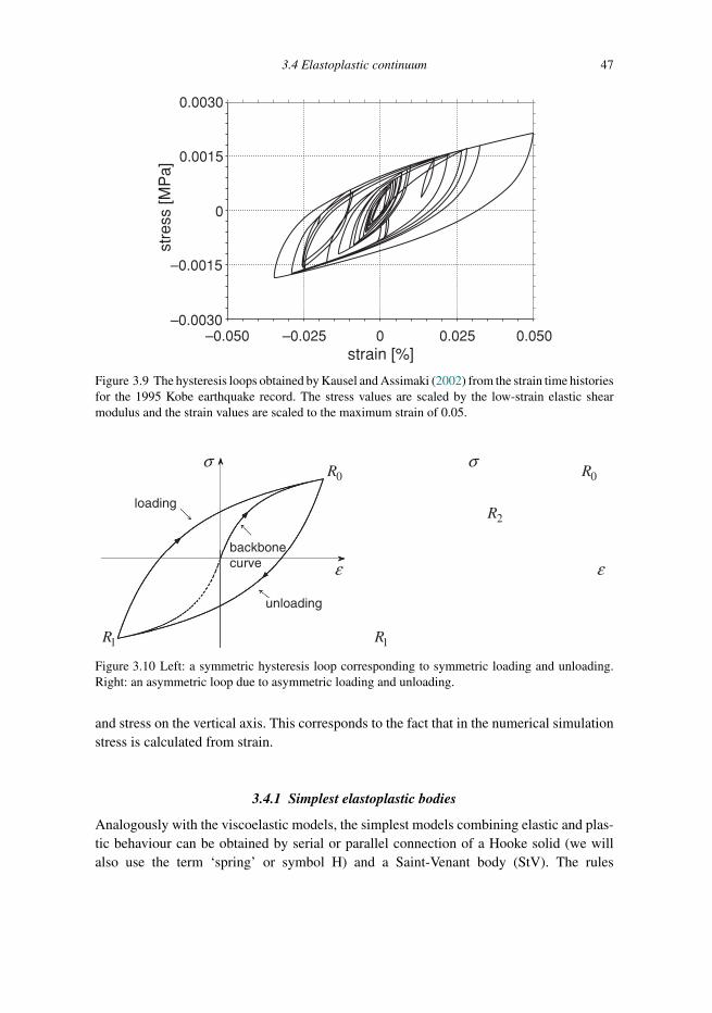
Trim: 247mm × 174mm Top: 14.762mm Gutter: 23.198mmCUUK2497-03 CUUK2497/Moczo ISBN: 978 1 107 02881 4 November 14, 2013 19:53
3.4 Elastoplastic continuum 47
–0.050 –0.025 0 0.025 0.050
0.0030
0.0015
0
–0.0015
–0.0030
stre
ss [M
Pa]
strain [%]
Figure 3.9 The hysteresis loops obtained by Kausel and Assimaki (2002) from the strain time historiesfor the 1995 Kobe earthquake record. The stress values are scaled by the low-strain elastic shearmodulus and the strain values are scaled to the maximum strain of 0.05.
0R
1R
2R
1R
0R
ε ε
σ σ
loading
backbonecurve
unloading
Figure 3.10 Left: a symmetric hysteresis loop corresponding to symmetric loading and unloading.Right: an asymmetric loop due to asymmetric loading and unloading.
and stress on the vertical axis. This corresponds to the fact that in the numerical simulationstress is calculated from strain.
3.4.1 Simplest elastoplastic bodies
Analogously with the viscoelastic models, the simplest models combining elastic and plas-tic behaviour can be obtained by serial or parallel connection of a Hooke solid (we willalso use the term ‘spring’ or symbol H) and a Saint-Venant body (StV). The rules

Trim: 247mm × 174mm Top: 14.762mm Gutter: 23.198mmCUUK2497-03 CUUK2497/Moczo ISBN: 978 1 107 02881 4 November 14, 2013 19:53
48 Rheological models of a continuum
,σ ε ,σ ε
MYσ
Yσ
M
Figure 3.11 Left: H-s-StV – serial connection of a Hooke solid (spring) and a Saint-Venant body.Right: H-p-StV – parallel connection of a Hooke solid and a Saint-Venant body.
σ
Yσ
1σ
ε1ε
σ
Yσ
Yσ−
Yε 1ε ε
Figure 3.12 Left: stress–strain diagram of H-s-StV. Right: stress–strain diagram of H-p-StV.
for combining rheological models in Section 3.2 are also assumed for the elastoplasticmodels.
Serial connection of a Hooke solid and a Saint-Venant body; H-s-StV The rheologicalmodel is shown in Fig. 3.11(left). Stresses are equal, strains are additive:
σ = σH = σStV, ε = εH + εStV (3.143)
Consider, for instance, pulling to the right. The following development is illustrated by thestress–strain diagram in Fig. 3.12(left). If the applied stress is smaller than the yield stressσY of StV, only the spring deforms (extends) – strain linearly increases with stress. Whenthe applied stress reaches a value of σY , StV starts deforming (moving to the right) andthe spring stops deforming. If the loading stress does not decrease below σY , the strainincreases (at a constant σ = σY ) to a value that depends only on the time duration of thestress application and the strain of the spring is equal to εY . With the spring inactive, thestrain of StV increases until the value of the applied stress starts decreasing. We denotethe total strain reached by ε1. As soon as the applied stress starts decreasing, StV stopsdeforming (its strain is ε1 − εY ) and the spring is activated. With StV inactive, the strain ofthe spring linearly decreases. Consequently, the total strain also decreases linearly. Whenthe stress decreases down to zero, the spring has no stress and no strain. The total strain is

Trim: 247mm × 174mm Top: 14.762mm Gutter: 23.198mmCUUK2497-03 CUUK2497/Moczo ISBN: 978 1 107 02881 4 November 14, 2013 19:53
3.4 Elastoplastic continuum 49
equal to the strain of StV, that is, ε1 − εY . If the stress further decreases, the spring startsshrinking. When the stress reaches a value of −σY , StV starts deforming – moving to theleft. At the same time, the spring stops deforming because StV is active at the constantstress −σY . It is obvious that in H-s-StV the episodes of active spring (linear segments ofthe stress–strain diagram) may alternate with episodes of active StV (horizontal segments).It is also clear that H-s-StV does not exhibit plastic strain hardening. In this aspect it doesnot differ from StV itself, which is a mechanical model for the behaviour of an ideal orpure plastic material (see Subsection 3.1.3).
Parallel connection of Hooke solid and Saint-Venant body: H-p-StV The rheologicalmodel is shown in Fig. 3.11(right). Stresses are additive, strains are equal:
σ = σH + σStV, ε = εH = εStV (3.144)
Consider again pulling to the right. The following development is illustrated by the stress–strain diagram in Fig. 3.12(right). Because the strain at H, the strain at StV and the totalstrain are equal at any time, the body is inactive until the stress at StV reaches the yield stressσY . After the stress reaches a value of σY , both H and StV start deforming simultaneously.The deformation is controlled by H. Because StV can deform at the constant stress σY ,the strain is proportional to the difference σ − σY acting at H. (Note that because both Hand StV are active simultaneously, H-p-StV exhibits plastic strain hardening.) Assume thatafter some time the stress reaches a value of σ1. The corresponding strain is (σ1 − σY )/M ,the stress at H is σ1 − σY , and the stress at StV is σY . Assume that at this moment the stressstarts decreasing. This instantaneously stops deformation of both H and StV. The decreaseof the total stress reduces stress only at StV because at inactive H neither strain nor stress canchange. Consequently, both bodies will remain inactive until stress at StV reaches the yieldvalue of −σY . The total stress at that moment is σ1 − 2σY . Note that during the episode withboth bodies inactive the strain was constant although the stress was decreasing. As soon asboth bodies are activated, the strain linearly decreases with decreasing stress. It is obviousthat in H-p-StV the episodes with both bodies active (linear segments of the stress–straindiagram) may alternate with episodes with both bodies inactive (vertical segments in thestress–strain diagram).
Partial conclusion We can see the consequence and drawback of the serial connection ofH and StV: after the applied stress reaches the value of the yield stress, strain increases atthis stress until the applied stress starts decreasing. In other words, the model is not capableof plastic strain hardening. The consequence and drawback of the parallel connection of Hand StV is that the model behaves as a rigid solid before the applied stress reaches the yieldstress. The main advantage of the parallel connection is that both H and StV are active atthe same time.
An indirect indication from the behaviour of both connections is to combine the serialand parallel connections. There are several possibilities. For example, if we connect H-p-StV in series with a spring, we add the capability of an instantaneous elastic responseto the behaviour of H-p-StV. As a consequence, we remove the vertical segments in the
Trim: 247mm × 174mm Top: 14.762mm Gutter: 23.198mmCUUK2497-03 CUUK2497/Moczo ISBN: 978 1 107 02881 4 November 14, 2013 19:53
50 Rheological models of a continuum
stress–strain diagram. Such a connection is used in the sophisticated and flexible modeldeveloped by Iwan (1967).
3.4.2 Iwan elastoplasic model for hysteretic stress–strain behaviour
3.4.2.1 Preliminary considerations
Serial connection of springs Consider first N + 1 springs connected in series. LetMk bethe elastic modulus of the k-th spring. Obviously, application of stress to a body consistingof springs connected in series instantaneously and simultaneously activates all the springs.Consider some reference state of stress and strain at some time:
σ r = σ rH,k, εr =∑N
k=0εrH,k =
∑N
k=0
σ r
Mk(3.145)
At some later time, due to an increment �σ in stress, the stress and strain are
σ = σ r +�σ
ε = εr +�ε = εr +∑N
k=0
�σ
Mk= εr + (σ − σ r )
∑N
k=0
1
Mk(3.146)
Serial connection of the H-p-StV bodies Consider nowN + 1 H-p-StV bodies connectedin series. Let Mk be an elastic modulus of the kth spring and σY,k a yield stress of the kthStV. Without loss of generality consider
σY,0 < σY,1 < · · · < σY,N (3.147)
At each (H–p–StV)k at any time,
σk = σH,k + σStV,k = σ, εk = εH,k = εStV,k (3.148)
In general, we are interested in cyclic variation of the applied stress: not only the size butalso the direction of the stress varies. The applied stress can reverse (change its direction)at any time. The application of stress in the positive direction may be called loading, theapplication of stress in the negative direction may be called unloading (see Fig. 3.10, left).A point at which the stress changes direction is a reversal point. Note that at each reversalpoint all elements of the model are deactivated. A curve connecting two successive reversalpoints is called a branch.
Contrary to the body consisting of springs connected in series, application of stress toa serial connection of several H-p-StV bodies does not necessarily activate one or moreH–p–StV bodies. (H–p–StV)k is activated in the positive direction when σStV,k = σY,k andin the negative direction when σStV,k = −σY,k . The total stress at which (H–p–StV)k isactivated may be called the the activating stress. It follows from the first of Eqs. (3.148)that the activating stresses for the two directions can be defined as
�σAk ≡ σH,k + σY,k, ←σA
k ≡ σH,k − σY,k (3.149)
Note that the orientation of the arrow indicates the direction of the applied stress.

Trim: 247mm × 174mm Top: 14.762mm Gutter: 23.198mmCUUK2497-03 CUUK2497/Moczo ISBN: 978 1 107 02881 4 November 14, 2013 19:53
3.4 Elastoplastic continuum 51
0M
,2Yσ
2M
,1Yσ
1M
,σ ε,Y Nσ
NM
Figure 3.13 Iwan elastoplastic model.
Consider some state of stress and strain as a reversal point, and denote it by [σR, εR].The first of Eqs. (3.148) and Eqs. (3.149) imply
�σAk = σR − σRStV,k + σY,k, ←σA
k = σR − σRStV,k − σY,k (3.150)
where the upper index R indicates the reversal point.
3.4.2.2 Iwan model
Assume that σY,0 = 0 in the above serial connection of the H-p-StV bodies. In other words,(H–p–StV)0 reduces to a spring H0. Consequently, we have a single spring H0 connectedin series with the serial connection of (H–p–StV)k; k = 1, . . . , N . This is the Iwan model(Fig. 3.13). The reduction of (H–p–StV)0 to a single spring incorporates the capability ofan elastic response.
Consider an initial state with σ = 0 and ε = 0. The following development is illustratedin Fig. 3.14. Assume application of stress σ in the positive direction (to the right) and
σY,K0 ≤ σ < σY,K0+1 (3.151)
This means that K0 H-p-StV bodies are activated. H0 and each of (H–p–StV)k; k =1, . . . , K0 contribute to the total strain proportionally to the difference σ − σY,k andinversely proportionally toMk:
ε =∑K0
k=0
σ − σY,kMk
(3.152)
Note that for conciseness we formally included also the zero-valued σY,0.Assume reversal at the state characterized by Eqs. (3.151) and (3.152), and denote the
stress and strain at that state by σR0 and εR0 :
εR0 =∑K0
k=0
σR0 − σY,kMk
(3.153)
(The stress–strain curve connecting the initial state [σ = 0, ε = 0] with the reversal point[σR0 , εR0 ] is part of the backbone curve.)
We have to realize now that the next reversal of the stress may occur even before anyof the H-p-StV bodies are activated during unloading. It may also happen that only someof the H-p-StV bodies activated during loading are activated during the unloading. For allpossible developments we need to find the activating stresses in both directions.
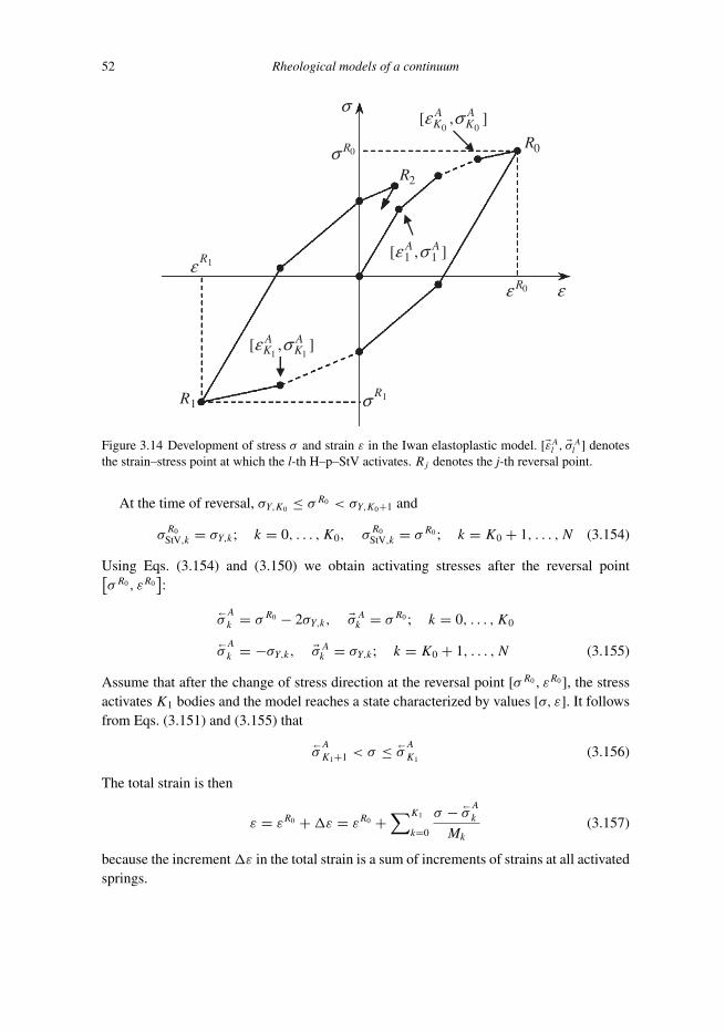
Trim: 247mm × 174mm Top: 14.762mm Gutter: 23.198mmCUUK2497-03 CUUK2497/Moczo ISBN: 978 1 107 02881 4 November 14, 2013 19:53
52 Rheological models of a continuum
σ
ε
0Rσ
0Rε
1Rε
1Rσ
1 1[ , ]A A
K Kε σ
0R
1R
2R
1 1[ , ]A Aε σ
0 0[ , ]A A
K Kε σ
Figure 3.14 Development of stress σ and strain ε in the Iwan elastoplastic model. [�εAl , �σAl ] denotesthe strain–stress point at which the l-th H–p–StV activates. Rj denotes the j-th reversal point.
At the time of reversal, σY,K0 ≤ σR0 < σY,K0+1 and
σR0StV,k = σY,k; k = 0, . . . , K0, σ
R0StV,k = σR0 ; k = K0 + 1, . . . , N (3.154)
Using Eqs. (3.154) and (3.150) we obtain activating stresses after the reversal point[σR0 , εR0
]:
←σA
k = σR0 − 2σY,k, �σAk = σR0 ; k = 0, . . . , K0
←σA
k = −σY,k, �σAk = σY,k; k = K0 + 1, . . . , N (3.155)
Assume that after the change of stress direction at the reversal point [σR0 , εR0 ], the stressactivates K1 bodies and the model reaches a state characterized by values [σ, ε]. It followsfrom Eqs. (3.151) and (3.155) that
←σA
K1+1 < σ ≤ ←σA
K1(3.156)
The total strain is then
ε = εR0 +�ε = εR0 +∑K1
k=0
σ − ←σA
k
Mk(3.157)
because the increment�ε in the total strain is a sum of increments of strains at all activatedsprings.

Trim: 247mm × 174mm Top: 14.762mm Gutter: 23.198mmCUUK2497-03 CUUK2497/Moczo ISBN: 978 1 107 02881 4 November 14, 2013 19:53
3.4 Elastoplastic continuum 53
Consider now the state reached as a reversal point [σR1 , εR1 ]:
εR1 = εR0 +∑K1
k=0
σR1 − ←σA
k
Mk(3.158)
As mentioned before, at the reversal point all elements of the model are deactivated.Therefore, we need to find activating stresses after the reversal point R1. Recalling Eqs.(3.150) and distinguishing two possible cases we obtain
K1 < K0
k = 0, . . . , K1 : σR1StV,k = −σY,k
�σAk = σR1 + 2σY,k,←σA
k = σR1
k = K1 + 1, . . . , K0 : σR1StV,k = σY,k − (σR0 − σR1 )
�σAk = σR0 ,←σA
k = σR0 − 2σY,k
k = K0 + 1, . . . , N : σR1StV,k = σR1
�σAk = σY,k, ←σA
k = −σY,k
(3.159)
K1 ≥ K0
k = 0, . . . , K0 : σR1StV,k = −σY,k
�σAk = σR1 + 2σY,k,←σA
k = σR1
k = K0 + 1, . . . , K1 : σR1StV,k = −σY,k
�σAk = σR1 + 2σY,k,←σA
k = σR1
k = K1 + 1, . . . , N : σR1StV,k = σR1
�σAk = σY,k, ←σA
k = −σY,k
(3.160)
Compare now the activating stresses after the reversal point R1 with those after point R0.We can see different activating stresses only for those H-p-StV that were activated betweenR0 and R1. (Note that it was not necessary to calculate activating stresses for H-p-StV notactivated between R0 and R1.)
Assume that after the change of stress direction at the reversal point [σR1 , εR1 ], the stressactivates K2 bodies and the model reaches a state characterized by values [σ, ε] and
�σAK2≤ σ < �σAK2+1 (3.161)
The total strain is then
ε = εR1 +�ε = εR1 +∑K2
k=0
σ − �σAkMk
(3.162)
We have shown the calculation of strain for the first loading along the backbone curve, thefirst unloading, and the second loading. It would be easy to continue if the state reachedbecomes a reversal point.
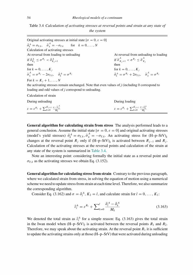
Trim: 247mm × 174mm Top: 14.762mm Gutter: 23.198mmCUUK2497-03 CUUK2497/Moczo ISBN: 978 1 107 02881 4 November 14, 2013 19:53
54 Rheological models of a continuum
Table 3.4 Calculation of activating stresses at reversal points and strain at any state ofthe system
Original activating stresses at initial state [σ = 0, ε = 0]
�σAk = σY,k, ←σA
k = −σY,k for k = 0, . . . , NCalculation of activating stressesAt reversal from loading to unloading At reversal from unloading to loading
if �σAKj ≤ σRj < �σAKj+1
thenfor k = 0, . . . , Kj←σA
k = σRj − 2σY,k, �σAk = σRj
if ←σA
Kj+1 < σRj ≤ ←
σA
Kj
thenfor k = 0, . . . , Kj�σAk = σRj + 2σY,k,
←σA
k = σRjFor k = Kj + 1, . . . , Nthe activating stresses remain unchanged. Note that even values of j (including 0 correspond toloading and odd values of j correspond to unloading.
Calculation of strain
During unloading During loading
ε = εRj +∑Kj+1k=0
σ−←σAk
Mkε = εRj +∑Kj+1
k=0σ−�σAkMk
General algorithm for calculating strain from stress The analysis performed leads to ageneral conclusion. Assume the initial state [σ = 0, ε = 0] and original activating stresses(model’s yield stresses) �σAk = σY,k, ←
σA
k = −σY,k . An activating stress for (H–p–StV)kchanges at the reversal point Rj only if (H–p–StV)k is activated between Rj−1 and Rj .Calculation of the activating stresses at the reversal points and calculation of the strain atany state of the system is summarized in Table 3.4.
Note an interesting point: considering formally the initial state as a reversal point andσY,k as the activating stresses we obtain Eq. (3.152).
General algorithm for calculating stress from strain Contrary to the previous paragraph,where we calculated strain from stress, in solving the equation of motion using a numericalscheme we need to update stress from strain at each time level. Therefore, we also summarizethe corresponding algorithm.
Consider Eq. (3.162) and σ = �σAl ,K2 = l, and calculate strain for l = 0, . . . , K1:
�εAl = εR1 +∑l
k=0
�σAl − �σAkMk
(3.163)
We denoted the total strain as �εAl for a simple reason: Eq. (3.163) gives the total strainin the Iwan model when (H–p–StV)l is activated between the reversal points R1 and R2.Therefore, we may speak about the activating strain. At the reversal point R1 it is sufficientto update the activating strains only at those (H–p–StV) that were activated during unloading
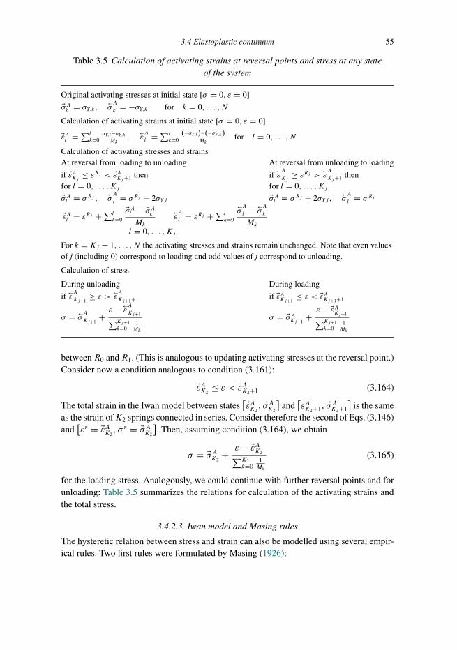
Trim: 247mm × 174mm Top: 14.762mm Gutter: 23.198mmCUUK2497-03 CUUK2497/Moczo ISBN: 978 1 107 02881 4 November 14, 2013 19:53
3.4 Elastoplastic continuum 55
Table 3.5 Calculation of activating strains at reversal points and stress at any stateof the system
Original activating stresses at initial state [σ = 0, ε = 0]
�σAk = σY,k, ←σA
k = −σY,k for k = 0, . . . , N
Calculation of activating strains at initial state [σ = 0, ε = 0]
�εAl = ∑lk=0
σY,l−σY,kMk
,←εA
l = ∑lk=0
(−σY,l)−(−σY,k)Mk
for l = 0, . . . , N
Calculation of activating stresses and strainsAt reversal from loading to unloading At reversal from unloading to loading
if �εAKj ≤ εRj < �εAKj+1 thenfor l = 0, . . . , Kj�σAl = σRj , ←
σA
l = σRj − 2σY,l
if ←εA
Kj≥ εRj > ←
εA
Kj+1 thenfor l = 0, . . . , Kj�σAl = σRj + 2σY,l,
←σA
l = σRj
�εAl = εRj +∑lk=0
�σAl − �σAkMk
←εA
l = εRj +∑lk=0
←σA
l − ←σA
k
Mk
l = 0, . . . , Kj
For k = Kj + 1, . . . , N the activating stresses and strains remain unchanged. Note that even valuesof j (including 0) correspond to loading and odd values of j correspond to unloading.
Calculation of stress
During unloading During loading
if ←εA
Kj+1≥ ε > ←
εA
Kj+1+1 if �εAKj+1≤ ε < �εAKj+1+1
σ = ←σA
Kj+1+ε − ←
εA
Kj+1∑Kj+1k=0
1Mk
σ = �σAKj+1+ε − �εAKj+1∑Kj+1k=0
1Mk
between R0 and R1. (This is analogous to updating activating stresses at the reversal point.)Consider now a condition analogous to condition (3.161):
�εAK2≤ ε < �εAK2+1 (3.164)
The total strain in the Iwan model between states[�εAK2
, �σAK2
]and
[�εAK2+1, �σAK2+1
]is the same
as the strain ofK2 springs connected in series. Consider therefore the second of Eqs. (3.146)and
[εr = �εAK2
, σ r = �σAK2
]. Then, assuming condition (3.164), we obtain
σ = �σAK2+ ε − �εAK2∑K2
k=01Mk
(3.165)
for the loading stress. Analogously, we could continue with further reversal points and forunloading: Table 3.5 summarizes the relations for calculation of the activating strains andthe total stress.
3.4.2.3 Iwan model and Masing rules
The hysteretic relation between stress and strain can also be modelled using several empir-ical rules. Two first rules were formulated by Masing (1926):

Trim: 247mm × 174mm Top: 14.762mm Gutter: 23.198mmCUUK2497-03 CUUK2497/Moczo ISBN: 978 1 107 02881 4 November 14, 2013 19:53
56 Rheological models of a continuum
0
5
10
15
20
25
30
35
0
0.2
0.4
0.6
0.8
1
0.0001 0.001 0.01 0.1 1
Dam
pin
g R
atio
(%
)
Shear Strain (%)
Shear Modulus
Damping (%)
CalculatedDamping Ratio
Shear strain [%]
G /
Gs
max
Shear modulus
Damping
Calculateddamping ratio
ms
m
Gσε
=
mσ
mε
maxG
tG
sG
Dam
ping ratio [%]
Figure 3.15 Left: modulus reduction curve, calculated and measured damping ratio. Right: secantshear modulus Gs , tangential shear modulus Gt and the elastic modulus Gmax.
(1) For initial loading, the stress–strain curve follows the backbone curve σ = Fbb(ε).(2) If stress reversal occurs at a point defined by (εR, σR), the stress–strain curve follows
a path given by 12 (σ − σR) = Fbb( 1
2 (ε − εR)). In other words, the unloading and load-ing curves have the same shape as the backbone curve (with the origin shifted to thereversal point) enlarged by a factor of two.
The two Masing rules are sufficient in the case of cyclic loading between two fixed limits.However, their application in the case of irregular loads gives a curve that is different fromthe experimentally found curve. Therefore, two more rules were formulated (e.g., Kramer1996):
(3) If the unloading or reloading curve exceeds the maximum past strain and intersects thebackbone curve, it follows the backbone curve until the next stress reversal.
(4) If an unloading or reloading curve crosses an unloading or reloading curve from theprevious cycle, the stress–strain curve follows that of the previous cycle.
The four rules are called the extended Masing rules. It is worth noting that the Iwan modelis consistent with all four rules, although the third and fourth rules were formulated afterIwan’s (1967) article.
3.4.2.4 Determination of parameters for Iwan model
As shown previously, (H–p–StV)k is activated when the loading stress reaches a value ofσY,k . Activation of the spring with elastic modulusMk changes the slope of the stress–straincurve. This means that the shear modulus of the Iwan model changes (it decreases). Thetangential shear modulus is defined (Joyner and Chen 1975) as
Gt = σY,k+1 − σkεY,k+1 − εY,k =
(∑k
i=0
1
Mi
)−1
(3.166)
In practice, the decrease of the shear modulus is characterized by the modulus reductioncurve (Fig. 3.15, left) that shows normalized secant shear modulusGs/Gmax as a function of

Trim: 247mm × 174mm Top: 14.762mm Gutter: 23.198mmCUUK2497-03 CUUK2497/Moczo ISBN: 978 1 107 02881 4 November 14, 2013 19:53
3.4 Elastoplastic continuum 57
strain.Gmax is the elastic modulus and the secant modulus is illustrated in Fig. 3.15(right).Assume, for instance, that the true modulus reduction curve is reasonably piece-wiselinearly approximated by a set of [εi, (Gs/Gmax)i] measured points. Then, see Fig. 3.15,
σY,i = GsεY,i = (Gs/Gmax)i GmaxεY,i (3.167)
Having determined all yield stresses and corresponding strains, we can iteratively userelation (3.166) to calculate the elastic moduliMi .
3.4.2.5 Note on damping
Damping, the ratio of the dissipated energy and the maximum strain energy stored in thesystem, see Eq. (3.69), is an inherent property of the Iwan model (beyond the first elasticpart of the backbone curve). For a given strain εm the dissipated energy is equal to area ofthe symmetrical hysteresis loop – see Fig. 3.15(right). The Iwan model has no damping atlow strains but its value at high strains could be larger than the measured damping. The firstproblem can be solved by including linear viscoelasticity, the second problem by changingloading/unloading paths according to specified damping values, as proposed by Muravskii(2005).
The Iwan model, as described in this chapter, is applicable in the case of interme-diate strains. If possible, in order to check the validity of the procedure, it is recom-mended to check the damping corresponding to the maximum strain computed during wavepropagation.
3.4.2.6 Concluding remark
In the section on the elastoplastic continuum we introduced only the basics of the nonlinearhysteretic behaviour of soft soil at moderate and large strains. The possibility of hystereticbehaviour considerably complicates numerical prediction of earthquake motion. If thecomputational domain includes a part with possibly nonlinear behaviour, the numericalscheme should be capable of accounting for such behaviour in order to produce realisticpredictions. At present, this is still a nontrivial task for 3D numerical modelling.
We finish this section by mentioning two impressive studies. Gelis and Bonilla (2012)considered elastic, viscoelastic, elastoplastic and viscoelastoplastic rheologies, and investi-gated the influence of rheology on seismic motion. They concluded that numerical simula-tions should couple both viscoelasticity (to account for energy dissipation at small strains)and nonlinearity (to account for hysteretic energy dissipation and shear modulus degrada-tion at higher strains) in order to obtain realistic results. Gelis and Bonilla also investigatedthe effect of the input motion on the development of nonlinear behaviour. For modellingand numerical implementation of nonlinear hysteretic behaviour we also refer to the com-prehensive article by Assimaki et al. (2008). Both articles refer to other recent studies ofnonlinear behaviour.

Trim: 247mm × 174mm Top: 14.762mm Gutter: 23.198mmCUUK2497-04 CUUK2497/Moczo ISBN: 978 1 107 02881 4 November 14, 2013 20:31
4
Earthquake source
In this chapter we will focus on seismic radiation as emitted from a rupturing fault in theEarth. On a large scale, due to tectonic loading the stress in the fault area increases until theyield stress of the rock material is reached at some point in the fault zone. Reaching yieldstress leads to nonelastic deformation and to release of deformation energy. This increasesstress in the vicinity of the point. Reaching the yield stress at the neighbouring points mayconsequently lead to a chain reaction – rupture propagation. When the rupture propagatesfast enough and in a nonsteady way it radiates seismic waves which then propagate awayfrom the fault. Note that seismic waves are radiated only if the rupture propagation speedis a significant fraction of the S-wave speed; slow ruptures do not radiate. Note also thatsubshear steady-state slip pulses do not radiate, except at their starting and stopping points;radiation from subshear ruptures requires nonsteady slip. Rupture propagates on the faultas long as the stress changes associated with the propagating rupture are large enough forthe stress at points in front of the crack tip to reach the yield stress.
The earthquake fault is usually considered a frictional contact. Therefore, friction is themost important physical phenomenon during rupture nucleation and propagation. However,there are many other physical processes that have an impact on the effective friction, e.g.,thermal pressurization of pore fluids, flash heating and melting of the material in the faultzone, nonelastic deformation (plasticity, crack formation, gouge formation), as summarizedby Bizzarri (2010) and Bizzarri and Cocco (2005), for example. It has been shown thatheterogeneous friction parameters (e.g., Ampuero et al. 2006, Liu and Lapusta 2008, Tintiet al. 2005, 2009), geometrical complexity (e.g., Oglesby and Day 2001, Oglesby et al. 2008,Oglesby and Mai 2012), and fault roughness (Dunham et al. 2011) may also significantlyimpact the rupture behaviour. Rupture propagation on faults at the contact of two differentmaterials, the so-called bi-material faults, has also been intensively studied (e.g., Andrewsand Ben-Zion 1997, Harris and Day 1997, Ben-Zion and Andrews 1998, Ranjith and Rice2001, Rubin and Ampuero 2007, Ampuero and Ben-Zion 2008).
We can use a dynamic or kinematic model of the earthquake source. These models differmainly in how they respect the physics. The temporal and spatial evolution of the slip ratein the dynamic model is calculated by solving an equation of motion together with thefriction law, and possibly other physical laws (in order to explicitly include, for instance,pore pressure or temperature). Consequently, the interaction between rupture and wavefield
58

Trim: 247mm × 174mm Top: 14.762mm Gutter: 23.198mmCUUK2497-04 CUUK2497/Moczo ISBN: 978 1 107 02881 4 November 14, 2013 20:31
4.1 Dynamic model of an earthquake source 59
fault
Figure 4.1 Fault surface and the normal vector �n.
is implicitly included. Therefore, we can consider the resulting slip-rate functions in thedynamic model to be physically consistent. On the other hand, the kinematic model isdescribed by the temporal and spatial evolution of the slip rate. The slip-rate evolution isprescribed a priori and is not interacting with the stress changes induced by the rupturepropagation. Therefore, the kinematic model may be inconsistent with known friction laws(this depends on how the slip-rate evolution was obtained). It is to be noted, however, thatlarge uncertainties remain about the physics of fault friction at natural scales. In the nextsections we will describe the models in more detail.
In order to use a source model in a numerical simulation we need to know values ofthe model parameters. The parameter set will be different for different types of sourcemodel but, in general, the parameters should be estimated from the observations. Differentapproaches are used to derive parameters of the point, finite-fault kinematic and dynamicsource models from observations, although some of these parameters are poorly constrained(e.g., Ide 2009, Guatteri and Spudich 2000). However, this represents a very wide topic(which does not fit into the content of this book) and we refer the reader to, e.g., Dziewonskiet al. (1981), Sipkin (1982), Langston et al. (1982), Olson and Apsel (1982), Hartzell andHeaton (1983), Peyrat et al. (2001), Liu and Archuleta (2004), Monelli et al. (2009), Festaand Zollo (2012), Di Carli et al. (2010).
4.1 Dynamic model of an earthquake source
In many seismological problems an earthquake fault may be represented by a surfaceembedded in a heterogeneous elastic or viscoelastic pre-stressed medium. Nonzero initialstress is due to tectonic loading and residual stress after previous earthquakes on the fault.An earthquake source itself may be modelled as spontaneous rupture propagation alongthe fault. The rupture generates seismic waves, which then propagate from the fault intothe embedding medium. Inside the rupture, displacement and particle-velocity vectors arediscontinuous across the fault. At the same time, traction is continuous. Let �n (�x) be a unitnormal vector to the fault surface pointing from the ‘−’ to the ‘+’ side of the surface(Fig. 4.1).
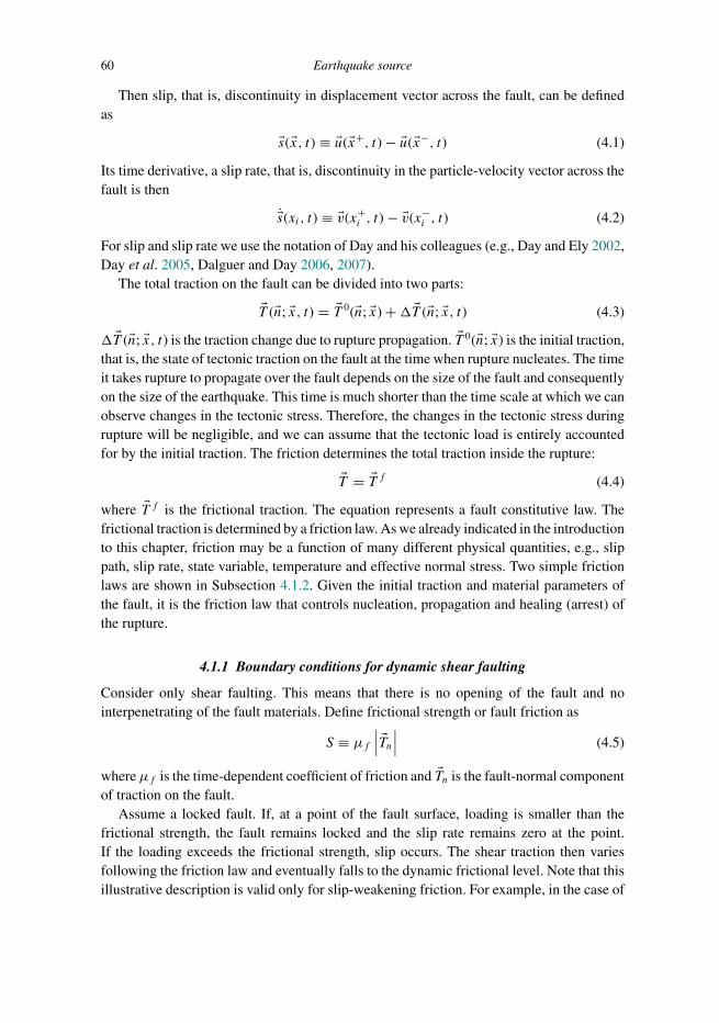
Trim: 247mm × 174mm Top: 14.762mm Gutter: 23.198mmCUUK2497-04 CUUK2497/Moczo ISBN: 978 1 107 02881 4 November 14, 2013 20:31
60 Earthquake source
Then slip, that is, discontinuity in displacement vector across the fault, can be definedas
�s(�x, t) ≡ �u(�x+, t) − �u(�x−, t) (4.1)
Its time derivative, a slip rate, that is, discontinuity in the particle-velocity vector across thefault is then
�s(xi, t) ≡ �v(x+i , t) − �v(x−
i , t) (4.2)
For slip and slip rate we use the notation of Day and his colleagues (e.g., Day and Ely 2002,Day et al. 2005, Dalguer and Day 2006, 2007).
The total traction on the fault can be divided into two parts:
�T (�n; �x, t) = �T 0(�n; �x) +� �T (�n; �x, t) (4.3)
� �T (�n; �x, t) is the traction change due to rupture propagation. �T 0(�n; �x) is the initial traction,that is, the state of tectonic traction on the fault at the time when rupture nucleates. The timeit takes rupture to propagate over the fault depends on the size of the fault and consequentlyon the size of the earthquake. This time is much shorter than the time scale at which we canobserve changes in the tectonic stress. Therefore, the changes in the tectonic stress duringrupture will be negligible, and we can assume that the tectonic load is entirely accountedfor by the initial traction. The friction determines the total traction inside the rupture:
�T = �T f (4.4)
where �T f is the frictional traction. The equation represents a fault constitutive law. Thefrictional traction is determined by a friction law. As we already indicated in the introductionto this chapter, friction may be a function of many different physical quantities, e.g., slippath, slip rate, state variable, temperature and effective normal stress. Two simple frictionlaws are shown in Subsection 4.1.2. Given the initial traction and material parameters ofthe fault, it is the friction law that controls nucleation, propagation and healing (arrest) ofthe rupture.
4.1.1 Boundary conditions for dynamic shear faulting
Consider only shear faulting. This means that there is no opening of the fault and nointerpenetrating of the fault materials. Define frictional strength or fault friction as
S ≡ μf∣∣∣ �Tn∣∣∣ (4.5)
whereμf is the time-dependent coefficient of friction and �Tn is the fault-normal componentof traction on the fault.
Assume a locked fault. If, at a point of the fault surface, loading is smaller than thefrictional strength, the fault remains locked and the slip rate remains zero at the point.If the loading exceeds the frictional strength, slip occurs. The shear traction then variesfollowing the friction law and eventually falls to the dynamic frictional level. Note that thisillustrative description is valid only for slip-weakening friction. For example, in the case of

Trim: 247mm × 174mm Top: 14.762mm Gutter: 23.198mmCUUK2497-04 CUUK2497/Moczo ISBN: 978 1 107 02881 4 November 14, 2013 20:31
4.1 Dynamic model of an earthquake source 61
rate-and-state friction, the shear traction is always equal to the frictional strength and thefault is always slipping.
Let subscripts sh and n denote the shear and normal components with respect to the faultsurface. The boundary conditions on the fault can be formulated as follows (Day 1982, Dayet al. 2005).
Shear faulting
�sn = 0, �sn = 0, �ssh = 0, �ssh = 0 (4.6)
Shear traction bounded by the frictional strength∣∣∣ �Tsh∣∣∣ ≤ S (4.7)
Colinearity of the shear traction and slip rate
�Tsh(�n) = S �ssh∣∣�ssh∣∣ (4.8)
The slip is opposed by the friction. The fact that the frictional traction opposes the slip isconsistent with the colinearity requirement because (1) we consider vector �n to be orientedin the direction from the ‘−’ to the ‘+’ side of the fault (that is, �T (�n) characterizes tractionwith which the ‘+’ side acts on the ‘−’ side of the fault), (2) we consider slip as the relativemotion of the ‘+’ side with respect to the ‘−’ side of the fault. Thus �T (�n) and slip have thesame direction. If slip was defined as the relative motion of the ‘−’ side with respect to the‘+’ side of the fault, the requirement of the antiparallelism with the ‘−’ sign on the r.h.s.of Eq. (4.8) would be consistent with frictional traction opposing the relative motion of thefault faces.
4.1.2 Friction law
When a rupture front reaches a point of the fault and slip starts at that point (that is, thetwo originally neighbouring points, one at the ‘−’ and the other at the ‘+’ side of the fault,start slipping), the total dynamic traction varies according to a constitutive law that relatesstress change and frictional behaviour, and eventually falls to the dynamic frictional level.If the variation in traction is gradual (not instantaneous), the traction at the point reachesthe dynamic frictional level during a finite time. During this finite time, points of the faultin front of the considered point may start slipping. Thus, the process of traction degradationobviously occurs within a finite zone behind the so-called crack tip (the rupture frontmostpoint). This zone is termed the cohesive (also breakdown or process) zone. The friction lawdetermines processes and phenomena in the cohesive zone.
Following Bizzarri and Cocco (2005), the coefficient of friction can be a function ofseveral quantities:
μf = μf (l, |�s|, �1, . . . , �N, T ,H, λc, hm, g, Ce) (4.9)
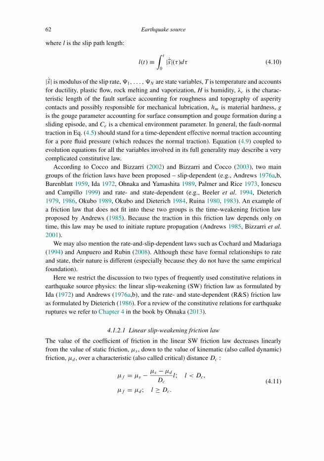
Trim: 247mm × 174mm Top: 14.762mm Gutter: 23.198mmCUUK2497-04 CUUK2497/Moczo ISBN: 978 1 107 02881 4 November 14, 2013 20:31
62 Earthquake source
where l is the slip path length:
l(t) ≡∫ t
0|�s|(τ )dτ (4.10)
|�s| is modulus of the slip rate,�1, . . . , �N are state variables, T is temperature and accountsfor ductility, plastic flow, rock melting and vaporization, H is humidity, λc is the charac-teristic length of the fault surface accounting for roughness and topography of asperitycontacts and possibly responsible for mechanical lubrication, hm is material hardness, gis the gouge parameter accounting for surface consumption and gouge formation during asliding episode, and Ce is a chemical environment parameter. In general, the fault-normaltraction in Eq. (4.5) should stand for a time-dependent effective normal traction accountingfor a pore fluid pressure (which reduces the normal traction). Equation (4.9) coupled toevolution equations for all the variables involved in its full generality may describe a verycomplicated constitutive law.
According to Cocco and Bizzarri (2002) and Bizzarri and Cocco (2003), two maingroups of the friction laws have been proposed – slip-dependent (e.g., Andrews 1976a,b,Barenblatt 1959, Ida 1972, Ohnaka and Yamashita 1989, Palmer and Rice 1973, Ionescuand Campillo 1999) and rate- and state-dependent (e.g., Beeler et al. 1994, Dieterich1979, 1986, Okubo 1989, Okubo and Dieterich 1984, Ruina 1980, 1983). An example ofa friction law that does not fit into these two groups is the time-weakening friction lawproposed by Andrews (1985). Because the traction in this friction law depends only ontime, this law may be used to initiate rupture propagation (Andrews 1985, Bizzarri et al.2001).
We may also mention the rate-and-slip-dependent laws such as Cochard and Madariaga(1994) and Ampuero and Rubin (2008). Although these have formal relationships to rateand state, their nature is different (especially because they do not have the same empiricalfoundation).
Here we restrict the discussion to two types of frequently used constitutive relations inearthquake source physics: the linear slip-weakening (SW) friction law as formulated byIda (1972) and Andrews (1976a,b), and the rate- and state-dependent (R&S) friction lawas formulated by Dieterich (1986). For a review of the constitutive relations for earthquakeruptures we refer to Chapter 4 in the book by Ohnaka (2013).
4.1.2.1 Linear slip-weakening friction law
The value of the coefficient of friction in the linear SW friction law decreases linearlyfrom the value of static friction, μs , down to the value of kinematic (also called dynamic)friction, μd , over a characteristic (also called critical) distance Dc :
μf = μs − μs − μdDc
l; l < Dc,
μf = μd ; l ≥ Dc.(4.11)

Trim: 247mm × 174mm Top: 14.762mm Gutter: 23.198mmCUUK2497-04 CUUK2497/Moczo ISBN: 978 1 107 02881 4 November 14, 2013 20:31
4.1 Dynamic model of an earthquake source 63
fric
tiona
l tra
ctio
n
dτ
0τ
sτ
slipcD
Figure 4.2 Linear slip-weakening (SW) friction law.
We can define static (yield) and dynamic (kinematic) frictional shear tractions, res-pectively:
| �T ssh| = μs | �Tn|, | �T dsh| = μd | �Tn| (4.12)
We will also use symbols τs , τd , τ0 and τn for the static, dynamic, initial and normaltractions, respectively:
τs ≡ | �T ssh|, τd ≡ | �T dsh|, τ0 ≡ | �T 0sh|, τn ≡ | �Tn| (4.13)
The linear SW friction law is illustrated in Fig. 4.2.Considering the SW friction law means that the evolution of the traction with slip on the
fault is ‘prescribed’ a priori. We know the static and dynamic tractions before the rupturestarts. We just do not know whether they will actually be reached. That will depend on theevolution of stress on and near the fault, and slip on the fault.
4.1.2.2 Rate- and state-dependent friction law
The value of the coefficient of friction in the R&S friction law depends on the modulus ofthe slip rate |�ssh| and state variable � :
μf = μ(|�ssh|, �)d�
dt= g(|�ssh|, �)
(4.14)

Trim: 247mm × 174mm Top: 14.762mm Gutter: 23.198mmCUUK2497-04 CUUK2497/Moczo ISBN: 978 1 107 02881 4 November 14, 2013 20:31
64 Earthquake source
Figure 4.3 Illustration of the R&S friction law.
We can derive several constitutive relations from Eq. (4.14) using different functional formsfor μ and g (e.g., Beeler et al. 1994). The R&S friction law proposed by Dieterich (1986)is
μf = μr − a ln
(sr
|�ssh|+ 1
)+ b ln
(�sr
L+ 1
)d�
dt= 1 − �|�ssh|
L
(4.15)
Here a, b and L are constitutive parameters, μr is the reference coefficient of friction atthe slip rate value sr . The second equations in (4.14) and (4.15) describe evolution of thestate variable. Note that the most common version of R&S in current use does not havethe +1 terms in Eqs. (4.15). Unlike the SW friction law, the yield and kinematic frictionaltractions are not prescribed a priori, they depend on the slip rate and state variable. Therefore,it is not possible to plot the general figure of the R&S friction law. Figure 4.3 shows onlyan example of how traction may depend on slip for particular parameters (based on Coccoet al. 2004). Though the R&S friction law (4.15) does not explicitly include dependence onthe slip path length, the law yields the slip-weakening, with a short slip-hardening phase, asshown by Cocco and Bizzarri (2002). Cocco and Bizzarri (2002) and Bizzarri and Cocco(2003, 2005) compared the two friction laws in detail.
4.2 Kinematic model of an earthquake source
In many applications, kinematic models are used instead of the dynamic ones. In thefinite-fault kinematic model, rupture propagation is simulated using a set of point sourcesdistributed along the fault surface. Each point source is a body-force equivalent and actsindependently of other point sources. Timing of the point sources along the fault surface and
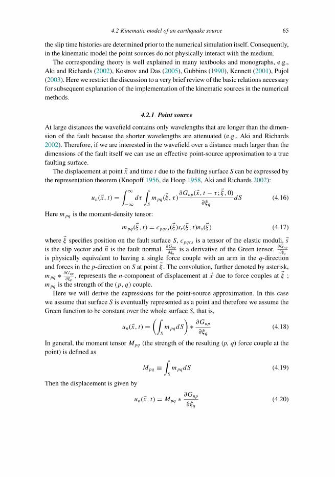
Trim: 247mm × 174mm Top: 14.762mm Gutter: 23.198mmCUUK2497-04 CUUK2497/Moczo ISBN: 978 1 107 02881 4 November 14, 2013 20:31
4.2 Kinematic model of an earthquake source 65
the slip time histories are determined prior to the numerical simulation itself. Consequently,in the kinematic model the point sources do not physically interact with the medium.
The corresponding theory is well explained in many textbooks and monographs, e.g.,Aki and Richards (2002), Kostrov and Das (2005), Gubbins (1990), Kennett (2001), Pujol(2003). Here we restrict the discussion to a very brief review of the basic relations necessaryfor subsequent explanation of the implementation of the kinematic sources in the numericalmethods.
4.2.1 Point source
At large distances the wavefield contains only wavelengths that are longer than the dimen-sion of the fault because the shorter wavelengths are attenuated (e.g., Aki and Richards2002). Therefore, if we are interested in the wavefield over a distance much larger than thedimensions of the fault itself we can use an effective point-source approximation to a truefaulting surface.
The displacement at point �x and time t due to the faulting surface S can be expressed bythe representation theorem (Knopoff 1956, de Hoop 1958, Aki and Richards 2002):
un(�x, t) =∫ ∞
−∞dτ
∫S
mpq(�ξ, τ )∂Gnp(�x, t − τ ; �ξ, 0)
∂ξqdS (4.16)
Here mpq is the moment-density tensor:
mpq(�ξ, t) = cpqrs(�ξ )sr (�ξ, t)ns(�ξ ) (4.17)
where �ξ specifies position on the fault surface S, cpqrs is a tensor of the elastic moduli, �sis the slip vector and �n is the fault normal. ∂Gnp
∂ξqis a derivative of the Green tensor. ∂Gnp
∂ξq
is physically equivalent to having a single force couple with an arm in the q-directionand forces in the p-direction on S at point �ξ . The convolution, further denoted by asterisk,mpq ∗ ∂Gnp
∂ξq, represents the n-component of displacement at �x due to force couples at �ξ ;
mpq is the strength of the (p, q) couple.Here we will derive the expressions for the point-source approximation. In this case
we assume that surface S is eventually represented as a point and therefore we assume theGreen function to be constant over the whole surface S, that is,
un(�x, t) =(∫
S
mpqdS
)∗ ∂Gnp∂ξq
(4.18)
In general, the moment tensorMpq (the strength of the resulting (p, q) force couple at thepoint) is defined as
Mpq ≡∫S
mpqdS (4.19)
Then the displacement is given by
un(�x, t) = Mpq ∗ ∂Gnp∂ξq
(4.20)

Trim: 247mm × 174mm Top: 14.762mm Gutter: 23.198mmCUUK2497-04 CUUK2497/Moczo ISBN: 978 1 107 02881 4 November 14, 2013 20:31
66 Earthquake source
Let �ν be a unit vector in the direction of �s. In the case of the tangential slip, �n · �ν = 0 andan isotropic medium, the moment-density tensor takes a simple form:
mpq = μ(npsq + nqsp) = μs(npνq + nqνp) (4.21)
where s = |�s|. The moment tensor is then
Mpq =∫S
μs(npνq + nqνp)dS (4.22)
Assuming a planar fault (fixed vector �n on the fault surface), fixed slip orientation (fixedvector �ν ) and a homogeneous medium in the source region (or average μ ) we obtain
Mpq = μ(npνq + nqνp)∫S
s(�ξ, t)dS (4.23)
Assuming an average slip s(t) over the fault plane the integral can be approximated:∫S
s(�ξ, t)dS ≈ s(t)∫S
dS = s(t)A = s sTF(t)A (4.24)
Here A is the total size of the fault surface and sTF(t) is the source-time function:
sTF(t) ≡ s(t)
s, s ≡ s(t → ∞) (4.25)
Then the moment tensor takes a simple form:
Mpq = μAs sTF(t)(npνq + nqνp) (4.26)
Using the scalar seismic momentM0 defined as
M0 ≡ μAs (4.27)
we eventually obtain the moment tensor for the tangential slip:
Mpq = M0(npνq + nqνp)sTF(t) (4.28)
In the coordinate system (Fig. 4.4) with the x-axis heading north, y-axis heading east andz-axis positive downward, the components of vector �ν and the fault-normal vector �n are
νx = cos λ cos�S + cos δ sin λ sin�S
νy = cos λ sin�S − cos δ sin λ cos�S
νz = − sin λ sin δ
(4.29)
nx = − sin δ sin�S, ny = sin δ cos�S, nz = − cos δ (4.30)
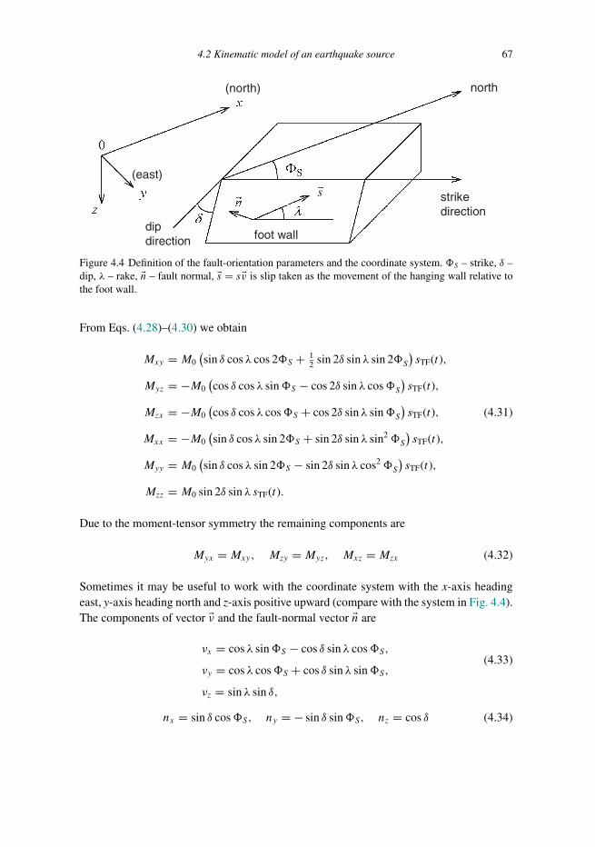
Trim: 247mm × 174mm Top: 14.762mm Gutter: 23.198mmCUUK2497-04 CUUK2497/Moczo ISBN: 978 1 107 02881 4 November 14, 2013 20:31
4.2 Kinematic model of an earthquake source 67
s
foot walldipdirection
strikedirection
(north)
(east)
north
Figure 4.4 Definition of the fault-orientation parameters and the coordinate system. �S – strike, δ –dip, λ – rake, �n – fault normal, �s = s�v is slip taken as the movement of the hanging wall relative tothe foot wall.
From Eqs. (4.28)–(4.30) we obtain
Mxy = M0(sin δ cos λ cos 2�S + 1
2 sin 2δ sin λ sin 2�S)sTF(t),
Myz = −M0(cos δ cos λ sin�S − cos 2δ sin λ cos�S
)sTF(t),
Mzx = −M0(cos δ cos λ cos�S + cos 2δ sin λ sin�S
)sTF(t), (4.31)
Mxx = −M0(sin δ cos λ sin 2�S + sin 2δ sin λ sin2�S
)sTF(t),
Myy = M0(sin δ cos λ sin 2�S − sin 2δ sin λ cos2�S
)sTF(t),
Mzz = M0 sin 2δ sin λ sTF(t).
Due to the moment-tensor symmetry the remaining components are
Myx = Mxy, Mzy = Myz, Mxz = Mzx (4.32)
Sometimes it may be useful to work with the coordinate system with the x-axis headingeast, y-axis heading north and z-axis positive upward (compare with the system in Fig. 4.4).The components of vector �ν and the fault-normal vector �n are
νx = cos λ sin�S − cos δ sin λ cos�S,
νy = cos λ cos�S + cos δ sin λ sin�S,
νz = sin λ sin δ,
(4.33)
nx = sin δ cos�S, ny = − sin δ sin�S, nz = cos δ (4.34)

Trim: 247mm × 174mm Top: 14.762mm Gutter: 23.198mmCUUK2497-04 CUUK2497/Moczo ISBN: 978 1 107 02881 4 November 14, 2013 20:31
68 Earthquake source
From Eqs. (4.28), (4.33) and (4.34) we obtain
Mxy = M0(sin δ cos λ cos 2�S + 1
2 sin 2δ sin λ sin 2�S)sTF(t),
Myz = M0(cos δ cos λ cos�S + cos 2δ sin λ sin�S
)sTF(t),
Mzx = M0(cos δ cos λ sin�S − cos 2δ sin λ cos�S
)sTF(t),
Mxx = M0(sin δ cos λ sin 2�S − sin 2δ sin λ cos2�S
)sTF(t),
Myy = −M0(sin δ cos λ sin 2�S + sin 2δ sin λ sin2�S
)sTF(t),
Mzz = M0 sin 2δ sin λ sTF(t).
(4.35)
4.2.2 Finite-fault kinematic source
In situations when we are interested in the wavefield at distances comparable to or smallerthan the size of the fault, the point-source approximation is not appropriate. In such situa-tions we have to consider the finite-fault source. If using the dynamic source is not feasible,we may use the finite-fault kinematic source.
Recall the representation theorem (4.16),
un(�x, t) =∫ ∞
−∞dτ
∫S
mpq(�ξ, τ )∂Gnp(�x, t − τ ; �ξ, 0)
∂ξqdS (4.36)
Divide the fault surface S into k nonoverlapping sub-faults Sk . Then,
un(�x, t) =∑k
(∫Sk
mpq ∗ ∂Gnp∂ξq
dS
)(4.37)
Consider each sub-fault as a point source. Consequently, we consider one Green tensor persub-fault. Then,
un(�x, t) =∑k
(∫Sk
mpqdS ∗ ∂Gknp
∂ξq
)=∑k
(Mkpq ∗ ∂G
knp
∂ξq
)(4.38)
Assuming only tangential slip on each sub-fault we can use Eqs. (4.21)–(4.23) to expressthe moment-tensor components for sub-faults:
Mkpq = μk
(nkpν
kq + nkqνkp
) ∫Sk
sdS (4.39)
Similarly as in the case of a point source the integral can be approximated using Eq. (4.24):
Mkpq = μk sk skTF(t)Ak
(nkpν
kq + nkqνkp
). (4.40)
Here Ak is size of the k-th sub-fault surface and skTF(t) is the source-time function for thek-th sub-fault:
skTF(t) ≡ sk(t)
sk, sk ≡ sk (t → ∞) (4.41)

Trim: 247mm × 174mm Top: 14.762mm Gutter: 23.198mmCUUK2497-04 CUUK2497/Moczo ISBN: 978 1 107 02881 4 November 14, 2013 20:31
4.2 Kinematic model of an earthquake source 69
Using the scalar moment we can write
Mkpq = Mk
0
(nkpν
kq + nkqνkp
)skTF(t) (4.42)
In this derivation we considered the point-source assumptions for each sub-fault. Therefore,the finite-fault kinematic source is represented by a set of point sources. Each point source ischaracterized by its position �xk and moment-tensor componentsMk
pq (including the source-time functions skTF(t) ). We can also characterize each point source by strike �kS , dip δk ,rake λk , scalar momentMk
0 and source-time function skTF(t), and use Eqs. (4.31) or (4.35) toobtain the moment-tensor components. Note that a source-time function (4.41) is definedfor each point source since rupture nucleated at a hypocentre. For a single point sourcethis is natural. In the case of finite-fault kinematic models, usually source-time functionand rupture-onset time are defined for each point source. Rupture-onset time defines whenrupture arrives at a particular point and after that time the time evolution is prescribed bythe source-time function. In this way the rupture propagation is controlled by rupture onsettime and the source-time functions are defined only for the time they are really needed.

Trim: 247mm × 174mm Top: 14.762mm Gutter: 23.198mmCUUK2497-04 CUUK2497/Moczo ISBN: 978 1 107 02881 4 November 14, 2013 20:31

Trim: 247mm × 174mm Top: 14.762mm Gutter: 23.198mmCUUK2497-05 CUUK2497/Moczo ISBN: 978 1 107 02881 4 November 14, 2013 21:14
Part IIThe finite-difference method

Trim: 247mm × 174mm Top: 14.762mm Gutter: 23.198mmCUUK2497-05 CUUK2497/Moczo ISBN: 978 1 107 02881 4 November 14, 2013 21:14

Trim: 247mm × 174mm Top: 14.762mm Gutter: 23.198mmCUUK2497-05 CUUK2497/Moczo ISBN: 978 1 107 02881 4 November 14, 2013 21:14
5
Time-domain numerical methods
5.1 Introduction
A large variety of time-domain methods have been developed for modelling earthquakeground motion. They may be divided into three groups – boundary methods, domainmethods and hybrid methods (note that the adjectives boundary and domain here relateto space). In general, the boundary methods are more accurate than the domain methods,but they are not computationally efficient in the case of complex (realistic) models. Thereasonable balance of accuracy and computational efficiency in applications to complexmodels is the primary reason why the domain methods are dominant, not only in therecent modelling of earthquake motion but also in waveform inversion. Development ofhybrid approaches is the consequence of a simple but important fact – no single method isthe most accurate and computationally efficient for all wavefield–medium configurations.Combining two or more methods makes it possible to overcome the limitations of individualmethods.
In this book we do not address the boundary methods. For an excellent overview ofthe boundary integral equation, boundary-element, discrete-wavenumber and Aki–Larnermethods as well as of the hybrid approaches we refer to Bouchon and Sanchez-Sesma(2007).
The finite-difference method (FDM), finite-element method (FEM), Fourier pseudo-spectral method (FPSM), spectral-element method (SEM), and discontinuous Galerkinmethod (DGM) are the most representative domain methods for modelling rupture prop-agation, seismic wave propagation and earthquake ground motion. The domain methodsprimarily differ from each other by their approach to spatial discretization. In this book weaddress in detail FDM or, more precisely, FDTD (finite-difference time-domain) method,and briefly FEM and their hybrid combination. Therefore, we include in the next threesections of this chapter concise descriptions of FPSM, SEM and ADER-DGM contributedby Peter Klin, Emmanuel Chaljub, Martin Kaser and Christian Pelties.
The three following sections and the subsequent chapters refer to many important arti-cles related to the methods. Here we just mention books and chapters in books that provideintroductions and overviews of the numerical domain methods: Chaljub et al. (2007) forSEM, de la Puente (2008) for ADER-DGM, Moczo et al. (2007a,b) for FDM. We may
73
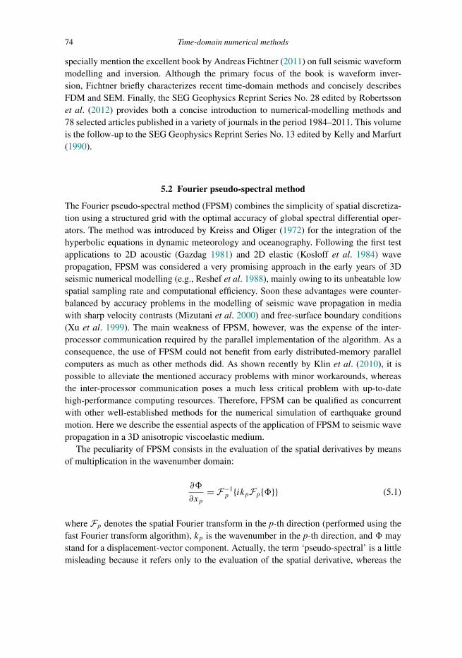
Trim: 247mm × 174mm Top: 14.762mm Gutter: 23.198mmCUUK2497-05 CUUK2497/Moczo ISBN: 978 1 107 02881 4 November 14, 2013 21:14
74 Time-domain numerical methods
specially mention the excellent book by Andreas Fichtner (2011) on full seismic waveformmodelling and inversion. Although the primary focus of the book is waveform inver-sion, Fichtner briefly characterizes recent time-domain methods and concisely describesFDM and SEM. Finally, the SEG Geophysics Reprint Series No. 28 edited by Robertssonet al. (2012) provides both a concise introduction to numerical-modelling methods and78 selected articles published in a variety of journals in the period 1984–2011. This volumeis the follow-up to the SEG Geophysics Reprint Series No. 13 edited by Kelly and Marfurt(1990).
5.2 Fourier pseudo-spectral method
The Fourier pseudo-spectral method (FPSM) combines the simplicity of spatial discretiza-tion using a structured grid with the optimal accuracy of global spectral differential oper-ators. The method was introduced by Kreiss and Oliger (1972) for the integration of thehyperbolic equations in dynamic meteorology and oceanography. Following the first testapplications to 2D acoustic (Gazdag 1981) and 2D elastic (Kosloff et al. 1984) wavepropagation, FPSM was considered a very promising approach in the early years of 3Dseismic numerical modelling (e.g., Reshef et al. 1988), mainly owing to its unbeatable lowspatial sampling rate and computational efficiency. Soon these advantages were counter-balanced by accuracy problems in the modelling of seismic wave propagation in mediawith sharp velocity contrasts (Mizutani et al. 2000) and free-surface boundary conditions(Xu et al. 1999). The main weakness of FPSM, however, was the expense of the inter-processor communication required by the parallel implementation of the algorithm. As aconsequence, the use of FPSM could not benefit from early distributed-memory parallelcomputers as much as other methods did. As shown recently by Klin et al. (2010), it ispossible to alleviate the mentioned accuracy problems with minor workarounds, whereasthe inter-processor communication poses a much less critical problem with up-to-datehigh-performance computing resources. Therefore, FPSM can be qualified as concurrentwith other well-established methods for the numerical simulation of earthquake groundmotion. Here we describe the essential aspects of the application of FPSM to seismic wavepropagation in a 3D anisotropic viscoelastic medium.
The peculiarity of FPSM consists in the evaluation of the spatial derivatives by meansof multiplication in the wavenumber domain:
∂�
∂xp= F−1
p {ikpFp{�}} (5.1)
where Fp denotes the spatial Fourier transform in the p-th direction (performed using thefast Fourier transform algorithm), kp is the wavenumber in the p-th direction, and � maystand for a displacement-vector component. Actually, the term ‘pseudo-spectral’ is a littlemisleading because it refers only to the evaluation of the spatial derivative, whereas the

Trim: 247mm × 174mm Top: 14.762mm Gutter: 23.198mmCUUK2497-05 CUUK2497/Moczo ISBN: 978 1 107 02881 4 November 14, 2013 21:14
5.2 Fourier pseudo-spectral method 75
temporal evolution is usually solved using nonspectral approaches. The usual choice is the2nd-order explicit FD scheme:
�u (�x, t +�t) = 2�u (�x, t) − �u (�x, t −�t) + (�t)2 ∂2 �u (�x, t)∂t2
(5.2)
where �u is the displacement vector. The equation of motion for a viscoelastic anisotropicmedium can be expressed as
∂2 �u (�x, t)∂t2
= 1
ρ (�x)∇ · [C (�x) ∇T �u (�x, t) + R (�x, t)]+ �f (�x, t) (5.3)
where C is the 6 × 6 symmetric elasticity matrix (in Voigt notation), R is the 6-componentvector that accounts for viscoelasticity, �f is the source term, and ∇ is the spatial differen-tiation operator:
∇ =⎛⎝∂x 0 0 0 ∂z ∂y
0 ∂y 0 ∂z 0 ∂x0 0 ∂z ∂y ∂x 0
⎞⎠ (5.4)
Viscoelasticity and attenuation correspond to the rheology of the generalized Maxwellbody (GMB-EK in Chapter 3) and the term R includes the anelastic functions (memoryvariables).
The differentiation approach described in Eq. (5.1) is exact if the amplitude spectrum ofthe wavefield vanishes for wavenumbers larger than the Nyquist wavenumber kN = π/h,where h is the grid spacing. Therefore FPSM allows for a relatively coarse spatial sampling(Fornberg 1987), which represents a valuable advantage in solving 3D problems. On theother hand, the nature of the global differential operators implies that numerical artefactsare spread over the whole spatial domain when a singularity arises in the wavefield (Gibb’sphenomenon). This problem is significantly reduced if the differential operators are definedon staggered grids (Ozdenvar and McMechan 1996) and formally expressed as
D±p � = F−1
p
{ikp exp
(±ikp 12h)Fp {�}} (5.5)
Operators D+p and D−
p evaluate the spatial derivative of � in the grid (the staggered grid)which is shifted by h/2 in the p-th direction, forward and backward, respectively. In orderto obtain the acceleration terms in the same grid, where the displacement terms are defined,the application of operators D+
p and D−p should follow an adequate inter-changing role
while solving the equation of motion.In earthquake ground motion simulations the free-surface boundary condition is typically
imposed on the top of the spatial domain. The condition implies discontinuities in theperiodic extension of the differentiated wavefield, which in turn appears ill-suited forthe operators defined in Eq. (5.5). In order to incorporate the free-surface condition, thedifferentiated wavefield is first appropriately modified – it has to be made suitable forapplication of the differential operator. Once the operator is applied, the known effects of theemployed modification are removed. The modification consists in the removal of possiblediscontinuities in the displacement field across points at which the free-surface condition

Trim: 247mm × 174mm Top: 14.762mm Gutter: 23.198mmCUUK2497-05 CUUK2497/Moczo ISBN: 978 1 107 02881 4 November 14, 2013 21:14
76 Time-domain numerical methods
is imposed by means of subtraction of a linear function evaluated from the discontinuity.In order to account for the modification, a sum of constant value is applied to the obtainedderivative. The free-surface condition is imposed using stress imaging (Subsection 10.1.1),but the same result can be obtained by using a sine transform instead of the ordinary fastFourier transform to transform the stress field in the wavenumber domain and by returningwith the cosine transform after the wavenumber multiplication.
FPSM is based on the heterogeneous formulation of the equation of motion. In con-sequence, the use of a relatively coarse regular spatial sampling exposes it particularly tonumerical artefacts caused by staircase approximations of nonplanar material interfaces.The approaches based on mapping of the computational grid to the geometry of the maininterfaces (e.g., Fornberg 1988b), which were proposed to mitigate these artefacts, appearimpractical in the general 3D case. More workable approaches consist in honouring thediscretization rules proposed by Pelties et al. (2010), and in adopting the volume harmonicaveraging of the elastic moduli and volume arithmetic averaging of density proposed byMoczo et al. (2002) for the FD modelling schemes. The homogenization approach (e.g.,Capdeville and Marigo 2007, 2013, Capdeville et al. 2010a,b, 2013) seems to be a reason-able perspective.
The rectangular spatial grid makes it easy to implement PML (Chapter 12) in order tosimulate absorbing boundary conditions for the outgoing wavefield at boundaries of thespatial grid.
FPSM can be successfully applied in the numerical simulation of the seismic wavefieldproduced by an earthquake in large 3D crustal models (Vuan et al. 2011). We refer to Klinet al. (2010) for a more comprehensive review of FPSM and related discussions.
5.3 Spectral element method
The spectral element method (SEM) was developed in the eighties in the field of computa-tional fluid dynamics (Patera 1984, Maday and Patera 1989) with the objective to extendthe spectral method to deal with realistic 2D or 3D geometries, to capture local variationsof the physical solutions and to alleviate implementation of boundary conditions.
For example, in the spectral method, complex geometries can only be handled by theso-called ‘mapping and patching’ strategy (Boyd 2001): a computational domain is firstsplit into regions, or sub-domains, each of which is the image of a canonical domain (e.g.,a cube in 3D) through a regular mapping. The solutions on each sub-domain are expandedon a local spectral basis (trigonometric functions or orthogonal polynomials), then patchedtogether by enforcing the continuity of the displacement and traction vectors, usuallythrough iterative procedures and/or overlapping strategies. For complex geometries, thereis a trade-off between increasing the number of sub-domains to accurately represent thegeometry of the domain and solving the resulting system of interface conditions. Moreover,this domain decomposition strategy does not change the fact that boundary conditions haveto be enforced with special care and usually leads to lower accuracy near the boundariesaffecting, e.g., surface waves.

Trim: 247mm × 174mm Top: 14.762mm Gutter: 23.198mmCUUK2497-05 CUUK2497/Moczo ISBN: 978 1 107 02881 4 November 14, 2013 21:14
5.3 Spectral element method 77
As stated by Komatitsch and Vilotte (1998), SEM could have developed after the simi-larity between the spectral collocation methods (in which the equation of motion is exactlysatisfied by the numerical solution at some well-chosen points) and variational formulationswith consistent quadrature (numerical integration formula) was understood.
Thus, SEM relies on the variational formulation (weak form) of the equation of motionand in most cases its displacement formulation, in which the displacement field is forcedto be globally continuous whereas the continuity of the traction vector (also at the freesurface) is satisfied implicitly. We refer to Cohen and Fauqueux (2005) for the mixedvelocity–stress formulation and to Festa and Vilotte (2005) for a comparative analysis ofthe two formulations. Here we just note that the mixed formulation makes it easier toimplement PML.
SEM appears as an FEM where the solution is expanded in each element onto spectralpolynomial bases of high order and where numerical integration is realized with Gauss–Jacobi quadratures. It is therefore connected to the h− p version of FEM, where theaccuracy of the numerical solution can be increased by decreasing the element size h or byincreasing the local polynomial order p.
The first applications of SEM to acoustic and elastic wave propagation by Serianiand Priolo (1994) and Priolo et al. (1994) used Chebyshev polynomials together withGauss–Lobatto–Chebyshev quadrature – as Patera (1984) did in his original article. Theimplementation combined the geometrical flexibility of FEM with the accuracy of thespectral methods and minimized numerical dispersion and dissipation even in challengingapplications involving interface and surface waves. One drawback was that the mass matrixhad to be inverted when an FD scheme was used for time evolution. This problem wascircumvented independently by Faccioli et al. (1997) and by Komatitsch and Vilotte (1998):they used Gauss–Lobatto–Legendre quadrature together with polynomial bases built uponLegendre polynomials to derive SEM in which the mass matrix is diagonal (as in the articleof Maday and Patera 1989). The implementation has become most popular in seismicapplications for its computational efficiency, resulting from the use of the explicit FDtime-evolution schemes, without any loss of accuracy compared to the use of Chebyshevpolynomials and quadrature.
In all the above SEM implementations (Chebyshev or Legendre type), the polynomialbases are first built in one space dimension, then extrapolated by tensorization to 2D and 3D.This represents a gain in computational efficiency but also a constraint that the geometry ofthe elements has to be tensorized too: the elements are restricted to deformed quadrilateralsin 2D and hexahedra in 3D. The problem of finding an accurate quadrature that wouldpossibly preserve the diagonality of the mass matrix for non-tensorized geometries is stillopen – as discussed by Mercerat et al. (2006), who implemented SEM for 2D triangulargrids.
The optimal choice of the polynomial order for SEM is between N = 4 and N = 8:the lower orders do not significantly reduce numerical dispersion whereas higher ordersresult in a too severe Courant–Friedrichs–Lewy condition for the time step, which is notcompensated by the number of grid points per wavelength needed for an acceptable level of

Trim: 247mm × 174mm Top: 14.762mm Gutter: 23.198mmCUUK2497-05 CUUK2497/Moczo ISBN: 978 1 107 02881 4 November 14, 2013 21:14
78 Time-domain numerical methods
numerical dispersion and anisotropy (Seriani and Oliveira 2007, de Basabe and Sen 2007).An average number of five or six grid points per wavelength (i.e., about one element ifN = 4 and half an element if N = 8 ) is used in practical applications.
Surprisingly, choosing an appropriate h can be a much more difficult task when dealingwith complex heterogeneous 3D models. The main problem is how to represent variationsof geometrical or mechanical properties that occur on scales smaller than the minimumpropagating wavelength. A material discontinuity is a very good example. The polynomialbases used in SEM are not adapted to represent such variations – as in the original SM.The only possibility is to have the discontinuity coincide with the boundaries of elements.This approach can, however, pose a tremendous meshing task in some applications – seeChaljub et al. (2010). In such cases, the so-called homogenization (e.g., Capdeville andMarigo 2007, 2013, Capdeville et al. 2010a,b, 2013) can probably help.
For reviews presenting the numerous developments of the Legendre SEM for global orregional seismology applications we refer to Komatitsch et al. (2005) and Chaljub et al.(2007). For examples of earthquake ground motion simulations including effects of localgeology we refer to Komatitsch et al. (2004), Lee et al. (2008b, 2009), Stupazzini et al.(2009a,b), Chaljub et al. (2010), Pilz et al. (2011). SEM has also been applied to studyrupture dynamics; e.g., Madariaga et al. (2006), Festa and Vilotte (2006), Kaneko et al.(2008, 2011). Computational aspects can be found in articles by Komatitsch et al. (2010)and Peter et al. (2011).
Here, we briefly recall the key features of the Legendre SEM discretization. We recallthe weak form of the equation of motion, Eq. (2.12), which can be rewritten as
∂2
∂t2
∫�
ρ �u · �wd�+∫�
σij (�u) εij ( �w) d� =∫�
�T · �wd� +∫�
�f · �wd� (5.6)
where� is the computational domain and � its boundary with prescribed traction �T . Otherquantities are the same as those in Eq. (2.12).
The spatial discretization starts with a decomposition of the computational domain �intoK unstructured non-overlapping hexahedral elements�k; k = 1, . . . , K . Each elementis obtained by a regular mapping of a reference element �ref (the unit cube in 3D). Then,virtual (also admissible) displacements are approximated by polynomials of degree N ineach element and we obtain
K∑k=1
∂2
∂t2
∫�k
ρ �ujN · �wjNd�+K∑k=1
∫�kσln
(�ujN)εln
(�wjN)d�
=K∑k=1
∫�k
�T jN · �wjNd� +K∑k=1
∫�k
�f jN · �wjN d�; j = 1, . . . , N
(5.7)
where �ujN , �wjN , �T jN and �f jN are scalar j-th components of vectors approximating �u, �w, �Tand �f , respectively. The summation convention is assumed for indices j, l, n, and is notassumed for indexN . Note that in Eq. (5.7) we implicitly assume that the displacements are
Trim: 247mm × 174mm Top: 14.762mm Gutter: 23.198mmCUUK2497-05 CUUK2497/Moczo ISBN: 978 1 107 02881 4 November 14, 2013 21:14
5.4 ADER spectral discontinuous Galerkin scheme 79
continuous but the material properties can be discontinuous across elements. The integralsin Eq. (5.7) are evaluated numerically by a high-order quadrature based on the Gauss–Lobatto–Legendre (GLL) points and weights (e.g., Canuto et al. 1988). The polynomialsused for approximating the displacements are then defined as the Lagrange interpolants ofthe GLL points. Assembling the elementary contributions to account for the continuity ofdisplacements, Eq. (5.7) can be written as a global system of ordinary differential equationsin time:
M U (t) + KU (t) = F (t) + T (t) (5.8)
where F(t) and T(t) are global vectors accounting for external body force and tractions,respectively, M and K are global mass and stiffness matrices, respectively, and U (t) isthe global vector of discrete (approximating) displacements. An important consequenceof the choice of the polynomial basis is that the mass matrix is diagonal, which, as statedpreviously, allows for the use of a fully explicit FD scheme for the time evolution. Thelatter is usually done using the explicit, conditionally stable, 2nd-order leapfrog scheme(e.g., Maggio and Quarteroni 1994).
5.4 Spectral discontinuous Galerkin scheme with ADER time integration
The discontinuous Galerkin (DG) FE scheme combined with a time integration techniqueusing Arbitrarily high order DERivatives (ADER) is a numerical method for solving the 3Dequations of motion in the velocity–stress formulation. A hyperbolic system of equationsmay be concisely written for isotropic or anisotropic elastic, viscoelastic or poroelasticmedia in the form (see Eq. (2.33)),
∂Qp
∂t+ Apq ∂Qq
∂ξ+ Bpq ∂Qq
∂η+ Cpq ∂Qq
∂ζ= EpqQq + Sp (5.9)
Here
Q = (σxx, σyy, σzz, σxy, σyz, σxz, vx, vy, vz)T (5.10)
The Jacobian matrices Apq , Bpq and Cpq include parameters corresponding to the typeof medium (Dumbser and Kaser 2006, Kaser et al. 2007, de la Puente et al. 2007, 2008).Matrix Epq represents viscoelasticity and attenuation corresponding to the rheology of thegeneralized Maxwell body (GMB-EK in Chapter 3). Term Sp is an external source termrepresenting forces of the moment-tensor sources.
In the DG approach the solution is approximated inside each tetrahedral element bya linear combination of space-dependent polynomial basis functions and time-dependentdegrees of freedom, as expressed through
(Qh)p(ξ, η, ζ, t) = Qpl(t)�l(ξ, η, ζ ) (5.11)
where the basis functions �l form an orthogonal modal basis and are defined on thecanonical reference tetrahedron such that no integration points are necessary. For a detailed

Trim: 247mm × 174mm Top: 14.762mm Gutter: 23.198mmCUUK2497-05 CUUK2497/Moczo ISBN: 978 1 107 02881 4 November 14, 2013 21:14
80 Time-domain numerical methods
derivation of the numerical scheme we refer to articles by Kaser and Dumbser (2006),and Dumbser and Kaser (2006). The unique property of the ADER-DG scheme is thatthe temporal accuracy of the scheme is automatically coupled to the spatial accuracydetermined by the degree of approximation polynomials used in Eq. (5.11). This is dueto the ADER time-integration approach (Titarev and Toro 2002) that uses a Taylor seriesexpansion in time of the solution of Eq. (5.9), replacing all temporal derivatives recursivelyby spatial derivatives. Thus, the Taylor series expansion only depends on spatial derivativesof the basis functions and lower-order time derivatives of the source terms. The resultingexpression for the degrees of freedom can be integrated in time analytically as shown indetail by Dumbser and Kaser (2006) or Kaser et al. (2007). Therefore, the ADER-DGapproach provides an arbitrarily high order approximation in space and time depending onthe degree of the used basis polynomials in Eq. (5.11) and the corresponding order of thechosen Taylor series in time.
Once the high-order time-integrated degrees of freedom are computed, the evolution ofthe numerical solution in time is calculated via local stiffness and flux terms (Dumbser andKaser 2006). Numerical fluxes out of an element and into an element have to be calculatedfor each element boundary, i.e., triangular surface, for each tetrahedral element. Each fluxcomputation requires a multiplication of two dense matrices with dimensions (N ×N ) and(N × 9), respectively, with N being the number of degrees of freedom and 9 the numberof variables in the vector of unknowns in Eq. (5.10). The calculation of the three stiffnessterms has to be carried out only once per element via a multiplication of two matricesof the same size as above; however, the (N ×N ) stiffness matrix is typically sparse. Alloperations use only local data from the element itself and its direct neighbour elementsharing a common boundary. Due to this local character of the numerical scheme it is wellsuited for parallel computing.
With the ADER-DG approach it is possible to vary the degree of the approximationpolynomials in Eq. (5.11) from one element to another. Due to the direct coupling of thetemporal and spatial accuracy via the ADER approach, the scheme automatically becomesadaptive in temporal accuracy – this is the so-called pτ -adaptation. The pτ -adaptationallows for an adaptive choice of spatial accuracy, which enhances computational efficiencyin most applications. This is because the computational domain is typically larger than theparticular zone of interest where high-order accuracy is required. Even more important, theADER-DG method can use local time stepping to reduce computational cost. Geometricallycomplex computational domains or requirements on spatial resolution often lead to meshesincluding small and large elements with significant differences in the element size. Thetime step for the explicit numerical schemes is restricted by the ratio of the mesh sizeh of the smallest element and the corresponding maximum wave speed in this element.For the global time-stepping schemes all elements are updated with this possibly stronglyrestrictive time step. This can lead to a large number of time levels that must be computed.With the ADER approach, time-accurate local time stepping can be used: each elementcan be updated with its own optimal time step. An element can be updated to the nexttime level if its actual time level and its local time step fulfil a certain update criterion.

Trim: 247mm × 174mm Top: 14.762mm Gutter: 23.198mmCUUK2497-05 CUUK2497/Moczo ISBN: 978 1 107 02881 4 November 14, 2013 21:14
5.5 Hybrid methods 81
The information exchange between elements across their joint boundaries works throughnumerical fluxes that depend on the length of the local time interval over which the fluxis integrated. The local time-stepping approach can reduce the overall amount of fluxcalculations dramatically because only the small elements have to be updated frequentlyaccording to their small time steps. For a complete description of the pτ -adaptation andlocal time stepping see the article by Dumbser et al. (2007).
De la Puente et al. (2009) and Pelties et al. (2012) demonstrated that the ADER-DGmethod is capable of numerically simulating dynamic rupture propagation on complexfaults without spurious high-frequency oscillations, which pose a serious problem forother numerical grid methods. The latter aspect is important for earthquake source studiesas well as for numerical simulation of earthquake ground motion. Moreover, the pτ -adaptation and local time stepping can be advantageous in the cohesive zone of frictionalsliding.
The absence of the spurious high-frequency oscillations is due to the numerical prop-erties of the exact Riemann solver (Godunov flux). In fact, the constitutive friction lawis incorporated in the solution of the so-called inverse Riemann problem at element inter-faces. A mesh is constructed so that the fault everywhere coincides with the interface of twoelements. The Godunov flux is an upwind scheme that is intrinsically dissipative, with theattribute that the dissipation increases steeply as a function of frequency depending on theelement size and applied order of approximation. Therefore, the high-frequency content isadaptively damped without perturbing the lower, physically meaningful frequencies. Actu-ally, this numerical property has two positive consequences: (1) no spurious high-frequencyoscillations during frictional sliding, (2) mesh coarsening (h-adaptivity) is possible withoutcausing artificial reflections or instabilities at the area of grid refinement due to numericalimpedance.
The method has been successfully applied also to more advanced dynamic ruptureproblems such as bi-material faults, faults with heterogeneous stress loading, surface rup-ture, and fault branching (see SCEC Dynamic Rupture Code Verification Project: http://scecdata.usc.edu/cvws/). The method can accommodate both the linear slip-weakening andrate-and-state type friction laws.
The discontinuous Galerkin method is a powerful general approach that can be the basisfor a variety of formulations. We refer to, e.g., de Basabe et al. (2008), Delcourte et al.(2009), Etienne et al. (2010), Wilcox et al. (2010) and Tago et al. (2012).
5.5 Hybrid methods
Each of the many computational and numerical methods that have been developed so far forseismic wave propagation and earthquake motion has at least one feature in which it is betteror more advantageous compared to other methods – at least with respect to some specificmedium–wavefield configuration. On the other hand, none of the existing methods can beconsidered the most accurate and, at the same time, the most computationally efficientfor all important medium–wavefield configurations. In many problem configurations it is

Trim: 247mm × 174mm Top: 14.762mm Gutter: 23.198mmCUUK2497-05 CUUK2497/Moczo ISBN: 978 1 107 02881 4 November 14, 2013 21:14
82 Time-domain numerical methods
therefore reasonable to combine two or even more computational methods in order to solvethe problem with a reasonable level of accuracy and computational efficiency.
It can be advantageous to solve the time dependence of a field variable using onemethod and the spatial dependence using some other method. For example, Alexeevand Mikhailenko (1980) combined partial separation of variables and an FD method,Mikhailenko and Korneev (1984) combined the finite integral Fourier transform and FDM.
It can be advantageous to split the computational domain into two or more parts andsolve each part by the best-suited method. For example, one method may be applied in asub-domain that includes a dynamically rupturing fault, another method may be applied inthe sub-domain that includes topography of the free surface, and one method may be appliedin the major part of the whole computational domain for efficient seismic wave propagation.Another example is the configuration in which we are interested in detailed modelling ofearthquake ground motion in a surface local structure due to a relatively distant source. Inthis type of hybrid approach it is important to develop a stable and noise-free algorithm,ensuring the causal communication between neighbouring sub-domains respecting thephysics of the adopted model. Several hybrid methods have been developed, most ofthem in 2D, in an effort to achieve reasonable computational efficiency in applications torelatively complex structural models. They include methods by Ohtsuki and Harumi (1983),Shtivelman (1984, 1985), Van den Berg (1984), Kummer et al. (1987), Kawase (1988),Stead and Helmberger (1988), Emmerich (1989, 1992), Gaffet and Bouchon (1989), Fah(1992), Fah et al. (1993), Bouchon and Coutant (1994), Rovelli et al. (1994), Robertssonet al. (1996), Zahradnık and Moczo (1996), Moczo et al. (1997), Lecomte et al. (2004), Maet al. (2004), Galis et al. (2008), Zhao et al. (2008), Liu and Sen (2010), Liu et al. (2011),Monteiller et al. (2012). Extensive references on the hybrid approaches can be found in thearticle by Oprsal et al. (2009).
In Chapter 18 we describe the hybrid FD–FE method developed by Galis et al. (2008).

Trim: 247mm × 174mm Top: 14.762mm Gutter: 23.198mmCUUK2497-06 CUUK2497/Moczo ISBN: 978 1 107 02881 4 November 15, 2013 13:32
6
Brief introduction to the finite-difference method
Application of the method to a particular differential problem includes:
(a) Construction of a discrete FD model of the problem:– coverage of the computational domain by a space–time grid,– FD approximations of derivatives, functions, initial and/or boundary condition at the
grid points,– construction of a system of algebraic equations; we may call them FD equations or
FD scheme.(b) Analysis of the FD model
– consistency and order of the approximation,– stability and grid dispersion,– convergence,– local error.
(c) Numerical computations.
Analysis of the FD model and numerical computations may lead to redefinition of the gridand FD approximations if the numerical behaviour of the developed FD scheme is notsatisfactory.
Note that in the case of the so-called explicit FD schemes (see later), the term ‘scheme’is often used in a narrower meaning for the explicit algebraic formula for updating a fieldvariable (displacement or particle-velocity or stress-tensor component) at a spatial gridposition.
6.1 Space–time grids
6.1.1 Cartesian grid
Consider a spatial Cartesian coordinate system (x, y, z) and a computational domain in the4D space of variables (x, y, z, t) with t meaning time. A set of discrete space–time points(or positions)
(xI , yK, zL, tm), I,K,L,m ∈ {0, 1, 2, . . .}xI = x0 + I�xI , yK = y0 +K�yK, zL = z0 + L�zL, tm = t0 +m� (6.1)
83

Trim: 247mm × 174mm Top: 14.762mm Gutter: 23.198mmCUUK2497-06 CUUK2497/Moczo ISBN: 978 1 107 02881 4 November 15, 2013 13:32
84 Brief introduction to the finite-difference method
defines a space–time grid. Grid coordinates xI , yK, zL determine a spatial grid point (posi-tion), coordinate tm determines a time level. The spatial increments�xI ,�yK and�zL areusually called grid spacings, � is the time step. The value of a function ϕ at the grid point(xI , yK, zL, tm), that is ϕ (xI , yK, zL, tm), may be denoted by ϕ (I,K,L,m) or ϕmI,K,L orϕ|mI,K,L. The exact value should be distinguished from its FD approximation, which maybe denoted, e.g., by �mI,K,L.
The Cartesian coordinate system is convenient and natural for modelling of earthquakemotion in local surface structures. Systems other than Cartesian coordinate systems can bealso used to define a grid. The particular choice should be problem dependent. Whereasspherical coordinates might be convenient for whole Earth models, cylindrical coordinatesmight be more suitable for borehole modelling. The choice of the grid determines thestructure and properties of the FD approximations of derivatives, and consequently theproperties of the FD scheme.
6.1.2 Uniform, nonuniform and discontinuous grids
A grid specified by Eqs. (6.1) is nonuniform in all coordinate directions – the size of thegrid spacing in general varies point to point. In many applications it might be reasonableto use �xI = �yK = �zL = h. In such a case the grid is uniform. The use of a uniformgrid usually yields the algorithmically simplest FD schemes. This, however, may contradictthe computational efficiency. Therefore, in some applications it is advantageous to use aspatially discontinuous grid – part of the computational domain is covered with a uniformgrid with grid spacing hF whereas the rest of the computational domain is covered with auniform grid with grid spacing hC > hF . The subscripts indicate coarser and finer grids,respectively. This is usually related to the heterogeneity of the medium. It is also possibleto use a grid that is discontinuous in size of spatial grid spacing and/or time step.
6.1.3 Structured and unstructured grids
If at a grid point explicit information about the connection to neighbouring grid points isneeded we speak about unstructured grids. If at a grid point explicit information is notneeded (e.g., we can find neighbouring grid points just by using indices) we speak aboutstructured grids. Obviously, structured grids usually yield computationally faster algorithmscompared to those on unstructured grids.
6.1.4 Space–time locations of field variables
Grids and consequently FD schemes may differ in the grid positions of thedisplacement/particle-velocity and stress-tensor components. It is natural to think of havingall of them at each space–time grid position. Clearly, such location of all field variables isideal for imposing initial and boundary conditions in an isotropic medium and, in general,for an anisotropic medium. As will be seen later, however, having all field variables at
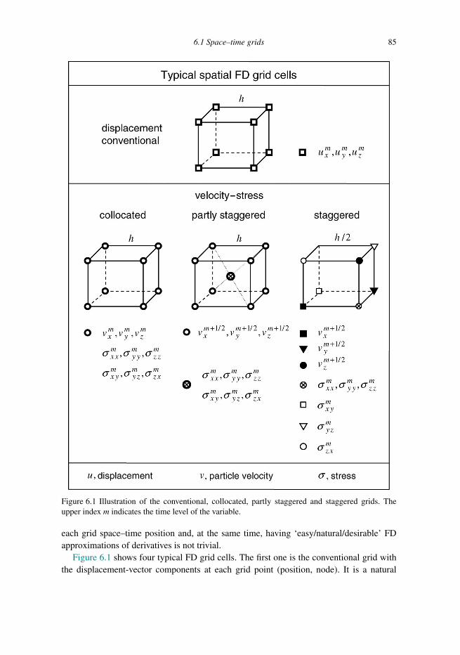
Trim: 247mm × 174mm Top: 14.762mm Gutter: 23.198mmCUUK2497-06 CUUK2497/Moczo ISBN: 978 1 107 02881 4 November 15, 2013 13:32
6.1 Space–time grids 85
Figure 6.1 Illustration of the conventional, collocated, partly staggered and staggered grids. Theupper index m indicates the time level of the variable.
each grid space–time position and, at the same time, having ‘easy/natural/desirable’ FDapproximations of derivatives is not trivial.
Figure 6.1 shows four typical FD grid cells. The first one is the conventional grid withthe displacement-vector components at each grid point (position, node). It is a natural

Trim: 247mm × 174mm Top: 14.762mm Gutter: 23.198mmCUUK2497-06 CUUK2497/Moczo ISBN: 978 1 107 02881 4 November 15, 2013 13:32
86 Brief introduction to the finite-difference method
grid for displacement schemes solving the displacement formulation of the equation ofmotion (the 2nd-order equation of motion). The second is the collocated grid with all theparticle-velocity vectors and all the stress-tensor components at each grid position. It is anatural grid for the velocity–stress formulation with a vector of field variables consistingof all the particle-velocity and stress components. In the conventional and collocated gridsall the field variables relate to the same time. The third type is the partly staggered gridwith all the particle-velocity components located at one grid position and all the stresscomponents located at another grid position. Finally, in the staggered grid, each particle-velocity component and each shear stress component has its own grid position. The normalstress-tensor components share another grid position. In the velocity–stress formulationthe temporal location of the particle-velocity vector is shifted by a half time step fromthe temporal location of the stress tensor in the case of the partly staggered and staggeredgrids. Note, however, that in general the temporal location depends on the type of time-marching scheme. For example, use of the Runge–Kutta time-marching scheme with aspatially staggered grid leads to the same time for the particle-velocity and stress-tensorscomponents. Use of the leapfrog time-marching scheme with a collocated grid leads todifferent temporal locations for the particle-velocity and stress-tensors components.
The collocated, partly staggered and staggered grids may be used also for thedisplacement–stress formulation. In such a case all field variables relate to the same time.
The simplest, most natural, complementary and homogeneous is the approximation ofderivatives in the velocity–stress staggered-grid schemes.
In all types of grids, an effective density (or its reciprocal value) is assigned to a gridposition of each displacement or particle-velocity component, whereas an effective elasticmodulus is assigned to each grid position of the stress-tensor components.
There are additional material parameters and field variables in the case of a viscoelasticor elastoplastic medium. They will be introduced later.
6.2 FD approximations based on Taylor series
6.2.1 Simple approximations
We assume sufficient smoothness of function ϕ and consider a Taylor series expansion ofthe function at point x + h about point x:
ϕ(x + h) = ϕ(x) + hϕ′(x) + 12h
2ϕ′′(x) + 16h
3ϕ′′′(x) +O(h4) (6.2)
The equation implies
ϕ′(x) = 1
h[ϕ(x + h) − ϕ(x)] − 1
2hϕ′′(x) − 1
6h2ϕ′′′(x) −O(h3) (6.3)
We can define a forward approximation of the first derivative by
DFx ϕ(x) ≡ 1
h[ϕ(x + h) − ϕ(x)] (6.4)

Trim: 247mm × 174mm Top: 14.762mm Gutter: 23.198mmCUUK2497-06 CUUK2497/Moczo ISBN: 978 1 107 02881 4 November 15, 2013 13:32
6.2 FD approximations based on Taylor series 87
The accuracy of the approximation can be characterized by the truncation error. Thetruncation error of approximation (6.4) is
TrunErr{DFx ϕ(x)
} ≡ TaylorExpansion{DFx ϕ(x)
}− ϕ′(x)
= 12hϕ
′′(x) + 16h
2ϕ′′′(x) +O (h3)
(6.5)
The leading term of the truncation error, 12hϕ
′′(x), is proportional to increment h. Therefore,we can simply write:
T runErr{DFx ϕ(x)
} = O (h) (6.6)
DFx ϕ(x) = ϕ′(x) +O (h) (6.7)
and say that the forward approximation (6.4) of the first derivative is 1st-order accurate.Analogously we can write for the backward approximation:
DBx ϕ(x) ≡ 1
h[ϕ(x) − ϕ (x − h)] ; DBx ϕ(x) = ϕ′(x) +O (h) (6.8)
1st-order accuracy is rarely sufficient. From Taylor series expansions:
ϕ (x ± h) = ϕ(x) ± hϕ′(x) + 12h
2ϕ′′(x) ± 16h
3ϕ′′′(x) +O(h4) (6.9)
we easily obtain
ϕ′(x) = 1
2h[ϕ (x + h) − ϕ (x − h)] − 1
6h2ϕ′′′(x) −O(h4) (6.10)
The leading term of the truncation error, 16h
2ϕ′′′(x), is proportional to h2. We can thusdefine the 2nd-order centred approximation:
Dxϕ(x) ≡ 1
2h[ϕ(x + h) − ϕ(x − h)]; Dxϕ(x) = ϕ′(x) +O(h2) (6.11)
Note that
Dxϕ(x) = 12
[DFx ϕ(x) +DBx ϕ(x)
](6.12)
Later we will develop various approximations. Here we show one approximation that isfundamental for many recent velocity–stress FD schemes. We derive the approximation inorder to indicate how to find any desired approximation. Suppose we want to approximatethe 1st derivative at x using function values at points {x − 3
2h, x − 12h, x + 1
2h, x + 32h}.
Assume the approximation in the form
D(1−4)x ϕ(x) = 1
h
∑2
j=1cj{ϕ[x + 1
2 (2j − 1)h]− ϕ [x − 1
2 (2j − 1)h]}
(6.13)
We want to find coefficients c1 and c2. Taylor expansion of the r.h.s. of Eq. (6.13) gives
(c1 + 3c2)ϕ′(x) + 124 (c1 + 27c2)ϕ′′′(x)h2 + 1
1920 (c1 + 243c2)ϕ(5)(x)h4 +O(h6) (6.14)
Trim: 247mm × 174mm Top: 14.762mm Gutter: 23.198mmCUUK2497-06 CUUK2497/Moczo ISBN: 978 1 107 02881 4 November 15, 2013 13:32
88 Brief introduction to the finite-difference method
We require
c1 + 3c2 = 1, c1 + 27c2 = 0 (6.15)
Solving system of equations (6.15) we obtain c1 = 98 , c2 = − 1
24 . The desired approximationis then
D(1−4)x ϕ(x) = 1
h
{98
[ϕ(x + 1
2h)− ϕ (x − 1
2h)]− 1
24
[ϕ(x + 3
2h)− ϕ (x − 3
2h)]}
(6.16)
D(1−4)x ϕ(x) = ϕ′(x) +O(h4) (6.17)
Superscript (1 − 4) thus indicates the 4th-order accurate approximation of the 1st spatialderivative.
It is also easy to find forward and backward approximations of the 4th-order accuracy.Forward and backward approximations are sometimes called one-sided approximations.Consider that the x -axis is oriented positive to the right. Approximation (6.4) uses afunctional value at the grid point at which we want to approximate the derivative and onegrid point on the right. Approximation (6.8) uses a functional value at the grid point at whichwe want to approximate the derivative and one grid point on the left. In general, however,the terms forward, backward and one-sided approximation refer to approximations usingvalues at grid points on both sides of the position at which they approximate the derivative.An approximation is called, say, forward, if it uses more points on the right and fewer pointson the left. We will see such approximations in Chapter 7.
6.2.2 Combined approximations: convolution
In this subsection we show how we can obtain an approximation of a higher derivative usingapproximations of a lower derivative. We will use this approach in Chapter 7. Here we willindicate spatial positions using subscripts – as introduced in Subsection 6.1.1. Considertwo approximations:
Dax�I ≡∑k
ak/N�I+k/N , Dbx�I ≡∑l
bl/N�I+l/N (6.18)
where k, l, I, N are integers. Apply Dax to Dbx�I :
Dax(Dbx�I
) =∑k
ak/N∑l
bl/N�I+l/N+k/N
=∑k
∑l
ak/Nbl/N�I+(l+k)/N (6.19)
Using substitution
j ≡ l + k (6.20)

Trim: 247mm × 174mm Top: 14.762mm Gutter: 23.198mmCUUK2497-06 CUUK2497/Moczo ISBN: 978 1 107 02881 4 November 15, 2013 13:32
6.2 FD approximations based on Taylor series 89
we obtain
Dax(Dbx�I
) =∑k
∑j
ak/Nb(j−k)/N�I+j/N (6.21)
Define
cj/N ≡∑k
ak/Nb(j−k)/N (6.22)
Then,
Dabx �I ≡ Dax(Dbx�I
) =∑j
cj/N�I+j/N (6.23)
Approximation Dabx �I has the same form as Dax�I and Dbx�I . Its coefficients cj/N aregiven by convolution of coefficients ak/N and bl/N . We may indicate the convolution bysymbol ◦ :
Dabx �I ≡ Dax(Dbx�I
) = Dax ◦Dbx�I (6.24)
Example 1. Consider the centred approximation of the first spatial derivative:
D(1)x �I = 1
h
(�I+1/2 −�I−1/2
) =∑k
ak/2�I+k/2
a±1/2 = ± 1
h, ak/2 = 0; k = ±1 (6.25)
Define approximation D(2)x :
D(2)x �I = D(1)
x ◦D(1)x �I =
∑j
cj/2�I+j/2 (6.26)
According to Eq. (6.22),
cj/2 ≡∑k
ak/2 a(j−k)/2 (6.27)
We easily obtain
c−2/2 = 1
h2, c0/2 = −2
h2, c2/2 = 1
h2, cj/2 = 0; j = 0,±2 (6.28)
and
D(2)x �I = D(1)
x ◦D(1)x �I = 1
h2(�I−1 − 2�I +�I+1) (6.29)
Example 2. Consider forward and backward approximations:
DFx �I = 1
h(�I+1 −�I ) , DBx �I = 1
h(�I −�I−1) (6.30)

Trim: 247mm × 174mm Top: 14.762mm Gutter: 23.198mmCUUK2497-06 CUUK2497/Moczo ISBN: 978 1 107 02881 4 November 15, 2013 13:32
90 Brief introduction to the finite-difference method
They may be written as
DFx �I = ∑k
ak�I+k; a0 = −1
h, a1 = 1
h, ak = 0; k = 0, 1
DBx �I = ∑l
bl�I+l ; b−1 = −1
h, b0 = 1
h, bl = 0; l = −1, 0
(6.31)
Combine the two approximations:
DFBx �I ≡ DFx DBx �I = DFx ◦DBx �I =∑j
cj�I+j (6.32)
cj ≡∑k
akbj−k (6.33)
We easily obtain
c−1 = 1
h2, c0 = −2
h2, c1 = 1
h2, cj = 0; j = 0,±1 (6.34)
and
DFBx �I = 1
h2(�I−1 − 2�I +�I+1) (6.35)
Note that the approximations (6.35) and (6.29) are the same.
6.2.3 Approximations applied to a harmonic wave
Here we develop relations that will be advantageously used in investigations of the stabilityof FD schemes in Chapter 7. Assume a harmonic wave:
�mI = exp [i (ωm�− kIh)] (6.36)
and apply the approximation defined by Eq. (6.25):
D(1)x �
mI = D(1)
x {exp [i (ωm�− kIh)]}
= 1
h
[exp
(−ik h
2
)− exp
(ikh
2
)]�mI (6.37)
= −i 2h
sin
(kh
2
)�mI
Denote
D(1)x ≡ −i 2
hsin
(kh
2
)(6.38)
Then,
D(1)x �
mI = D(1)
x {exp [i (ωm�− kIh)]} = D(1)x ·�mI (6.39)
where we use the dot to indicate a simple multiplication of D(1)x and �mI .

Trim: 247mm × 174mm Top: 14.762mm Gutter: 23.198mmCUUK2497-06 CUUK2497/Moczo ISBN: 978 1 107 02881 4 November 15, 2013 13:32
6.2 FD approximations based on Taylor series 91
Apply now the approximation defined by Eq. (6.29) to the harmonic wave (6.36):
D(2)x �
mI = D(2)
x {exp [i (ωm�− kIh)]}
= 1
h2
[exp (ikh) − 2 + exp (−ikh)
]�mI
= 2
h2[cos (kh) − 1]�mI
=[−i 2h
sin
(kh
2
)]2
�mI
(6.40)
Denote
D(2)x ≡
[−i 2h
sin
(kh
2
)]2
(6.41)
The result may be then written as
D(2)x �
mI = D(2)
x {exp [i (ωm�− kIh)]} = D(2)x ·�mI (6.42)
Compare relations (6.38) with (6.41) and also (6.39) with (6.42). We see that
D(2)x = D(1)
x · D(1)x (6.43)
This is understandable: it is due to the fact that approximation D(2)x is defined as the
convolution D(2)x = D(1)
x ◦D(1)x , see Eqs. (6.26) and (6.29).
In general, if
Dabx = Dax ◦Dbx (6.44)
then
Dabx {exp [i (ωm�− kIh)]} = Dax ◦Dbx {exp [i (ωm�− kIh)]}= Dax · Dbx · exp [i (ωm�− kIh)]
(6.45)
We will use this important relation in deriving grid-dispersion relations in Chapter 7.
6.2.4 General note on the FD approximations
Later we will present approximations for different schemes. We will see that in searchingfor an appropriate approximation of the spatial derivative we can choose
� the number of spatial grid positions that are to be used,� the number of time levels that are to be used; the spatial derivative at a time level may be
then approximated by a weighted average of approximations at several time levels; thischoice leads to an implicit FD scheme (see Section 6.3),
� a centred/backward/forward approximation or their combination,� order of approximation,
Trim: 247mm × 174mm Top: 14.762mm Gutter: 23.198mmCUUK2497-06 CUUK2497/Moczo ISBN: 978 1 107 02881 4 November 15, 2013 13:32
92 Brief introduction to the finite-difference method
� uniformity/nonuniformity of approximations in different spatial directions; later we willsee how this affects properties of the schemes with respect to variation of the ratiobetween the P-wave and S-wave speeds.
In searching for an appropriate approximation of the temporal derivative we can choose
� the number of time levels that are to be used,� the number of spatial grid positions that are to be used; the temporal derivative at a spatial
position may be then approximated by a weighted average of approximations at severalspatial positions; this choice leads to an implicit FD scheme,
� a centred or forward approximation,� a replacement of higher-order derivatives by spatial derivatives.
We can also choose whether the order of approximation of the spatial derivative will be thesame as the order of approximation of the temporal derivative.
The set of choices depends on the formulation of the equations of motion and shouldcorrespond to the desired properties of a scheme. It may be, however, far from trivialto predict the resulting properties of the scheme. Some iterations (including construction,theoretical analysis and numerical tests) might be necessary to develop a scheme appropriatefor a problem.
More on the FD approximations may be found in articles by, e.g., Dablain (1986),Fornberg (1988a), Holberg (1987), Kindelan et al. (1990), Klimes (1996), Tam and Webb(1993), Hixon (1997), Geller and Takeuchi (1995, 1998), Cohen (2002), JafarGandomiand Takenaka (2009), Abreu et al. (2013). Dablain (1986) demonstrated the properties andpractical advantages (mainly significantly reduced memory requirements) of the higher-order FD approximation in application to the scalar wave equation. Fornberg (1988a)derived simple recursive formulas for calculating weights in FD approximations for anyorder of derivative and any order of accuracy on 1D grids with arbitrary spacing. Gellerand Takeuchi (1995, 1998) approximated the spatial derivative at time tm as an average ofspatial derivatives at times tm−1, tm and tm+1. Similarly, they approximated the temporalderivative at position xI as an average of temporal derivatives at positions xI−1, xI andxI+1. Holberg (1987) thought that construction of the FD approximations based on Taylorseries expansion lacks physical insight. Instead of minimizing the error measured in termsof higher-order derivatives, he minimized the relative error in the components of the groupvelocity vector due to the grid dispersion within a specific frequency band emitted bysources. The argument for minimizing the relative error in the components of the groupvelocity was that the propagation of energy is governed by the group velocity. Tam andWebb (1993) minimized the error in dispersion – see Section 6.5. JafarGandomi andTakenaka (2009) developed an approximation based on the correction functions and the FDLaplacian. The correction functions are used to modify the time and space discretizationsteps for a design frequency and wavenumber for achieving higher phase accuracy. The FDLaplacian is introduced to reduce the grid anisotropy. Abreu et al. (2013) generalized the
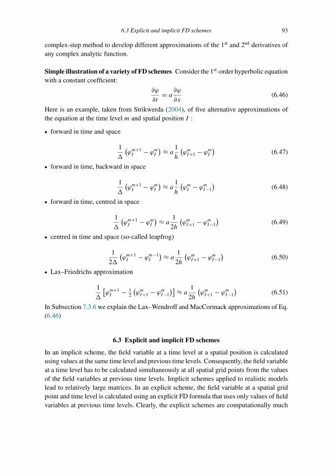
Trim: 247mm × 174mm Top: 14.762mm Gutter: 23.198mmCUUK2497-06 CUUK2497/Moczo ISBN: 978 1 107 02881 4 November 15, 2013 13:32
6.3 Explicit and implicit FD schemes 93
complex-step method to develop different approximations of the 1st and 2nd derivatives ofany complex analytic function.
Simple illustration of a variety of FD schemes Consider the 1st-order hyperbolic equationwith a constant coefficient:
∂ϕ
∂t= a ∂ϕ
∂x(6.46)
Here is an example, taken from Strikwerda (2004), of five alternative approximations ofthe equation at the time level m and spatial position I :
� forward in time and space
1
�
(ϕm+1I − ϕmI
) ≈ a 1
h
(ϕmI+1 − ϕmI
)(6.47)
� forward in time, backward in space
1
�
(ϕm+1I − ϕmI
) ≈ a 1
h
(ϕmI − ϕmI−1
)(6.48)
� forward in time, centred in space
1
�
(ϕm+1I − ϕmI
) ≈ a 1
2h
(ϕmI+1 − ϕmI−1
)(6.49)
� centred in time and space (so-called leapfrog)
1
2�
(ϕm+1I − ϕm−1
I
) ≈ a 1
2h
(ϕmI+1 − ϕmI−1
)(6.50)
� Lax–Friedrichs approximation
1
�
[ϕm+1I − 1
2
(ϕmI+1 − ϕmI−1
)] ≈ a 1
2h
(ϕmI+1 − ϕmI−1
)(6.51)
In Subsection 7.3.6 we explain the Lax–Wendroff and MacCormack approximations of Eq.(6.46)
6.3 Explicit and implicit FD schemes
In an implicit scheme, the field variable at a time level at a spatial position is calculatedusing values at the same time level and previous time levels. Consequently, the field variableat a time level has to be calculated simultaneously at all spatial grid points from the valuesof the field variables at previous time levels. Implicit schemes applied to realistic modelslead to relatively large matrices. In an explicit scheme, the field variable at a spatial gridpoint and time level is calculated using an explicit FD formula that uses only values of fieldvariables at previous time levels. Clearly, the explicit schemes are computationally much

Trim: 247mm × 174mm Top: 14.762mm Gutter: 23.198mmCUUK2497-06 CUUK2497/Moczo ISBN: 978 1 107 02881 4 November 15, 2013 13:32
94 Brief introduction to the finite-difference method
simpler. Therefore, explicit FD schemes have been used in most earthquake ground motionmodelling and exploration seismology studies.
An interesting example was presented by Geller and Takeuchi (1998). Their optimizationof the classical 2nd-order FD displacement scheme led to an implicit FD scheme (theynamed it the optimally accurate scheme) because they approximated the spatial derivativeas a weighted average of approximations at three time levels, and, similarly, the temporalderivative as a weighted average of approximations at three spatial positions. In order toavoid solving large systems of algebraic equations, Geller and Takeuchi applied a predictor-corrector scheme.
In compact schemes (e.g., Lele 1992) the spatial derivative at one spatial position iscalculated using both spatial derivatives and values at neighbouring grid positions. As aconsequence, the compact schemes are implicit.
For the implicit schemes see also, e.g., Emerman et al. (1982), Mufti (1985), Liu andSen (2009).
6.4 Basic properties of FD schemes
An FD scheme should be consistent with the original problem, stable and convergent. Herewe very briefly characterize these three properties. We recommend more mathematicallyoriented books for more detailed exposition and analysis: e.g., Isaacson and Keller (1966),Richtmyer and Morton (1967), Mitchell (1969), Marchuk (1982), Mitchell and Griffiths(1994), Morton and Mayers (1994), Thomas (1995), Shashkov (1996), Durran (1999),Cohen (2002), Forsythe and Wasow (2004), Strikwerda (2004), LeVeque (2007).
We use here the abbreviation FDEQ for FD equations or FD scheme, and EQ for apartial differential equation.
Consistency An FDEQ is consistent with the EQ if the difference between the FDEQ andthe EQ (the approximation or truncation error) vanishes as the sizes of the time step� andspatial grid spacing h go to zero independently, that is,
limh→0,�→0
|EQ − FDEQ| = 0 (6.52)
In most cases no relation between h and � is required. If, however, condition (6.52) istrue only when a certain relation is satisfied between h and �, the FDEQ is conditionallyconsistent.
Stability An FDEQ is stable if it produces a bounded solution when the exact solution isbounded, and is unstable if it produces an unbounded solution when the exact solution isbounded. If the solution of the FDEQ is bounded for all values of h and �, the FDEQ isunconditionally stable. If the solution of the FDEQ is bounded only for certain values of hand �, the FDEQ is conditionally stable. If the solution of the FDEQ is unbounded for allvalues of h and �, the FDEQ is unconditionally unstable.

Trim: 247mm × 174mm Top: 14.762mm Gutter: 23.198mmCUUK2497-06 CUUK2497/Moczo ISBN: 978 1 107 02881 4 November 15, 2013 13:32
6.4 Basic properties of FD schemes 95
The stability analysis can be performed only for a linear EQ. A nonlinear EQ must befirst linearized locally. The FDEQ of the linearized EQ can be analyzed for stability. Thereare several methods for analyzing stability. Probably the best known is the von Neumannmethod. The basic idea of the von Neumann method is to represent a discrete solution ata time level and spatial grid point by a finite Fourier series, and examine stability of theindividual Fourier components. In this sense the method investigates the local stability. Thediscrete solution is stable if and only if each Fourier component is stable.
The von Neumann method and also other methods of stability analysis are applicableto linear FDEQ with constant coefficients; in other words, for a homogeneous medium.Therefore, the stability condition found for the homogeneous medium has, in fact, anindicative meaning and should be checked in numerical computations for heterogeneousmedia.
Note that the explicit schemes can be only conditionally stable, whereas some implicitschemes can be unconditionally stable.
Convergence An FDEQ is convergent if the solution of the FDEQ approaches the exactsolution of the EQ as the sizes of the time step and spatial grid spacing go to zero.Denoting the solutions obtained by the EQ and FDEQ as ϕmI,K,L and �mI,K,L respectively,the convergence means
limh→0,�→0
∣∣�mI,K,L − ϕmI,K,L∣∣ = 0 (6.53)
It is important to note that the consistency is the property of the FDEQ because it relatesthe FDEQ to the EQ. On the other hand, stability and convergence are properties of thenumerical solution of the FDEQ.
Lax equivalence theorem In general, while it is easy to analyze the consistency, provingconvergence can be a very difficult mathematical problem. Therefore, it is very helpfulthat the convergence is related to the consistency and the stability: it follows from the Laxequivalence theorem that if the FDEQ is consistent and stable, it is also convergent.
Grid dispersion Because the FD solution is a discrete approximation of a true solution,the phase and group velocities in the grid in general differ from the true velocities in themedium. Grid dispersion is a very important grid phenomenon. It has a cumulative effecton wave propagation – the longer the travel distance, the larger the effect of the differencebetween the grid and true velocity. Therefore, grid dispersion has to be analyzed prior to thenumerical calculations. Given the desired travel path, one has to choose appropriate spatialsampling of the minimum wavelength to be propagated with a desired level of accuracy.
The grid-dispersion relation is a relation comprising frequency (real or grid), wavenum-ber (grid or real, respectively), grid spacing, time step and true physical speed(s) of themedium. Due to discretization, the dispersion relation in the grid differs from the dispersionrelation between frequency and wavenumber in the true physical continuum. The dispersion

Trim: 247mm × 174mm Top: 14.762mm Gutter: 23.198mmCUUK2497-06 CUUK2497/Moczo ISBN: 978 1 107 02881 4 November 15, 2013 13:32
96 Brief introduction to the finite-difference method
relation can be obtained from the stability analysis. Such analysis is feasible for many FDschemes assuming a homogeneous medium. It may be very complicated for heterogeneousmedia. Consequently, the effects of grid dispersion should be examined by careful numer-ical tests if the scheme is to be applied to heterogeneous media – which, in fact, is almostalways the case.
For a detailed analysis of stability, grid dispersion and accuracy of the FD schemes insolving the equation of motion in 2D and 3D problems in homogeneous media see, e.g.,articles by Marfurt (1984), Crase et al. (1992), Geller and Takeuchi (1995, 1998), Igel et al.(1995), Klimes (1996), Mizutani et al. (2000), Moczo et al. (2000), Takeuchi and Geller(2000), Zingg (2000), Liu and Sen (2011a,b), Geller et al. (2012).
6.5 Approximations based on a dispersion-relation-preserving criterion
Tam and Webb (1993) presented an interesting approach for finding FD approximations.They pointed out that the quality of FD schemes (in computational fluid dynamics) isgenerally ranked by the order of the Taylor series expansion truncation. For example,a 4th-order scheme should be better than a 2nd-order scheme. They claim that whereasfor time-independent problems such a criterion is quite sufficient, for time-dependentproblems, especially acoustics problems, a consistent, stable and convergent higher-orderscheme does not guarantee a good quality numerical wave solution. Their basic argumentis: the propagation characteristics of the waves governed by a system of partial differentialequations are encoded in the dispersion relation in the frequency and wavenumber space.Therefore, what is needed is an FD scheme that has the same or almost the same dispersionrelation as the original partial differential equations.
The dispersion relation may be obtained by applying the space and time Fourier trans-forms to the governing equations. If the dispersion relation is to be preserved then the FDapproximation should be constructed so that the Fourier transform is preserved. In otherwords, an FD approximation should have nearly the same Fourier transform in space ortime as the original partial derivative.
Hixon (1997) used the dispersion-relation-preserving (DRP) approach of Tam and Webb(1993) and developed one-sided (forward and backward) approximations of the first deriva-tive. Zhang and Chen (2006) and Zhang et al. (2012) applied a combination of the forwardand backward DRP approximations developed by Hixon (1997) in their FD modelling. Wewill address their scheme in Chapter 7.
Tam and Webb (1993) also showed that it is possible to combine the truncated Taylorseries FD approximation and the wavenumber space approximation.

Trim: 247mm × 174mm Top: 14.762mm Gutter: 23.198mmCUUK2497-07 CUUK2497/Moczo ISBN: 978 1 107 02881 4 November 15, 2013 13:36
7
1D problem
It is certainly very useful and instructive to introduce FD schemes in the case of the 1Dproblem. Many essential concepts and approaches can be explained without the unnecessarycomplexity of the 2D or 3D problems. Clearly, on the other hand, the 1D problem does notmake it possible to introduce and distinguish important aspects of different FD schemesthat emerge in 2D and 3D. One important example is the approximation of the 2nd mixedspatial derivatives in the displacement formulation. The consistency of the approximationsof the 2nd mixed and nonmixed spatial derivatives is closely related to the accuracy ofnumerical schemes with respect to the VP /VS ratio.
The explanations in this chapter are essential for understanding the following chapters.
7.1 Equation of motion and the stress–strain relation
Consider a Cartesian coordinate system with spatial coordinates (x, y, z) or, interchange-ably, (x1, x2, x3). (Indices 1, 2, 3 and letters x, y, z can be also used interchangeably assubscripts in order to denote displacement-vector and stress-tensor components). Considera perfectly elastic isotropic medium with density ρ (x) and Lame elastic coefficients μ (x)and λ (x) being continuous functions of the spatial coordinate x. Let �u (x, t) and σij (x, t)be the displacement vector and stress tensor, respectively. This defines a 1D problem alongthe x-axis. Table 7.1 shows wave-propagation configurations that can be described by thesame form of equations. P means the longitudinal wave. If the x- and y-axes are horizontal,then SH and SV denote shear waves polarized in the horizontal and vertical directions,respectively.
Denoting the appropriate displacement-vector and stress-tensor components by u andσ , respectively, and the appropriate elastic modulus by M , the strong-form equationsof motion and the stress–strain relation, i.e., Hooke’s law, can be written in one of thealternative formulations (omitting the body-force term):
Displacement–stress (DS) formulation
ρ∂2u
∂t2= ∂σ
∂x, σ = M∂u
∂x(7.1)
97
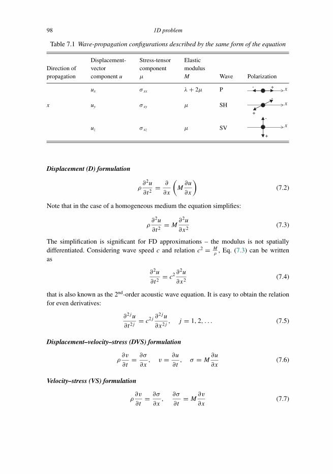
Trim: 247mm × 174mm Top: 14.762mm Gutter: 23.198mmCUUK2497-07 CUUK2497/Moczo ISBN: 978 1 107 02881 4 November 15, 2013 13:36
98 1D problem
Table 7.1 Wave-propagation configurations described by the same form of the equation
Direction ofpropagation
Displacement-vectorcomponent u
Stress-tensorcomponentμ
ElasticmodulusM Wave Polarization
ux σ xx λ + 2μ P x+-
x uy σ xy μ SH x
+
-
uz σ xz μ SV x
+
-
Displacement (D) formulation
ρ∂2u
∂t2= ∂
∂x
(M∂u
∂x
)(7.2)
Note that in the case of a homogeneous medium the equation simplifies:
ρ∂2u
∂t2= M∂
2u
∂x2(7.3)
The simplification is significant for FD approximations – the modulus is not spatiallydifferentiated. Considering wave speed c and relation c2 = M
ρ, Eq. (7.3) can be written
as
∂2u
∂t2= c2 ∂
2u
∂x2(7.4)
that is also known as the 2nd-order acoustic wave equation. It is easy to obtain the relationfor even derivatives:
∂2ju
∂t2j= c2j ∂
2ju
∂x2j, j = 1, 2, . . . (7.5)
Displacement–velocity–stress (DVS) formulation
ρ∂v
∂t= ∂σ
∂x, v = ∂u
∂t, σ = M∂u
∂x(7.6)
Velocity–stress (VS) formulation
ρ∂v
∂t= ∂σ
∂x,∂σ
∂t= M ∂v
∂x(7.7)
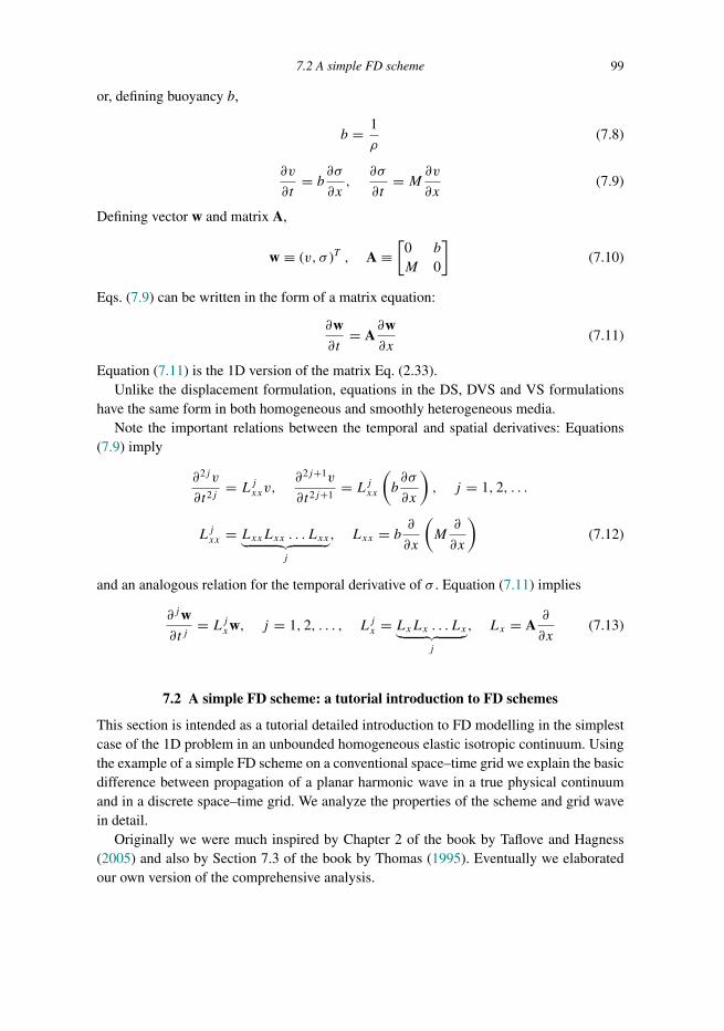
Trim: 247mm × 174mm Top: 14.762mm Gutter: 23.198mmCUUK2497-07 CUUK2497/Moczo ISBN: 978 1 107 02881 4 November 15, 2013 13:36
7.2 A simple FD scheme 99
or, defining buoyancy b,
b = 1
ρ(7.8)
∂v
∂t= b∂σ
∂x,∂σ
∂t= M ∂v
∂x(7.9)
Defining vector w and matrix A,
w ≡ (v, σ )T , A ≡[
0 b
M 0
](7.10)
Eqs. (7.9) can be written in the form of a matrix equation:
∂w∂t
= A∂w∂x
(7.11)
Equation (7.11) is the 1D version of the matrix Eq. (2.33).Unlike the displacement formulation, equations in the DS, DVS and VS formulations
have the same form in both homogeneous and smoothly heterogeneous media.Note the important relations between the temporal and spatial derivatives: Equations
(7.9) imply
∂2j v
∂t2j= Ljxxv,
∂2j+1v
∂t2j+1= Ljxx
(b∂σ
∂x
), j = 1, 2, . . .
Ljxx = LxxLxx . . . Lxx︸ ︷︷ ︸j
, Lxx = b ∂∂x
(M∂
∂x
)(7.12)
and an analogous relation for the temporal derivative of σ . Equation (7.11) implies
∂jw∂tj
= Ljxw, j = 1, 2, . . . , Ljx = LxLx . . . Lx︸ ︷︷ ︸j
, Lx = A∂
∂x(7.13)
7.2 A simple FD scheme: a tutorial introduction to FD schemes
This section is intended as a tutorial detailed introduction to FD modelling in the simplestcase of the 1D problem in an unbounded homogeneous elastic isotropic continuum. Usingthe example of a simple FD scheme on a conventional space–time grid we explain the basicdifference between propagation of a planar harmonic wave in a true physical continuumand in a discrete space–time grid. We analyze the properties of the scheme and grid wavein detail.
Originally we were much inspired by Chapter 2 of the book by Taflove and Hagness(2005) and also by Section 7.3 of the book by Thomas (1995). Eventually we elaboratedour own version of the comprehensive analysis.
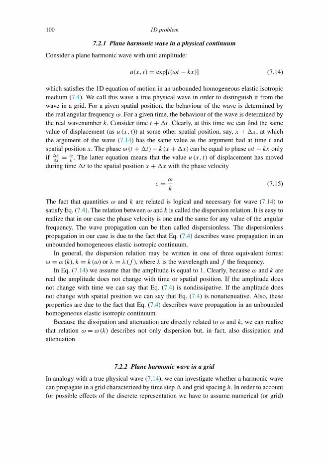
Trim: 247mm × 174mm Top: 14.762mm Gutter: 23.198mmCUUK2497-07 CUUK2497/Moczo ISBN: 978 1 107 02881 4 November 15, 2013 13:36
100 1D problem
7.2.1 Plane harmonic wave in a physical continuum
Consider a plane harmonic wave with unit amplitude:
u(x, t) = exp[i(ωt − kx)] (7.14)
which satisfies the 1D equation of motion in an unbounded homogeneous elastic isotropicmedium (7.4). We call this wave a true physical wave in order to distinguish it from thewave in a grid. For a given spatial position, the behaviour of the wave is determined bythe real angular frequency ω. For a given time, the behaviour of the wave is determined bythe real wavenumber k. Consider time t +�t . Clearly, at this time we can find the samevalue of displacement (as u (x, t)) at some other spatial position, say, x +�x, at whichthe argument of the wave (7.14) has the same value as the argument had at time t andspatial position x. The phase ω (t +�t) − k (x +�x) can be equal to phase ωt − kx onlyif �x�t
= ωk
. The latter equation means that the value u (x, t) of displacement has movedduring time �t to the spatial position x +�x with the phase velocity
c = ω
k(7.15)
The fact that quantities ω and k are related is logical and necessary for wave (7.14) tosatisfy Eq. (7.4). The relation between ω and k is called the dispersion relation. It is easy torealize that in our case the phase velocity is one and the same for any value of the angularfrequency. The wave propagation can be then called dispersionless. The dispersionlesspropagation in our case is due to the fact that Eq. (7.4) describes wave propagation in anunbounded homogeneous elastic isotropic continuum.
In general, the dispersion relation may be written in one of three equivalent forms:ω = ω (k), k = k (ω) or λ = λ (f ), where λ is the wavelength and f the frequency.
In Eq. (7.14) we assume that the amplitude is equal to 1. Clearly, because ω and k arereal the amplitude does not change with time or spatial position. If the amplitude doesnot change with time we can say that Eq. (7.4) is nondissipative. If the amplitude doesnot change with spatial position we can say that Eq. (7.4) is nonattenuative. Also, theseproperties are due to the fact that Eq. (7.4) describes wave propagation in an unboundedhomogeneous elastic isotropic continuum.
Because the dissipation and attenuation are directly related to ω and k, we can realizethat relation ω = ω (k) describes not only dispersion but, in fact, also dissipation andattenuation.
7.2.2 Plane harmonic wave in a grid
In analogy with a true physical wave (7.14), we can investigate whether a harmonic wavecan propagate in a grid characterized by time step� and grid spacing h. In order to accountfor possible effects of the discrete representation we have to assume numerical (or grid)

Trim: 247mm × 174mm Top: 14.762mm Gutter: 23.198mmCUUK2497-07 CUUK2497/Moczo ISBN: 978 1 107 02881 4 November 15, 2013 13:36
7.2 A simple FD scheme 101
quantities ω and k, which can differ from the true physical ω and k. The numerical (or grid)wave is
umI = exp[i(ωm�− kIh)] (7.16)
In general ω and k can be complex:
ω = ωreal + iωimag, k = kreal + ikimag (7.17)
Then,
umI = exp{i[(ωreal + iωimag
)m�− (
kreal + ikimag)Ih]}
= exp(−ωimagm�+ kimagIh
)exp
[i(ωrealm�− krealIh
)] (7.18)
It is clear that with nonzero imaginary parts of ω and/or k the amplitude of the gridwave is not equal to 1. ωimag and kimag determine dissipation in time and attenuation inspace, respectively. The real parts ωreal and kreal determine propagation in time and space,respectively. Consequently, the grid phase velocity is
v ≡ ωreal
kreal(7.19)
Obviously, with nonzero ωimag and/or kimag the phase velocity does not mean the velocityof propagation of a particular value of displacement, as was the case for a true physicalwave. Note also that even if the grid ω and k are real, they are not necessarily equal to thetrue physical ω and k.
7.2.3 The (2,2) 1D FD scheme on a conventional grid
Assume a conventional discrete space–time grid with time step � and grid spacing h.Use the centred 2nd-order FD approximation to replace both the temporal and spatial 2nd
derivatives in Eq. (7.4). Then the partial differential equation can be approximated by theFD equation:
1
�2
(um+1I − 2umI + um−1
I
) = c2 1
h2
(umI+1 − 2umI + umI−1
)(7.20)
from which we have an explicit FD scheme:
um+1I = 2umI − um−1
I +(c�
h
)2 (umI+1 − 2umI + umI−1
)(7.21)
Denote
EQ ≡ ∂2u
∂t2− c2 ∂
2u
∂x2
FDEQ ≡ 1
�2
(um+1I − 2umI + um−1
I
)− c2 1
h2
(umI+1 − 2umI + umI−1
) (7.22)

Trim: 247mm × 174mm Top: 14.762mm Gutter: 23.198mmCUUK2497-07 CUUK2497/Moczo ISBN: 978 1 107 02881 4 November 15, 2013 13:36
102 1D problem
Then the truncation error of the FD approximation of the partial differential equation is
TrunErr {FDEQ} = TaylorExpansion {FDEQ} − EQ
= 1
12
(∂4u
∂t4�2 − c2 ∂
4u
∂x4h2
)+O(�4) +O(h4)
(7.23)
Equation (7.23) means that the FD equation (7.20) is consistent with the differential equation(7.4) with 2nd-order accuracy both in time and space. Further, we will indicate the 2nd-orderaccuracy in time and space using abbreviation (2,2). Thus, in this case we can say thatscheme (7.21) is a (2,2) FD scheme.
Whereas Eq. (7.4) describes wave propagation in an unbounded homogeneous elasticisotropic continuum, Eq. (7.20) describes wave propagation in a discrete representation ofthe continuum. Whereas a true continuum is characterized by the wave speed c, its discreterepresentation is characterized by the true wave speed c, time step � and grid spacingh. Moreover, for given c, � and h, the wave propagation depends also on the schemeitself – Eq. (7.20) is just one of many possible approximations that are consistent withEq. (7.4).
We substitute displacement (7.16) for discrete displacement in Eq. (7.20). Denoting ther.h.s. of Eq. (7.16) by E, we obtain
umI = Eum+1I = E exp [i (ω�)] um−1
I = E exp [i (−ω�)]
umI+1 = E exp[i(−kh)] umI−1 = E exp[i(kh)]
(7.24)
and Eq. (7.20) transforms into
cos(ω�) − 1 = (c�
h)2[cos(kh) − 1] (7.25)
from which we obtain two equivalent numerical (or discrete) dispersion relations:
ω = 1
�arccos{1 + (c
�
h)2[cos(kh) − 1]} (7.26)
or
k = 1
harccos
{1 +
(h
c�
)2
[cos (ω�) − 1]
}(7.27)
The relations are sometimes called dispersion–dissipation relations. Denoting
S ≡ c�h
(7.28)
we have
ω = 1
�arccos{1 + S2[cos(kh) − 1]} (7.29)

Trim: 247mm × 174mm Top: 14.762mm Gutter: 23.198mmCUUK2497-07 CUUK2497/Moczo ISBN: 978 1 107 02881 4 November 15, 2013 13:36
7.2 A simple FD scheme 103
or
k = 1
harccos
{1 + 1
S2[cos (ω�) − 1]
}(7.30)
It is obvious that the dispersion relation obtained for a planar wave propagating in thegrid and governed by the FD Eq. (7.20) is fundamentally different from the dispersionrelation (7.15) of the true harmonic wave in a physical continuum. We have to analyze thegrid-dispersion relation in order to find the differences between the true and grid harmonicwaves.
The two alternative dispersion relations (7.29) and (7.30) naturally lead us to formulatetwo alternative partial problems, respectively:
(a) Assume a harmonic wave with k and ω propagating in a true physical continuumwithout dispersion. Assume a grid wave with k = k. What will be the grid angularfrequency ω?
(b) Assume a harmonic wave withω and k propagating in a true physical continuum withoutdispersion. Assume a grid wave with ω = ω. What will be the grid wavenumber k?
We will answer the two questions by investigating the behaviour of the grid wave with timeand spatial position.
Before we proceed, note that relation (7.25) could be written as
sin2 ω�
2= S2 sin2 kh
2(7.31)
7.2.4 Analysis of grid-dispersion relations
7.2.4.1 Behaviour of a grid wave with time: grid ω for a wave with physical k – Part 1
The behaviour of the grid wave with time is determined by the grid angular frequency ω.The grid wavenumber k can be considered a parameter – real and not different from thephysical k. The real k means that the amplitude does not change with spatial position.
Assuming complex ω and real k, the displacement at the spatial position I and time levelm can be written as
umI = exp{i[(ωreal + iωimag)m�− kIh]}= exp (−ωimagm�) exp[i(ωrealm�− kIh)]
(7.32)
The value of ωimag determines the behaviour of the amplitude with time:
ωimag > 0: the amplitude exponentially decreases with time at a given spatial position;the scheme is dissipative,
ωimag = 0: the amplitude remains constant with time at a given spatial position; thescheme is nondissipative,
ωimag < 0: the amplitude exponentially increases with time at a given spatial position;the scheme is unstable.
Trim: 247mm × 174mm Top: 14.762mm Gutter: 23.198mmCUUK2497-07 CUUK2497/Moczo ISBN: 978 1 107 02881 4 November 15, 2013 13:36
104 1D problem
Before we proceed, note that even if we considered k complex, the following analysisof the behaviour with time would not change: the imaginary part of k would just leadto a contribution to the amplitude at a given spatial position. The contributions would bedifferent at different spatial positions but would not change with time.
The argument of the cosine in the dispersion relation (7.29) can be expressed as
kh = kh = 2πh
λ(7.33)
It is reasonable to define the spatial sampling as
Nλ ≡ λ
h(7.34)
(Note that we define Nλ here – in the investigation of the behaviour of the grid wave withtime. This is an important difference compared to the definition by Taflove and Hagness,2005. We explain this in Subsection 7.2.5.) Then,
ω = 1
�arccos
{1 + S2
[cos
(2π
Nλ
)− 1
]}(7.35)
Denoting
ξ = 1 + S2
[cos
(2π
Nλ
)− 1
](7.36)
and using relation
arccos ξ = π
2− arcsin ξ (7.37)
we can write the dispersion relation (7.29) for ω as
ω = 1
�
(π2
− arcsin ξ)
(7.38)
7.2.4.2 Behaviour of a grid wave with spatial position: grid k for a wavewith physical ω – Part 1
The behaviour of the grid wave with spatial position is determined by the grid wavenumberk. The grid angular frequency ω can be considered a parameter – real and not different fromthe physical ω. The real ω means that the amplitude of the grid wave does not change withtime.
Assuming complex k and real ω, the displacement at spatial position I and time levelmcan be written as
umI = exp{i[ωm�− (kreal + ikimag)Ih]} = exp (kimagIh) exp[i(ωm�− krealIh)]
(7.39)
Trim: 247mm × 174mm Top: 14.762mm Gutter: 23.198mmCUUK2497-07 CUUK2497/Moczo ISBN: 978 1 107 02881 4 November 15, 2013 13:36
7.2 A simple FD scheme 105
The value of kimag determines the behaviour of the amplitude with spatial position:
kimag > 0: the amplitude exponentially increases with spatial position at a given time,kimag = 0 : the amplitude does not change with spatial position at a given time; the
scheme is nonattenuative,kimag < 0: the amplitude exponentially decreases with spatial position at a given time;
the scheme attenuates the wave in the grid.
Recall the dispersion relation for the grid wavenumber (7.30):
k = 1
harccos
{1 + 1
S2[cos (ω�) − 1]
}The argument of the cosine in the dispersion relation can be written as
ω� = ω� = 2π
T� (7.40)
It is reasonable to define the time sampling as
NT ≡ T
�(7.41)
Then,
k = 1
harccos
{1 + 1
S2
[cos
(2π
NT
)− 1
]}(7.42)
Denoting
ζ = 1 + 1
S2
[cos
(2π
NT
)− 1
](7.43)
and using relation (7.37) for ζ the dispersion relation becomes
k = 1
h
(π2
− arcsin ζ)
(7.44)
7.2.4.3 Behaviour of a grid wave with time and spatial position: a joint part
Both dispersion relations (7.38) and (7.44) have the form
ϕ = 1
δ
(π2
− arcsinχ)
(7.45)
where {ϕ, δ, χ}, stand for {ω,�, ξ } or{k, h, ζ
}, respectively. Considering the definition of
the function arcsin it is reasonable to investigate the case when χ is from interval 〈−1, 1〉,and the case when χ is outside interval 〈−1, 1〉.The case: −1 ≤ χ ≤ 1
It follows from −π2 ≤ arcsinχ ≤ π
2 and Eq. (7.45) that
ϕ = 1
δ
(π2
− arcsinχ), 0 ≤ ϕreal ≤ π
δ, ϕimag = 0 (7.46)

Trim: 247mm × 174mm Top: 14.762mm Gutter: 23.198mmCUUK2497-07 CUUK2497/Moczo ISBN: 978 1 107 02881 4 November 15, 2013 13:36
106 1D problem
In order to consider χ outside interval 〈−1, 1〉, use the relation (e.g., Korn and Korn 2000,p. 817)
arcsinχ = −i ln(iχ +
√1 − χ2
)(7.47)
The case: χ > 1Rewrite relation (7.47) as follows:
arcsinχ = −i ln(iχ +
√1 − χ2
)= − i ln
(iχ + i
√χ2 − 1
) = −i ln[exp
(i π2)(χ +
√χ2 − 1
)]= − i{ln [exp
(i π2)]+ ln
(χ +
√χ2 − 1
)}= − i{i π2 + ln
(χ +
√χ2 − 1
)} = π2 − i ln
(χ +
√χ2 − 1
)Then,
ϕ = i 1δ
ln(χ +
√χ2 − 1
), ϕreal = 0, ϕimag = 1
δln(χ +
√χ2 − 1
)(7.48)
The case: χ < −1Rewrite relation (7.47) as follows:
arcsinχ = −i ln[i(χ +
√χ2 − 1
)] = −i ln[−i(−χ −
√χ2 − 1
)]= − i ln
[exp
(−i π
2
) (−χ −√χ2 − 1
)]= − i
{ln[exp
(−i π
2
)]+ ln
(−χ −√χ2 − 1
)}= − i
{−i π
2+ ln
(−χ −√χ2 − 1
)} = −π2
− i ln(−χ −
√χ2 − 1
)Then,
ϕ = 1
δ
[π + i ln
(−χ −√χ2 − 1
)](7.49)
ϕreal = π
δ, ϕimag = 1
δln(−χ −
√χ2 − 1
)< 0
The latter inequality is due to the fact that the argument of the logarithm is positive andsmaller than 1.
Having obtained relations (7.46), (7.48) and (7.49) for −1 ≤ χ ≤ 1, χ > 1 and χ < −1,respectively, we can continue with the analysis of the scheme.
7.2.4.4 Behaviour of a grid wave with time: grid ω for a wave with physical k – Part 2
Because 2πNλ
is real, −1 ≤ cos(
2πNλ
) ≤ 1. It follows from Eq. (7.36) that
1 − 2S2 ≤ ξ ≤ 1 (7.50)
Recall that S > 0, see Eq. (7.28). We can recognize two cases.
Trim: 247mm × 174mm Top: 14.762mm Gutter: 23.198mmCUUK2497-07 CUUK2497/Moczo ISBN: 978 1 107 02881 4 November 15, 2013 13:36
7.2 A simple FD scheme 107
The case: −1 ≤ ξ ≤ 1Investigate when −1 ≤ ξ ≤ 1. It is clear from condition (7.50) that always ξ ≤ 1.
Substituting definition (7.36) for ξ in the condition −1 ≤ ξ we can obtain
S2 ≤ 2
1 − cos
(2π
Nλ
) (7.51)
Thus, if S satisfies condition (7.51), −1 ≤ ξ ≤ 1, and, according to (7.46),
ω = 1
�
(π2
− arcsin ξ), 0 ≤ ωreal ≤ π
�, ωimag = 0 (7.52)
Recalling Eq. (7.29),
ω = ωreal = 1
�arccos
{1 + S2
[cos
(2π
Nλ
)− 1
]}(7.53)
Equivalently,
ω = ωreal
= 1
�arccos
{1 + S2 [cos (kh) − 1]
}= 1
�arccos
{1 + S2
[cos
(ω�
S
)− 1
]} (7.54)
Referring to Eq. (7.32) we obtain the first partial conclusion on the behaviour of the gridwave with time if S satisfies condition (7.51):
(a) Whereas a harmonic wave with k and ω can propagate in a true physical continuumwithout dispersion, a grid wave with k = k can propagate with grid dispersion and itsangular frequency ω is given by relation (7.53) or (7.54).
(b) At any spatial grid position the amplitude of a harmonic wave does not change withtime. The numerical scheme is nondissipative.
The case: ξ < −1Investigate now when ξ < −1. Substituting definition (7.36) for ξ in the latter conditionwe can obtain
S2 >2
1 − cos
(2π
Nλ
) (7.55)
Thus, if S satisfies condition (7.55), ξ < −1, and, according to (7.49),
ω = 1
�
[π + i ln
(−ξ −√ξ 2 − 1
)]ωreal = π
�, ωimag = 1
�ln(−ξ −
√ξ 2 − 1
)< 0
(7.56)
Referring again to Eq. (7.32) we obtain the second partial conclusion on the behaviour ofthe grid wave with time if S satisfies condition (7.55):
(c) Whereas a harmonic wave with k and ω can propagate in a true physical contin-uum without dispersion, a grid wave with k = k can propagate with the grid angularfrequency ωreal = π
�.

Trim: 247mm × 174mm Top: 14.762mm Gutter: 23.198mmCUUK2497-07 CUUK2497/Moczo ISBN: 978 1 107 02881 4 November 15, 2013 13:36
108 1D problem
(d) At any spatial grid position the amplitude exponentially increases with time. Thescheme is unstable.
We can quantify the exponential increase of the amplitude. Because, see (7.32) and (7.56),
umI = exp(−ωimagm�
)exp
[i(ωrealm�− kIh)]
= exp[−m ln
(−ξ −√ξ 2 − 1
)]exp
[i(mπ − kIh)]
= exp[ln(−ξ −
√ξ 2 − 1
)−m]exp
[i(mπ − kIh)]
= 1(−ξ −√ξ 2 − 1
)m exp[i(mπ − kIh)]
the amplitude amplification factor per time step is
q =∣∣um+1I
∣∣∣∣umI ∣∣ = 1
−ξ −√ξ 2 − 1
= −ξ +√ξ 2 − 1 > 1 (7.57)
The smaller ξ is, the larger is q. The amplification factor q gains its maximum value forthe minimum value of ξ , that is for ξ = 1 − 2S2 (see Eq. (7.50)):
qmax = −(1 − 2S2) +√
(1 − 2S2)2 − 1 = (S +√S2 − 1)2 (7.58)
It follows from Eq. (7.36) that ξ gains its minimum value for 2πNλ
= π , that is, for Nλ = 2.Thus, the exponential increase of the amplitude is largest at wavelength
λU = 2h (7.59)
This exponential growth originates the numerical instability. The frequency of the unstablegrid wave is
fU = ωreal
2π= 1
2�(7.60)
being determined only by the time step �.
Stability We have identified two regimes of the scheme behaviour with time. The nondissi-pative or stable regime is determined by condition (7.51), the unstable regime is determinedby condition (7.55). The value of S, discriminating the two regimes, depends on Nλ. Thisis illustrated in Fig. 7.1.
In practice, however, we usually do not simulate one harmonic wave, that is, a wavewith one wavelength. We have a range of wavelengths. Therefore, for a given value of gridspacing h we have a range of Nλ values – the shorter the wavelength, the smaller is Nλ. Ifwe admit any positive value of Nλ, conditions (7.51) and (7.55) transform to
S ≤ 1 (7.61)

Trim: 247mm × 174mm Top: 14.762mm Gutter: 23.198mmCUUK2497-07 CUUK2497/Moczo ISBN: 978 1 107 02881 4 November 15, 2013 13:36
7.2 A simple FD scheme 109
2 3 4 5 6 7 8 9 10 11 120.0
0.5
1.0
1.5
2.0
2.5
3.0
3.5
4.0
unstable
S
Nλ
stable
Nλ
Figure 7.1 Value of factor S, discriminating the nondissipative (stable) and unstable regimes ofthe grid wave with physical wavelength, as a function of the spatial sampling Nλ of the physicalwavelength of one harmonic wave.
and
S > 1 (7.62)
respectively.For the analyzed scheme, 1 is the maximum value of S for which the analyzed FD
scheme is stable. It is reasonable to anticipate that for some other FD scheme the limitingvalue may be different from 1. Therefore, we denote the limiting value in general as SM .Consequently, a general form of the stability condition for 1D schemes can be written as
S ≤ SM (7.63)
From
S = c�h
≤ SM (7.64)
we have
� ≤ h
cSM (7.65)
Define the stability ratio p as
p ≡ c�
hSM(7.66)
Then,
0 < p ≤ 1 (7.67)
� = phcSM (7.68)
Trim: 247mm × 174mm Top: 14.762mm Gutter: 23.198mmCUUK2497-07 CUUK2497/Moczo ISBN: 978 1 107 02881 4 November 15, 2013 13:36
110 1D problem
Clearly, hcSM is the maximum time step for which the scheme is stable and p quantifies
the fraction of the maximum time step. Condition (7.61) for the analyzed scheme can bewritten as
S = pSM ; 0 < p ≤ 1, SM = 1 (7.69)
Thus, the main conclusion of the performed analysis of the scheme behaviour with time isthat it is necessary to choose
� = phcSM ; 0 < p ≤ 1, SM = 1 (7.70)
in order to prevent instability of the numerical solution. Factor S can be called the stabil-ity factor and relation (7.61), (7.69) or (7.70) the stability condition for the investigatednumerical scheme. Factor S is also known as the Courant number. Let us note that the namereflects the fundamental article by Courant, Friedrichs and Lewy (1928 in German, 1967 inEnglish translation) – the first article on the stability and convergence of the FD schemessolving partial differential equations. For more details see, e.g., LeVeque (2007).
Considering Eq. (7.69), relations (7.53) and (7.54) can be written as
ω = ωreal = 1
�arccos
{1 + p2
[cos
(2π
Nλ
)− 1
]}= 1
�arccos
{1 + p2 [cos (kh) − 1]
}= 1
�arccos
{1 + p2
[cos
(ω�
p
)− 1
]} (7.71)
7.2.4.5 Behaviour of a grid wave with spatial position: grid k for a wavewith physical ω – Part 2
Clearly we can apply the results of the joint part of the analysis also in the investigation ofthe behaviour of the grid wave with spatial position. In the investigation, however, we haveto account for the fact that we have found the stability condition (7.69) for S.
Because 2πNT
is real, −1 ≤ cos(
2πNT
) ≤ 1. It follows from Eq. (7.43) that
1 − 2
S2≤ ζ ≤ 1 (7.72)
and, using (7.69),
1 − 2
p2≤ ζ ≤ 1 (7.73)
We can recognize two cases.

Trim: 247mm × 174mm Top: 14.762mm Gutter: 23.198mmCUUK2497-07 CUUK2497/Moczo ISBN: 978 1 107 02881 4 November 15, 2013 13:36
7.2 A simple FD scheme 111
The case: −1 ≤ ζ ≤ 1Investigate when −1 ≤ ζ ≤ 1. It is clear from condition (7.72) that always ζ ≤ 1.
Substituting definition (7.43) for ζ in the condition −1 ≤ ζ and using (7.69) we can obtain
NT ≥ 2π
arccos(1 − 2p2)(7.74)
Relation (7.74) can be transformed into the frequency domain:
T = �NT ≥ 2π�
arccos(1 − 2p2)
f = 1
T≤ arccos(1 − 2p2)
π
1
2�
(7.75)
Define frequency fATT
fATT ≡ arccos(1 − 2p2)
πfN (7.76)
where fN is the Nyquist frequency
fN ≡ 1
2�(7.77)
The frequency-domain equivalent of condition (7.74) can be then written as
f ≤ fATT (7.78)
Thus, ifNT satisfies condition (7.74) or, equivalently, f satisfies condition (7.78), accordingto (7.46)
k = 1
h
(π2
− arcsin ζ), 0 < kreal ≤ π
2, kimag = 0 (7.79)
Recalling Eq. (7.42):
k = 1
harccos
{1 + 1
p2
[cos
(2π
NT
)− 1
]}(7.80)
Equivalently,
k = 1
harccos
{1 + 1
p2[cos (ω�) − 1]
}= 1
harccos
{1 + 1
p2[cos (pkh) − 1]
} (7.81)
Referring to Eq. (7.39) we obtain the first partial conclusion on the behaviour of a grid wavewith spatial position if NT satisfies condition (7.74) or, equivalently, f satisfies condition(7.78):
(a) Whereas a harmonic wave with ω and k can propagate in a true physical contin-uum without dispersion, a grid wave with ω = ω ≤ 2πfATT can propagate with grid
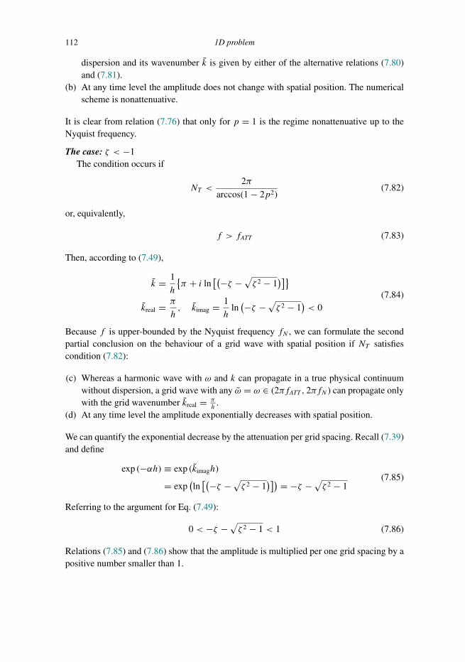
Trim: 247mm × 174mm Top: 14.762mm Gutter: 23.198mmCUUK2497-07 CUUK2497/Moczo ISBN: 978 1 107 02881 4 November 15, 2013 13:36
112 1D problem
dispersion and its wavenumber k is given by either of the alternative relations (7.80)and (7.81).
(b) At any time level the amplitude does not change with spatial position. The numericalscheme is nonattenuative.
It is clear from relation (7.76) that only for p = 1 is the regime nonattenuative up to theNyquist frequency.
The case: ζ < −1The condition occurs if
NT <2π
arccos(1 − 2p2)(7.82)
or, equivalently,
f > fATT (7.83)
Then, according to (7.49),
k = 1
h
{π + i ln
[(−ζ −√ζ 2 − 1
)]}kreal = π
h, kimag = 1
hln(−ζ −
√ζ 2 − 1
)< 0
(7.84)
Because f is upper-bounded by the Nyquist frequency fN , we can formulate the secondpartial conclusion on the behaviour of a grid wave with spatial position if NT satisfiescondition (7.82):
(c) Whereas a harmonic wave with ω and k can propagate in a true physical continuumwithout dispersion, a grid wave with any ω = ω ∈ (2πfATT , 2πfN ) can propagate onlywith the grid wavenumber kreal = π
h.
(d) At any time level the amplitude exponentially decreases with spatial position.
We can quantify the exponential decrease by the attenuation per grid spacing. Recall (7.39)and define
exp (−αh) ≡ exp (kimagh)
= exp(ln[(−ζ −
√ζ 2 − 1
)]) = −ζ −√ζ 2 − 1
(7.85)
Referring to the argument for Eq. (7.49):
0 < −ζ −√ζ 2 − 1 < 1 (7.86)
Relations (7.85) and (7.86) show that the amplitude is multiplied per one grid spacing by apositive number smaller than 1.

Trim: 247mm × 174mm Top: 14.762mm Gutter: 23.198mmCUUK2497-07 CUUK2497/Moczo ISBN: 978 1 107 02881 4 November 15, 2013 13:36
7.2 A simple FD scheme 113
0.0 0.2 0.4 0.6 0.8 1.00.0
0.1
0.2
0.3
0.4
0.5
attenuative
non-attenuativef AT
T, n
orm
aliz
ed
S
Figure 7.2 Value of the normalized frequency fATT,normalized, discriminating the nonattenuative andattenuative regimes of the grid wave with physical frequency, as a function of the stability ratio p forone harmonic wave.
Grid attenuation We have identified two regimes of the scheme behaviour with spatialposition. The nonattenuative regime is determined by condition (7.74) or (7.78), the attenu-ative regime is determined by condition (7.82) or (7.83). The value of fATT , discriminatingthe two regimes, depends on S.
Let us illustrate the relation between fATT and S numerically. Consider normalizedfrequency
fnormalized ≡ f� (7.87)
Correspondingly we define
fATT,normalized ≡ arccos (1 − 2p2)
2π(7.88)
Note that the normalized Nyquist frequency is
fN,normalized = 0.5 (7.89)
Figure 7.2 shows fATT,normalized as a function of the stability ratio S.We can also numerically illustrate the attenuation. Because
fnormalized = f� = 1
NT(7.90)
ζ defined by Eq. (7.43) and appearing in relation (7.85) can be written as
ζ = 1 + 1
p2[cos (2πfnormalized) − 1] (7.91)
Considering 2 ≤ NT <∞, we have 0 < fnormalized ≤ 12 .
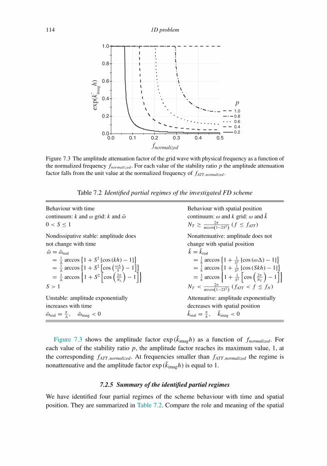
Trim: 247mm × 174mm Top: 14.762mm Gutter: 23.198mmCUUK2497-07 CUUK2497/Moczo ISBN: 978 1 107 02881 4 November 15, 2013 13:36
114 1D problem
0.0 0.1 0.2 0.3 0.4 0.50.0
0.2
0.4
0.6
0.8
1.0
pex
p(k~ im
agh)
fnormalized
1.0 0.8 0.6 0.4 0.2
Figure 7.3 The amplitude attenuation factor of the grid wave with physical frequency as a function ofthe normalized frequency fnormalized . For each value of the stability ratio p the amplitude attenuationfactor falls from the unit value at the normalized frequency of fATT,normalized.
Table 7.2 Identified partial regimes of the investigated FD scheme
Behaviour with time Behaviour with spatial positioncontinuum: k and ω grid: k and ω continuum: ω and k grid: ω and k0 < S ≤ 1 NT ≥ 2π
arccos(1−2S2) (f ≤ fATT )
Nondissipative stable: amplitude doesnot change with time
Nonattenuative: amplitude does notchange with spatial position
ω = ωreal
= 1�
arccos{1 + S2 [cos (kh) − 1]
}= 1
�arccos
{1 + S2
[cos
(ω�S
)− 1]}
= 1�
arccos{
1 + S2[cos
(2πNλ
)− 1
]}k = kreal
= 1h
arccos{1 + 1
S2 [cos (ω�) − 1]}
= 1h
arccos{1 + 1
S2 [cos (Skh) − 1]}
= 1h
arccos{
1 + 1S2
[cos
(2πNT
)− 1
]}S > 1 NT <
2πarccos(1−2S2) (fATT < f ≤ fN )
Unstable: amplitude exponentiallyincreases with time
Attenuative: amplitude exponentiallydecreases with spatial position
ωreal = π�, ωimag < 0 kreal = π
h, kimag < 0
Figure 7.3 shows the amplitude factor exp (kimagh) as a function of fnormalized. Foreach value of the stability ratio p, the amplitude factor reaches its maximum value, 1, atthe corresponding fATT,normalized. At frequencies smaller than fATT,normalized the regime isnonattenuative and the amplitude factor exp (kimagh) is equal to 1.
7.2.5 Summary of the identified partial regimes
We have identified four partial regimes of the scheme behaviour with time and spatialposition. They are summarized in Table 7.2. Compare the role and meaning of the spatial
Trim: 247mm × 174mm Top: 14.762mm Gutter: 23.198mmCUUK2497-07 CUUK2497/Moczo ISBN: 978 1 107 02881 4 November 15, 2013 13:36
7.2 A simple FD scheme 115
sampling Nλ and time sampling NT . Nλ quantifies sampling of the physical wavelength,which is also the grid wavelength. NT quantifies sampling of the physical period whichis also the grid period. Note that Nλ should not be used in the analysis of the behaviourwith spatial position because in that case it would quantify a wavelength that does notpropagate in the grid. Similarly, NT should not be used in the analysis of the behaviourwith time because in that case it would quantify a period that does not propagate in thegrid.
Obviously, for numerical simulation of wave propagation we need a conjunction ofthe nondissipative and nonattenuative regimes. If we choose S ≤ 1, the simulation will bestable. It will be nonattenuative up to frequency fATT .
We have found that grid wave propagation is not dispersionless in these regimes. Weshould therefore quantify grid dispersion in terms of grid phase velocity.
7.2.6 Grid phase and group velocities
7.2.6.1 Grid phase velocity
The grid phase velocity is given by Eq. (7.19):
v = ωreal
kreal
As we have found, we have two possibilities:
First possibility: Assume k = k and use the dispersion relation for ω.Second possibility: Assume ω = ω and use the dispersion relation for k.
The first possibility will lead to the grid phase velocity of the wave with a true physicalwavelength. The second one will lead to the grid phase velocity of the wave with a truephysical frequency.
Grid phase velocity of the wave with a true physical wavelengthRecalling relations (7.71) and (7.70) we obtain the following alternative relations for
stable wave propagation:
v = ωreal
k= 1
pkharccos
{1 + p2 [cos (kh) − 1]
}c
= 1
ω�arccos
{1 + p2
[cos
(ω�
p
)− 1
]}c
= Nλ
2πparccos
{1 + p2
[cos
(2π
Nλ
)− 1
]}c
(7.92)
The grid phase velocity given by any one of the relations (7.92) is the velocity of the gridwave that has the same wavelength λ as the true physical wave. The fourth of the relations

Trim: 247mm × 174mm Top: 14.762mm Gutter: 23.198mmCUUK2497-07 CUUK2497/Moczo ISBN: 978 1 107 02881 4 November 15, 2013 13:36
116 1D problem
2 4 6 8 10 12 14 16 18 200.65
0.70
0.75
0.80
0.85
0.90
0.95
1.00
pv~ /c
Nλ
1.0 0.8 0.6 0.4 0.2
2 4 6 8 10 12 14 16 18 200.65
0.70
0.75
0.80
0.85
0.90
0.95
1.00
pv~ G /c
Nλ
1.0 0.8 0.6 0.4 0.2
(a)
(b)
Nλ
Nλ
Figure 7.4 The normalized grid phase velocity (a) and normalized grid group velocity (b) of the gridwave with physical wavelength λ, as a function of the spatial samplingNλ of the physical wavelength.
(7.92) is useful for practical simulations because, for a given value of the stability ratio p,it directly relates grid phase velocity to spatial sampling Nλ. The normalized grid phasevelocities for five values of p are shown in Fig. 7.4a.
It is also interesting to look at the phase velocity of an unstable wave. Recalling relations(7.56) and (7.59), the phase velocity is
vU = ωreal
k= π
�
λU
2π= π
�
2h
2π= h
�= c
S(7.93)
The phase velocity of an unstable wave is surprisingly simply related to the stability factorS. Note that vU = h
�is the maximum possible grid phase velocity. A grid wave cannot
propagate a larger distance than h in one time step �.

Trim: 247mm × 174mm Top: 14.762mm Gutter: 23.198mmCUUK2497-07 CUUK2497/Moczo ISBN: 978 1 107 02881 4 November 15, 2013 13:36
7.2 A simple FD scheme 117
Grid phase velocity of the wave with a true physical frequencyWe obtain the following alternative relations for the nonattenuative regime:
v = ω
kreal= ω�
p arccos
{1 + 1
p2[cos (ω�) − 1]
}c= kh
arccos
{1 + 1
p2[cos (pkh) − 1]
}c= 2π
pNT arccos
{1 + 1
p2
[cos
(2π
NT
)− 1
]}c(7.94)
The grid phase velocity given by any one of the relations (7.94) is the velocity of the gridwave that has the same frequency as the true physical wave.
What is the phase velocity in the nondissipative (stable) but attenuative regime? Using(7.84) we obtain
v = ω
kreal= h
π
2π
T= 2
SNTc = 2
pNTc (7.95)
The grid phase velocity can be numerically illustrated. In order to compare the phasevelocity with attenuation, we rewrite the relations for the phase velocities (7.94) and (7.95)as functions of fnormalized:
for f ≤ fATT
v = 2πfnormalized
p arccos{
1 + 1p2 [cos (2πfnormalized) − 1]
}c (7.96)
for fATT < f ≤ fN
v = 2fnormalized
pc (7.97)
The upper panel of Fig. 7.5 shows the normalized grid phase velocity, the bottom panelshows the amplitude attenuation factor. Both panels clearly visualize the sudden change ofthe displayed quantities at fATT .
7.2.6.2 Grid group velocity
The existence of grid dispersion of the phase velocity implies the existence of the gridgroup velocity:
vG ≡ ∂ω
∂k(7.98)

Trim: 247mm × 174mm Top: 14.762mm Gutter: 23.198mmCUUK2497-07 CUUK2497/Moczo ISBN: 978 1 107 02881 4 November 15, 2013 13:36
118 1D problem
0.65
0.70
0.75
0.80
0.85
0.90
0.95
1.00
pv
/c~
1.0 0.8 0.6 0.4 0.2
0.0 0.1 0.2 0.3 0.4 0.50.0
0.2
0.4
0.6
0.8
1.0
p
exp(
k~ imag
h)
fnormalized
1.0 0.8 0.6 0.4 0.2
Figure 7.5 The normalized grid phase velocity (top panel) and the amplitude attenuation factor(bottom panel) of the grid wave with physical frequency ω as a function of the normalized frequencyfnormalized. For each value of the stability ratio p the normalized grid phase velocity has a sharpminimum at the normalized frequency of fATT,normalized. For each value of p the amplitude attenuationfactor falls from the unit value at fATT,normalized.
Recalling relations (7.53), (7.54), (7.69) and (7.70)
vG = ∂ω
∂k= p sin (kh)√
1 − {1 + p2 [cos (kh) − 1]
}2c
= psin
(2π
Nλ
)√
1 −{
1 + p2
[cos
(2π
Nλ
)− 1
]}2c
(7.99)
The normalized grid group velocities for five values of p are shown in Fig. 7.4b.

Trim: 247mm × 174mm Top: 14.762mm Gutter: 23.198mmCUUK2497-07 CUUK2497/Moczo ISBN: 978 1 107 02881 4 November 15, 2013 13:36
7.2 A simple FD scheme 119
7.2.7 Local error
Recall scheme (7.20):
um+1I = 2umI − um−1
I +(c�
h
)2 (umI+1 − 2umI + umI−1
)(7.100)
which can be written symbolically as
u (I, t +�) = numerical scheme {u (t −�) , u (t)} (7.101)
Define a numerical solution in one time step as
uN (I, t +�) ≡ numerical scheme{uE (t −�) , uE (t)
}(7.102)
where the upper index N indicates the numerical solution, and the upper index E indicatesan exact value. Because we consider
u (x, t) = exp [i (ωt − kx)] (7.103)
the exact displacement is complex. We can define a local error for real parts of the numericaland exact displacements as follows: a relative local error in amplitude is
εRelampl ≡
(�ref
�
)2 ∣∣∣∣AN − AE
AE
∣∣∣∣ =(�ref
�
)2 ∣∣∣∣AN
AE− 1
∣∣∣∣ (7.104)
where AN is the modulus of the real part of the numerical displacement in one time stepand AE is the modulus of the real part of the exact displacement – both evaluated at timet +�. If the local error is to be a general concept it has to be reasonably defined alsofor possible comparisons with other schemes. Because different numerical schemes usedifferent time steps, we have to normalize the error for a unit time. Because the timederivative is approximated with the 2nd-order accuracy, we have to normalize the error withthe square of �. The division gives the error a physical unit (s−2) and larger value. Thesecan be compensated, for example, by multiplication by the square of some time-step value�ref taken as a reference.
Without loss of generality, consider for simplicity
xI = 0, tm = 0 (7.105)
Then the errors are evaluated at
xI = 0, tm+1 = � (7.106)
The exact real displacement at this space–time grid position is
Re{uE (0,�)
} = cosω� (7.107)
and
AE = ∣∣Re{uE (0,�)
}∣∣ = |cosω�| (7.108)

Trim: 247mm × 174mm Top: 14.762mm Gutter: 23.198mmCUUK2497-07 CUUK2497/Moczo ISBN: 978 1 107 02881 4 November 15, 2013 13:36
120 1D problem
The exact complex displacements entering the r.h.s. of scheme (7.100) are
umI = 1 um−1I = exp (−iω�)
umI+1 = exp (−ikh) umI−1 = exp (+ikh)(7.109)
The numerical complex displacement at xI = 0 and tm+1 = � is
uN (0,�) = 2 − exp (−iω�) + S2[exp (−ikh) − 2 + exp (+ikh)
]= 2 − cosω�+ i sinω�+ 2S2 [cos kh− 1]
(7.110)
The real part of the numerical displacement is
Re{uN (0,�)
} = 2 − cosω�+ 2S2 [cos kh− 1] (7.111)
AN = ∣∣Re{uN (0,�)
}∣∣ = ∣∣2 − cosω�+ 2S2 [cos kh− 1]∣∣ (7.112)
Then,
εRelampl =
(�ref
�
)2∣∣∣∣∣∣∣2 − cosω�+ 2S2 [cos kh− 1]
∣∣|cosω�| − 1
∣∣∣∣∣ (7.113)
In the previous analyses we assumed either true physical k and grid ω or true physical ωand grid k. Here the values entering the scheme at time levels m− 1 and m are exact. Thismeans that both k and ω are assumed exact at both time levels:
kh = 2πh
λ= 2π
Nλ(7.114)
ω� = 2π
T� = 2π
λc ph
cSM︸ ︷︷ ︸�
= 2π
NλpSM (7.115)
Because SM = 1,
εRelampl =
(�ref
�
)2
∣∣∣∣∣∣∣∣
∣∣∣∣2 − cos
(2π
Nλp
)+ 2p2
[cos
(2π
Nλ
)− 1
]∣∣∣∣∣∣∣∣cos
(2π
Nλp
)∣∣∣∣− 1
∣∣∣∣∣∣∣∣ (7.116)
Note that (7.115) implies (�ref
�
)2
=(Nλ
Nλ,ref
)2
(7.117)
The local errors in amplitude for five values of p are shown in Fig. 7.6. Note that the erroris zero for p = 1.
Note on the local error and grid dispersion It is clear that the local error in amplitudequantifies how the exact amplitude changes in one time step due to inaccuracy of thenumerical scheme. In the analysis of grid dispersion we assume a constant amplitude of

Trim: 247mm × 174mm Top: 14.762mm Gutter: 23.198mmCUUK2497-07 CUUK2497/Moczo ISBN: 978 1 107 02881 4 November 15, 2013 13:36
7.2 A simple FD scheme 121
2 3 4 5 6 7 8 910 20
1E-5
1E-4
1E-3
0.01
0.1
εRel
ampl
Nλ
p 1.0 0.8 0.6 0.4 0.2
Nλ
Figure 7.6 The local error in amplitude as a function of the spatial sampling Nλ of the physicalwavelength. �ref is chosen as the time step for Nλ = 20. Note that the error is zero for p = 1 – thecorresponding line is missing.
the grid wave (wave propagating in the stable nonattenuative regime). In one analysiswe assume a grid wave with grid wavenumber k equal to the true wavenumber k andinvestigate how the grid frequency ω will be different from the true physical frequency ω.In the other analysis we assume a grid wave with frequency ω equal to the true frequencyω and investigate how the grid wavenumber k will be different from the true physicalwavenumber k. In both cases, the price for propagating the harmonic plane wave withconstant amplitude in a discrete grid is a grid velocity that differs from the true velocity,and the difference depends on the size of the grid spacing and time step.
7.2.8 Sufficiently accurate numerical simulation
Consider an unbounded homogeneous medium characterized by the true wave speed c. Con-sider that a wavefield is generated in the frequency range [fMIN, fMAX]. The correspondingrange of the wavelengths is [λMIN, λMAX] = [
cfMAX, cfMIN
].
We want to numerically simulate the wavefield using the analyzed FD scheme (7.20)sufficiently accurately for the range of wavelengths [λMIN, λMAX].
In order to prepare the numerical calculation we need to recall the stability condition,Eq. (7.70),
� = phcSM ; 0 < p ≤ 1, SM = 1 (7.118)
the grid dispersion of the phase velocity, Eq. (7.92) and Fig. 7.4,
v = Nλ
2πparccos
{1 + p2
[cos
(2π
Nλ
)− 1
]}c (7.119)

Trim: 247mm × 174mm Top: 14.762mm Gutter: 23.198mmCUUK2497-07 CUUK2497/Moczo ISBN: 978 1 107 02881 4 November 15, 2013 13:36
122 1D problem
and the grid dispersion of the group velocity, Eq. (7.99) and Fig. 7.6,
vG = psin
(2π
Nλ
)√
1 −{
1 + p2
[cos
(2π
Nλ
)− 1
]}2c (7.120)
Relations (7.119) and (7.120) can be written as
v = � (Nλ;p) c (7.121)
and
vG = �G (Nλ;p) c (7.122)
with
� (Nλ;p) = Nλ
2πparccos
{1 + p2
[cos
(2π
Nλ
)− 1
]}> 0 (7.123)
and
�G (Nλ;p) = psin
(2π
Nλ
)√
1 −{
1 + p2
[cos
(2π
Nλ
)− 1
]}2> 0 (7.124)
We can proceed as follows:
(a) We choose a value of the stability ratio 0 < p ≤ 1 that is a fraction of the maximumpossible time step.
(b) We require that the absolute value of the difference between the true arrival time andnumerical phase arrival time at distance D be not larger than δ:∣∣∣∣Dc − D
v (p)
∣∣∣∣ ≤ δ (7.125)
Condition (7.125) transforms to
D
D + cδ ≤ � (Nλ;p) ≤ D
D − cδ (7.126)
(c) We find the smallest Nλ ≡ Np,δλ that satisfies condition (7.126).(d) If we apply the spatial sampling Np,δλ to λMIN , we obtain the value of the grid spacing:
h = λMIN
Np,δλ
(7.127)
(e) Having the grid spacing h we can determine the value of the time step:
� = phcSM (7.128)
(f) Finally, we can check whether fMAX� ≤ fATT,normalized (p), see Eq. (7.88).

Trim: 247mm × 174mm Top: 14.762mm Gutter: 23.198mmCUUK2497-07 CUUK2497/Moczo ISBN: 978 1 107 02881 4 November 15, 2013 13:36
7.3 FD schemes for unbounded smoothly heterogeneous medium 123
u
1Ix − Ix 1Ix + x
t
1mt +
mt
1mt −
Figure 7.7 Conventional space–time grid for the 1D displacement formulation.
Steps (b)–(f) can alternatively be applied to the grid group velocity. The choice of either ofthe two grid velocities may be case dependent.
7.3 FD schemes for an unbounded smoothly heterogeneous medium
7.3.1 (2,2) displacement scheme on a conventional grid
Consider an unbounded smoothly heterogeneous perfectly elastic medium characterized byelastic modulusM(x) and density ρ(x). Recall the equation of motion in the displacementformulation (7.2):
ρ∂2u
∂t2= ∂
∂x
(M∂u
∂x
)(7.129)
which can be written as
EQ ≡ ρ ∂2u
∂t2− ∂
∂x
(M∂u
∂x
), EQ = 0 (7.130)
Consider a conventional space–time grid with time step � and spatial grid spacing h, seeFig. 7.7.
Approximate Eq. (7.130) at the time level m and spatial position I . Whereas the 2nd
temporal derivative can be easily approximated using the 2nd-order centred FD formula, itis clear that approximating the 2nd spatial derivative is not trivial due to the presence ofmodulus M, which is a function of x. Defining an auxiliary function φ,
φ ≡ M∂u∂x
(7.131)
the 2nd spatial derivative can be approximated as
∂
∂x
(M∂u
∂x
)∣∣∣∣mI
= ∂φ
∂x
∣∣∣∣mI
.= 1
h
(φmI+1/2 − φmI−1/2
)(7.132)
Rewrite Eq. (7.131):
φ
M= ∂u
∂x(7.133)

Trim: 247mm × 174mm Top: 14.762mm Gutter: 23.198mmCUUK2497-07 CUUK2497/Moczo ISBN: 978 1 107 02881 4 November 15, 2013 13:36
124 1D problem
and integrate it: ∫ xI+1
xI
φ
Mdx =
∫ xI+1
xI
∂u
∂xdx (7.134)
Applying the mean-value theorem to the l.h.s. integral and approximating the mean valueby φmI+1/2 we obtain
φmI+1/2
∫ xI+1
xI
1
Mdx
.= umI+1 − umI (7.135)
Define an effective grid material parameter as an integral harmonic average:
MxHI+1/2 ≡
[1
h
∫ xI+1
xI
1
Mdx
]−1
(7.136)
Then Eq. (7.135) gives
φmI+1/2.= MxH
I+1/21
h
(umI+1 − umI
)(7.137)
Applying approximation (7.137) to Eq. (7.132) we obtain
∂
∂x
(M∂u
∂x
)∣∣∣∣mI
.= 1
h2
[MxHI+1/2
(umI+1 − umI
)−MxHI−1/2
(umI − umI−1
)](7.138)
The FD approximation of EQ, say FDEQ, is then
FDEQ|mI ≡ ρI 1
�2
(um+1I − 2umI + um−1
I
)− 1
h2
[MxHI+1/2
(umI+1 − umI
)−MxHI−1/2
(umI − umI−1
)] (7.139)
Note that the integration leading to the integral harmonic averaging of the elastic moduluswas originally suggested by Tikhonov and Samarskii (see, e.g., Boore 1972b; Mitchell1969, p. 23) as a mathematical tool to avoid differentiating the modulus.
In order to find the truncation error of the approximation, consider for simplicity thatMxHI±1/2 are the local values ofM at the grid positions I ± 1/2. Then,
TrunErr {FDEQ} = TaylorExpansion {FDEQ} − EQ
= 1
12ρ∂4u
∂t4�2 +O(�4)
−(
1
24
∂3M
∂x3
∂u
∂x+ 1
8
∂2M
∂x2
∂2u
∂x2+ 1
6
∂M
∂x
∂3u
∂x3+ 1
12M∂4u
∂x4
)h2 +O(h4)
(7.140)

Trim: 247mm × 174mm Top: 14.762mm Gutter: 23.198mmCUUK2497-07 CUUK2497/Moczo ISBN: 978 1 107 02881 4 November 15, 2013 13:36
7.3 FD schemes for unbounded smoothly heterogeneous medium 125
Because the leading term of the truncation error consists of a term with�2 and a term withh2, we can say that FDEQ is consistent with EQ with 2nd-order accuracy both in time andspace. In the case of a homogeneous medium, FDEQ and its truncation error simplify:
FDEQ|mI = ρ 1
�2
(um+1I − 2umI + um−1
I
)−M 1
h2
(umI+1 − 2umI + umI−1
)(7.141)
TrunErr {FDEQ} = 1
12ρ∂4u
∂t4�2 +O(h4) − 1
12M∂4u
∂x4h2 +O(h4) (7.142)
FDEQ for a homogeneous medium was investigated in detail in Section 7.2.Approximations (7.139) and (7.141) imply the explicit FD scheme:
Um+1I = 2UmI − Um−1
I
+ bI(�
h
)2 [MxHI+1/2
(UmI+1 − UmI
)−MxHI−1/2
(UmI − UmI−1
)] (7.143)
for a smoothly heterogeneous medium, and
Um+1I = 2UmI − Um−1
I + bM(�
h
)2 (UmI+1 − 2UmI + UmI−1
)(7.144)
for a homogeneous medium. Using U instead of u we indicate that values in the schemesare, except for two initial time levels, approximate.
Note that Zahradnık (1995b), Zahradnık and Priolo (1995), Moczo et al. (1999) andKristek and Moczo (2006) demonstrated that harmonic averaging (7.136) is essential foraccounting for the medium heterogeneity.
7.3.2 (2,2) Displacement–stress scheme on a spatially staggered grid
For the displacement–stress (DS) formulation (7.1) we define
EQu ≡ ρ ∂2u
∂t2− ∂σ∂x, EQu = 0
EQσ ≡ σ −M∂u∂x, EQσ = 0
(7.145)
In the DS formulation we can explicitly treat both the displacement u and stress σ . Consid-ering a possible space–time grid we can notice an interesting feature: according to the firstof Eqs. (7.145), the 2nd temporal derivative of u and the 1st spatial derivative of σ have tobe approximated at the same grid space–time position. Similarly, according to the equationfor EQσ , also σ and the 1st spatial derivative of u have to share a grid space–time position.If we want to use centred approximations to both 1st spatial derivatives, we naturally cometo the spatially staggered grid illustrated in Fig. 7.8.

Trim: 247mm × 174mm Top: 14.762mm Gutter: 23.198mmCUUK2497-07 CUUK2497/Moczo ISBN: 978 1 107 02881 4 November 15, 2013 13:36
126 1D problem
u
1/2Ix − Ix 1/2Ix + x1Ix − 1Ix +
t
1mt +
mt
1mt −
σ
Figure 7.8 Spatially staggered space–time grid for the 1D displacement–stress formulation.
Approximate EQu at time level m and spatial position I :
FDEQu|mI ≡ ρI 1
�2
(um+1I − 2umI + um−1
I
)− 1
h
(σmI+1/2 − σmI−1/2
)(7.146)
and EQσ at time level m and spatial position I + 1/2:
FDEQσ |mI+1/2 ≡ σmI+1/2 −MI+1/21
h
(umI+1 − umI
)(7.147)
The two approximations imply the explicit DS scheme on a spatially staggered grid:
Um+1I = 2UmI − Um−1
I + bI �2
h
(T mI+1/2 − T mI−1/2
)(7.148)
T mI+1/2 = MI+1/21
h
(UmI+1 − UmI
)(7.149)
We used symbol T to indicate approximate grid values of the stress. If we need to calculateexplicitly both displacement and stress, we can use scheme (7.149) to calculate stress(having explicit variables for stress in a computer code) and then use the values of stress forupdating displacement according to scheme (7.148). Note, however, that substituting T mI+1/2
and T mI−1/2 by the appropriate r.h.s. of scheme (7.149) we eliminate the stress variables andobtain
Um+1I = 2UmI − Um−1
I
+ bI(�
h
)2 [MI+1/2
(UmI+1 − UmI
)−MI−1/2(UmI − UmI−1
)] (7.150)
which differs from the displacement scheme (7.143) only by the effective grid elasticmoduli. This is just because in elaborating the DS approximation we did not face theexplicit problem with the spatial derivative of the modulus and simply used MI+1/2 andMI−1/2. From the simple way of making the approximation, we cannot see how the effectivegrid values of modulus should be determined in order to properly account for the mediumheterogeneity. We will address this important question later. Here, we just note that the useof the harmonic averages gives the best results (e.g., Kristek and Moczo 2006).

Trim: 247mm × 174mm Top: 14.762mm Gutter: 23.198mmCUUK2497-07 CUUK2497/Moczo ISBN: 978 1 107 02881 4 November 15, 2013 13:36
7.3 FD schemes for unbounded smoothly heterogeneous medium 127
σ σ
σ
σv
v
v vv
t
∂∂ t
σ∂∂
xx
t t
(a) (b)
Figure 7.9 Space–time grid positions for the 2nd-order approximations of the 1st temporal and spatialderivatives in the velocity–stress formulation.
Apart from the effective grid moduli, we see that the approximation of the equation in thedisplacement formulation on a conventional grid and the approximations of the equations inthe DS formulation on a spatially staggered grid, in both cases using the 2nd-order centredFD approximations to the temporal and spatial derivatives, led to the same explicit scheme.This is just because we deal with the 1D problem and use 2nd-order approximations.
7.3.3 (2,2) Velocity–stress scheme on a staggered grid
For the velocity–stress (VS) formulation (7.9) we can define
EQv ≡ ∂v
∂t− b∂σ
∂x, EQv = 0
EQσ ≡ ∂σ
∂t−M ∂v
∂x, EQσ = 0
(7.151)
The formulation itself suggests treating both particle velocity and stress explicitly. At thesame time, it is reasonable to consider replacing all the first derivatives by the centred FDapproximation. In order to have both ∂v
∂tand ∂σ
∂xapproximated by the centred FD formula
at the same space–time grid position, it is reasonable to have the spatial grid position of σdisplaced from that of ∂v
∂t. Consequently, the temporal grid position of v should be shifted
from that of σ – see Fig. 7.9a.Similarly, in order to have both ∂σ
∂tand ∂v
∂xapproximated by the centred FD formula at
the same space–time grid position, it is reasonable to consider the space–time grid positionsshown in Fig. 7.9b. Naturally, we come to the grid that is staggered in both time and space,Fig. 7.10.
Equations (7.151) may be approximated as
FDEQv|mI ≡ 1
�
(vm+1/2I − vm−1/2
I
)− bI 1
h
(σmI+1/2 − σmI−1/2
)FDEQσ |m−1/2
I−1/2 ≡ 1
�
(σmI−1/2 − σm−1
I−1/2
)−MI−1/2
1
h
(vm−1/2I − vm−1/2
I−1
) (7.152)

Trim: 247mm × 174mm Top: 14.762mm Gutter: 23.198mmCUUK2497-07 CUUK2497/Moczo ISBN: 978 1 107 02881 4 November 15, 2013 13:36
128 1D problem
1/2Ix − Ix 1/2Ix + x1Ix −
t
1/2mt +
mt
1mt −
σv
1/2mt −
Figure 7.10 Space–time grid for the 1D velocity–stress formulation. The grid is staggered in bothtime and space.
The approximations are 2nd-order accurate in time and space. They imply the (2,2) VSscheme on the staggered grid:
Vm+1/2I = V m−1/2
I + bI �h
(T mI+1/2 − T mI−1/2
)T mI−1/2 = T m−1
I−1/2 +MI−1/2�
h
(Vm−1/2I − V m−1/2
I−1
) (7.153)
Clearly, the second scheme can be used to update stress. Then the first scheme can be usedto update particle velocity.
Substituting T mI+1/2 and T mI−1/2 in the scheme for particle velocity gives
Vm+1/2I = V m−1/2
I + bI �h
[T m−1I+1/2 +MI+1/2
�
h
(Vm−1/2I+1 − V m−1/2
I
)− T m−1
I−1/2 −MI−1/2�
h
(Vm−1/2I − V m−1/2
I−1
)] (7.154)
The scheme for particle velocity applied to time level m− 1 implies
bI�
h
(T m−1I+1/2 − T m−1
I−1/2
)= V m−1/2
I − V m−3/2I (7.155)
Using Eq. (7.155) in Eq. (7.154) leads to
Vm+1/2I = 2V m−1/2
I − V m−3/2I
+ bI(�
h
)2 [MI+1/2
(Vm−1/2I+1 − V m−1/2
I
)−MI−1/2
(Vm−1/2I − V m−1/2
I−1
)](7.156)

Trim: 247mm × 174mm Top: 14.762mm Gutter: 23.198mmCUUK2497-07 CUUK2497/Moczo ISBN: 978 1 107 02881 4 November 15, 2013 13:36
7.3 FD schemes for unbounded smoothly heterogeneous medium 129
Comparison of scheme (7.156) with scheme (7.143) reveals that scheme (7.156) corre-sponds to the equations
ρ∂2v
∂t2= ∂
∂x
(M∂v
∂x
)(7.157)
or
ρ∂2v
∂t2= ∂
∂x
∂σ
∂t,∂σ
∂t= M ∂v
∂x(7.158)
that are obtained by temporally differentiating the displacement-formulation equation (7.2)or the DS equations (7.1), respectively. Note that once we have eliminated the explicitpresence of stress we could replace temporal indices in scheme (7.156) by integer indices.
7.3.4 Optimally accurate displacement scheme on a conventional grid
Is the 2nd-order accuracy in time and space sufficient for the acceptably accurate andcomputationally efficient numerical modelling of seismic wave propagation? Despite therelativity of the concept the answer is no. Nor for 1D propagation over distances of severaldominant wavelengths are the 2nd-order accurate schemes efficient. The question is, howto obtain an FD scheme that would be sufficiently efficient.
Here we explain a particular optimization approach by Geller and Takeuchi (1995, 1998).The concise exposition of the general criterion for the optimally accurate FD operatorsdeveloped by Geller and his co-workers can be found in, e.g., Moczo et al. (2007a,b). Laterwe will explore other possibilities.
Recall the truncation error (7.142) corresponding to approximation (7.141) and scheme(7.143). In the case of a homogeneous medium it also applies to scheme (7.150), and itsstructure is the same as that of scheme (7.156) – apart from the particle velocity appearinginstead of displacement and non-integer temporal indices. Write the error (7.142) as
TrunErr {FDEQ} = 1
12�2 ∂
2
∂t2
(ρ∂2u
∂t2
)∣∣∣∣mI
+O(�4)
+ 1
12h2 ∂2
∂x2
(−M∂
2u
∂x2
)∣∣∣∣mI
+O(h4)
(7.159)
We can think of an approximation, say OFDEQ, with the truncation error equal to
TrunErr {OFDEQ} = 1
12�2 ∂
2
∂t2
(ρ∂2u
∂t2−M∂
2u
∂x2
)∣∣∣∣mI
+O(�4)
+ 1
12h2 ∂2
∂x2
(ρ∂2u
∂t2−M∂
2u
∂x2
)∣∣∣∣mI
+O(h4)
(7.160)
Why? Because the leading term of the error would be identically equal to zero in the caseof normal modes in a homogeneous medium – due to the expressions in parentheses. The

Trim: 247mm × 174mm Top: 14.762mm Gutter: 23.198mmCUUK2497-07 CUUK2497/Moczo ISBN: 978 1 107 02881 4 November 15, 2013 13:36
130 1D problem
1Ix − Ix 1Ix + x
t
1mt +
mt
1mt −
1Ix − Ix 1Ix + x
t
1mt +
mt
1mt −
(a) (b)
Figure 7.11 Space–time grid positions for approximating derivatives at the spatial position xI andtime tm: (a) the 2nd spatial derivative, (b) the 2nd temporal derivative.
corresponding FD approximation, OFDEQ, would then be two orders more accurate inboth time and space than FDEQ in Eq. (7.141).
We now try to find OFDEQ. The new term 112�
2 ∂2
∂t2
(−M ∂2u∂x2
)∣∣mI
in error (7.160) canappear in the truncation error due to an approximation of the 2nd spatial derivative in Eq.(7.130). This is possible if the approximation of the spatial derivative at time tm is someweighted average of approximations of spatial derivatives at times tm−1, tm and tm+1. Thisis illustrated in Fig. 7.11a.
Similarly, the new term 112h
2 ∂2
∂x2
(ρ ∂
2u∂t2
)∣∣mI
in Eq. (7.160) can appear due to an approx-imation of the 2nd temporal derivative in Eq. (7.130). This is possible if the approxima-tion of the temporal derivative at the spatial position xI is some weighted average ofapproximations of temporal derivatives at positions xI−1, xI and xI+1. This is illustratedin Fig. 7.11b. Consequently, the sought approximation OFDEQ of Eq. (7.130) shouldinclude displacement values at nine space–time positions and could be formally writtenas
OFDEQ|mI = ρ 1
�2
(a11u
m+1I−1 + a12u
m+1I + a13u
m+1I+1
+ a21umI−1 + a22u
mI + a23u
mI+1
+ a31um−1I−1 + a32u
m−1I + a33u
m−1I+1
)−M 1
h2
(c11u
m+1I−1 + c12u
m+1I + c13u
m+1I+1
+ c21umI−1 + c22u
mI + c23u
mI+1
+ c31um−1I−1 + c32u
m−1I + c33u
m−1I+1
)
(7.161)
or, in a concise form, as
OFDEQ =(ρ
1
�2aij −M 1
h2cij
)uij (7.162)

Trim: 247mm × 174mm Top: 14.762mm Gutter: 23.198mmCUUK2497-07 CUUK2497/Moczo ISBN: 978 1 107 02881 4 November 15, 2013 13:36
7.3 FD schemes for unbounded smoothly heterogeneous medium 131
where we assume the summation convention for indices i and j (no matrix multiplication),and uij means displacements at nine space–time positions. In matrix form they are
[uij] ≡
⎡⎢⎣um+1I−1 um+1
I um+1I+1
umI−1 umI umI+1
um−1I−1 um−1
I um−1I+1
⎤⎥⎦ (7.163)
The 18 unknown coefficients aij and cij have to be determined so that the truncation error
TrunErr {OFDEQ} = TaylorExpansion {OFDEQ} −(ρ∂2u
∂t2−M∂
2u
∂x2
)(7.164)
is equal to that given by Eq. (7.160). Because OFDEQ uses values of displacementsat nine space–time positions, only nine coefficients of the Taylor expansion of OFDEQare independent. The two known terms in parentheses in Eq. (7.164) do not change thestructure of independence of the Taylor expansion coefficients. Consequently, we havefreedom in choosing for which coefficients we impose conditions in order to obtain thedesired TrunErr{OFDEQ}. Denote
coefD(k,l)u ≡ coefficient of (TaylorExpansion{OFDEQ} − EQ) at∂k+l
∂tk∂xl
(7.165)
The 18 unknown coefficients aij and cij can be found from the system of equations:
8 conditions: coef D(k,l)u = 0; k, l ∈ {0, 1, 2} , (k, l) = (2, 2) , k + l ≤ 3 (7.166)
1 condition: coef D(2,2)u = 1
12(h2ρ −�2M) (7.167)
9 conditions: aij = cji ; i, j ∈ {1, 2, 3} (7.168)
Conditions (7.166) mean that the truncation error does not include terms with derivatives∂u∂t, ∂
2u∂t2, ∂u∂x, ∂
2u∂x2 ,
∂2u∂t∂x, ∂3u∂t∂x2 ,
∂3u∂t2∂x
and u itself. Condition (7.167) requires those two addi-tional terms in error (7.160) that are not present in error (7.159). Conditions (7.168) meanthat the matrix of coefficients aij is a transpose to the matrix of coefficients cij . In otherwords, the temporal derivative at position xI is calculated as an average of temporal deriva-tives at positions xI−1, xI and xI+1 in the same way as the spatial derivative at time tm iscalculated as an average of spatial derivatives at times tm−1, tm and tm+1.
Note that conditions
coefD(4,0)u = 1
12�2ρ, coefD(0,4)u = 1
12h2M (7.169)
implied by Eq. (7.160) do not need to be explicitly required because they are not indepen-dent.

Trim: 247mm × 174mm Top: 14.762mm Gutter: 23.198mmCUUK2497-07 CUUK2497/Moczo ISBN: 978 1 107 02881 4 November 15, 2013 13:36
132 1D problem
Solving system (7.166)–(7.168) we obtain the following coefficients:
aij = 1
12
⎡⎣ 1 10 1
−2 −20 −21 10 1
⎤⎦ , cij = 1
12
⎡⎣ 1 −2 1
10 −20 101 −2 1
⎤⎦ (7.170)
Substituting them in Eq. (7.161) gives
OFDEQ = ρ 1
12�2
[um+1I−1 − 2umI−1 + um−1
I−1 + 10(um+1I − 2umI + um−1
I
)+ um+1
I+1 − 2umI+1 + um−1I+1
]−M 1
12h2
[um+1I+1 − 2um+1
I + um+1I−1
+ 10(umI+1 − 2umI + umI−1
)+ um−1I+1 − 2um−1
I + um−1I−1
](7.171)
Equation (7.171) is the sought optimized FD approximation, that is, the approximation withthe desired truncation error (7.160). The structure of terms in the first brackets clearly visu-alizes how ∂2u
∂t2
∣∣mI
is approximated. It is the 1–10–1 weighted average of the standard centred2nd-order approximations of the 2nd temporal derivatives at spatial positions xI−1, xI andxI+1. Similarly, the structure of terms in the second brackets visualizes the approximationof ∂
2u∂x2
∣∣mI
by the 1–10–1 weighted average of the standard centred 2nd-order approximationsof the 2nd spatial derivatives at times tm−1, tm and tm+1.
Compare the standard FDEQ, Eq. (7.141), with the optimized OFDEQ, Eq. (7.171). Thestandard one can be written in the form of Eq. (7.171) or (7.162):
FDEQ =(ρ
1
�2aij −M 1
h2cij
)uij (7.172)
aij =⎡⎣0 1 0
0 −2 00 1 0
⎤⎦ , cij =
⎡⎣0 0 0
1 −2 10 0 0
⎤⎦ (7.173)
It is obvious that OFDEQ does not give an explicit FD scheme. This is the price forobtaining the desired truncation error by approximating the spatial derivative at time tm bythe average of approximations at times tm−1, tm and tm+1, and approximating the temporalderivative at position xI by the average of approximations at positions xI−1, xI and xI+1.In this case, however, it is easy to avoid solving a large system of linear equations of theimplicit scheme at each time step by using the predictor-corrector method suggested byGeller and Takeuchi (1998). The method is based on the 1st-order Born approximation.
Method for solving the implicit optimally accurate scheme Write the standard explicitand optimized implicit FD schemes in the same form:(
ρ1
�2aij −M 1
h2cij
)Uij = 0 (7.174)(
ρ1
�2aij −M 1
h2cij
)Uij = 0 (7.175)

Trim: 247mm × 174mm Top: 14.762mm Gutter: 23.198mmCUUK2497-07 CUUK2497/Moczo ISBN: 978 1 107 02881 4 November 15, 2013 13:36
7.3 FD schemes for unbounded smoothly heterogeneous medium 133
Grid displacements Uij andUij have the same structure as uij in Eq. (7.163). It is reasonableto use an easy-to-calculate explicit scheme for obtaining the predictor value. Consider
δaij ≡ aij − aij , δcij ≡ cij − cij , δUij ≡ Uij − Uij (7.176)
Substituting relations (7.176) in Eq. (7.175) and applying the 1st-order Born approximationwe obtain (
ρ1
�2aij −M 1
h2cij
)δUij = −
(ρ
1
�2δaij −M 1
h2δcij
)Uij (7.177)
Predictor-corrector algorithm for solving the implicit scheme (7.175)
(1) Find Um+1I (that is U12 – see Eq. (7.163)) by solving the explicit scheme (7.174). Apply
to all spatial positions.(2) Evaluate the r.h.s. of Eq. (7.177).(3) Solve Eq. (7.177) assuming δU at time levels m− 1 and m equal to zero. Then it is
easy to obtain δUm+1I , that is δU12.
(4) Um+1I (≡ U12) = Um+1
I + δUm+1I .
(5) The value of Um+1I is assigned to variable Um+1
I .(6) m+ 1 → m, m→ m− 1, continue with step 1.
Concluding remark Kristek and Moczo (2006) performed a detailed comparison of the1D (2,2) displacement conventional-grid scheme, the optimized scheme and the (2,4)displacement–stress staggered-grid scheme (the next section) for a homogeneous space, acontact of two halfspaces and an interior layer with velocity gradient. They demonstratedsuperior accuracy of the optimized scheme with respect to the two other schemes.
7.3.5 (2,4) and (4,4) velocity–stress schemes on a staggered grid
We now return to the VS formulation on a staggered grid (SG) and try to find approximationsmore accurate than those of the (2,2) scheme. Consider the SG illustrated in Fig. 7.10 andrecall Eq. (7.151) for the VS formulation:
EQv ≡ ∂v
∂t− b∂σ
∂x− bf, EQv = 0
EQσ ≡ ∂σ
∂t−M ∂v
∂x, EQσ = 0
(7.178)
Here we included the body force f for a reason that will become clear later. From thedifference of Taylor expansions of vm+1/2
I and vm−1/2I about vmI we obtain
vm+1/2I = vm−1/2
I +� ∂v∂t
∣∣∣∣mI
+ 1
24�3 ∂
3v
∂t3
∣∣∣∣mI
+O(�5) (7.179)
Trim: 247mm × 174mm Top: 14.762mm Gutter: 23.198mmCUUK2497-07 CUUK2497/Moczo ISBN: 978 1 107 02881 4 November 15, 2013 13:36
134 1D problem
Similarly, from Taylor expansions of σmI−1/2 and σm−1I−1/2 about σm−1/2
I−1/2 ,
σmI−1/2 = σm−1I−1/2 +� ∂σ
∂t
∣∣∣∣m−1/2
I−1/2
+ 1
24�3 ∂
3σ
∂t3
∣∣∣∣m−1/2
I−1/2
+O(�5) (7.180)
Then EQv and EQσ may be expressed as
EQv|mI
= 1
�
(vm+1/2I − vm−1/2
I
)− 1
24�2 ∂
3v
∂t3
∣∣∣∣mI
+O(�4) − b∂σ∂x
∣∣∣∣mI
− b f |mI (7.181)
EQσ |m−1/2I−1/2
= 1
�
(σmI−1/2 − σm−1
I−1/2
)− 1
24�2 ∂
3σ
∂t3
∣∣∣∣m−1/2
I−1/2
+O(�4) − M ∂v∂x
∣∣∣∣m−1/2
I−1/2
(7.182)
We have two possibilities: if we drop the terms with the 3rd temporal derivative in bothequations we can obtain only 2nd-order accuracy in time; if we keep the terms we can obtain4th-order accuracy. We will explore both possibilities.
7.3.5.1 (2,4) VS SG scheme
Consider first the simpler case:
EQv|mI = 1
�
(vm+1/2I − vm−1/2
I
)+O(�2) − b∂σ
∂x
∣∣∣∣mI
− b f |mI (7.183)
EQσ |m−1/2I−1/2 = 1
�
(σmI−1/2 − σm−1
I−1/2
)+O(�2) − M ∂v
∂x
∣∣∣∣m−1/2
I−1/2
(7.184)
The approximation of the spatial derivatives with 2nd-order accuracy (and omitting thebody-force term) would give Eqs. (7.152) and eventually the (2,2) scheme (7.153). Thespatial derivatives can, however, be approximated with 4th-order accuracy. Then the approx-imations of EQσ and EQv are
FDEQv|mI = 1
�
(vm+1/2I − vm−1/2
I
)− bI 1
h
[98
(σmI+1/2 − σmI−1/2
)− 124
(σmI+3/2 − σmI−3/2
)]− b f |mIFDEQσ |m−1/2
I−1/2 = 1
�
(σmI−1/2 − σm−1
I−1/2
)−MI−1/2
1
h
[98
(vm−1/2I − vm−1/2
I−1
)− 1
24
(vm−1/2I+1 − vm−1/2
I−2
)](7.185)

Trim: 247mm × 174mm Top: 14.762mm Gutter: 23.198mmCUUK2497-07 CUUK2497/Moczo ISBN: 978 1 107 02881 4 November 15, 2013 13:36
7.3 FD schemes for unbounded smoothly heterogeneous medium 135
The approximations lead to the explicit (2,4) VS scheme on the SG:
Vm+1/2I = V m−1/2
I + bI �h
[98
(T mI+1/2 − T mI−1/2
)− 124
(T mI+3/2 − T mI−3/2
)]+�b f |mI
T mI−1/2 = T m−1I−1/2 +MI−1/2
�
h
[98
(Vm−1/2I − V m−1/2
I−1
)− 1
24
(Vm−1/2I+1 − V m−1/2
I−2
)](7.186)
We compare both schemes later – after we introduce the (4,4) schemes. A simple FD codebased on the scheme, with a detailed guide and numerical examples, can be found in theintroductory course by Moczo et al. (2004b).
7.3.5.2 (4,4) VS SG schemes
If we want to have 4th-order accuracy also in time we have to also approximate terms with the3rd temporal derivative in Eqs. (7.182) and (7.181). It is clear that directly approximatingthe 3rd temporal derivative would undesirably increase the number of time levels in thescheme and thus also the requirements on computer memory. Moreover, the absolute valueof the weight coefficient of the most advanced time level would be considerably smallerthan those for the time levels closer to the time at which the derivative is approximated.Consequently, the corresponding explicit formula for the most advanced time level mightbe numerically inaccurate.
We may recall the Lax–Wendroff idea (Lax and Wendroff 1960; see Subsection 7.3.6)to replace the 1st temporal derivative by the 1st spatial derivative. In this case, however,we replace the 3rd temporal derivative by an adequate spatial derivative. In order to findrelations between them, recall Eqs. (7.178) and write
∂v
∂t= b∂σ
∂x+ bf, ∂σ
∂t= M ∂v
∂x(7.187)
We easily find
∂3v
∂t3= b ∂
∂x
[M∂
∂x
(b∂σ
∂x
)]+ b ∂∂x
(M∂
∂x(bf )
)+ b∂
2f
∂t2
∂3σ
∂t3= M ∂
∂x
[b∂
∂x
(M∂v
∂x
)]+M ∂
∂x
(b∂f
∂t
) (7.188)
It is obvious that the relations are considerably complicated by the body-force term. Defineauxiliary functions:
v ≡ b∂σ∂x, ˜σ ≡ M ∂v
∂x, ˜v ≡ b∂
˜σ
∂x(7.189)
σ ≡ M ∂v∂x, ˜v ≡ b∂σ
∂x, ˜σ ≡ M ∂
˜v
∂x(7.190)

Trim: 247mm × 174mm Top: 14.762mm Gutter: 23.198mmCUUK2497-07 CUUK2497/Moczo ISBN: 978 1 107 02881 4 November 15, 2013 13:36
136 1D problem
The 3rd temporal derivatives (7.188) are then
∂3v
∂t3= ˜v + b ∂
∂x
(M∂
∂x(bf )
)+ b∂
2f
∂t2≡ ˜v + fv
∂3σ
∂t3= ˜σ +M ∂
∂x
(b∂f
∂t
)≡ ˜σ + fσ
(7.191)
where we denoted terms with derivatives of the body force by fv and fσ . Equations (7.181)and (7.182) then become, omitting the O symbol,
EQv|mI = 1
�
(vm+1/2I − vm−1/2
I
)− 1
24�2 ˜vm
I − vmI − 124�
2 fv|mI − b f |mI (7.192)
EQσ |m−1/2I−1/2 = 1
�
(σmI−1/2 − σm−1
I−1/2
)− 1
24�2 ˜σm−1/2
I−1/2 − σ m−1/2I−1/2 − 1
24�2 fσ |m−1/2
I−1/2 (7.193)
The 4th-order approximation should be applied to calculate σ and v:
vmI = bI 1
h
[98
(σmI+1/2 − σmI−1/2
)− 124
(σmI+3/2 − σmI−3/2
)]σm−1/2I−1/2 = MI−1/2
1
h
[98
(vm−1/2I − vm−1/2
I−1
)− 1
24
(vm−1/2I+1 − vm−1/2
I−2
)] (7.194)
We can continue with one of three options to obtain ˜v and ˜σ : (a) we consistently applythe 4th-order approximation to calculate each of the 1st spatial derivatives in Eqs. (7.189)and (7.190); (b) we apply the 4th-order approximation to calculate v and σ , and then the2nd-order approximation to obtain the remaining quantities in Eqs. (7.189) and (7.190);(c) we consistently apply the 2nd-order approximation to calculate each of the 1st spatialderivatives in Eqs. (7.189) and (7.190). The last two options are possible because termswith ˜v and ˜σ in Eqs. (7.192) and (7.193) are proportional to�2. Correspondingly, we mayrefer to the three schemes as the (4,4a), (4,4b) and (4,4c) schemes. This will be clear fromthe truncations errors.
7.3.5.3 Comparison of the (2,2), (2,4) and (4,4) VS SG schemes
The question is, how do the (2,2), (2,4), (4,4a), (4,4b) and (4,4c) VS SG schemes compareto each other in terms of accuracy and computational efficiency? Consider for simplicity ahomogeneous medium.
In the homogeneous medium and without the body-force term, Eqs. (7.192) and (7.193)considerably simplify and we obtain
1
�
(vm+1/2I − vm−1/2
I
)= 1
24�2b2M
∂3σ
∂x3
∣∣∣∣mI
+ b∂σ∂x
∣∣∣∣mI
(7.195)
1
�
(σmI−1/2 − σm−1
I−1/2
)= 1
24�2bM2 ∂
3v
∂x3
∣∣∣∣m−1/2
I−1/2
+ M ∂v∂x
∣∣∣∣m−1/2
I−1/2
(7.196)
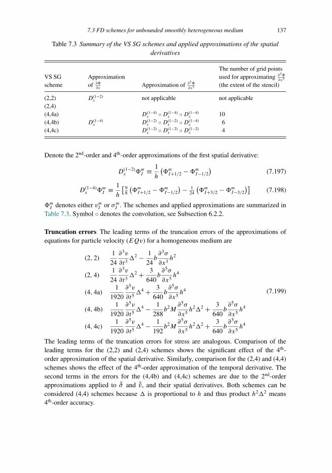
Trim: 247mm × 174mm Top: 14.762mm Gutter: 23.198mmCUUK2497-07 CUUK2497/Moczo ISBN: 978 1 107 02881 4 November 15, 2013 13:36
7.3 FD schemes for unbounded smoothly heterogeneous medium 137
Table 7.3 Summary of the VS SG schemes and applied approximations of the spatialderivatives
VS SGscheme
Approximationof ∂�
∂xApproximation of ∂
3�
∂x3
The number of grid pointsused for approximating ∂3�
∂x3
(the extent of the stencil)
(2,2) D(1−2)x not applicable not applicable
(2,4)(4,4a) D(1−4)
x ◦D(1−4)x ◦D(1−4)
x 10(4,4b) D(1−4)
x D(1−2)x ◦D(1−2)
x ◦D(1−4)x 6
(4,4c) D(1−2)x ◦D(1−2)
x ◦D(1−2)x 4
Denote the 2nd-order and 4th-order approximations of the first spatial derivative:
D(1−2)x �mI ≡ 1
h
(�mI+1/2 −�mI−1/2
)(7.197)
D(1−4)x �mI ≡ 1
h
[98
(�mI+1/2 −�mI−1/2
)− 124
(�mI+3/2 −�mI−3/2
)](7.198)
�mI denotes either vmI or σmI . The schemes and applied approximations are summarized inTable 7.3. Symbol ◦ denotes the convolution, see Subsection 6.2.2.
Truncation errors The leading terms of the truncation errors of the approximations ofequations for particle velocity (EQv) for a homogeneous medium are
(2, 2)1
24
∂3v
∂t3�2 − 1
24b∂3σ
∂x3h2
(2, 4)1
24
∂3v
∂t3�2 + 3
640b∂5σ
∂x5h4
(4, 4a)1
1920
∂5v
∂t5�4 + 3
640b∂5σ
∂x5h4
(4, 4b)1
1920
∂5v
∂t5�4 − 1
288b2M
∂5σ
∂x5h2�2 + 3
640b∂5σ
∂x5h4
(4, 4c)1
1920
∂5v
∂t5�4 − 1
192b2M
∂5σ
∂x5h2�2 + 3
640b∂5σ
∂x5h4
(7.199)
The leading terms of the truncation errors for stress are analogous. Comparison of theleading terms for the (2,2) and (2,4) schemes shows the significant effect of the 4th-order approximation of the spatial derivative. Similarly, comparison for the (2,4) and (4,4)schemes shows the effect of the 4th-order approximation of the temporal derivative. Thesecond terms in the errors for the (4,4b) and (4,4c) schemes are due to the 2nd-orderapproximations applied to ˜σ and ˜v, and their spatial derivatives. Both schemes can beconsidered (4,4) schemes because � is proportional to h and thus product h2�2 means4th-order accuracy.
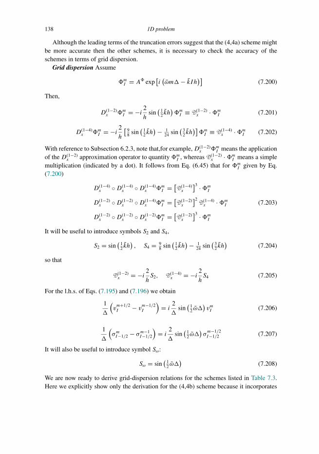
Trim: 247mm × 174mm Top: 14.762mm Gutter: 23.198mmCUUK2497-07 CUUK2497/Moczo ISBN: 978 1 107 02881 4 November 15, 2013 13:36
138 1D problem
Although the leading terms of the truncation errors suggest that the (4,4a) scheme mightbe more accurate then the other schemes, it is necessary to check the accuracy of theschemes in terms of grid dispersion.
Grid dispersion Assume
�mI = A� exp[i(ωm�− kIh)] (7.200)
Then,
D(1−2)x �mI = −i 2
hsin(
12 kh
)�mI ≡ D(1−2)
x ·�mI (7.201)
D(1−4)x �mI = −i 2
h
[98 sin
(12 kh
)− 124 sin
(32 kh
)]�mI ≡ D(1−4)
x ·�mI (7.202)
With reference to Subsection 6.2.3, note that,for example,D(1−2)x �mI means the application
of the D(1−2)x approximation operator to quantity �mI , whereas D(1−2)
x ·�mI means a simplemultiplication (indicated by a dot). It follows from Eq. (6.45) that for �mI given by Eq.(7.200)
D(1−4)x ◦D(1−4)
x ◦D(1−4)x �mI = [
D(1−4)x
]3 ·�mID(1−2)x ◦D(1−2)
x ◦D(1−4)x �mI = [
D(1−2)x
]2 D(1−4)x ·�mI (7.203)
D(1−2)x ◦D(1−2)
x ◦D(1−2)x �mI = [
D(1−2)x
]3 ·�mIIt will be useful to introduce symbols S2 and S4,
S2 = sin(
12 kh
), S4 = 9
8 sin(
12 kh
)− 124 sin
(32 kh
)(7.204)
so that
D(1−2)x = −i 2
hS2, D(1−4)
x = −i 2hS4 (7.205)
For the l.h.s. of Eqs. (7.195) and (7.196) we obtain
1
�
(vm+1/2I − vm−1/2
I
)= i 2
�sin(
12 ω�
)vmI (7.206)
1
�
(σmI−1/2 − σm−1
I−1/2
)= i 2
�sin(
12 ω�
)σm−1/2I−1/2 (7.207)
It will also be useful to introduce symbol Sω:
Sω = sin(
12 ω�
)(7.208)
We are now ready to derive grid-dispersion relations for the schemes listed in Table 7.3.Here we explicitly show only the derivation for the (4,4b) scheme because it incorporates

Trim: 247mm × 174mm Top: 14.762mm Gutter: 23.198mmCUUK2497-07 CUUK2497/Moczo ISBN: 978 1 107 02881 4 November 15, 2013 13:36
7.3 FD schemes for unbounded smoothly heterogeneous medium 139
Table 7.4 Dispersion relations for theVS SG schemes
Scheme Dispersion relation
(2,2) S2S22
(2,4) S2S24
(4,4a) sin2(
12 ω�
) = S2S24
(1 − 1
6S2S2
4
)2
(4,4b) S2S24
(1 − 1
6S2S2
2
)2
(4,4c) S2(S4 − 1
6S2S3
2
)2
both the D(1−2)x and D(1−4)
x approximations. Equations (7.195) and (7.196) may be writtenas
i2
�Sωv
mI = 1
24�2b2M
(−i 2hS2
)2 (−i 2hS4
)σmI + b
(−i 2hS4
)σmI (7.209)
i2
�Sωσ
m−1/2I−1/2 = 1
24�2bM2
(−i 2hS2
)2 (−i 2hS4
)vm−1/2I−1/2 +M
(−i 2hS4
)vm−1/2I−1/2
(7.210)
After rearrangement:
− SωvmI = �
hbS4
(1 − 1
6S2S2
2
)σmI (7.211)
− Sωσm−1/2I−1/2 = �
hMS4
(1 − 1
6S2S2
2
)vm−1/2I−1/2 (7.212)
where, see Eqs. (7.28) and (7.69), S is the Courant number:
S = �
h
√bM = �
hc (7.213)
Substituting m and I for m− 1/2 and I − 1/2, respectively, in Eq. (7.212), we obtain
− SωσmI = �
hMS4
(1 − 1
6S2S2
2
)vmI (7.214)
Multiplying the l.h.s./r.h.s. of Eq. (7.211) by the l.h.s./r.h.s. of Eq. (7.214), respectively, weobtain
S2ω = S2S2
4
(1 − 1
6S2S2
2
)2(7.215)
Equation (7.215) is the grid-dispersion relation for scheme (4,4b). Similarly, we obtainrelations for the other schemes listed in Table 7.3. All are summarized in Table 7.4.

Trim: 247mm × 174mm Top: 14.762mm Gutter: 23.198mmCUUK2497-07 CUUK2497/Moczo ISBN: 978 1 107 02881 4 November 15, 2013 13:36
140 1D problem
0 1 2 3 4-1.0
-0.5
0.0
0.5
1.01.0
0.5
0.0
-0.5
-1.0
S
2S
r.h.s. of the dispersion relation
Figure 7.12 Plot of the r.h.s. of the dispersion relation Eq. (7.216) for −1 ≤ S2 ≤ 1 and 0 ≤ S ≤ 4.
Stability conditions In Subsection 7.2.4 we investigated the stability of scheme (7.21)and found the stability condition S ≤ SM = 1; see Eqs. (7.61)–(7.70). Here we can usethe obtained dispersion relations for finding stability conditions for the investigated VSSG schemes. Consider again the (4,4b) scheme. Equation (7.215) implies, after algebraicmanipulations,
sin(
12 ω�
) = 136SS2
(6 + S2
2
) (6 − S2S2
2
)(7.216)
An important feature of Eq. (7.216) is that the sine function on the r.h.s. appears only withone argument 1
2 kh. Figure 7.12 shows a plot of the r.h.s. of Eq. (7.216) for −1 ≤ S2 ≤ 1and 0 ≤ S ≤ 4. We want to find the minimum value of S above which the l.h.s. of Eq.(7.216) falls outside interval [−1, 1]. It is clear from Fig. 7.12 that the value sought, SM , isobtained from Eq. (7.216) for S2 = 1 or S2 = −1. In both cases we obtain SM = 1.05018.The conclusion for the (4,4b) scheme is that the scheme is stable if
S ≤ SM = 1.05018 (7.217)

Trim: 247mm × 174mm Top: 14.762mm Gutter: 23.198mmCUUK2497-07 CUUK2497/Moczo ISBN: 978 1 107 02881 4 November 15, 2013 13:36
7.3 FD schemes for unbounded smoothly heterogeneous medium 141
Table 7.5 Modified dispersion relations and maximum values SM ofCourant number S for the VS SG schemes
Scheme Modified dispersion relation SM
(2,2) SS2 1.0(2,4) 6−1SS2
(6 + S2
2
)67 ≈ 0.857143
(4,4a) sin(
12 ω�
) = 6−4SS2
(6 + S2
2
) [63 − S2S2
2
(6 + S2
2
)2]
2.44056
(4,4b) 6−2SS2
(6 + S2
2
) (6 − S2S2
2
)1.05018
(4,4c) 6−1SS2
(6 + S2
2 − S2S22
)1.0
or, equivalently,
� ≤ h
cSM = 1.05018
h
c(7.218)
Analogously, we can analyze the other schemes listed in Table 7.3. The modified dispersionrelations and SM values are given in Table 7.5.
The stability conditions for the (2,2) and (2,4) schemes are very well known. The SMvalue for the (4,4c) scheme appears reasonable. The SM values for the (4,4a) and (4,4b)schemes may be surprising because they are larger than 1. This is a consequence of thelarger stencil – the larger number of grid points used for approximating the 3rd spatialderivative.
At this point we recommend additional reading on the analysis of stability and theCourant–Friedrichs–Lewy condition in mathematical books such as those by Strikwerda(2004) and LeVeque (2007).
Normalized grid phase velocity Any of the grid-dispersion relations in Table 7.5 may bewritten as
sin(
12 ω�
) = �(S, kh) (7.219)
from which we have
ω = 2
�arcsin�(S, kh) (7.220)
Assume k = k, that is a grid wave with a true physical wavelength. The grid phase velocity,Eq. (7.19), is
v = ωreal
k= 2
k�arcsin� (S, kh) (7.221)
The normalized grid phase velocity is then
v
c= 2
ck�arcsin� (S, kh) (7.222)
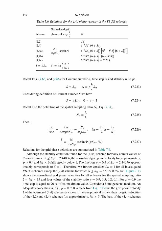
Trim: 247mm × 174mm Top: 14.762mm Gutter: 23.198mmCUUK2497-07 CUUK2497/Moczo ISBN: 978 1 107 02881 4 November 15, 2013 13:36
142 1D problem
Table 7.6 Relations for the grid phase velocity in the VS SG schemes
Scheme
Normalized grid
phase velocityv
c�
(2,2) SS2
(2,4) 6−1SS2
(6 + S2
2
)(4,4a)
Nλ
πpSMarcsin� 6−4SS2
(6 + S2
2
) [63 − S2S2
2
(6 + S2
2
)2]
(4,4b) 6−2SS2
(6 + S2
2
) (6 − S2S2
2
)(4,4c) 6−1SS2
(6 + S2
2 − S2S22
)S = pSM S2 = sin
(π
Nλ
)
Recall Eqs. (7.63) and (7.66) for Courant number S, time step � and stability ratio p:
S ≤ SM, � = phcSM (7.223)
Considering definition of Courant number S we have
S = pSM ; 0 < p ≤ 1 (7.224)
Recall also the definition of the spatial sampling ratio Nλ, Eq. (7.34),
Nλ = λ
h(7.225)
Then,
2
ck�= 2λc
c2πphSM= Nλ
πpSM, kh = 2π
λh = 2π
Nλ(7.226)
v
c= Nλ
πpSMarcsin� (pSM,Nλ) (7.227)
Relations for the grid phase velocities are summarized in Table 7.6.Although the stability condition found for the (4,4a) scheme formally admits values of
Courant number S ≤ SM = 2.44056, the normalized grid phase velocity for, approximately,p > 0.4 and Nλ < 6 falls steeply below 1. The fraction p = 0.4 of SM = 2.44056 approx-imately corresponds to S = 1. Therefore, we further consider SM = 1 for all investigatedVS SG schemes except the (2,4) scheme for which S ≤ SM = 6/7 ≈ 0.857143. Figure 7.13shows the normalized grid phase velocities for all schemes for the spatial sampling ratio2 ≤ Nλ ≤ 15 and four values of the stability ratio p = 0.9, 0.5, 0.2, 0.1. For p = 0.9 thetime step is equal to 90 % of its maximum value. Consider a homogeneous medium. Anadequate choice then is, e.g., p = 0.9. It is clear from Fig. 7.13 that the grid phase velocityv of the optimized (4,4) schemes is closer to the true physical value c than the grid velocitiesof the (2,2) and (2,4) schemes for, approximately, Nλ > 5. The best of the (4,4) schemes
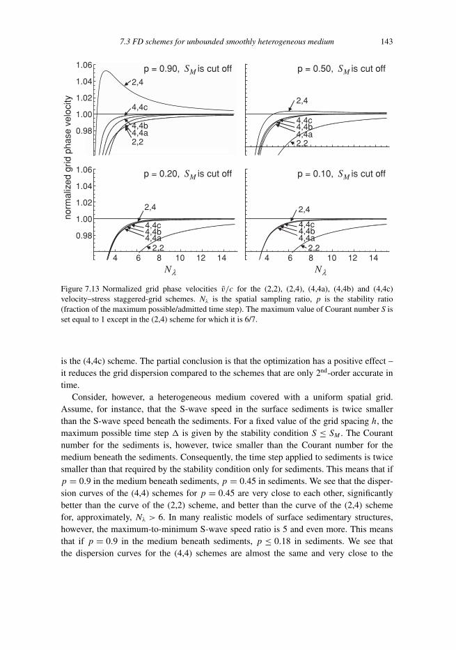
Trim: 247mm × 174mm Top: 14.762mm Gutter: 23.198mmCUUK2497-07 CUUK2497/Moczo ISBN: 978 1 107 02881 4 November 15, 2013 13:36
7.3 FD schemes for unbounded smoothly heterogeneous medium 143
2,4
4,4c
4,4b4,4a2,2
1.06
1.04
1.02
1.00
0.98
cut offMS cut offMS
2,4
4,4c4,4b4,4a2,2
1.06
1.04
1.02
1.00
0.98
2,4
4,4c4,4b4,4a
2,24 6 8 10 12 14
cut offMS
4 6 8 10 12 14
p = 0.90, is p = 0.50, is
p = 0.20, is p = 0.10, is cut offMS
2,4
4,4c4,4b4,4a
2,2
NλNλ
norm
aliz
edgr
idph
ase
velo
city
Figure 7.13 Normalized grid phase velocities v/c for the (2,2), (2,4), (4,4a), (4,4b) and (4,4c)velocity–stress staggered-grid schemes. Nλ is the spatial sampling ratio, p is the stability ratio(fraction of the maximum possible/admitted time step). The maximum value of Courant number S isset equal to 1 except in the (2,4) scheme for which it is 6/7.
is the (4,4c) scheme. The partial conclusion is that the optimization has a positive effect –it reduces the grid dispersion compared to the schemes that are only 2nd-order accurate intime.
Consider, however, a heterogeneous medium covered with a uniform spatial grid.Assume, for instance, that the S-wave speed in the surface sediments is twice smallerthan the S-wave speed beneath the sediments. For a fixed value of the grid spacing h, themaximum possible time step � is given by the stability condition S ≤ SM . The Courantnumber for the sediments is, however, twice smaller than the Courant number for themedium beneath the sediments. Consequently, the time step applied to sediments is twicesmaller than that required by the stability condition only for sediments. This means that ifp = 0.9 in the medium beneath sediments, p = 0.45 in sediments. We see that the disper-sion curves of the (4,4) schemes for p = 0.45 are very close to each other, significantlybetter than the curve of the (2,2) scheme, and better than the curve of the (2,4) schemefor, approximately, Nλ > 6. In many realistic models of surface sedimentary structures,however, the maximum-to-minimum S-wave speed ratio is 5 and even more. This meansthat if p = 0.9 in the medium beneath sediments, p ≤ 0.18 in sediments. We see thatthe dispersion curves for the (4,4) schemes are almost the same and very close to the
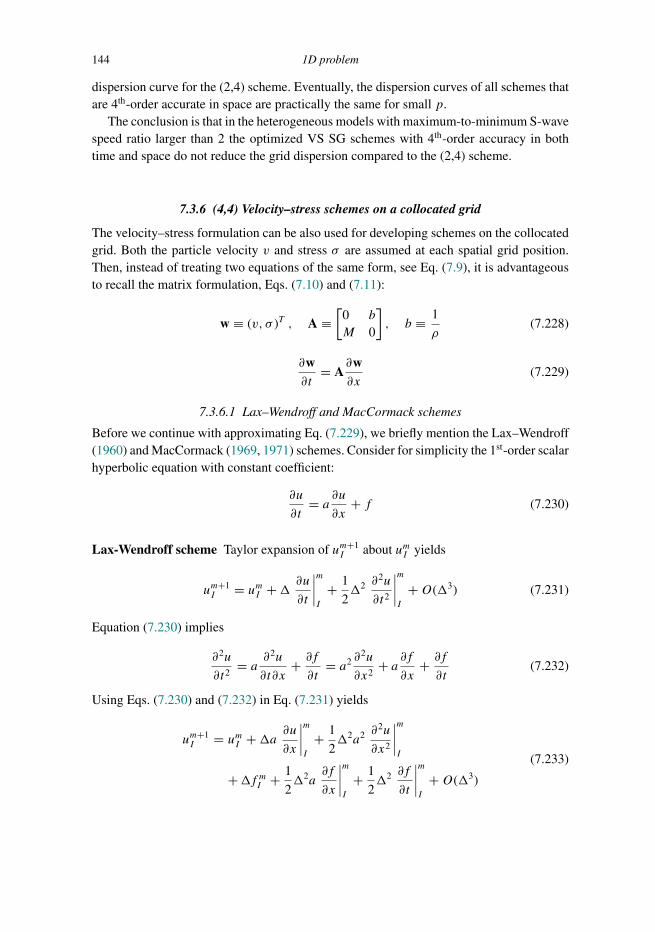
Trim: 247mm × 174mm Top: 14.762mm Gutter: 23.198mmCUUK2497-07 CUUK2497/Moczo ISBN: 978 1 107 02881 4 November 15, 2013 13:36
144 1D problem
dispersion curve for the (2,4) scheme. Eventually, the dispersion curves of all schemes thatare 4th-order accurate in space are practically the same for small p.
The conclusion is that in the heterogeneous models with maximum-to-minimum S-wavespeed ratio larger than 2 the optimized VS SG schemes with 4th-order accuracy in bothtime and space do not reduce the grid dispersion compared to the (2,4) scheme.
7.3.6 (4,4) Velocity–stress schemes on a collocated grid
The velocity–stress formulation can be also used for developing schemes on the collocatedgrid. Both the particle velocity v and stress σ are assumed at each spatial grid position.Then, instead of treating two equations of the same form, see Eq. (7.9), it is advantageousto recall the matrix formulation, Eqs. (7.10) and (7.11):
w ≡ (v, σ )T , A ≡[
0 b
M 0
], b ≡ 1
ρ(7.228)
∂w∂t
= A∂w∂x
(7.229)
7.3.6.1 Lax–Wendroff and MacCormack schemes
Before we continue with approximating Eq. (7.229), we briefly mention the Lax–Wendroff(1960) and MacCormack (1969, 1971) schemes. Consider for simplicity the 1st-order scalarhyperbolic equation with constant coefficient:
∂u
∂t= a ∂u
∂x+ f (7.230)
Lax-Wendroff scheme Taylor expansion of um+1I about umI yields
um+1I = umI +� ∂u
∂t
∣∣∣∣mI
+ 1
2�2 ∂
2u
∂t2
∣∣∣∣mI
+O(�3) (7.231)
Equation (7.230) implies
∂2u
∂t2= a ∂
2u
∂t∂x+ ∂f∂t
= a2 ∂2u
∂x2+ a ∂f
∂x+ ∂f∂t
(7.232)
Using Eqs. (7.230) and (7.232) in Eq. (7.231) yields
um+1I = umI +�a ∂u
∂x
∣∣∣∣mI
+ 1
2�2a2 ∂
2u
∂x2
∣∣∣∣mI
+�fmI + 1
2�2a
∂f
∂x
∣∣∣∣mI
+ 1
2�2 ∂f
∂t
∣∣∣∣mI
+O(�3)
(7.233)

Trim: 247mm × 174mm Top: 14.762mm Gutter: 23.198mmCUUK2497-07 CUUK2497/Moczo ISBN: 978 1 107 02881 4 November 15, 2013 13:36
7.3 FD schemes for unbounded smoothly heterogeneous medium 145
Replacing the spatial derivatives by the 2nd-order centred approximations and ∂f∂t
by theforward approximation we obtain the Lax–Wendroff scheme:
um+1I = umI + �
2ha(umI+1 − umI−1
)+ �2
2h2a2(umI+1 − 2umI + umI−1
)+ �
2
4ha(f mI+1 − f mI−1
)+ �2
(f m+1I + f mI
)+O(�3) +O(h2�)
(7.234)
For stability of the scheme and comparison with other schemes see, e.g., Strikwerda (2004),LeVeque (2007).
MacCormack scheme Consider now the following approximation of Eq. (7.230). First weapply forward approximations of the temporal and spatial derivatives (the latter indicatedby operator DFx ) at time level m and position I :
1
�
(um+1I − umI
) ≈ aDFx umI + f mI (7.235)
Because the approximations are one-sided, the value of u at the time level m+ 1 may beconsidered provisional and therefore denoted by a tilde. Equation (7.235) implies
um+1I ≈ umI +�aDFx umI +�fmI (7.236)
We now approximate Eq. (7.230) in another way. Having the provisional value atm+ 1 wemay apply a backward approximation at this time level. In order to obtain spatial symmetryabout position I , we may apply a backward approximation at this spatial position:
2
�
(um+1I − um+1/2
I
)≈ aDBx um+1
I + f m+1I (7.237)
um+1/2I may be approximated as
um+1/2I ≈ 1
2
(umI + um+1
I
)(7.238)
Equations (7.237) and (7.238) yield
um+1I ≈ 1
2
(umI + um+1
I +�aDBx um+1I +�fm+1
I
)(7.239)
Using relations (7.236) and DBx DFx u
mI = DFx DBx umI in the latter equation we obtain
um+1I ≈ umI + 1
2�a(DFx u
mI +DBx umI
)+ 12�
2a2DBx DFx u
mI
+ 12�f
mI + 1
2�2aDBx f
mI + 1
2�fm+1I
(7.240)
Considering
DFx umI ≡ 1
h
(umI+1 − umI
),DBx u
mI ≡ 1
h
(umI − umI−1
),DBx f
mI ≡ 1
h
(f mI − f mI−1
)(7.241)

Trim: 247mm × 174mm Top: 14.762mm Gutter: 23.198mmCUUK2497-07 CUUK2497/Moczo ISBN: 978 1 107 02881 4 November 15, 2013 13:36
146 1D problem
in Eq. (7.240) we eventually obtain
um+1I = umI + �
2ha(umI+1 − umI−1
)+ �2
2h2a2 (umI+1 − 2umI + umI−1
)+ �
2
(f m+1I + f mI
)+ �2
2ha(f mI − f mI−1
)+O(�3) +O(h2�)(7.242)
Relation between Lax–Wendroff and MacCormack schemes Assuming f = 0, rela-tions (7.234) and (7.242) give the same (2,2) scheme.
7.3.6.2 General relations
We return now to Eq. (7.229); for the following analysis we do not include the force term.Denoting
EQw ≡ ∂w∂t
− A∂w∂x, EQw = 0 (7.243)
we can expressEQw at time levelm and spatial position I , for example, using two or threetime levels. The first option is indicated by 2TL, the second one by 3TL:
2TL : EQw|mI = 1
�
(wm+1I − wmI
)−1
2�∂2w∂t2
∣∣∣∣mI
− 1
6�2 ∂
3w∂t3
∣∣∣∣mI
− 1
24�3 ∂
4w∂t4
∣∣∣∣mI
+O(�4) − A∂w∂x
∣∣∣∣mI
(7.244)
3TL : EQw|mI = 1
2�
(wm+1I − wm−1
I
)− 1
6�2 ∂
3w∂t3
∣∣∣∣mI
+O(�4) − A∂w∂x
∣∣∣∣mI
(7.245)
Replacing the temporal derivatives by spatial derivatives, see Eq. (7.13), we obtain
2TL : EQw|mI = 1
�
(wm+1I − wmI
)− 1
2� A
∂
∂x
(A∂w∂x
)∣∣∣∣mI
− 1
6�2 A
∂
∂x
[A∂
∂x
(A∂w∂x
)]∣∣∣∣mI
− 1
24�3 A
∂
∂x
{A∂
∂x
[A∂
∂x
(A∂w∂x
)]}∣∣∣∣mI
+O(�4) − A∂w∂x
∣∣∣∣mI
(7.246)
3TL : EQw|mI = 1
2�
(wm+1I − wm−1
I
)− 1
6�2 A
∂
∂x
[A∂
∂x
(A∂w∂x
)]∣∣∣∣mI
+O(�4) − A∂w∂x
∣∣∣∣mI
(7.247)
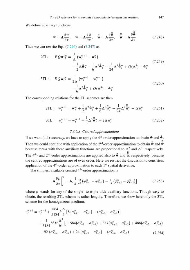
Trim: 247mm × 174mm Top: 14.762mm Gutter: 23.198mmCUUK2497-07 CUUK2497/Moczo ISBN: 978 1 107 02881 4 November 15, 2013 13:36
7.3 FD schemes for unbounded smoothly heterogeneous medium 147
We define auxiliary functions:
w = A∂w∂x, ˜w = A
∂w∂x, ˜w = A
∂ ˜w∂x,
˜w = A
∂ ˜w∂x
(7.248)
Then we can rewrite Eqs. (7.246) and (7.247) as
2TL : EQw|mI = 1
�
(wm+1I − wmI
)− 1
2� ˜wmI − 1
6�2 ˜wmI − 1
24�3 ˜
wmI +O(�4) − wmI
(7.249)
3TL : EQw|mI = 1
2�
(wm+1I − wm−1
I
)− 1
6�2 ˜wmI +O(�4) − wmI
(7.250)
The corresponding relations for the FD schemes are then
2TL : wm+1I = wmI + 1
2�2 ˜wmI + 1
6�3 ˜wmI + 1
24�4 ˜
wmI +�wmI (7.251)
3TL : wm+1I = wm−1
I + 1
3�3 ˜wmI + 2�wmI (7.252)
7.3.6.3 Centred approximations
If we want (4,4) accuracy, we have to apply the 4th-order approximation to obtain w and ˜w.
Then we could continue with application of the 2nd-order approximation to obtain ˜w and˜w
because terms with these auxiliary functions are proportional to �2 and �3, respectively.
The 4th- and 2nd-order approximations are applied also to ˜w and˜w, respectively, because
the centred approximations are of even order. Here we restrict the discussion to consistentapplication of the 4th-order approximation to each 1st spatial derivative.
The simplest available centred 4th-order approximation is
A∂ϕ
∂x
∣∣∣∣mI
= AI1
h
[23
(ϕmI+1 − ϕmI−1
)− 112
(ϕmI+2 − ϕmI−2
)](7.253)
where ϕ stands for any of the single- to triple-tilde auxiliary functions. Though easy toobtain, the resulting 2TL scheme is rather lengthy. Therefore, we show here only the 3TLscheme for the homogeneous medium:
vm+1I = vm−1
I + 864
5184b�
h
[8(σmI+1 − σmI−1
)− (σmI+2 − σmI−2
)]+ 1
5184b2M
�3
h3
[−1584(σmI+1 − σmI−1
)+ 387(σmI+2 − σmI−2
)+ 488(σmI+3 − σmI−3
)− 192
(σmI+4 − σmI−4
)+ 24(σmI+5 − σmI−5
)− (σmI+6 − σmI−6
)](7.254)

Trim: 247mm × 174mm Top: 14.762mm Gutter: 23.198mmCUUK2497-07 CUUK2497/Moczo ISBN: 978 1 107 02881 4 November 15, 2013 13:36
148 1D problem
σm+1I = σm−1
I + 864
5184M�
h
[8(vmI+1 − vmI−1
)− (vmI+2 − vmI−2
)]+ 1
5184bM2�
3
h3
[−1584(vmI+1 − vmI−1
)+ 387(vmI+2 − vmI−2
)+ 488(vmI+3 − vmI−3
)− 192
(vmI+4 − vmI−4
)+ 24(vmI+5 − vmI−5
)− (vmI+6 − vmI−6
)](7.255)
We can see an interesting result. vm+1I depends on vm−1
I and σmI±k; k = 1, . . . , 6. σm+1I
depends on σm−1I and vmI±k; k = 1, . . . , 6. This means that, although we have both vm+1
I
and σm+1I at the same space–time grid point, formally vm+1
I does not know about σm+1I and
vice versa. Moreover, the odd-indexed and even-indexed time levels of the particle velocityare separated (decoupled). The same is true of the stresses. This is known as temporalodd–even decoupling.
In the case of the 2TL scheme, vm+1I depends on vmI±k; k = 0, . . . , 8 and σmI±k; k =
1, . . . , 6. Similarly, σm+1I depends on σmI±k; k = 0, . . . , 8 and vmI±k; k = 1, . . . , 6. In other
words, contrary to the 3TL scheme, vm+1I and σm+1
I are not independent.Both schemes have, however, one more important property. Consider first the 2TL
scheme. Assume the following initial conditions:
v0I = 0, σ 0
2k+1 = σODD, σ 02k = σEVEN, k = 0,±1,±2, . . . (7.256)
that is, zero velocity everywhere, σODD at the odd-indexed spatial positions and σEVEN atthe even-indexed spatial positions. The 2TL scheme gives
vmI = 0, σm2k+1 = σODD, σm2k = σEVEN, k = 0,±1,±2, . . . (7.257)
The scheme simply reproduces the initial values.In the case of the 3TL schemes (7.254) and (7.255), we can restrict the treatment to one
of the two independent schemes. Assume the following initial conditions:
v0I = 0, σ 1
2k+1 = σODD, σ 12k = σEVEN, k = 0,±1,±2, . . . (7.258)
The scheme gives
v2mI = 0, σ 2m+1
2k+1 = σODD, σ 2m+12k = σEVEN, k = 0,±1,±2, . . . (7.259)
The scheme reproduces the initial values.The phenomenon observed in both the 2TL and 3TL schemes is known as spatial
odd–even decoupling. The spatial decoupling is due to the application of the centredapproximation to the first spatial derivative. Similarly, the temporal decoupling is due tothe application of the centred approximation to the first temporal derivative.
The property of odd–even decoupling is general – it arises if the 1st derivatives in the1st-order hyperbolic equations are replaced by centred approximations on the collocatedgrids.

Trim: 247mm × 174mm Top: 14.762mm Gutter: 23.198mmCUUK2497-07 CUUK2497/Moczo ISBN: 978 1 107 02881 4 November 15, 2013 13:36
7.3 FD schemes for unbounded smoothly heterogeneous medium 149
7.3.6.4 Noncentred approximations
It is obvious that we can avoid temporal odd–even decoupling by using the 2TL approach,and spatial odd–even decoupling by using a noncentred approximation of the first spatialderivative.
Define the 4th-order forward and backward operators:
DFx [ϕI ] = 1
h
∑3
j=−1cjϕI+j , DBx [ϕI ] = 1
h
∑3
j=−1−cjϕI−j (7.260)
with coefficients
c−1 = −1
4, c0 = −5
6, c1 = 3
2, c2 = −1
2, c3 = 1
12(7.261)
Then,
A∂ϕ
∂x
∣∣∣∣FI
≈ AIDFx [ϕI ] , A∂ϕ
∂x
∣∣∣∣BI
≈ AIDBx [ϕI ] (7.262)
Define auxiliary quantities:F wmI = AIDFx
[wmI], BwmI = AIDBx
[wmI]
B ˜wmI = AIDBx[F wmI
], F ˜wmI = AIDFx
[BwmI
]F ˜wmI = AIDFx
[B ˜wmI
], B ˜wmI = AIDBx
[F ˜wmI
]B ˜
wmI = AIDBx[F ˜wmI
], F ˜
wmI = AIDFx[B ˜wmI
](7.263)
Equation (7.251) then can be written as
wm+1I = wmI +�1
2
(F wmI + BwmI
)+ 1
2�2 1
2
(B ˜wmI + F ˜wmI
)+ 1
6�3 1
2
(F ˜wmI + B ˜wmI
)+ 1
24�4 1
2
(B ˜
wmI + F ˜wmI) (7.264)
In the homogeneous medium the resulting scheme for the particle velocity is
vm+1I = vmI + 1
497664
{6
(−135360bM
�2
h2+ 60265b2M2�
4
h4
)vmI
+ b�h
[435456
(σmI+1 − σmI−1
)− 124416(σmI+2 − σmI−2
)+ 20736(σmI+3 − σmI−3
)]+ bM�
2
h2
[456192
(vmI+1 + vmI−1
)− 41472(vmI+2 + vmI−2
)− 13824(vmI+3 + vmI−3
)+ 5184
(vmI+4 + vmI−4
)]+ b2M�3
h3
[−264600(σmI+1 − σmI−1
)+ 211536
(σmI+2 − σmI−2
)− 62904(σmI+3 − σmI−3
)+ 5760(σmI+4 − σmI−4
)+ 2088
(σmI+5 − σmI−5
)− 624(σmI+6 − σmI−6
)+ 72(σmI+7 − σmI−7
)]+ b2M2�
4
h4
[−260496(vmI+1 + vmI−1
)+ 87888(vmI+2 + vmI−2
)− 3568
(vmI+3 + vmI−3
)− 6468(vmI+4 + vmI−4
)+ 1968(vmI+5 + vmI−5
)− 80
(vmI+6 + vmI−6
)− 48(vmI+7 + vmI−7
)+ 9(vmI+8 + vmI−8
)]}
(7.265)
The scheme for the stress is analogous.
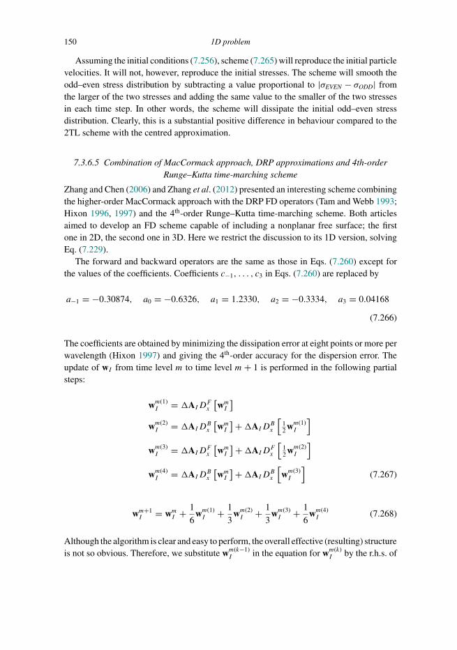
Trim: 247mm × 174mm Top: 14.762mm Gutter: 23.198mmCUUK2497-07 CUUK2497/Moczo ISBN: 978 1 107 02881 4 November 15, 2013 13:36
150 1D problem
Assuming the initial conditions (7.256), scheme (7.265) will reproduce the initial particlevelocities. It will not, however, reproduce the initial stresses. The scheme will smooth theodd–even stress distribution by subtracting a value proportional to |σEVEN − σODD| fromthe larger of the two stresses and adding the same value to the smaller of the two stressesin each time step. In other words, the scheme will dissipate the initial odd–even stressdistribution. Clearly, this is a substantial positive difference in behaviour compared to the2TL scheme with the centred approximation.
7.3.6.5 Combination of MacCormack approach, DRP approximations and 4th-orderRunge–Kutta time-marching scheme
Zhang and Chen (2006) and Zhang et al. (2012) presented an interesting scheme combiningthe higher-order MacCormack approach with the DRP FD operators (Tam and Webb 1993;Hixon 1996, 1997) and the 4th-order Runge–Kutta time-marching scheme. Both articlesaimed to develop an FD scheme capable of including a nonplanar free surface; the firstone in 2D, the second one in 3D. Here we restrict the discussion to its 1D version, solvingEq. (7.229).
The forward and backward operators are the same as those in Eqs. (7.260) except forthe values of the coefficients. Coefficients c−1, . . . , c3 in Eqs. (7.260) are replaced by
a−1 = −0.30874, a0 = −0.6326, a1 = 1.2330, a2 = −0.3334, a3 = 0.04168
(7.266)
The coefficients are obtained by minimizing the dissipation error at eight points or more perwavelength (Hixon 1997) and giving the 4th-order accuracy for the dispersion error. Theupdate of wI from time level m to time level m+ 1 is performed in the following partialsteps:
wm(1)I = �AIDFx
[wmI]
wm(2)I = �AIDBx
[wmI]+�AIDBx
[12 wm(1)
I
]wm(3)I = �AIDFx
[wmI]+�AIDFx
[12 wm(2)
I
]wm(4)I = �AIDBx
[wmI]+�AIDBx
[wm(3)I
](7.267)
wm+1I = wmI + 1
6wm(1)I + 1
3wm(2)I + 1
3wm(3)I + 1
6wm(4)I (7.268)
Although the algorithm is clear and easy to perform, the overall effective (resulting) structureis not so obvious. Therefore, we substitute wm(k−1)
I in the equation for wm(k)I by the r.h.s. of

Trim: 247mm × 174mm Top: 14.762mm Gutter: 23.198mmCUUK2497-07 CUUK2497/Moczo ISBN: 978 1 107 02881 4 November 15, 2013 13:36
7.4 FD schemes for a material interface 151
the equation for wm(k−1)I . Eventually we obtain
wm+1I = wmI +�
{1
2AIDFx
[wmI]+ 1
2AIDBx
[wmI]}
+�2 1
2
⎧⎪⎪⎪⎪⎨⎪⎪⎪⎪⎩
1
3AIDBx
[AIDFx
[wmI]]
+1
3AIDFx
[AIDBx
[wmI]]
+1
3AIDBx
[AIDFx
[wmI]]
⎫⎪⎪⎪⎪⎬⎪⎪⎪⎪⎭
+�3 1
6
⎧⎪⎨⎪⎩
1
2AIDFx
[AIDBx
[AIDFx
[wmI]]]
+1
2AIDBx
[AIDFx
[AIDBx
[wmI]]]⎫⎪⎬⎪⎭
+�4 1
24
{AIDBx
[AIDFx
[AIDBx
[AIDFx
[wmI]]]]}
(7.269)
It is clear that the expressions in the four braces are approximations to
A∂w∂x,A∂
∂x
(A∂w∂x
),A∂
∂x
[A∂
∂x
(A∂w∂x
)],A∂
∂x
{A∂
∂x
[A∂
∂x
(A∂w∂x
)]}(7.270)
at (I,m), respectively. Comparison with Eqs. (7.246) and (7.251) shows that scheme (7.267)and (7.268) can be obtained by the Lax–Wendroff approach applied to Eq. (7.229) andaiming to develop the (4,4) velocity–stress scheme on the collocated grid using two timelevels. Consequently, the difference between scheme (7.267)–(7.268) and scheme (7.263)–(7.264) is in the method of approximating the four terms (7.270).
7.4 FD schemes for a material interface
In Section 7.2 we assumed an unbounded homogeneous medium in which both the elasticmodulus and density are spatial constants. In Section 7.3 we assumed a smoothly hetero-geneous medium. Comparison of the strong-form formulations indicates why we explicitlyaddressed the question of determining the effective grid modulus (MI ) only in Subsection7.3.1, where we presented the (2,2) displacement scheme on a conventional grid. We hadto treat the term ∂ (M∂u/∂x)/∂x in the displacement formulation, Eq. (7.2). We used amathematical trick to avoid differentiating the modulus. The other strong-form formula-tions did not force us to treat the determination of the grid modulus explicitly. We simplyindicated the effective grid modulus assigned to a grid spatial position by a correspondingspatial subscript. The same applies to density ρ or its reciprocal value b for all strong-formformulations.
Although the smoothness of the heterogeneous medium is a mathematically clear con-cept, it is obvious that two smooth media can differ from each other by gradient. Loosely,we can guess that local values of modulus and density at a spatial grid position might besufficient in the case of small gradients. On the other hand, we may have some doubts

Trim: 247mm × 174mm Top: 14.762mm Gutter: 23.198mmCUUK2497-07 CUUK2497/Moczo ISBN: 978 1 107 02881 4 November 15, 2013 13:36
152 1D problem
about using the local values in the case of large gradients. What is a small and what is alarge value of a gradient is, of course, relative. In general, appropriate measures of spatialvariability of the medium should be compared with the wavelengths or frequencies thatare to be sufficiently accurately propagated in the grid. Consequently, the determination ofoptimal values of modulus and density at a grid position is not a trivial problem.
Probably the most important type of spatial variability of a material parameter is itsdiscontinuous change – in other words, a material discontinuity or a material interface.
7.4.1 Simple general consideration
We start with a simple general consideration. Let ϕ− (x), K− (x) and ψ− (x) be realfunctions of a real argument x < 0. Similarly, let ϕ+ (x), K+ (x) and ψ+ (x) be realfunctions of a real argument x > 0. Assume that the functions have their limits at x = 0,which we denote by ϕ−(0), K−(0), ψ−(0), ϕ+(0), K+(0) and ψ+(0), respectively. Thefunctions satisfy equations
ϕ− (x) = K− (x)ψ− (x) , ϕ+ (x) = K+ (x)ψ+ (x) (7.271)
Moreover, functions ϕ± (x) satisfy the boundary (continuity) condition
ϕ(0) = ϕ−(0) = ϕ+(0) (7.272)
Due to the boundary condition, neither of Eqs. (7.271) alone can be used as an equation forx = 0.
Define
ψA(0) ≡ 12
[ψ−(0) + ψ+(0)
](7.273)
Then,
ψA(0) = 1
2
[ϕ−(0)
K−(0)+ ϕ+(0)
K+(0)
]= 1
2ϕ(0)
[1
K−(0)+ 1
K+(0)
](7.274)
Define
KH (0) ≡ 2[1
K−(0) + 1
K+(0)
] (7.275)
Then,
ϕ(0) = KH (0)ψA(0) (7.276)
Equation (7.276) has two important properties: (1) it is valid directly at x = 0, (2) it hasthe same form as each of Eqs. (7.271). This is due to the arithmetic averaging of ψ−(0)and ψ+(0), and the harmonic averaging of K−(0) and K+(0). Note that the arithmetic andharmonic averages are indicated by superscripts A and H starting with Eqs. (7.273) and(7.275).
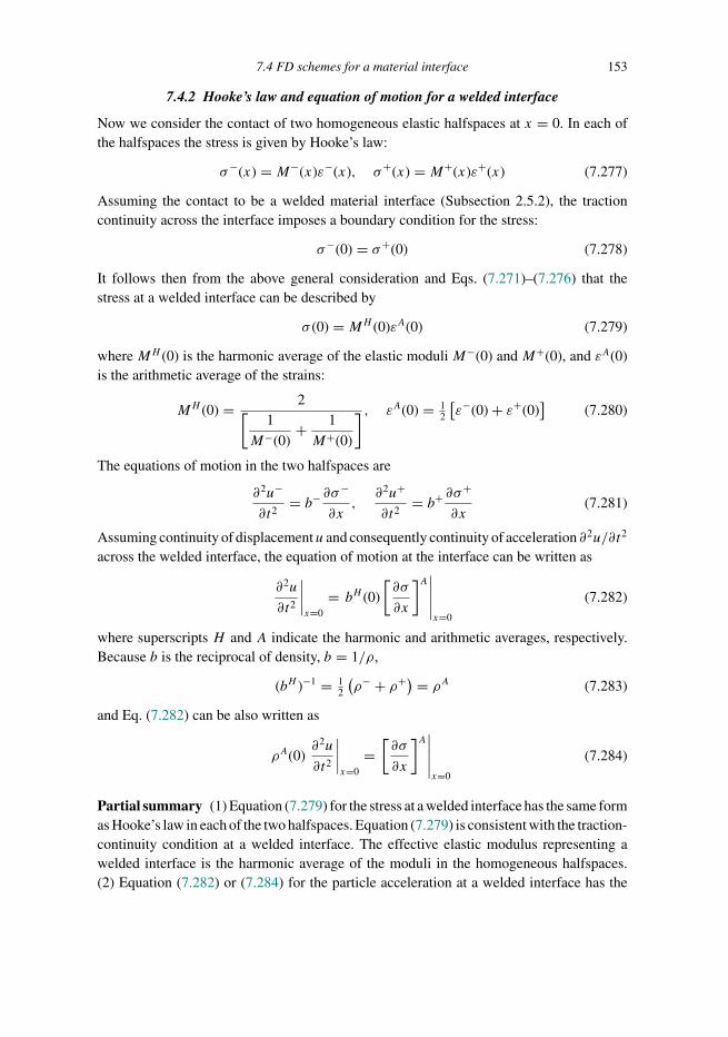
Trim: 247mm × 174mm Top: 14.762mm Gutter: 23.198mmCUUK2497-07 CUUK2497/Moczo ISBN: 978 1 107 02881 4 November 15, 2013 13:36
7.4 FD schemes for a material interface 153
7.4.2 Hooke’s law and equation of motion for a welded interface
Now we consider the contact of two homogeneous elastic halfspaces at x = 0. In each ofthe halfspaces the stress is given by Hooke’s law:
σ−(x) = M−(x)ε−(x), σ+(x) = M+(x)ε+(x) (7.277)
Assuming the contact to be a welded material interface (Subsection 2.5.2), the tractioncontinuity across the interface imposes a boundary condition for the stress:
σ−(0) = σ+(0) (7.278)
It follows then from the above general consideration and Eqs. (7.271)–(7.276) that thestress at a welded interface can be described by
σ (0) = MH (0)εA(0) (7.279)
whereMH (0) is the harmonic average of the elastic moduliM−(0) andM+(0), and εA(0)is the arithmetic average of the strains:
MH (0) = 2[1
M−(0)+ 1
M+(0)
] , εA(0) = 12
[ε−(0) + ε+(0)
](7.280)
The equations of motion in the two halfspaces are
∂2u−
∂t2= b− ∂σ
−
∂x,∂2u+
∂t2= b+ ∂σ
+
∂x(7.281)
Assuming continuity of displacementu and consequently continuity of acceleration ∂2u/∂t2
across the welded interface, the equation of motion at the interface can be written as
∂2u
∂t2
∣∣∣∣x=0
= bH (0)
[∂σ
∂x
]A∣∣∣∣∣x=0
(7.282)
where superscripts H and A indicate the harmonic and arithmetic averages, respectively.Because b is the reciprocal of density, b = 1/ρ,
(bH )−1 = 12
(ρ− + ρ+) = ρA (7.283)
and Eq. (7.282) can be also written as
ρA(0)∂2u
∂t2
∣∣∣∣x=0
=[∂σ
∂x
]A∣∣∣∣∣x=0
(7.284)
Partial summary (1) Equation (7.279) for the stress at a welded interface has the same formas Hooke’s law in each of the two halfspaces. Equation (7.279) is consistent with the traction-continuity condition at a welded interface. The effective elastic modulus representing awelded interface is the harmonic average of the moduli in the homogeneous halfspaces.(2) Equation (7.282) or (7.284) for the particle acceleration at a welded interface has the

Trim: 247mm × 174mm Top: 14.762mm Gutter: 23.198mmCUUK2497-07 CUUK2497/Moczo ISBN: 978 1 107 02881 4 November 15, 2013 13:36
154 1D problem
same form as the equation of motion in each of the two halfspaces. Equation (7.282)or (7.284) is consistent with the condition of continuity of displacement and particleacceleration at a welded interface. The effective density representing a welded interfaceis the arithmetic average of densities in the halfspaces. The statements make an importantbasis for developing an FD scheme for the grid point at the interface and grid points in thehalfspaces.
7.4.3 Simple rheological model of a welded interface
Before we continue with an FD scheme we can recall the simple rheological model of twoHooke elements (elastic springs) connected in series, see Chapter 3. The resulting stress isequal to the stresses acting on the springs:
σ = σ− = σ+ (7.285)
whereas the strains of the springs are additive:
ε = ε− + ε+ = σ
M− + σ
M+ (7.286)
We can think of finding an averaged Hooke spring such that the serial connection of twoaveraged springs would make an equivalent, in terms of the resulting stress and strain, to theconsidered serial connection of two different springs. We easily find the averaged spring:
σ = MHεA, MH = 2[1
M− + 1
M+
] , εA = 1
2
(ε− + ε+) (7.287)
This means that the elastic modulus of the averaged spring is the harmonic average ofthe elastic moduli of the two springs. The serial connection of two springs can be thusconsidered a rheological model for traction continuity at the welded interface of twohomogeneous halfspaces.
Similarly, we could consider a system of two connected particles with masses m− andm+. If the particles move together, the equivalent system can be made of two identicalparticles with mass equal to the arithmetic average of masses m− and m+.
7.4.4 FD schemes
Equations (7.279) and (7.284) suggest (a) harmonic averaging of the elastic moduli andarithmetic averaging of the densities at the material discontinuity, (b) averaging of thespatial derivatives of the functions at the material discontinuity.
The averaging of derivatives means averaging one-sided approximations of the deriva-tives of stresses and strains (or displacement). In 1D this poses a minor algorithmicalproblem. Having in mind the perspective of 2D or 3D simulations for a medium withnonplanar interfaces, it is clear that calculations of one-sided derivatives pose a morecomplicated problem. Moreover, it is not trivial to test the accuracy of such an approach.

Trim: 247mm × 174mm Top: 14.762mm Gutter: 23.198mmCUUK2497-07 CUUK2497/Moczo ISBN: 978 1 107 02881 4 November 15, 2013 13:36
7.5 FD schemes for a free surface 155
Kristek and Moczo (2006) neglected averaging of the spatial derivatives at the interface.They defined the effective grid modulus and density as
MHI+1/2 ≡
[1
h
∫ xI+1
xI
1
M(x)dx
]−1
, ρAI ≡[
1
h
∫ xI+1/2
xI−1/2
ρ(x)dx
](7.288)
They applied these effective grid material parameters to three 1D schemes – (2,2) displace-ment scheme on the conventional grid, (2,4) displacement–stress scheme on the spatiallystaggered grid, and displacement optimally accurate scheme on the conventional grid. Theyperformed detailed numerical tests of the three schemes for an unbounded homogeneousspace, two halfspaces in welded contact, and for a model of an interior layer between twohalfspaces. The interior layer had a large velocity gradient. The model of an unboundedhomogeneous space enabled them to compare the pure effect of grid dispersion. The sim-ulations for the model with a material interface were designed so that it was possible toseparate the error due to the interface. The third model enabled them to compare the capa-bility of the schemes to account for a dramatic change of velocity inside the layer betweentwo identical halfspaces.
All simulations obtained with the FD schemes were compared with analytical matrixsolutions. The level of accuracy of the FD solutions was quantified and characterized usingenvelope and phase misfits with respect to the analytical solutions.
For all three schemes and models, Kristek and Moczo (2006) demonstrated the superioraccuracy of harmonic averaging of the elastic modulus compared to considering localvalues or arithmetic averaging of the elastic modulus. Also relevant for this chapter is theconclusion that the optimally accurate scheme is significantly more accurate than the twoother schemes tested.
It is obvious that neglecting the averaging of the spatial derivatives of stress and straindecreases the order of accuracy of the scheme across the interface. Moczo et al. (2007a,Chapter 10) compared the conventional and optimally accurate schemes (1st-order accurateat the interface) with conventional and optimally accurate schemes treating the interfaceexplicitly (and thus 2nd-order accurate at the interface). As might be expected, the applica-tion of the latter schemes increased accuracy at the interface.
In conclusion, all the FD schemes presented so far can be used with the effective gridparameters defined by Eqs. (7.288). The use of harmonic averaging of the elastic modulusin smoothly and discontinuously heterogeneous media makes an FD scheme capable ofsufficiently accurately accounting for the medium heterogeneity. Specifically, it makes thescheme capable of sensing the position of the material interface within one grid spacing,that is, anywhere between two neighbouring spatial grid points.
7.5 FD schemes for a free surface
Two aspects make the Earth’s surface a very important structural feature that has to bemodelled sufficiently accurately: (a) seismic motion is often recorded at or close to theEarth’s surface; (b) the Earth’s surface significantly affects seismic wave propagation and

Trim: 247mm × 174mm Top: 14.762mm Gutter: 23.198mmCUUK2497-07 CUUK2497/Moczo ISBN: 978 1 107 02881 4 November 15, 2013 13:36
156 1D problem
earthquake motion. In most seismological applications, the air/fluid (ocean) or air/solid(land) interface can be thought of as a free surface where a fluid or solid discontinuouslyterminates and air is replaced by vacuum. This means that the Earth’s surface may beapproximated by a surface with vanishing traction.
Consider a free surface at x = 0 and medium at x ≥ 0. The traction-free condition (2.39)reduces in 1D to
σ (x = 0) = 0 (7.289)
No matter which FD scheme is used, it is desirable to locate the grid position of displacementor particle velocity at the free surface. We restrict our considerations here to the velocity–stress schemes, although many of the explained approaches can also be applied to thedisplacement–stress or displacement schemes. In the case of a staggered grid the stress islocated inside the medium – a half-grid spacing away from the free surface. In the case ofa conventional grid the stress is also located at the free surface.
We have two principal possibilities for calculating particle velocity at the free surface,and particle velocity and stress inside the medium near the free surface. The first approach:apply the same FD schemes as for the interior grid points assuming virtual values of stress,particle velocity and material parameters outside the medium. The second approach: applyone-sided schemes that do not need any virtual values outside the medium.
The advantage of the first approach is the use of one and the same scheme at anygrid point. Its disadvantage is the need to reasonably define virtual values outside themedium. The disadvantage of the second approach is the application of different schemesfor different grid positions inside the medium near the free surface – the number of gridpositions depends on the scheme and the order of approximation.
The first approach leads to the so-called vacuum formalism (zero modulus outside themedium), medium taper (density taper) or imaging method. In this 1D introduction weoutline only the imaging method suggested by Levander (1988). The second approach willbe illustrated by the adjusted FD approximations suggested by Kristek et al. (2002).
7.5.1 Stress imaging
The basic idea in 1D is very simple: the antisymmetry
σ (−x) = −σ (x) (7.290)
ensures that the boundary condition given by Eq. (7.289) is satisfied. Recall the (2,4)velocity–stress staggered-grid scheme (7.186) with the spatial index I + 1/2 for stress:
Vm+1/2I = V m−1/2
I + bI �h
[9
8
(T mI+1/2 − T mI−1/2
)− 1
24
(T mI+3/2 − T mI−3/2
)]
T mI+1/2 = T m−1I+1/2 +MI+1/2
�
h
[9
8
(Vm−1/2I+1 − V m−1/2
I
)− 1
24
(Vm−1/2I+2 − V m−1/2
I−1
)](7.291)
We assume the effective grid material parameters calculated according to (7.288).
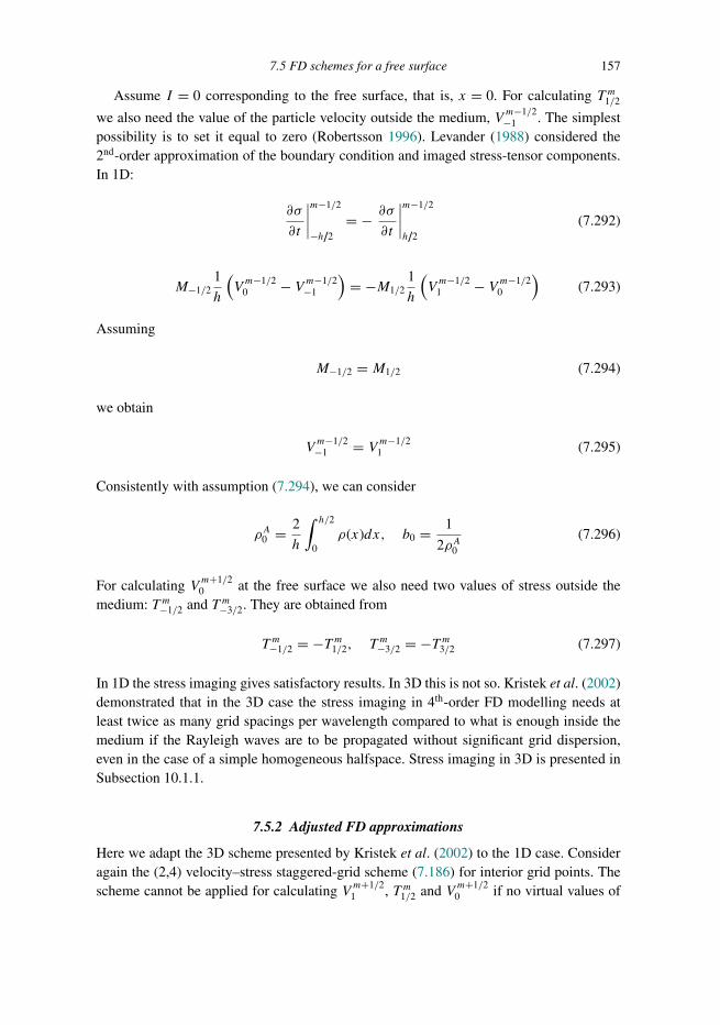
Trim: 247mm × 174mm Top: 14.762mm Gutter: 23.198mmCUUK2497-07 CUUK2497/Moczo ISBN: 978 1 107 02881 4 November 15, 2013 13:36
7.5 FD schemes for a free surface 157
Assume I = 0 corresponding to the free surface, that is, x = 0. For calculating T m1/2we also need the value of the particle velocity outside the medium, V m−1/2
−1 . The simplestpossibility is to set it equal to zero (Robertsson 1996). Levander (1988) considered the2nd-order approximation of the boundary condition and imaged stress-tensor components.In 1D:
∂σ
∂t
∣∣∣∣m−1/2
−h/2
= − ∂σ
∂t
∣∣∣∣m−1/2
h/2
(7.292)
M−1/21
h
(Vm−1/2
0 − V m−1/2−1
)= −M1/2
1
h
(Vm−1/2
1 − V m−1/20
)(7.293)
Assuming
M−1/2 = M1/2 (7.294)
we obtain
Vm−1/2−1 = V m−1/2
1 (7.295)
Consistently with assumption (7.294), we can consider
ρA0 = 2
h
∫ h/2
0ρ(x)dx, b0 = 1
2ρA0(7.296)
For calculating V m+1/20 at the free surface we also need two values of stress outside the
medium: T m−1/2 and T m−3/2. They are obtained from
T m−1/2 = −T m1/2, T m−3/2 = −T m3/2 (7.297)
In 1D the stress imaging gives satisfactory results. In 3D this is not so. Kristek et al. (2002)demonstrated that in the 3D case the stress imaging in 4th-order FD modelling needs atleast twice as many grid spacings per wavelength compared to what is enough inside themedium if the Rayleigh waves are to be propagated without significant grid dispersion,even in the case of a simple homogeneous halfspace. Stress imaging in 3D is presented inSubsection 10.1.1.
7.5.2 Adjusted FD approximations
Here we adapt the 3D scheme presented by Kristek et al. (2002) to the 1D case. Consideragain the (2,4) velocity–stress staggered-grid scheme (7.186) for interior grid points. Thescheme cannot be applied for calculating V m+1/2
1 , T m1/2 and V m+1/20 if no virtual values of
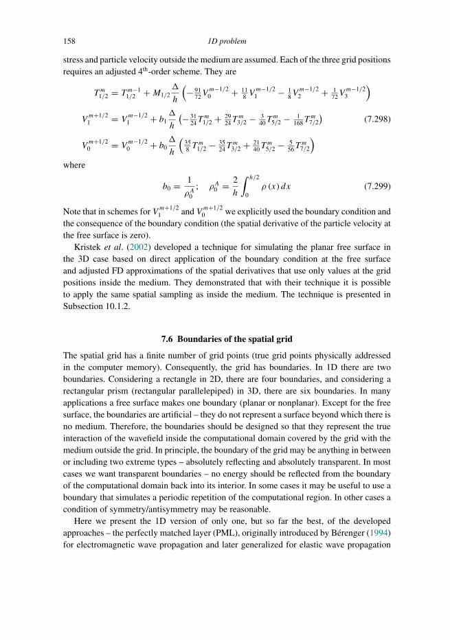
Trim: 247mm × 174mm Top: 14.762mm Gutter: 23.198mmCUUK2497-07 CUUK2497/Moczo ISBN: 978 1 107 02881 4 November 15, 2013 13:36
158 1D problem
stress and particle velocity outside the medium are assumed. Each of the three grid positionsrequires an adjusted 4th-order scheme. They are
T m1/2 = T m−11/2 +M1/2
�
h
(− 91
72Vm−1/2
0 + 118 V
m−1/21 − 1
8Vm−1/2
2 + 172V
m−1/23
)Vm+1/2
1 = V m−1/21 + b1
�
h
(− 3124T
m1/2 + 29
24Tm
3/2 − 340T
m5/2 − 1
168Tm
7/2
)(7.298)
Vm+1/2
0 = V m−1/20 + b0
�
h
(358 T
m1/2 − 35
24Tm
3/2 + 2140T
m5/2 − 5
56Tm
7/2
)where
b0 = 1
ρA0; ρA0 = 2
h
∫ h/2
0ρ (x) dx (7.299)
Note that in schemes for V m+1/21 and V m+1/2
0 we explicitly used the boundary condition andthe consequence of the boundary condition (the spatial derivative of the particle velocity atthe free surface is zero).
Kristek et al. (2002) developed a technique for simulating the planar free surface inthe 3D case based on direct application of the boundary condition at the free surfaceand adjusted FD approximations of the spatial derivatives that use only values at the gridpositions inside the medium. They demonstrated that with their technique it is possibleto apply the same spatial sampling as inside the medium. The technique is presented inSubsection 10.1.2.
7.6 Boundaries of the spatial grid
The spatial grid has a finite number of grid points (true grid points physically addressedin the computer memory). Consequently, the grid has boundaries. In 1D there are twoboundaries. Considering a rectangle in 2D, there are four boundaries, and considering arectangular prism (rectangular parallelepiped) in 3D, there are six boundaries. In manyapplications a free surface makes one boundary (planar or nonplanar). Except for the freesurface, the boundaries are artificial – they do not represent a surface beyond which there isno medium. Therefore, the boundaries should be designed so that they represent the trueinteraction of the wavefield inside the computational domain covered by the grid with themedium outside the grid. In principle, the boundary of the grid may be anything in betweenor including two extreme types – absolutely reflecting and absolutely transparent. In mostcases we want transparent boundaries – no energy should be reflected from the boundaryof the computational domain back into its interior. In some cases it may be useful to use aboundary that simulates a periodic repetition of the computational region. In other cases acondition of symmetry/antisymmetry may be reasonable.
Here we present the 1D version of only one, but so far the best, of the developedapproaches – the perfectly matched layer (PML), originally introduced by Berenger (1994)for electromagnetic wave propagation and later generalized for elastic wave propagation

Trim: 247mm × 174mm Top: 14.762mm Gutter: 23.198mmCUUK2497-07 CUUK2497/Moczo ISBN: 978 1 107 02881 4 November 15, 2013 13:36
7.6 Boundaries of the spatial grid 159
by Chew and Liu (1996) and others. The name comes from the fact that the PML in a truecontinuum space does not reflect energy back to the computational domain. In 2D or 3D thePML makes a ‘sponge’ region surrounding the computational domain. Inside a PML theparticle velocity and stress are attenuated in the direction perpendicular to the boundary.In 1D a PML reduces to a spatial range of grid points at the ‘end’ of the computational1D domain. Here we adapt the 3D theory presented by Komatitsch and Martin (2007) andKristek et al. (2009).
7.6.1 Perfectly matched layer: theory
Application of the Fourier transform to Eqs. (7.9) yields
iωv = b∂σ∂x, iωσ = M ∂v
∂x(7.300)
Here we use the same symbols for the quantities in the frequency and time domains. Also,we indicate the time or frequency as variables just to emphasize them. We replace thespatial differentiation with respect to x by the spatial differentiation with respect to x:
∂
∂x= 1
s
∂
∂x(7.301)
Here s is the stretching factor (or coordinate stretching variable):
s = γ + �
α + iω(7.302)
where γ , � and α are, in general, functions of x and define the PML medium profile. Thestretching factor has to be complex if it is to attenuate. Equations (7.300) then become
iωv = 1
γb∂σ
∂x− d
a + iωb∂σ
∂x, iωσ = 1
γM∂v
∂x− d
a + iωM∂v
∂x(7.303)
with
a = α +�/γ , d = �/γ 2 (7.304)
Because the second term on the r.h.s. of each of Eqs. (7.303) is a product of two complexquantities, an application of the inverse Fourier transform to the equations would give thetime-domain equations with convolutory terms. In order to avoid the convolution, we defineauxiliary functions:
θ (ω) = − d
a + iωb∂σ
∂x, ζ (ω) = − d
a + iωM∂v
∂x(7.305)
Equations (7.303) then become
iωv = 1
γb∂σ
∂x+ θ (ω) , iωσ = 1
γM∂v
∂x+ ζ (ω) (7.306)

Trim: 247mm × 174mm Top: 14.762mm Gutter: 23.198mmCUUK2497-07 CUUK2497/Moczo ISBN: 978 1 107 02881 4 November 15, 2013 13:36
160 1D problem
Application of the inverse Fourier transform to the latter equations gives
∂v
∂t= 1
γb∂σ
∂x+ θ (t) ,
∂σ
∂t= 1
γM∂v
∂x+ ζ (t) (7.307)
In order to find relations for θ (t) and ζ (t), we rewrite Eqs. (7.305):
aθ (ω) + iωθ (ω) = −db∂σ∂x, aζ (ω) + iωζ (ω) = −dM ∂v
∂x(7.308)
and apply the inverse Fourier transform. We obtain
∂
∂tθ (t) + aθ (t) = −db∂σ
∂x,
∂
∂tζ (t) + aζ (t) = −dM ∂v
∂x(7.309)
Partial summary Whereas inside the computational region Eqs. (7.9) are to be solved,modified Eqs. (7.307) and additional Eqs. (7.309) have to be solved inside the PML. It isnow clear that the auxiliary variables θ (t) and ζ (t) have the meaning of memory variables(or additional variables), and solving the additional Eqs. (7.309) replaces calculation ofconvolutory integrals. The selection of the PML profile, that is, parameters γ , � and α, iskey to efficient attenuation inside the PML.
Consider for simplicity a PML starting at x = 0 and extending for x > 0, and thesimplest special case of the stretching factor with γ = 1 and α = 0:
s = 1 + � (x)
iω; � (x) > 0 (7.310)
Then,
x = x − i
ω
∫ x
0� (ξ ) dξ (7.311)
Consider a plane harmonic wave exp [i (ωt − kx)] propagating in the positive x-direction.Replacement of x by x introduces a multiplying factor due to the second term on the r.h.s.of Eq. (7.311). Because the multiplying factor decreases with increasing x, it attenuates thewave with increasing x.
7.6.2 Perfectly matched layer: scheme
Here we adapt the 3D scheme presented by Kristek et al. (2009) to the 1D case. Forbrevity of expressions we omit the spatial grid indexing. This should pose no problem.Clearly, θ shares a spatial position with v. Similarly, ζ shares a spatial position with σ . Theparameters of the PML should be indexed if they are functions of x. Consider the followingapproximations at the time level m:
θm.= 1
2
(θm+1/2 + θm−1/2
),
∂θ
∂t
∣∣∣∣m .= 1
�
(θm+1/2 − θm−1/2
)(7.312)

Trim: 247mm × 174mm Top: 14.762mm Gutter: 23.198mmCUUK2497-07 CUUK2497/Moczo ISBN: 978 1 107 02881 4 November 15, 2013 13:36
7.7 Wavefield excitation 161
Application of the approximations to the first of Eqs. (7.309) yields
θm+1/2 .= 2 − a�2 + a�θ
m−1/2 − 2d�
2 + a�b∂σ
∂x
∣∣∣∣m (7.313)
If we relate the first of Eqs. (7.307) to the time level m, we need θm. Using the first of Eqs.(7.312) and Eq. (7.313) we obtain
θm.= 2
2 + a�θm−1/2 − d�
2 + a�b∂σ
∂x
∣∣∣∣m (7.314)
Using Eq. (7.314) we can rewrite the first of Eqs. (7.307):
∂v
∂t
∣∣∣∣m =(
1
γ− d�
2 + a�)b∂σ
∂x
∣∣∣∣m + 2
2 + a�θm−1/2 (7.315)
Replacing a and d in Eqs. (7.313) and (7.315) using Eqs. (7.304) we obtain
θm+1/2 .= 2γ − (αγ +�)�
Aθm−1/2 − 1
γ
2��
Ab∂σ
∂x
∣∣∣∣m (7.316)
∂v
∂t
∣∣∣∣m = 1
γ
(1 − ��
A
)b∂σ
∂x
∣∣∣∣m + 2γ
Aθm−1/2 (7.317)
where
A = 2γ + (αγ +�)� (7.318)
Analogously we obtain an equation for stress and the corresponding memory variable:
ζm+1 .= 2γ − (αγ +�)�
Aζm − 1
γ
2��
AM∂v
∂x
∣∣∣∣m+1/2
(7.319)
∂σ
∂t
∣∣∣∣m+1/2
= 1
γ
(1 − ��
A
)M∂v
∂x
∣∣∣∣m+1/2
+ 2γ
Aζm (7.320)
The temporal and spatial derivatives are approximated correspondingly to the scheme usedinside the computational domain.
7.7 Wavefield excitation
In general, numerical simulation of an earthquake source and other sources of seismicwaves is not a trivial problem and may considerably depend on the FD scheme. In 3D itwill be addressed in detail later. Here we indicate three methods of wavefield excitation:the use of a body-force term (introduced by Aboudi 1971, Frankel 1993, Yomogida andEtgen 1993, Graves 1996), incremental stress (introduced by Virieux 1986, Coutant et al.1995, Olsen et al. 1995a), and wavefield decomposition (introduced by Alterman and Karal1968).

Trim: 247mm × 174mm Top: 14.762mm Gutter: 23.198mmCUUK2497-07 CUUK2497/Moczo ISBN: 978 1 107 02881 4 November 15, 2013 13:36
162 1D problem
Table 7.7 Spatial distribution of the field variables for injectinga known source based on wavefield decomposition: the case of
the (2,2) VS SG scheme
Field variableRange of spatial indices of grid pointswhere the field variable is located
vR IMIN ≤ I ≤ I ∗ + 1v I ∗ IMAX
σR IMIN + 1/2 ≤ I + 1/2 ≤ I ∗ + 1/2σ I ∗ + 1/2 IMAX − 1/2
7.7.1 Body-force term and incremental stress
Consider the velocity–stress formulation with a body-force term f :
∂v
∂t= b∂σ
∂x+ bf, ∂σ
∂t= M ∂v
∂x(7.321)
Intuitively, it is most natural to make use of a body-force term in the equation of motion.In the simplest case we can prescribe function f (t) at one grid position of the particlevelocity.
Another possibility is to add an incremental stress �σ (t) at the grid position of thestress.
7.7.2 Wavefield injection based on wavefield decomposition
The basic idea Finally, it is also possible to inject an exact solution for the particle velocitydue to a desired source. Let vS be the particle velocity produced by a source and knownfrom the analytical solution. The total particle velocity can be decomposed in the form
v (x, t) = vS (x, t) + vR (x, t) (7.322)
where vR is the particle velocity corresponding to the residual (or scattered) wavefield.However, it is not necessary to apply the decomposition everywhere.
Algorithm for the (2,2) velocity–stress staggered-grid scheme Consider a grid with theleftmost spatial index IMIN and rightmost spatial index IMAX . Let I ∗ be the spatial indexof the grid point at which we want to ‘inject’ vS (x, t). Assume the spatial distribution ofvR , v, σR and σ as shown in Table 7.7. Moreover, for simplicity, assume a homogeneousmedium at the spatial range [I ∗ − 1, I ∗ + 2]. We want the wave to propagate in the positivex-direction. Assume zero particle velocity and stress everywhere before the time level 1
/2
at which the injecting starts at I ∗ with vS (t = 0).

Trim: 247mm × 174mm Top: 14.762mm Gutter: 23.198mmCUUK2497-07 CUUK2497/Moczo ISBN: 978 1 107 02881 4 November 15, 2013 13:36
7.8 FD scheme for the anelastic functions of a smooth medium 163
Table 7.8 Spatial distribution of the field variables for injectinga known source based on wavefield decomposition: the case of
the (2,4) VS SG scheme
Field variableRange of spatial indices of grid pointswhere the field variable is located
vR IMIN ≤ I ≤ I ∗ + 5v I ∗ IMAX
σR IMIN + 1/2 ≤ I + 1/2 ≤ I ∗ + 7/2σ I ∗ + 3/2 IMAX − 1/2
The algorithm of the injection is:
(a) σR is updated using the scheme at I + 1/2; IMIN ≤ I ≤ I ∗
(b) σ is updated using the scheme at I + 1/2; I ∗ ≤ I ≤ IMAX − 1(c) vR is updated using the scheme at I ; IMIN ≤ I ≤ I ∗
(d) v is updated using the scheme at I ; I ∗ + 1 ≤ I ≤ IMAX
(e) v(tm+1/2) = vR(tm+1/2) + vS(tm) at I ∗
(f) vR(tm+1/2) = v(tm+1/2) − vS(tm − τI ) at I ∗ + 1
Here τI denotes travel time of the injected wave from the spatial position I ∗ to the spatialposition I ∗ + 1.
Algorithm for the (2,4) velocity–stress staggered-grid scheme Because the stencil ofthe scheme is larger, the zone where variables of the total and residual wavefield overlap isbroader. The spatial distribution of vR , v, σR and σ is shown in Table 7.8. A homogeneousmedium is assumed at the spatial range [I ∗ − 1, I ∗ + 6].
Then the algorithm of injection is as follows:
(a) σR is updated using the scheme at I + 1/2; IMIN ≤ I ≤ I ∗ + 3(b) σ is updated using the scheme at I + 1/2; I ∗ + 1 ≤ I ≤ IMAX − 1(c) vR is updated using the scheme at I ; IMIN ≤ I ≤ I ∗ + 2(d) v is updated using the scheme at I ; I ∗ + 3 ≤ I ≤ IMAX
(e) v(tm+1/2) = vR(tm+1/2) + vS(tm − τI ) at I ∗ ≤ I ≤ I ∗ + 2(f) vR(tm+1/2) = v(tm+1/2) − vS(tm − τI ) at I ∗ + 3 ≤ I ≤ I ∗ + 5
Here τI denotes travel time of the injected wave from the spatial position I ∗ to the spatialposition I .
7.8 FD scheme for the anelastic functions of a smooth medium
For simplicity, we restrict our discussion here to a smooth medium. The contact of twoviscoelastic media will be addressed in Chapter 9. Recall the constitutive law in the
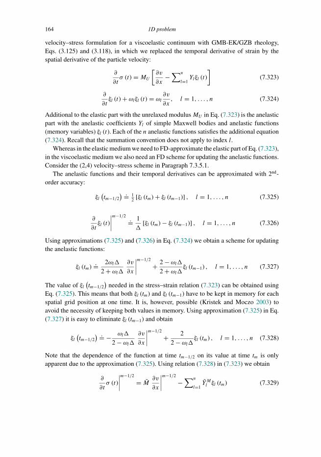
Trim: 247mm × 174mm Top: 14.762mm Gutter: 23.198mmCUUK2497-07 CUUK2497/Moczo ISBN: 978 1 107 02881 4 November 15, 2013 13:36
164 1D problem
velocity–stress formulation for a viscoelastic continuum with GMB-EK/GZB rheology,Eqs. (3.125) and (3.118), in which we replaced the temporal derivative of strain by thespatial derivative of the particle velocity:
∂
∂tσ (t) = MU
[∂v
∂x−∑n
l=1Ylξl (t)
](7.323)
∂
∂tξl (t) + ωlξl (t) = ωl ∂v
∂x, l = 1, . . . , n (7.324)
Additional to the elastic part with the unrelaxed modulusMU in Eq. (7.323) is the anelasticpart with the anelastic coefficients Yl of simple Maxwell bodies and anelastic functions(memory variables) ξl (t). Each of the n anelastic functions satisfies the additional equation(7.324). Recall that the summation convention does not apply to index l.
Whereas in the elastic medium we need to FD-approximate the elastic part of Eq. (7.323),in the viscoelastic medium we also need an FD scheme for updating the anelastic functions.Consider the (2,4) velocity–stress scheme in Paragraph 7.3.5.1.
The anelastic functions and their temporal derivatives can be approximated with 2nd-order accuracy:
ξl(tm−1/2
) .= 12 [ξl (tm) + ξl (tm−1)] , l = 1, . . . , n (7.325)
∂
∂tξl (t)
∣∣∣∣m−1/2.= 1
�[ξl (tm) − ξl (tm−1)] , l = 1, . . . , n (7.326)
Using approximations (7.325) and (7.326) in Eq. (7.324) we obtain a scheme for updatingthe anelastic functions:
ξl (tm).= 2ωl�
2 + ωl�∂v
∂x
∣∣∣∣m−1/2
+ 2 − ωl�2 + ωl�ξl (tm−1) , l = 1, . . . , n (7.327)
The value of ξl(tm−1/2
)needed in the stress–strain relation (7.323) can be obtained using
Eq. (7.325). This means that both ξl (tm) and ξl (tm−1) have to be kept in memory for eachspatial grid position at one time. It is, however, possible (Kristek and Moczo 2003) toavoid the necessity of keeping both values in memory. Using approximation (7.325) in Eq.(7.327) it is easy to eliminate ξl (tm−1) and obtain
ξl(tm−1/2
) .= − ωl�
2 − ωl�∂v
∂x
∣∣∣∣m−1/2
+ 2
2 − ωl�ξl (tm) , l = 1, . . . , n (7.328)
Note that the dependence of the function at time tm−1/2 on its value at time tm is onlyapparent due to the approximation (7.325). Using relation (7.328) in (7.323) we obtain
∂
∂tσ (t)
∣∣∣∣m−1/2
= M ∂v
∂x
∣∣∣∣m−1/2
−∑n
l=1Y Ml ξl (tm) (7.329)
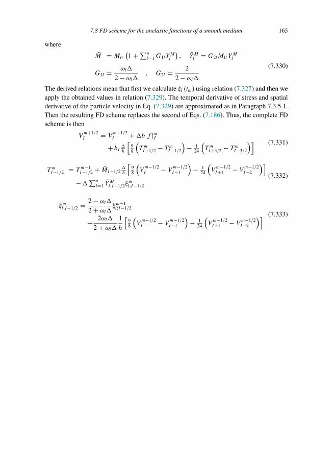
Trim: 247mm × 174mm Top: 14.762mm Gutter: 23.198mmCUUK2497-07 CUUK2497/Moczo ISBN: 978 1 107 02881 4 November 15, 2013 13:36
7.8 FD scheme for the anelastic functions of a smooth medium 165
where
M = MU(1 +∑n
l=1G1lYMl
), YMl = G2lMUY
Ml
G1l = ωl�
2 − ωl� , G2l = 2
2 − ωl�(7.330)
The derived relations mean that first we calculate ξl (tm) using relation (7.327) and then weapply the obtained values in relation (7.329). The temporal derivative of stress and spatialderivative of the particle velocity in Eq. (7.329) are approximated as in Paragraph 7.3.5.1.Then the resulting FD scheme replaces the second of Eqs. (7.186). Thus, the complete FDscheme is then
Vm+1/2I = V m−1/2
I +�b f |mI+ bI �h
[98
(T mI+1/2 − T mI−1/2
)− 1
24
(T mI+3/2 − T mI−3/2
)] (7.331)
T mI−1/2 = T m−1I−1/2 + MI−1/2
�h
[98
(Vm−1/2I − V m−1/2
I−1
)− 1
24
(Vm−1/2I+1 − V m−1/2
I−2
)]−�∑n
l=1 YMl;I−1/2ξ
ml;I−1/2
(7.332)
ξml;I−1/2 = 2 − ωl�2 + ωl�ξ
m−1l;I−1/2
+ 2ωl�
2 + ωl�1
h
[98
(Vm−1/2I − V m−1/2
I−1
)− 1
24
(Vm−1/2I+1 − V m−1/2
I−2
)] (7.333)
Trim: 247mm × 174mm Top: 14.762mm Gutter: 23.198mmCUUK2497-08 CUUK2497/Moczo ISBN: 978 1 107 02881 4 November 16, 2013 8:50
8
3D finite-difference schemes
Before we address particular aspects of the FD schemes, we briefly review the developmentof the application and elaboration of the FDM in numerical modelling of seismic wavepropagation and earthquake motion. We also refer to recent reviews of FD modelling, e.g.,Moczo et al. (2007a,b), Fichtner (2011), Robertsson and Blanch (2011) and Robertssonet al. (2012). The reviews by Robertsson and his colleagues focus on exploration seismologybut they are also relevant for the earthquake seismology. Although related to computationalelectrodynamics, the extensive book by Taflove and Hagness (2005) is also a relevantreference.
8.1 Formulations and grids
8.1.1 Displacement conventional-grid schemes
The pioneering studies of applications of the FDM to seismic wave propagation werebased on a strong displacement formulation and conventional grids. Representative studiesinclude articles by Alterman and Karal (1968), Alterman and Rotenberg (1969), Altermanand Loewenthal (1970), Boore (1970, 1972a,b), Boore et al. (1971), Alford et al. (1974),Ilan et al. (1975), Kelly et al. (1976) and Marfurt (1984). Efforts to improve the displacementconventional-grid schemes (in brief, conventional schemes) continued until about the end of1990s; examples include schemes by Kummer et al. (1987), Zahradnık (1995b), Zahradnıkand Priolo (1995) and Moczo et al. (1999). The last three schemes reached reasonablelevels of accuracy in modelling the planar free surface and material interfaces, but theycould not overcome the fundamental limitations of the conventional schemes.
Bamberger et al. (1980) analyzed grid dispersion and found that the ratio of the gridS-wave phase velocity to the true S-wave velocity becomes infinite inside liquids for theconventional schemes. Stephen (1983), based on numerical tests, pointed out instabilities ofthe heterogeneous conventional FD schemes at a liquid/solid interface. Marfurt (1984) ana-lyzed grid dispersion and concluded that in a homogeneous elastic medium the explicit FEand FD schemes are comparable for Poisson’s ratio less than 0.3; the FE scheme is superiorto the FD for Poisson’s ratio between 0.3 and 0.45; and none of the schemes is economi-cally attractive for Poisson’s ratio greater than 0.45. Moczo et al. (1999) demonstrated thedecreasing accuracy of synthetics with increasing P-wave to S-wave speed ratio (VP /VS).
166

Trim: 247mm × 174mm Top: 14.762mm Gutter: 23.198mmCUUK2497-08 CUUK2497/Moczo ISBN: 978 1 107 02881 4 November 16, 2013 8:50
8.1 Formulations and grids 167
Moczo et al. (2010, 2011) explained why the conventional schemes have a problem withlarge VP /VS (see Section 8.3). Let us finish this very brief overview of the traditional (his-torical) displacement conventional-grid schemes with two important pioneering articles byFrankel and Vidale (1992) and Frankel (1993), which started the important period of 3DFD modelling of earthquake ground motion.
Being motivated by fundamental problems of the traditional (or historical) displace-ment conventional-grid schemes as well as by the difficulty with which the staggered-gridschemes handle complex geometries (e.g., free-surface topography), Kreiss, Petersson,Sjogreen and their collaborators have been developing a systematic novel approach for solv-ing the 2nd-order displacement-formulation equation of motion by the FDM. For example,Nilsson et al. (2007) developed a (2,2) 3D displacement conventional-grid scheme basedon discretization satisfying a summation-by-parts principle. The summation-by-parts dis-cretization guarantees stability of the scheme for allVP /VS values. Nilsson et al. proved thatthe discrete energy is conserved by the scheme, for equations with variable coefficients ona bounded domain with traction-free or Dirichlet boundary conditions. Appelo and Peters-son (2009) generalized the summation-by-parts approach to curvilinear grids, allowing thefree surface boundary condition to be imposed along a realistic topography. More recently,Sjogreen and Petersson (2012) generalized the approach by Nilsson et al. (2007) and devel-oped a 2D (4,4) scheme for solving the 2nd-order displacement-formulation equation ofmotion. Their spatial discretization satisfies the summation-by-parts principle and allowsfor heterogeneous materials and traction-free boundary conditions. The essential elementin their generalization is the 4th-order accurate approximation of the 2nd spatial derivativewith a variable coefficient, e.g., ∂
∂x
(μ(x) ∂u
∂x
), consistent with the approximation of the 2nd
mixed spatial derivative, e.g., ∂∂x
(μ(x) ∂u
∂y
), such that an energy estimate can be obtained.
Compared to the previous summation-by-parts approximations, they use one virtual pointoutside the physical boundary. This makes it possible to enforce boundary conditions in apoint-wise manner and avoid the use of projections or penalty terms. The explicit 4th-orderaccurate temporal discretization is energy conserving.
Kreiss and Petersson (2012) analyzed the (homogeneous medium) half-plane problemof the 2nd-order displacement-formulation equation of motion subject to the traction-freeboundary condition. They developed a normal mode analysis using a modified equationapproach and analyzed the influence of truncation errors in a pth-order accurate numericalapproximation of the free surface boundary condition. They explained why the num-ber of grid points per wavelength of the surface Rayleigh wave must be proportional to(VP /VS)2/p to achieve a constant phase error in the numerical solution when VP /VS is verylarge.
8.1.2 Velocity–stress staggered-grid schemes
Problems with instabilities and numerical dispersion produced by the mixed boundary con-ditions in the conventional schemes led Madariaga (1974, 1976) to introduce the velocity–stress staggered-grid (VS SG) scheme motivated by the staggered-grid scheme developed

Trim: 247mm × 174mm Top: 14.762mm Gutter: 23.198mmCUUK2497-08 CUUK2497/Moczo ISBN: 978 1 107 02881 4 November 16, 2013 8:50
168 3D finite-difference schemes
by Yee (1966) for solving Maxwell’s equations. Madariaga used the formulation for mod-elling rupture propagation. Virieux and Madariaga (1982) further elaborated the VS SGscheme for studying dynamic shear cracks. Virieux (1984) introduced the 2D (2,2) VS SGscheme for modelling SH waves and Virieux (1986) presented the corresponding P-SVscheme. Virieux (1986) found that the stability condition of his P-SV scheme as well as thegrid P-wave phase velocity is independent of Poisson’s ratio. The grid S-wave phase veloc-ity depends on Poisson’s ratio (through VP /VS) but is rather insensitive to VP /VS , and itsbehaviour does not degrade with increasing VP /VS . None of these properties is the case forthe conventional schemes. The staggered-grid schemes have become the dominant type ofschemes in the FD modelling of seismic wave propagation and earthquake motion. In orderto decrease the number of grid points per minimum wavelength and thus increase compu-tational efficiency, Levander (1988) introduced the 4th-order approximation in space in his2D P-SV (2,4) VS SG scheme. Graves (1993), Olsen (1994) and Pitarka et al. (1997) intro-duced 3D (2,4) VS SG schemes, applied them to modelling of earthquake ground motion,and significantly promoted the FD modelling of earthquake ground motion. Yomogida andEtgen (1993) developed the (2,8) displacement–stress staggered-grid scheme and appliedit for modelling wave propagation in the Los Angeles basin for the 1988 Whittier Narrowsearthquake.
Igel et al. (1995) described the problems of the staggered-grid schemes in modellingseismic wave propagation in anisotropic media. Recently, Lisitsa and Vishnevskiy (2010)and Bernth and Chapman (2011) showed the generalization of the standard staggered gridto the so-called Lebedev grid, which may be considered a natural choice for an anisotropicmedium.
8.1.3 Displacement–stress schemes on the grid staggered in space
In order to further reduce the memory requirements, Luo and Schuster (1990) suggested adisplacement–stress 2D P-SV scheme which they called a parsimonious scheme. Becausethe scheme does not integrate stress in time, the stress-tensor components are only temporaryquantities and the scheme is staggered only in space. The displacement–stress scheme in 3Dneeds only 75% of the memory needed by the velocity–stress scheme. Rodrigues (1993)and Yomogida and Etgen (1993) developed (2,8) 3D displacement–stress schemes, andMoczo et al. (2002) a (2,4) scheme with volume harmonic averaging of elastic moduli andvolume arithmetic averaging of density.
8.1.4 Velocity–stress partly-staggered-grid schemes
For imposing the fault boundary conditions in modelling rupture dynamics, Andrews(1973) and independently Day (1977, 1982) introduced the partly staggered grid. Magnieret al. (1994) elaborated the partly-staggered-grid scheme in order to incorporate anisotropy –a task not natural for staggered-grid schemes. Zhang (1997, 1999) presented his
Trim: 247mm × 174mm Top: 14.762mm Gutter: 23.198mmCUUK2497-08 CUUK2497/Moczo ISBN: 978 1 107 02881 4 November 16, 2013 8:50
8.1 Formulations and grids 169
quadrangle-grid velocity–stress scheme which is, in fact, the partly-staggered-grid scheme.Saenger and his colleagues (e.g., Saenger et al, 2000, Saenger and Bohlen 2004, Bohlen andSaenger 2006) elaborated and considerably promoted the application of partly-staggered-grid schemes. Saenger and his colleagues use the term ‘new rotated staggered grid’. In fact,the grid in their articles was not new and the term ‘rotated’ reflects one feature of one partic-ular partly-staggered-grid scheme, which is not substantial. The (2,2) displacement–stressversion of the partly-staggered-grid scheme is equivalent to the standard (2,2) FE scheme(see Section 8.2). Consequently and inherently, it may have a problem with the hourglassmodes that have to be artificially suppressed.
8.1.5 Optimally accurate schemes
In the era of the staggered-grid schemes, Geller and Takeuchi (1995, 1998) and Takeuchi andGeller (2000) made an important contribution to the theory of the FD schemes and developedtheir optimally accurate FD schemes in application to the Galerkin-type weak form ofStrang and Fix (1973) and Geller and Ohminato (1994). In their schemes displacement isthe sole dependent variable, in contrast to the staggered-grid schemes. The clever idea ofGeller and Takeuchi (1995) was to minimize the error of the numerical solution first of allat eigenfrequencies (or resonant frequencies), that is, at frequencies at which oscillatorymotion of a linear mechanical system or finite volume of elastic continuum is naturally mostamplified. Geller and Takeuchi (1995) used the 1st-order Born theory and a normal modeexpansion to obtain formal estimates of the relative error of the numerical solution and ageneral criterion for what they named optimally accurate operators. The criterion requiresthat the inner product of an eigenfunction and the net error of the discretized equation ofmotion should be approximately equal to zero when the operand is the eigenfunction and thefrequency is equal to the corresponding eigenfrequency. The criterion can be used to deriveoptimally accurate operators without knowing the actual values of the eigenfrequenciesand eigenfunctions. Geller and Takeuchi (1995) showed that in the case of a heterogeneousmedium the criterion is the logical extension of the criterion to minimize grid dispersion ofphase velocity for a homogeneous medium. Geller and Takeuchi (1998) used the criterionto develop an optimally accurate 2nd-order FDTD scheme for the elastic 1D case. Takeuchiand Geller (2000) then developed optimally accurate FDTD operators for the 2D and 3Dcases. Mizutani (2002) developed a scheme capable of accounting for an arbitrary positionof the material discontinuity in the grid.
Whereas optimally accurate FDTD schemes require at least twice the CPU time per gridpoint and time step compared to 2nd-order staggered-grid FD schemes, they yield accuracyimprovements on the order of 10 (for 1D), 50 (for 2D), or 100 (for 3D). From this point ofview they are cost effective.
The optimization yields implicit schemes. Geller and Takeuchi (1998) applied thepredictor-corrector algorithm in order to avoid solving large systems of algebraic equa-tions. Thus, the actual computational schemes are explicit.
Trim: 247mm × 174mm Top: 14.762mm Gutter: 23.198mmCUUK2497-08 CUUK2497/Moczo ISBN: 978 1 107 02881 4 November 16, 2013 8:50
170 3D finite-difference schemes
Kristek and Moczo (2006) numerically compared the 1D (2,2) conventional scheme, the(2,4) staggered-grid scheme and the optimally accurate scheme. The results confirmed thesuperior accuracy of the optimally accurate scheme with almost negligible grid dispersion.
Despite its superior accuracy, we do not apply the optimally accurate scheme for mod-elling earthquake motion in surface local structures. This is because the conventionalscheme serves as a predictor. Consequently, the predictor is in media with large VP /VS soinaccurate that the corrector is not capable to ‘correct’ the ‘predicted’ values.
In media with low VP /VS the scheme is probably the most accurate FD scheme.
8.1.6 Velocity–stress schemes on the collocated grid
The ‘ultimate’ grid for the velocity–stress schemes should be the collocated grid (alsononstaggered or unstaggered) in which all particle-velocity and stress-tensor componentsshare each grid position. From this point of view, the collocated grid is a natural grid notonly for imposing boundary conditions (at the planar or nonplanar free surface, materialinterface or dynamically rupturing fault) but also for anisotropic media. It is, however,necessary to avoid the centred approximations of temporal and spatial derivatives. Theiruse would cause the presence of odd–even decoupling in time and space. Zhang and Chen(2006) and Zhang et al. (2012) therefore applied a MacCormack scheme in which thecentred approximation is split into forward and backward approximations. The original(2,2) MacCormack scheme (MacCormack 1969) was extended to the (2,4) scheme byGottlieb and Turkel (1976). Bayliss et al. (1986) combined the scheme with the operatorsplitting-time integration. Zhang and Chen (2006) and Zhang et al. (2012) developed a(4,4) MacCormack-type scheme in which one-sided operators are alternately applied in themultistage Runge–Kutta time integration algorithm. The applied one-sided approximationswere developed by Tam and Webb (1993) and Hixon (1997).
Here we do not review the development of other aspects of FD schemes. The devel-opments are concisely characterized in the chapters on rheological models, free surfaces,discontinuous grids, PML, earthquake source dynamics and in the following sections ofthis chapter.
8.2 Schemes on staggered, partly staggered, collocated and conventional grids
In this section we assume a smoothly and weakly heterogeneous isotropic elastic unboundedmedium. We briefly indicate the velocity–stress staggered-grid and partly-staggered-gridschemes as well as the displacement conventional-grid scheme. For brevity, recall just theequations for vx and σxx :
ρ∂vx
∂t= ∂σxx
∂x+ ∂σxy∂y
+ ∂σxz∂z
+ fx∂σxx
∂t= (λ+ 2μ)
∂vx
∂x+ μ∂vy
∂y+ μ∂vz
∂z
(8.1)

Trim: 247mm × 174mm Top: 14.762mm Gutter: 23.198mmCUUK2497-08 CUUK2497/Moczo ISBN: 978 1 107 02881 4 November 16, 2013 8:50
8.2 Schemes on grids 171
/2h
1/2mVX +
1/2mVY +
1/2mVZ +
, ,m m mTXX TYY TZZ
mTXY
mTYZ
mTZX
Figure 8.1 Grid cell of the staggered grid.
in the velocity–stress formulation and
ρ∂2ux
∂t2= ∂
∂x
[(λ+ 2μ)
∂ux
∂x
]+ ∂
∂y
(μ∂ux
∂y
)+ ∂
∂z
(μ∂ux
∂z
)
+ ∂
∂x
(λ∂uy
∂y
)+ ∂
∂x
(λ∂uz
∂z
)+ ∂
∂y
(μ∂uy
∂x
)+ ∂
∂z
(λ∂uz
∂x
)+ fx
(8.2)
in the displacement formulation. Denote the discrete grid values of the particle-velocitycomponents vx, vy, vz by VX, VY, VZ, respectively. Similarly denote the stress-tensor com-ponents σxx, σxy, σzx by TXX,TXY,TZX.
8.2.1 (2,4) velocity stress scheme on the staggered grid
Figure 8.1 shows the grid cell. We may approximate the first of Eqs. (8.1) at the timelevel m and spatial grid position I,K + 1/2, L+ 1/2. In the staggered grid we have allquantities exactly at the positions at which we need them for the most natural approxi-mations of derivatives. The spatial distribution is unambiguous, complementary and thereis no redundancy. This is the beauty of the staggered grid. The schemes for vx and σxxare
VXm+1/2I,K+1/2,L+1/2
= VXm−1/2I,K+1/2,L+1/2 + �
ρI,K+1/2,L+1/2f |mI,K+1/2,L+1/2
+ 1
ρI,K+1/2,L+1/2
�
h
[98
(TXXmI+1/2,K+1/2,L+1/2 − TXXmI−1/2,K+1/2,L+1/2
)− 1
24
(TXXmI+3/2,K+1/2,L+1/2 − TXXmI−3/2,K+1/2,L+1/2
)+ 9
8
(TXYmI,K+1,L+1/2 − TXYmI,K,L+1/2
)− 1
24
(TXYmI,K+2,L+1/2 − TXYmI,K−1,L+1/2
)+ 9
8
(TZXmI,K+1/2,L+1 − TZXmI,K+1/2,L
)− 1
24
(TZXmI,K+1/2,L+2 − TZXmI,K+1/2,L−1
)]
(8.3)

Trim: 247mm × 174mm Top: 14.762mm Gutter: 23.198mmCUUK2497-08 CUUK2497/Moczo ISBN: 978 1 107 02881 4 November 16, 2013 8:50
172 3D finite-difference schemes
1/2 1/2 1/2, ,m m mVX VY VZ+ + +h
, ,
, ,
m m m
m m m
TXX TYY TZZ
TXY TYZ TZX
Figure 8.2 Grid cell of the partly staggered grid.
and
TXXmI+1/2,K+1/2,L+1/2
= TXXm−1I+1/2,K+1/2,L+1/2
+ �h
{(λ+ 2μ)I+1/2,K+1/2,L+1/2
[98
(VX
m−1/2I+1,K+1/2,L+1/2 − VXm−1/2
I,K+1/2,L+1/2
)− 1
24
(VX
m−1/2I+2,K+1/2,L+1/2 − VXm−1/2
I−1,K+1/2,L+1/2
)]+ λI+1/2,K+1/2,L+1/2
[98
(V Y
m−1/2I+1/2,K+1,L+1/2 − V Ym−1/2
I+1/2,K,L+1/2
)− 1
24
(V Y
m−1/2I+1/2,K+2,L+1/2 − V Ym−1/2
I+1/2,K−1,L+1/2
)]+ λI+1/2,K+1/2,L+1/2
[98
(VZ
m−1/2I+1/2,K+1/2,L+1 − VZm−1/2
I+1/2,K+1/2,L
)− 1
24
(VZ
m−1/2I+1/2,K+1/2,L+2 − VZm−1/2
I+1/2,K+1/2,L−1
)]}
(8.4)
On the other hand, we can immediately realize that it would be useful to have all particle-velocity components at the same grid position because this is what we have from measure-ments. It would be also useful to have all stress-tensor components at the same grid positionbecause this would ease the simulation of the traction-free condition at the free surface.Finally, it would be useful to have all field variables at the same position for imposingboundary conditions at internal interfaces and, of course, for modelling wave propagationin anisotropic media. The mentioned aspects are partly addressed by schemes on the partlystaggered grid.
8.2.2 (2,4) velocity–stress scheme on the partly staggered grid
Figure 8.2 shows the grid cell. Consider first approximating the spatial derivative of σxx :
∂σxx
∂x
∣∣∣∣mI
≈ 98
(TXXmI+1/2 − TXXmI−1/2
)− 124
(TXXmI+3/2 − TXXmI−3/2
)(8.5)

Trim: 247mm × 174mm Top: 14.762mm Gutter: 23.198mmCUUK2497-08 CUUK2497/Moczo ISBN: 978 1 107 02881 4 November 16, 2013 8:50
8.2 Schemes on grids 173
Because we do not have the TXX values along the grid line parallel with the x-axis andgoing through the grid positions with indices (K, L), we approximate the derivative as anarithmetic average of approximations (8.5) along four grid lines parallel with the x-axis andgoing through the grid positions with indices (K − 1/2, L− 1/2), (K − 1/2, L+ 1/2),(K + 1/2, L− 1/2) and (K + 1/2, L+ 1/2), respectively. Similarly, we approximate allspatial derivatives. The resulting schemes are
VXm+1/2I,K,L = VXm−1/2
I,K,L + �
ρI,K,Lf |mI,K,L + 1
ρI,K+1/2,L+1/2
× �4h
{98
(TXXmI+1/2,K−1/2,L−1/2 − TXXmI−1/2,K−1/2,L−1/2
)− 1
24
(TXXmI+3/2,K−1/2,L−1/2 − TXXmI−3/2,K−1/2,L−1/2
)+ 9
8
(TXXmI+1/2,K−1/2,L+1/2 − TXXmI−1/2,K−1/2,L+1/2
)− 1
24
(TXXmI+3/2,K−1/2,L+1/2 − TXXmI−3/2,K−1/2,L+1/2
)+ 9
8
(TXXmI+1/2,K+1/2,L−1/2 − TXXmI−1/2,K+1/2,L−1/2
)− 1
24
(TXXmI+3/2,K+1/2,L−1/2 − TXXmI−3/2,K+1/2,L−1/2
)+ 9
8
(TXXmI+1/2,K+1/2,L+1/2 − TXXmI−1/2,K+1/2,L+1/2
)− 1
24
(TXXmI+3/2,K+1/2,L+1/2 − TXXmI−3/2,K+1/2,L+1/2
)+ 9
8
(TXYmI−1/2,K+1/2,L−1/2 − TXYmI−1/2,K−1/2,L−1/2
)− 1
24
(TXYmI−1/2,K+3/2,L−1/2 − TXYmI−1/2,K−3/2,L−1/2
)+ 9
8
(TXYmI−1/2,K+1/2,L+1/2 − TXYmI−1/2,K−1/2,L+1/2
)− 1
24
(TXYmI−1/2,K+3/2,L+1/2 − TXYmI−1/2,K−3/2,L+1/2
)+ 9
8
(TXYmI+1/2,K+1/2,L−1/2 − TXYmI+1/2,K−1/2,L−1/2
)− 1
24
(TXYmI+1/2,K+3/2,L−1/2 − TXYmI+1/2,K−3/2,L−1/2
)+ 9
8
(TXYmI+1/2,K+1/2,L+1/2 − TXYmI+1/2,K−1/2,L+1/2
)− 1
24
(TXYmI+1/2,K+3/2,L+1/2 − TXYmI+1/2,K−3/2,L+1/2
)+ 9
8
(TXZmI−1/2,K−1/2,L+1/2 − TXZmI−1/2,K−1/2,L−1/2
)− 1
24
(TXZmI−1/2,K−1/2,L+3/2 − TXZmI−1/2,K−1/2,L−3/2
)
(8.6)
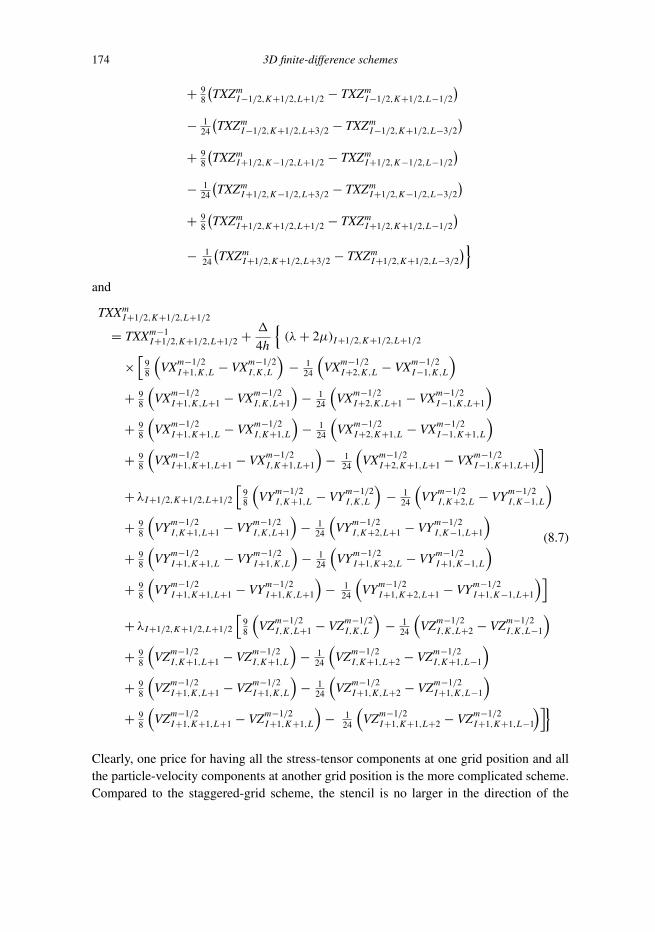
Trim: 247mm × 174mm Top: 14.762mm Gutter: 23.198mmCUUK2497-08 CUUK2497/Moczo ISBN: 978 1 107 02881 4 November 16, 2013 8:50
174 3D finite-difference schemes
+ 98
(TXZmI−1/2,K+1/2,L+1/2 − TXZmI−1/2,K+1/2,L−1/2
)− 1
24
(TXZmI−1/2,K+1/2,L+3/2 − TXZmI−1/2,K+1/2,L−3/2
)+ 9
8
(TXZmI+1/2,K−1/2,L+1/2 − TXZmI+1/2,K−1/2,L−1/2
)− 1
24
(TXZmI+1/2,K−1/2,L+3/2 − TXZmI+1/2,K−1/2,L−3/2
)+ 9
8
(TXZmI+1/2,K+1/2,L+1/2 − TXZmI+1/2,K+1/2,L−1/2
)− 1
24
(TXZmI+1/2,K+1/2,L+3/2 − TXZmI+1/2,K+1/2,L−3/2
)}and
TXXmI+1/2,K+1/2,L+1/2
= TXXm−1I+1/2,K+1/2,L+1/2 + �
4h
{(λ+ 2μ)I+1/2,K+1/2,L+1/2
×[
98
(VXm−1/2
I+1,K,L − VXm−1/2I,K,L
)− 1
24
(VXm−1/2
I+2,K,L − VXm−1/2I−1,K,L
)+ 9
8
(VXm−1/2
I+1,K,L+1 − VXm−1/2I,K,L+1
)− 1
24
(VXm−1/2
I+2,K,L+1 − VXm−1/2I−1,K,L+1
)+ 9
8
(VXm−1/2
I+1,K+1,L − VXm−1/2I,K+1,L
)− 1
24
(VXm−1/2
I+2,K+1,L − VXm−1/2I−1,K+1,L
)+ 9
8
(VXm−1/2
I+1,K+1,L+1 − VXm−1/2I,K+1,L+1
)− 1
24
(VXm−1/2
I+2,K+1,L+1 − VXm−1/2I−1,K+1,L+1
)]+ λI+1/2,K+1/2,L+1/2
[98
(VYm−1/2
I,K+1,L − VYm−1/2I,K,L
)− 1
24
(VYm−1/2
I,K+2,L − VYm−1/2I,K−1,L
)+ 9
8
(VYm−1/2
I,K+1,L+1 − VYm−1/2I,K,L+1
)− 1
24
(VYm−1/2
I,K+2,L+1 − VYm−1/2I,K−1,L+1
)+ 9
8
(VYm−1/2
I+1,K+1,L − VYm−1/2I+1,K,L
)− 1
24
(VYm−1/2
I+1,K+2,L − VYm−1/2I+1,K−1,L
)+ 9
8
(VYm−1/2
I+1,K+1,L+1 − VYm−1/2I+1,K,L+1
)− 1
24
(VYm−1/2
I+1,K+2,L+1 − VYm−1/2I+1,K−1,L+1
)]+ λI+1/2,K+1/2,L+1/2
[98
(VZm−1/2
I,K,L+1 − VZm−1/2I,K,L
)− 1
24
(VZm−1/2
I,K,L+2 − VZm−1/2I,K,L−1
)+ 9
8
(VZm−1/2
I,K+1,L+1 − VZm−1/2I,K+1,L
)− 1
24
(VZm−1/2
I,K+1,L+2 − VZm−1/2I,K+1,L−1
)+ 9
8
(VZm−1/2
I+1,K,L+1 − VZm−1/2I+1,K,L
)− 1
24
(VZm−1/2
I+1,K,L+2 − VZm−1/2I+1,K,L−1
)+ 9
8
(VZm−1/2
I+1,K+1,L+1 − VZm−1/2I+1,K+1,L
)− 1
24
(VZm−1/2
I+1,K+1,L+2 − VZm−1/2I+1,K+1,L−1
)]}
(8.7)
Clearly, one price for having all the stress-tensor components at one grid position and allthe particle-velocity components at another grid position is the more complicated scheme.Compared to the staggered-grid scheme, the stencil is no larger in the direction of the
Trim: 247mm × 174mm Top: 14.762mm Gutter: 23.198mmCUUK2497-08 CUUK2497/Moczo ISBN: 978 1 107 02881 4 November 16, 2013 8:50
8.2 Schemes on grids 175
spatial derivative but it is wider in the directions perpendicular to the direction of the spatialderivative. The other price is not obvious. It is the principal possibility of hourglass (orzero-energy) modes. These have to be suppressed, for example, by introducing artificialattenuation.
The presence of hourglass modes can be easily understood based on the equivalence ofthe (2,2) displacement–stress partly staggered scheme with the standard (2,2) displacementFE scheme with Gaussian 1-point integration – see Moczo et al. (2010, 2011).
Recall that the partly-staggered-grid schemes are also called rotated staggered-gridschemes according to articles by Sanger and his colleagues. We prefer the term ‘partly-staggered-grid schemes’ because the aspect of rotation in one particular scheme is notthe most substantial aspect and this type of scheme was developed earlier without anyrotation.
8.2.3 (4,4) velocity–stress scheme on the collocated grid
In the velocity–stress formulation in matrix form a vector of field variables is defined thatcomprises all particle-velocity and stress-tensor components. The use of the collocatedgrid makes it possible to have all nine field variables at each grid position. Applicationof centred FD approximations leads to odd–even decoupling. The standard 2nd-order andalso 4th-order approximations (based on Taylor expansions) have large truncation errorscompared to the approximations on the staggered grid. Zhang and Chen (2006) and Zhanget al. (2012) overcome these problems using a higher-order MacCormack scheme that usesa combination of the (noncentred) one-sided approximations in the multistage Runge–Kuttatime-integration algorithm. The one-sided approximations are based on minimization ofthe dispersion error. As we indicated in Chapter 7, the effective resulting stencil is relativelylong. Because the presentation of the 3D scheme is rather lengthy we refer to the article byZhang et al. (2012).
8.2.4 Displacement scheme on the conventional grid
In Subsection 7.3.1 we showed how to avoid the spatial differentiation of the elastic modulusby using a mathematical trick suggested by Tikhonov and Samarskii. We could apply thesame trick also in 3D. Moczo et al. (1999) presented the 3D (2,2) displacement conventionalgrid scheme as a generalization of the 2D scheme suggested by Zahradnık (1995b) andZahradnık and Priolo (1995); see also Moczo et al. (2007a). While reasonably accurate ina heterogeneous medium the scheme has fundamental drawbacks: (1) its accuracy rapidlydecreases with increasing value of the P-wave to S-wave speed ratio; (2) it is unstableat the solid–liquid interface; (3) it is computationally inefficient due to the (2,2) orderof approximation. As far as we know, a displacement scheme on the conventional gridthat would overcome all three problems has not been found. In the following section wepresent two (2,4) displacement conventional-grid schemes, but only for the homogeneousmedium.

Trim: 247mm × 174mm Top: 14.762mm Gutter: 23.198mmCUUK2497-08 CUUK2497/Moczo ISBN: 978 1 107 02881 4 November 16, 2013 8:50
176 3D finite-difference schemes
Here, we merely point out the aspect that appears to be the key problem even in ahomogeneous medium. Consider, for example, the most straightforward 2nd-order approxi-mations:
μ∂2ux
∂y2
∣∣∣∣mI,K,L
= μ1
h
[1
h
(UXmI,K+1,L − UXmI,K,L
)− 1
h
(UXmI,K,L − UXmI,K−1,L
)]
μ∂2uy
∂y∂x
∣∣∣∣mI,K,L
= μ 1
2h
[1
2h
(UYmI+1,K+1,L − UYmI+1,K−1,L
)− 1
2h
(UYmI−1,K+1,L − UYmI−1,K−1,L
)](8.8)
In the case of the 2nd nonmixed derivative we first approximate the 1st derivatives atI,K + 1/2, L and I,K − 1/2, L, each over the grid spacing h, and then we approximatethe derivative of the 1st derivative at I, K, L, again over h. In the case of the 2nd mixedderivative we first approximate the x-derivative at I, K, L over 2h and then we approximatethe y-derivative of the x-derivative at I, K, L, again over 2h. Moczo et al. (2010, 2011) showedthat the inhomogeneity in approximating derivatives – once over h, the other time over 2h –is the reason for the degrading accuracy of the standard-displacement conventional gridwith increasing P-wave to S-wave speed ratio. Note that in the velocity–stress (or possiblydisplacement–stress) schemes on the staggered, partly staggered and collocated grids thereis no inhomogeneity in approximating spatial derivatives.
In Section 8.1 we mentioned a novel approach based on the summation-by-parts principle(e.g., Nilsson et al. 2007, Kreiss and Petersson 2012, Sjogreen and Petersson 2012). Forthe recent (4,4) scheme we refer to the article by Sjogreen and Petersson (2012).
8.3 Accuracy of FD schemes with respect to P-wave to S-wave ratio:analysis of local errors
A P-wave to S-wave speed ratio in surface sediments as large as 5 or more often has tobe accounted for in the numerical modelling of seismic motion in sedimentary basins andvalleys. Five is a common value in surface sediments, mainly under the water level, and 10,though relatively large, certainly is not the maximum possible value in the unconsolidatedsurface water-saturated sediments.
8.3.1 Equations and FD schemes
8.3.1.1 Equations
Consider an unbounded homogeneous perfectly elastic isotropic medium. The P-wave andS-wave speeds are VP ≡ α ≡ [(λ+ 2μ)/ρ]1/2 and VS ≡ β ≡ (μ/ρ)1/2, respectively. Here

Trim: 247mm × 174mm Top: 14.762mm Gutter: 23.198mmCUUK2497-08 CUUK2497/Moczo ISBN: 978 1 107 02881 4 November 16, 2013 8:50
8.3 Accuracy with respect to P-wave to S-wave ratio 177
ρ is density, λ and μ are Lame elastic moduli. Define the P-wave to S-wave speed ratioVP /VS or r:
r ≡ α/β (8.9)
Throughout the chapter, r and VP /VS , α and VP , and β and VS will be used interchangeablyfor convenience. Consider the displacement–stress (DS) formulation of the equation ofmotion, (2.28) and (2.23), and the displacement (D) formulation, (2.29). The latter may bewritten as
∂2ux
∂t2= α2
(∂2ux
∂x2+ ∂2uy
∂y∂x+ ∂2uz
∂z∂x
)+ β2
(∂2ux
∂y2− ∂2uy
∂y∂x+ ∂
2ux
∂z2− ∂2uz
∂z∂x
)∂2uy
∂t2= α2
(∂2uy
∂y2+ ∂2uz
∂z∂y+ ∂2ux
∂x∂y
)+ β2
(∂2uy
∂z2− ∂2uz
∂z∂y+ ∂
2uy
∂x2− ∂2ux
∂x∂y
)∂2uz
∂t2= α2
(∂2uz
∂z2+ ∂2ux
∂x∂z+ ∂2uy
∂y∂z
)+ β2
(∂2uz
∂x2− ∂2ux
∂x∂z+ ∂
2uz
∂y2− ∂2uy
∂y∂z
) (8.10)
8.3.1.2 FD schemes
The FD schemes differ from each other by the equation formulation, grid and order ofapproximation. For conciseness we will use acronyms for the analyzed schemes: D indicatesthe displacement formulation, DS the displacement–stress formulation; CG indicates theconventional grid, PSG the partly staggered grid, and SG the (spatially) staggered grid.The first number in parentheses indicates the order of approximation in time, the secondnumber the order of approximation in space. The lower-case ‘a’ or ‘b’ indicates one of twovariants of the 4th-order approximation. The schemes included in the analysis are:
FD D CG (2,2) traditional FD displacement conventional grid, 2nd order in time, 2nd
order in spaceFD DS PSG (2,2) FD displacement–stress partly staggered grid, 2nd order in time, 2nd
order in spaceFD DS SG (2,2) FD displacement–stress (spatially) staggered grid, 2nd order in time,
2nd order in spaceFD D CG (2,4a) FD displacement conventional grid, 2nd order in time, 4th order in
space, variant aFD D CG (2,4b) FD displacement conventional grid, 2nd order in time, 4th order in
space, variant bFD DS SG (2,4) FD displacement–stress (spatially) staggered grid 2nd order in time,
4th order in space
FD D CG (2,2), FD D CG (2,4a), FD D CG (2,4b) FD D CG (2,2), the 2nd-order FDscheme solving the strong-form equation of motion for displacement on the conventionalgrid, is obtained if the derivatives in Eqs. (8.10) are replaced using standard 2nd-ordercentred FD formulas approximating the 2nd nonmixed and mixed derivatives.

Trim: 247mm × 174mm Top: 14.762mm Gutter: 23.198mmCUUK2497-08 CUUK2497/Moczo ISBN: 978 1 107 02881 4 November 16, 2013 8:50
178 3D finite-difference schemes
On the conventional grid we can find several-order approximations to the 2nd non-mixed and mixed spatial derivatives. Here we consider two different schemes. FD D CG(2,4a) is the scheme with the minimum possible equal coefficients of the leading termsof the truncation errors for the mixed and nonmixed derivatives. FD D CG (2,4b) hasthe minimum possible spatial stencil and a relatively large difference between values ofcoefficients of the leading terms of the truncation errors for the mixed and nonmixedderivatives.
FD DS SG (2,2), FD DS SG (2,4) FD DS SG (2,2) is obtained in the following way: The2nd temporal derivative in Eqs. (2.28) is replaced using the standard 2nd-order centred FDformula (approximating the 2nd derivative). The 1st spatial derivatives of the stress-tensorcomponents in Eqs. (2.28) are replaced using the standard 2nd-order centred FD formula(approximating the 1st derivative). Then all the discrete stress-tensor components on ther.h.s. of the obtained schemes are replaced by their FD approximations. The approximationsare obtained from Eqs. (2.23) in which the 1st derivatives are replaced using the standard 2nd-order centred FD formula (approximating the 1st derivative). In the resulting final scheme,only displacement components appear. This is important to note, given the fact that thescheme solves the DS formulation of the equation of motion on the spatially staggered grid.Note that this type of scheme is also called the parsimonious scheme.
FD DS SG (2,4) is obtained in the same way except that 4th-order FD approximationsare used to replace the 1st spatial derivatives of the stress-tensor and displacement compo-nents.
FD DS PSG (2,2) It is reasonable to compare this 2nd-order scheme solving the DSformulation of the equation of motion on the partly staggered grid with FD D CG (2,2)and FD DS SG (2,2). The scheme is obtained in the same way as FD DS SG (2,2) exceptthat the FD approximations are more complicated. The complication is due to the fact thatthe stress-tensor components are displaced from the displacement components by half-gridspacing in all three Cartesian directions (Fig. 6.1). For example, in approximating the x-derivative of the stress-tensor component at a grid position of the displacement component,the required values of the stress-tensor components are obtained as arithmetic averagesof the values at four stress-tensor component grid positions in the corresponding yz-gridplanes.
We do not include the velocity–stress staggered-grid (VS SG) schemes. They differ fromthe FD DS SG schemes only in approximating temporal derivatives. Moczo et al. (2010)showed that the difference between the behaviours of the corresponding 2D schemes withrespect to the VP /VS ratio is negligible.
8.3.1.3 Unified representation of FD schemes
All schemes can be represented in a unified form. Let Umξ = Umξ (I,K,L) be a discreteapproximation to uξ (Ih,Kh,Lh,m�) = uξ (xI , yK, zL, tm) with ξ ∈ {x, y, z}, h being a

Trim: 247mm × 174mm Top: 14.762mm Gutter: 23.198mmCUUK2497-08 CUUK2497/Moczo ISBN: 978 1 107 02881 4 November 16, 2013 8:50
8.3 Accuracy with respect to P-wave to S-wave ratio 179
Table 8.1 Grid positions and weight coefficients for the Dxx operators definedby Eq. (8.12)
�j 576wxxj
Dschemexx j = 0 j = 1 j = 2 j = 3 j = 0 j = 1 j = 2 j = 3
DFD D CG (2,2)xx 0 1 −576 576
DFD DS SG (2,2)xx 0 1 −576 576
DFD D CG (2,4a)xx 0 1 2 3 −400 288 144 −32
DFD D CG (2,4b)xx 0 1 2 −720 768 −48
DFD DS SG (2,4)xx 0 1 2 3 −730 783 −54 1
grid spacing in each of the three Cartesian directions and � a time step. Each numericalscheme can be then written as (compare with Eqs. (8.10))
Um+1x = 2Umx − Um−1
x +�2β2{r2(Dxx
[Umx
]+Dyx[Umy
]+Dzx[Umz
])+Dyy
[Umx
]−Dyx[Umy
]+Dzz[Umx
]−Dzx[Umz
]}Um+1y = 2Umy − Um−1
y +�2β2{r2(Dyy
[Umy
]+Dzy[Umz
]+Dxy[Umx
])+Dzz
[Umy
]−Dzy[Umz
]+Dxx[Umy
]−Dxy[Umx
]}Um+1z = 2Umz − Um−1
z +�2β2{r2(Dzz
[Umz
]+Dxz[Umx
]+Dyz[Umy
])+Dxx
[Umz
]−Dxz[Umx
]+Dyy[Umz
]−Dyz[Umy
]}
(8.11)
The schemes differ from each other by the difference operators Dξξ and Dξη; ξ, η ∈{x, y, z} for approximating 2nd nonmixed and mixed spatial derivatives. For brevity weexplicitly show only Dxx and Dzx operators. The other operators are easily obtained byeven permutation of the Cartesian indices.
In the set of the considered schemes we can recognize two types of nonmixed operators.The first type can be expressed as
Dxx [� (I,K,L)] = 1
h2
J∑j=0
wxxj[�(I −�j,K,L
)+� (I +�j,K,L)]
(8.12)
Here � represents a displacement component. According to Eq. (8.12), operators of dif-ferent schemes may differ from each other by the number of grid positions at whichdisplacement components are used for the approximation and the weight coefficients wxxjof the considered displacement component at those grid positions. The grid positions andweight coefficients are given in Table 8.1.
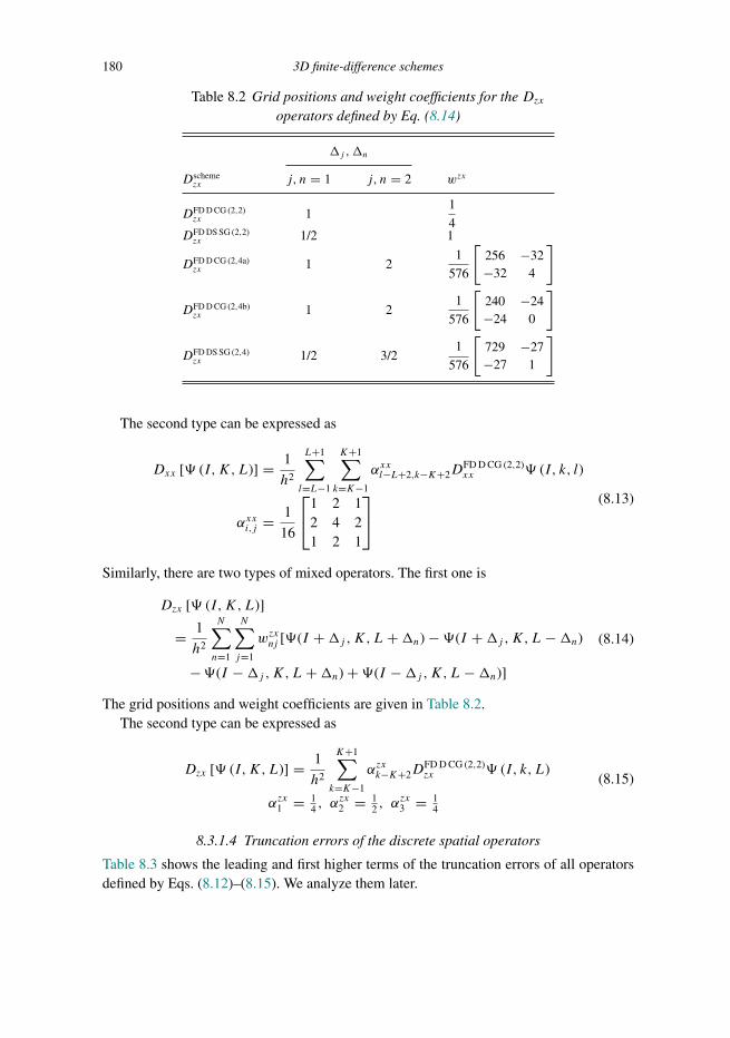
Trim: 247mm × 174mm Top: 14.762mm Gutter: 23.198mmCUUK2497-08 CUUK2497/Moczo ISBN: 978 1 107 02881 4 November 16, 2013 8:50
180 3D finite-difference schemes
Table 8.2 Grid positions and weight coefficients for the Dzxoperators defined by Eq. (8.14)
�j,�n
Dschemezx j, n = 1 j, n = 2 wzx
DFD D CG (2,2)zx 1
1
4DFD DS SG (2,2)zx 1/2 1
DFD D CG (2,4a)zx 1 2
1
576
[256 −32−32 4
]
DFD D CG (2,4b)zx 1 2
1
576
[240 −24−24 0
]
DFD DS SG (2,4)zx 1/2 3/2
1
576
[729 −27−27 1
]
The second type can be expressed as
Dxx [� (I,K,L)] = 1
h2
L+1∑l=L−1
K+1∑k=K−1
αxxl−L+2,k−K+2DFD D CG (2,2)xx � (I, k, l)
αxxi,j = 1
16
⎡⎣1 2 1
2 4 21 2 1
⎤⎦ (8.13)
Similarly, there are two types of mixed operators. The first one is
Dzx [� (I,K,L)]
= 1
h2
N∑n=1
N∑j=1
wzxnj [�(I +�j,K,L+�n) −�(I +�j,K,L−�n)
−�(I −�j,K,L+�n) +�(I −�j,K,L−�n)]
(8.14)
The grid positions and weight coefficients are given in Table 8.2.The second type can be expressed as
Dzx [� (I,K,L)] = 1
h2
K+1∑k=K−1
αzxk−K+2DFD D CG (2,2)zx � (I, k, L)
αzx1 = 14 , α
zx2 = 1
2 , αzx3 = 1
4
(8.15)
8.3.1.4 Truncation errors of the discrete spatial operators
Table 8.3 shows the leading and first higher terms of the truncation errors of all operatorsdefined by Eqs. (8.12)–(8.15). We analyze them later.

Trim: 247mm × 174mm Top: 14.762mm Gutter: 23.198mmCUUK2497-08 CUUK2497/Moczo ISBN: 978 1 107 02881 4 November 16, 2013 8:50
8.3 Accuracy with respect to P-wave to S-wave ratio 181
Table 8.3 The leading and 1st higher terms of the truncation errors of the nonmixed andmixed spatial operators defined by Eqs. (8.12)–(8.15). (a) 2nd-order operators,
(b) 4th-order operators
(a)Operator truncation error ×20160
DFD D CG (2,2)xx
1680� (4,0,0)h2
+ 56� (6,0,0)h4
DFD D CG (2,2)zx
6720(
12�
(1,0,3) + 12�
(3,0,1))h2
+ 896(
316�
(1,0,5) + 1016�
(3,0,3) + 316�
(5,0,1))h4
DFD DS PSG (2,2)xx
11760(
37�
(2,0,2) + 17�
(4,0,0) + 37�
(2,2,0))h2
+ 2996(
1107
(2� (6,0,0) + 15� (4,2,0) + 15� (4,0,2) + 15� (2,4,0) + 45� (2,2,2) + 15� (2,0,4)
))h4
DFD DS PSG (2,2)zx
11760(
27�
(1,0,3) + 37�
(1,2,1) + 27�
(3,0,1))h2
+ 2996(
1107
(6� (1,0,5) + 30� (1,2,3) + 15� (1,4,1) + 20� (3,0,3) + 30� (3,2,1) + 6� (5,0,1)
))h4
DFD DS SG (2,2)xx
1680� (4,0,0)h2
+ 56� (6,0,0)h4
DFD DS SG (2,2)zx
1680(
12�
(1,0,3) + 12�
(3,0,1))h2
+ 56(
316�
(1,0,5) + 1016�
(3,0,3) + 316�
(5,0,1))h4
(b)Operator truncation error ×20160
DFD D CG (2,4a)xx
− 1344� (6,0,0)h4
− 300� (8,0,0)h6
DFD D CG (2,4a)zx
− 1344(
12�
(1,0,5) + 12�
(5,0,1))h4
− 160(
12�
(1,0,7) + 12�
(7,0,1))h6
DFD D CG (2,4b)xx
− 224� (6,0,0)h4
− 20� (8,0,0)h6
DFD D CG (2,4b)zx
− 1904(
617�
(1,0,5) + 517�
(3,0,3) + 617�
(5,0,1))h4
− 440(
422�
(1,0,7) + 722�
(3,0,5) + 722�
(5,0,3) + 422�
(7,0,1))h6
DFD DS SG (2,4)xx
− 189� (6,0,0)h4
− 454 �
(8,0,0)h6
DFD DS SG (2,4)zx
− 189(
12�
(1,0,5) + 12�
(5,0,1))h4
− 454
(12�
(1,0,7) + 12�
(7,0,1))h6
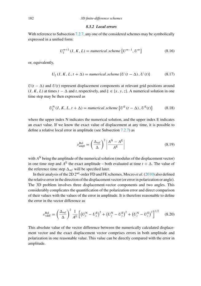
Trim: 247mm × 174mm Top: 14.762mm Gutter: 23.198mmCUUK2497-08 CUUK2497/Moczo ISBN: 978 1 107 02881 4 November 16, 2013 8:50
182 3D finite-difference schemes
8.3.2 Local errors
With reference to Subsection 7.2.7, any one of the considered schemes may be symbolicallyexpressed in a unified form:
Um+1ξ (I,K,L) = numerical scheme
{Um−1, Um
}(8.16)
or, equivalently,
Uξ (I,K,L, t +�) = numerical scheme {U (t −�) , U (t)} (8.17)
U (t −�) and U (t) represent displacement components at relevant grid positions around(I,K,L) at times t −� and t, respectively, and ξ ∈ {x, y, z}. A numerical solution in onetime step may be then expressed as
UNξ (I,K,L, t +�) = numerical scheme
{UE (t −�) , UE(t)
}(8.18)
where the upper index N indicates the numerical solution, and the upper index E indicatesan exact value. If we know the exact value of displacement at any time, it is possible todefine a relative local error in amplitude (see Subsection 7.2.7) as
εRelampl =
(�ref
�
)2 ∣∣∣∣AN − AE
AE
∣∣∣∣ (8.19)
withAN being the amplitude of the numerical solution (modulus of the displacement vector)in one time step and AE the exact amplitude – both evaluated at time t +�. The value ofthe reference time step �ref will be specified later.
In their analysis of the 2D 2nd-order FD and FE schemes, Moczo et al. (2010) also definedthe relative error in the direction of the displacement vector (or error in polarization or angle).The 3D problem involves three displacement-vector components and two angles. Thisconsiderably complicates the quantification of the polarization error and direct comparisonof their values with the values of the error in amplitude. It is therefore reasonable to definethe error in the vector difference as
εRelvdiff =
(�ref
�
)2 1
AE
[(UNx − UE
x
)2 + (UNy − UE
y
)2 + (UNz − UE
z
)2]1/2
(8.20)
This absolute value of the vector difference between the numerically calculated displace-ment vector and the exact displacement vector comprises errors in both amplitude andpolarization in one reasonable value. This value can be directly compared with the error inamplitude.

Trim: 247mm × 174mm Top: 14.762mm Gutter: 23.198mmCUUK2497-08 CUUK2497/Moczo ISBN: 978 1 107 02881 4 November 16, 2013 8:50
8.3 Accuracy with respect to P-wave to S-wave ratio 183
ϕ
δ
xx
yy
z
z
δϕ
u
uk
Figure 8.3 Cartesian coordinate system, angles ϕ and δ for defining a direction of propagation,displacement vector and displacement components of the plane S-wave.
8.3.3 The exact and numerical values of displacement in a grid
Consider a harmonic plane S wave propagating in an unbounded homogeneous elasticisotropic medium as the exact solution in definitions of the local errors. Assuming a har-monic plane S wave polarized in a vertical plane determined by the z-axis and wavenumbervector �k, the displacement components are
uξ (x, y, z, t ;ω;ϕ, δ) = AξEtExEyEz; ξ ∈ {x, y, z} (8.21)
where
Et = exp [−iωt]Ex = exp [ikxx] Ey = exp
[ikyy
]Ez = exp [ikzz]
kx = k cosϕ sin δ ky = k sinϕ sin δ kz = k cos δAx = A cosϕ cos δ Ay = A sinϕ cos δ Az = −A sin δ
(8.22)
k = ω/β, 0 ≤ δ ≤ π, 0 ≤ ϕ ≤ 2π
ω is the angular frequency, k = |�k| is the wavenumber, δ is the angle between the positivez-axis and the wavenumber vector �k (the direction of propagation), ϕ is the angle betweenthe positive x-axis and the vertical plane determined by the z-axis and wavenumber vector�k; see Fig. 8.3. The restriction to the S wave is reasonable: numerical modelling of P-wavepropagation poses a minor problem if the modelling comprises both types of waves. Wewill explain why this is so later. Note that the sign convention in Eqs. (8.22) is consistentwith that used by Moczo et al. (2011).
Recalling spatial sampling Nλ = λ/h, Eq. (7.34), wavenumber k may be expressed as
k = ω/β = 2π/(hNλ) (8.23)

Trim: 247mm × 174mm Top: 14.762mm Gutter: 23.198mmCUUK2497-08 CUUK2497/Moczo ISBN: 978 1 107 02881 4 November 16, 2013 8:50
184 3D finite-difference schemes
and
kxh = 2π
Nλcosϕ sin δ, kyh = 2π
Nλsinϕ sin δ, kzh = 2π
Nλcos δ (8.24)
ω = 2πβ/(hNλ) (8.25)
Considering the stability condition for any of the numerical schemes in the form � ≤� (h, α, β) and the stability ratio p = �/�; 0 < p ≤ 1, the time step�may be expressedas
� = p� (h, α, β) (8.26)
Without loss of generality, consider
xI = 0, yK = 0, zL = 0, tm = 0
and evaluate errors at
xI = 0, yK = 0, zL = 0, tm+1 = � (8.27)
The real exact displacement at this space–time grid position is, see Eqs. (8.21) and (8.22),
Re{uξ (0, 0, 0,�)
} = Aξ cos (ω�) (8.28)
and the exact amplitude is
AE = ([Ax cos(ω�)]2 + [Ay cos(ω�)]2 + [Az cos(ω�)]2)1/2 = A|cos(ω�)| (8.29)
The exact values of (complex) displacements entering the r.h.s. of schemes (8.11) areevaluated as
Um−1ξ (I,K,L) = uξ (0, 0, 0, t = −�;ω;ϕ, δ) = Aξ exp[+iω�]Umξ (I,K,L) = uξ (0, 0, 0, t = 0;ω;ϕ, δ) = Aξ
Umξ (I +�I ,K +�K,L+�L) = uξ (h�I , h�K, h�L, t = 0;ω;ϕ, δ)= Aξ exp[+ikxh�I ] exp[+ikyh�K ] exp[+ikzh�L]
(8.30)
The grid-index increments�I ,�K and�L depend on a numerical scheme. Quantities kxh,kyh and kzh are given by Eq. (8.24).
According to Eqs. (8.11)–(8.15), each scheme effectively includes the second powerof quantity (β/h)�. Quantities ω�, (β/h)� and � entering the numerical schemes andformulas for the errors are summarized in Table 8.4.Um+1x , Um+1
y and Um+1z , evaluated at (I,K,L), are obtained using schemes (8.11). The
amplitude of the numerical solution is then
AN =([
Re{Um+1x
}]2 + [Re{Um+1y
}]2 + [Re{Um+1z
}]2)1/2
(8.31)
In principle, any time step may be chosen as a reference time step�ref appearing in formulas(7.104) and (8.20) for the errors. One reasonable choice is �ref = � for FD DS SG (2,4);p = 0.9, Nλ = 6, r = 1.42. The reason for FD DS SG (2,4) will become clear later;Nλ = 6is the most common choice for the spatial sampling in the numerical modelling of earthquake
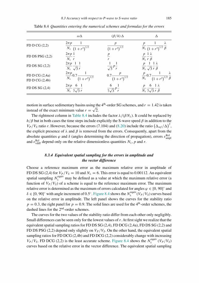
Trim: 247mm × 174mm Top: 14.762mm Gutter: 23.198mmCUUK2497-08 CUUK2497/Moczo ISBN: 978 1 107 02881 4 November 16, 2013 8:50
8.3 Accuracy with respect to P-wave to S-wave ratio 185
Table 8.4 Quantities entering the numerical schemes and formulas for the errors
ω� (β/h)� �
FD D CG (2,2)2πp
Nλ
1(1 + r2
)1/2
p(1 + r2
)1/2
p
Nλ
1(1 + r2
)1/2
λ
β
FD DS PSG (2,2)2πp
Nλ
1
r
p
r
p
Nλ
1
r
λ
β
FD DS SG (2,2)2πp
Nλ
1√3
1
r
1√3p
1
r
p
Nλ
1√3
1
r
λ
β
FD D CG (2,4a)FD D CG (2,4b)
2πp
Nλ0.7
1(1 + r2
)1/2 0.7p(
1 + r2)1/2
p
Nλ0.7
1(1 + r2
)1/2
λ
β
FD DS SG (2,4)2πp
Nλ
6
7√
3
1
r
6
7√
3p
1
r
p
Nλ
6
7√
3
1
r
λ
β
motion in surface sedimentary basins using the 4th-order SG schemes, and r = 1.42 is takeninstead of the exact minimum value r = √
2.The rightmost column in Table 8.4 includes the factor λ/(βNλ). It could be replaced by
h/β but in both cases the time steps include explicitly the S-wave speed β in addition to theVP /VS ratio r. However, because the errors (7.104) and (8.20) include the ratio
(�ref /�
)2,
the explicit presence of λ and β is removed from the errors. Consequently, apart from theabsolute quantities ϕ and δ (angles determining the direction of propagation), errors εRel
ampl
and εRelvdiff depend only on the relative dimensionless quantities Nλ, p and r.
8.3.4 Equivalent spatial sampling for the errors in amplitude andthe vector difference
Choose a reference maximum error as the maximum relative error in amplitude ofFD DS SG (2,4) for VP /VS = 10 andNλ = 6. This error is equal to 0.00112. An equivalentspatial sampling N equiv
λ may be defined as a value at which the maximum relative error (afunction of VP /VS) of a scheme is equal to the reference maximum error. The maximumrelative error is determined as the maximum of errors calculated for angles ϕ ∈ [0, 90]◦ andδ ∈ [0, 90]◦ with angle increment of 0.5◦. Figure 8.4 shows theN equiv
λ (VP /VS) curves basedon the relative error in amplitude. The left panel shows the curves for the stability ratiop = 0.3, the right panel for p = 0.9. The solid lines are used for the 4th-order schemes, thedashed lines for the 2nd-order schemes.
The curves for the two values of the stability ratio differ from each other only negligibly.Small differences can be seen only for the lowest values of r. At first sight we realize that theequivalent spatial sampling ratios for FD DS SG (2,4), FD DCG (2,4a), FD DS SG (2,2) andFD DS PSG (2,2) depend only slightly on VP /VS . On the other hand, the equivalent spatialsampling ratios for FD DCG (2,4b) and FD DCG (2,2) considerably change with increasingVP /VS . FD DCG (2,2) is the least accurate scheme. Figure 8.4 shows the N equiv
λ (VP /VS)curves based on the relative error in the vector difference. The equivalent spatial sampling
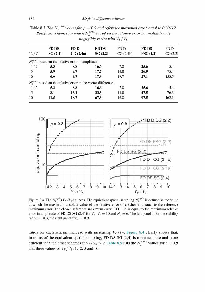
Trim: 247mm × 174mm Top: 14.762mm Gutter: 23.198mmCUUK2497-08 CUUK2497/Moczo ISBN: 978 1 107 02881 4 November 16, 2013 8:50
186 3D finite-difference schemes
Table 8.5 The N equivλ values for p = 0.9 and reference maximum error equal to 0.00112.
Boldface: schemes for which N equivλ based on the relative error in amplitude only
negligibly varies with VP /VS
VP /VS
FD DSSG (2,4)
FD DCG (2,4a)
FD DSSG (2,2)
FD DCG (2,4b)
FD DSPSG (2,2)
FD DCG (2,2)
Nequivλ based on the relative error in amplitude
1.42 5.3 8.8 16.6 7.8 25.6 15.45 5.9 9.7 17.7 14.0 26.9 75.4
10 6.0 9.7 17.8 19.7 27.1 153.5
Nequivλ based on the relative error in the vector difference
1.42 5.3 8.8 16.6 7.8 25.6 15.45 8.1 13.1 33.3 14.0 47.5 76.3
10 11.5 18.7 67.3 19.8 97.5 162.1
1.4 2 3 4 5 6 7 8 9 10
FD D CG (2,2)p = 0.9
FD DS SG (2,4)
FD D CG (2,4a)
FD DS SG (2,2)
FD DS PSG (2,2)
FD D CG (2,4b)
1.4 2 3 4 5 6 7 8 9 10
10
100p = 0.3
equi
vale
ntsa
mpl
ing
/P SV V/P SV V
Figure 8.4 The N equivλ (VP /VS) curves. The equivalent spatial sampling N equiv
λ is defined as the valueat which the maximum absolute value of the relative error of a scheme is equal to the referencemaximum error. The chosen reference maximum error, 0.00112, is equal to the maximum relativeerror in amplitude of FD DS SG (2,4) for VP�VS = 10 and Nλ = 6. The left panel is for the stabilityratio p = 0.3, the right panel for p = 0.9.
ratios for each scheme increase with increasing VP /VS . Figure 8.4 clearly shows that,in terms of the equivalent spatial sampling, FD DS SG (2,4) is more accurate and moreefficient than the other schemes if VP /VS > 2. Table 8.5 lists the N equiv
λ values for p = 0.9and three values of VP /VS : 1.42, 5 and 10.
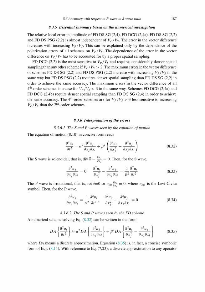
Trim: 247mm × 174mm Top: 14.762mm Gutter: 23.198mmCUUK2497-08 CUUK2497/Moczo ISBN: 978 1 107 02881 4 November 16, 2013 8:50
8.3 Accuracy with respect to P-wave to S-wave ratio 187
8.3.5 Essential summary based on the numerical investigation
The relative local error in amplitude of FD DS SG (2,4), FD DCG (2,4a), FD DS SG (2,2)and FD DS PSG (2,2) is almost independent of VP /VS . The error in the vector differenceincreases with increasing VP /VS . This can be explained only by the dependence of thepolarization errors of all schemes on VP /VS . The dependence of the error in the vectordifference on VP /VS has to be accounted for by a proper spatial sampling.
FD DCG (2,2) is the most sensitive to VP /VS and requires considerably denser spatialsampling than any other scheme ifVP /VS > 2. The maximum errors in the vector differenceof schemes FD DS SG (2,2) and FD DS PSG (2,2) increase with increasing VP /VS in thesame way but FD DS PSG (2,2) requires denser spatial sampling than FD DS SG (2,2) inorder to achieve the same accuracy. The maximum errors in the vector difference of all4th-order schemes increase for VP /VS > 3 in the same way. Schemes FD DCG (2,4a) andFD DCG (2,4b) require denser spatial sampling than FD DS SG (2,4) in order to achievethe same accuracy. The 4th-order schemes are for VP /VS > 3 less sensitive to increasingVP /VS than the 2nd-order schemes.
8.3.6 Interpretation of the errors
8.3.6.1 The S and P waves seen by the equation of motion
The equation of motion (8.10) in concise form reads
∂2ui
∂t2= α2 ∂
2uj
∂xj ∂xi+ β2
(∂2ui
∂x2j
− ∂2uj
∂xj ∂xi
)(8.32)
The S wave is solenoidal, that is, div �u = ∂uj∂xj
= 0. Then, for the S wave,
∂2uj
∂xj ∂xi= 0,
∂2ui
∂x2j
− ∂2uj
∂xj ∂xi= 1
β2
∂2ui
∂t2(8.33)
The P wave is irrotational, that is, rot �u=0 or εkji∂ui∂xj
= 0, where εkji is the Levi-Civitasymbol. Then, for the P wave,
∂2uj
∂xj ∂xi= 1
α2
∂2ui
∂t2,∂2ui
∂x2j
− ∂2uj
∂xj ∂xi= 0 (8.34)
8.3.6.2 The S and P waves seen by the FD scheme
A numerical scheme solving Eq. (8.32) can be written in the form
DA
{∂2ui
∂t2
}≈ α2DA
{∂2uj
∂xj ∂xi
}+ β2DA
{∂2ui
∂x2j
− ∂2uj
∂xj∂xi
}(8.35)
where DA means a discrete approximation. Equation (8.35) is, in fact, a concise symbolicform of Eqs. (8.11). With reference to Eq. (7.23), a discrete approximation to any operator

Trim: 247mm × 174mm Top: 14.762mm Gutter: 23.198mmCUUK2497-08 CUUK2497/Moczo ISBN: 978 1 107 02881 4 November 16, 2013 8:50
188 3D finite-difference schemes
in general can be expressed as a sum of the exact differential operator and a truncation error(for which we will use symbol TrunErr). Equation (8.35) can be then written as
∂2ui
∂t2+ TrunErr
{∂2ui
∂t2
}≈ α2
(∂2uj
∂xj ∂xi+ TrunErr
{∂2uj
∂xj ∂xi
})(8.36)
+β2
(∂2ui
∂x2j
− ∂2uj
∂xj ∂xi+ TrunErr
{∂2ui
∂x2j
− ∂2uj
∂xj ∂xi
})
The harmonic plane S wave Considering the first of Eqs. (8.33), equality ∂2uSi∂t2
= −ω2uSi ,and the fact that each 2nd spatial derivative of a displacement-vector component is propor-tional to −ω2uSi /β
2, Eq. (8.36) may be written as
(1 + error tSi
) (−ω2uSi) ≈ α2
(0 + error αSi
) (−ω2uSi)β2 +
(1 + error βSi
) (−ω2uSi)
(8.37)
and eventually
uSi ≈(r2error αSi + 1 + error βSi − error tSi
)uSi (8.38)
The double-index summation rule does not apply to index i in Eqs. (8.37)–(8.51).The error terms
error αSi =β2TrunErr
{∂2uSj
∂xj ∂xi
}
−ω2uSi,
error βSi =β2TrunErr
{∂2uSi
∂x2j
− ∂2uSj
∂xj ∂xi
}
−ω2uSi
(8.39)
do not depend on r, that is, VP /VS . However, the error term error tSi does depend on r:
error tSi =TrunErr
{∂2uSi∂t2
}−ω2uSi
= c11
r2+ c2
1
r4+ · · · (8.40)
Coefficients cl ; l = 1, 2, . . . do not depend on r. Note that the series in powers of 1/r2 isdue to the 2nd-order approximation to the 2nd temporal derivative. The squares of the timestep, �2, are expressed using 1/r2.
The harmonic plane P wave Considering the second of Eqs. (8.34), equality ∂2uPi∂t2
=−ω2uPi , and the fact that each 2nd spatial derivative of a displacement-vector component is

Trim: 247mm × 174mm Top: 14.762mm Gutter: 23.198mmCUUK2497-08 CUUK2497/Moczo ISBN: 978 1 107 02881 4 November 16, 2013 8:50
8.3 Accuracy with respect to P-wave to S-wave ratio 189
proportional to −ω2uPi /α2, Eq. (8.36) may be written as
(1 + error tPi
) (−ω2uPi) ≈ (
1 + error αPi) (−ω2uPi
)+ β2(
0 + error βPi
) (−ω2uPi)/α2
(8.41)
and eventually
uPi ≈(
1 + error αPi + 1
r2error βPi − error tPi
)uPi (8.42)
Analogously to the error terms in Eqs. (8.39), error αPi and error βPi do not depend on r.The dependence of error tPi on r is analogous to that of error tSi in Eq. (8.40).
Essential comparison of the P and S waves There is an important difference betweenEq. (8.38) for the S wave and Eq. (8.42) for the P wave: whereas r2error αSi increases withincreasing VP /VS , 1
r2 error βPi decreases with increasing VP /VS . This is why a large valueof VP /VS does not pose a problem for the P wave.
8.3.6.3 Structure of the errors in amplitude and vector difference
Because we restrict our further discussion to the S wave, in the following section we willomit explicit indication of the S wave in the displacement-vector components and errorterms. Recall Eq. (8.35). The analyzed schemes differ from each other by the approximationson the r.h.s. They share the same approximation to the 2nd time derivative:
DA
{∂2ui
∂t2
}≈ 1
�2
(um+1i − 2umi + um−1
i
)(8.43)
Using Eq. (8.43) in Eq. (8.35) we can get the scheme for the numerical displacementcomponent at the time level m+ 1 in the form
Num+1i = 2umi − um−1
i +�2
(α2DA
{∂2uj
∂xj∂xi
}+ β2DA
{∂2ui
∂x2j
− ∂2uj
∂xj ∂xi
})(8.44)
Recalling the concept of the local error, Eqs. (8.16)–(8.20), we distinguish the numericalvalue, labelled N, on the l.h.s., from the exact values of the displacement components on ther.h.s. (not labelled). Subtracting um+1
i from both sides of Eq. (8.44), dividing the equationby �2, and using Eq. (8.43), we obtain
(Num+1i − um+1
i
) 1
�2= −DA
{∂2ui
∂t2
}+ α2DA
{∂2uj
∂xj ∂xi
}+ β2DA
{∂2ui
∂x2j
− ∂2uj
∂xj ∂xi
}
(8.45)

Trim: 247mm × 174mm Top: 14.762mm Gutter: 23.198mmCUUK2497-08 CUUK2497/Moczo ISBN: 978 1 107 02881 4 November 16, 2013 8:50
190 3D finite-difference schemes
Each of the discrete approximations on the r.h.s. can be replaced by the sum of the exactoperator and truncation error. Then,
(Num+1i − um+1
i
) 1
�2= −∂
2ui
∂t2+ α2 ∂
2uj
∂xj∂xi+ β2
(∂2ui
∂x2j
− ∂2uj
∂xj ∂xi
)− TrunErr
{∂2ui
∂t2
}
+α2TrunErr
{∂2uj
∂xj ∂xi
}+ β2TrunErr
{∂2ui
∂x2j
− ∂2uj
∂xj ∂xi
}
(8.46)
The sum of the first three terms on the r.h.s. is equal to zero, see Eq. (8.32), and thus
(Num+1i − um+1
i
) 1
�2= −TrunErr
{∂2ui
∂t2
}+ α2TrunErr
{∂2uj
∂xj ∂xi
}
+β2TrunErr
{∂2ui
∂x2j
− ∂2uj
∂xj∂xi
} (8.47)
Considering Eqs. (8.39) and (8.40)
(Num+1i − um+1
i
) 1
�2=(
error tSi − r2error αSi − error βSi
)ω2ui (8.48)
Referring to definition (8.20) of the error in the vector difference and Eq. (8.29), consideran auxiliary error-component term
εi,vdiff =(
Num+1i − um+1
i
)AE
1
�2=(
error tSi − r2error αSi − error βSi
) ω2ui
|A cosω�|(8.49)
Referring now to definition (8.19) of the error in amplitude and Eq. (8.29), we rearrangeEq. (8.49) and consider another auxiliary error-component term:
εi,ampl =Num+1i
AE
1
�2=(
error tSi − r2error αSi − error βSi
) ω2ui
|A cosω�| + um+1i
|A cosω�|1
�2
(8.50)
Equations (8.21) and (8.22) imply um+1i = ui (t +�) = exp [−iω�] ui(t) and, conse-
quently,
εi,ampl =Num+1i
AE
1
�2=(
error tSi − r2error αSi − error βSi + exp [−iω�]
(ω�)2
)ω2ui
|A cosω�|(8.51)
Errors (7.104) and (8.20) can then be expressed as
εRelampl = (
�ref)2∣∣∣∣[ε2
x,ampl + ε2y,ampl + ε2
z,ampl
]1/2− 1
∣∣∣∣ (8.52)
εRelvdiff = (
�ref)2 [ε2x,vdiff + ε2
y,vdiff + ε2z,vdiff
]1/2(8.53)

Trim: 247mm × 174mm Top: 14.762mm Gutter: 23.198mmCUUK2497-08 CUUK2497/Moczo ISBN: 978 1 107 02881 4 November 16, 2013 8:50
8.3 Accuracy with respect to P-wave to S-wave ratio 191
Table 8.6 Comparison of coefficients of the leading and 1st higherterms of the truncation errors TrunErr {Dxx} and TrunErr {Dzx}.(a) Schemes with the error in amplitude almost independent of
VP /VS . (b) Schemes with the error in amplitude dependent on VP /VS
2nd-order schemes 4th-order schemes
CLT CLT
Operator C1HT Operator C1HT
(a)DFD DS SG 2xx c2 DFD DS SG 4
xx d4
1 c4 1 d6
DFD DS SG 2zx 1 c2 DFD DS SG 4
zx 1 d4
c4 d6
DFD DS PSG 2xx 7.0c2 DFD D CG 4a
xx 7.1d4
1 53.5c4 1 26.7d6
DFD DS PSG 2zx 1 7.0c2 DFD D CG 4a
zx 0.53 7.1d4
53.5c4 14.2d6
(b)
DFD D CG 2xx c2 DFD D CG 4b
xx 1.2d4
4 c4 8.5 1.8d6
DFD D CG 2zx 16 4.0c2 DFD D CG 4b
zx 22 10.1d4
16.0c4 39.1d6
Difference between εRelampl and εRel
vdiff Obviously, the auxiliary error-component terms εi,ampl
and εi,vdiff do not quantitatively represent the entire values of εRelampl and εRel
vdiff , respectively.They do, however, indicate where the difference between εRel
ampl and εRelvdiff comes from.
The r.h.s of Eqs. (8.49) and (8.51) differ by the 4th term in the parenthesis in Eq. (8.51).The absolute value of this term is proportional to r2, see Table 8.4. The fact that εRel
ampl ofschemes FD DS SG (2,4), FD DCG (2,4a), FD DS SG (2,2) and FD DS PSG (2,2) is almostindependent of r is likely related to the interaction of the 2nd and 4th terms because they areboth proportional to r2.
8.3.6.4 Truncation errors of the discrete approximations to the 2nd nonmixedand mixed spatial derivatives
It is interesting to look at the structure of the truncation errors of the 2nd-order and 4th-orderoperators for the 2nd mixed and nonmixed derivatives. The errors are shown in Table 8.6.Define ratios for each scheme:
CLT = coeff. of leading term of TrunErr {Dzx}coeff. of leading term of TrunErr {Dxx}
CkHT = coeff. of k-th higher term of TrunErr {Dzx}coeff. of k-th higher term of TrunErr {Dxx} ; k = 1, 2, 3, . . .
(8.54)

Trim: 247mm × 174mm Top: 14.762mm Gutter: 23.198mmCUUK2497-08 CUUK2497/Moczo ISBN: 978 1 107 02881 4 November 16, 2013 8:50
192 3D finite-difference schemes
CLT and C1HT are shown in Table 8.6. Table 8.6(a) includes the four schemes for whichεRel
ampl are almost independent of VP /VS ; Table 8.6(b) includes the other schemes. All thefour schemes in Table 8.6(a) have CLT = 1. Schemes FD DS SG (2,4), FD DS SG (2,2)and FD DS PSG (2,2) have also CkHT = 1 (the table shows only the first one). On the otherhand, neither of the two schemes in Table 8.6(b) has CLT or C1HT equal to 1.
We denote by c2 and c4 the coefficients of the leading term and 1st higher term ofTrunErr {Dxx} or TrunErr {Dzx} of the 2nd-order FD DS SG (2,2) operators. The lower indexindicates the power of the grid spacing h. Similarly, denote by d4 and d6 the coefficientsof the leading term and 1st higher term of TrunErr {Dxx} or TrunErr {Dzx} of the 4th-orderFD DS SG (2,4) operators. Table 8.6 shows the corresponding coefficients of other 2nd-orderoperators as multiples of c2 and c4. Similarly, coefficients of the other 4th-order operatorsare shown as multiples of d4 and d6.
In general, for the schemes of the same order (either 2nd or 4th) for given CLT or C1HT ,εRel
ampl and εRelvdiff increase with increasing absolute values of coefficients of terms in the
truncation errors. This is seen well for FD DS SG (2,2) and FD DS PSG (2,2).CLT orC1HT
are the same but the coefficients of terms in the truncation errors are different. It is alsointeresting to compare FD DS SG (2,4) and FD DCG (2,4a). Although they have differentC1HT , the ratio of the coefficients of the leading terms, which is 7.1, well quantifies thedifference in their errors (see Fig. 8.4).
8.3.7 Summary
The relative local error in amplitude, εRelampl, of schemes FD DS SG (2,4), FD DCG (2,4a),
FD DS SG (2,2) and FD DS PSG (2,2) is almost independent of VP /VS . The error inthe vector difference, εRel
vdiff , increases with increasing VP /VS . This can be explained bythe dependence of the polarization errors of all schemes on VP /VS . FD DCG (2,2) is themost sensitive to increasing VP /VS and for VP /VS > 2 requires considerably denser spatialsampling than any other scheme. The 4th-order schemes for VP /VS > 3 are less sensitive toincreasing VP /VS than the 2nd-order schemes. The maximum εRel
vdiff of all 4th-order schemesincrease with increasing VP /VS for VP /VS > 3 in the same way. FD DCG (2,4a) andFD DCG (2,4b) require denser spatial sampling than FD DS SG (2,4) in order to achievethe same accuracy.
FD DS SG (2,4), FD DCG (2,4a), FD DS SG (2,2) and FD DS PSG (2,2) with εRelampl almost
independent of VP /VS have the same coefficients of the leading terms of the truncationerrors of approximations to the 2nd mixed and nonmixed spatial derivatives. None of theother schemes have those coefficients equal.
The general theoretical conclusion is that the homogeneity of the approximations to the2nd mixed and nonmixed spatial derivatives in terms of the coefficients of the leading termsof their truncation errors as well as the absolute values of the coefficients are key factors forthe behaviour of the numerical schemes with increasing VP /VS . The practical conclusionfor the existing schemes is that the dependence of εRel
vdiff on VP /VS should be accounted forby a proper (sufficiently dense) spatial sampling.
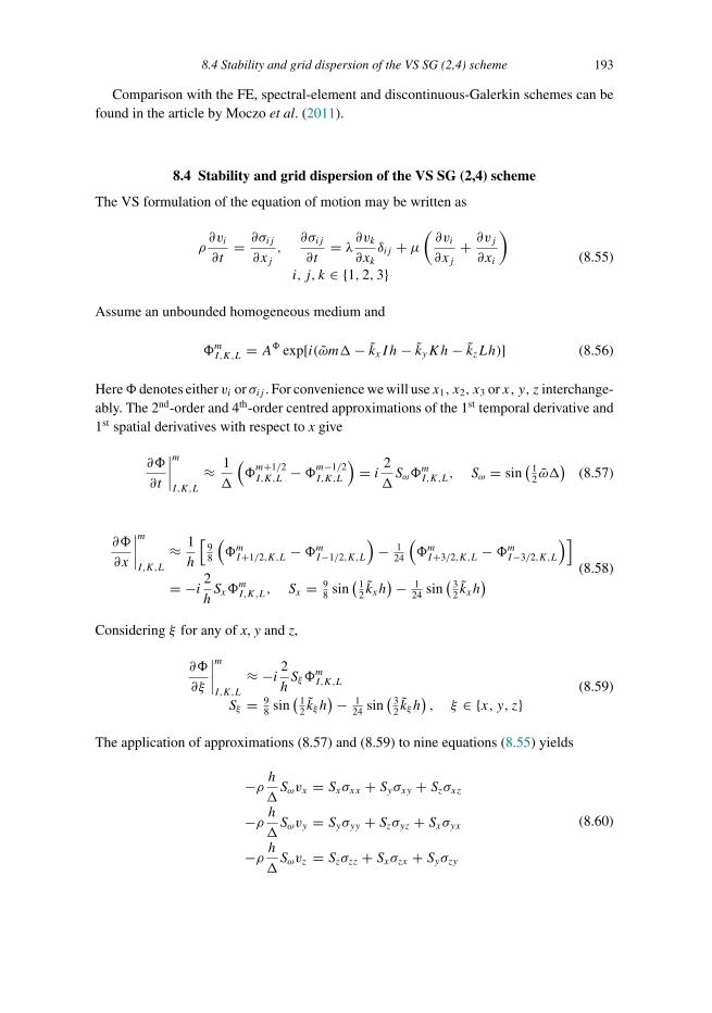
Trim: 247mm × 174mm Top: 14.762mm Gutter: 23.198mmCUUK2497-08 CUUK2497/Moczo ISBN: 978 1 107 02881 4 November 16, 2013 8:50
8.4 Stability and grid dispersion of the VS SG (2,4) scheme 193
Comparison with the FE, spectral-element and discontinuous-Galerkin schemes can befound in the article by Moczo et al. (2011).
8.4 Stability and grid dispersion of the VS SG (2,4) scheme
The VS formulation of the equation of motion may be written as
ρ∂vi
∂t= ∂σij
∂xj,∂σij
∂t= λ∂vk
∂xkδij + μ
(∂vi
∂xj+ ∂vj∂xi
)i, j, k ∈ {1, 2, 3}
(8.55)
Assume an unbounded homogeneous medium and
�mI,K,L = A� exp[i(ωm�− kxIh− kyKh− kzLh)] (8.56)
Here� denotes either vi or σij . For convenience we will use x1, x2, x3 or x, y, z interchange-ably. The 2nd-order and 4th-order centred approximations of the 1st temporal derivative and1st spatial derivatives with respect to x give
∂�
∂t
∣∣∣∣mI,K,L
≈ 1
�
(�m+1/2I,K,L −�m−1/2
I,K,L
)= i 2
�Sω�
mI,K,L, Sω = sin
(12 ω�
)(8.57)
∂�
∂x
∣∣∣∣mI,K,L
≈ 1
h
[98
(�mI+1/2,K,L −�mI−1/2,K,L
)− 1
24
(�mI+3/2,K,L −�mI−3/2,K,L
)]= −i 2
hSx�
mI,K,L, Sx = 9
8 sin(
12 kxh
)− 124 sin
(32 kxh
) (8.58)
Considering ξ for any of x, y and z,
∂�
∂ξ
∣∣∣∣mI,K,L
≈ −i 2hSξ�
mI,K,L
Sξ = 98 sin
(12 kξ h
)− 124 sin
(32 kξ h
), ξ ∈ {x, y, z}
(8.59)
The application of approximations (8.57) and (8.59) to nine equations (8.55) yields
−ρ h�Sωvx = Sxσxx + Syσxy + Szσxz
−ρ h�Sωvy = Syσyy + Szσyz + Sxσyx
−ρ h�Sωvz = Szσzz + Sxσzx + Syσzy
(8.60)
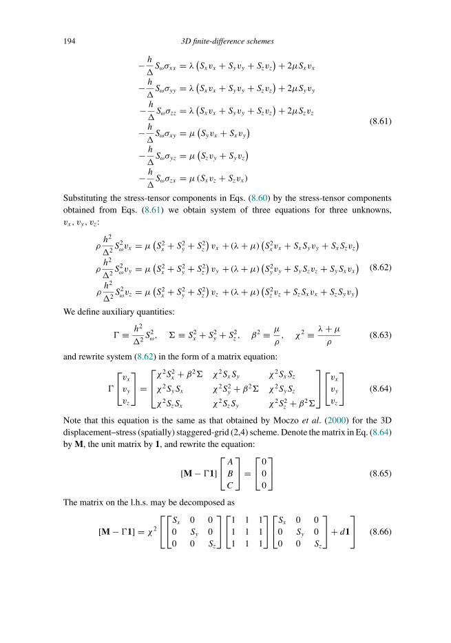
Trim: 247mm × 174mm Top: 14.762mm Gutter: 23.198mmCUUK2497-08 CUUK2497/Moczo ISBN: 978 1 107 02881 4 November 16, 2013 8:50
194 3D finite-difference schemes
− h�Sωσxx = λ (Sxvx + Syvy + Szvz
)+ 2μSxvx
− h�Sωσyy = λ (Sxvx + Syvy + Szvz
)+ 2μSyvy
− h�Sωσzz = λ (Sxvx + Syvy + Szvz
)+ 2μSzvz
− h�Sωσxy = μ (Syvx + Sxvy
)− h�Sωσyz = μ (Szvy + Syvz
)− h�Sωσzx = μ (Sxvz + Szvx)
(8.61)
Substituting the stress-tensor components in Eqs. (8.60) by the stress-tensor componentsobtained from Eqs. (8.61) we obtain system of three equations for three unknowns,vx, vy, vz:
ρh2
�2S2ωvx = μ (S2
x + S2y + S2
z
)vx + (λ+ μ)
(S2xvx + SxSyvy + SxSzvz
)ρh2
�2S2ωvy = μ (S2
x + S2y + S2
z
)vy + (λ+ μ)
(S2yvy + SySzvz + SySxvx
)ρh2
�2S2ωvz = μ (S2
x + S2y + S2
z
)vz + (λ+ μ)
(S2z vz + SzSxvx + SzSyvy
)(8.62)
We define auxiliary quantities:
� ≡ h2
�2S2ω, � ≡ S2
x + S2y + S2
z , β2 ≡ μ
ρ, χ2 ≡ λ+ μ
ρ(8.63)
and rewrite system (8.62) in the form of a matrix equation:
�
⎡⎣vxvyvz
⎤⎦ =
⎡⎢⎣χ2S2
x + β2� χ2SxSy χ2SxSz
χ2SySx χ2S2y + β2� χ2SySz
χ2SzSx χ2SzSy χ2S2z + β2�
⎤⎥⎦⎡⎣vxvyvz
⎤⎦ (8.64)
Note that this equation is the same as that obtained by Moczo et al. (2000) for the 3Ddisplacement–stress (spatially) staggered-grid (2,4) scheme. Denote the matrix in Eq. (8.64)by M, the unit matrix by 1, and rewrite the equation:
[M − �1]
⎡⎣ABC
⎤⎦ =
⎡⎣0
00
⎤⎦ (8.65)
The matrix on the l.h.s. may be decomposed as
[M − �1] = χ2
⎡⎣⎡⎣Sx 0 0
0 Sy 00 0 Sz
⎤⎦⎡⎣1 1 1
1 1 11 1 1
⎤⎦⎡⎣Sx 0 0
0 Sy 00 0 Sz
⎤⎦+ d1
⎤⎦ (8.66)

Trim: 247mm × 174mm Top: 14.762mm Gutter: 23.198mmCUUK2497-08 CUUK2497/Moczo ISBN: 978 1 107 02881 4 November 16, 2013 8:50
8.4 Stability and grid dispersion of the VS SG (2,4) scheme 195
where
d = (β2� − �)/χ2 (8.67)
A nontrivial solution to Eq. (8.65) exists if Det [M − �1] = 0, which may be written as
χ6Det
⎡⎣⎡⎣Sx 0 0
0 Sy 00 0 Sz
⎤⎦⎡⎣1 1 1
1 1 11 1 1
⎤⎦⎡⎣Sx 0 0
0 Sy 00 0 Sz
⎤⎦+ d1
⎤⎦ = 0 (8.68)
and
Det
⎡⎢⎣S2x + d SxSy SxSz
SxSy S2y + d SySz
SxSz SySz S2z + d
⎤⎥⎦ = 0 (8.69)
from which we obtain
d2(S2x + S2
y + S2z
) = 0 (8.70)
Equation (8.70) is satisfied if
S2x + S2
y + S2z = 0 or d = 0 (8.71)
Consequently we obtain two dispersion relations for the 3D VS SG (2,4) scheme. Consid-ering definitions (8.67), (8.63) and (8.57), Eqs. (8.71) imply
sin2(
12 ω�
) = �2
h2α2(S2x + S2
y + S2z
)sin2
(12 ω�
) = �2
h2β2 (S2
x + S2y + S2
z
) (8.72)
where α2 = (λ+ 2μ) /ρ and β2 = μ/ρ are the squares of the P-wave and S-wave speeds,respectively. Compare dispersion relations (8.72) with that in Table 7.4 for the 1D VS SG(2,4) scheme. The two relations correspond to the possibility of two independent waves –P and S waves. Similarly to the analysis in Subsection 7.3.5, we can obtain relations
� ≤ 6
7√
3
h
α, � ≤ 6
7√
3
h
β(8.73)
for P and S waves. If both types of waves propagate in the grid, the condition for the Pwave has to be taken as the joint stability condition because α > β. Defining the stabilityratio p,
p ≡ 7√
3
6
α
h� (8.74)
the condition for the time step may be written as
� = p 6
7√
3
h
α; 0 < p ≤ 1 (8.75)

Trim: 247mm × 174mm Top: 14.762mm Gutter: 23.198mmCUUK2497-08 CUUK2497/Moczo ISBN: 978 1 107 02881 4 November 16, 2013 8:50
196 3D finite-difference schemes
Denoting the grid P and S wave velocities by α and β, respectively, and assuming physicalwavenumbers kα and kβ , in analogy with Eq. (7.222) we obtain from Eqs. (8.72) relationsfor the normalized grid phase velocities:
α
α= 2
αkα�arcsin
[�
hα(S2x + S2
y + S2z
)1/2]
β
β= 2
βkβ�arcsin
[�
hβ(S2x + S2
y + S2z
)1/2] (8.76)
in which we consider the same time step given by (8.75). Equation (8.75) implies
�
hα = p 6
7√
3,�
hβ = p
r
6
7√
3; r = α
β(8.77)
Spatial samplings for P and S waves are
NPλ = λP /h, NSλ = λS/h, NPλ = rNSλ (8.78)
If both types of waves propagate in the grid, NSλ has to be adopted as the joint spatialsampling because, at a given frequency, λP > λS . Because for both types of waves weapply the same time step (for the P wave) and the same spatial sampling (for the S wave),we obtain, in analogy with Eq. (7.226),
2
αkα�= 2
βkβ�= 7
√3
6
rNSλπp
(8.79)
Using Eqs. (8.77) and (8.79) we may rewrite relations (8.76) in the form
α
α= 7
√3
6
rNSλπp
arcsin
[p
6
7√
3
(S2x + S2
y + S2z
)1/2]
β
β= 7
√3
6
rNSλπp
arcsin
[p
r
6
7√
3
(S2x + S2
y + S2z
)1/2] (8.80)
Recall that Sx, Sy, Sz are given by relation (8.59). For the P wave and the S wave we obtain,respectively,
kxh = 2π
rNSλcosϕ sin δ, kyh = 2π
rNSλsinϕ sin δ, kzh = 2π
rNSλcos δ
kxh = 2π
NSλcosϕ sin δ, kyh = 2π
NSλsinϕ sin δ, kzh = 2π
NSλcos δ
(8.81)
where angles ϕ and δ determine the direction of propagation, as shown in Fig. 8.3. Noteagain that the grid dispersion for the analyzed 3D VS SG (2,4) scheme is the same as thegrid dispersion of the 3D displacement–stress (spatially) staggered-grid (2,4) scheme – aspointed out by Moczo et al. (2000), who explicitly analyzed the latter scheme.
The grid dispersion of P and S waves is illustrated in Fig. 8.5 and Fig. 8.6.It is clear from the figures that, due to the larger wavelength of the P wave, propagation
of P waves is modelled by the FD scheme much better than propagation of S waves. We canalso see considerable grid-dispersion anisotropy of S waves: grid dispersion is strongest
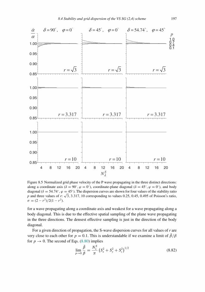
Trim: 247mm × 174mm Top: 14.762mm Gutter: 23.198mmCUUK2497-08 CUUK2497/Moczo ISBN: 978 1 107 02881 4 November 16, 2013 8:50
8.4 Stability and grid dispersion of the VS SG (2,4) scheme 197
αα
90 , 0δ ϕ= = 45 , 0δ ϕ= = 54.74 , 45δ ϕ= =
3r = 3r = 3r =
3.317r = 3.317r = 3.317r =
10r = 10r = 10r =
1.00
0.95
0.90
0.85
1.00
0.95
0.90
0.85
1.00
0.95
0.90
0.854 8 12 16 20
1.00.70.40.1
p
4 8 12 16 20 4 8 12 16 20SNλ
Figure 8.5 Normalized grid phase velocity of the P wave propagating in the three distinct directions:along a coordinate axis (δ = 90◦, ϕ = 0◦), coordinate-plane diagonal (δ = 45◦, ϕ = 0◦), and bodydiagonal (δ = 54.74◦, ϕ = 45◦). The dispersion curves are shown for four values of the stability ratiop and three values of r:
√3, 3.317, 10 corresponding to values 0.25, 0.45, 0.495 of Poisson’s ratio,
σ = (2 − r2)/2(1 − r2).
for a wave propagating along a coordinate axis and weakest for a wave propagating along abody diagonal. This is due to the effective spatial sampling of the plane wave propagatingin the three directions. The densest effective sampling is just in the direction of the bodydiagonal.
For a given direction of propagation, the S-wave dispersion curves for all values of r arevery close to each other for p = 0.1. This is understandable if we examine a limit of β/βfor p → 0. The second of Eqs. (8.80) implies
limp→0
β
β= NSλπ
(S2x + S2
y + S2z
)1/2(8.82)
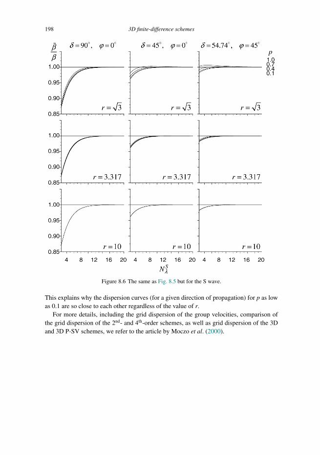
Trim: 247mm × 174mm Top: 14.762mm Gutter: 23.198mmCUUK2497-08 CUUK2497/Moczo ISBN: 978 1 107 02881 4 November 16, 2013 8:50
198 3D finite-difference schemes
Figure 8.6 The same as Fig. 8.5 but for the S wave.
This explains why the dispersion curves (for a given direction of propagation) for p as lowas 0.1 are so close to each other regardless of the value of r.
For more details, including the grid dispersion of the group velocities, comparison ofthe grid dispersion of the 2nd- and 4th-order schemes, as well as grid dispersion of the 3Dand 3D P-SV schemes, we refer to the article by Moczo et al. (2000).

Trim: 247mm × 174mm Top: 14.762mm Gutter: 23.198mmCUUK2497-09 CUUK2497/Moczo ISBN: 978 1 107 02881 4 November 16, 2013 11:36
9
Velocity–stress staggered-grid scheme for anunbounded heterogeneous viscoelastic medium
9.1 FD modelling of a material interface
Models of the Earth’s interior and surface geological structures have to include layers/blocksof different materials. Their contact, the material interface, is a material discontinuityat which material parameters change discontinuously. Assuming a welded interface, theboundary conditions are continuity of the displacement (or particle-velocity) and tractionvector. An apparently natural approach to using the FDM is to apply (a) an FD schemefor the smoothly heterogeneous medium at grid points outside the discontinuity, (b) FDschemes obtained by proper incorporation of the boundary conditions at grid points at ornear the interface. Such an approach has been called homogeneous. Boore (1972b) andKelly et al. (1976) pointed out that a homogeneous FD scheme is specific for a particularproblem. Whereas it is feasible for simple interface geometry, its application to curvedmaterial discontinuities is difficult and therefore had been considered impractical. In anycase, the approach requires a stable and sufficiently accurate FD approximation of theboundary conditions, which is not a trivial problem.
In the alternative heterogeneous approach, only one FD scheme is used for all interiorgrid points (points not lying on the boundaries of a grid) no matter what their positions arewith respect to the material interface. The presence of the interface is accounted for onlyby values of the effective material parameters assigned to grid positions. Therefore, theheterogeneous approach has been much more popular since the beginning of the seventies.
Clearly, a heterogeneous FD scheme should approximate solutions of the equation ofmotion and stress–strain relation valid for both the smoothly heterogeneous medium andthe interface. In fact, the majority of the heterogeneous schemes were developed for smoothmedia and were only intuitively applied to media with material interfaces.
In their pioneering work, Alterman and Karal (1968) used the displacement FD schemeand homogeneous approach for models with simple geometry of the material discon-tinuities. They introduced the concept of fictitious grid points in order to approximateboundary conditions on material discontinuities. Difficulties in application of the homo-geneous approach to curved discontinuities led Boore (1972b) to his explicit continuousstress method. Boore tried to include explicitly a stress-continuity condition on disconti-nuities differently from the homogeneous and heterogeneous approaches. Due to the poor
199
Trim: 247mm × 174mm Top: 14.762mm Gutter: 23.198mmCUUK2497-09 CUUK2497/Moczo ISBN: 978 1 107 02881 4 November 16, 2013 11:36
200 VS SG scheme for unbounded heterogeneous viscoelastic medium
numerical properties of the method Boore (1972b) applied the heterogeneous approach inhis SH modelling. In order to follow variations of the torsion modulus and, at the sametime, to avoid the differentiation of the modulus, he used the mathematical trick givenby Tikhonov and Samarskii (see Subsection 7.3.1) and calculated effective grid moduli asintegral harmonic averages along a grid line between two neighbouring grid points. Ilanet al. (1975) and Ilan and Loewenthal (1976) solved the P-SV problem on the horizontal andvertical planar discontinuities with a homogeneous approach. Instead of the fictitious gridpoints they used Taylor expansions of displacement to couple the equation of motion withthe boundary conditions. Kelly et al. (1976) presented their heterogeneous P-SV schemeswith simple intuitive averaging of material parameters. They compared the heterogeneousand homogeneous formulations using numerical tests and showed unacceptable differencesbetween the two approaches in the case of the corner-edge model. Kummer and Behle(1982) followed the approach of Ilan et al. (1975) and derived the 2nd-order SH schemesfor different types of grid points lying on a step-like polygonal interface between twohomogeneous blocks.
The breakthrough velocity–stress staggered-grid schemes introduced to seismic-wavepropagation modelling by Virieux (1984, 1986) were significant for modelling interfaces.His 2D P-SV scheme did not suffer from stability problems caused by large VP /VS (orPoisson’s ratio) values, which was the case for all displacement schemes on conventionalgrids. Although Virieux did not describe determination of the material grid parameters inhis heterogeneous 2nd-order SH and P-SV velocity–stress schemes, his numerical resultswere sufficiently accurate at the time. Virieux also discussed the discrepancy between thehomogeneous and heterogeneous formulations found by Kelly et al. (1976). He found itdifficult to explain the features of the homogeneous solution.
Fornberg (1988b) suggested using a boundary-conforming grid in order to avoid artificialdiffraction at a staircase interface. An attempt to incorporate internal boundary conditionsinto a displacement FD scheme was made by Sochacki et al. (1991), who a priori assumedvalidity of the equation of motion at the discontinuity and integrated it over a grid cell.Then they FD-approximated the integrated equation of motion. Cunha (1993) developeda modified staggered-grid scheme with short operators for computing derivatives of dis-continuous material properties and long operators for computing derivatives of the fieldvariables. Zahradnık and Priolo (1995) explicitly pointed out the problem of justification ofthe heterogeneous FD schemes and a heterogeneous formulation of the equation of motion.Assuming discontinuous material parameters in the equation of motion, they obtained anexpression whose dominant term is equivalent to the traction continuity condition. Graves(1996) intuitively suggested a formula for determination of effective material grid param-eters in the 3D (2,4) VS SG scheme. Graves was probably the first to explicitly and clearlyexplain the determination of the grid parameters in his scheme. Zhang and Symes (1998)developed a 2D 4th-order full-stencil immersed interface technique to account for a curvedmaterial discontinuity. In the first step, all grid points are solved using a standard FDscheme. In the second step, each grid point whose stencil includes grid points from bothsides of the discontinuity is recalculated using the previous time step’s values with a special

Trim: 247mm × 174mm Top: 14.762mm Gutter: 23.198mmCUUK2497-09 CUUK2497/Moczo ISBN: 978 1 107 02881 4 November 16, 2013 11:36
9.1 FD modelling of a material interface 201
25-point scheme determined using local boundary conditions. Lombard and Piraux (2004)presented an explicit simplified interface method for 2D velocity–stress modelling.
Equivalent medium consistent with the interface boundary conditions It seems thatmany developers of the heterogeneous schemes were not aware of the work by Backus(1962), Schoenberg and Muir (1989) and Muir et al. (1992), or they did not realize themeaning of the work for the development of the heterogeneous schemes. Backus (1962)investigated the long-wave equivalent of a finely layered medium. He showed that a homoge-neous transversely isotropic medium described by five elastic coefficients is the long-waveequivalent of a stack of homogeneous isotropic layers. The coefficients of the equivalentmedium are obtained by a proper averaging of the Lame coefficients of the layers. Theaveraging is consistent with boundary conditions at the interfaces between layers. Backusalso found the long-wave equivalent of a stack of transversely isotropic layers. Schoenbergand Muir (1989) extended the Backus approach to arbitrary anisotropic layers and showedhow an equivalent, homogeneous, anisotropic medium can be constructed from the layeredmedium. In other words, both Backus (1962) and Schoenberg and Muir (1989) found thestress–strain relation for an averaged medium consistent with the interface boundary con-ditions. Neither of them explicitly mentioned FD modelling. This was done by Muir et al.(1992). They wrote:
How can we convert a continuous geological model into a form suitable for an FD grid? One commonway is to lay the FD grid down on the continuous geological model and use whatever elastic constantshappen to lie beneath each of the grid points. Unfortunately, this simple sampling scheme can causeartefacts. For example, a smooth, gently sloping interface in the geological model translates into acoarse staircase on sampling, with long horizontal runs punctuated by occasional vertical steps. Theseartificial steps generate unwanted diffractions. Clearly, some other representation is called for, butwhat works best for elastic tensors? The Schoenberg-Muir calculus (S-M) shows how to correctlyaverage a stack of flat elastic layers of arbitrary anisotropy,
Muir et al. treated the contents of each cell as a stack of layers that can be averagedusing the S-M calculus. Importantly, the average elastic coefficients account for the spatialdistribution of the original elastic coefficients (in other words, they account also for thegeometry of the contents).
Although Muir et al. explicitly addressed the problem of the representation of the truemedium in the FD grid, apparently, until the article by Moczo et al. (2002), the averagedmedium consistent with the interface boundary conditions did not impact the heterogeneousFD modelling of earthquake motion.
Moczo et al. (2002) analyzed the 1D problem in a medium consisting of two halfspacesand found a heterogeneous formulation of the equation of motion and Hooke’s law. Theyalso showed a simple rheological model of the 1D interface. They also analyzed the3D problem and pointed out its relation to the staggered-grid schemes. Eventually, theysuggested a simplified approach for the (2,4) staggered-grid schemes: an effective gridelastic modulus at the grid position of the stress-tensor component evaluated as a volume
Trim: 247mm × 174mm Top: 14.762mm Gutter: 23.198mmCUUK2497-09 CUUK2497/Moczo ISBN: 978 1 107 02881 4 November 16, 2013 11:36
202 VS SG scheme for unbounded heterogeneous viscoelastic medium
integral harmonic average of the modulus within a volume of the grid cell centred atthe grid position. Numerical tests confirmed that the scheme was more accurate than thestaggered-grid schemes presented earlier.
The error at the interface in conventional, staggered-grid and optimally accurate FDmodelling was numerically investigated by Kristek and Moczo (2006) and also Moczoet al. (2007a). For an interesting insight into FD modelling and analysis of the interfaceerror we refer to the article by Lisitsa et al. (2010).
A perspective on and powerful approach to effectively and efficiently represent mediumheterogeneity is being developed by Capdeville and his colleagues (e.g., Capdeville andMarigo 2007, 2013; Capdeville et al. 2010a,b, 2013). The fundamental question in theirapproach, called homogenization, is how a wave at a certain frequency sees (senses) themedium heterogeneity. Capdeville and his colleagues show how to average (homogenize orsimplify or smooth) the medium in order to achieve a desired level of accuracy with respectto the solution for the original, possibly small-scale heterogeneous, medium. It is likelythat the approach will considerably facilitate the computational efficiency of numericalmodelling.
9.2 Stress–strain relation at a material interface
Hooke’s law for a smooth isotropic medium Defining the stress vector, strain vector andelasticity matrix,
�σ ≡ [σxx, σyy, σzz, σxy, σyz, σzx
]T, �ε ≡ [
εxx, εyy, εzz, εxy, εyz, εzx]T
(9.1)
E ≡
⎡⎢⎢⎢⎢⎢⎢⎢⎣
λ+ 2μ λ λ 0 0 0λ λ+ 2μ λ 0 0 0λ λ λ+ 2μ 0 0 00 0 0 2μ 0 00 0 0 0 2μ 00 0 0 0 0 2μ
⎤⎥⎥⎥⎥⎥⎥⎥⎦
(9.2)
the stress–strain relation may be written in the matrix form
�σ = E�ε (9.3)
Boundary conditions at the welded material interface Consider surface S with normalvector �ν defining the geometry of the material interface at which elastic moduli λ and μhave a discontinuity of zero order. The welded-interface boundary conditions are continuityof displacement and traction vectors across the surface at each point �η of surface S:
�u+ (�η) = �u− (�η) , �T + (�η; �ν) = �T − (�η; �ν) (9.4)

Trim: 247mm × 174mm Top: 14.762mm Gutter: 23.198mmCUUK2497-09 CUUK2497/Moczo ISBN: 978 1 107 02881 4 November 16, 2013 11:36
9.2 Stress–strain relation at a material interface 203
9.2.1 Planar interface parallel to a coordinate plane
Consider the simplest possible situation – a planar interface parallel to the xy-coordinateplane. The normal vector in this case is �v = (0, 0, 1). Continuity of displacement implies
ε+xx = ε−xx, ε+yy = ε−yy, ε+xy = ε−xy (9.5)
and continuity of traction implies
σ+zx = σ−
zx, σ+zy = σ−
zy, σ+zz = σ−
zz (9.6)
Components σxx, σyy, σxy, εzx, εzy, εzz may be discontinuous across the interface.
Problem formulation If we want an FD scheme in the same form for a grid point awayfrom the interface and a grid point at the interface, we need Hooke’s law in the same formfor both types of grid points. This means that we need to find the stress–strain relation fora point at the interface that would (a) be consistent with the boundary conditions, (b) havethe same form as Hooke’s law for a point away from the interface.
Having continuous and discontinuous stress-tensor and strain-tensor components at theinterface, it will be useful to rewrite Eqs. (9.1)–(9.3) in an alternative form.
Alternative form of Hooke’s law for a smooth isotropic medium Define the continuousand discontinuous stress and strain vectors:
�σC ≡ [σzx, σzy, σzz
]T, �σD ≡ [
σxx, σyy, σxy]T
(9.7)
�εC ≡ [εxx, εyy, εxy
]T, �εD ≡ [
εzx, εzy, εzz]T
(9.8)
Then,
�σC = R�εD + P�εC, �σD = PT �εD + S�εC (9.9)
where
R =⎡⎣2μ 0 0
0 2μ 00 0 λ+ 2μ
⎤⎦ , P =
⎡⎣0 0 0
0 0 0λ λ 0
⎤⎦ , S =
⎡⎣λ+ 2μ λ 0
λ λ+ 2μ 00 0 2μ
⎤⎦ (9.10)
Defining the alternative stress and strain vectors:
�σ = [�σC, �σD]T , �ε = [�εD, �εC]T (9.11)
and the elasticity matrix:
E =[
R PPT S
]=
⎡⎢⎢⎢⎢⎢⎢⎢⎣
2μ 0 0 0 0 00 2μ 0 0 0 00 0 λ+ 2μ λ λ 00 0 λ λ+ 2μ λ 00 0 λ λ λ+ 2μ 00 0 0 0 0 2μ
⎤⎥⎥⎥⎥⎥⎥⎥⎦
(9.12)

Trim: 247mm × 174mm Top: 14.762mm Gutter: 23.198mmCUUK2497-09 CUUK2497/Moczo ISBN: 978 1 107 02881 4 November 16, 2013 11:36
204 VS SG scheme for unbounded heterogeneous viscoelastic medium
Hooke’s law may be written in the form of Eq. (9.3):
�σ = E�ε (9.13)
Hooke’s law for the interface Express discontinuous stress and strain vectors using thecontinuous vectors. From Eqs. (9.9) we obtain
�εD = −R−1P�εC + R−1 �σC�σD = (
S − PTR−1P) �εC + PTR−1 �σC (9.14)
Denote
�1 ≡ −R−1P, �2 ≡ R−1
�3 ≡ S − PTR−1P, �4 ≡ PTR−1 (9.15)
Equations (9.14) then become
�εD = �1�εC + �2 �σC�σD = �3�εC + �4 �σC (9.16)
Define an averaged function θA:
θA = 12 (θ+ + θ−) (9.17)
Consider now Eqs. (9.16) for both the + and − media in contact, and average the discon-tinuous strain and stress vectors. We obtain
�εAD = �A1 �εC + �A2 �σC�σAD = �A3 �εC + �A4 �σC
(9.18)
from which we express the stress vectors:
�σAC ≡ �σC = (�A2)−1 �εAD − (
�A2)−1
�A1 �εC�σAD = �A4
(�A2)−1 �εAD +
[�A3 − �A4
(�A2)−1
�A1
]�εC
(9.19)
It is easy to verify that
�A4(�A2)−1 =
[− (
�A2)−1
�A1
]T(9.20)
Define
R ≡ (�A2)−1, P ≡ − (
�A2)−1
�A1 , S ≡ �A3 − �A4(�A2)−1
�A1 (9.21)
Then Eqs. (9.19) may be written as
�σAC = R�εAD + P�εC�σAD = PT �εAD + S�εC
(9.22)
Considering �σAC ≡ �σC , �εAC ≡ �εC , defining the averaged stress and strain vectors (comparewith Eqs. (9.11)):
�σA = [�σAC , �σAD ]T , �εA = [�εAD, �εAC]T (9.23)

Trim: 247mm × 174mm Top: 14.762mm Gutter: 23.198mmCUUK2497-09 CUUK2497/Moczo ISBN: 978 1 107 02881 4 November 16, 2013 11:36
9.2 Stress–strain relation at a material interface 205
and the elasticity matrix:
¯E =[
R PPT S
]=
⎡⎢⎢⎢⎢⎢⎢⎢⎣
2μH 0 0 0 0 00 2μH 0 0 0 00 0 (λ+ 2μ)H � � 00 0 � �+ 2μA � 00 0 � � �+ 2μA 00 0 0 0 0 2μA
⎤⎥⎥⎥⎥⎥⎥⎥⎦
(9.24)
� =(
λ
λ+ 2μ
)A(λ+ 2μ)H
� =[(
λ
λ+ 2μ
)A]2
(λ+ 2μ)H + 2
(λ
λ+ 2μμ
)A (9.25)
Superscripts A and H indicate the arithmetic and harmonic averages, respectively. Equa-tions (9.22) may be written in matrix form as
�σA = ¯E �εA (9.26)
Equation (9.26) means nothing less than the stress–strain relation for a point at the interface.The stress–strain relation has the same form as Hooke’s law (9.13) and, importantly, isconsistent with the boundary conditions.
An important difference between matrices E and ¯E, or, in other words, the differencebetween any of the two original smooth media and the averaged medium at the interface isthat matrix E for any of the two isotropic media in contact has only two independent nonzeroelements, whereas matrix ¯E has five independent nonzero elements and the averagedmedium is transversely isotropic with the axis of symmetry perpendicular to the interface.This means that the exact heterogeneous formulation for a planar welded material interfaceparallel with a coordinate plane increases the number of the elastic coefficients necessaryto describe the medium from two to five.
9.2.2 Planar interface in a general orientation
Consider now a more complicated configuration. Let the planar material interface be in ageneral orientation in the Cartesian coordinate system. The normal vector to the interface,�ν = (νx, νy, νz), has all components nonzero. We use a Cartesian coordinate system x ′y ′z′
in which �ν is parallel to the z′ -axis. Then we can find matrix ¯E′
with five independent
nonzero elements. If we then transform matrix ¯E′
into the original coordinate system xyzwe obtain a symmetric elasticity matrix that obviously may have all elements nonzero(though only five of them are independent). All nonzero elements of the averaged elasticitymatrix mean real complications: (a) all strain-tensor components are needed to calculateeach stress-tensor component at a point of the interface; (b) 21 nonzero elastic coefficientsare necessary at the point.
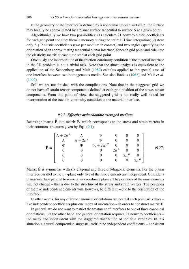
Trim: 247mm × 174mm Top: 14.762mm Gutter: 23.198mmCUUK2497-09 CUUK2497/Moczo ISBN: 978 1 107 02881 4 November 16, 2013 11:36
206 VS SG scheme for unbounded heterogeneous viscoelastic medium
If the geometry of the interface is defined by a nonplanar smooth surface S, the surfacemay locally be approximated by a planar surface tangential to surface S at a given point.
Algorithmically we have two possibilities: (1) calculate 21 nonzero elastic coefficientsfor each grid point and store them in memory during the entire FD time integration; (2) storeonly 2 + 2 elastic coefficients (two per medium in contact) and two angles (specifying theorientation of an approximating tangential planar interface) for each grid point and calculatethe elasticity matrix at each time step at each grid point.
Obviously, the incorporation of the traction-continuity condition at the material interfacein the 3D problem is not a trivial task. Note that the above analysis is equivalent to theapplication of the Schoenberg and Muir (1989) calculus applied to the special case ofone interface between two homogeneous media. See also Backus (1962) and Muir et al.(1992).
Still we are not finished with the complications. Note that in the staggered grid wedo not have all strain-tensor components defined at each grid position of the stress-tensorcomponents. From this point of view, the staggered grid is not really well suited forincorporation of the traction-continuity condition at the material interface.
9.2.3 Effective orthorhombic averaged medium
Rearrange matrix ¯E into matrix E, which corresponds to the stress and strain vectors intheir common structures given by Eqs. (9.1):
E =
⎡⎢⎢⎢⎢⎢⎢⎢⎣
�+ 2μA � � 0 0 0� �+ 2μA � 0 0 0� � (λ+ 2μ)H 0 0 00 0 0 2μA 0 00 0 0 0 2μH 00 0 0 0 0 2μH
⎤⎥⎥⎥⎥⎥⎥⎥⎦
(9.27)
Matrix E is symmetric with six diagonal and three off-diagonal elements. For the planarinterface parallel to the xy -plane only five of the nine elements are independent. Consider aplanar interface parallel to some other coordinate planes. The positions of the nine elementswill not change – this is due to the structure of the stress and strain vectors. The positionsof the five independent elements will, however, be different – due to the orientation of theinterface.
In other words, for any of three canonical orientations we need at each point six values –five independent coefficients plus one index of orientation – in order to construct matrix E.
In general, we do not want to restrict the treatment of interfaces to one of three canonicalorientations. On the other hand, the general orientation requires 21 nonzero coefficients –too many and inconsistent with the staggered distribution of the field variables. In thissituation a natural compromise suggests itself: nine independent coefficients – consistent
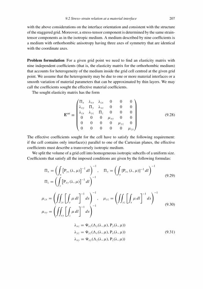
Trim: 247mm × 174mm Top: 14.762mm Gutter: 23.198mmCUUK2497-09 CUUK2497/Moczo ISBN: 978 1 107 02881 4 November 16, 2013 11:36
9.2 Stress–strain relation at a material interface 207
with the above considerations on the interface orientation and consistent with the structureof the staggered grid. Moreover, a stress-tensor component is determined by the same strain-tensor components as in the isotropic medium. A medium described by nine coefficients isa medium with orthorhombic anisotropy having three axes of symmetry that are identicalwith the coordinate axes.
Problem formulation For a given grid point we need to find an elasticity matrix withnine independent coefficients (that is, the elasticity matrix for the orthorhombic medium)that accounts for heterogeneity of the medium inside the grid cell centred at the given gridpoint. We assume that the heterogeneity may be due to one or more material interfaces or asmooth variation of material parameters that can be approximated by thin layers. We maycall the coefficients sought the effective material coefficients.
The sought elasticity matrix has the form
Eort ≡
⎛⎜⎜⎜⎜⎜⎜⎜⎝
x λxy λzx 0 0 0λxy y λyz 0 0 0λzx λyz z 0 0 00 0 0 μxy 0 00 0 0 0 μyz 00 0 0 0 0 μzx
⎞⎟⎟⎟⎟⎟⎟⎟⎠
(9.28)
The effective coefficients sought for the cell have to satisfy the following requirement:if the cell contains only interface(s) parallel to one of the Cartesian planes, the effectivecoefficients must describe a transversely isotropic medium.
We split the volume of a grid cell into homogeneous isotropic subcells of a uniform size.Coefficients that satisfy all the imposed conditions are given by the following formulas:
x =(∫
x
[Pyz (λ,μ)
]−1dl
)−1
, y =(∫
y
[Pxz (λ,μ)]−1 dl
)−1
z =(∫
z
[Pxy (λ,μ)
]−1dl
)−1 (9.29)
μzx =(∫∫
zx
[∫y
μ dl
]−1
ds
)−1
, μyz =(∫∫
yz
[∫x
μ dl
]−1
ds
)−1
μxy =(∫∫
xy
[∫z
μ dl
]−1
ds
)−1 (9.30)
λxz = �xz(�y(λ,μ),Py(λ,μ))
λyz = �yz(�x(λ,μ),Px(λ,μ))
λxy = �xy(�z(λ,μ),Pz(λ,μ))
(9.31)

Trim: 247mm × 174mm Top: 14.762mm Gutter: 23.198mmCUUK2497-09 CUUK2497/Moczo ISBN: 978 1 107 02881 4 November 16, 2013 11:36
208 VS SG scheme for unbounded heterogeneous viscoelastic medium
Here,
Pξζ (λ,μ) =[∫∫
ξζ
λ
λ+ 2μdS
]2 (∫∫ξζ
1
λ+ 2μdS
)−1
+∫∫
ξζ
(λ+ 2μ− λ2
λ+ 2μ
)dS
�ξζ (λ,μ) = Pξζ (λ,μ) − 2∫∫
ξζ
μ dS
�ξζ (a, b) =∫∫
ξζ
a
bdS
(∫∫ξζ
1
bdS
)−1
(9.32)
The auxiliary parameters a and b stand for an appropriate Pξ (λ,μ) and �ξ (λ,μ), respec-tively. The last two parameters are evaluated as
Pξ (λ,μ) =[∫ξ
λ
λ+ 2μdl
]2 (∫ξ
1
λ+ 2μdl
)−1
+∫ξ
(λ+ 2μ− λ2
λ+ 2μ
)dl
�ξ (λ,μ) = Pξ (λ,μ) − 2∫ξ
μ dl
(9.33)
Note that the double subscript ξ, ζ indicates averaging over the ξ, ζ -plane. The singlesubscript ξ indicates averaging along the ξ -axis.
The effective elastic coefficients (moduli) have to be determined at the grid positionsof the stress-tensor components – according to the structures of vectors �σ and �ε given byEqs. (9.1) and matrix Eort given by Eq. (9.28). All x, y, z and λxy, λyz, λzx have to bedetermined at the grid position that is shared by all the normal stress-tensor components.Coefficient μxy has to be determined at the grid position of σxy , μyz at the grid position ofσyz, and μzx at the grid position of σzx .
Finally, the stress–strain relation for the orthorhombic averaged medium can be writtenas
σxx = xεxx + λxyεyy + λzxεzzσyy = λxyεxx + yεyy + λyzεzzσzz = λzxεxx + λyzεyy + zεzzσxy = μxyεxy, σyz = μyzεyz, σzx = μzxεzx
(9.34)
9.2.4 Effective grid density
It was shown in the analysis of the 1D problem in Section 7.4 that the effective (average)density representing the welded interface is the arithmetic average of densities in thehalfspaces. In 3D, at each position of the particle-velocity component (or displacementcomponent) an effective grid density is determined as a volume arithmetic average ofdensity within a volume of the grid cell centred at the grid position. The averaging appliesto both smoothly and discontinuously heterogeneous media. The averages are evaluated by
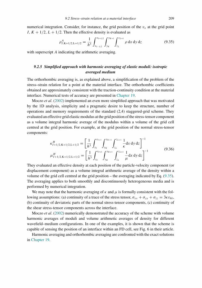
Trim: 247mm × 174mm Top: 14.762mm Gutter: 23.198mmCUUK2497-09 CUUK2497/Moczo ISBN: 978 1 107 02881 4 November 16, 2013 11:36
9.2 Stress–strain relation at a material interface 209
numerical integration. Consider, for instance, the grid position of the vx at the grid pointI,K + 1/2, L+ 1/2. Then the effective density is evaluated as
ρAI,K+1/2,L+1/2 = 1
h3
∫ xI+1/2
xI−1/2
∫ yK+1
yK
∫ zL+1
zL
ρ dx dy dz (9.35)
with superscript A indicating the arithmetic averaging.
9.2.5 Simplified approach with harmonic averaging of elastic moduli: isotropicaveraged medium
The orthorhombic averaging is, as explained above, a simplification of the problem of thestress–strain relation for a point at the material interface. The orthorhombic coefficientsobtained are approximately consistent with the traction-continuity condition at the materialinterface. Numerical tests of accuracy are presented in Chapter 19.
Moczo et al. (2002) implemented an even more simplified approach that was motivatedby the 1D analysis, simplicity and a pragmatic desire to keep the structure, number ofoperations and memory requirements of the standard (2,4) staggered-grid scheme. Theyevaluated an effective grid elastic modulus at the grid position of the stress-tensor componentas a volume integral harmonic average of the modulus within a volume of the grid cellcentred at the grid position. For example, at the grid position of the normal stress-tensorcomponents:
κHI+1/2,K+1/2,L+1/2 =[
1
h3
∫ xI+1
xI
∫ yK+1
yK
∫ zL+1
zL
1
κdx dy dz
]−1
μHI+1/2,K+1/2,L+1/2 =[
1
h3
∫ xI+1
xI
∫ yK+1
yK
∫ zL+1
zL
1
μdx dy dz
]−1 (9.36)
They evaluated an effective density at each position of the particle-velocity component (ordisplacement component) as a volume integral arithmetic average of the density within avolume of the grid cell centred at the grid position – the averaging indicated by Eq. (9.35).The averaging applies to both smoothly and discontinuously heterogeneous media and isperformed by numerical integration.
We may note that the harmonic averaging of κ and μ is formally consistent with the fol-lowing assumptions: (a) continuity of a trace of the stress tensor, σxx + σyy + σzz = 3κεkk ,(b) continuity of deviatoric parts of the normal stress-tensor components, (c) continuity ofthe shear stress-tensor components across the interface.
Moczo et al. (2002) numerically demonstrated the accuracy of the scheme with volumeharmonic averages of moduli and volume arithmetic averages of density for differentwavefield–medium configurations. In one of the examples, it is shown that the scheme iscapable of sensing the position of an interface within an FD cell, see Fig. 6 in their article.
Harmonic averaging and orthorhombic averaging are confronted with the exact solutionsin Chapter 19.
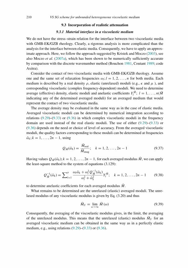
Trim: 247mm × 174mm Top: 14.762mm Gutter: 23.198mmCUUK2497-09 CUUK2497/Moczo ISBN: 978 1 107 02881 4 November 16, 2013 11:36
210 VS SG scheme for unbounded heterogeneous viscoelastic medium
9.3 Incorporation of realistic attenuation
9.3.1 Material interface in a viscoelastic medium
We do not have the stress–strain relation for the interface between two viscoelastic mediawith GMB-EK/GZB rheology. Clearly, a rigorous analysis is more complicated than theanalysis for the interface between elastic media. Consequently, we have to apply an approx-imate approach. Here, we follow the approach suggested by Kristek and Moczo (2003), seealso Moczo et al. (2007a), which has been shown to be numerically sufficiently accurateby comparison with the discrete wavenumber method (Bouchon 1981, Coutant 1989; codeAxitra).
Consider the contact of two viscoelastic media with GMB-EK/GZB rheology. Assumeone and the same set of relaxation frequencies ωl ; l = 1, 2, . . . , n for both media. Eachmedium is described by a real density ρ, elastic (unrelaxed) moduli (e.g., κ and μ ), andcorresponding viscoelastic (complex frequency-dependent) moduli. We need to determineaverage (effective) density, elastic moduli and anelastic coefficients Y Ml ; l = 1, . . . , n(Mindicating any of the determined averaged moduli) for an averaged medium that wouldrepresent the contact of two viscoelastic media.
The average density may be evaluated in the same way as in the case of elastic media.Averaged viscoelastic moduli can be determined by numerical integration according torelations (9.29)–(9.33) or (9.36) in which complex viscoelastic moduli in the frequencydomain are used instead of the real elastic moduli. The use of either (9.29)–(9.33) or(9.36) depends on the need or choice of level of accuracy. From the averaged viscoelasticmoduli, the quality factors corresponding to these moduli can be determined at frequenciesωk; k = 1, . . . , 2n− 1, using
QM (ωk) = Mreal
Mimag; k = 1, 2, . . . , 2n− 1 (9.37)
Having valuesQM (ωk); k = 1, 2, . . . , 2n− 1, for each averaged modulus M , we can applythe least-square method to the system of equations (3.129):
Q−1M
(ωk) =∑n
l=1
ωlωk + ω2l Q
−1M
(ωk)
ω2l + ω2
k
Y Ml ; k = 1, 2, . . . , 2n− 1 (9.38)
to determine anelastic coefficients for each averaged modulus M .What remains to be determined are the unrelaxed (elastic) averaged moduli. The unre-
laxed modulus of any viscoelastic modulus is given by Eq. (3.20) and thus
MU = limω→∞ M (ω) (9.39)
Consequently, the averaging of the viscoelastic modulus gives, in the limit, the averagingof the unrelaxed modulus. This means that the unrelaxed (elastic) modulus MU for anaveraged viscoelastic medium can be obtained in the same way as in a perfectly elasticmedium, e.g., using relations (9.29)–(9.33) or (9.36).

Trim: 247mm × 174mm Top: 14.762mm Gutter: 23.198mmCUUK2497-09 CUUK2497/Moczo ISBN: 978 1 107 02881 4 November 16, 2013 11:36
9.3 Incorporation of realistic attenuation 211
If we do not directly know the viscoelastic moduli κ(ω) and μ(ω) (or λ(ω) and μ(ω)) for each of the two media in contact but, instead, we know the measured or estimatedQα(ω) for the P wave and Qβ(ω) for the S wave, we have to proceed as follows. Weassume GMB-EK/GZB rheology for each medium as well as for the averaged medium.For each of the two media we first determine Yαl and Yβl using Eqs. (3.139) and then Y κland Yμl or Yλl and Yμl using Eqs. (3.140) or (3.142). Then, assuming known unrelaxedmoduli for each medium, we can determine the viscoelastic moduli using Eq. (3.126)for each modulus. Then we can proceed with numerical averaging of the moduli in thefrequency domain, determination of the corresponding quality factors, and determinationof the anelastic coefficients as described before.
9.3.2 Scheme for the anelastic functions for an isotropic averaged medium
In Section 7.8 we presented the FD scheme for the anelastic functions for a 1D smoothmedium. Here we obtain the scheme in 3D in an analogous way. Recall the constitutivelaw in the velocity–stress formulation for the viscoelastic continuum with GMB-EK/GZBrheology, Eqs. (3.136) and (3.137):
∂
∂tσij = κ ∂
∂tεkkδij + 2μ
(∂
∂tεij − 1
3
∂
∂tεkkδij
)−∑n
l=1
[Y κl κξ
kkl δij + 2Yμl μ
(ξijl − 1
3ξkkl δij
)] (9.40)
∂
∂tξijl (t) + ωlξ ijl (t) = ωl ∂
∂tεij (t), l = 1, . . . , n (9.41)
Except for the superscripts in the anelastic coefficients, κ and μ are the unrelaxed (elastic)moduli. Relation (9.40) can apply to either a smoothly heterogeneous viscoelastic mediumor isotropic averaged medium. For simplicity we do not use an overbar to distinguish theaveraged medium.
The anelastic functions and their temporal derivatives can be approximated with the2nd-order accuracy:
ξijl (tm−1/2)
.= 12
[ξijl (tm) + ξ ijl (tm−1)
], l = 1, . . . , n (9.42)
∂
∂tξijl (t)
∣∣∣∣m−1/2.= 1
�
[ξijl (tm) − ξ ijl (tm−1)
], l = 1, . . . , n (9.43)
Using approximations (9.42) and (9.43) in Eq. (9.41) we obtain a scheme for updating theanelastic functions:
ξijl (tm)
.= 2ωl�
2 + ωl�∂εij
∂t
∣∣∣∣m−1/2
+ 2 − ωl�2 + ωl�ξ
ijl (tm−1), l = 1, . . . , n (9.44)

Trim: 247mm × 174mm Top: 14.762mm Gutter: 23.198mmCUUK2497-09 CUUK2497/Moczo ISBN: 978 1 107 02881 4 November 16, 2013 11:36
212 VS SG scheme for unbounded heterogeneous viscoelastic medium
According to Eq. (9.42), both ξ ijl (tm) and ξ ijl (tm−1) have to be kept in memory for updatingξijl (tm−1/2). To avoid this, we can use approximation (9.42) in Eq. (9.44) to eliminateξijl (tm−1) (Kristek and Moczo 2003):
ξijl (tm−1/2)
.= − ωl�
2 − ωl�∂εij
∂t
∣∣∣∣m−1/2
+ 2
2 − ωl�ξijl (tm), l = 1, . . . , n (9.45)
Using Eq. (9.45) in Eq. (9.40) for time tm−1/2 we obtain
∂σij
∂t
∣∣∣∣m−1/2
= κ ∂εkk∂t
∣∣∣∣m−1/2
δij + 2μ
(∂εij
∂t
∣∣∣∣m−1/2
− 13
∂εkk
∂t
∣∣∣∣m−1/2
δij
)
−∑n
l=1
[Y κl ξ
kkl (tm)δij + 2Y μl
(ξijl (tm) − 1
3ξkkl (tm)δij
)] (9.46)
where
κ = κ (1 +∑nl=1G1lY
κl
), μ = μ (1 +∑n
l=1G1lYμl
)Y κl = G2lκY
κl , Y
μl = G2lμY
μl
G1l = ωl�2−ωl� , G2l = 2
2−ωl�
(9.47)
The derived relations mean that first we calculate ξ ijl (tm) using relation (9.44) and then weapply the obtained values in relation (9.46).
9.3.3 Scheme for anelastic functions for an orthorhombic averaged medium
Consider, for example, σxx for the elastic continuum given by the stress–strain relation(9.34):
σxx = xεxx + λxyεyy + λzxεzz (9.48)
In the velocity–stress formulation we need its temporal derivative:
∂σxx
∂t= x ∂εxx
∂t+ λxy ∂εyy
∂t+ λzx ∂εzz
∂t(9.49)
The corresponding stress–strain relation for the viscoelastic continuum with GMB-EK/GZBrheology is
∂σxx
∂t= x ∂εxx
∂t+ λxy ∂εyy
∂t+ λzx ∂εzz
∂t
−∑n
l=1
[Y xl xξ
xxl + Yλxyl λxyξyyl + Yλzxl λzxξ zzl
] (9.50)
The additional ordinary differential equations for the anelastic functions ξxxl , ξyyl and ξzzlsatisfy Eqs. (9.41). It is easy to derive the relation for ∂σxx
∂t
∣∣m−1/2and also for the tempo-
ral derivatives of the other stress-tensor components similar to (9.46) using a procedureanalogous to that explained in the previous subsection.

Trim: 247mm × 174mm Top: 14.762mm Gutter: 23.198mmCUUK2497-09 CUUK2497/Moczo ISBN: 978 1 107 02881 4 November 16, 2013 11:36
9.3 Incorporation of realistic attenuation 213
9.3.4 Coarse spatial distribution of anelastic functions
The GMB-EK/GZB rheology enables reasonably realistic modelling of attenuation. Itsincorporation, however, considerably increases the number of operations and variables/parameters. Therefore Zeng (1996), and independently Day (1998) and Day and Bradley(2001), introduced coarse spatial sampling of the anelastic functions and coefficients inorder to significantly reduce the increased memory requirements and also computationaltime. In Day’s (1998) approach, one anelastic function ξ ijl for one relaxation frequency ωlis distributed with a spatial period 2h. Then the number of relaxation frequencies is n = 8.Considering, for example, location of the stress-tensor component σzx at the eight verticesof a grid cube with edge h, only one of the eight anelastic functions ξzxl is assigned to eachone of the eight vertices (ξzx1 is assigned to one position, ξzx2 to another position, and soon). Then the total number of anelastic functions ξzxl ; l = 1, 2, . . . , 8 in the whole grid is12MX · 1
2MY · 12MZ · 8 = MX ·MY ·MZ, whereMX,MY andMZ are the numbers of
grid cells in the three Cartesian directions, respectively. Because there are six independentstrain-tensor components, the total number of all anelastic functions in the whole grid isMX ·MY ·MZ · 6. Since the anelastic coefficients YMl may be distributed in the samecoarse manner, the total number of anelastic coefficients in the grid isMX ·MY ·MZ · 9in the case of an orthorhombic averaged medium. In the case of harmonic averaging of themoduli, the number of anelastic coefficients is MX ·MY ·MZ · 5 in the staggered gridor MX ·MY ·MZ · 2 in the conventional grid. This means that the additional memoryfor a coarse distribution and eight relaxation frequencies is equivalent to the additionalmemory required by just one relaxation mechanism (that is, one relaxation frequency)without coarse sampling. Such a reduction of the memory requirements is significant.Graves and Day (2003) analyzed the stability and accuracy of the scheme with coarsespatial sampling and defined the effective modulus and quality factor necessary to achievesufficient accuracy, especially in the case of very lowQ.
In a structurally complex model there are material interfaces going through grid cellsin different orientations with respect to the coordinate system. In such a case and withthe originally suggested spatial sampling, it may happen that the medium from one sideof the material interface is characterized over one half of the whole considered frequencyrange while the medium from the other side of the interface is characterized over the otherhalf of the considered frequency range. This means that the behaviours of the two mediain contact are described in two disjunctive frequency sub-intervals. Consequently, the twomedia cannot physically interact.
The geometry of coarse spatial sampling shown by Day (1998) and Day and Bradley(2001) is only one of several possible distributions. Keeping the same spatial periodic-ity of the anelastic quantities, we can choose such a distribution in which division of agrid cell into two parts characterized in two disjunctive frequency sub-intervals is alwaysavoided. However, with any type of geometric distribution the best possible situation wouldbe, for example, characterization of one medium in contact using relaxation frequenciesω1, ω3, ω5, ω7 and characterization of the other medium in contact using ω2, ω4, ω6, ω8.

Trim: 247mm × 174mm Top: 14.762mm Gutter: 23.198mmCUUK2497-09 CUUK2497/Moczo ISBN: 978 1 107 02881 4 November 16, 2013 11:36
214 VS SG scheme for unbounded heterogeneous viscoelastic medium
1
1
2
2
3
3
4
4
4n =
/ 2h
/ 2h
Figure 9.1 Coarse spatial distribution of grid cells and anelastic functions. The number on a cell faceindicates the relaxation frequency of the anelastic functions localized in the cell. For example, gridcell 1 contains ξxx1 , ξ
yy1 , ξ
zz1 , ξ
xy1 , ξ
yz1 , ξ
zx1 . (Reproduced from Kristek and Moczo 2003)
This is much better than two disjunctive frequency sub-intervals, but still not sufficientlysatisfactory.
Summation in the anelastic parts of the stress–strain relation (9.40) or (9.46) includesanelastic functions and coefficients at all relaxation frequencies ωl ; l = 1, 2, . . . , n. Incoarse spatial sampling, however, at any one grid position we have an anelastic functiononly at one relaxation frequency. Still, it is possible to account for all the anelastic functionsand coefficients: the anelastic functions and coefficients from the neighbouring positionsare taken with properly weighting coefficients and averaged together at the grid point wherethe stress-tensor component is to be evaluated.
Such averaging is possible with the material-independent anelastic functions introducedby Kristek and Moczo (2003), see Subsection 3.3.10. This is because averaging of thematerial-independent anelastic functions does not introduce additional unjustified averagingof the material properties. Note that this would be the case with the original material-dependent anelastic functions introduced by Day and Minster (1984), Emmerich and Korn(1987), Carcione et al. (1988a,b) and Robertsson et al. (1994).
Kristek and Moczo (2003) also suggested an alternative coarse spatial distribution ofthe anelastic functions that requires only n = 4 relaxation frequencies, keeping the samememory requirements as in the approach by Day (1998) and Day and Bradley (2001). Thedistribution is shown in Fig. 9.1. Kristek and Moczo (2003) numerically demonstrated theaccuracy of their FD scheme with the material-independent anelastic functions and a newcoarse distribution of the anelastic functions by comparison with the discrete wavenumbermethod (Bouchon 1981, Coutant 1989; code Axitra).

Trim: 247mm × 174mm Top: 14.762mm Gutter: 23.198mmCUUK2497-09 CUUK2497/Moczo ISBN: 978 1 107 02881 4 November 16, 2013 11:36
9.3 Incorporation of realistic attenuation 215
9.3.5 VS SG (2,4) scheme for a heterogeneous viscoelastic medium
For brevity we show only the scheme for the x -component of the particle velocity, thexx -component of the stress tensor, and the xx anelastic function, that is, for vx , σxx , andξxxl . Schemes for the other components are analogous. Denote the discrete grid values ofthe particle velocity components vx, vy, vz by VX,V Y, VZ, respectively. Similarly denotethe stress-tensor components σxx, σxy, σzx by TXX,TXY,TZX. For other quantities we usethe same symbols as in the corresponding equations. The schemes for vx and σxx are then(compare with the 1D schemes (7.331)–(7.333))
VXm+1/2I,K+1/2,L+1/2 = VXm−1/2
I,K+1/2,L+1/2 + �
ρI,K+1/2,L+1/2f |mI,K+1/2,L+1/2
+ 1
ρI,K+1/2,L+1/2
�
h
[98
(TXXmI+1/2,K+1/2,L+1/2 − TXXmI−1/2,K+1/2,L+1/2
)− 1
24
(TXXmI+3/2,K+1/2,L+1/2 − TXXmI−3/2,K+1/2,L+1/2
)+ 9
8
(TXYmI,K+1,L+1/2 − TXYmI,K,L+1/2
)− 1
24
(TXYmI,K+2,L+1/2 − TXYmI,K−1,L+1/2
)+ 9
8
(TZXmI,K+1/2,L+1 − TZXmI,K+1/2,L
)− 1
24
(TZXmI,K+1/2,L+2 − TZXmI,K+1/2,L−1
)]
(9.51)
TXXmI+1/2,K+1/2,L+1/2
= TXXm−1I+1/2,K+1/2,L+1/2
+ �h
{MXXI+1/2,K+1/2,L+1/2
[98
(VXm−1/2
I+1,K+1/2,L+1/2 − VXm−1/2I,K+1/2,L+1/2
)− 1
24
(VXm−1/2
I+2,K+1/2,L+1/2 − VXm−1/2I−1,K+1/2,L+1/2
)]+ MXYI+1/2,K+1/2,L+1/2
[98
(V Y
m−1/2I+1/2,K+1,L+1/2 − V Ym−1/2
I+1/2,K,L+1/2
)− 1
24
(V Y
m−1/2I+1/2,K+2,L+1/2 − V Ym−1/2
I+1/2,K−1,L+1/2
)]+ MZXI+1/2,K+1/2,L+1/2
[98
(VZ
m−1/2I+1/2,K+1/2,L+1 − VZm−1/2
I+1/2,K+1/2,L
)− 1
24
(VZ
m−1/2I+1/2,K+1/2,L+2 − VZm−1/2
I+1/2,K+1/2,L−1
)]}−�
∑n
l=1
(YMXXl;I+1/2,K+1/2,L+1/2 ξ
xx;ml;I+1/2,K+1/2,L+1/2
+ YMXYl;I+1/2,K+1/2,L+1/2 ξ
yy;ml;I+1/2,K+1/2,L+1/2 + YMXZ
l;I+1/2,K+1/2,L+1/2 ξzz;ml;I+1/2,K+1/2,L+1/2
)
(9.52)
The scheme for ξxxl corresponding to Eq. (9.44) is
ξxx;ml;I+1/2,K+1/2,L+1/2 = 2 − ωl�
2 + ωl� ξxx;m−1l;I+1/2,K+1/2,L+1/2
+ 2ωl�
2 + ωl�1
h
[98
(VXm−1/2
I+1,K+1/2,L+1/2 − VXm−1/2I,K+1/2,L+1/2
)− 1
24
(VXm−1/2
I+2,K+1/2,L+1/2 − VXm−1/2I−1,K+1/2,L+1/2
)](9.53)
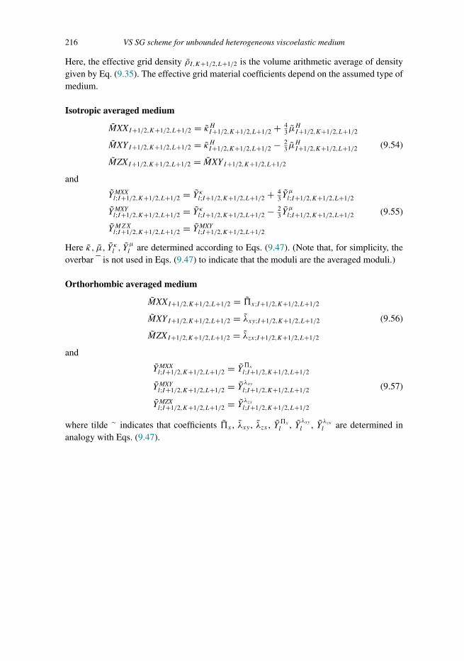
Trim: 247mm × 174mm Top: 14.762mm Gutter: 23.198mmCUUK2497-09 CUUK2497/Moczo ISBN: 978 1 107 02881 4 November 16, 2013 11:36
216 VS SG scheme for unbounded heterogeneous viscoelastic medium
Here, the effective grid density ρI,K+1/2,L+1/2 is the volume arithmetic average of densitygiven by Eq. (9.35). The effective grid material coefficients depend on the assumed type ofmedium.
Isotropic averaged medium
MXXI+1/2,K+1/2,L+1/2 = κHI+1/2,K+1/2,L+1/2 + 43 μHI+1/2,K+1/2,L+1/2
MXYI+1/2,K+1/2,L+1/2 = κHI+1/2,K+1/2,L+1/2 − 23 μHI+1/2,K+1/2,L+1/2
MZXI+1/2,K+1/2,L+1/2 = MXYI+1/2,K+1/2,L+1/2
(9.54)
and
YMXXl;I+1/2,K+1/2,L+1/2 = Y κl;I+1/2,K+1/2,L+1/2 + 4
3 Yμl;I+1/2,K+1/2,L+1/2
YMXYl;I+1/2,K+1/2,L+1/2 = Y κl;I+1/2,K+1/2,L+1/2 − 2
3 Yμl;I+1/2,K+1/2,L+1/2
Y MZXl;I+1/2,K+1/2,L+1/2 = YMXYl;I+1/2,K+1/2,L+1/2
(9.55)
Here κ, μ, Y κl , Yμl are determined according to Eqs. (9.47). (Note that, for simplicity, the
overbar ¯ is not used in Eqs. (9.47) to indicate that the moduli are the averaged moduli.)
Orthorhombic averaged medium
MXXI+1/2,K+1/2,L+1/2 = x;I+1/2,K+1/2,L+1/2
MXYI+1/2,K+1/2,L+1/2 = λxy;I+1/2,K+1/2,L+1/2
MZXI+1/2,K+1/2,L+1/2 = λzx;I+1/2,K+1/2,L+1/2
(9.56)
and
YMXXl;I+1/2,K+1/2,L+1/2 = Y xl;I+1/2,K+1/2,L+1/2
YMXYl;I+1/2,K+1/2,L+1/2 = Y λxyl;I+1/2,K+1/2,L+1/2
YMZXl;I+1/2,K+1/2,L+1/2 = Y λzxl;I+1/2,K+1/2,L+1/2
(9.57)
where tilde � indicates that coefficients x , λxy , λzx , Y xl , Y
λxyl , Y λzxl are determined in
analogy with Eqs. (9.47).

Trim: 247mm × 174mm Top: 14.762mm Gutter: 23.198mmCUUK2497-10 CUUK2497/Moczo ISBN: 978 1 107 02881 4 November 19, 2013 17:27
10
Schemes for a free surface
The free surface was briefly introduced in Subsection 2.5.1 and Section 7.5. The 1D FDschemes for modelling the free surface based on the stress-imaging technique and adjustedFD approximations were presented in Subsections 7.5.1 and 7.5.2, respectively. Recall theboundary conditions. Considering a free surface S with normal vector �n and traction vector�T (�n), the traction-free condition at S, �T (�n) = 0, implies
σijnj = 0 (10.1)
10.1 Planar free surface
If surface S is planar and perpendicular to the z-axis, �n = (0, 0,−1) and Eq. (10.1) implies
σiz = 0; i ∈ {x, y, z} (10.2)
It is significantly simpler to implement the traction-free condition (10.2) than condition(10.1) in an FD scheme. This is why FD modelling of a planar free surface is reasonablyfeasible whereas FD modelling of free-surface topography still poses a major challenge.
As mentioned in Chapter 7, we have two principal possibilities for calculating particlevelocity at and near the free surface. The first approach: apply the scheme for the interiorgrid points assuming virtual values of stress, particle velocity and material parametersoutside the medium. The second approach: apply one-sided schemes that do not need anyvirtual values outside the medium. The advantage of the first approach is the use of oneand the same scheme at any grid point. Its disadvantage is the need to define virtual valuesreasonably outside the medium. The disadvantage of the second approach is the use ofdifferent schemes for different grid positions at and near the free surface.
The first approach leads to the so-called vacuum formalism, medium taper or imagingmethod. The vacuum formalism applies zero moduli above the free surface. The vacuum for-malism may yield a good level of accuracy in the conventional-grid displacement schemesfor low values of the P-wave to S-wave speed ratio as shown by Zahradnık and Priolo (1995)in 2D and Moczo et al. (1999) in 3D, for example. Graves (1996) and other authors didnot find the vacuum formalism satisfactory in staggered-grid modelling. A density taperwas used by Frankel and Leith (1992) in their displacement conventional-grid scheme.
217

Trim: 247mm × 174mm Top: 14.762mm Gutter: 23.198mmCUUK2497-10 CUUK2497/Moczo ISBN: 978 1 107 02881 4 November 19, 2013 17:27
218 Schemes for a free surface
Levander (1988) suggested using virtual values of the stress-tensor components above thefree surface and applying the antisymmetry condition for the stress-tensor componentsabout the free surface. He applied the approach to his 2D (2,4) VS SG scheme. Levander’stechnique may reasonably be called the stress-imaging technique. Rodrigues (1993) devel-oped a 3D eighth-order staggered-grid displacement–stress scheme and used stress imagingwith the normal stress-tensor components at the free surface. He found that it is necessary totake 10 to 15 grid points per shortest wavelength to avoid significant numerical dispersion.Therefore, he combined the stress-imaging technique with a vertically refined grid nearthe free surface and achieved good accuracy. Graves (1996) applied stress imaging withthe normal stress-tensor components at the free surface in his 3D (2,4) VS SG modelling.Graves gave a clear explanation of the treatment of the stress-tensor and particle-velocitycomponents at and above the free surface. Robertsson (1996) summarized three possibili-ties for treating the particle-velocity values at grid positions above the free surface requiredby the (2,4) VS SG scheme. (1) The values are calculated using the 2nd-order approxima-tions to the boundary condition and imaged stress tensor components (e.g., Levander 1988,Graves 1996, Kristek et al. 2002). (2) The values are mirrored as symmetric values withrespect to the free surface (e.g., Crase 1990, Rodrigues and Mora 1993). (3) Robertsson(1996) assumed zero values. Gottschammer and Olsen (2001) compared a formulationwith horizontal particle-velocity components (and normal stress-tensor components) at thefree surface with a formulation with the vertical particle-velocity component at the freesurface in the 3D (2,4) VS SG scheme in a homogeneous halfspace. They concluded with arecommendation to use the formulation with the vertical particle-velocity component at thefree surface and to apply averaging across the free surface in order to obtain values of thehorizontal components at the free surface. The comparison was performed for the commonspatial sampling that was shown by Kristek et al. (2002) to be insufficient.
Applying the second approach, Kristek et al. (2002) and Moczo et al. (2004a) developeda 4th-order scheme with adjusted FD approximations and demonstrated its better accuracycompared to stress imaging.
10.1.1 Stress imaging in the (2,4) VS SG scheme
As mentioned before, in the staggered grid there are two obvious options for localizingthe planar free surface. (a) The free surface coincides with the grid plane with positionsvx, vy, σxx, σyy, σzz, σxy . Because the horizontal components of the particle velocity are atthe free surface we may call this option, for brevity, the H formulation or configuration. (b)The free surface coincides with the grid plane with positions vz, σyz, σzx . We indicate thisformulation by letter W.
The antisymmetry
σzx(−z) = −σzx(z), σyz(−z) = −σyz(z), σzz(−z) = −σzz(z) (10.3)
ensures the free-surface condition (10.2).
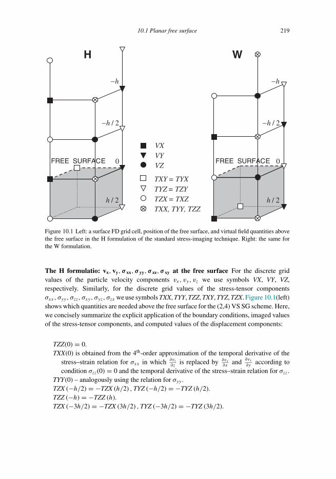
Trim: 247mm × 174mm Top: 14.762mm Gutter: 23.198mmCUUK2497-10 CUUK2497/Moczo ISBN: 978 1 107 02881 4 November 19, 2013 17:27
10.1 Planar free surface 219
VXVYVZ
FREE SURFACE FREE SURFACE
H W
TXY = TYXTYZ = TZYTZX = TXZTXX, TYY, TZZ
/ 2h−
h−
0
/ 2h
/ 2h−
h−
0
/ 2h
Figure 10.1 Left: a surface FD grid cell, position of the free surface, and virtual field quantities abovethe free surface in the H formulation of the standard stress-imaging technique. Right: the same forthe W formulation.
The H formulatio: vx, vy, σ xx, σ yy, σ zz, σ xy at the free surface For the discrete gridvalues of the particle velocity components vx, vy, vz we use symbols VX, VY, VZ,respectively. Similarly, for the discrete grid values of the stress-tensor componentsσxx, σyy, σzz, σxy, σyz, σzx we use symbols TXX, TYY, TZZ, TXY, TYZ, TZX. Figure 10.1(left)shows which quantities are needed above the free surface for the (2,4) VS SG scheme. Here,we concisely summarize the explicit application of the boundary conditions, imaged valuesof the stress-tensor components, and computed values of the displacement components:
TZZ(0) = 0.TXX(0) is obtained from the 4th-order approximation of the temporal derivative of the
stress–strain relation for σxx in which ∂vz∂z
is replaced by ∂vx∂x
and ∂vy∂y
according tocondition σzz(0) = 0 and the temporal derivative of the stress–strain relation for σzz.
TYY(0) – analogously using the relation for σyy .TZX (−h/2) = −TZX (h/2) ,TYZ (−h/2) = −TYZ (h/2).TZZ (−h) = −TZZ (h).TZX (−3h/2) = −TZX (3h/2) ,TYZ (−3h/2) = −TYZ (3h/2).

Trim: 247mm × 174mm Top: 14.762mm Gutter: 23.198mmCUUK2497-10 CUUK2497/Moczo ISBN: 978 1 107 02881 4 November 19, 2013 17:27
220 Schemes for a free surface
VX(0) is obtained from the 4th-order approximation of the equation for vx in which ∂σzx∂z
is also obtained using imaged σzx values.VY(0) – analogously using vy ,
∂σyz∂z
and σyz.VZ (−h/2) is obtained from the 2nd-order approximation of condition σzz(0) = 0 and
the temporal derivative of the stress–strain relation for σzz.VX (−h) is obtained from the 2nd-order approximation of σzx (−h/2) = −σzx (h/2) and
the temporal derivative of the stress–strain relation for σzx .VY (−h) – analogously using σyz.
The treatment of the other quantities is the same as in the case of the interior grid points.
The W formulatio: vz, σ yz, σ zx at the free surface Figure 10.1(right) shows which quan-tities are needed above the free surface for the (2,4) VS SG scheme. The formulation maybe summarized as follows:
TZX(0) = 0,TYZ(0) = 0.TZZ(−h/2) = −TZZ(h/2).TZX(−h) = −TZX(h),TYZ(−h) = −TYZ(h).TZZ(−3h/2) = −TZZ(3h/2).VZ(0) is obtained from the 4th-order approximation of the equation for vz in which ∂σzz
∂z
is also obtained using imaged σzz values.VX(−h/2) is obtained from the 2nd-order approximation of the condition σzx(0) = 0 and
the temporal derivative of the stress–strain relation for σzx .VY(−h/2) – analogously using σyz(0) = 0 and σyz.VZ(−h) is obtained from the 2nd-order approximation of σzz(−h/2) = −σzz(h/2) and
the temporal derivative of the stress–strain relation for σzz.
Treatment of the other quantities is the same as in the case of the interior grid points.
Comparison of the H and W formulations Although the principle is the same for bothformulations, there are differences indicating possibly different numerical results. Theimplementation differences are summarized in Table 10.1.
Kristek et al. (2002) performed extensive numerical tests of both formulations againstthe discrete-wavenumber (DWN) method (Bouchon 1981, Coutant 1989; code Axitra).The numerical investigations showed that the W formulation is a little more accu-rate (indicated by the numbers in Table 10.1). However, the difference may be con-sidered negligible with respect to the fact that both formulations need at least twiceas many grid spacings per minimum wavelength compared to the scheme for the inte-rior grid points if Rayleigh surface waves are to be propagated without significant griddispersion.
Rodrigues (1993) used a grid that was refined only in the vertical direction and only downto a necessary depth in his eighth-order velocity–stress scheme. In his implementation, the
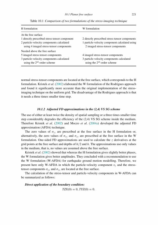
Trim: 247mm × 174mm Top: 14.762mm Gutter: 23.198mmCUUK2497-10 CUUK2497/Moczo ISBN: 978 1 107 02881 4 November 19, 2013 17:27
10.1 Planar free surface 221
Table 10.1 Comparison of two formulations of the stress-imaging technique
H formulation W formulation
At the free surface1 directly prescribed stress-tensor component2 particle-velocity components calculated
using 4 imaged stress-tensor components
2 directly prescribed stress-tensor components1 particle-velocity component calculated using
2 imaged stress-tensor components
Needed above the free surface5 imaged stress-tensor components3 particle-velocity components calculated
using the 2nd-order scheme
4 imaged stress-tensor components3 particle-velocity components calculated
using the 2nd-order scheme
normal stress-tensor components are located at the free surface, which corresponds to the Hformulation. Kristek et al. (2002) elaborated the W formulation of the Rodrigues approachand found it significantly more accurate than the original implementation of the stress-imaging technique on the uniform grid. The disadvantage of the Rodrigues approach is thatit needs a three times smaller time step.
10.1.2 Adjusted FD approximations in the (2,4) VS SG scheme
The use of either at least twice the density of spatial sampling or a three times smaller timestep considerably degrades the efficiency of the (2,4) VS SG scheme inside the medium.Therefore Kristek et al. (2002) and Moczo et al. (2004a) developed the adjusted FDapproximation (AFDA) technique.
The zero values of σzz are prescribed at the free surface in the H formulation or,alternatively, the zero values of σyz and σzx are prescribed at the free surface in the Wformulation. One-sided FD approximations are used to calculate the z derivatives at thegrid points at the free surface and depths of h/2 and h. The approximations use only valuesin the medium, that is, no values are assumed above the free surface.
Kristek et al. (2002) showed that whereas the H formulation gives slightly better phases,the W formulation gives better amplitudes. They concluded with a recommendation to usethe W formulation (W-AFDA) for earthquake ground motion modelling. Therefore, wepresent here only W-AFDA in which the particle-velocity component vz and the stress-tensor components σzx and σyz are located at the free surface.
The calculation of the stress-tensor and particle-velocity components in W-AFDA canbe summarized as follows:
Direct application of the boundary condition:
TZX(0) = 0,TYZ(0) = 0.

Trim: 247mm × 174mm Top: 14.762mm Gutter: 23.198mmCUUK2497-10 CUUK2497/Moczo ISBN: 978 1 107 02881 4 November 19, 2013 17:27
222 Schemes for a free surface
4th-order approximations of the z derivative:
The following 4th-order approximations of the 1st derivative with respect to the z -coordinateare used in calculations of the stress-tensor and particle-velocity vector components:
∂�
∂z(z0) = 1
h
[− 352105� (z0) + 35
8 �(z0 + 1
2h)− 35
24�(z0 + 3
2h)
+ 2140�
(z0 + 5
2h)− 5
56�(z0 + 7
2h)]+O(h4)
(10.4)
∂�
∂z(z0) = 1
h
[− 1112�
(z0 − 1
2h)+ 17
24�(z0 + 1
2h)+ 3
8�(z0 + 3
2h)
− 524�
(z0 + 5
2h)+ 1
24�(z0 + 7
2h)]+O(h4)
(10.5)
∂�
∂z(z0) = 1
h
[− 112h� (z0 − h) − 577
528�(z0 − 1
2h)+ 201
176�(z0 + 1
2h)
− 9176�
(z0 + 3
2h)+ 1
528�(z0 + 5
2h)]+O(h4)
(10.6)
∂�
∂z(z0) = 1
h
[16
105� (z0 − h) − 3124�
(z0 − 1
2h)+ 29
24�(z0 + 1
2h)
− 340�
(z0 + 3
2h)+ 1
168�(z0 + 5
2h)]+O(h4)
(10.7)
Depending on the particular configuration,�may stand for particle-velocity or stress-tensorcomponents and z0 for 0, h/2 or h.
(a) Calculation of the stress-tensor components:
TXX(h�2) is obtained from the 4th-order approximation of the temporal derivative ofthe stress–strain relation for σxx ;
∂vz∂z
is approximated using Eq. (10.5).TYY(h�2) and TZZ(h/2) – analogous to TXX(h/2).TZX(h) is obtained from the 4th-order approximation of the temporal derivative of the
stress–strain relation for σzx ;∂vx∂z
is approximated using Eq. (10.6) in which ∂vx∂z
(0)
is replaced by ∂vz∂x
(0) due to condition σzx(0) = 0.TYZ(h) is obtained from the 4th-order approximation of the temporal derivative of the
stress–strain relation for σyz;∂vy∂z
is approximated using Eq. (10.6) in which ∂vy∂z
(0)
is replaced by ∂vz∂y
(0) due to condition σyz(0) = 0.
(b) Calculation of the particle-velocity components:
VZ(0) is obtained from the 4th-order approximation of the equation for vz;∂σzz∂z
isapproximated using Eq. (10.4) in which condition σzz(0) = 0 is used.
VX(h�2) is obtained from the 4th-order approximation of the equation for vx ;∂σzx∂z
isapproximated using Eq. (10.5).
VY(h�2) is obtained from the 4th-order approximation of the equation for vy ;∂σyz∂z
isapproximated using Eq. (10.5).
VZ(h�2) is obtained from the 4th-order approximation of the equation for vz;∂σzz∂z
isapproximated using Eq. (10.7) in which condition σzz(0) = 0 is used.

Trim: 247mm × 174mm Top: 14.762mm Gutter: 23.198mmCUUK2497-10 CUUK2497/Moczo ISBN: 978 1 107 02881 4 November 19, 2013 17:27
10.2 Free-surface topography 223
The corresponding effective grid material parameters are evaluated as integral averagesin the half grid-cell volumes; that is, the upper half of the volume located above the freesurface is not taken into account. For example,
ρAI+1/2,K+1/2,0 = 2
h3
∫ xI+1
xI
∫ yK+1
yK
∫ z1/2
z0
ρ dx dy dz (10.8)
10.2 Free-surface topography
Implementation of the traction-free condition at a nonplanar surface has been one of themost difficult tasks and persisting challenges in FD modelling of seismic wave propagationand earthquake motion. The nonplanar free surface was addressed in the pioneering yearsof FDM in seismology by, e.g., Alterman and Rotenberg (1969), Alterman and Loewenthal(1970), Boore (1972a,b), Loewenthal and Alterman (1972), Munasinghe and Farnell (1973),Alterman and Nathaniel (1975), Ilan et al. (1975), Ilan and Loewenthal (1976). All theauthors treated simple types of free-surface topography: e.g., one-quarter and three-quarterplanes (90◦ and 270◦ vertices), a (0–180)◦ wedge, a vertical step discontinuity. Ilan (1977)and Jih et al. (1988) addressed an arbitrary polygonal free surface. The developed techniqueswere for 2D problems: SH (anti-plane horizontally polarized S waves in the vertical plane)or P-SV (in-plane P and vertically polarized S waves in the vertical plane). Whereasapparently the SH modelling did not pose a problem, the P-SV modelling faced problemswith stability and limitations in terms of the free-surface geometry and the P-wave to S-wave speed ratio (VP /VS) due to conversion between the P and S waves. Mainly due tothe problem in the case of large VP /VS , further development was mostly related to thevelocity–stress or displacement–stress staggered-grid schemes, e.g., Hestholm and Ruud(1994, 1998, 2002), Pitarka and Irikura (1996), Robertsson (1996), Ohminato and Chouet(1997), Robertsson and Holliger (1997), Hestholm (1999), Hestholm et al. (1999), Hayashiet al. (2001).
A particular implementation of the traction-free condition at a nonplanar surface verymuch depends on the medium (e.g., elastic, viscoelastic with realistic attenuation), formu-lation of the equation of motion and stress–strain relation (e.g., strong-form displacement,displacement–stress or velocity–stress), grid geometry (e.g., Cartesian, curvilinear), gridtype (conventional, collocated, staggered, partly staggered), free-surface geometry (e.g.,staircase, smooth), and dimensionality (2D, 3D). The mentioned aspects are reflected ina large variety of developed approaches and techniques. Correspondingly, we could fol-low alternative hierarchies in order to structure an overview of the recent approaches andtechniques.
In the numerical modelling of seismic wave propagation and earthquake motion insurface local sedimentary structures it is important that the technique is at least stable andsufficiently accurate in sediments with the P-wave to S-wave speed ratio equal to 5 andeven larger. We say ‘at least’ because these requirements should still go together withcomputational efficiency. Considering the three criteria (stability, VP /VS , efficiency), there
Trim: 247mm × 174mm Top: 14.762mm Gutter: 23.198mmCUUK2497-10 CUUK2497/Moczo ISBN: 978 1 107 02881 4 November 19, 2013 17:27
224 Schemes for a free surface
is still a need for further elaboration and development – despite significant progress inrecent years.
Note that in the case of large VP /VS it is not just about the stability. It is also about theaccuracy (see Section 8.3).
Here we restrict our discussion to a brief and simplified overview and point out therecent articles that we consider the most relevant.
We may recognize three basic strategies for treating a nonplanar free surface in FDmodelling of seismic wave propagation and earthquake motion:
– FD schemes on Cartesian grids,– FD schemes on curvilinear (conforming or boundary-conforming) grids,– hybrid schemes combining an FD scheme with a method in which the implementation
of the traction-free condition is considerably easier than in the FDM.
FD schemes on Cartesian grids Apparently, the easiest approach is based on using astaircase approximation of the true surface. Examples of the approach are the techniquesdeveloped by Pitarka and Irikura (1996), Robertsson (1996), Ohminato and Chouet (1997),Robertsson and Holliger (1997), Hayashi et al. (2001). We may also mention the schemesby Oprsal and Zahradnık (1999) and Perez-Ruiz et al. (2005) but with a comment on theirprincipal limitation for the lowest values of VP /VS .
Muir et al. (1992) demonstrated noticeable artificial diffraction generated at the grid-related steps of the internal material interfaces. Clearly, the steps of the staircase free surfacecan produce even stronger artificial diffraction. Artificial diffraction may be masked inthe complex wavefield, which can also include true physical diffraction. Artificial step-related diffraction is considerably more visible on the differential seismograms. Artificialdiffraction may be reduced within a limited frequency range by using relatively smallspatial grid spacing. Numerical experience shows that with a staircase free surface it isnecessary to apply a considerably finer grid compared to the grid that would be sufficientfor the major part of the computational domain. Spatial oversampling of the wavefield canbe circumvented by grid refinement in the vicinity of the free surface (Robertsson andHolliger 1997, Hayashi et al. 2001). In any case, artificial diffraction cannot be removed, itcan only be reduced.
The problems with step-related artificial diffraction can be avoided using the immersed-interface (or embedded-boundary) approach, e.g., Kreiss and Petersson (2006), Lombardet al. (2008). Kreiss and Petersson considered the scalar 2nd-order wave equation withoutattenuation in 2D. Lombard and his colleagues also treated the 2D elastic problem but forthe 1st-order hyperbolic system in the velocity–stress formulation, which is considerablymore relevant for media with large VP /VS .
Lombard et al. (2008) considered the velocity–stress formulation on the collocated gridin which all particle-velocity and stress-tensor components share the same grid position(Lombard et al. used the term ‘single-grid scheme’). They formulated the task as follows:treat the smooth arbitrarily shaped boundaries as simply as the straight boundaries; make the

Trim: 247mm × 174mm Top: 14.762mm Gutter: 23.198mmCUUK2497-10 CUUK2497/Moczo ISBN: 978 1 107 02881 4 November 19, 2013 17:27
10.2 Free-surface topography 225
accuracy independent of the boundary position in the grid; maintain stability for long runs.They showed that the requirements can be met by applying an explicit approach involvingfictitious values of the solution in the vacuum. The calculation of the fictitious valuesis based on the boundary conditions and compatibility conditions satisfied by successivespatial derivatives of the solution, up to a given order depending on the spatial accuracy ofthe integration scheme. The traction-free conditions can be designed with arbitrary orderof accuracy without numerical instabilities. Ten grid points per minimum S wavelengthyields highly accurate results up to a propagation distance of 50 wavelengths. A logicalbut noticeable feature of the method is its capability of sub-cell resolution. Lombard et al.pointed out the possibility of instabilities in the case using a staggered grid and long-timeintegration.
The immersed-interface method needs further elaboration in order to include hetero-geneity of the medium, realistic attenuation and extension to 3D.
FD schemes on the curvilinear grids Curvilinear grids can align with the surface topog-raphy and naturally avoid artificial step-related diffraction. This idea attracted Hestholmand Ruud (1994, 1998, 2002), Hestholm (1999, 2003), Hestholm et al. (1999), Ruud andHestholm (2001), Zhang and Chen (2006), Appelo and Petersson (2009), Tarrass et al.(2011), Lan and Zhang (2011), Zhang et al. (2012) and other researchers in their effortsto implement free-surface topography in seismic modelling. Appelo and Petersson (2009)considered a 2D displacement formulation (2nd-order hyperbolic equations) in a perfectlyelastic medium. Lan and Zhang (2011) extended the approach by Appelo and Peters-son to the 3D problem in a perfectly elastic transversally isotropic medium. Other authorsconsidered the velocity–stress formulation. Hestholm and Ruud (2002) presented an imple-mentation of the free-surface condition at a nonplanar surface for a viscoelastic medium inthe 3D velocity–stress scheme on a staggered grid.
An interesting and innovative approach was presented by Zhang and Chen (2006) for 2Dand by Zhang et al. (2012) for 3D free-surface topography. They used the velocity–stressformulation on the collocated grid. This is an important aspect for applying the traction-freecondition. The authors transform the irregular surface in physical space into a ‘flat’ surfacein computational space using a boundary-conforming grid. The grid is a general curvilineargrid (not the vertical stretching grid as in previous approaches by other authors). Thefree-surface conditions are implemented at this ‘flat’ surface by traction imaging. Tractionimaging is logical since in the case of a nonplanar surface no single stress-tensor componentis zero at the free surface. They re-write the velocity–stress equations as velocity–stress–traction equations (Eqs. 39–41 in their article) for the curvilinear grid, set the tractionto zero at the surface and apply antisymmetric imaging of the traction components withrespect to the free surface. In the velocity–stress–traction equations, derivatives with respectto the coordinate perpendicular to the free surface in computational space involve onlytractions normal to the free surface – not the stress components. This is what the authorsconsider to be the main reason for the stability and accuracy of their modelling of the freesurface.
Trim: 247mm × 174mm Top: 14.762mm Gutter: 23.198mmCUUK2497-10 CUUK2497/Moczo ISBN: 978 1 107 02881 4 November 19, 2013 17:27
226 Schemes for a free surface
Zhang et al. (2012) avoided the odd–even decoupling oscillations associated with centredFD approximations on the collocated grid: they applied the optimized DRP MacCormackscheme, which alternately uses forward and backward difference operators in the Runge–Kutta time stepping method (see the 1D scheme in Subsection 7.3.6). The scheme is4th-order accurate in dispersion error. However, as pointed out by the authors, their tractionimaging at a nonplanar free surface is not restricted to the particular FD scheme theyused. Zhang et al. (2012) presented a numerical test for smooth 3D topography – theGaussian-shaped hill.
Although numerical tests for an unbounded medium with large VP /VS confirmed thevery good level of accuracy of the scheme (testing within the EuroseisTest Verification andValidation Project, CEA France), it is still desirable to test the accuracy with respect toVP /VS in the presence of the nonplanar free surface. The FD scheme developed by Zhanget al. (2012) should also be generalized for a viscoelastic medium with realistic attenuation.
Hybrid schemes Implementation of the traction-free condition is natural (though not nec-essarily more accurate) in the FEM. Moczo et al. (1997) combined a 2nd-order conventionalFD scheme with a 2nd-order FEM for 2D viscoelastic P-SV modelling of seismic motionin near-surface sedimentary/topographic structures. Galis et al. (2008) developed a hybridnumerical method for a 3D viscoelastic heterogeneous medium with a nonplanar free sur-face. The method is based on a combination of the (2,4) VS SG FD scheme, coveringa major part of the computational domain, with the (2,2) FEM, which can be applied toone or several relatively small subdomains. The FD and FE parts causally communicateat each time level in the FD–FE transition zone consisting of the FE Dirichlet boundary,FD–FE averaging zone and FD Dirichlet zone. The FE part can include the nonplanar freesurface and/or a dynamically rupturing fault. The (2,2) FE method is limited in its accuracyfor large VP /VS (see Moczo et al. 2010, 2011). Therefore, if the FE part were to includesediments with large VP /VS , the FE mesh should be sufficiently fine.
A possible hybrid combination of the FDM with other methods (e.g., meshless movingleast-square method) might be explored.

Trim: 247mm × 174mm Top: 14.762mm Gutter: 23.198mmCUUK2497-11 CUUK2497/Moczo ISBN: 978 1 107 02881 4 November 16, 2013 14:14
11
Discontinuous spatial grid
11.1 Overview of approaches
The main advantage of a uniform grid is the algorithmical simplicity of the FD scheme.The main disadvantage of a uniform grid covering a strongly heterogeneous medium isthe relatively large number of grid points and consequently the large number of algebraicoperations. Typically, wave speeds in surface sediment structures are smaller than wavespeeds beneath sediments, especially in a rock basement. If the minimum wave speed in theupper part of a computational model is smaller than that in the lower part of the model, itmay be advantageous to use a combination of a finer grid (the grid spacing h) and a coarsergrid (the grid spacingH > h). The finer grid may cover the upper part whereas the coarser,the lower part of the model. The total number of grid points in such a discontinuous spatialgrid can be significantly smaller than that in a uniform grid. Therefore, numerical andespecially FD modellers have made numerous efforts to implement discontinuous grids.
Before we introduce and explain the discontinuous grids, let us mention a simplerapproach to reduce the number of grid points. Boore (1970) was the first to use a rectangulargrid with varying size of grid spacings to model Love wave propagation. Mikumo andMiyatake (1987) applied varying grid spacing in the 3D case in a homogeneous medium.Moczo (1989) applied a grid with varying spacing to the 2D SH problem in a laterallyheterogeneous medium. Pitarka (1999) developed 4th-order approximations of the 1st spatialderivative on the staggered grid with varying grid spacing, assuming simple functionaldependence of a field variable on the spatial coordinate. His 3D velocity–stress schemeassumes variations of the grid spacings in all three coordinate directions. Grids of varyingspacing do not reach the efficiency of discontinuous grids. Our limited numerical experienceindicates a possible sensitivity of the simulated wavefield to variation in the size of the gridspacing, e.g., in the case of strong surface waves.
Jastram and Behle (1992) introduced a discontinuous grid with an arbitrary integer ratioof the coarser-grid spacing H to the finer-grid spacing h (that is H/h = 2, 3, . . .) for their2D acoustic, conventional-grid FD scheme. In order to calculate pressure at the missingpositions in the coarser grid near the contact with the finer grid, they used trigonomet-ric interpolation in the horizontal direction. Jastram and Tessmer (1994) generalized theconcept for the 2D P-SV elastic displacement–stress staggered-grid scheme. They applied
227

Trim: 247mm × 174mm Top: 14.762mm Gutter: 23.198mmCUUK2497-11 CUUK2497/Moczo ISBN: 978 1 107 02881 4 November 16, 2013 14:14
228 Discontinuous spatial grid
trigonometric interpolation to the displacement and stress-tensor components. Ratio H/hcould be an odd number. Wang and Schuster (1996) extended the approach by Jastramand Tessmer (1994) to 3D and an axisymmetric 4th-order scheme. Moczo et al. (1996)avoided interpolation of displacements at missing grid positions by using an adjusted FDapproximation at the contact of the H/h = 2 discontinuous grid for their 2nd-order 2DSH elastic, conventional-grid scheme. Kristek et al. (1999) applied linear interpolation in ahorizontal grid plane at the missing grid positions in theH/h = 3 discontinuous grid for the3D 4th-order, viscoelastic, displacement–stress staggered-grid scheme. Aoi and Fujiwara(1999) used an H/h = 3 discontinuous grid for the 3D 2nd-order viscoelastic, velocity–stress staggered-grid (VS SG) scheme. They applied linear interpolation in a horizontalgrid plane. Wang et al. (2001) developed a variable-grid method for the staggered-gridviscoelastic scheme that allows for H/h = 2, 3. They applied 3D interpolation in thewavenumber domain. Moczo et al. (2007a) used an H/h = 3, 5, 7 . . . discontinuous gridfor the 3D 4th-order, viscoelastic, VS SG scheme.
Wang and Takenaka (2001) applied interpolation in the wavenumber domain in theirH/h = 2 discontinuous grid for the 2D P-SV elastic, conventional-grid Fourier pseudo-spectral scheme. Hayashi et al. (2001) used an H/h = 3 discontinuous grid for the 2DP-SV 4th-order, viscoelastic, VS SG scheme.
The concept of a discontinuous grid was applied atypically by Robertsson and Holliger(1997) and Moczo et al. (1997). Robertsson and Holliger (1997) used an H/h = 2 dis-continuous grid in order to accommodate the free-surface topography in the 3D VS SGscheme because their approach requires finer spatial discretization of the nonplanar freesurface compared to the underlying interior. They applied linear interpolation in the verticaldirection and sinc interpolation in the horizontal direction. Moczo et al. (1997) used FEsas the contact zone between the h and 2h FD grids for the 2D P-SV viscoelastic displace-ment conventional-grid scheme. A combination of fine and coarser grids was presented byZhang (2004a,b) in his stress-grid scheme. Liu and Luan (2013) developed a mesh grad-ing approach for high-velocity contrast media by utilizing matching unstructured fine andcoarse grids. RatioH/h can be an arbitrary odd number. The key feature of this approach isthe construction of investigated lumps on the material interface. No overlapping (transition)zone is needed.
Kang and Baag (2004a) presented a combination of the spatially discontinuous grid witha locally varying time step for the 2D and 3D higher-order VS SG. Kang and Baag (2004b)further increased the computational efficiency by elaborating a discontinuous grid with alaterally localized finer grid with a locally varying time step.
It is worth mentioning the approach by Chaljub et al. (2003), who implemented adiscontinuous spherical grid in their spectral-element modelling of elastic wave propagationin a solid–fluid sphere using the so-called mortar method. At the contact of the finer andcoarser grids, two neighbouring elements do not share an entire edge or entire face. Kopriva(1989) elaborated nonmatching (i.e., spatially different) pseudo-spectral grids. His approachis close to the methodology of the nonmatching mortar spectral-element grids. Collino et al.(2006) used an interesting conservative space–time mesh refinement for the FDTD solutionof Maxwell’s equations.

Trim: 247mm × 174mm Top: 14.762mm Gutter: 23.198mmCUUK2497-11 CUUK2497/Moczo ISBN: 978 1 107 02881 4 November 16, 2013 14:14
11.2 Two basic problems and general considerations 229
All the approaches differing from each other in the H/h ratio and the method ofinterpolating values at the missing grid positions in the coarser grid indicate the importanceof the discontinuous grid for efficient modelling.
An FD modeller could guess: the larger the grid ratio H/h, the larger the possibilityof inaccuracy and, mainly, instability with an increasing number of time levels due tonumerical noise generated at the contact of the grids. The noise generation and eventualinstability cannot be simply correlated with the grid ratio because they may strongly dependon the material and wavefield heterogeneity. The potential complication with instability hasonly rarely been explicitly addressed. Among the rare exceptions, De Lilla (1997) pointedout that as the grid ratio increases the numerical inaccuracy due to the change of the gridspacing may increase. Hayashi et al. (2001) explicitly said that H/h = 3 is better forstability and accuracy compared to higher ratios. In order to reduce instability, they applycertain averaging or weighting to the replacement of the coarse-grid components withinthe fine grid field. Their procedure enables them to have computation stable during severalthousands time steps. Wang et al. (2001) claimed that they have overcome a possibleinstability by a 3D interpolation scheme in the wavenumber domain.
Kristek et al. (2010) developed a stable algorithm for the discontinuous velocity–stressstaggered grid with an arbitrary odd value of H/h. The algorithm is explained in detail inthe following sections. Zhang et al. (2013b) applied and extended the concept by Kristeket al. (2010) for the collocated grid. Whereas Kristek et al. (2010) found the Lanczos filterappropriate for ensuring stability in the staggered grid, Zhang et al. (2013b) found theGaussian filter better for the collocated grid.
11.2 Two basic problems and general considerations
There are two basic problems to be solved: (1) The very obvious one is that of the missinggrid points – the reason for interpolation. This problem was addressed in all the publishedarticles. (2) The other, and apparently not so obvious, problem is how to update the particlevelocity and stress at those grid points of the coarser grid that coincide with the grid pointsof the finer grid. Kristek et al. (2010) showed that, in fact, this is a substantial problem.
The structure of the staggered grid (Fig. 6.1) implies that the most natural grid ratioH/hof a discontinuous grid is an odd number, H/h = 3 being the simplest case. Consider, forexample, a grid position of σxz. For calculating it we need ∂vz/∂x. In the given grid thenearest grid positions of vz are at distances 0.5h to the left and to the right from the positionof σxz. If we omit these two nearest positions, the next available positions of vz are atdistances 1.5h to the left and to the right from the considered position of σxz. This gives agrid spacing of H = 3h between two positions of vz in the coarser grid.
Consider a hypothetical situation with a horizontal material interface between an uppermedium with smaller shear-wave speed and a lower medium with larger shear-wave speed.Would a finer grid ending and a coarser grid starting just at the material interface be agood solution? No: the 4th-order interior FD formula would require interpolated values atdistances of 0.5h and 1.5h from the interface in the medium with larger wave speed. Suchan interpolation would lead to considerable inaccuracy. Neither would the alternative with

Trim: 247mm × 174mm Top: 14.762mm Gutter: 23.198mmCUUK2497-11 CUUK2497/Moczo ISBN: 978 1 107 02881 4 November 16, 2013 14:14
230 Discontinuous spatial grid
the 4th-order one-sided approximations (spatial extent of 3.5h in the vertical direction) inthe upper medium be a good solution because a one-sided approximation is, in fact, anequivalent of extrapolation. A centred approximation should be better. This means placingthe boundary of the finer grid in the medium with the larger wave speed. The finer andcoarser grids then overlap in the medium with the larger wave speed. The finer and coarsergrid should reasonably overlap even if there is no material interface and, instead, the wavespeed smoothly increases.
The definition of the boundary of the finer grid and the overlapping zone depends onsolving the two basic problems.
11.3 Velocity–stress discontinuous staggered grid
The vertical grid plane of the spatial VS discontinuous staggered grid is outlined in Fig. 11.1.Whereas this plane contains σxx, σyy, σzz and σxz, an analogous grid plane, displaced byH/2 in the y-direction, contains σxy and σyz. Clearly, there are also vertical grid planes withthe finer-grid positions only. Figure 11.1 shows the simplest possible configuration with thegrid ratioH/h = 3. Importantly,H/h can be an arbitrary odd number:H/h = 3, 5, 7, . . .Circles indicate the interior grid positions of the finer grid. The particle-velocity and stress-tensor components at these positions are updated using the interior 4th-order FD scheme forthe finer grid. The boundary of the finer grid is made up of one grid row of cells indicated bygrey circles. The diamonds indicate grid positions at which values have to be interpolatedbecause these values are necessary for updating values at the grey-circle positions. Squaresindicate interior grid positions of the coarser grid. The particle-velocity and stress-tensorcomponents at these positions are updated using the interior 4th-order FD scheme for thecoarser grid. Squares with inscribed circles indicate boundary positions of the coarser grid.
11.3.1 Calculation of the field variables at the boundary of the finer gridin the overlapping zone
The overlapping zone and thus also the boundary of the finer grid is placed in the mediumwith the larger S-wave speed. Consider some minimum wavelength in the faster mediumthat is to be propagated sufficiently accurately in the grid. Assume that the grid spacing hof the finer grid sufficiently oversamples this minimum wavelength. Then the updating ofthe field values at the finer-grid boundary (grey circles) with the interior 2nd-order schemeshould be sufficiently accurate. The scheme obviously also requires the field values at thediamond positions. These values are obtained by interpolation. The bilinear interpolation(e.g., Press et al. 2007) is applied to vz, σxz and σyz at one horizontal grid plane of thediamond grid positions.
Clearly, the application of the 2nd-order interior scheme to the finer-grid boundarysignificantly reduces the spatial extent of the interpolation – the interpolation is appliedwithin one grid plane. The 4th-order scheme would need interpolation at three grid planes.

Trim: 247mm × 174mm Top: 14.762mm Gutter: 23.198mmCUUK2497-11 CUUK2497/Moczo ISBN: 978 1 107 02881 4 November 16, 2013 14:14
11.3 Velocity–stress discontinuous staggered grid 231
W TXZ W
U
TXZ W
U
TXZ W
U
TXZ W
U
TXZ W
U
TXZ W
U
TXZ W
U
TXZ W
U
TXZ
U
W W
U
TXZ
U
TXZ W
U
W
U
TXZ
U
TXZ W
U
W
U
TXZ
U
TXZ
U
W TXZ W TXZ W
U
TXZ W
U
TXZ W TXZ W
U
TXZ W
U
TXZ W TXZ W
U
TXZ
U
W TXZ W
U
TXZ W
U
TXZ W
U
TXZ W
U
TXZ W
U
TXZ W
U
TXZ W
U
TXZ W
U
TXZ
U
XX YY ZZT
XX YY ZZT
XX YY ZZT
XX YY ZZT
XX YY ZZT
XX YY ZZT
XX YY ZZT
XX YY ZZT
XX YY ZZT
XX YY ZZT
W TXZ W TXZ W
U
TXZ W
U
TXZ W TXZ W
U
TXZ W
U
TXZ W TXZ W
U
TXZ
U XX YY ZZ
T XX YY ZZ
T XX YY ZZ
T XX YY ZZ
T XX YY ZZ
T XX YY ZZ
T
XX YY ZZ
T XX YY ZZ
T XX YY ZZ
T XX YY ZZ
T XX YY ZZ
T XX YY ZZ
T XX YY ZZ
T XX YY ZZ
T XX YY ZZ
T
XX YY ZZ
T XX YY ZZ
T XX YY ZZ
T XX YY ZZ
T XX YY ZZ
T XX YY ZZ
T XX YY ZZ
T XX YY ZZ
T XX YY ZZ
T
XX YY ZZ
T XX YY ZZ
T XX YY ZZ
T XX YY ZZ
T XX YY ZZ
T XX YY ZZ
T
U XX YY ZZT U
XX YY ZZT U
XX YY ZZT
TXZ W TXZ W TXZ W
U XX YY ZZT U
XX YY ZZT U
XX YY ZZT
U U U
U U U
TXZ W TXZ W TXZ W
TXZ W TXZ W TXZ WW TXZW W TXZ W TXZTXZ W TXZ W TXZ
XX YY ZZT
XX YY ZZT
XX YY ZZT
XX YY ZZT
XX YY ZZT
Figure 11.1 Vertical xz-grid plane in the simplest case of a spatially discontinuous velocity–stressstaggered grid. The boundaries of the grid are not shown.
11.3.2 Calculation of the field variables at the boundary of the coarser gridin the overlapping zone
Consider the minimum wavelengths that can propagate in the overlapping zone placedin the medium with the larger wave speed. The theoretically minimum wavelength inthe finer grid is λN (h) = 2h. The theoretically minimum wavelength in the coarser

Trim: 247mm × 174mm Top: 14.762mm Gutter: 23.198mmCUUK2497-11 CUUK2497/Moczo ISBN: 978 1 107 02881 4 November 16, 2013 14:14
232 Discontinuous spatial grid
grid is λN (H ) = 2H = (H/h)λN (h). Thus we have
0 < λN (h) < λN (H ) (11.1)
Therefore, the wavelengths larger than λN (h) but smaller than λN (H ) present, in general,in the finer grid cannot, in principle, propagate from the finer grid into the coarser grid. Inthe computation, the wavefield from the finer grid enters the coarser grid through the fieldvalues at the grid positions indicated by squares with inscribed circles. Then it is clear thatwe cannot simply take the finer-grid field values at those grid positions for updating thefield values at the internal grid positions of the coarser grid (indicated by squares). Thefiner-grid field values at the positions indicated by squares with inscribed circles have to bedownsampled before they are used for updating the field values at the internal grid positionsof the coarser grid.
Probably the best option is to apply the Lanczos downsampling filter (e.g., Duchon 1979,Turkowski and Gabriel 1990). For brevity and simplicity of the mathematical expressionswe can denote the grid ratio as
n = H/h (11.2)
The Lanczos filter can be expressed as
wLkl = A sinc
(πk
n
)sinc
(πl
n
)sinc
(π
√k2 + l22n
); |k| ≤ 2n, |l| ≤ 2n (11.3)
The scaling factor A is determined by the condition
∑2n
k=−2n
∑2n
l=−2nwLkl = 1 (11.4)
Then the filtered value of a field variable � at the grid position (I, J ) of the finer grid,�(I, J ), is obtained as
�(I, J ) =∑2n
k=−2n
∑2n
l=−2nwLkl�(I + k, J + l) = 1 (11.5)
Because the filtered values only enter the FD approximations to the spatial derivatives inthe vertical direction, the filtration is applied in a horizontal grid plane.
Thus, we work with two field values at each grid position indicated by squares withinscribed circles. One is the finer-grid value�(I, J ). The other is �(I, J ) and it is obtainedby application of the Lanczos downsampling filter – using Eq. (11.5). It is this value that hasto be used for updating the coarser-grid field values at the positions indicated by squares.
It is important to note that the concept of application of the Lanczos downsampling filteris general – it is in no way restricted to the VS SG formulation. We may also note that thealgorithm would be exactly the same if grid positions of the particle-velocity componentswere positions of the displacement components.

Trim: 247mm × 174mm Top: 14.762mm Gutter: 23.198mmCUUK2497-11 CUUK2497/Moczo ISBN: 978 1 107 02881 4 November 16, 2013 14:14
11.3 Velocity–stress discontinuous staggered grid 233
11.3.3 Calculation of the field variables at the nonreflecting boundary
At the boundary of the grid, the overlapping zone is in contact with the nonreflectingboundary of the grid. Because in our grid we interpolate only vz of the three particle-velocitycomponents, vz has to be at the leftmost/rightmost/rearmost/frontmost grid positions. Inother words, the outer boundary of the grid goes through the grid positions of σxx, σyy, σzz.The bilinear interpolation (e.g., Press et al. 2007) requires values at certain grid positionsaround the interpolated position. If some of those positions are not available, which is thecase near the outer boundary of the grid, it is necessary to apply an extrapolation instead ofinterpolation.
It follows from Eq. (11.5) that the downsampling can be applied at a grid positionif the field values at n neighbouring grid positions from each side are available. Sucha neighbourhood is not available for the coarser-grid positions near the grid boundary.Consequently, the finer-grid field values at those positions have to be taken for updatingthe field values at the internal grid positions of the coarser grid (positions indicated bysquares). We have not observed the effects of those direct finer-grid field values taken fromthe relatively very small number of such grid positions. If the nonreflecting boundary isplaced inside a perfectly matched layer, a potential effect (if any) is likely to be sufficientlyeliminated.

Trim: 247mm × 174mm Top: 14.762mm Gutter: 23.198mmCUUK2497-12 CUUK2497/Moczo ISBN: 978 1 107 02881 4 November 18, 2013 16:33
12
Perfectly matched layer
The perfectly matched layer (PML) is probably the most efficient method to preventreflections of seismic waves at artificial boundaries of the computational region, that is, atboundaries of the discrete spatial grid. In Section 7.6 we explained the PML in its simplestform – for 1D problems.
The PML was introduced by Berenger (1994) for absorbing electromagnetic waves.Chew and Liu (1996), Hastings et al. (1996), Collino and Tsogka (2001), and Zeng et al.(2001) introduced the PML into modelling of elastic wave propagation. The importance ofthe PML for numerical modelling of seismic wave propagation was then soon recognizedby Festa and Nielsen (2003), Komatitsch and Tromp (2003), Marcinkovich and Olsen(2003), and Wang and Tang (2003). The elaboration of the PML then continued intensively:e.g., Basu and Chopra (2004), Festa and Vilotte (2005), Festa et al. (2005), Ma and Liu(2006), Drossaert and Giannopoulos (2007a,b), Komatitsch and Martin (2007), Moczo et al.(2007b), Gao and Zhang (2008), Martin et al. (2008a,b), Meza-Fajardo and Papageorgiou(2008, 2012), Basu (2009), Martin and Komatitsch (2009), Zhang and Shen (2010), andZhang and Gao (2011). For a comprehensive review of the development of PML theoryand its applications to the numerical modelling of seismic wave propagation we referto the articles on the convolutional PML improved at grazing incidence for elastic wavepropagation and viscoelastic wave propagation by Komatitsch and Martin (2007) and Martinand Komatitsch (2009), respectively.
Zhang and Shen (2010) implemented the PML in the 4th-order velocity–stress FD schemeon the collocated grid. Zhang et al. (2013a) generalized the approach by Zhang and Shen(2010) by adapting it to the curvilinear collocated grid. Zhang et al. (2013a) also provide aconcise review of PML development.
Let us also mention the nearly perfectly matched layer (NPML) introduced for electro-magnetic waves by Cummer (2003). The NPML uses fewer auxiliary variables and fewerordinary differential equations compared to the PML. We refer to articles by Chen et al.(2010), Chen (2011) and Chen and Zhao (2011).
Different formulations of the PML have been developed. They are termed split or unsplitand classical or convolutional. They may differ also in the form of the stretching factor.Komatitsch and Martin (2007) made a point about the limitation of the classical split inthe case of grazing incidence. The convolutional PML (C-PML) technique improves the
234

Trim: 247mm × 174mm Top: 14.762mm Gutter: 23.198mmCUUK2497-12 CUUK2497/Moczo ISBN: 978 1 107 02881 4 November 18, 2013 16:33
12.1 Split formulation of PML 235
accuracy of the discrete PML at grazing incidence. The advantage of the unsplit formulationis that it does not require the split parts of the particle-velocity vector components and stress-tensor components, and, consequently, does not increase the number of dependent variables.In the following sections we explain the basic formulations and relations between them.
12.1 Split formulation of the PML
Directional decomposition of the wavefield Directional decompositions of the divergenceof the stress tensor and of the stress tensor itself at a point are the key aspects of the splitPML formulation. The equation of motion may be written as
ρ∂2ux
∂t2= ∂σxx
∂x+∂σyx∂y
+∂σzx∂z
= ϕxx +ϕyx +ϕzx
ρ∂2uy
∂t2= ∂σxy
∂x+∂σyy∂y
+∂σzy∂z
= ϕxy +ϕyy +ϕzy
ρ∂2uz
∂t2= ∂σxz
∂x+∂σyz∂y
+∂σzz∂z
= ϕxz +ϕyz +ϕzz
(12.1)
Kristek et al. (2009) show that ϕji is a body force acting at a point and causing at that pointa motion polarized in the i-th direction and having a tendency to propagate from that pointin the j-th direction. Equations (12.1) show directional decompositions of the divergenceof the stress tensor at a point. The decompositions are determined by the directions ofthe spatial derivatives. Hooke’s law, Eq. (2.23), may be interpreted analogously:M ∂ui
∂xj(M
being an appropriate modulus) means that part of the stress-tensor component at a pointhas a tendency to propagate from that point in the j-th direction. Clearly, the decompositionapplies also to the velocity–stress formulation.
For brevity and conciseness we indicate the spatial and temporal derivatives as
ϕi,j ≡ ∂ϕi
∂xj, ϕi ≡ ∂ϕi
∂t(12.2)
Velocity–stress formulation Consider further the velocity–stress formulation of the equa-tion of motion (2.31) without the body-force term and with Hooke’s law in the form (2.16):
ρvi = σji,j , σij = cijklvk,l (12.3)
Letp, q, r ∈ {x, y, z} andp denote a coordinate direction perpendicular to a planar interfacebetween the interior region and the PML, and q, r directions perpendicular to direction p.Decomposition of the particle velocity and stress tensor,
vi = vpi + vqri , σij = σ pij + σ qrij (12.4)
yields the equation of motion and Hooke’s law in the forms
ρvpi = σji,j δjp, σ
pij = cijklvk,lδlp (12.5)
ρvqri = σji,j (1 − δjp), σ
qrij = cijklvk,l(1 − δlp) (12.6)

Trim: 247mm × 174mm Top: 14.762mm Gutter: 23.198mmCUUK2497-12 CUUK2497/Moczo ISBN: 978 1 107 02881 4 November 18, 2013 16:33
236 Perfectly matched layer
An application of the Fourier transform to Eqs. (12.5) gives
iωρvpi = σji,j δjp, iωσpij = cijklvk,lδlp (12.7)
For brevity, we use the same symbols for the quantities in the frequency and time domains.Replace the spatial differentiation with respect to xp in Eqs. (12.7) by the spatial differen-tiation with respect to xp,
∂
∂xp= 1
s
∂
∂xp(12.8)
Here s is the stretching factor:
s = γ + �
α + iω(12.9)
and γ ,� and α, being in general functions of xp, define the PML medium profile. Equations(12.7) become
s iωρvpi = σji,j δjp, s iωσpij = cijklvk,lδlp (12.10)
or
iωρvpi = 1
sσji,j δjp, iωσpij = 1
scijklvk,lδlp (12.11)
We may recognize the L-split formulation based on Eqs. (12.10) and the R-split formulationbased on Eqs. (12.11).
L-split A substitution of s in Eqs. (12.10) according to Eq. (12.9) leads to
ρ
(iω + �
γ− �γ
α
α + iω
)vpi = 1
γσji,j δjp (12.12)
(iω + �
γ− �γ
α
α + iω
)σpij = 1
γcijklvk,lδlp (12.13)
Define
ηpi (ω) = ρ�
γ
α
α + iωvpi , ξ
pij (ω) = �
γ
α
α + iωσpij (12.14)
Then Eqs. (12.12) and (12.13) become
ρ
(iω + �
γ
)vpi = 1
γσji,j δjp + ηpi (ω) (12.15)(
iω + �γ
)σpij = 1
γcijklvk,lδlp + ξpij (ω) (12.16)
In order to remove the imaginary unit from the denominator in Eqs. (12.14) we rewritethem:
(α + iω) ηpi (ω) = ρ α�γvpi , (α + iω) ξpij (ω) = α�
γσpij (12.17)

Trim: 247mm × 174mm Top: 14.762mm Gutter: 23.198mmCUUK2497-12 CUUK2497/Moczo ISBN: 978 1 107 02881 4 November 18, 2013 16:33
12.1 Split formulation of PML 237
An application of the inverse Fourier transform to Eqs. (12.15)–(12.17) yields
ρvpi + ρ�
γvpi = 1
γσji,j δjp + ηpi (12.18)
σpij + �
γσpij = 1
γcijklvk,lδlp + ξpij (12.19)
ηpi + αηpi = ρ α�
γvpi , ξ
pij + αξpij = α�
γσpij (12.20)
Here, ηpi and ξpij are functions of time. Clearly, ηpi and ξpij are additional variables (memoryvariables) obeying ordinary differential equations (12.20). They are introduced in order toavoid a direct calculation of the convolutions that would otherwise appear in Eqs. (12.18)and (12.19). Equations (12.4), (12.6) and (12.18)–(12.20) make up the final system to besolved.
Consider the special choice of γ = 1 and α = 0. Then the stretching factor is
s = 1 + �
iω(12.21)
and Eqs. (12.18)–(12.20) reduce to the well-known split PML formulation:
ρvpi + ρ�vpi = σji,j δjp (12.22)
σpij +�σpij = cijklvk,lδlp (12.23)
Note that in this special case we could, in fact, directly apply the damping terms proportionalto vpi andσpij in Eqs. (12.5). An application of the Fourier transform to the modified equationswould reveal that the addition of the damping terms is equivalent to replacement of thedifferentiation with respect to xp by the differentiation with respect to xp.
R-split Substituting the definition of the stretching factor s, Eq. (12.9), into Eqs. (12.11)we obtain
iωρvpi =(
1
γ− b
a + iω
)σji,j δjp (12.24)
iωσpij =(
1
γ− b
a + iω
)cijklvk,lδlp (12.25)
where
a = α +�/γ , b = �/γ 2 (12.26)
Define
θpi (ω) = −b
a + iωσji,j δjp, ζ
pij (ω) = −b
a + iωcijklvk,lδlp (12.27)

Trim: 247mm × 174mm Top: 14.762mm Gutter: 23.198mmCUUK2497-12 CUUK2497/Moczo ISBN: 978 1 107 02881 4 November 18, 2013 16:33
238 Perfectly matched layer
Then,
iωρvpi = 1
γσji,j δjp + θpi (ω) (12.28)
iωσpij = 1
γcijklvk,lδlp + ζ pij (ω) (12.29)
In order to remove the imaginary unit from the denominator in Eqs. (12.27) we rewritethem:
iωθpi (ω) + aθpi (ω) = −bσji,j δjpiωζpij (ω) + aζpij (ω) = −bcijklvk,lδlp
(12.30)
An application of the inverse Fourier transform to Eqs. (12.28)–(12.30) yields
ρvpi = 1
γσji,j δjp + θpi (12.31)
σpij = 1
γcijklvk,lδlp + ζ pij (12.32)
θpi + aθpi = −bσji,j δjp, ζ
pij + aζpij = −bcijklvk,lδlp (12.33)
Here, θpi and ζ pij are functions of time. Similarly to the L-split case, θpi and ζ pij are additional(memory) variables.
Looking at Eqs. (12.6) and (12.31)–(12.33) we can realize that it is possible to sum thefirst of Eqs. (12.6) and Eq. (12.31) as well as the second of Eqs. (12.6) and Eq. (12.32). Weobtain
ρvi = 1
γσji,j δjp + θpi + σji,j
(1 − δjp
)(12.34)
σij = 1
γcijklvk,lδlp + ζ pij + cijklvk,l
(1 − δlp
)(12.35)
Thus, Eqs. (12.33)–(12.35) make the final system of equations to be solved.In the special case with γ = 1 and α = 0 both parameters a and b are equal to �. Note,
however, that Eqs. (12.31)–(12.35) do not change. This means that the R-split formulationremains convolutional even in the case of the special form of the stretching factor.
12.2 Unsplit formulation of the PML
Here we manipulate directly with the entire equation of motion and Hooke’s law for theunsplit field variables. Application of the Fourier transform to the equations yields
iωρvi = σji,j , iωσij = cijklvk,l (12.36)
Trim: 247mm × 174mm Top: 14.762mm Gutter: 23.198mmCUUK2497-12 CUUK2497/Moczo ISBN: 978 1 107 02881 4 November 18, 2013 16:33
12.4 Time discretization of the unsplit formulation 239
Replacement of the spatial differentiations with respect to xp by differentiations with respectto xp yields
iωρvi =(
1
γ− b
a + iω
)σji,j δjp + σji,j (1 − δjp) (12.37)
iωσij =(
1
γ− b
a + iω
)cijklvk,lδlp + cijklvk,l
(1 − δlp
)(12.38)
Substitution of variables θpi and ζ pij , defined by Eqs. (12.27), in Eqs. (12.37) and (12.38),respectively, and a subsequent application of the inverse Fourier transform yield
ρvi = 1
γσji,j δjp + θpi + σji,j
(1 − δjp
)(12.39)
σij = 1
γcijklvk,lδlp + ζ pij + cijklvk,l
(1 − δlp
)(12.40)
Clearly, the memory variables θpi and ζ pij satisfy differential equations (12.33). Equations(12.39) and (12.40) are the same as Eqs. (12.34) and (12.35). In other words, we see thatthe unsplit formulation leads to the same final equations as the R-split case of the splitformulation.
Note that the presented unsplit formulation is equivalent to that introduced by Komatitschand Martin (2007).
12.3 Summary of the formulations
Table 12.1 summarizes the formulations and their relations. For conciseness the table listsonly the equations for particle velocity. It is clear that the general form of the stretchingfactor s given by Eq. (12.9) naturally implies the memory variables in both the split andunsplit formulations if a direct calculation of the convolutional terms is to be avoided. Inthe case of the L-split formulation and special choice of the stretching factor, given by Eq.(12.21), the resulting equations reduce to the well-known equations with a simple dampingterm – Eqs. (12.22) and (12.23). The case of the R-split formulation eventually leads toequations identical with those obtained straightforwardly in the unsplit formulation.
12.4 Time discretization of the unsplit formulation
The memory variable θpi and its temporal derivative may be approximated as
θp,mi ≈ 1
2
(θp,m+ 1
2i + θp,m− 1
2i
), θ
p,mi ≈ 1
�
(θp,m+ 1
2i − θp,m− 1
2i
)(12.41)

Trim: 247mm × 174mm Top: 14.762mm Gutter: 23.198mmCUUK2497-12 CUUK2497/Moczo ISBN: 978 1 107 02881 4 November 18, 2013 16:33
240 Perfectly matched layer
Table 12.1 PML formulations and their relations
Formulation for velocity in the PML region perpendicular to direction p : ∂xp = 1
s∂xp
Split: vi = vpi + vqri Unsplit
iωρvqri = σji,j (1 − δjp) iωρvi = 1
sσji,j δjp + σji,j (1 − δjp)
L-split R-split
s iωρvpi = σji,j δjp iωρvpi = 1
sσji,j δjp
General case: s = γ +�/(α + iω)
ρvpi + ρ �
γvpi = 1
γσji ,j δjp + ηpi
ηpi + αηpi = ρ α�
γvpi
ρvqri = σji,j (1 − δjp)
ρvpi = 1
γσji ,j δjp + θpi
θpi + aθpi = −bσji,j δjpρvqri = σji,j (1 − δjp)
leads to:
ρvi = 1
γσji,j δjp + θpi + σji,j (1 − δjp)
θpi + aθpi = −bσji,j δjpa = α +�/γ , b = �/γ 2
Special case: s = 1 +�/iωρvpi + ρ�vpi = σji,j δjp
ρvqri = σji,j (1 − δjp)
ρvi = σji,j δjp + θpi + σji,j (1 − δjp)
θpi +�θpi = −�σji,j δjp
Application of approximations (12.41) to Eq. (12.33) yields
θp,m+ 1
2i
.= 2 − a�2 + a�θ
p,m− 12
i − 2b�
2 + a�σm,jji δjp (12.42)
If we relate Eq. (12.39) to the time level m, we need θp,mi . Using Eqs. (12.41) and (12.42)we obtain
θp,mi
.= 2
2 + a�θp,m− 1
2i − b�
2 + a�σm,jji δjp (12.43)
Using (12.43) we can rewrite Eq. (12.39) for the particle velocity:
ρvmi =(
1
γ− b�
2 + a�)σm,jji δjp + 2
2 + a�θp,m− 1
2i + σm,jji (1 − δjp) (12.44)
Substituting a and b from Eq. (12.26) in Eqs. (12.42) and (12.44), and approximating vmiby the central-difference formula we can obtain the final form of the equation of motionand additional equations for the memory variables:
vm+ 1
2i ≈ vm− 1
2i + �
ρ
[1
γ
(1 − ��
2γ + (αγ +�)�
)σm,jji δjp
+ 2γ
2γ + (αγ +�)�θp,m− 1
2i + σm,jji
(1 − δjp
)] (12.45)

Trim: 247mm × 174mm Top: 14.762mm Gutter: 23.198mmCUUK2497-12 CUUK2497/Moczo ISBN: 978 1 107 02881 4 November 18, 2013 16:33
12.4 Time discretization of the unsplit formulation 241
θp,m+ 1
2i ≈ 2γ − (αγ +�)�
2γ + (αγ +�)�θp,m− 1
2i
− 1
γ
2��
2γ + (αγ +�)�σm,jji δjp
(12.46)
It is not necessary to show the analogous derivation of the time discretization for theconstitutive relation (12.40). The final system of equations is
σm+1ij ≈ σmij +�
[(1
γ− ��
2γ + (αγ +�)�
)cijklv
m+ 12
k ,lδlp
+ 2γ
2γ + (αγ +�)�ζp,mij + cijklvm+ 1
2k ,l(1 − δlp)
] (12.47)
ζp,m+1ij ≈ 2γ − (αγ +�)�
2γ + (αγ +�)�ζp,mij
− 1
γ
2��
2γ + (αγ +�)�cijklv
m+ 12
k ,l δlp
(12.48)
Equations (12.45)–(12.48) represent discretization that is an alternative to that developedby Komatitsch and Martin (2007). Their discretization can be written in a form similar toEqs. (12.45)–(12.48), see Kristek et al. (2009). The difference between our discretizationand the discretization by Komatitsch and Martin (2007) is in the coefficients. This is dueto different time integrations of Eqs. (12.33). The integration chosen by Komatitsch andMartin (2007) would be the exact integration of Eqs. (12.33) if b = 0. If b = 0, which isthe case, both discretizations are 2nd-order accurate in time.
Kristek et al. (2009) numerically demonstrated the efficiency of the scheme based onEqs. (12.45)–(12.48).

Trim: 247mm × 174mm Top: 14.762mm Gutter: 23.198mmCUUK2497-13 CUUK2497/Moczo ISBN: 978 1 107 02881 4 November 18, 2013 15:53
13
Simulation of the kinematic sources
The basics of kinematic wavefield excitation in 1D were briefly introduced in Section 7.7.
13.1 Wavefield decomposition
Alterman and Karal (1968) introduced wavefield decomposition in order to avoid a point-source singularity. The total wavefield is decomposed into the wavefield produced by thesource and the residual (or scattered) wavefield. The principle of wavefield decompositionis, in general, an efficient tool for ‘injecting’ an analytical source wavefield into the grid. By(a) distinguishing separate grid field variables for the source, residual and total wavefields,(b) prescribing just the source wavefield, and (c) calculating the residual and total wavefieldswe do not violate physical causality. In Subsection 7.7.2 we show the detailed algorithms inthe cases of the 1D (2,2) and (2,4) velocity–stress staggered-grid schemes. It is clear fromthe algorithms that the grid field variables of the residual and total wavefields overlap onlyin the algorithmically minimum zone. Generalization of the algorithms to 3D is trivial.
The wavefield-decomposition technique has been applied by many modellers in a vari-ety of FD schemes and geometrical configurations, e.g., Kelly et al. (1976), Vidale andHelmberger (1987), Levander (1988), Moczo (1989), Robertsson and Chapman (2000).
Wavefield decomposition has been advantageously applied in hybrid approaches com-bining different numerical methods, e.g., Fah (1992), Fah et al. (1993), Zahradnık (1995a),Robertsson et al. (1996), Zahradnık and Moczo (1996), Moczo et al. (1997).
Closely related to the Alterman and Karal (1968) approach is the generalized andsophisticated method developed by Takeuchi and Geller (2003) for implementing a sourceat an arbitrary location in the grid.
The general theory of wavefield decomposition, formulation of the general boundarycondition and extensive references can be found in the article by Oprsal et al. (2009).
13.2 Body-force term
The use of the body-force term was introduced by Aboudi (1971), Yomogida and Etgen(1993) and Frankel (1993) for the displacement conventional schemes, and by Graves(1996) for the velocity–stress staggered-grid schemes.
242

Trim: 247mm × 174mm Top: 14.762mm Gutter: 23.198mmCUUK2497-13 CUUK2497/Moczo ISBN: 978 1 107 02881 4 November 18, 2013 15:53
13.2 Body-force term 243
x
yz
, ,S S SI K L
Figure 13.1 Illustration of simulation of the (y, x) couple acting at the grid point (IS, KS, LS) of theconventional grid.
Conventional grid We want to simulate a point double-couple source using the body-forceterm in the equation of motion. This means simulation of a system of force couples (p, q)with strength Mpq acting at a grid point. Consider, for example, an (y, x) couple actingat the grid point (I,K,L); see Fig. 13.1. The body-force term in the equation of motioncorresponding to this couple, that is, fy , can be approximated as
fy ≈ 1
h3
1
2hMyx(t)
(δIIR δKKRδLLR − δIILδKKLδLLL
)(13.1)
where 2h is the arm length and 1/h3 normalizes the force to the unit volume, and δmndenotes the Kronecker delta.
In general, assuming the body-force couples acting at the grid point (I,K,L) in theconventional grid, we obtain for the discrete approximations to the body forces:
FxI+1,K,L = −FxI−1,K,L = 1
2h4Mxx (t)
FyI+1,K,L = −FyI−1,K,L = 1
2h4Myx (t)
FzI+1,K,L = −FzI−1,K,L = 1
2h4Mzx (t)
FxI,K+1,L = −FxI,K−1,L = 1
2h4Mxy (t)
FyI,K+1,L = −FyI,K−1,L = 1
2h4Myy (t)
FzI,K+1,L = −FzI,K−1,L = 1
2h4Mzy (t)
FxI,K,L+1 = −FxI,K,L−1 = 1
2h4Mxz (t)
FyI,K,L+1 = −FyI,K,L−1 = 1
2h4Myz (t)
FzI,K,L+1 = −FzI,K,L−1 = 1
2h4Mzz (t)
(13.2)
In the case of tangential slip the moment tensorMpq(t) is given by Eq. (4.31). For simplicitywe do not indicate the time-level index.

Trim: 247mm × 174mm Top: 14.762mm Gutter: 23.198mmCUUK2497-13 CUUK2497/Moczo ISBN: 978 1 107 02881 4 November 18, 2013 15:53
244 Simulation of the kinematic sources
Staggered grid A complication in comparison with the conventional grid is due to thedifferent positions of the particle–velocity components in the grid. We assume a double-couple point source acting at the grid point (I + 1/2,K + 1/2, L+ 1/2) – the grid positionof the normal stress-tensor components. We need, in the simplest approximation, 30 gridbody-force terms:
FxI+1,K+1/2,L+1/2 = −FxI,K+1/2,L+1/2 = 1
h4Mxx (t)
FxI+1,K+3/2,L+1/2 = −FxI+1,K−1/2,L+1/2 = 1
4h4Mxy (t)
FxI,K+3/2,L+1/2 = −FxI,K−1/2,L+1/2 = 1
4h4Mxy (t)
FxI+1,K+1/2,L+3/2 = −FxI+1,K+1/2,L−1/2 = 1
4h4Mxz (t)
FxI,K+1/2,L+3/2 = −FxI,K+1/2,L−1/2 = 1
4h4Mxz (t)
(13.3)
FyI+1/2,K+1,L+1/2 = −FyI+1/2,K,L+1/2 = 1
h4Myy (t)
FyI+3/2,K+1,L+1/2 = −FyI−1/2,K+1,L+1/2 = 1
4h4Myx (t)
FyI+3/2,K,L+1/2 = −FyI−1/2,K,L+1/2 = 1
4h4Myx (t)
FyI+1/2,K+1,L+3/2 = −FyI+1/2,K+1,L−1/2 = 1
4h4Myz (t)
FyI+1/2,K,L+3/2 = −FyI+1/2,K,L−1/2 = 1
4h4Myz (t)
(13.4)
FzI+1/2,K+1/2,L+1 = −FzI+1/2,K+1/2,L = 1
h4Mzz (t)
FzI+3/2,K+1/2,L+1 = −FzI−1/2,K+1/2,L+1 = 1
4h4Mzx (t)
FzI+3/2,K+1/2,L = −FzI−1/2,K+1/2,L = 1
4h4Mzx (t)
FzI+1/2,K+3/2,L+1 = −FzI+1/2,K−1/2,L+1 = 1
4h4Mzy (t)
FzI+1/2,K+3/2,L = −FzI+1/2,K−1/2,L = 1
4h4Mzy (t)
(13.5)

Trim: 247mm × 174mm Top: 14.762mm Gutter: 23.198mmCUUK2497-13 CUUK2497/Moczo ISBN: 978 1 107 02881 4 November 18, 2013 15:53
13.3 Incremental stress 245
13.3 Incremental stress
Another possibility is to add an incremental stress �σ (t) at the grid position of the stress.The use of an incremental stress was introduced by Virieux (1986), Coutant et al. (1995),Olsen et al. (1995a; they used the moment tensor itself instead of the temporal derivative ofthe moment tensor) and later used by Pitarka (1999) and others. Compared to the direct useof the body-force term, the approach is simpler. For a double-couple point source acting atone point the corresponding approximation may be
TXXI+1/2,K+1/2,L+1/2 = TXXI+1/2,K+1/2,L+1/2 − �
h3
∂Mxx
∂t
TYYI+1/2,K+1/2,L+1/2 = TYYI+1/2,K+1/2,L+1/2 − �
h3
∂Myy
∂t
TZZI+1/2,K+1/2,L+1/2 = TZZI+1/2,K+1/2,L+1/2 − �
h3
∂Mzz
∂t
TXYI,K,L+1/2 = TXYI,K,L+1/2 − �
h3
∂Mxy
∂t
TYZI+1/2,K,L = TYZI+1/2,K,L − �
h3
∂Myz
∂t
TZXI,K+1/2,L = TZXI,K+1/2,L − �
h3
∂Mzx
∂t
(13.6)
Strictly speaking, it is clear that the point position of the point double-couple source issmeared over the grid cell with the grid position of the normal stress-tensor components at(I + 1/2,K + 1/2, L+ 1/2). It follows from the representation theorem that the temporalderivative of the moment tensor has to be used in the velocity–stress scheme. In the caseof the displacement–stress scheme the moment tensor itself is used and the time step doesnot appear in the equations.

Trim: 247mm × 174mm Top: 14.762mm Gutter: 23.198mmCUUK2497-14 CUUK2497/Moczo ISBN: 978 1 107 02881 4 November 18, 2013 19:6
14
Simulation of dynamic rupture propagation
The discontinuity of the displacement vector and the particle-velocity vector together withthe friction law poses a nontrivial boundary condition. Whereas a semi-analytical boundary-integral equation method (e.g., Das 1980, Andrews 1985, Cochard and Madariaga 1994,Aochi et al. 2000, Lapusta et al. 2000, Lapusta and Rice 2003, Day et al. 2005) is perhaps themost accurate method to account for the fault boundary conditions, especially on nonplanarfaults (e.g., Aochi and Fukuyama 2002), its application is limited because it cannot includeheterogeneity and nonlinearity (e.g., viscoplasticity) of the medium. Therefore, the faultboundary conditions have been implemented in different formulations of many numericalmethods that can account for material heterogeneity, e.g., FDM (e.g., Andrews 1973,1976a,b, 1999, Madariaga 1976, Day 1977, 1982, Miyatake 1980, Madariaga et al. 1998,Nielsen et al. 2000, Cruz-Atienza and Virieux 2004, Day et al. 2005, Dalguer and Day2006, 2007, Moczo et al. 2007a, Rojas et al. 2008, 2009, Ely et al. 2009, Kozdon et al. 2011,2013, Zhang et al. 2011, 2013c), FEM (e.g., Archuleta 1976, Archuleta and Frazier 1978,Oglesby et al. 1998, 2000, Oglesby 1999, Aagaard et al. 2001, Anderson et al. 2003, Duanand Oglesby 2006, Ma and Archuleta 2006, Ma 2008, Ma et al. 2008, Templeton and Rice2008, Viesca et al. 2008, Barall 2009, Galis et al. 2010), spectral-element method (e.g.,Ampuero 2002, 2008, Festa 2004, Chaljub et al. 2007, Kaneko et al. 2008), finite-volumemethod (e.g., Benjemaa et al. 2007) or discontinuous Galerkin method (e.g., de la Puenteet al. 2009, Pelties et al. 2012, Tago et al. 2012).
A brief review of the FD implementations can be found in Moczo et al. (2007b). Here wejust mention recent approaches. Rojas et al. (2008, 2009) implemented a traction-at-split-node (TSN) approach in the 2D FD scheme based on mimetic operators. They used one-sided FD operators to achieve consistent 4th-order accuracy at the grid points on the fault andgrid points away from the fault. Ely et al. (2009) implemented the TSN method to simulatespontaneous rupture propagation on planar and nonplanar faults in a 3D medium using thegeneralized 2nd-order FDM of support operators. Kozdon et al. (2011, 2013) implementedspontaneous rupture propagation on nonplanar faults in the summation-by-parts FDM forthe 2D anti-plane problem. For imposing frictional boundary conditions they used the 4th-order simultaneous approximation term (SAT). With this approach the boundary valuesare not directly prescribed. Instead, a penalty term is used to penalize operators for notsatisfying the boundary conditions. The approach yields a strictly stable scheme and with
246

Trim: 247mm × 174mm Top: 14.762mm Gutter: 23.198mmCUUK2497-14 CUUK2497/Moczo ISBN: 978 1 107 02881 4 November 18, 2013 19:6
14.1 Traction-at-split-node method 247
Figure 14.1 Fault surface and the normal vector �n.
a carefully chosen penalty parameter and also a high level of accuracy. Zhang et al. (2011,2013c) implemented the TSN method for spontaneous rupture propagation on nonplanarfaults in the 3D curved-grid FD scheme. The FD scheme is a high-order MacCormackscheme on a collocated curved grid.
14.1 Traction-at-split-node method
Probably the most efficient method of incorporating the fault boundary conditions forsimulating dynamic rupture propagation in the FD and FE methods is the traction-at-split-node (TSN) method. The TSN method was developed independently by Andrews (1973,1976a,b, 1999) and Day (1977, 1982); see also Day et al. (2005).
Consider a fault as the contact of two halfspaces, H+ and H−. The fault is representedby the split nodes. A split node consists of two partial nodes p.n.+ and p.n.−, which makesit possible to represent the discontinuity in displacement and particle velocity on the fault.The partial nodes p.n.+ and p.n.− belong to halfspaces H+ and H−, respectively (seeFig. 14.1). A partial node is characterized by quantities related to the relevant halfspace(e.g., seismic wave speeds, density, displacements, particle velocities or forces). Since thepartial nodes are characterized by different displacements, the split node may experiencea relative motion along the fault. A couple of the partial nodes share the fault-relatedquantities (e.g., slip, slip rate, coefficients of friction). Consider a normal vector �n orientedfrom halfspace H− to halfspace H+ as shown in Fig. 14.1.
Due to deformation of halfspace H− and possibly due to external forces acting inhalfspace H−, the partial node p.n.− with massM− is accelerated by force �F−. Similarly,the partial node p.n.+ is accelerated by force �F+:
�a− =�F−
M− , �a+ =�F+
M+ (14.1)
The acceleration of the partial nodes is affected only by the forces acting in halfspaces.Therefore Eqs. (14.1) are, in fact, describing the motion of the partial nodes as if they wereat the free surfaces – there is no interaction between the partial nodes.
In order to simulate the fault, the halfspaces (and partial nodes) have to be coupled.The coupling can be accomplished by the constraint traction �T c acting at the contact of the
Trim: 247mm × 174mm Top: 14.762mm Gutter: 23.198mmCUUK2497-14 CUUK2497/Moczo ISBN: 978 1 107 02881 4 November 18, 2013 19:6
248 Simulation of dynamic rupture propagation
halfspaces. The constraint traction represents the contact force with which halfspace H+
acts upon halfspaceH−. The constraint traction is the only traction acting at the contact or,in other words, it is the total traction (see Eq. (4.3)). We recall that the initial traction �T 0
represents the state of traction at the moment when rupture nucleates – it does not contributeto the acceleration. Therefore the constraint force at the partial node p.n.− is determinedonly by the traction variation � �T (t) ≡ �T c(t) − �T 0:
�Fc,−(t) = �Fc(t) = A� �T (t) = A( �T c(t) − �T 0) (14.2)
Here A denotes the area represented by the split node. The acceleration of the partial nodep.n.− is contributed by force �F− due to deformation in halfspaceH− and by the constraintforce �Fc,−(t):
�a−(t) = 1
M− [ �F−(t) + �Fc,−(t)] = 1
M− [ �F−(t) + A( �T c(t) − �T 0)] (14.3)
Similarly, the constraint force acting on p.n.+ and the acceleration of p.n.+ are
�Fc,+(t) = − �Fc(t) = −A� �T (t) = −A( �T c(t) − �T 0) (14.4)
�a+(t) = 1
M+ [ �F+(t) + �Fc,+(t)] = 1
M+ [ �F+(t) − A( �T c(t) − �T 0)] (14.5)
We can approximate the time derivative by the 2nd-order central FD formula to obtain theparticle velocity at partial nodes:
�v− (t + 12�t
) ≈ �v− (t − 12�t
)+ �t
M− [ �F−(t) + A( �T c(t) − �T 0)]
�v+ (t + 12�t
) ≈ �v+ (t − 12�t
)+ �t
M+ [ �F+(t) − A( �T c(t) − �T 0)]
(14.6)
Recall the definition of the slip rate, Eq. (4.2),
�s = �v+ − �v− (14.7)
Using Eqs. (14.6) in (14.7) we obtain for the slip rate
�s (t + 12�t
) ≈ �s (t − 12�t
)+�tB[M− �F+(t) −M+ �F−(t)
A (M− +M+)− ( �T c(t) − �T 0)
](14.8)
where
B = AM− +M+
M−M+ (14.9)
Now find a constraint traction that ensures that a couple of the partial nodes movestogether. We mention two approaches – one by Andrews, the other by Day. Andrewsrequires zero differential acceleration. We assume an initial condition with zero slip rate.Then the requirement ensures that the partial nodes move together. For slipping nodes,however, the requirement itself is not sufficient for rupture arrest. Day requires zero slip

Trim: 247mm × 174mm Top: 14.762mm Gutter: 23.198mmCUUK2497-14 CUUK2497/Moczo ISBN: 978 1 107 02881 4 November 18, 2013 19:6
14.1 Traction-at-split-node method 249
rate. This condition is sufficient for both the rupture onset and arrest. We explain only Day’sapproach.
Denote the constraint traction ensuring zero slip rate as �T ct (t). Note that, because �T ct (t)has to be evaluated at each time level at each node on the fault and compared with thefrictional strength, it is called the trial traction. The question is, how to time condition�s = 0. The traction is defined at time t while the slip rate is defined at t +�t/2. If �s (t) = 0is required, the traction acts for the time interval from t −�t/2 to t +�t/2. If the nodeswere slipping at previous times then this approach can reverse slipping. This results in thetraction driving slip rather than opposing it and thus in violating the energy balance (Day2005, personal communication). Therefore,
�s (t + 12�t
) = 0 (14.10)
must be required. Applying (14.10) in (14.8) we obtain the trial traction:
�T ct (t) ≈ �T 0 +M−M+�t
�s (t − 12�t
)+M− �F+(t) −M+ �F−(t)
A (M− +M+)(14.11)
Traction �T ct (t) fully compensates the current forces at the contact due to deformation ofhalfspacesH− andH+ as well as due to the relative motion of the partial nodes. The currentstrength of the contact, S(t), is determined by the friction (see Eq. (4.5)). Therefore, if theamplitude of the shear (tangential) component of �T ct (t) is smaller than the fault strength,�T ct (t) is equal to the traction acting at the contact and consequently there is no slip:∣∣ �T ctsh (t)
∣∣ ≤ S(t) : �T c(t) = �T ct (t) ⇒ �s (t + 12�t
) = 0 (14.12)
The contact cannot support a load larger than the current fault strength. Therefore, if| �T ctsh (t)| is larger than the fault strength the constraint traction is determined by friction:�T csh(t) = �T fsh(t). The difference between �T ct (t) and �T f (t) results in a nonzero slip rate:∣∣ �T ctsh (t)
∣∣ > S(t) : �T c(t) = �T f (t) ⇒ �s (t + 12�t
) = 0 (14.13)
Because we assume no opening of the contact or penetration of the material at the contact(see Eq. (4.6)), the normal component of �T f (t) is determined by �T ct (t):
�T fn (t) = �T ctn (t) (14.14)
Consequently, the normal component of the slip-rate remains zero.In principle we can use Eq. (14.8) to obtain the slip rate, but it is advantageous to express
�s(t +�t/2) using �T ct (t). First, assume �s (t +�t/2) = 0 for �T csh(t) = �T fsh(t) in Eq. (14.8).Then assume �s (t +�t/2) = 0 for �T csh(t) = �T ctsh (t) in Eq. (14.8):
�ssh(t + 1
2�t) ≈ �ssh
(t − 1
2�t)+�tB
[M− �F+
sh(t) −M+ �F−sh(t)
A(M− +M+)− ( �T fsh(t) − �T 0
sh
)]
0 ≈ �ssh(t − 1
2�t)+�tB
[M− �F+
sh(t) −M+ �F−sh(t)
A(M− +M+)− ( �T ctsh (t) − �T 0
sh
)] (14.15)

Trim: 247mm × 174mm Top: 14.762mm Gutter: 23.198mmCUUK2497-14 CUUK2497/Moczo ISBN: 978 1 107 02881 4 November 18, 2013 19:6
250 Simulation of dynamic rupture propagation
By subtracting the second equation from the first we obtain the formula for the slip rate:
�ssh(t + 1
2�t) ≈ �tB[ �T ctsh (t) − �T fsh(t)
](14.16)
We can express the frictional traction �T fsh(t) as
�T fsh(t) = S(t) �ϒ(t) (14.17)
Vector �ϒ(t) has to be obtained from the requirement that friction opposes slipping. Recallthe colinearity condition (4.8) and its explanation in relation to the slip-rate direction. Wemay write
�T fsh(t) = S(t)�ssh(t)∣∣�ssh(t)∣∣ (14.18)
According to Day (2005, personal communication) the procedure of finding the trial traction�T ct (t) using condition (14.10) and the direction of the frictional traction �T fsh(t) using �ssh(t)can cause, in some rare cases, large oscillations of the rake direction just around the timeof rupture arrest. Day avoids the problem by modifying the colinearity condition:
�T fsh(t) = S(t)�ssh(t + 1
2�t)∣∣�ssh (t + 1
2�t)∣∣ (14.19)
Using Eq. (14.16) in (14.19) we obtain
�T fsh(t) = S(t)
S(t) + ∣∣ �T ctsh (t) − �T fsh(t)∣∣ �T ctsh (t) (14.20)
This means that the shear component of the frictional traction �T fsh(t) has the same directionas the shear component of the trial traction �T ctsh (t). Therefore, see Eq. (14.17),
�ϒ(t) =�T ctsh (t)∣∣ �T ctsh (t)
∣∣ (14.21)
Now we can rewrite relations (14.13) in more detail:∣∣ �T ctsh (t)∣∣ > S(t) : �T cn (t) = �T ctn (t) ⇒ �sn
(t + 1
2�t) = 0
�T csh(t) = S(t)�T ctsh (t)∣∣ �T ctsh (t)
∣∣ ⇒ �ssh(t + 1
2�t) = �tB[ �T ctsh (t) − �T fsh(t)
] (14.22)
The TSN method explained here may be used if the time-stepping algorithm is explicitand the force applied to one node accelerates only that node during one time iteration. Notethat Tago et al. (2012) developed a TSN method for the discontinuous Galerkin methodwhich is more general in that velocity and traction changes at nodes of the interface elementsare coupled, and the coupled TSN equations are solved numerically by the predictor-corrector method.

Trim: 247mm × 174mm Top: 14.762mm Gutter: 23.198mmCUUK2497-14 CUUK2497/Moczo ISBN: 978 1 107 02881 4 November 18, 2013 19:6
14.1 Traction-at-split-node method 251
The accuracy of the TSN method depends heavily on the accuracy of the calculation ofthe body forces �F+ and �F−. These forces are computed for each time level assuming zerotangential traction.
Note on discretization of rupture-dynamics problems For accurate and reliable resultsof numerical simulations of rupture propagation, proper discretization of the problem isnecessary. Spatial sampling obtained from sampling criteria for wave propagation problemsis not sufficient for correctly resolving rupture propagation. We have to properly resolvethe breakdown zone as well as characteristic length scales on the fault (characterizingtopography of the fault and heterogeneities).
Day et al. (2005) derived two estimates of breakdown-zone width assuming linear slip-weakening: an approximation at zero speed,�0, and an approximation at large propagationdistance, �. For correct resolution, �0 for mode III (anti-plane mode) is more importantbecause it is always smaller than �0 for mode II (in-plane mode):
�III0 = 9π
32μ
Dc
τs − τd (14.23)
The breakdown zone shrinks as the rupture propagates. It is possible to find an analyticalform of the estimate of breakdown-zone width at distance L only for mode III:
�III (L) = �III0
2L0/L
1 + (L0/L)2 (14.24)
At the same distance �III will be smaller than �II. However, the rupture may propagateto a larger distance in the in-plane direction and therefore, eventually, the breakdown-zonewidth near the end of the fault may be smaller in the in-plane direction than at the end ofthe fault in the anti-plane direction. An analytical solution for �II is not available (see Dayet al. 2005 for the procedure to obtain a numerical solution).
According to Day et al. (2005),�III0 has to be resolved by more than one spatial sampling.
Otherwise it is likely that the solution will be too oscillatory and consequently it may leadto rupture arrest. Of course, better resolution is necessary to achieve reasonable accuracy.Day et al. (2005) found that their DFM (2nd-order in space and time) achieved stabilityof the solution when the minimum breakdown-zone width in the in-plane direction wasresolved by 3.3 grid spacings, and the median of the breakdown-zone width was resolved by4.4 grid spacings. Although the estimates were derived assuming homogeneous conditionsand, moreover, the spatial sampling is method dependent, the estimates may serve as a goodstarting point.
Let us note (Day 2013, personal communication) that, in addition to resolution of thebreakdown zone, it is necessary that the grid spacing h be small enough to resolve anylength scales λ related to the fault (e.g., length scales of heterogeneities or geometry of thefault), that is,
h < λ (14.25)

Trim: 247mm × 174mm Top: 14.762mm Gutter: 23.198mmCUUK2497-14 CUUK2497/Moczo ISBN: 978 1 107 02881 4 November 18, 2013 19:6
252 Simulation of dynamic rupture propagation
Moreover, the solution can be considered reliable if the slip is smaller than the length scaleson the fault, that is,
|�s| < λ (14.26)
If this condition is not satisfied, then slip will juxtapose misfitting geometrical and materialfeatures. Note that the method will provide a solution even if condition Eq. (14.26) isnot satisfied. However, such a solution cannot be considered a valid solution for obviousreasons.
14.2 Implementation of TSN in the staggered-grid scheme
The TSN method for simulation of rupture propagation on an earthquake fault was explainedin Section 14.1. As mentioned there, the method was developed independently by Andrews(1973, 1976a,b, 1999) and Day (1977, 1982). Andrews implemented his TSN formulationin an FD scheme in which spatial differentiation is equivalent to the 2nd-order FEM. Dayimplemented his slightly different formulation of the TSN method in the 2nd-order partlystaggered FD scheme. Both Andrews and Day applied the TSN method to investigate thedynamics of earthquake rupture propagation.
Day et al. (2005) compared the TSN method with the boundary-integral method andfound a very good level of agreement. Dalguer and Day (2006) compared the TSN methodwith the thick-fault method of Madariaga et al. (1998) and the stress-glut method pre-sented by Andrews (1999). Using extensive numerical tests they demonstrated the superioraccuracy of the TSN method compared to the thick-fault and stress-glut methods.
Dalguer and Day (2007) implemented the TSN method in the (2,4) VS SG FD scheme.The fault plane is represented by the grid plane of the split nodes for the normal stress-tensorcomponents, the corresponding shear stress-tensor component (σxy), and two fault-parallelcomponents of the particle velocity (vx and vy). Dalguer and Day applied the 4th-ordercentred approximation to spatial derivatives at grid points at distances 3h/2 and more fromthe fault plane. At grid points at distances h and h/2 from the fault plane they appliedthe 2nd-order centred approximation. Finally, at grid points on the fault plane, Dalguer andDay applied the 1st-order one-sided approximation for spatial derivatives in the directionperpendicular to the fault plane and the 2nd-order centred approximation for derivatives inthe directions parallel to the fault plane.
Dalguer and Day performed numerical tests of their implementation (they termed itSGSN – staggered-grid split node) against a partly staggered implementation of the TSNmethod (Day 1977, 1982) and a boundary-integral method, and found it satisfactorilyaccurate, with convergence rates similar to those of the two alternative methods.
Kristek et al. (2006) and Moczo et al. (2007a) presented three different implementa-tions of the TSN method in the VS SG scheme. In the first one they applied the 4th-orderapproximation to the spatial derivatives away from the fault plane, and the 2nd-order approx-imations at grid positions close to and on the fault plane. In the second implementation theyapplied the 4th-order approximation to the spatial derivatives away from the fault, 2nd-orderapproximations at grid positions close to the fault, and 4th-order approximations on the
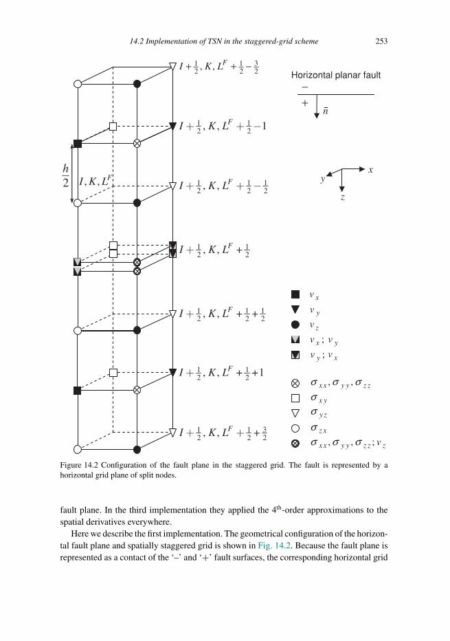
Trim: 247mm × 174mm Top: 14.762mm Gutter: 23.198mmCUUK2497-14 CUUK2497/Moczo ISBN: 978 1 107 02881 4 November 18, 2013 19:6
14.2 Implementation of TSN in the staggered-grid scheme 253
Figure 14.2 Configuration of the fault plane in the staggered grid. The fault is represented by ahorizontal grid plane of split nodes.
fault plane. In the third implementation they applied the 4th-order approximations to thespatial derivatives everywhere.
Here we describe the first implementation. The geometrical configuration of the horizon-tal fault plane and spatially staggered grid is shown in Fig. 14.2. Because the fault plane isrepresented as a contact of the ‘–’ and ‘+’ fault surfaces, the corresponding horizontal grid
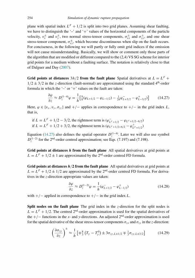
Trim: 247mm × 174mm Top: 14.762mm Gutter: 23.198mmCUUK2497-14 CUUK2497/Moczo ISBN: 978 1 107 02881 4 November 18, 2013 19:6
254 Simulation of dynamic rupture propagation
plane with spatial index LF + 1/2 is split into two grid planes. Assuming shear faulting,we have to distinguish the ‘–’ and ‘+’ values of the horizontal components of the particlevelocity, v±
x and v±y , two normal stress-tensor components, σ±
xx and σ±yy , and one shear
stress-tensor component, σ±xy , which become discontinuous when slip on the fault occurs.
For conciseness, in the following we will partly or fully omit grid indices if the omissionwill not cause misunderstanding. Basically, we will show or comment only those parts ofthe algorithm that are modified or different compared to the (2,4) VS SG scheme for interiorgrid points for a medium without a faulting surface. The notation is relatively close to thatof Dalguer and Day (2007).
Grid points at distances 3h/2 from the fault plane Spatial derivatives at L = LF +1/2 ± 3/2 in the z-direction (fault-normal) are approximated using the standard 4th-orderformula in which the ‘–’ or ‘+’ values on the fault are taken:
∂ϕ
∂z≈ D(1−4)
z ϕ = 1
h
[98 (ϕL+1/2 − ϕL−1/2) − 1
24ϕ−L+3/2 − ϕ+
L−3/2)]
(14.27)
Here, ϕ ∈ {vx, vy, σzz } and +/− applies in correspondence to +/− in the grid index L,that is,
if L = LF + 1/2 − 3/2, the rightmost term is (ϕ−LF+1/2 − ϕLF+1/2−6/2)
if L = LF + 1/2 + 3/2, the rightmost term is (ϕLF+1/2+6/2 − ϕ+LF+1/2)
Equation (14.27) also defines the spatial operator D(1−4)z . Later we will also use symbol
D(1−2)z for the 2nd-order centred approximation; see Eqs. (7.197) and (7.198).
Grid points at distances h from the fault plane All spatial derivatives at grid points atL = LF + 1/2 ± 1 are approximated by the 2nd-order centred FD formula.
Grid points at distances h/2 from the fault plane All spatial derivatives at grid points atL = LF + 1/2 ± 1/2 are approximated by the 2nd-order centred FD formula. For deriva-tives in the z-direction appropriate values are taken:
∂ϕ
∂z≈ D(1−2)
z ϕ = 1
h(ϕ−L+1/2 − ϕ+
L−1/2) (14.28)
with +/− applied in correspondence to +/− in the grid index L.
Split nodes on the fault plane The grid index in the z-direction for the split nodes isL = LF + 1/2. The centred 2nd-order approximation is used for the spatial derivatives ofthe +/− functions in the x- and y-directions. An adjusted 2nd-order approximation is usedfor the spatial derivative of the shear stress-tensor components σzx and σzy in the z-direction:(
∂σzγ
∂z
)±≈ 1
h
[∓ 83
(Tγ − T 0
γ
)± 3σzγ,L±1/2 ∓ 13σzγ,L±3/2
](14.29)

Trim: 247mm × 174mm Top: 14.762mm Gutter: 23.198mmCUUK2497-14 CUUK2497/Moczo ISBN: 978 1 107 02881 4 November 18, 2013 19:6
14.2 Implementation of TSN in the staggered-grid scheme 255
Tγ and T 0γ are the components of the constraint traction on the fault and γ ∈ {x, y}. Then
approximations of the equations of motion for v±x and v±
y are
ρ± 1
�t
[v±,m+1/2γ − v±,m−1/2
γ
] = [D(1−2)x σ±,m
xγ +D(1−2)y σ±,m
yγ
]+(∂σzγ
∂z
)±,m(14.30)
Here ( ∂σzγ∂z
)± is defined by Eq. (14.29). The slip rate at time level m+ 1/2 is
sm+1/2γ = v+,m+1/2
γ − v−,m+1/2γ (14.31)
Then slip is obtained from
sm+1γ = smγ +�tsm+1/2
γ (14.32)
A value of the constraint traction �T c on the fault obtained under the condition of �sm+1/2 = 0defines the trial traction. For simplicity of notation here, let �T ct denote the shear componentof the trial traction, see Eqs. (14.12) and (14.22). The boundary conditions on the fault areenforced by
T cγ = T ctγ ; |T ct | ≤ S
T cγ =�T ct
| �T ct |S;∣∣ �T ct ∣∣ > S (14.33)
In evaluation of the trial traction at grid positions of the particle-velocity components, themissing components of the trial traction are obtained by interpolation:∣∣ �T ctI,K+1/2
∣∣2 = [T ctx,I,K+1/2
]2 + [14
(T cty,I+1/2,K + T cty,I−1/2,K + T cty,I+1/2,K+1 + T cty,I−1/2,K+1
)]2
(14.34)
and ∣∣ �T ctI+1/2,K
∣∣2 = [14
(T ctx,I,K+1/2 + T ctx,I+1,K+1/2 + T ctx,I,K−1/2 + T ctx,I+1,K−1/2
)]2
+ [T cty,I+1/2,K
]2(14.35)
The missing components of the slip rate in the evaluation of the slip-path length areinterpolated analogously.
Finally, the approximations for the temporal derivatives of the stress-tensor componentsare
σ±xy ≈ μ (D(1−2)
y v±x +D(1−2)
x v±y
)(14.36)
σ±γ γ ≈ λ±
[D(1−2)x v±
x +D(1−2)y v±
y +(∂vz
∂z
)±]+ 2μ±D(1−2)
γ v±γ (14.37)

Trim: 247mm × 174mm Top: 14.762mm Gutter: 23.198mmCUUK2497-14 CUUK2497/Moczo ISBN: 978 1 107 02881 4 November 18, 2013 19:6
256 Simulation of dynamic rupture propagation
and
σ±zz ≈ λ±
[D(1−2)x v±
x +D(1−2)y v±
y +(∂vz
∂z
)±]+ 2μ±
(∂vz
∂z
)±(14.38)
where the adjusted 2nd-order approximation is used for the z-derivative:(∂vz
∂z
)±≈ 1
h
[∓ 83vz ± 3vz,L±1/2 ∓ 1
3vz,L±3/2]
(14.39)
Values of the continuous z-component of the particle velocity on the fault,
vz = vz,I+1/2,K+1/2,LF+1/2 (14.40)
are determined from the 2nd-order approximation to the boundary condition:(σ+zz = σ−
zz
)LF+1/2 (14.41)
The algorithms of the second and third implementations are relatively more complicatedand we will not detail them here. For a numerical comparison of the three implementationssee Moczo et al. (2007a), Section 11.3.
We did not introduce any artificial damping in the FD schemes. Dalguer and Day(2007) introduced viscous damping into the equations of motion in order to suppress short-wavelength oscillations arising from the numerical dispersion characteristic for a low-order FD approximation. Alternatively, the oscillations can be reduced using the adaptivesmoothing algorithm, see Section 17.3.
14.3 Initiation of spontaneous rupture propagation
Numerical simulations of rupture propagation under the linear slip-weakening friction lawrequire artificial procedures to initiate spontaneous rupture propagation. A frequently usedtechnique is based on imposing stress asperity. The effects of this artificial initiation dependon the geometry and size of the asperity, the spatial distribution of the stress in and aroundthe asperity, and a maximum overstress value. It is necessary to understand and minimizethe effects of artificial initiation on the subsequent spontaneous rupture propagation.
Numerical and analytical studies show that the size of the asperity should be chosenas small as possible. If an initiation zone is too small, rupture will not propagate or willterminate spontaneously at a finite distance from the nucleation region. On the other hand,if the initiation zone is too large it may strongly affect rupture propagation. Criteria forestimating the minimum size have been proposed for 2D in-plane and anti-plane rupturemodes (Andrews 1976a,b, Campillo and Ionescu 1997, Favreau et al. 1999, Uenishi andRice 2003) and for 3D (Day 1982, Uenishi and Rice 2004). Other studies (e.g., Galis et al.2010, Bizzarri 2010) suggest that these estimates do not provide general rules for designing3D simulations.
A variety of geometries/shapes of the initiation zone have been used for 3D dynamicrupture simulations. A square initiation patch has frequently been chosen (e.g., Harris et al.

Trim: 247mm × 174mm Top: 14.762mm Gutter: 23.198mmCUUK2497-14 CUUK2497/Moczo ISBN: 978 1 107 02881 4 November 18, 2013 19:6
14.3 Initiation of spontaneous rupture propagation 257
2009). Uenishi and Rice (2004), Dunham (2007), Galis et al. (2010) and Bizzarri (2010)suggested an elliptical initiation zone, while Ripperger et al. (2007) tested arbitrarily shapedinitiation regions.
Within the stress asperity the initial stress is chosen larger than the yield stress. Theoverstress (difference between the initial stress and yield stress) inside the asperity isassumed small, usually not larger than 1% over the static stress. Note that quantifying ofthe overstress by a percentage of the static stress does not lead to proper scaling of theoverstress with the stress drop and strength excess. For example, two configurations withequal stress drops and strength excesses but with different initial stresses should provide thesame results. Consider overstress quantified as a percentage of the static stress. Assumptionof the same percentage in both configurations then leads to different overstresses in MPa(because initial stress and consequently also static stress are different in the configurations)which eventually leads to different results. Therefore, it is reasonable to quantify theoverstress independently of the initial stress – by percentage of the difference between thestatic and dynamic stresses.
Most published studies that use stress-asperity parameterization for rupture initiationassume a stress discontinuity at the asperity edge: the asperity stress suddenly drops tothe level of the initial background stress. Two recent studies applied a smooth spatialdistribution of stress in and around the asperity (Galis et al. 2010, Bizzarri 2010).
Recently, Bizzarri (2010) tested different rupture initiation techniques, and showed that(a) forced rupture propagation with a proper rupture velocity leads to a gradual transitionfrom imposed initiation to spontaneous rupture propagation, (b) an elliptical stress asperitywith smooth stress is a valid alternative to forced rupture-propagation initiation. Bizzarri(2010) did not address the size of the initiation zone or overstress value.
Galis et al. (2013) performed extensive numerical simulations of 3D rupture propagationgoverned by the linear slip-weakening friction law (see Subsection 4.1.2). They consideredsquare, elliptical and circular shapes of the initiation zone with constant overstress, 0.5% ofτs − τ0, and values of the strength parameter S = (τs − τ0)/(τ0 − τd ) from 0.1 to 2.0. Theyfound that the area of the initiation zone, for given values of S and overstress, determineswhether the rupture will spontaneously propagate or not regardless of the particular shape ofthe initiation zone; see Fig. 14.3. The transition between propagating and non-propagatingruptures can be approximated by the curve
Ainit = 1.75S2.81 + 3.82 (14.42)
Here Ainit = A/L2fric is the dimensionless area of the initiation zone determined by area A
of the initiation zone in metres and parameter Lfric = μDc/(τs − τd ) proposed by Dunham(2007).
Galis et al. (2013) also presented the analytical formula derived using theoretical argu-ments:
A′init = (3π )3
211
τ0 − τdτi − τ0
(τs − τd )2
(τ0 − τd )4μ2D2
c (14.43)
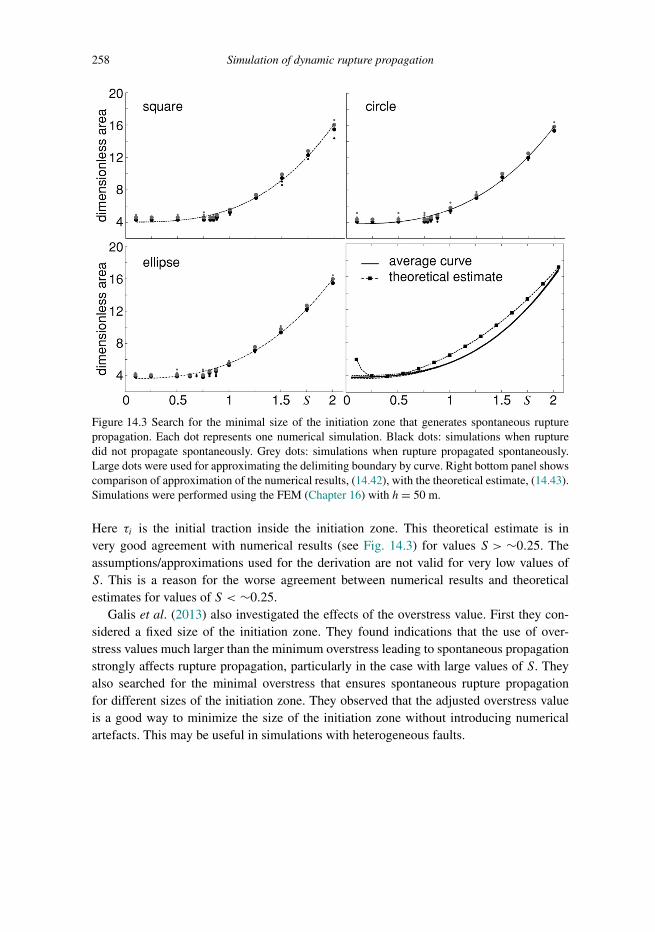
Trim: 247mm × 174mm Top: 14.762mm Gutter: 23.198mmCUUK2497-14 CUUK2497/Moczo ISBN: 978 1 107 02881 4 November 18, 2013 19:6
258 Simulation of dynamic rupture propagation
Figure 14.3 Search for the minimal size of the initiation zone that generates spontaneous rupturepropagation. Each dot represents one numerical simulation. Black dots: simulations when rupturedid not propagate spontaneously. Grey dots: simulations when rupture propagated spontaneously.Large dots were used for approximating the delimiting boundary by curve. Right bottom panel showscomparison of approximation of the numerical results, (14.42), with the theoretical estimate, (14.43).Simulations were performed using the FEM (Chapter 16) with h = 50 m.
Here τi is the initial traction inside the initiation zone. This theoretical estimate is invery good agreement with numerical results (see Fig. 14.3) for values S > ∼0.25. Theassumptions/approximations used for the derivation are not valid for very low values ofS. This is a reason for the worse agreement between numerical results and theoreticalestimates for values of S < ∼0.25.
Galis et al. (2013) also investigated the effects of the overstress value. First they con-sidered a fixed size of the initiation zone. They found indications that the use of over-stress values much larger than the minimum overstress leading to spontaneous propagationstrongly affects rupture propagation, particularly in the case with large values of S. Theyalso searched for the minimal overstress that ensures spontaneous rupture propagationfor different sizes of the initiation zone. They observed that the adjusted overstress valueis a good way to minimize the size of the initiation zone without introducing numericalartefacts. This may be useful in simulations with heterogeneous faults.

Trim: 247mm × 174mm Top: 14.762mm Gutter: 23.198mmCUUK2497-15 CUUK2497/Moczo ISBN: 978 1 107 02881 4 November 18, 2013 16:58
15
Preparation of computations and acomputational algorithm
(1) Input data� spatial distribution of
� P-wave and S-wave speeds� density� quality factorsQP andQS (orQκ andQμ)
� source and receiver positions� type of source, source-time function
(2) Determination of computational parameters� grid spacing from the maximum frequency up to which the simulation should be
accurate at a desired level (the size of the computational domain relates to theminimum frequency)
� time step from stability condition� number of time levels� parameters of PML
(3) Building computational model� coverage of the computational domain with a discontinuous grid� calculation of effective material grid parameters
(4) Algorithm of the computer code� reading input control parameters� reading computational model (grid model)� reading source-time function and source parameters� time loop (for determined number of time levels)
� calculation of strain rates from particle velocities� inside model� in PML� near and at the free surface
� update of anelastic functions from strain rates� update of stresses from strain rates and anelastic functions
259

Trim: 247mm × 174mm Top: 14.762mm Gutter: 23.198mmCUUK2497-15 CUUK2497/Moczo ISBN: 978 1 107 02881 4 November 18, 2013 16:58
260 Preparation of computations and a computational algorithm
� update of particle velocities� inside model� in PML� near and at the free surface
� application of source� storing seismograms and/or snapshots
(5) Post-processing of the simulated motion (low-pass or band-pass filtration)
It is necessary to perform numerical simulations for at least two different discretizations,e.g., for two sizes of the spatial grid spacing, in order to assess the sensitivity of thesimulated motion with respect to the computational parameters.

Trim: 247mm × 174mm Top: 14.762mm Gutter: 23.198mmCUUK2497-16 CUUK2497/Moczo ISBN: 978 1 107 02881 4 November 18, 2013 18:59
Part IIIFinite-element method and hybrid
finite-difference–finite-element method

Trim: 247mm × 174mm Top: 14.762mm Gutter: 23.198mmCUUK2497-16 CUUK2497/Moczo ISBN: 978 1 107 02881 4 November 18, 2013 18:59
Trim: 247mm × 174mm Top: 14.762mm Gutter: 23.198mmCUUK2497-16 CUUK2497/Moczo ISBN: 978 1 107 02881 4 November 18, 2013 18:59
16
Finite-element method
Detailed expositions of the FEM and its application to a variety of problems can be found inbooks such as those by Strang and Fix (1988), Zienkiewicz and Taylor (1989), Ottosen andPetersson (1992), Belytschko el al. (2000), Hughes (2000), Felippa (2005), Reddy (2006).
The purpose of this chapter is to briefly introduce the basics of the FEM and explain ourefficient implementation based on the global restoring-force vector with significantly lowermemory requirements as compared to the requirements of the global stiffness matrix. Wealso use so-called e-invariants for efficient computation of the restoring-force vector. Thechapter will provide a basis for later expositions of FE modelling of rupture propagationand the hybrid FD–FE method.
Unlike most chapters on the FDM, here we indicate the spatial and temporal derivatives,respectively, as
ϕi,j ≡ ∂ϕi
∂xj, ϕi ≡ ∂ϕi
∂t(16.1)
We choose this notation in order to have the equations in a concise form.
16.1 Weak form of the equation of motion
Consider a domain � = � ∪ �, where� is an interior and � its boundary. We assume thatboundary � can be decomposed into two parts, �D and �N , without overlapping, that is,�D ∩ �N = ∅ (see Fig. 16.1). We assume a prescribed displacement vector at boundary �Dand prescribed traction at boundary �N . Recall the strong-form equation of motion (2.7):
ρui = σij,j + fi (16.2)
and boundary condition (2.8) at �N :
σij (�x)nj (�x) = hi ; �x ∈ �N (16.3)
where �n(�x) is an outer normal. Here we also consider the boundary condition at �D:
ui (�x, t) = gi (�x, t) ; �x ∈ �D (16.4)
263
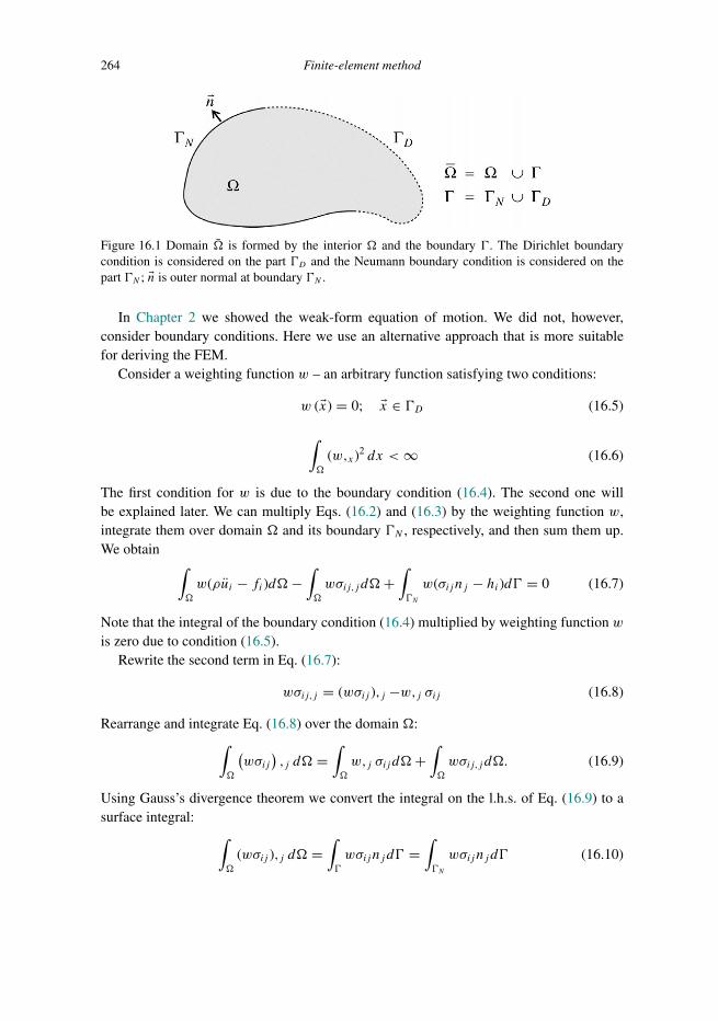
Trim: 247mm × 174mm Top: 14.762mm Gutter: 23.198mmCUUK2497-16 CUUK2497/Moczo ISBN: 978 1 107 02881 4 November 18, 2013 18:59
264 Finite-element method
Figure 16.1 Domain � is formed by the interior � and the boundary �. The Dirichlet boundarycondition is considered on the part �D and the Neumann boundary condition is considered on thepart �N ; �n is outer normal at boundary �N .
In Chapter 2 we showed the weak-form equation of motion. We did not, however,consider boundary conditions. Here we use an alternative approach that is more suitablefor deriving the FEM.
Consider a weighting function w – an arbitrary function satisfying two conditions:
w (�x) = 0; �x ∈ �D (16.5)
∫�
(w,x)2 dx <∞ (16.6)
The first condition for w is due to the boundary condition (16.4). The second one willbe explained later. We can multiply Eqs. (16.2) and (16.3) by the weighting function w,integrate them over domain � and its boundary �N , respectively, and then sum them up.We obtain ∫
�
w(ρui − fi)d�−∫�
wσij,j d�+∫�N
w(σijnj − hi)d� = 0 (16.7)
Note that the integral of the boundary condition (16.4) multiplied by weighting function wis zero due to condition (16.5).
Rewrite the second term in Eq. (16.7):
wσij,j = (wσij ),j −w,j σij (16.8)
Rearrange and integrate Eq. (16.8) over the domain �:∫�
(wσij
),j d� =
∫�
w,j σij d�+∫�
wσij,j d�. (16.9)
Using Gauss’s divergence theorem we convert the integral on the l.h.s. of Eq. (16.9) to asurface integral: ∫
�
(wσij ),j d� =∫�
wσijnjd� =∫�N
wσijnjd� (16.10)

Trim: 247mm × 174mm Top: 14.762mm Gutter: 23.198mmCUUK2497-16 CUUK2497/Moczo ISBN: 978 1 107 02881 4 November 18, 2013 18:59
16.2 Discrete weak form of the equation of motion 265
where we used the property (16.5) of the weighting functionw. Now we can use Eqs. (16.9)and (16.10) to express the second term of Eq. (16.7):∫
�
wσij,j d� =∫�N
wσijnjd� −∫�
w,j σij d� (16.11)
Eventually, using Eq. (16.11) we rewrite Eq. (16.7):∫�
w (ρui − fi) d�+∫�
w,j σij d�−∫�N
whid� = 0 (16.12)
For the equation to be meaningful the integrals must be well defined. That imposesconditions on solution ui . Moreover, the solution ui has to satisfy the boundary condition(16.4). The conditions on solution ui of Eq. (16.12) are weaker than of the strong-formEq. (16.2). For example, the weak form allows solutions ui to be piece-wise linear functions.The piece-wise linear functions cannot be solutions of the strong-form equation becausethe derivatives are not well defined. Therefore Eq. (16.12) is called the weak form of theequation of motion. Note that Eq. (16.12) has to be satisfied for an arbitrary weightingfunction w. Consequently, Eq. (16.12) represents, in fact, three infinite sets of equations(one set for each component of solution). To solve Eq. (16.12) in practical applications wehave to consider only a finite set of weighting functions.
16.2 Discrete weak form of the equation of motion for an element
We can imagine an element as a domain with a simple geometric shape with nodes in thevertices, e.g., tetrahedron, hexahedron or pyramid. In the next section we define the elementusing shape functions. Assume an element with n nodes. Assign numbers or indices to nodesso that each node can be referred to by a number from a set ν ≡ {1, . . . , n}. Then we candefine a set νD ⊂ ν as a set of indices of nodes on boundary �D at which the displacementvector is prescribed. Similarly, we can define a complementary set ν\νD as a set of the freenodes at which the displacement vector is not prescribed. Correspondingly, nD denotes thenumber of the nodes with prescribed displacement and n− nD denotes the number of thefree nodes.
Now recall the weak form of the equation of motion (16.12). Further, we assume oneand the same set of weighting functions for all three components of displacement.
We can define a finite set of the weighting functions Sw as
Sw ≡ {sl|l ∈ ν\νD} (16.13)
This means that the weighting functions are from a finite set of n− nD functions, sl ,defined only for nodes not lying on boundary �D . No weighting functions are defined fornodes on boundary �D . Note that functions from Sw are zero on �D – in accordance with(16.5).
In general, we can consider the solution approximated by a linear combination of shapefunctions, which may be different from weighting functions. Here, we limit the discussion
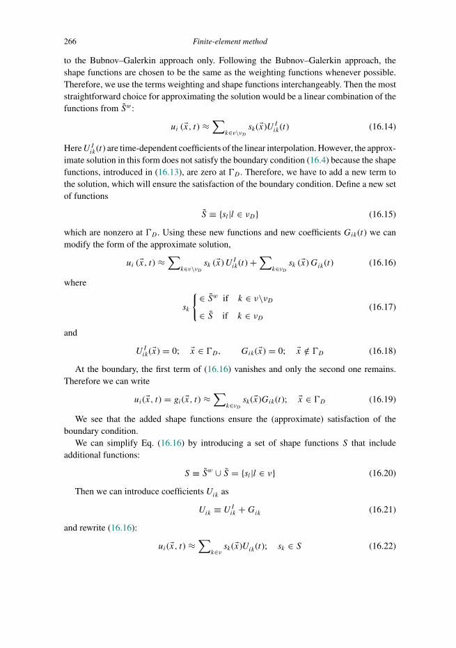
Trim: 247mm × 174mm Top: 14.762mm Gutter: 23.198mmCUUK2497-16 CUUK2497/Moczo ISBN: 978 1 107 02881 4 November 18, 2013 18:59
266 Finite-element method
to the Bubnov–Galerkin approach only. Following the Bubnov–Galerkin approach, theshape functions are chosen to be the same as the weighting functions whenever possible.Therefore, we use the terms weighting and shape functions interchangeably. Then the moststraightforward choice for approximating the solution would be a linear combination of thefunctions from Sw:
ui (�x, t) ≈∑
k∈ν\νDsk(�x)UIik(t) (16.14)
HereUIik(t) are time-dependent coefficients of the linear interpolation. However, the approx-imate solution in this form does not satisfy the boundary condition (16.4) because the shapefunctions, introduced in (16.13), are zero at �D . Therefore, we have to add a new term tothe solution, which will ensure the satisfaction of the boundary condition. Define a new setof functions
S ≡ {sl|l ∈ νD} (16.15)
which are nonzero at �D . Using these new functions and new coefficients Gik(t) we canmodify the form of the approximate solution,
ui (�x, t) ≈∑
k∈ν\νDsk (�x)UIik(t) +
∑k∈νD
sk (�x)Gik(t) (16.16)
where
sk
{∈ Sw if k ∈ ν\νD∈ S if k ∈ νD
(16.17)
and
UIik(�x) = 0; �x ∈ �D, Gik(�x) = 0; �x /∈ �D (16.18)
At the boundary, the first term of (16.16) vanishes and only the second one remains.Therefore we can write
ui(�x, t) = gi(�x, t) ≈∑
k∈νDsk(�x)Gik(t); �x ∈ �D (16.19)
We see that the added shape functions ensure the (approximate) satisfaction of theboundary condition.
We can simplify Eq. (16.16) by introducing a set of shape functions S that includeadditional functions:
S ≡ Sw ∪ S = {sl|l ∈ ν} (16.20)
Then we can introduce coefficients Uik as
Uik ≡ UIik +Gik (16.21)
and rewrite (16.16):
ui(�x, t) ≈∑
k∈ν sk(�x)Uik(t); sk ∈ S (16.22)

Trim: 247mm × 174mm Top: 14.762mm Gutter: 23.198mmCUUK2497-16 CUUK2497/Moczo ISBN: 978 1 107 02881 4 November 18, 2013 18:59
16.3 Shape functions 267
We can also extend the set of weighting functions. The extended set of weightingfunctions Sw includes zero functions for nodes on boundary �D and shape functions for allother nodes. Let
sl
{≡ sl, l ∈ ν\νD≡ 0, l ∈ νD
(16.23)
Then,
Sw ≡ {sl|l ∈ ν} (16.24)
We illustrate function sets Sw, Sw, S and S using a simple example. Consider the 2Dquadrilateral element with four nodes in the vertices. Denote them 1, 2, 3 and 4. Assume aprescribed displacement at node 3. Then set Sw , defined by (16.13), will be Sw = {s1, s2, s4}.The s3 is missing. Set S, defined by Eq. (16.15), will be S = {s3}. Then, according to (16.20)and (16.24), S = {s1, s2, s3, s4} and Sw = {s1, s2, 0, s4}, respectively.
Assuming the finite set of weighting functions (16.24) and assuming the approximatesolution (16.22), we can rewrite the weak-form equation (16.12):∫
�
wk(ρslUil − fi
)d�+
∫�
wk,jσij d�−∫�N
wkhid� = 0 (16.25)
Here k, l ∈ ν, wk ∈ Sw and sl ∈ S. We obtain three finite sets of n− nD equations forn− nD unknown coefficients Uil (the l.h.s. will be zero for k ∈ νD). This is a discreteor Galerkin weak form. Note that the Galerkin form includes the boundary conditions at�D . Note also that the stress tensor σij implicitly depends on the spatial derivatives ofdisplacement and consequently on the spatial derivatives of the shape functions. Condition(16.6) thus guarantees the existence of the second integral on the l.h.s. of (16.25).
Before we continue with the derivation of a matrix form of Eq. (16.25) we define theshape functions.
16.3 Shape functions
The properties of a final FE scheme very much depend on the choice of shape functions. Toobtain the converging scheme the shape functions must be smooth inside an element, con-tinuous at boundaries between elements, and complete. The first two conditions guaranteethat the integrals in the discrete weak form, Eq. (16.25), are well defined. The second con-dition may be physically interpreted as the requirement of displacement continuity acrosselements. According to the third condition, the shape functions must be able to exactlyrepresent linear polynomials inside the element. This may be physically interpreted as therequirement of exact representation of the constant-strain state inside an element.
So far we have considered only one element. Next we consider the whole domain �covered by elements without holes and overlapping.
In general, the shape functions may be defined in the whole domain. In the case of a largenumber of elements and nodes this approach is very expensive because it leads to functions

Trim: 247mm × 174mm Top: 14.762mm Gutter: 23.198mmCUUK2497-16 CUUK2497/Moczo ISBN: 978 1 107 02881 4 November 18, 2013 18:59
268 Finite-element method
(a) (b)
x
y
2 2[ , ]x y1 1[ , ]x y
3 3[ , ]x y4 4[ , ]x y
ξ
η[ 1, 1]− + [ 1, 1]+ +
[ 1, 1]− − [ 1, 1]+ −1 2
4 3
Figure 16.2 Transformation from the local to the physical coordinates in 2D. Left: a reference element�ref in the local coordinates (ξ, η). Right: an element in the physical coordinates (x, y).
of very high order. It is better to use shape functions defined per element. In this case wecan use low-order functions and still have a reasonable approximation of the solution inthe whole domain. For simplicity, consider a 1D example. Consider linear shape functionsper element. In such a case the solution in one element will be approximated by a linearfunction (see Eq. (16.22)). If we cover the whole domain with more elements, the solutionin the domain will be approximated by a piece-wise linear function.
In addition to the local shape functions, it may be useful to transform elements fromthe physical coordinates (x, y, z) into the local coordinates (ξ, η, ζ ), and define the shapefunctions in the local coordinates. Consequently, the shape functions for all elements willhave the same form in the local coordinates. This means that for a given type of elementwe have to derive the shape functions only once. For simplicity, we first derive and presentthe shape functions for a quadrilateral element in 2D and then for a hexahedral elementin 3D.
Assume a reference element �ref as a square element in the local coordinate system(ξ, η) as shown in Fig. 16.2. The nodes are at positions
�ξ ≡ (−1, 1, 1,−1) , �η ≡ (−1,−1, 1, 1) (16.26)
We need to define four shape functions for set S. These functions are used to approximatethe solution ui (�x, t). We can find them by solving the system of equations
sk(ξl, ηl) = δkl ; k, l = 1, 2, 3, 4 (16.27)
where δkl is the Kronecker delta. The system consists of four equations for each shapefunction. Therefore, to make system (16.27) uniquely solvable, the shape functions musthave four parameters. We will consider shape functions in the form
sk(ξ, η) = akξ + bkη + ckξη + dk, k = 1, 2, 3, 4 (16.28)
After solving the system (16.27) for shape functions in the form (16.28) the shape functionscan be written as
s1(ξ, η) = 14 (1 − ξ )(1 − η), s2(ξ, η) = 1
4 (1 + ξ )(1 − η)
s3(ξ, η) = 14 (1 + ξ )(1 + η), s4(ξ, η) = 1
4 (1 − ξ )(1 + η)(16.29)

Trim: 247mm × 174mm Top: 14.762mm Gutter: 23.198mmCUUK2497-16 CUUK2497/Moczo ISBN: 978 1 107 02881 4 November 18, 2013 18:59
16.3 Shape functions 269
These functions are called bilinear because for fixed η we obtain a linear function ofξ , and vice versa, for fixed ξ we obtain a linear function of η. Note that the consequenceof using shape functions satisfying the system of equations (16.27) is that coefficient Uilrepresents the i-th component of displacement at node l.
The formation of the function set Sw is also straightforward. This set contains onlythose shape functions from set S that are not associated with nodes on boundary �D . Thefunctions from S associated with nodes at �D are replaced with zeros, as indicated byEq. (16.23). Moreover, the functions from Sw have to be zero at �D . This condition isimplicitly satisfied for the shape functions in Sw as a consequence of Eq. (16.27).
For practical use of the shape functions in the local coordinates we need a transformationfrom the local to the physical coordinates. In general, if a function is given at the nodes ofan element, we can use shape functions to interpolate the function in the element. We canuse this approach to express the transformation from the local to the physical coordinatesas
x = xksk(ξ, η), y = yksk (ξ, η) (16.30)
where xk and yk are the x- and y-positions of the nodes in the physical coordinates. We canuse the local coordinates if the transformation is unique for the element. The transformation(16.30) exists and is unique if the element in the physical coordinates has the shape of aconvex quadrilateral, that is, if each of the inner angles is smaller than 180°, and the methodof numbering the nodes in the global and local coordinates is the same. Figure 16.3a showsan element in the local coordinates with the nodes numbered counterclockwise. Figure 16.3bshows the case of a well-shaped element with correct numbering and, consequently, with aunique transformation. Figure 16.3c illustrates a nonunique transformation due to a differentnumbering order in the local and physical coordinates. The nonunique transformation inFig. 16.3d is due to an element with the inner angle at node 4 larger than 180°.
Earlier we mentioned conditions for the shape functions. We now check whether theshape functions (16.29) satisfy all conditions. The shape functions (16.29) are obviouslysmooth and continuous inside an element. Is the solution approximated using the shapefunctions (16.29) continuous across two elements? Consider the situation in Fig. 16.4.A solution in two quadrilateral elements is approximated by bilinear functions in eachelement. The solution is defined at nodes regardless of which element we are looking at.Therefore, we have to check only the behaviour of the shape functions at the contact ofthe elements, between nodes 2 and 5. Due to bilinearity, the solution on the edge of theelement is a linear function uniquely defined by solution at nodes 2 and 5. Consequently,the linear function at the contact of two elements is the same for both elements and thesolution is continuous across the elements. This is true for any two quadrilateral elementswith bilinear shape functions. The last of the requirements was exact representation of theconstant strain or, in other words, exact representation of linear polynomials. Consider thelinear function
f (x, y) = ax + by + c (16.31)

Trim: 247mm × 174mm Top: 14.762mm Gutter: 23.198mmCUUK2497-16 CUUK2497/Moczo ISBN: 978 1 107 02881 4 November 18, 2013 18:59
270 Finite-element method
-1 -0.5 0 0.5 1
-1
-0.5
0
0.5
1η
ξ
4 3
21
-2 0 2 4 6
-2
0
2
4
6
-2 0 2 4 6
-2
0
2
4
6
-2 0 2 4 6
-2
0
2
4
6
x
y
(b)
(c) (d)
(a)
4
3
2
1
xx
yy
3
4
2
1
4
3
2
1
Figure 16.3 Example of transformations from the local to the physical coordinates in 2D: (a) referenceelement in the local coordinates, (b) unique transformation to a convex quadrilateral, (c) nonuniquetransformation caused by wrong node numbering, (d) nonunique transformation to a nonconvexquadrilateral.
The values of this function at nodes of the element will be
F1 = ax1 + by1 + c, F2 = ax2 + by2 + cF3 = ax3 + by3 + c, F4 = ax4 + by4 + c
(16.32)
We use shape functions (16.29) to approximate function f (x, y) in one element:
f (x, y) ≈ s1F1 + s2F2 + s3F3 + s4F4 (16.33)

Trim: 247mm × 174mm Top: 14.762mm Gutter: 23.198mmCUUK2497-16 CUUK2497/Moczo ISBN: 978 1 107 02881 4 November 18, 2013 18:59
16.3 Shape functions 271
1
1
2
3
52
6
4
1U 2U
3U
4U
5U6U
Figure 16.4 Proof of the continuity of the displacement on the contact of two quadrilateral elementswith bilinear shape functions.
After using (16.31) in (16.32), and rearranging terms on the r.h.s. with respect to coeffi-cients a, b and c we obtain
f (x, y) ≈ a∑4
k=1skxk + b
∑4
k=1skyk + c
∑4
k=1sk (16.34)
Considering (16.30), the first sum is equal to x and the second sum is equal to y. It remainsto be shown that the last sum equals 1. This is straightforward if we use the definition ofthe shape functions (16.29). We can rewrite Eq. (16.33) as
f (x, y) ≈ ax + by + c (16.35)
and we see that the linear function f (x, y) is exactly represented by the shape functions.Now we can easily extend the 2D quadrilateral element into a 3D hexahedral element.
We assume a reference element,�ref , as a cube in the local coordinates (ξ, η, ζ ), Fig. 16.5.The nodes are at positions
�ξ ≡ (−1, 1, 1,−1,−1, 1, 1,−1)
�η ≡ (−1,−1, 1, 1,−1,−1, 1, 1)
�ζ ≡ (−1,−1,−1,−1, 1, 1, 1, 1)
(16.36)

Trim: 247mm × 174mm Top: 14.762mm Gutter: 23.198mmCUUK2497-16 CUUK2497/Moczo ISBN: 978 1 107 02881 4 November 18, 2013 18:59
272 Finite-element method
[ 1, 1, 1]− − − [ 1, 1, 1]+ − −
[ 1, 1, 1]− + −
[ 1, 1, 1]− − +
[ 1, 1, 1]+ + +[ 1, 1, 1]− + +
2 2 2[ , , ]x y z1 1 1[ , , ]x y z
4 4 4[ , , ]x y z
7 7 7[ , , ]x y z8 8 8[ , , ]x y z
x
yz
ξη
ζ
3 3 3[ , , ]x y z[ 1, 1, 1]+ + −
[ 1, 1, 1]+ − +
6 6 6[ , , ]x y z
(a) (b)
1 2
4 3
5 6
8 7
5 5 5[ , , ]x y z
Figure 16.5 Transformation from the local to the physical coordinates in 3D. Left: a reference element�ref in the local coordinates (ξ, η, ζ ). Right: an element in the physical coordinates (x, y, z).
Consider trilinear functions:
sk(ξ, η, ζ ) = akξ + bkη + ckζ + dkξη + ekηζ + fkξζ + gkξηζ + hk (16.37)
A linear function for ξ can be obtained from the trilinear function by fixing two remainingvariables η and ζ . Solving system (16.27) for k, l = 1, 2, . . . , 8 gives eight shape functions,which can be written as
sk(ξ, η, ζ ) = 18 (1 + ξkξ )(1 + ηkη)(1 + ζkζ ); k = 1, 2, . . . , 8 (16.38)
where ξk , ηk and ζk are components of vectors �ξ , �η and �ζ defined in Eq. (16.35). Thetransformation of the physical coordinates can be defined analogously with (16.30):
x = xksk(ξ, η, ζ ), y = yksk(ξ, η, ζ ), z = zksk(ξ, η, ζ ) (16.39)
Similarly to the 2D case, the element in the local coordinates may be used only iftransformation (16.38) exists and is unique. This means that the element has to havethe shape of a convex hexahedron and the nodes in the physical and local coordinates mustbe numbered in the same way.
We do not address the satisfaction of the requirements in the 3D case as it is a just simpleand straightforward extension of what we have shown in 2D.
In the following sections we will use the abbreviation HEX8 to denote the hexahedralelement with eight nodes and trilinear shape functions.
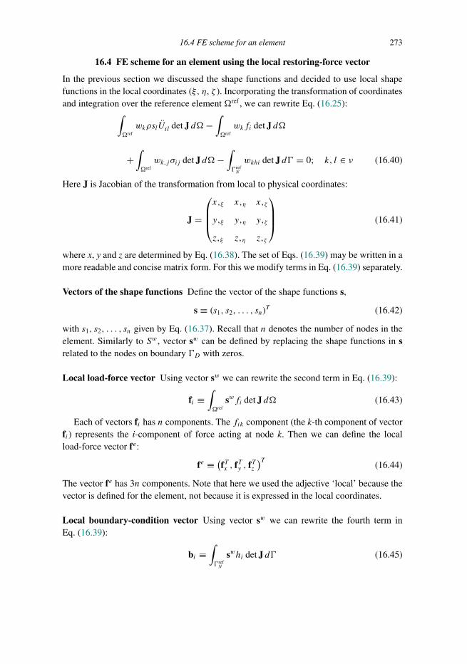
Trim: 247mm × 174mm Top: 14.762mm Gutter: 23.198mmCUUK2497-16 CUUK2497/Moczo ISBN: 978 1 107 02881 4 November 18, 2013 18:59
16.4 FE scheme for an element 273
16.4 FE scheme for an element using the local restoring-force vector
In the previous section we discussed the shape functions and decided to use local shapefunctions in the local coordinates (ξ, η, ζ ). Incorporating the transformation of coordinatesand integration over the reference element �ref , we can rewrite Eq. (16.25):∫
�refwkρslUil det J d�−
∫�refwkfi det J d�
+∫�refwk,jσij det J d�−
∫�refN
wkhi det J d� = 0; k, l ∈ ν (16.40)
Here J is Jacobian of the transformation from local to physical coordinates:
J =
⎛⎜⎜⎝x,ξ x,η x,ζ
y,ξ y,η y,ζ
z,ξ z,η z,ζ
⎞⎟⎟⎠ (16.41)
where x, y and z are determined by Eq. (16.38). The set of Eqs. (16.39) may be written in amore readable and concise matrix form. For this we modify terms in Eq. (16.39) separately.
Vectors of the shape functions Define the vector of the shape functions s,
s ≡ (s1, s2, . . . , sn)T (16.42)
with s1, s2, . . . , sn given by Eq. (16.37). Recall that n denotes the number of nodes in theelement. Similarly to Sw, vector sw can be defined by replacing the shape functions in srelated to the nodes on boundary �D with zeros.
Local load-force vector Using vector sw we can rewrite the second term in Eq. (16.39):
fi ≡∫�ref
swfi det J d� (16.43)
Each of vectors fi has n components. The fik component (the k-th component of vectorfi) represents the i-component of force acting at node k. Then we can define the localload-force vector fe:
fe ≡ (fTx , f
Ty , f
Tz
)T(16.44)
The vector fe has 3n components. Note that here we used the adjective ‘local’ because thevector is defined for the element, not because it is expressed in the local coordinates.
Local boundary-condition vector Using vector sw we can rewrite the fourth term inEq. (16.39):
bi ≡∫�refN
swhi det J d� (16.45)

Trim: 247mm × 174mm Top: 14.762mm Gutter: 23.198mmCUUK2497-16 CUUK2497/Moczo ISBN: 978 1 107 02881 4 November 18, 2013 18:59
274 Finite-element method
Each of the bi vectors has n components. The bik component (the k-component of vectorbi) represents the i-component of force acting at node k due to traction hi acting at �mN .Then we can define the local boundary-condition vector be:
be ≡ (bTx ,bTy ,b
Tz )T (16.46)
The vector be has 3n components.
Local mass matrix Now we focus on the first term in Eq. (16.39). Recall that Uil isconstant in space (being a function of time) and therefore we can rewrite the term:∫
�refwkρslUil det J d� =
∫�refwkρsl det J d�Uil (16.47)
Define a local mass matrix me as
me ≡
⎛⎜⎜⎝
me 0 0
0 me 0
0 0 me
⎞⎟⎟⎠ (16.48)
with matrices me defined as
me ≡∫�ref
swρsT det J d� (16.49)
The dimensions of me and the local mass matrix me are n× n and 3n× 3n, respectively.We define also a local vector of discrete displacements ue as
ue ≡[(
uex)T,(uey)T,(uez)T ]T
(16.50)
where
uei ≡ (Ui1, Ui2, . . . , Uin)T (16.51)
As mentioned before, Uil represents the i-component of displacement at node l.The dimensions of vectors uei are dimensions n× 1, dimensions of the local discrete-displacement vector are dimensions 3n× 1. Using the local mass matrix and discrete-displacement vector we can rewrite terms in (16.46) in matrix-vector notation:∫
�refwkρsl det J d�Uil → meue (16.52)
Local restoring-force vector for an elastic isotropic medium The FE formulation withthe concept of restoring forces at nodes considerably reduces memory requirements com-pared to the FE formulation with the global stiffness matrix. Our formulation and imple-mentation is based on the outline of the formulation presented by Archuleta (1976, andpersonal communication) who refers to Frazier and Petersen (1974).
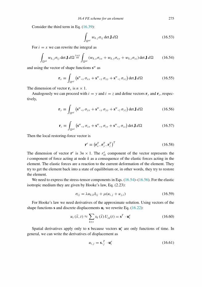
Trim: 247mm × 174mm Top: 14.762mm Gutter: 23.198mmCUUK2497-16 CUUK2497/Moczo ISBN: 978 1 107 02881 4 November 18, 2013 18:59
16.4 FE scheme for an element 275
Consider the third term in Eq. (16.39):∫�refwk,jσij det J d� (16.53)
For i = x we can rewrite the integral as∫�refwk,jσij det J d�
i=x=∫�ref
(wk,xσxx + wk,yσxy + wk,zσxz) det J d� (16.54)
and using the vector of shape functions sw as
rx ≡∫�ref
(sw,x σxx + sw,y σxy + sw,z σxz
)det J d� (16.55)
The dimension of vector rx is n× 1.Analogously we can proceed with i = y and i = z and define vectors ry and rz, respec-
tively,
ry ≡∫�ref
(sw,x σyx + sw,y σyy + sw,z σyz
)det J d� (16.56)
rz ≡∫�ref
(sw,x σzx + sw,y σzy + sw,z σzz
)det J d� (16.57)
Then the local restoring-force vector is
re ≡ (rTx , r
Ty , r
Tz
)T(16.58)
The dimension of vector re is 3n× 1. The reik component of the vector represents thei-component of force acting at node k as a consequence of the elastic forces acting in theelement. The elastic forces are a reaction to the current deformation of the element. Theytry to get the element back into a state of equilibrium or, in other words, they try to restorethe element.
We need to express the stress-tensor components in Eqs. (16.54)–(16.56). For the elasticisotropic medium they are given by Hooke’s law, Eq. (2.23):
σij = λuk,kδij + μ(ui,j + uj,i) (16.59)
For Hooke’s law we need derivatives of the approximate solution. Using vectors of theshape functions s and discrete displacements ui we rewrite Eq. (16.22):
ui (�x, t) ≈∑k∈νsk (�x)Uik(t) = sT · uei (16.60)
Spatial derivatives apply only to s because vectors uei are only functions of time. Ingeneral, we can write the derivatives of displacement as
ui,j = s,Tj · uei (16.61)

Trim: 247mm × 174mm Top: 14.762mm Gutter: 23.198mmCUUK2497-16 CUUK2497/Moczo ISBN: 978 1 107 02881 4 November 18, 2013 18:59
276 Finite-element method
Here we need derivatives with respect to the physical coordinates (x, y, z) but our shapefunctions are defined for the local coordinates (ξ, η, ζ ). Applying the chain rule leads to
s,x = s,ξ ξ,x + s,η η,x +s,ζ ζ,x
s,y = s,ξ ξ,y + s,η η,y +s,ζ ζ,y
s,z= s,ξ ξ,z+ s,η η,z+s,ζ ζ,z
(16.62)
The inverse Jacobian of transformation (16.38) is
J−1 =
⎛⎜⎜⎝ξ,x ξ,y ξ,z
η,x η,y η,z
ζ,x ζ,y η,z
⎞⎟⎟⎠ (16.63)
By comparing Eqs. (16.62) and (16.61) we see that we can use the correspondingcomponents of the inverse Jacobian to express derivatives of the local coordinates (ξ, η, ζ )with respect to the physical coordinates (x, y, z) needed in Eq. (16.61).
Note on computation of integrals To construct the local quantities we have to computevolume or surface integrals. For example, in the case of the local restoring-force vectorwe have to compute integrals (16.54)–(16.56). In general, numerical integration is used forthe HEX8 elements. To choose the correct order of numerical integration, one must analyzethe functions that are to be integrated. Gaussian integration is the most efficient integrationin terms of the lowest number of integration points needed to achieve the desired precision.Therefore, 8-point (2 points in each direction) Gaussian integration is usually used for theHEX8 elements. This integration is exact for up to cubic polynomials and therefore it isconsidered an exact integration for the undeformed elements (‘exact’ here means that theerror is caused only by a discrete representation of numbers). In the case of the deformedelements we may need to increase the order of integration due to the more complicatedform of det J. However, in general, the more deformed the element we use, the larger willbe the systematic error.
Sometimes it is reasonable to use integration with lower accuracy than what is requiredfor the exact integration. This may be due to higher efficiency (lower accuracy of integrationmay mean fewer integration points and consequently fewer operations) or due to differentproperties of the final scheme. For better efficiency, 1-point Gaussian integration is oftenused with the HEX8 elements (e.g., Ma and Liu 2006). However, note that the scheme basedon the 1-point Gaussian integration has to be used with algorithms for reducing hourglassmodes. Otherwise it will provide unusable results. See Chapter 17 for an example of thereduced integration.

Trim: 247mm × 174mm Top: 14.762mm Gutter: 23.198mmCUUK2497-16 CUUK2497/Moczo ISBN: 978 1 107 02881 4 November 18, 2013 18:59
16.4 FE scheme for an element 277
Local restoring-force vector for an isotropic medium with realistic attenuation Herewe will address the implementation of realistic attenuation based on the rheology of GMB-EK/GZB into the FEM. The general procedure is the same as for the elastic case, thedifference is only in the type of stress–strain relation adopted.
In Chapter 3 we derived stress–strain relations for a 3D viscoelastic continuum usingthe GMB-EK/GZB. Recall the stress–strain relation, Eq. (3.134):
σij = κεkkδij + 2μ(εij − 1
3εkkδij)−
∑nl
l=1
[Y κl κζ
kkl δij + 2Yμl μ
(ζijl − 1
3ζkkl δij
)](16.64)
where κ and μ are the unrelaxed bulk and shear modulus, respectively, Y κl and Yμl arecorresponding anelastic coefficients, defined by Eqs. (3.140), and ζ ijl are anelastic functionsdefined by the differential equation, see Eq. (3.135):
ζijl + ωlζ ijl = ωlεij (16.65)
Recall that indices i, j and k are spatial indices and therefore i, j, k ∈ {1, 2, 3}. Indexl is related to the relaxation frequencies and therefore l ∈ {1, 2, . . . , nl}. The summationconvention does not apply to index l. We can rewrite the stress–strain relation (16.63) in aform more suitable for implementation in the FEM:
σij = σEij −∑nl
l=1σAlij (16.66)
Here σEij and σAlij denote the elastic and anelastic parts, respectively. The anelastic partsmay be defined by
σAlxx = Y+ζ xxl + Y−ζ yyl + Y−ζ zzl
σAlyy = Y−ζ xxl + Y+ζ yyl + Y−ζ zzl
σAlzz = Y−ζ xxl + Y−ζ yyl + Y+ζ zzl
σAlxy = 2μYμl ζxyl
σAlyz = 2μYμl ζyzl
σAlxz = 2μYμl ζxzl
(16.67)
where Y+ = κY κl + 43μY
μl and Y− = κY κl − 2
3μYμl . The anelastic functions are obtained
from Eq. (16.64) as follows (Kristek and Moczo 2003). The temporal derivative of ζ ijl (t) isapproximated by the 2nd-order central difference formula. Function ζ ijl (t) itself is approxi-mated as the arithmetic average:
ζijl (t) = 1
2
[ζijl (t − 1
2�t) + ζ ijl(t + 1
2�t)]
(16.68)
Finally, we obtain the recurrent formula:
ζijl
(t + 1
2�t) = 2ωl�tεij (t) + (2 − ωl�t)ζ ijl
(t − 1
2�t)
2 + ωl�t (16.69)

Trim: 247mm × 174mm Top: 14.762mm Gutter: 23.198mmCUUK2497-16 CUUK2497/Moczo ISBN: 978 1 107 02881 4 November 18, 2013 18:59
278 Finite-element method
We use (16.68) to obtain ζ ijl(t + 1
2�t)
and then (16.67) to obtain ζ ijl (t). (Compare withthe algorithm for the velocity–stress staggered-grid scheme in Section 7.8.)
As we have already discussed, numerical integration is used to compute the localrestoring-force vector. This implies that anelastic functions are required at all integra-tion points. Moreover, the recurrent formula (16.68) implies that the anelastic functionshave to be stored in computer memory. That would cause drastic memory requirementsand consequently the computations for a viscoelastic medium would be impossible formany realistic problems. To reduce the memory requirements down to a feasible level weevaluate the anelastic functions only at the centre of the element. This can be interpreted asconsidering the constant strain in an element for calculating the anelastic functions usingEq. (16.68).
Matrix form of the discrete weak-form equation of motion for an element Using thelocal load-force vector fe, Eq. (16.43), local boundary-condition vector be, Eq. (16.45),local mass matrix me, Eq. (16.47), discrete-displacement vector ue, Eq. (16.49), and localrestoring-force vector re, Eq. (16.57), we can rewrite Eqs. (16.39) in a matrix form:
meue = re + be + fe (16.70)
16.5 FE scheme for the whole domain using the global restoring-force vector
Now we have derived equations for the element, we can look again at the whole domain�.The whole domain must be covered by elements without holes and overlapping. Naturally,most of the nodes will be shared between two or more elements. In general, the elementsmay have different shapes and/or different numbers of nodes as long as the requirement ofdisplacement continuity across elements is satisfied.
Global and local indexing of nodes, and indexing of the elements Each node in anelement is indexed locally (within the element) by a number from 1 to n. Because the localnumbering is not unique in the whole mesh of elements covering the domain, a unique globalindexing of nodes is necessary. In the global indexing, each node in the mesh is assigneda unique number from 1 to N. Similarly, each element is assigned a unique number from1 to Ne. Moreover, the local node index and the element index uniquely determine theglobal node index. Note, however, that we cannot uniquely determine a local index fromthe global one if the node is shared by two or more elements. Figure 16.6 illustrates thelocal and global indexing in an example of the 1D elements.
Global mass matrix, global restoring-force vector and global load-force vector Wedefine the global restoring-force vector with the same structure as the local restoring-forcevector:
R = (RTx ,R
Ty ,R
Tz
)T(16.71)

Trim: 247mm × 174mm Top: 14.762mm Gutter: 23.198mmCUUK2497-16 CUUK2497/Moczo ISBN: 978 1 107 02881 4 November 18, 2013 18:59
16.5 FE scheme for the whole domain 279
1 2 3
1 2 3 4
1 2 1 2 1 2
1
1
1
(Global) Elements numbering
Global nodes numbering
Local nodes numbering
Figure 16.6 Example in 1D of the local and global numbering of nodes as well as the numbering ofelements. Here we assume three elements: Ne = 3, with two nodes per element; n = 2, which is fournodes in total; and N = 4.
Here, vectors Rx , Ry and Rz haveN components, and vector R has 3N components. Denotethe i-component of the restoring force acting at the node with the global number J as RiJ .This component is a sum of all restoring-force contributions at node J from all elementssharing node J . Assume a node with the global number J that belongs to elements e1, e2, e3
and e4. Node J has local numbers n1, n2, n3 and n4, respectively. Then the correspondingcomponent of R is
RiJ = re1in1
+ re2in2
+ re3in3
+ re4in4
(16.72)
The same approach is used to construct the global load-force vector:
F = (FTx ,F
Ty ,F
Tz
)T(16.73)
and the global boundary-condition vector:
B = (BTx ,B
Ty ,B
Tz
)T(16.74)
In the case of the global vector B we also apply the requirement of traction continu-ity across elements. Then the force contributions between elements cancel out and onlycontributions from the traction vector hi acting at boundary �N of the domain remain.
The global mass matrix is created considering the inertial forces. Due to the matrixstructure, the process is formally more complicated than for vectors. We define the globaldiscrete-displacement vector:
U ≡ (UTx ,U
Ty ,U
Tz
)T(16.75)
Each node is assigned one displacement – no matter how many elements share the node.We need to create auxiliary matrices Me. We start with the local mass matrix me; we addzero columns and rows to it until matrix Me has elements of me only in columns and rowscorresponding to the global indices of nodes in element e. This way we createNe matrices,

Trim: 247mm × 174mm Top: 14.762mm Gutter: 23.198mmCUUK2497-16 CUUK2497/Moczo ISBN: 978 1 107 02881 4 November 18, 2013 18:59
280 Finite-element method
one for each element. Each matrix Me has dimensions 3N × 3N (that is, dimensions of theglobal mass matrix). Now we can define the global inertial force:
F ≡∑Ne
e=1MeU (16.76)
Because the global vector of displacements does not change between elements, we cantake it out of the sum and eventually define the global mass matrix:
M ≡∑Ne
e=1Me (16.77)
Due to the blocky structure of the local mass matrices, the global mass matrix also hasblocky structure:
M =
⎛⎜⎜⎝
M 0 0
0 M 0
0 0 M
⎞⎟⎟⎠ (16.78)
with sub-matrices having dimensions N ×N . Element MIJ of sub-matrix M is a sum ofall contributions from the local mass sub-matrices me corresponding to nodes I and J. Onlyone element is considered from one sub-matrix – the one from the row corresponding tothe global node I and column corresponding to the global node J . Of course, in practicalapplications, the construction of the auxiliary matrices Me is useless and we can directlycreate the global mass matrix using the relations explained in this paragraph.
Using the global quantities we can write the global system of equations as
MU = R + B + F (16.79)
In general it is a system of 3N equations. If there is no Dirichlet boundary (�D),the system is well defined and is solvable – we have 3N equations for 3N unknowns.Assume, however, boundary �D with ND nodes (displacements prescribed at these nodes).Recall the definition of the components of vector U, Eqs. (16.18) and (16.21). Due tothe prescribed displacements the number of unknowns is 3 (N −ND). The vector of theshape functions sw was defined so that the components corresponding to the nodes at �Dare zero. Consequently, there are zero rows in the global mass matrix as well as zeros in thecorresponding row in the global-force vector and boundary-condition vector. This meansthat the number of independent equations is only 3 (N −ND) – the same as the numberof unknowns. Thus, system (16.78) is uniquely solvable also in the case of nodes at theboundary �D .
Time integration System (16.78) is a system of partial differential equations. To solve thesystem we approximate the 2nd time derivative by the central FD formula:
U(t).= U (t −�t) − 2U(t) + U (t +�t)
(�t)2 (16.80)
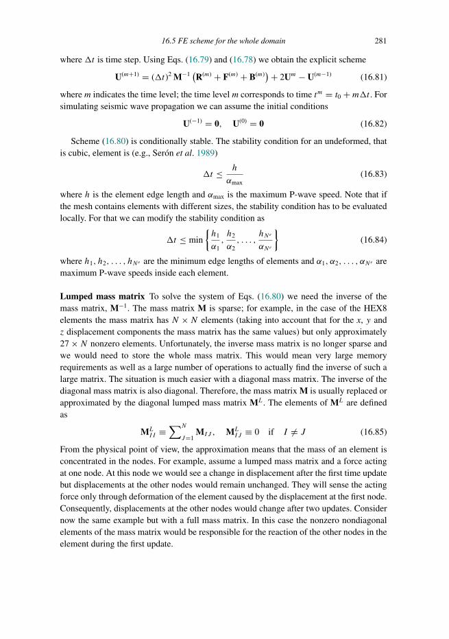
Trim: 247mm × 174mm Top: 14.762mm Gutter: 23.198mmCUUK2497-16 CUUK2497/Moczo ISBN: 978 1 107 02881 4 November 18, 2013 18:59
16.5 FE scheme for the whole domain 281
where �t is time step. Using Eqs. (16.79) and (16.78) we obtain the explicit scheme
U(m+1) = (�t)2 M−1(R(m) + F(m) + B(m))+ 2Um − U(m−1) (16.81)
where m indicates the time level; the time level m corresponds to time tm = t0 +m�t . Forsimulating seismic wave propagation we can assume the initial conditions
U(−1) = 0, U(0) = 0 (16.82)
Scheme (16.80) is conditionally stable. The stability condition for an undeformed, thatis cubic, element is (e.g., Seron et al. 1989)
�t ≤ h
αmax(16.83)
where h is the element edge length and αmax is the maximum P-wave speed. Note that ifthe mesh contains elements with different sizes, the stability condition has to be evaluatedlocally. For that we can modify the stability condition as
�t ≤ min
{h1
α1,h2
α2, . . . ,
hNe
αNe
}(16.84)
where h1, h2, . . . , hNe are the minimum edge lengths of elements and α1, α2, . . . , αNe aremaximum P-wave speeds inside each element.
Lumped mass matrix To solve the system of Eqs. (16.80) we need the inverse of themass matrix, M−1. The mass matrix M is sparse; for example, in the case of the HEX8elements the mass matrix has N ×N elements (taking into account that for the x, y andz displacement components the mass matrix has the same values) but only approximately27 ×N nonzero elements. Unfortunately, the inverse mass matrix is no longer sparse andwe would need to store the whole mass matrix. This would mean very large memoryrequirements as well as a large number of operations to actually find the inverse of such alarge matrix. The situation is much easier with a diagonal mass matrix. The inverse of thediagonal mass matrix is also diagonal. Therefore, the mass matrix M is usually replaced orapproximated by the diagonal lumped mass matrix ML. The elements of ML are definedas
MLII ≡
∑N
J=1MIJ , ML
IJ ≡ 0 if I = J (16.85)
From the physical point of view, the approximation means that the mass of an element isconcentrated in the nodes. For example, assume a lumped mass matrix and a force actingat one node. At this node we would see a change in displacement after the first time updatebut displacements at the other nodes would remain unchanged. They will sense the actingforce only through deformation of the element caused by the displacement at the first node.Consequently, displacements at the other nodes would change after two updates. Considernow the same example but with a full mass matrix. In this case the nonzero nondiagonalelements of the mass matrix would be responsible for the reaction of the other nodes in theelement during the first update.

Trim: 247mm × 174mm Top: 14.762mm Gutter: 23.198mmCUUK2497-16 CUUK2497/Moczo ISBN: 978 1 107 02881 4 November 18, 2013 18:59
282 Finite-element method
Even though the lumped mass matrix seems to change the physics dramatically, in manypractical applications the approach usually works well. However, there are situations whenit is not so – see Chapter 17 for an example.
16.6 Efficient computation of the restoring-force vector
To minimize the computational requirements one can use special coordinates for updatingthe restoring-force vector proposed by Balazovjech and Halada (2006) and Moczo et al.(2007a) for a 2D quadrilateral element. The description of an element in the standardcoordinates (local or physical) also contains information about the position/location of theelement. But the position/location is not needed for computation of the restoring force,because the restoring force depends only on the deformation of the element. ThereforeBalazovjech and Halada proposed parameterizing the element using new local coordinates.They called them e-invariants. The benefit of using e-invariants comes from the fact that theshape functions expressed in these local coordinates have a very simple form. Consequently,the number of operations required to update the restoring force is significantly lower thanin the case of the standard shape functions.
Here we show and briefly comment on the final expressions of the approach for therestoring-force computation in 3D (Balazovjech, personal communication). Recall thedefinition of the local restoring-force vector, Eq. (16.54). Consider only the element withoutnodes at boundary �D . In such a case sw = s and we can write
rx ≡∫�m
(s,x σxx + s,y σxy + s,z σxz
)det J d� (16.86)
We can do so analogously also for the y- and z-components.Define a transformation matrix:
T ≡
⎛⎜⎜⎜⎜⎜⎜⎜⎜⎜⎜⎜⎜⎜⎜⎜⎜⎜⎜⎝
1 1 1 1 1 1 1 1
−1 1 1 −1 −1 1 1 −1
−1 −1 1 1 −1 −1 1 1
−1 −1 −1 −1 1 1 1 1
1 −1 1 −1 1 −1 1 −1
1 1 −1 −1 −1 −1 1 1
1 −1 −1 1 −1 1 1 −1
−1 1 −1 1 1 −1 1 −1
⎞⎟⎟⎟⎟⎟⎟⎟⎟⎟⎟⎟⎟⎟⎟⎟⎟⎟⎟⎠
(16.87)
The shape functions for the reference element can be then expressed using matrix T:
s(inv) ≡ T s = (1, ξ, η, ζ, ξη, ηζ, ξζ, ξηζ )T (16.88)
Trim: 247mm × 174mm Top: 14.762mm Gutter: 23.198mmCUUK2497-16 CUUK2497/Moczo ISBN: 978 1 107 02881 4 November 18, 2013 18:59
16.7 Comparison of restoring force and stiffness matrix 283
(compare with the standard shape functions defined by Eq. (16.37)). Matrix T has theproperty
I = 18 TTT (16.89)
where I is the unit matrix.To compute the stresses needed in Eq. (16.85) we need to know the spatial derivatives
of displacement. Using (16.88) we express the spatial derivatives of displacement:
uei ,j = s,Tj · uei = s,Tj · ( 18 TTT
) · uei = 18 s,(inv)T
j · u(inv)i (16.90)
Using (16.88) we can rewrite the restoring force (16.85) in this form:
rx ≡ 18 TT
∫�m
(s(inv),x σxx + s(inv),y σxy + s(inv),z σxz
)det Jd� (16.91)
We can obtain the Jacobian for Eq. (16.90) from definition (16.40). We just have toreplace the expressions for coordinates x, y, z. We can express the physical coordinatesfrom Eq. (16.38) using the approach indicated in Eq. (16.89). We obtain
x = 18 s(inv)Tx(inv), y = 1
8 s(inv)Ty(inv), z = 18 s(inv)Tz(inv) (16.92)
where
x(inv) = T
⎛⎜⎜⎜⎝x1
x2...xn
⎞⎟⎟⎟⎠ , y(inv) = T
⎛⎜⎜⎜⎝y1
y2...yn
⎞⎟⎟⎟⎠ , z(inv) = T
⎛⎜⎜⎜⎝z1
z2...zn
⎞⎟⎟⎟⎠ (16.93)
16.7 Comparison of formulations with the restoring force and stiffness matrix
Compare the formulation with the restoring force (the one we use) with a common formu-lation based on the stiffness matrix K. The relation between the stiffness matrix and therestoring force may be written as
R = −K U (16.94)
Matrix K is very sparse. Consider a mesh of the HEX8 elements. The total number ofelements in the matrix K is 3N × 3N whereas the number of the nonzero elements isapproximately 3N × 81. Storing only the nonzero elements clearly is more feasible thanstoring all elements. However, considering the tens of millions of nodes in relatively modest3D numerical modelling, we easily realize that even the latter number of nonzero elementsposes a serious problem. The restoring-force vector has only 3N elements – we need tostore 81 times fewer elements compared to storing the nonzero elements in the stiffnessmatrix.
On the other hand, the stiffness matrix does not change with time – it is enough tocalculate it once at the beginning of simulation. The restoring force has to be updated

Trim: 247mm × 174mm Top: 14.762mm Gutter: 23.198mmCUUK2497-16 CUUK2497/Moczo ISBN: 978 1 107 02881 4 November 18, 2013 18:59
284 Finite-element method
at each time level. This means that the restoring force reduces memory requirements butincreases the number of algebraic operations.
Note that the stiffness matrix is time independent only if material parameters aretime independent. Nonlinear (e.g., elastoplastic) behaviour of a medium implies a time-dependent stiffness matrix. The matrix has to be updated at each time level and the stiffness-matrix formulation means both large memory and computational time requirements.
16.8 Essential summary of the FEM implementation
Use of the restoring-force concept significantly reduces the memory requirements comparedto the commonly used global stiffness matrix. The need to calculate the restoring forces ateach time level, however, increases the number of operations and thus the computationaltime. This increase can be significantly reduced by the use of e-invariants. Consequently,the combination of the restoring forces and e-invariants represents a memory-efficientimplementation of the FEM.
Trim: 247mm × 174mm Top: 14.762mm Gutter: 23.198mmCUUK2497-17 CUUK2497/Moczo ISBN: 978 1 107 02881 4 November 18, 2013 19:40
17
Traction-at-split-node modelling of dynamicrupture propagation
This chapter is devoted to implementation of the TSN method for modelling dynamicrupture propagation in the FE algorithm. There are different implementations of dynamicmodels in the FEM. Archuleta (1976) and Archuleta and Frazier (1978) published oneof the first implementations. Their rupture propagation was not spontaneous because therupture speed was prescribed but the evolution of traction was calculated. Day (1977)implemented his version of the TSN in the standard FE algorithm. Later Andrews (1999)implemented his version of the TSN in the FD algorithm with spatial differentiation equiv-alent to the FEM. The method was, however, limited to a homogeneous medium and ‘brick’elements. Oglesby (1999) implemented an algorithm for spontaneous rupture propagationinto Dyna2D (Whirley et al. 1992) and Dyna3D (Whirley and Engelmann 1993) codes.Because of the nature of the codes, Oglesby’s approach was based on elastic and frictionalforces. But, in fact, it was equivalent to Andrews’ version of the TSN.
17.1 Implementation of TSN in the FEM
Here we explain the TSN implementation in the FEM described in Chapter 14. We recallthat the TSN explained in Chapter 14 may be used with numerical methods with an explicittime-stepping algorithm and if the force applied at one node accelerates only that nodeduring one time iteration. These requirements are satisfied with the explicit scheme (16.80)with the lumped mass matrix (16.84). As we explained in Chapter 16, we use the lumpedmass matrix for practical reasons.
In a TSN the fault surface is covered by split nodes whereas the rest of the domain iscovered by normal nodes. Recall that a split node consists of two partial nodes – p.n.+
and p.n.−. The partial node p.n.+ belongs only to halfspace H+ whereas p.n.− belongsonly to halfspace H−. A partial node is characterized by quantities related to the relevanthalfspace (e.g., seismic wave speeds, density, displacements, particle velocities or forces). Acouple of the partial nodes share the fault-related quantities (e.g., slip, slip rate, coefficientsof friction). This imposes additional constraints in creating the global system of the FEequations from the local ones. We have to ensure that the restoring force at the partial nodep.n.− is only due to deformation in halfspace H− and, similarly, the restoring force at thepartial node p.n.+ is only due to deformation of the halfspace H+. Analogously, we have
285

Trim: 247mm × 174mm Top: 14.762mm Gutter: 23.198mmCUUK2497-17 CUUK2497/Moczo ISBN: 978 1 107 02881 4 November 18, 2013 19:40
286 TSN modelling of dynamic rupture propagation
to ensure that mass M− is only due to the density distribution in halfspace H− and massM+ is only due to the density distribution in halfspace H+. In other words, if there is nointeraction between the partial nodes p.n.+ and p.n.−, the partial nodes should behave asnodes at a free surface.
The first step in the TSN algorithm is to compute the trial traction �T ct . RecallEq. (14.11):
�T ct (t) ≈ �T 0 +M−M+
�t�s(t − �t
2
)+M− �F+(t) −M+ �F−(t)
A (M− +M+)(17.1)
Forces �F+ and �F− are components of the global restoring-force vector corresponding tothe partial nodes p.n.+ and p.n.−, respectively.
Vector �T ct can be decomposed into the normal and shear (tangential) components:
�T ctn (t) = [ �T ct (t).�n]�n�T ctsh (t) = �T ct (t) − �T ctn (t)
(17.2)
To evaluate the fault strength S(t) according to the linear slip-weakening friction law (4.11),we need the slip path l defined by (4.10). The slip path at time t can be approximated:
l(t) = l(t −�t) +�t |�s(t −�t/2)| (17.3)
The total traction on the fault, �T c(t), and the slip rate are determined by Eqs. (14.12),(14.22) and (14.16):∣∣ �T ctsh (t)
∣∣ ≤ S(t): �T c(t) = �T ct (t) ⇒ �s (t + 12�t
) = 0∣∣ �T ctsh (t)∣∣ > S(t): �T cn (t) = �T ctn (t) ⇒ �sn
(t + 1
2�t) = 0
�T csh(t) = S(t)�T ctsh (t)∣∣ �T ctsh (t)
∣∣ ⇒ �ssh(t + 1
2�t) ≈ �t B[ �T ctsh (t) − �T fsh(t)
](17.4)
The updated slip-rate value is then used to obtain the displacements at the partial nodesp.n.+ and p.n.−. The velocity of the centroid of two partial nodes is
�vcent(t + 1
2�t) = �vcent
(t − 1
2�t)+�t
�F+(t) + �F−(t)
M+ +M− (17.5)
The slip rate, that is, the differential velocity between two partial nodes, is distributedbetween the partial nodes according to their masses:
�v− (t + 12�t
) = �vcent(t + 1
2�t)−�tM
+�s (t + 12�t
)M+ +M− (17.6)
�v+ (t + 12�t
) = �vcent(t + 1
2�t)+�tM
−�s (t + 12�t
)M+ +M− (17.7)

Trim: 247mm × 174mm Top: 14.762mm Gutter: 23.198mmCUUK2497-17 CUUK2497/Moczo ISBN: 978 1 107 02881 4 November 18, 2013 19:40
17.1 Implementation of TSN in the FEM 287
The displacements at the partial nodes are then
�u−(t +�t) = �u−(t) +�t �v−(t + 12�t) (17.8)
�u+(t +�t) = �u+(t) +�t �v+(t + 12�t) (17.9)
The problem with integration: why the 8-point Gaussian integration does not workAs we explained in Chapter 16, numerical integration is used to compute the restoring-force vector or mass matrix. Because of its accuracy and efficiency, the 8-point Gaussianintegration is usually used with the HEX8 element with trilinear shape functions. We alsorecall that for practical reasons the lumped mass matrix, Eq. (16.84), is usually used insteadof the fully integrated mass matrix. However, our numerical tests showed that 8-pointGaussian integration does not produce the correct solution for rupture propagation with theTSN implementation. To explain this behaviour we have to look at the integration in detail.
A nondiagonal mass matrix is a consequence of the properties of the shape functionsand locations of integration points. The integration points for 8-point Gaussian integrationare located inside an element where all shape functions are nonzero. Therefore, matrixme, Eq. (16.48), consists of only nonzero elements and consequently the mass matrix isnondiagonal.
As we briefly mentioned in Chapter 16, we can use other integration schemes. For someapplications it may be advantageous to use schemes with lower-order accuracy than whatis required, also known as reduced integration. Sometimes, however, reduced integrationmay lead to solutions polluted by oscillations (also known as hourglass modes, zero-energymodes or spurious zero-energy modes). If the solution is not affected by the oscillations,it may be considered a reasonable solution (e.g., Ottosen and Petersson 1992, Zienkiewiczand Taylor 1989).
We can use, for example, the 8-point Lobatto integration. This integration is accurateonly for linear functions (compare with the accuracy of 8-point Gaussian integration). Theintegration points for 8-point Lobatto integration are located at nodes, where always oneshape function equals 1 and all others equal 0. Therefore, the mass matrix computed by 8-point Lobatto integration is naturally diagonal. Moreover, it can be shown that it is the sameas the lumped mass matrix. Our numerical tests showed that 8-point Lobatto integrationproduces a solution close to the reference solution even for rupture propagation with theTSN implementation.
The use of 8-point Gauss integration with the lumped mass matrix is the equivalent ofusing 8-point Lobatto integration to compute the mass matrix and using 8-point Gaussianintegration to compute the restoring force. Therefore, we conjecture that the combinationof different integration schemes used for integrating the mass matrix and restoring force isthe reason why 8-point Gaussian integration does not produce the correct solution with theTSN implementation.
Intuitively we can expect that the integration scheme may affect the stability of thefinal scheme. The stability of the HEX8 elements with reduced integration was analyzedby Hughes (2000), who refers to Flanagan and Belytschko (1981). For a ‘brick’ element
Trim: 247mm × 174mm Top: 14.762mm Gutter: 23.198mmCUUK2497-17 CUUK2497/Moczo ISBN: 978 1 107 02881 4 November 18, 2013 19:40
288 TSN modelling of dynamic rupture propagation
with size hx in the x-direction, hy in the y-direction and hz in the z-direction the stabilitycondition is
�t ≤(αmax
√h−2x + h−2
y + h−2z
)−1
(17.10)
For a cube element with h = hx = hy = hz the condition simplifies:
�t ≤ h√3αmax
(17.11)
Comparing Eqs. (17.11) and (16.82) we see that the time step is smaller if reduced integra-tion is applied.
For completeness, we should explain why 8-point Gaussian integration with the lumpedmass matrix works for kinematic sources. In our approach, the kinematic point sourceis implemented using body forces. Our numerical tests showed that 8-point Gaussianintegration with the lumped mass matrix produces large errors and opposite polarization atthe nodes next to nodes at which the force is applied. This error is spatially very localizedand strongly vanishes with distance. Moreover, the kinematic sources have time evolutionprescribed a priori and therefore this localized error does not affect the source. In the case ofthe dynamic model the error appears in the neighbourhood of the partial node and reaches itsmaximum value at nodes next to the partial node. Therefore, the deformation of halfspacesand consequently also computation of forces �F+ and �F− is affected. In the case of thedynamic model the interaction between the radiated wavefield and rupture propagation iscrucial. Therefore, the error affects the evolution of the rupture. Consequently, the radiatedwavefield is also affected and the error is no longer local.
17.2 Spurious high-frequency oscillations of the slip rate
Despite the superior properties of the TSN method, the slip-rate time histories obtained usingthe TSN very often contain spurious high-frequency oscillations. We briefly summarizepossible reasons leading to these oscillations following Galis et al. (2010).
For a given initial stress and material parameters on a fault, it is the friction law thatcontrols initialization, propagation and healing of rupture. First, consider Coulomb friction;that is, a very simple friction law with an instantaneous change of traction from the yieldto the dynamic value (Fig. 17.1a). The stress is discontinuous at the crack tip. This impliesan infinitely large slip rate at the crack tip. The slip-rate value then rapidly decreases withtime. The narrow pulse of the slip rate with infinite peak value implies an infinitely broadspectrum and thus also very high frequencies.
Next, consider a linear slip-weakening friction law (Fig. 17.1b). The gradual decreaseof stress (during finite time and slip) removes the infinite value of the slip rate at the cracktip. Naturally, the steeper is the decrease of the stress in the friction law, the steeper is theincrease of the slip rate and, consequently, the broader is the spectrum of the shear-stressand slip-rate variations generated by the slipping point. The spectrum of the slip rate is

Trim: 247mm × 174mm Top: 14.762mm Gutter: 23.198mmCUUK2497-17 CUUK2497/Moczo ISBN: 978 1 107 02881 4 November 18, 2013 19:40
17.2 Spurious high-frequency oscillations of the slip rate 289
slip
(a) Coulomb friction law (b) Linear slip-weakening
friction law
slipcD
0τ
sτ
dτfrict
iona
l tra
ctio
n
dτ
sτ
0τ
Figure 17.1 Coulomb friction law (a) and linear slip-weakening friction law (b). Here τ0 is initialtraction, τs static traction and τd dynamic traction.
discussed also by Kaneko et al. (2008) and de la Puente et al. (2009). Note that in thelimiting case of an infinite slope the slip-weakening friction law becomes the Coulombfriction law.
The gradual decrease of the stress at a slipping point implies the existence of a breakdownzone – the spatial zone on the fault plane behind the crack tip where the shear stress decreasesfrom its static to its dynamic value.
Thus, a possibly broad-spectrum slip-rate and stress variations generated by each slippingpoint as well as the spatial breakdown zone have to be properly discretized in a numericalmethod in order to avoid the effect of numerical grid dispersion at higher frequencies andto properly capture the stress changes in the breakdown zone.
The wave propagation problems are linear. Therefore, it is relatively easy to correctlytreat high frequencies in the discrete model. The effect of numerical grid dispersion maybecome considerable/visible for wavelengths sampled by less than a certain number ofsamples. Therefore, the size of the spatial grid spacing determines how accurately highfrequencies are propagated by a grid. Moreover, because of the linear character of thewave propagation problem, it is possible to apply a-posteriori filtration to remove the highfrequencies as long as the high-frequency content did not affect (due to the accuracy ofnumber representation or not-a-number values) the content at lower frequencies.
In the rupture propagation problems, the effect of numerical grid dispersion may becomemore dramatic due to nonlinear coupling between the shear stress and slip rate. In the TSNmethod a slip-rate increment at each time level is calculated from the difference betweenthe trial traction �T ct and frictional traction at a point of the fault, Eq. (17.4). Whereas thefrictional traction itself does not suffer from oscillations (because it is determined by thefriction law), �T ct is not smooth in time, reflecting the presence of high-frequency stressvariations inaccurately propagated by the grid. The inaccurately determined slip-rate incre-ment is used in calculation of the slip rate in the next time level – thus causing oscillationsof the slip rate, which in turn affects the value of the trial traction.
Trim: 247mm × 174mm Top: 14.762mm Gutter: 23.198mmCUUK2497-17 CUUK2497/Moczo ISBN: 978 1 107 02881 4 November 18, 2013 19:40
290 TSN modelling of dynamic rupture propagation
Thus, for a given friction law (for a given steepness of the stress decrease) and orderof approximation in the applied numerical method, it is the size of the spatial grid spacingthat determines how accurately high frequencies are propagated by the grid and how largeare the high-frequency oscillations of the slip rate. In most practical applications the spatialsampling will probably not be fine enough to prevent visible spurious oscillations in thelow-order approximation numerical method.
If the high-frequency content does not affect the development and propagation of rupture,it is possible to apply a-posteriori filtration to remove the oscillations. However, becauseof the nonlinear character of rupture propagation we cannot, in general, a-priori assumethat the high-frequency content would not change the development and propagation ofrupture. Therefore, a-posteriori filtration cannot serve as a systematic tool for reducing theoscillations. If the high frequencies affect rupture propagation, then the only possibilityis to utilize run-time methods to suppress the high-frequency oscillations. In the nextsection we discuss three different methods to suppress the oscillations, including a-posteriorifiltration.
17.3 Approaches to suppress high-frequency oscillations
17.3.1 Adaptive smoothing
In this section we present an adaptive smoothing algorithm for suppressing/reducing spu-rious high-frequency oscillations of the slip-rate time histories in the FE–TSN modellingof dynamic rupture with slip-dependent friction laws proposed by Galis et al. (2010).
As outlined in Section 17.2, in the TSN method a slip-rate increment at each time level iscalculated from the difference between the trial traction �T ct and frictional traction. The trialtraction is not smooth due to the high-frequency stress variations inaccurately propagatedby the grid. To suppress or reduce these oscillations we can spatially smooth �T ct . There aredifferent ways to spatially smooth �T ct . In the algorithm proposed by Galis et al. (2010) itis possible to control when and how to apply smoothing.
If the smoothing is applied to the entire fault it removes high frequencies also from therupture front. Consequently, it affects rupture propagation. Therefore, we should apply thesmoothing only behind the rupture front. Then the question is, how to identify the rupturefront. The best results were obtained with the so-called 9-point threshold criterion, that is,the smoothing is applied when the slip rate is larger than 0 m/s simultaneously at a nodeand at eight neighboring nodes (assuming a regular mesh of the HEX8 elements).
Once the threshold criterion for the application of smoothing is satisfied, we applythe smoothing. The smoothing is defined as a weighted average of the original �T ct andGaussian-filtered �T ct . Let p be the averaging parameter and 0 ≤ p ≤ 1. Assume a regularmesh of nodes on the fault plane such that we can refer to the nodes on the fault plane usingindices (i, j ). Then the smoothed traction at point (i, j ) can be defined as
�T ct (i, j ) ≡∑i+1
k=i−1
∑j+1
l=j−1wkl �T ct (k, l) (17.12)

Trim: 247mm × 174mm Top: 14.762mm Gutter: 23.198mmCUUK2497-17 CUUK2497/Moczo ISBN: 978 1 107 02881 4 November 18, 2013 19:40
17.3 Approaches to suppress high-frequency oscillations 291
314
p−
8
p
16
p
8
p
8
p
8
p
16
p
16
p
16
p
1j −
j
1j +
1i − i 1i +
Figure 17.2 Scheme of the effective weighting coefficients in the adaptive smoothing algorithm forcalculation of the trial traction at grid position (i, j) on the fault plane. The averaging parameterp ∈ 〈0, 1〉 and may vary with time. (Modified from Galis et al. 2010)
where
w ≡⎛⎝p/16 p/8 p/16p/8 1 − 3p/4 p/8p/16 p/8 p/16
⎞⎠ (17.13)
Note that for p = 0 and p = 1 the matrix of the weight coefficients w becomes
w0 =⎛⎝0 0 0
0 1 00 0 0
⎞⎠ , w1 =
⎛⎝1/16 1/8 1/16
1/8 1/4 1/81/16 1/8 1/16
⎞⎠ (17.14)
respectively. Also note that w1 is identical to the coefficients of the Gaussian filter. Thesmoothing is illustrated in Fig. 17.2.
The values of the parameters were calibrated using extensive numerical tests. One of thekey requirements was the minimal impact of the smoothing on rupture propagation speed.The other key requirement was, naturally, the efficiency in suppressing high-frequencyoscillations. The numerical tests showed that better results were obtained when smoothingwas applied gradually behind the rupture front. In looking for the smoothing algorithmand values of parameters we chose a configuration with sub-Rayleigh rupture speed andone discretization. Afterwards, we tested the best algorithm and parameters also for otherdiscretizations and a configuration with super-shear rupture propagation speeds.
Based on the performed numerical tests, we define adaptive smoothing as follows: pvaries linearly from 0 for no slip to pmax = 0.4 when slip reaches the critical distance. Forlarger slip p remains constant. The numerical tests demonstrated that adaptive smoothingis capable of significantly reducing high-frequency oscillations without affecting rupturepropagation speed. Adaptive smoothing is illustrated in Fig. 17.3.
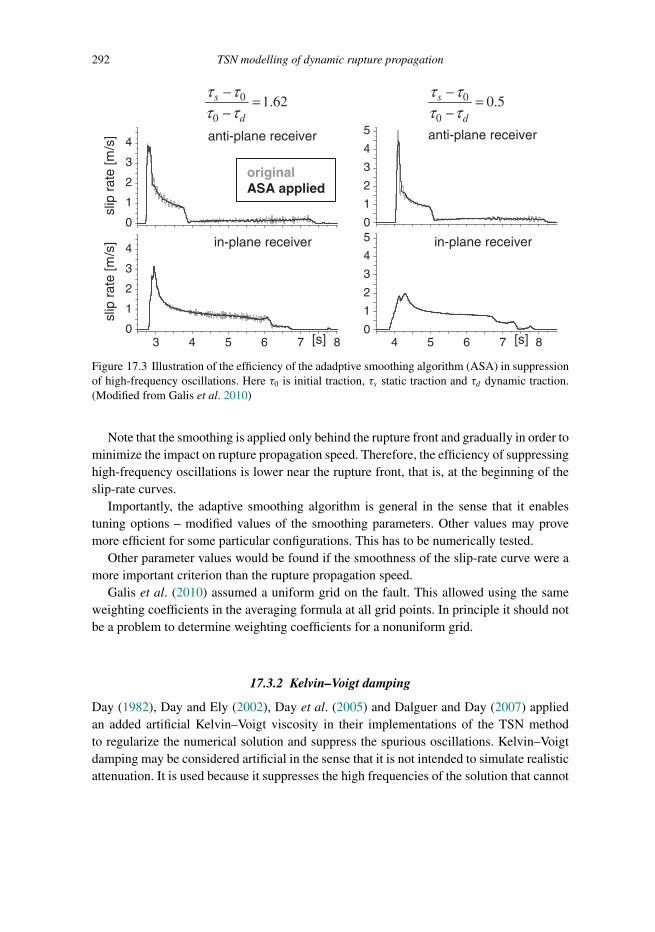
Trim: 247mm × 174mm Top: 14.762mm Gutter: 23.198mmCUUK2497-17 CUUK2497/Moczo ISBN: 978 1 107 02881 4 November 18, 2013 19:40
292 TSN modelling of dynamic rupture propagation
4
3
2
1
04 5 6 7 8[s]
4
3
2
1
0
5
0
01.62s
d
τ ττ τ
−=
−0
00.5s
d
τ ττ τ
−=
−
4
3
2
1
0
54
3
2
1
0
[s]
slip
rat
e [m
/s]
slip
rat
e [m
/s]
anti-plane receiver
in-plane receiver
4 5 6 73 8
anti-plane receiver
in-plane receiver
originalASA applied
Figure 17.3 Illustration of the efficiency of the adadptive smoothing algorithm (ASA) in suppressionof high-frequency oscillations. Here τ0 is initial traction, τs static traction and τd dynamic traction.(Modified from Galis et al. 2010)
Note that the smoothing is applied only behind the rupture front and gradually in order tominimize the impact on rupture propagation speed. Therefore, the efficiency of suppressinghigh-frequency oscillations is lower near the rupture front, that is, at the beginning of theslip-rate curves.
Importantly, the adaptive smoothing algorithm is general in the sense that it enablestuning options – modified values of the smoothing parameters. Other values may provemore efficient for some particular configurations. This has to be numerically tested.
Other parameter values would be found if the smoothness of the slip-rate curve were amore important criterion than the rupture propagation speed.
Galis et al. (2010) assumed a uniform grid on the fault. This allowed using the sameweighting coefficients in the averaging formula at all grid points. In principle it should notbe a problem to determine weighting coefficients for a nonuniform grid.
17.3.2 Kelvin–Voigt damping
Day (1982), Day and Ely (2002), Day et al. (2005) and Dalguer and Day (2007) appliedan added artificial Kelvin–Voigt viscosity in their implementations of the TSN methodto regularize the numerical solution and suppress the spurious oscillations. Kelvin–Voigtdamping may be considered artificial in the sense that it is not intended to simulate realisticattenuation. It is used because it suppresses the high frequencies of the solution that cannot

Trim: 247mm × 174mm Top: 14.762mm Gutter: 23.198mmCUUK2497-17 CUUK2497/Moczo ISBN: 978 1 107 02881 4 November 18, 2013 19:40
17.3 Approaches to suppress high-frequency oscillations 293
be accurately computed by the grid. For implementing Kelvin–Voigt damping, Day and hiscolleagues considered the stress–strain relation in the form
σij = λ∂uk∂xkδij + μ
(∂ui
∂xj+ ∂uj∂xi
)+ η�t
[λ∂uk
∂xkδij + μ
(∂ui
∂xj+ ∂uj∂xi
)](17.15)
where η is a damping parameter and u is the particle velocity. Day (1982), Day and Ely(2002) and Day et al. (2005) applied Kelvin–Voigt damping in the DFM (discrete faultmodel) implementation of TSN, that is, in their FD scheme on the partly staggered grid.This scheme suffers from the so-called hourglass modes (zero-energy modes). Kelvin–Voigt damping helps in suppressing these modes. Therefore, the damping was applied inthe whole grid. For this approach a preferred value of damping is η ∼ 0.1 (Day et al. 2005).Dalguer and Day (2007) applied Kelvin–Voigt damping in their SGSN method (staggered-grid split-node FD implementation of TSN). The staggered-grid FD scheme does not sufferfrom hourglass modes. Therefore, artificial damping was applied only to the fault surfaceto suppress spurious high-frequency oscillations. The corresponding damping parameterηs is therefore not equivalent to parameter η. Dalguer and Day numerically examinedthe sensitivity of the solution with respect to ηs . They found that although their methodconverges even with no artificial damping applied, the application of damping with propervalues of ηs greatly accelerates the convergence. Artificial damping reduces the rupturetime error and spurious oscillations in the slip-rate time histories if a proper value of thedamping parameter is used. However, the peak slip-rate misfit increases with damping(having a minimum if no damping is applied). They concluded that the preferred value ofthe damping parameter is ηs ∼ 0.3, but the optimal value is likely problem dependent.
17.3.3 A-posteriori filtration
If spurious high-frequency oscillations appeared in numerical simulations of rupture prop-agation, were not sufficiently reduced or suppressed by artificial damping or adaptivesmoothing, and did not unphysically affect development and propagation of rupture, itis possible and reasonable to apply a-posteriori filtration to the simulated slip-rate timehistories. Kristekova et al. (2012) quantitatively compared three methods of a-posteriorifiltration – low-pass filtering, discrete-wavelet denoising, empirical-mode-decompositiondenoising – and adaptive smoothing. They used a set of slip-rate time histories simulatedby the 3D FEM–TSN on a planar fault. The simulated slip-rate histories were obtainedwith a cubic mesh and four discretizations (25 m, 50 m, 100 m and 150 m); see Galis et al.(2010). The smooth reference slip-rate time history was obtained by a careful iterativeand adjusted denoising of the slip-rate simulated using the finest (technically possible)discretization (25 m). The efficiency of the smoothing methods was evaluated using time–frequency analysis and time–frequency misfit criteria (Kristekova et al. 2006, 2009) basedon the continuous wavelet transform. The time–frequency tools were capable of clearlyindicating distortions caused by spurious oscillations and/or by a-posteriori filtration.

Trim: 247mm × 174mm Top: 14.762mm Gutter: 23.198mmCUUK2497-17 CUUK2497/Moczo ISBN: 978 1 107 02881 4 November 18, 2013 19:40
294 TSN modelling of dynamic rupture propagation
The main conclusion of the investigation by Kristekova et al. (2012) is that the safestway to reduce/suppress the oscillations is to apply a method that reduces the oscillationsduring numerical simulation of rupture propagation, e.g., adaptive smoothing. The adaptivesmoothing algorithm does not distort the slip-rate and considerably reduces oscillations.Slight oscillations can remain in the tail. They can be safely removed a posteriori ifnecessary.
The result of application of low-pass filtering is very sensitive to the choice of cornerfrequency. Determination of the optimal corner frequency can be problematic even usingthe Fourier spectrum of the slip-rate time history. It is considerably better to determineit using the time–frequency representation of the slip-rate history. A proper filter shouldbe selected for each slip-rate history separately, taking into account the character of boththe slip-rate history and oscillations. Application of the same filter to many different slip-rate time histories can lead to considerable distortions of some of them. Considering allthe mentioned aspects, low-pass filtering can give good results but only with carefullydetermined parameters of the filter.
Discrete-wavelet denoising (e.g., Donoho 1995) can reduce spurious high-frequencyoscillations, but if the oscillations overlap with the main slip-rate peak the discrete-waveletdenoising is not as efficient as other methods in the vicinity of the peak and behind it.
Empirical-mode-decomposition denoising (e.g., Flandrin et al. 2004) is efficient andsufficiently accurate in the vicinity of the slip-rate peak. Some small oscillations canremain in the tail; if necessary it is easy to suppress them by additional filtering. Themain advantage of empirical-mode-decomposition denoising is that it is an adaptive data-driven method and therefore it can be applied automatically (in the simplest version evenwithout determining parameters of denoising). This property makes the method suitablefor processing large data sets of different slip-rate time histories.

Trim: 247mm × 174mm Top: 14.762mm Gutter: 23.198mmCUUK2497-18 CUUK2497/Moczo ISBN: 978 1 107 02881 4 November 18, 2013 19:22
18
Hybrid finite-difference–finite-element method
The FEM more easily incorporates boundary conditions at the free surface compared to theFDM. This is true for a planar free surface as well as for free-surface topography. Therefore,the FEM is better suited for simulating the traction-free condition and rupture propagationthan the FDM. On the other hand, an FD scheme can computationally be considerablymore efficient for modelling seismic wave propagation, for instance, if the seismic wavesproduced by a dynamically rupturing fault are to be propagated away from the fault. It istherefore natural to think of a hybrid combination of the two methods if we want to includeboth a dynamic earthquake source and wave propagation in a complex heterogeneousmedium. Moczo et al. (1997) combined the (2,2) conventional displacement FD schemewith the (2,2) standard FE scheme for 2D viscoelastic P-SV modelling of seismic motionin near-surface sedimentary/topographic structures. Ma et al. (2004) combined the (2,4)velocity–stress staggered-grid (VS SG) scheme with the (2,2) standard FE scheme for 2Delastic P-SV modelling.
In this chapter we explain the hybrid method developed by Galis et al. (2008). Thishybrid method combines the (2,2) standard FE scheme with the (2,4) VS SG scheme for3D viscoelastic modelling.
18.1 Computational domain
As already pointed out, the main idea of the hybrid combination of the two methods isto achieve efficient numerical simulations for important realistic problem configurations.Such configurations may include free-surface topography and material heterogeneity aswell as a dynamically rupturing fault. Correspondingly, a computational domain of thehybrid FD–FE method may include one or more FE regions that would cover those parts ofthe model where the free-surface topography or fault has to be considered. To achieve betterefficiency, the FE regions should be as small as possible compared to the FD region, whichshould cover a major part of the whole computational domain. The computational domain isschematically illustrated in Fig. 18.1. It is crucial that the FE regions causally communicateat each time level with the FD region. The FD–FE communication is explained in detail inthe following sections.
295

Trim: 247mm × 174mm Top: 14.762mm Gutter: 23.198mmCUUK2497-18 CUUK2497/Moczo ISBN: 978 1 107 02881 4 November 18, 2013 19:22
296 Hybrid FD–FE method
FE Region
FD Region
Fault plane
Figure 18.1 Illustration of the computational domain. The FE region can cover the part of the modelwith free-surface topography (left) or a dynamically rupturing surface (right). The rest of the domainis covered with the FD grid. One computational domain can, in principle, include several FE regions.
18.2 Principle of the FD–FE causal communication
At each time level: (1) the wavefields in the FE region(s) and FD regions are updatedindependently by the FE and FD schemes, respectively; (2) the FE region(s) and FD regioncausally communicate (exchange appropriate values) within the FD–FE transition zone.Given the structures of both schemes, the transition zone has to consist of several grid(mesh) surfaces at which the FD and FE regions overlap.
In the FD–FE transition zone the size of the grid spacing in the FE grid is twice assmall as that in the FD grid. Away from the transition zone the size of an element can,in principle, vary. The twice-smaller FE grid spacing is algorithmically the most naturaloption because any other ratio between the FD and FE grid spacings would make theschemes for updating in the transition zone much more complicated and it is likely that itwould produce more numerical noise. Intuitively, at a rough estimate, such a choice seemsreasonable given the 2nd- and 4th-order approximations of spatial derivatives in the FE andFD schemes, respectively. Strictly speaking, however, the spatial sampling does not simplyscale with the approximation order. For example, an increase in the approximation orderby two does not mean that a twice-larger grid spacing can be used. This is additionallyand independently supported by results obtained by Kristek and Moczo (2006). Theyindicated by their numerical investigations for the 1D problem that the 4th-order staggered-grid scheme requires denser spatial sampling than that usually used by many users, whoconsider it approximately twice as coarse as that in the 2nd-order conventional schemes.This indicates that if we apply proper sampling in the FD region, the FE region should beover-sampled. But in many applications this will cause no problems, because the modellingof the free-surface topography or dynamic rupture propagation requires denser spatialsampling compared to that usually used for wave propagation.

Trim: 247mm × 174mm Top: 14.762mm Gutter: 23.198mmCUUK2497-18 CUUK2497/Moczo ISBN: 978 1 107 02881 4 November 18, 2013 19:22
18.3 Smooth transition zone with FD–FE averaging 297
updated using the FEM
FD Dirichlet zoneAveraging
zoneFE Dirichletboundary Transition zone
FD regionstaggered grid
UWzxT
, ,xx yy zzT T T UW }
FE region
hFD
hFE
Figure 18.2 Illustration of the FD–FE transition zone used in hybrid modelling for causal FD–FEcommunication at each time level. For simplicity, only one vertical grid plane is shown. hFD is thespatial grid spacing in the FD grid. hFE is the spatial grid spacing in the uniform part of the FE grid inand near the transition zone; the rest of the FE grid can be nonuniform. Note that no special symbolis used to indicate the positions of the displacement vector in the FE grid. Each intersection of thegrid lines in the FE region is a position of all the components of the displacement vector.
18.3 Smooth transition zone with FD–FE averaging
The shape and size of the transition zone are basically determined by the FD schemesfor updating the particle-velocity and stress-tensor components. The transition zone isillustrated in Fig. 18.2. The figure shows an example of a vertical cross-section of aparticular transition zone. The zone consists of the FE Dirichlet boundary, the FD–FEaveraging zone, and the FD Dirichlet zone. It is clear that the FE Dirichlet boundary forthe 2nd-order displacement FE scheme consists of a single staircase grid surface that has togo through the grid points of the FD staggered grid. At the same time, a finite-thicknessDirichlet zone is necessary for the 4th-order velocity–stress staggered-grid FD scheme.
Note that causal FD–FE communication is formally possible even without the averagingzone. However, our numerical tests (Galis et al. 2008) clearly show that the averagingzone significantly improves results – even a one-grid-spacing thick averaging zone makesa significant difference in the numerical behaviour of the transition zone.
The local thickness and staircase shape of the FD Dirichlet zone are determined bythe following requirement: the particle velocity at the FD grid points located at the gridinterface between the averaging zone and the FD Dirichlet zone should be calculated usingthe 4th-order velocity–stress staggered-grid FD scheme for an interior grid point. This ispossible if relevant stress-tensor components are available. The FD Dirichlet zone has toinclude those stress-tensor components. In principle, those stress-tensor components could
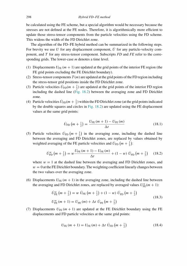
Trim: 247mm × 174mm Top: 14.762mm Gutter: 23.198mmCUUK2497-18 CUUK2497/Moczo ISBN: 978 1 107 02881 4 November 18, 2013 19:22
298 Hybrid FD–FE method
be calculated using the FE scheme, but a special algorithm would be necessary because thestresses are not defined at the FE nodes. Therefore, it is algorithmically more efficient toupdate those stress-tensor components from the particle velocities using the FD scheme.This widens the width of the FD Dirichlet zone.
The algorithm of the FD–FE hybrid method can be summarized in the following steps.For brevity we use U for any displacement component, U for any particle-velocity com-ponent, and T for any stress-tensor component. Subscripts FD and FE refer to the corre-sponding grids. The lower-case m denotes a time level.
(1) Displacements UFE (m+ 1) are updated at the grid points of the interior FE region (theFE grid points excluding the FE Dirichlet boundary).
(2) Stress-tensor componentsT (m) are updated at the grid points of the FD region includingthe stress-tensor grid positions inside the FD Dirichlet zone.
(3) Particle velocities UFD(m+ 12 ) are updated at the grid points of the interior FD region
including the dashed line (Fig. 18.2) between the averaging zone and FD Dirichletzone.
(4) Particle velocities UFD(m+ 12 ) within the FD Dirichlet zone (at the grid points indicated
by the double squares and circles in Fig. 18.2) are updated using the FE displacementvalues at the same grid points:
UFD(m+ 1
2
) = UFE (m+ 1) − UFE (m)
�t(18.1)
(5) Particle velocities UFD(m+ 1
2
)in the averaging zone, including the dashed line
between the averaging and FD Dirichlet zones, are replaced by values obtained byweighted averaging of the FE particle velocities and UFD
(m+ 1
2
):
UwFD
(m+ 1
2
) = wUFE (m+ 1) − UFE (m)
�t+ (1 − w) UFD
(m+ 1
2
)(18.2)
where w = 1 at the dashed line between the averaging and FD Dirichlet zones, andw = 0 at the FE Dirichlet boundary. The weighting coefficient linearly changes betweenthe two values over the averaging zone.
(6) Displacements UFE (m+ 1) in the averaging zone, including the dashed line betweenthe averaging and FD Dirichlet zones, are replaced by averaged values UwFE(m+ 1):
UwFE
(m+ 1
2
) = w UFE(m+ 1
2
)+ (1 − w) UFD
(m+ 1
2
)UwFE (m+ 1) = UFE (m) +�t UFE
(m+ 1
2
) (18.3)
(7) Displacements UFE (m+ 1) are updated at the FE Dirichlet boundary using the FEdisplacements and FD particle velocities at the same grid points:
UFE (m+ 1) = UFE (m) +�t UFD(m+ 1
2
)(18.4)

Trim: 247mm × 174mm Top: 14.762mm Gutter: 23.198mmCUUK2497-18 CUUK2497/Moczo ISBN: 978 1 107 02881 4 November 18, 2013 19:22
18.4 Illustrative numerical simulations 299
Recall that the FE Dirichlet boundary consists of a single staircase grid surface thatgoes through the grid points of the FD staggered grid. A grid position of the FD staggeredgrid is the position of either just one particle-velocity component or one shear stress-tensorcomponent or three normal stress-tensor components or no field variable. The symbolicEqs. (18.3) and (18.4) require all the particle-velocity components at a given grid position.Consequently, an interpolation of the missing particle-velocity components is necessary.We refer to Fig. 4 and Eqs. (33)–(41) in the article by Galis et al. (2008) for the possiblespatial configurations of the grid positions at which interpolations are necessary and theinterpolation formulas.
Galis et al. (2008) performed extensive numerical tests of the behaviour of the FD–FEtransition zone. They found no evidence of instabilities in practically sufficiently long timewindows. The averaging zone is crucial for accuracy. The FD–FE transition zone withoutthe averaging zone produces slight but evident numerical noise.
They also found that simulating dynamic rupture needs a sufficient distance (at leastnine FE grid spacings) between the FD–FE transition zone and the fault. For smallerdistances the FD–FE transition zone slightly affects the rupture propagation. The FD–FEtransition zone is stable and provides sufficiently accurate results also in the case of amaterial interface intersecting the transition zone.
Based on extensive numerical tests, Galis et al. (2008) concluded that the hybrid FD–FEmethod is stable, converging and sufficiently accurate.
18.4 Illustrative numerical simulations using hybrid FD–FE method
Galis et al. (2008) illustrated the hybrid FD–FE method by simulating two hypotheticalearthquakes near Grenoble, France. One was the thrust event beneath Grenoble, the otherwas a strike-slip event in the Belledonne Massif. They were inspired by a previous study byCotton et al. (1998), who considered point sources. Galis et al. (2008) used finite sourceswith dynamic rupture propagation with a linear-slip weakening friction law. A continuousincrease of the static and dynamic coefficients of friction was used to restrict rupture to anarea approximately 4 km × 2 km in order to produce an Mw = 5.3 event. The parametersinside this area were constant, except in the initiation zone. Even though both faults wereplanar, application of the hybrid method was advantageous due to the higher accuracy ofthe FEM for dynamic rupture propagation.
The structure of the sediment–bedrock interface together with the positions of the faultsfor both events is shown in Fig. 18.3. The horizontal fault is located at a depth of 5 km.The top of the vertical fault is at a depth of approximately 1.5 km and the ruptured areareaches a depth of approximately 3.5 km. The fault is located in the FE box and the restof the computational domain is covered by the FD grid. Because the FE box is relativelysmall in comparison to the size of the whole domain, the hybrid FD–FE simulations aresignificantly more efficient compared to simulations in which only the FE modelling isapplied to the whole domain. The simulations are accurate up to approximately 7.6 Hz inthe bedrock and up to approximately 0.7 Hz near the free surface in the sediments.
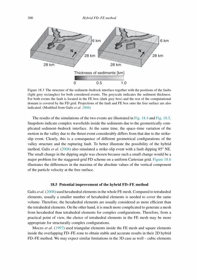
Trim: 247mm × 174mm Top: 14.762mm Gutter: 23.198mmCUUK2497-18 CUUK2497/Moczo ISBN: 978 1 107 02881 4 November 18, 2013 19:22
300 Hybrid FD–FE method
Thickness of sediments [km]
1.00.50
N
28 km
28 km
6 km
N
28 km
28 km
6 km
Figure 18.3 The structure of the sediment–bedrock interface together with the positions of the faults(light grey rectangles) for both considered events. The greyscale indicates the sediment thickness.For both events the fault is located in the FE box (dark grey box) and the rest of the computationaldomain is covered by the FD grid. Projections of the fault and FE box onto the free surface are alsoindicated. (Modified from Galis et al. 2008)
The results of the simulations of the two events are illustrated in Fig. 18.4 and Fig. 18.5.Snapshots indicate complex wavefields inside the sediments due to the geometrically com-plicated sediment–bedrock interface. At the same time, the space–time variation of themotion in the valley due to the thrust event considerably differs from that due to the strike-slip event. Clearly, this is a consequence of different geometrical configurations of thevalley structure and the rupturing fault. To better illustrate the possibility of the hybridmethod, Galis et al. (2008) also simulated a strike-slip event with a fault dipping 85° NE.The small change in the dipping angle was chosen because such a small change would be amajor problem for the staggered-grid FD scheme on a uniform Cartesian grid. Figure 18.6illustrates the differences in the maxima of the absolute values of the vertical componentof the particle velocity at the free surface.
18.5 Potential improvement of the hybrid FD–FE method
Galis et al. (2008) used hexahedral elements in the whole FE mesh. Compared to tetrahedralelements, usually a smaller number of hexahedral elements is needed to cover the samevolume. Therefore, the hexahedral elements are usually considered as more efficient thanthe tetrahedral elements. On the other hand, it is much more complicated to generate a meshfrom hexahedral than tetrahedral elements for complex configurations. Therefore, from apractical point of view, the choice of tetrahedral elements in the FE mesh may be moreappropriate for structurally complex configurations.
Moczo et al. (1997) used triangular elements inside the FE mesh and square elementsinside the overlapping FD–FE zone to obtain stable and accurate results in their 2D hybridFD–FE method. We may expect similar limitations in the 3D case as well – cubic elements

Trim: 247mm × 174mm Top: 14.762mm Gutter: 23.198mmCUUK2497-18 CUUK2497/Moczo ISBN: 978 1 107 02881 4 November 18, 2013 19:22
18.5 Potential improvement of hybrid FD–FE method 301
0.3
0.15
0.0
[m/s]
Scale
Figure 18.4 Sequence of snapshots of the absolute value of the horizontal component of particlevelocity at the free surface for a simulated thrust earthquake beneath the Grenoble valley. (Modifiedfrom Galis et al. 2008)

Trim: 247mm × 174mm Top: 14.762mm Gutter: 23.198mmCUUK2497-18 CUUK2497/Moczo ISBN: 978 1 107 02881 4 November 18, 2013 19:22
302 Hybrid FD–FE method
0.3
0.15
0.0
[m/s]
Scale
Figure 18.5 Sequence of snapshots of the absolute value of the horizontal component of particlevelocity at the free surface for a simulated strike-slip earthquake near the Grenoble valley. (Modifiedfrom Galis et al. 2008)

Trim: 247mm × 174mm Top: 14.762mm Gutter: 23.198mmCUUK2497-18 CUUK2497/Moczo ISBN: 978 1 107 02881 4 November 18, 2013 19:22
18.5 Potential improvement of hybrid FD–FE method 303
PVA
0
0.05
0.1
0.15
0.3
0.45
22 km
20 k
m
Ndipping faultvertical fault
0.45
PVA
0.30
0.1
0.05
0
0.15
Figure 18.6 Spatial distribution of the maximum of the absolute value of the vertical component ofparticle velocity (PVA) at the free surface for vertical- and dipping-fault events. (Modified from Galiset al. 2008)
might be necessary inside the FD–FE transition zone in order to get stable and accurateresults. In contrast with 2D, in 3D it is not possible to directly connect the tetrahedral andhexahedral elements due to the requirement of continuity of displacement across elements.A widely used approach in FE modelling in engineering and physics is the use of a transitionlayer of pyramidal elements between the hexahedral elements in the transition zone andthe tetrahedral elements inside the FE region (e.g., Zgainski et al. 1996, Owen and Saigal2001, Bluck and Walker 2008). Because the FD–FE transition zone remains the same asin the case of a purely hexahedral mesh, the inclusion of a transition layer of pyramidalelements should not affect the numerical behaviour of the FD–FE transition zone itself.Careful tests would be necessary to check the behaviour of the transition from hexahedralto tetrahedral elements in applications to seismic wave propagation.
Although tetrahedral elements are considered less efficient than hexahedral elements,the use of tetrahedral elements inside the FE region may yield a more efficient FD–FEhybrid method because the FE region covered by tetrahedral elements may be smaller forcomplex configurations than in the case of a purely hexahedral mesh.

Trim: 247mm × 174mm Top: 14.762mm Gutter: 23.198mmCUUK2497-18 CUUK2497/Moczo ISBN: 978 1 107 02881 4 November 18, 2013 19:22

Trim: 247mm × 174mm Top: 14.762mm Gutter: 23.198mmCUUK2497-19 CUUK2497/Moczo ISBN: 978 1 107 02881 4 November 18, 2013 20:42
Part IVFinite-difference modelling of seismic motion
at real sites

Trim: 247mm × 174mm Top: 14.762mm Gutter: 23.198mmCUUK2497-19 CUUK2497/Moczo ISBN: 978 1 107 02881 4 November 18, 2013 20:42

Trim: 247mm × 174mm Top: 14.762mm Gutter: 23.198mmCUUK2497-19 CUUK2497/Moczo ISBN: 978 1 107 02881 4 November 18, 2013 20:42
19
Modelling of earthquake motion: Mygdonian basin
19.1 Modelling of earthquake motion and real earthquakes by the FDM
Methodological simplicity, easy implementation, computational efficiency and sufficientaccuracy are the primary reasons why the FDM has been applied in numerical modelling ofreal earthquakes and for earthquake ground prediction. Each of the four named aspects orcharacteristics of FD modelling is, in fact, a very relative concept and should be classifiedwith sufficient care, especially the aspect of accuracy, which certainly is not a default prop-erty of any FD scheme. The historic truth, however, is that the four aspects led seismologiststo apply FD modelling in relatively complex structure–wavefield configurations. The FDMhas probably been the dominant numerical method in earthquake ground motion modelling.We believe that it has the potential to be one of the key methods also in the future.
Let us mention first the pioneering 2D numerical-modelling studies of earthquake groundmotion using the FDM – Boore et al. (1971) and Boore (1972a). The significance of themethod for 3D modelling of earthquakes, earthquake ground motion and site effects isdocumented by numerous studies and articles: e.g., Frankel and Vidale (1992), Frankel(1993), Graves (1993, 1998), Yomogida and Etgen (1993), Olsen (1994, 2000), Olsen etal. (1995a,b, 1997, 2003, 2006, 2008), Olsen and Archuleta (1996), Pitarka et al. (1997,1998, 2004), Graves et al. (1998, 2008), Sato et al. (1998, 1999), Wald and Graves (1998),Shapiro et al. (2000), Peyrat et al. (2001), Harris et al. (2002), Aochi and Madariaga (2003),Liu et al. (2006), Aagaard et al. (2008a,b), Harmsen et al. (2008), Lee et al. (2008a), Frankelet al. (2009), Fukuyama et al. (2009), Pulido and Dalguer (2009), Wang et al. (2009), Bielaket al. (2010), Chaljub et al. (2010), Chavez et al. (2010, 2011), Ely et al. (2010), Gravesand Pitarka (2010), Hartzell et al. (2010), Iwaki and Iwata (2010), Kim et al. (2010),Macpherson et al. (2010), Mai et al. (2010), Mena et al. (2010), Peyrat and Favreau (2010),Skarlatoudis et al. (2010), Aochi et al. (2011), Graves and Aagaard (2011), Roten et al.(2011), Day et al. (2012), Nakamura et al. (2012), Imperatori and Mai (2013), Maedaet al. (2013).
Some of the listed 3D FD studies had a major impact on earthquake ground motionanalysis and modelling. As this book is mainly about the methodology of FD modelling, itis fair to say that not all the applied schemes and codes had state-of-the-art methodology forreaching maximum possible accuracy implemented at the time of application. Moreover,
307

Trim: 247mm × 174mm Top: 14.762mm Gutter: 23.198mmCUUK2497-19 CUUK2497/Moczo ISBN: 978 1 107 02881 4 November 18, 2013 20:42
308 Modelling of earthquake motion: Mygdonian basin
not all FD schemes had been sufficiently verified and analyzed for accuracy before theywere applied.
Verification In general, the verification of a numerical method may be defined asthe demonstration of the consistency of the numerical method with the originalmathematical-physical problem defined by the controlling equation, constitutive law,and initial and boundary conditions. Quantitative analysis of accuracy should be partof the verification. Once the method has been verified and analyzed for accuracy itshould be confronted with observations – it should be validated.
Validation In general, the validation may be defined as the demonstration of the capabilityof the theoretical model (i.e., the mathematical-physical model and its numericalapproximation) to predict/reproduce observations.
Strictly speaking, the verification is easier than the validation. The verification itself,however, is not as easy as many would expect. This is clear from the SCEC (SouthernCalifornia Earthquake Center) code comparative exercise (Day et al. 2003 and also Bielaket al. 2010) as well as from the E2VP (Euroseistest Verification and Validation Project).
If in validation ‘the observations’ mean seismic records (or full seismic waveforms) inthe finite-frequency range up to several Hz, then the validation is still a major challengefor the future. Having in mind deterministic and probabilistic seismic hazard analysis, thegoal and meaning of the validation can be defined in a (relatively) narrower, weaker sensein order to validate the tested methods for practical application.
19.2 Mygdonian basin near Thessaloniki, Greece
19.2.1 Why the Mygdonian basin? – the E2VP
The first numerical simulations of site effects appeared in the late sixties (1D) and sev-enties (2D: e.g., FE, FD, boundary-element, Aki-Larner methods), together with the firstinstrumental estimates through site-to-reference spectral ratios. This immediately initiateda debate on whether (a) numerical simulations were reliable and (b) site effects were robustenough (i.e., repeatable within an acceptable variability range) from one event to the other.In order to answer these questions, the first ‘blind test’ was organized in the late eight-ies for two sites, Turkey Flat (Parkfield area, central California) and the Ashigara valley(Kanagawa Prefecture, south-west of Tokyo, Japan) to investigate the ability of numericalsimulations to predict the actually observed characteristics of ground motion amplification.The conjunction of several factors, i.e., significant local and regional earthquake activity,a typical sedimentary basin, the occurrence of the destructive Stivos earthquake (Mw 6.5,June 20, 1978, 23:03 local time; the largest earthquake near Thessaloniki since 1932), andthe feedback from the Turkey Flat and Ashigara valley experiments, caused a number ofGreek and European scientists led by Kyriazis Pitilakis and Pierre-Yves Bard to promote

Trim: 247mm × 174mm Top: 14.762mm Gutter: 23.198mmCUUK2497-19 CUUK2497/Moczo ISBN: 978 1 107 02881 4 November 18, 2013 20:42
19.2 Mygdonian basin near Thessaloniki, Greece 309
the idea of establishing a test site in the Mygdonian basin for experimental and theoreticalinvestigations of site effects. Their efforts were finally successful and, since starting in 1994,the Mygdonian basin has become the object of focused research in many international andGreek projects (e.g., EUROSEIS-TEST, EUROSEIS-MOD, EUROSEIS-RISK, ISMOD,ITSAK-GR, among many others; see http://euroseisdb.civil.auth.gr). In 2008, a new projectfunded by CEA (Commissariat a l’energie atomique et aux energies alternatives, Cadarache,France) and ILL (Institut Laue Langevin, Grenoble, France) was launched under the super-vision of Fabrice Hollender, in close cooperation with ISTerre (Institut des Sciences dela Terre, Joseph Fourier University, Grenoble, France; Pierre-Yves Bard and EmmanuelChaljub), AUTH (Aristotle University of Thessaloniki, Greece; Kyriazis Pitilakis and MariaManakou) and ITSAK (Institute of Engineering Seismology and Earthquake Engineering,Thessaloniki, Greece; Nikolaos Theodoulidis and Alexandros Savvaidis). The objective ofthis Euroseistest Verification and Validation Project (E2VP) was to evaluate the accuracyand reliability of the existing methods for numerical modelling/prediction of earthquakeground motion at real sites. A major effort was focused on 3D linear viscoelastic modelling,another on 2D nonlinear modelling. The 3D linear viscoelastic modelling included bothverification and validation components. Numerical teams from Europe, the USA, Japanand China were invited to participate. From the original 18 teams intending to participate,eight teams contributed to the 3D modelling over the whole duration and four teams wereable to reach a very satisfactory level of agreement for the most complex 3D viscoelasticmodels (one team applied its FD scheme; one team, a Fourier pseudo-spectral scheme; andtwo teams, independent implementations of the spectral-element method). Surprisingly, thebalance between the original intentions and competitive results is very similar to that ofthe ESG (Effects of Surface Geology) 2006 Grenoble valley comparative exercise (Chaljubet al. 2010). Note that in E2VP one team using the discontinuous Galerkin method wasable to reach very good agreement with the four teams in the purely elastic case. Anotherteam, using an arbitrary high order derivative–discontinuous Galerkin method, and capableof joining the four teams, retired for some reason.
19.2.2 The realistic model and implied challenges
The Mygdonian basin, an elongated tectonic graben located approximately 30 km ENE ofthe city of Thessaloniki (Fig. 19.1), is one of the major threats for the city, as witnessed bythe 1978 Stivos earthquake, which occurred on one of the fault branches shaping the graben.A realistic 3D seismic model of the Mygdonian sedimentary basin has been developed withmore than a decade of focused seismological, geophysical and geotechnical investigationsby Greek seismologists and their international collaborators (e.g., Raptakis et al. 1998,2000, 2005; Pitilakis et al. 1999, 2011, 2013; Chavez-Garcıa et al. 2000, Makra et al. 2001,2005; Manakou 2007; Manakou et al. 2007, 2010). Two variant 3D viscoelastic modelswere adopted for E2VP (Hollender et al. 2010). The geometry of the basin is indicated inFig. 19.2, the material parameters in Table 19.1.
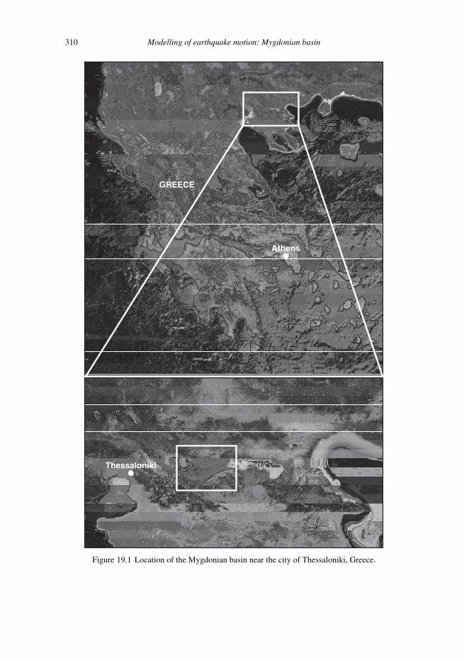
Trim: 247mm × 174mm Top: 14.762mm Gutter: 23.198mmCUUK2497-19 CUUK2497/Moczo ISBN: 978 1 107 02881 4 November 18, 2013 20:42
310 Modelling of earthquake motion: Mygdonian basin
GREECE
Athens
Thessaloniki
Figure 19.1 Location of the Mygdonian basin near the city of Thessaloniki, Greece.

Trim: 247mm × 174mm Top: 14.762mm Gutter: 23.198mmCUUK2497-19 CUUK2497/Moczo ISBN: 978 1 107 02881 4 November 18, 2013 20:42
19.2 Mygdonian basin near Thessaloniki, Greece 311
Table 19.1 Material parameters of two variants of the Mygdonian basin model in E2VP
3D model with homogeneouslayers
3D model withconstant-gradient layers
VS VP ρ VS VP ρ
Layer (m/s) (m/s) (kg/m3) QS (m/s) (m/s) (kg/m3) QS QP
1 200 1500 2100 20 200–250 1500–1600 2100 20–25 ∞2 350 1800 2200 35 250–500 1600–2200 2100–2130 25–50 ∞3 650 2500 2200 65 500–900 2200–2800 2130–2250 50–90 ∞Bedrock 2600 4500 2600 260 2600 4500 2600 260 ∞
690000 695000 700000
4500000
4505000
45100000
690000 695000 700000 690000 695000 700000
Layer 1 Layer 2 Layer 3
70 m 0 160 m 0 420 m
TST TST TST
Figure 19.2 Geometry of a 3D model of the Mygdonian basin. Left: interface between the uppermostand middle sedimentary layers; middle: interface between the middle and bottom sedimentary layers;right: interface the between bottom sedimentary layer and bedrock. TST is the abbreviation for thelocation of a local seismic station.
The model with homogeneous sediment layers can be characterized by
� complicated geometry of the internal interfaces in sediments and the sediment–bedrockinterface,
� relatively low VS in layer 1,� large VS contrast between sediments and bedrock ranging from 4 to 13,� large VP /VS in layer 1 (7.5) and layer 2 (>5).
These characteristics indicate that the numerical modelling of seismic motion is far fromtrivial, especially as modelling was considered for frequencies up to 4 Hz. The modelwith constant-gradient layers is free of (zero-order) discontinuities of material parametersthemselves inside the sediments – only the first spatial derivatives of the material parametersare discontinuous at the interfaces between layers. The absence of zero-order discontinuitiesmakes the gradient model easier for numerical modelling of wave propagation. Becauseexact solutions for the two variant models do not exist, it is reasonable to verify thecapability of a numerical-modelling method using simplified (canonical) models – prior

Trim: 247mm × 174mm Top: 14.762mm Gutter: 23.198mmCUUK2497-19 CUUK2497/Moczo ISBN: 978 1 107 02881 4 November 18, 2013 20:42
312 Modelling of earthquake motion: Mygdonian basin
Table 19.2 Parameters of the elastic models Can2 and Can3. H denotes thickness.
Can2 Can3
H VS VP ρ VS VP ρ
(m) (m/s) (m/s) (kg/m3) (m/s) (m/s) (kg/m3)
17.3 200 1500 2100 200–250 1500–1600 210072.5 350 1800 2200 250–500 1600–2200 2100–2130
115.6 650 2500 2200 500–900 2200–2800 2130–2250inf. 2600 4500 2600 2600 4500 2600
0 1000 2000 3000300
250
200
150
100
50
0
dept
h[m
]
S-wave speed [m/s]0 1000 2000 3000
300
250
200
150
100
50
0
dept
h[m
]
S-wave speed [m/s]
Can2 Can3
Figure 19.3 S-wave speed as a function of depth. Left: model Can2; right: model Can3.
to the numerical simulation for the available realistic complex models. The canonicalmodels should enable testing of the method for crucial aspects associated with the realisticmodels.
19.2.3 Comparative modelling for stringent canonical models
Six canonical models, Can0 – Can5, were designed for testing in E2VP, which can also beused for testing new numerical schemes in difficult conditions. Complete descriptions areavailable at www.sismowine.org. Here we focus on Can2 – Can4.
Can2 – 1D structure consisting of three horizontal homogeneous elastic isotropic layersover a halfspace, 3D wavefield generated by a single vertical force at the free surfaceand a point double-couple source at 3 km depth in the halfspace. The model repre-sents the vertical profile beneath the TST seismic station in the Mygdonian basin.Table 19.2 shows the parameters of the model, the VS profile is illustrated inFig. 19.3(left). The numerical simulations are performed for frequencies up to 4Hz.

Trim: 247mm × 174mm Top: 14.762mm Gutter: 23.198mmCUUK2497-19 CUUK2497/Moczo ISBN: 978 1 107 02881 4 November 18, 2013 20:42
19.2 Mygdonian basin near Thessaloniki, Greece 313
The right-handed Cartesian coordinate system is considered with x positive north, y positiveeast, z positive downward. The single vertical force �f = (0, 0, s) (positive downward) atthe free surface is at the origin of the coordinate system (0, 0, 0). The force time historyis s(t) = 5 · 1011 D(t) where D(t) is a band-pass filtered Dirac delta function. The pointdouble-couple (DC) acts at (0, 0, 3000) m, strike is 22.5°, dip 90°, rake 0°, scalar seismicmoment 1018 N m, and the moment time history is the time integral of D(t).
Figure 19.4 shows the vertical component of the particle velocity at a receiver (2828.4,2828.4, 0) m at the free surface at the xy grid diagonal at a distance of 4000 m. Note thatthe wavelengths at 1 and 4 Hz in the uppermost layer with VS = 200 m/s are 200 and 50 m,respectively. Given the vertical point force at the surface, strong surface Rayleigh waves(consisting mainly of the fundamental and first higher modes) are developed along the xygrid diagonal. In the four panels we show four different FD solutions obtained by the (2,4)velocity–stress staggered-grid scheme using grid spacing h = 5 m. The solutions differfrom each other by the effective grid elastic moduli and density (see Section 9.1), that is,by discrete material representation:
LOC – local (point) values of the elastic moduli and density,ARI – volume arithmetic averages of the elastic moduli and volume arithmetic averages
of the density evaluated using numerical integration over a grid cell centred at thegrid position of the elastic modulus or density,
HAR – volume harmonic averages of the elastic moduli and volume arithmetic averagesof density evaluated using numerical integration over a grid cell centred at the gridposition of the elastic modulus or density; see Subsection 9.2.5,
ORT – volume effective coefficients corresponding to the orthorhombic averagedmedium; see Subsection 9.2.3.
The LOC, ARI and HAR types of material representation are isotropic whereas the ORTtype is anisotropic. Note a very important aspect of the FD modelling: the material interfacesdo not coincide with a grid plane in the two applied grids. In other words, the materialinterfaces go through the interior of the grid cells. The geometry of the interfaces isaccounted for solely by evaluating effective grid material parameters.
The FD seismogram in each panel is shown together with the reference solution obtainedby Emmanuel Chaljub using the DWN codes – Axitra (Bouchon 1981, Coutant 1989) forthe deep DC source and a code developed by Yoshiaki Hisada (Hisada 1994, 1995) for thesurface force. The level of agreement between the FD and DWN seismograms in phaseand amplitude is quantified using the time–frequency phase and envelope goodness-of-fit(GOF) criteria, respectively; see Appendix. We use here the positive-valued goodness-of-fitinstead of the time–frequency misfit criteria due to restriction to the greyscale figure.
As expected (based on our numerical experience), the LOC material representationyields the worst result – the smallest GOF values, especially for Rayleigh waves. TheARI representation yields a very good result. This is because the material interfaces arehorizontal and the dominant wave group, the Rayleigh waves, propagates in the horizontaldirection. A more detailed examination of the body-wave group (in the time window

Trim: 247mm × 174mm Top: 14.762mm Gutter: 23.198mmCUUK2497-19 CUUK2497/Moczo ISBN: 978 1 107 02881 4 November 18, 2013 20:42
314 Modelling of earthquake motion: Mygdonian basin
ORT
4 8 12 16 20 24 28 32 s
1
2
34
1
2
34
4 8 12 16 20 24 28 32
freq
uenc
y[H
z]fr
eque
ncy
[Hz]
-10
10 HAR
s
ARI
4 8 12 16 20 24 28 32 s
1
2
34
1
2
34
freq
uenc
y[H
z]fr
eque
ncy
[Hz]
-10
10 LOC
4 8 12 16 20 24 28 32 s
envelope GOF
phase GOF
vertical component of the particle velocity
envelope GOF
phase GOF
vertical component of the particle velocity
FD solution DWN solution0 5 10
Figure 19.4 FD (grey) and DWN (black) seismograms for Can2. The FD seismograms are obtainedfor h = 5 m using four different material representations – LOC, ARI, HAR and ORT. The levelof agreement between the FD and DWN seismograms in phase and amplitude is quantified usingthe time–frequency phase and envelope goodness-of-fit criteria, respectively. Phase and envelopeGOF = 10 mean that the compared seismograms are the same.
of 1–9 s) using the locally normalized time–frequency misfit would show that ARI is worsethan HAR and ORT. This is because the body-wave group is generated by the deep DCsource in the halfspace. Note that the ARI representation yields considerably worse results(compared to HAR and ORT) as soon as waves do not propagate along an interface. Let
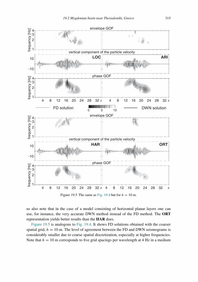
Trim: 247mm × 174mm Top: 14.762mm Gutter: 23.198mmCUUK2497-19 CUUK2497/Moczo ISBN: 978 1 107 02881 4 November 18, 2013 20:42
19.2 Mygdonian basin near Thessaloniki, Greece 315
ORT
4 8 12 16 20 24 28 32 s
1
2
34
1
2
34
4 8 12 16 20 24 28 32
freq
uenc
y[H
z]fr
eque
ncy
[Hz]
-10
10 HAR
s
ARI
4 8 12 16 20 24 28 32 s
1
2
34
1
2
34
freq
uenc
y[H
z]fr
eque
ncy
[Hz]
-10
10 LOC
4 8 12 16 20 24 28 32 s
envelope GOF
phase GOF
vertical component of the particle velocity
envelope GOF
phase GOF
vertical component of the particle velocity
FD solution DWN solution0 5 10
Figure 19.5 The same as Fig. 19.4 but for h = 10 m.
us also note that in the case of a model consisting of horizontal planar layers one canuse, for instance, the very accurate DWN method instead of the FD method. The ORTrepresentation yields better results than the HAR does.
Figure 19.5 is analogous to Fig. 19.4. It shows FD solutions obtained with the coarserspatial grid, h = 10 m. The level of agreement between the FD and DWN seismograms isconsiderably smaller due to coarse spatial discretization, especially at higher frequencies.Note that h = 10 m corresponds to five grid spacings per wavelength at 4 Hz in a medium
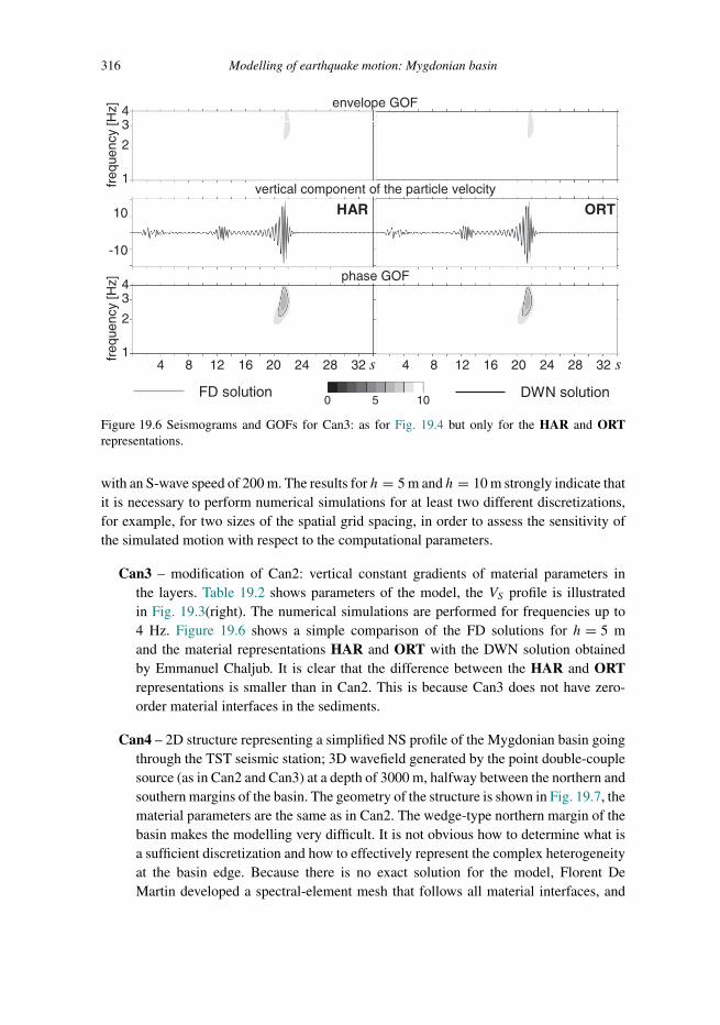
Trim: 247mm × 174mm Top: 14.762mm Gutter: 23.198mmCUUK2497-19 CUUK2497/Moczo ISBN: 978 1 107 02881 4 November 18, 2013 20:42
316 Modelling of earthquake motion: Mygdonian basin
4 8 12 16 20 24 28 32 s
1
2
34
1
2
34
freq
uenc
y[H
z]fr
eque
ncy
[Hz]
-10
10
4 8 12 16 20 24 28 32 s
envelope GOF
phase GOF
vertical component of the particle velocity
FD solution DWN solution0 5 10
ORTHAR
Figure 19.6 Seismograms and GOFs for Can3: as for Fig. 19.4 but only for the HAR and ORTrepresentations.
with an S-wave speed of 200 m. The results for h = 5 m and h = 10 m strongly indicate thatit is necessary to perform numerical simulations for at least two different discretizations,for example, for two sizes of the spatial grid spacing, in order to assess the sensitivity ofthe simulated motion with respect to the computational parameters.
Can3 – modification of Can2: vertical constant gradients of material parameters inthe layers. Table 19.2 shows parameters of the model, the VS profile is illustratedin Fig. 19.3(right). The numerical simulations are performed for frequencies up to4 Hz. Figure 19.6 shows a simple comparison of the FD solutions for h = 5 mand the material representations HAR and ORT with the DWN solution obtainedby Emmanuel Chaljub. It is clear that the difference between the HAR and ORTrepresentations is smaller than in Can2. This is because Can3 does not have zero-order material interfaces in the sediments.
Can4 – 2D structure representing a simplified NS profile of the Mygdonian basin goingthrough the TST seismic station; 3D wavefield generated by the point double-couplesource (as in Can2 and Can3) at a depth of 3000 m, halfway between the northern andsouthern margins of the basin. The geometry of the structure is shown in Fig. 19.7, thematerial parameters are the same as in Can2. The wedge-type northern margin of thebasin makes the modelling very difficult. It is not obvious how to determine what isa sufficient discretization and how to effectively represent the complex heterogeneityat the basin edge. Because there is no exact solution for the model, Florent DeMartin developed a spectral-element mesh that follows all material interfaces, and

Trim: 247mm × 174mm Top: 14.762mm Gutter: 23.198mmCUUK2497-19 CUUK2497/Moczo ISBN: 978 1 107 02881 4 November 18, 2013 20:42
19.2 Mygdonian basin near Thessaloniki, Greece 317
17.3 m72.5 m
115.6 m
1.5 km 3.5 km
simplified geometryof the basin edge
South
the layering is the same as in the Can2 and Can3 models[ ]
2.51,
1.5
2.5, 2.5
xz H Min
x
−= ⋅
∈ −
North
Figure 19.7 Geometry of the 2D structure in the Can4 problem.
the minimum size of the element at the northern edge is only 0.5 m. Such a finediscretization is necessary for SEM in order to reach sufficient accuracy in thewedge-type northern margin. This is because one has to ‘follow’ the discontinuitiesin an SEM in order to get sufficient accuracy. The spectral-element (SE) simulationperformed by the code written by De Martin took 40 days on a 128 core cluster.Though only relative and indicative, in practice the numbers mean that the obtainedsolution can be considered a sufficiently accurate reference for our FD solutions thatuse a uniform grid in which the material interfaces go through the interiors of the gridcells. Recall that the geometry of the interfaces is accounted for solely by evaluatingeffective grid material parameters. Figure 19.8 compares our FD solutions at onereceiver close to the northern edge and one receiver close to the southern edge of thebasin (both receivers and the point source are in one vertical plane) with the referenceSE solution obtained by Florent De Martin. Three FD solutions are obtained withh = 5 m, using the ARI, HAR and ORT representations.
The conclusions for the three representations are:
– The ORT representation yields FD seismograms that are in excellent agreement withthe SE reference solutions at both receivers.
– The HAR representation yields FD seismograms that are in excellent agreement withthe SE reference solution at receiver R1. The motion at R2 is dominated by surfacewaves generated at both the northern and southern edges and propagating along thehorizontal interfaces. The latter fact likely causes the difference between the FD and SEseismograms at receiver R2 after 16 s.
– The ARI representation yields results worse than those obtained with the HAR and ORTrepresentations at receiver R1. At receiver R2 the ARI representation yields results noworse than those obtained with the HAR representation.

Trim: 247mm × 174mm Top: 14.762mm Gutter: 23.198mmCUUK2497-19 CUUK2497/Moczo ISBN: 978 1 107 02881 4 November 18, 2013 20:42
318 Modelling of earthquake motion: Mygdonian basin
ORT
1
2
34
1
2
34
freq
uenc
y[H
z]fr
eque
ncy
[Hz]
-50
50 HAR
envelope GOF
phase GOF
y- component of the particle velocity
FD solution SE solution0 5 10
ARI
envelope GOF
phase GOF
y- component of the particle velocity
SouthNorthR1
(a)
4 8 12 16 20 s
4 8 12 16 20 s4 8 12 16 20 s
Figure 19.8 (a) FD (grey) and SE (black) seismograms for Can4. The FD seismograms are obtainedfor h = 5 m using three different material representations – ARI, HAR and ORT. (b), (c) and (d)differ from (a) by the receiver or the component of the particle velocity – as indicated directly in thefigure.
Each of the three FD simulations took approximately 28 hours on 256 cores. This is anexample of the computational efficiency of FD modelling with proper material parameter-ization.
The main conclusion is: The ORT representation gives excellent results for both R1 andR2 configurations. The HAR representation gives comparable results if the wavefield is not

Trim: 247mm × 174mm Top: 14.762mm Gutter: 23.198mmCUUK2497-19 CUUK2497/Moczo ISBN: 978 1 107 02881 4 November 18, 2013 20:42
19.2 Mygdonian basin near Thessaloniki, Greece 319
ORT
1
2
34
1
2
34
freq
uenc
y[H
z]fr
eque
ncy
[Hz]
-20
20 HAR
ARI
envelope GOF
phase GOF
vertical component of the particle velocity
envelope GOF
phase GOF
vertical component of the particle velocity
FD solution SE solution0 5 10
SouthNorthR1
(b)
4 8 12 16 20 s
4 8 12 16 20 s4 8 12 16 20 s
Figure 19.8 (continued)
dominated by surface waves propagating along horizontal material interfaces. There is noreason to use the ARI representation.
Complete comparison of simulations by the (2,4) velocity–stress staggered-grid scheme(Kristek and Moczo), (4,4) velocity–stress collocated-grid scheme (Z. Zhang, W. Zhangand Chen), spectral-element method (Chaljub and De Martin), and Fourier pseudo-spectralmethod (Klin and Priolo) is the subject of a journal article.

Trim: 247mm × 174mm Top: 14.762mm Gutter: 23.198mmCUUK2497-19 CUUK2497/Moczo ISBN: 978 1 107 02881 4 November 18, 2013 20:42
320 Modelling of earthquake motion: Mygdonian basin
ORT
1
2
34
1
2
34
freq
uenc
y[H
z]fr
eque
ncy
[Hz]
-50
50 HAR
envelope GOF
phase GOF
y- component of the particle velocity
FD solution SE solution0 5 10
ARI
envelope GOF
phase GOF
y- component of the particle velocity
SouthNorthR2
(c)
4 8 12 16 20 s
4 8 12 16 20 s4 8 12 16 20 s
Figure 19.8 (continued)
19.2.4 Modelling for the realistic three-layered viscoelastic model
Here we illustratively compare the FD ORT simulation ( h = 5 m) with the SE simula-tion obtained by Emmanuel Chaljub using the SPECFEM3D code developed by DimitriKomatitsch and Jeroen Tromp (e.g., Komatitsch and Tromp 1999, Tromp et al. 2008, Peteret al. 2011).
The model was described in Subsection 19.2.2. The wavefield is generated by a double-couple source beneath TST at a depth of 3 km.
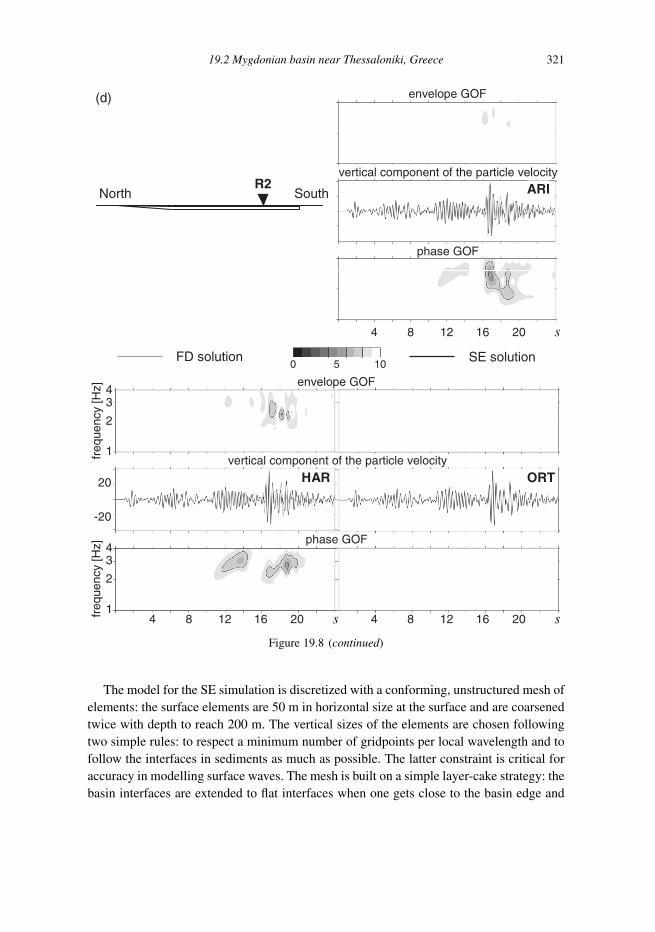
Trim: 247mm × 174mm Top: 14.762mm Gutter: 23.198mmCUUK2497-19 CUUK2497/Moczo ISBN: 978 1 107 02881 4 November 18, 2013 20:42
19.2 Mygdonian basin near Thessaloniki, Greece 321
ORT
1
2
34
1
2
34
freq
uenc
y[H
z]fr
eque
ncy
[Hz]
-20
20 HAR
envelope GOF
phase GOF
vertical component of the particle velocity
FD solution SE solution0 5 10
ARI
4 8 12 16 20 s
envelope GOF
phase GOF
vertical component of the particle velocity
SouthNorthR2
(d)
4 8 12 16 20 s4 8 12 16 20 s
Figure 19.8 (continued)
The model for the SE simulation is discretized with a conforming, unstructured mesh ofelements: the surface elements are 50 m in horizontal size at the surface and are coarsenedtwice with depth to reach 200 m. The vertical sizes of the elements are chosen followingtwo simple rules: to respect a minimum number of gridpoints per local wavelength and tofollow the interfaces in sediments as much as possible. The latter constraint is critical foraccuracy in modelling surface waves. The mesh is built on a simple layer-cake strategy: thebasin interfaces are extended to flat interfaces when one gets close to the basin edge and

Trim: 247mm × 174mm Top: 14.762mm Gutter: 23.198mmCUUK2497-19 CUUK2497/Moczo ISBN: 978 1 107 02881 4 November 18, 2013 20:42
322 Modelling of earthquake motion: Mygdonian basin
50 10 15 20 25 s 50 10 15 20 25 s
-1
0
1
-1
0
1
-1
0
1
N N
E E
Z Z
FD solution SE solutionP
artic
leve
loci
ty[1
0-6 m
/s]
Figure 19.9 The FD ORT and SE seismograms for the realistic 3D viscoelastic model, TST station.
each modified layer is filled with the same number of elements in the vertical direction. Theresulting numerical representation of the interfaces is not uniform: it is optimized withinthe central part of the basin but not close to the edges. The smallest (vertical) element sizeis found in the first layer of the model and equals 2.5 m.
The SE simulation does not serve as a reference solution at the same level of accuracy asthe SE solution for Can4, and the visual comparison of the FD ORT and SE seismogramsin Fig. 19.9 is illustrative.
Recall that all the numerical solutions presented and mentioned in this chapter togetherwith detailed descriptions of the computational models are available at www.sismowine.org.
Finally, let us note that we do not present simulations for real local earthquakes. Atthe time of preparation of the book, the numerical simulations in E2VP had not reached asatisfactory level of agreement with records. Additional investigations strongly indicatedthe possibility that the available structural model should be improved.
19.2.5 Lessons learned from ESG 2006 and E2VP
The ESG 2006 comparative exercise (Chaljub et al. 2010) and numerous detailed compara-tive analyses performed in E2VP lead to conclusions important for the practical applicationof numerical methods in predicting earthquake ground motion at a site of interest:
Methodological – general� There is no single numerical-modelling method that can be considered the best –
in terms of accuracy and computational efficiency – for all structure–wavefieldconfigurations important for predicting earthquake ground motion in surface localstructures.
� Apparently and intuitively, ‘small’ or ‘insignificant’ differences in the discreterepresentation of spatial variations in material parameters can cause considerable

Trim: 247mm × 174mm Top: 14.762mm Gutter: 23.198mmCUUK2497-19 CUUK2497/Moczo ISBN: 978 1 107 02881 4 November 18, 2013 20:42
19.2 Mygdonian basin near Thessaloniki, Greece 323
inaccuracies and consequently discrepancies in predictions obtained by differentmethods.
� Sufficiently accurate and computationally efficient methods for implementing con-tinuous and discontinuous material heterogeneity (consistent with the interfaceboundary condition), realistic attenuation (no simpler than that corresponding tothe GZB/GMB-EK rheology), a nonreflecting boundary (no less efficient thanPML) and free-surface conditions prove to be the key elements of a reasonablyaccurate numerical simulation.
Methodological – FD method� The commonly used name of ‘finite-difference method’ in numerical modelling of
earthquake ground motion may represent one of a large variety of FD schemes andcodes. Surprisingly, not all FD schemes used for simulations and publications areat the state-of-the-art level: the available methods and techniques for representingspatial material heterogeneity, realistic attenuation, large VP /VS , free surfacesand nonreflecting boundaries of the grid are not implemented in some frequentlyapplied codes.
Practical� The numerical-simulation methods and the corresponding computer codes are not
yet in a ‘press-button’ mode; the codes should never be applied as black-box tools,that is, without sufficient methodological knowledge of the method and the code.
� At least two different but comparably accurate, verified and state-of-the-art meth-ods should be applied in order to obtain reliable numerical prediction of earthquakeground motion at a site of interest.
� Material interfaces should not be artificially introduced in the computational model;their presence can have a strong impact on the locally induced surface waves.
� It is necessary to perform numerical simulations for at least two different dis-cretizations, e.g., for two sizes of the spatial grid spacing or element, in order toassess the sensitivity of the simulated motion with respect to the computationalparameters.

Trim: 247mm × 174mm Top: 14.762mm Gutter: 23.198mmCUUK2497-CON CUUK2497/Moczo ISBN: 978 1 107 02881 4 November 18, 2013 19:56
Concluding remarks: search for the best scheme
We have mentioned several times that no single numerical-modelling method developedso far is better than other methods for all important configurations of the medium andwavefield. Being better for a particular problem configuration means:
– either being more accurate at some level of computational efficiency (quantified in termsof requirements on computer time and memory)
– or being more computational efficient at an optional level of accuracy.
A method or scheme applicable to a wider class of medium–wavefield configurationsis not necessarily the most efficient method for some important configurations to whichother (possibly less universal) methods are applicable. In fact, the less universal methodmight be considerably more efficient for some configurations at the same level of accu-racy. The importance of computational efficiency increases with complexity of the modeland maximum frequency up to which the numerical modelling should be sufficientlyaccurate.
In view of what we have just said about the numerical methods in general, can oneparticular FD scheme be better than other schemes for all important problem configurations?It is not easy to answer in a rigorous and comprehensive manner – especially at the presentstate of development and elaboration of the FD schemes, which certainly is far from whatis in principle possible. It is, however, very likely that what we said about all numerical-modelling methods is also true about all possible FD schemes.
We may, however, think of properties of a hypothetical best FD scheme for a certainclass of important problems. The best scheme should be consistent with the mathematical-physical problem with an optional level of accuracy (e.g., with an optional and the sameorder of accuracy in space and time), stable, and computationally efficient.
Particular properties of the best FD scheme for modelling earthquake motions shouldinclude:
– stability at a� free surface (planar and nonplanar),� contact of the free surface with internal material interface,� contact of the free surface with the PML,
324

Trim: 247mm × 174mm Top: 14.762mm Gutter: 23.198mmCUUK2497-CON CUUK2497/Moczo ISBN: 978 1 107 02881 4 November 18, 2013 19:56
Concluding remarks: search for the best scheme 325
� contact of the internal material interface and the PML and, if a water layer is animportant part of the structural model, also
� liquid–solid interface,– optional level of accuracy
� for any value of the P-wave to S-wave speed ratio, that is VP /VS ∈ [√
2,∞], or,equivalently, for any value of Poisson’s ratio, that is σ ∈ [0, 0.5],
� in a medium with strong gradient of material parameters,� in a medium with strong contrast of material parameters at an internal interface,� in a medium with material interfaces not coinciding with grid planes or grid lines,� at and near the free surface (planar and nonplanar),� in an attenuative medium,� at and near a rupturing fault (planar and nonplanar),� of implementation of a kinematic source,
– computational efficiency in terms of� relatively low memory,� relatively short computational time.
Can all particle-velocity and stress-tensor components at each grid position of a curvilin-ear grid, relatively small stencils for approximating derivatives, and a proper effective gridrepresentation of material properties or some other ingredients make it possible to achievebetter schemes? Recent intensive effort to develop new, more accurate and more efficientschemes indicates several strategies. The future will show which of them will make it pos-sible to apply the FD method further and better than before in earthquake ground motionmodelling and prediction.

Trim: 247mm × 174mm Top: 14.762mm Gutter: 23.198mmCUUK2497-CON CUUK2497/Moczo ISBN: 978 1 107 02881 4 November 18, 2013 19:56

Trim: 247mm × 174mm Top: 14.762mm Gutter: 23.198mmCUUK2497-APP CUUK2497/Moczo ISBN: 978 1 107 02881 4 November 19, 2013 17:32
Appendix A
Time–frequency misfit and goodness-of-fit criteriafor quantitative comparison of time signals
In the process of development and verification of a numerical method for calculation ofseismic wave propagation it is necessary to quantitatively compare a numerically simulatedsignal with a reference or exact solution. In the process of validation of the numericalmethod it is necessary to quantitatively compare a numerically simulated signal with aseismic record. Comparison of two recorded signals significantly helps in the analysis andinterpretation of the process under investigation. The quantitative misfit and goodness-of-fitcriteria introduced by Kristekova et al. (2006, 2009) are summarized and explained in thisappendix.
A.1 Characterization of a signal
Here we restrict our discussion to basic concepts and relations for characterising a signalnecessary in the further exposition.
A.1.1 Simplest characteristics
Consider the simplest case of a monochromatic signal:
sm(t) = A cos(2πf t + φ) (A.1)
where t is time, A is amplitude, φ is phase and f is frequency. Signal characteristics A, φand f are unambiguously defined and very easy to interpret. If a signal is more complicated,the notion of amplitude, phase and frequency may be not so obvious. For example, whenA = A(t), and f = f (t) and φ = φ(t) in the argument of the cosine function, the amplitudeand phase are ambiguous.
The analytical signal (e.g., Flandrin 1999) enables us to develop proper unambiguouscharacteristics. The analytical signal s(t) with respect to signal s(t) is
s(t) = s(t) + iH {s(t)} (A.2)
where H {s(t)} is the Hilbert transform of signal s(t). Relations
A(t) = |s(t)|, φ(t) = Arg[s(t)] (A.3)
and
f (t) = 1
2π
dArg[s(t)]
dt(A.4)
327

Trim: 247mm × 174mm Top: 14.762mm Gutter: 23.198mmCUUK2497-APP CUUK2497/Moczo ISBN: 978 1 107 02881 4 November 19, 2013 17:32
328 Appendix A: Time–frequency misfit and goodness-of-fit criteria
define the envelope, phase and (so-called instantaneous) frequency of the signal at time t .Although these quantities are unambiguous, in fact they represent just averaged values. Forexample, Qian (2002) suggests using the term ‘mean instantaneous frequency’ instead ofthe instantaneous frequency. The narrower is the spectral content at time t , the better is theestimate of the dominant amplitude, phase and frequency by Eqs. (A.3) and (A.4).
Clearly, the analytical signal cannot be used for determining the three basic characteris-tics of a signal if its spectral content is complicated and changes with time.
A.1.2 Time–frequency decomposition
The instantaneous spectral content or time evolution at any frequency of a signal, andhence the time evolution of the spectral content of the signal, can be obtained using thetime–frequency (TF) representation of the signal. The TF representation can be calculatedusing, for example, the continuous wavelet transform (CWT). The CWT of signal s(t) isdefined by
CWT(a,b){s(t)} = 1√|a|∫ ∞
−∞s(t)ψ∗
(t − ba
)dt (A.5)
with a being the scale parameter, b the translational parameter, andψ the analyzing wavelet.The asterisk denotes the complex conjugate function. The scale parameter a is inverselyproportional to frequency f . Consider an analyzing wavelet with a spectrum that has zeroamplitudes at negative frequencies. Such a wavelet is an analytical signal and is called theprogressive wavelet. A Morlet wavelet
ψ(t) = π−1/4 exp(iω0t) exp(−t2/2) (A.6)
with ω0 = 6s−1, is a proper choice for a wide class of signals and problems, and can beconsidered as a progressive wavelet. The TF representation of signal s(t) based on theCWT, W (t, f ), can be then defined by choosing a relation between the scale parameter aand frequency f . Assume
a = ω0/2πf (A.7)
Then,
W (t, f ) = CWT(a,b){s(t)} =√
2π |f |ω0
∫ ∞
−∞s(τ )ψ∗
(2πf
τ − tω0
)dτ (A.8)
W 2(t, f ) represents the energy distribution (energy density) of the signal in the TF plane.See, for example, the monographs by Daubechies (1992) and Holschneider (1995) forcomprehensive expositions of the CWT and Morlet wavelet. The useful properties of theCWT for the TF analysis of complicated seismic records have been demonstrated byKristekova et al. (2008) and others. Their analysis of seismic records led to identificationof a sequence of relatively weak explosions.
Having determined the TF representation, an envelope A(t, f ) and phase φ(t, f ) at agiven point of the TF plane can be defined:
A(t, f ) = |W (t, f )|, φ(t, f ) = Arg[W (t, f )] (A.9)

Trim: 247mm × 174mm Top: 14.762mm Gutter: 23.198mmCUUK2497-APP CUUK2497/Moczo ISBN: 978 1 107 02881 4 November 19, 2013 17:32
A.2 Comparison of signals 329
Holschneider (1995) showed that ifW (t, f ) is defined using the CWT with the progressivewavelet, envelope A(t, f ) and phase φ(t, f ) are consistent with those defined using theanalytical signal.
Note that the TF representation obtained using the CWT is more suitable for the analysisof complicated nonstationary signals than the TF representation obtained using the win-dowed Fourier transform. This is because the CWT is not limited by the fixed TF resolutionas it is in the case of the windowed Fourier transform.
A.2 Comparison of signals
A.2.1 TF envelope and phase differences
Consider a signal s(t) and a reference signal sref(t). Given Eqs. (A.8) and (A.9) it is clearthat
�A(t, f ) = A(t, f ) − Ar(t, f ) = |W (t, f )| − |Wr(t, f )| (A.10)
defines the difference between the envelopes of signals s(t) and sref(t) at each (t, f ) point.Similarly,
�φ(t, f ) = φ(t, f ) − φr(t, f ) = Arg[W (t, f )] − Arg[Wr(t, f )] (A.11)
defines the difference between two phases at each (t, f ) point.The envelope difference �A(t, f ) is a local difference that can attain any value. The
local phase difference needs some explanation. A little complication comes from the factthat Arg[ξ ] always gives the phase of the complex variable ξ in the range of (−π, π ]. If, say,two phases are 170π/180 and −160π/180, Eq. (A.11) formally gives 330π/180 insteadof the correct value −30π/180. It is clear that definition (A.11) would need an additionalcondition to treat similar situations. Instead, however, we can avoid the additional conditionby using the following equivalent definition:
�φ(t, f ) = Arg
[W (t, f )
Wr(t, f )
](A.12)
Relation (A.12) always gives the local phase difference in the range of (−π, π ].
A.2.2 Locally normalized and globally normalized criteria
Having the local envelope and phase differences at the (t, f ) point, we can define a varietyof TF misfit criteria to quantitatively compare the entire signals, their important parts orcharacteristics of the signals.
Locally normalized criteria In some problems it is important to investigate relativelysmall parts of the signal – no matter how large the amplitudes of those parts are withrespect to the maximum amplitude of the entire signal. In other cases one may be interestedin a detailed TF anatomy of the disagreement between two entire signals including small-amplitude parts. For comparing two signals in such situations we need to define local misfitcriteria – criteria whose values for one (t, f ) point would depend only on the characteristicsat that (t, f ) point.
Consider how to define a local TF misfit criterion for the envelope. It is clear that such acriterion should quantify the relative difference between two envelopes at the (t, f ) point.
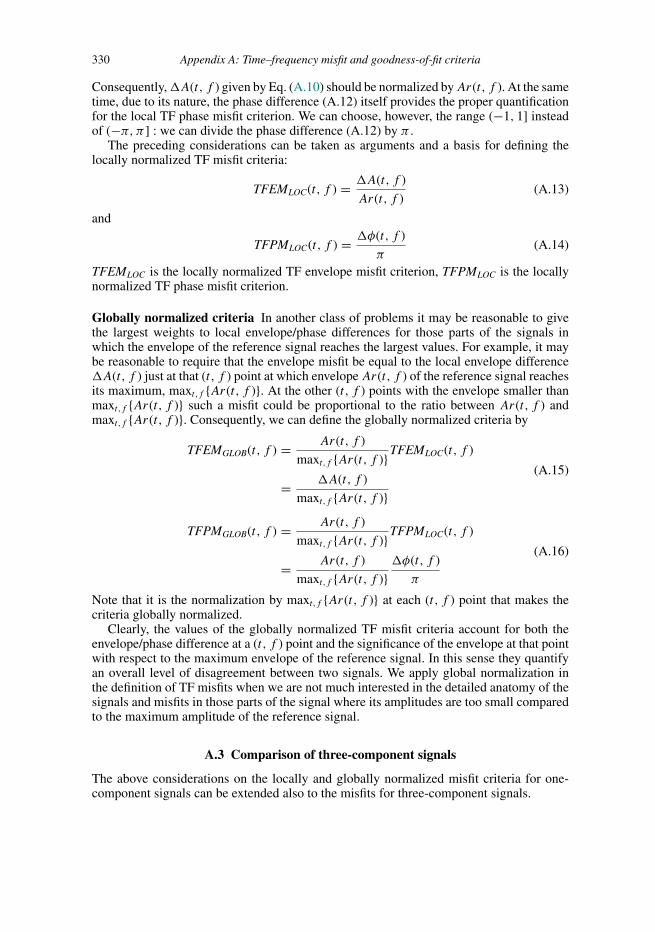
Trim: 247mm × 174mm Top: 14.762mm Gutter: 23.198mmCUUK2497-APP CUUK2497/Moczo ISBN: 978 1 107 02881 4 November 19, 2013 17:32
330 Appendix A: Time–frequency misfit and goodness-of-fit criteria
Consequently,�A(t, f ) given by Eq. (A.10) should be normalized byAr(t, f ). At the sametime, due to its nature, the phase difference (A.12) itself provides the proper quantificationfor the local TF phase misfit criterion. We can choose, however, the range (−1, 1] insteadof (−π, π ] : we can divide the phase difference (A.12) by π .
The preceding considerations can be taken as arguments and a basis for defining thelocally normalized TF misfit criteria:
TFEMLOC(t, f ) = �A(t, f )
Ar(t, f )(A.13)
and
TFPMLOC(t, f ) = �φ(t, f )
π(A.14)
TFEMLOC is the locally normalized TF envelope misfit criterion, TFPMLOC is the locallynormalized TF phase misfit criterion.
Globally normalized criteria In another class of problems it may be reasonable to givethe largest weights to local envelope/phase differences for those parts of the signals inwhich the envelope of the reference signal reaches the largest values. For example, it maybe reasonable to require that the envelope misfit be equal to the local envelope difference�A(t, f ) just at that (t, f ) point at which envelopeAr(t, f ) of the reference signal reachesits maximum, maxt,f {Ar(t, f )}. At the other (t, f ) points with the envelope smaller thanmaxt,f {Ar(t, f )} such a misfit could be proportional to the ratio between Ar(t, f ) andmaxt,f {Ar(t, f )}. Consequently, we can define the globally normalized criteria by
TFEMGLOB(t, f ) = Ar(t, f )
maxt,f {Ar(t, f )}TFEMLOC(t, f )
= �A(t, f )
maxt,f {Ar(t, f )}(A.15)
TFPMGLOB(t, f ) = Ar(t, f )
maxt,f {Ar(t, f )}TFPMLOC(t, f )
= Ar(t, f )
maxt,f {Ar(t, f )}�φ(t, f )
π
(A.16)
Note that it is the normalization by maxt,f {Ar(t, f )} at each (t, f ) point that makes thecriteria globally normalized.
Clearly, the values of the globally normalized TF misfit criteria account for both theenvelope/phase difference at a (t, f ) point and the significance of the envelope at that pointwith respect to the maximum envelope of the reference signal. In this sense they quantifyan overall level of disagreement between two signals. We apply global normalization inthe definition of TF misfits when we are not much interested in the detailed anatomy of thesignals and misfits in those parts of the signal where its amplitudes are too small comparedto the maximum amplitude of the reference signal.
A.3 Comparison of three-component signals
The above considerations on the locally and globally normalized misfit criteria for one-component signals can be extended also to the misfits for three-component signals.
Trim: 247mm × 174mm Top: 14.762mm Gutter: 23.198mmCUUK2497-APP CUUK2497/Moczo ISBN: 978 1 107 02881 4 November 19, 2013 17:32
A.3 Comparison of three-component signals 331
A.3.1 TF misfit criteria
The case: one signal being a reference If the amplitudes of one component of the ref-erence signal are significantly smaller than the amplitudes of two other components (e.g.,a common situation with polarized particle motion), the only reasonable choice for globalnormalization is to take the maximum TF envelope value from all three components ofthe reference signal. This choice naturally quantifies the misfits with respect to meaningfulvalues of the three-component reference signal. It also prevents obtaining too large misfitsdue to possible division by very small envelope values corresponding to insignificant ampli-tudes of the signal components. Clearly, this choice is reasonable also if the amplitudes ofall three components are comparable.
A formal definition of one local normalization factor for all three components wouldclearly contradict the local character of a misfit criterion. Therefore, each component hasto be treated as a ‘one-component’ signal if one is interested in the detailed anatomy of theTF misfit.
Now we can define a set of misfit criteria for the three-component signals when one ofthem can be considered a reference. The locally normalized and globally normalized TFenvelope misfits TFEMREF
LOC,i(t, f ) and TFEMREFGLOB,i(t, f ) characterize how the envelopes of
two signals differ at each (t, f ) point. Similarly, TFPMREFLOC,i(t, f ) and TFPMREF
GLOB,i(t, f )characterize how the phases of two signals differ at each (t, f ) point.
Projections of the TF misfits onto the time domain give the time-dependent envelopeand phase misfits TEMREF
LOC,i(t), TEMREFGLOB,i(t), TPMREF
LOC,i(t) and TPMREFGLOB,i(t). Projections
of the TF misfits onto the frequency domain give the frequency-dependent envelope andphase misfits FEMREF
LOC,i(f ), FEMREFGLOB,i(f ), FPMREF
LOC,i(f ) and FPMREFGLOB,i(f ).
Finally, it is often very useful to have single-valued envelope and phase misfits EMREFLOC,i,
EMREFGLOB,i, PMREF
LOC,i and PMREFGLOB,i. All the misfits are summarized in Table A.1. The envelope
and phase misfits can attain any value in the range (−∞,∞) and (−1, 1], respectively.
The case: no signal being a reference The misfit criteria for this case can be defined,in fact, formally in the same way as criteria in the case with a reference signal. The onlyquestion is, which of the two signals should be formally taken as a reference? The reasonableway is to find a maximum envelope for each of the two signals. Then the signal with thesmaller maximum can be chosen as a reference signal. In the case of the globally normalizedcriteria for the three-component signals the maximum is taken from all components. In thecase of the locally normalized criteria the reference signal should be chosen separately foreach component.
Note that the evaluation of the TF misfits themselves does not give us a reason to preferthe smaller of the two maxima. Our choice comes from the possible link to the goodness-of-fit criteria developed by Anderson (2004). We take the smaller maximum consistentlywith the Anderson criteria.
A.3.2 TF goodness-of-fit criteria
The envelope TF misfits quantify and characterize how much two envelopes differ fromeach other. Correspondingly, the envelope misfit can attain any value within the rangeof (−∞,∞), with 0 meaning the agreement. While formally applicable to any level ofdisagreement, clearly, the envelope misfits are most useful for comparing relatively closeenvelopes.

Trim: 247mm × 174mm Top: 14.762mm Gutter: 23.198mmCUUK2497-APP CUUK2497/Moczo ISBN: 978 1 107 02881 4 November 19, 2013 17:32
332 Appendix A: Time–frequency misfit and goodness-of-fit criteria
Table A.1 TF misfit criteria for three-component signals assuming one of them as areference signal
si (t); i = 1, 2, 3 a three-component signalsri (t); i = 1, 2, 3 a three-component reference signalWi = Wi (t, f ) TF representation of signal si (t)Wri = Wri (t, f ) TF representation of the reference signal sri (t)
Time–frequency envelope and phase misfits
locally normalized TF envelope misfit TFEMREFLOC,i (t, f ) = |Wi | − |Wri |
|Wri |locally normalized TF phase misfit TFPMREF
LOC,i (t, f ) = 1
πArg
[Wi
Wr i
]globally normalized TF
{envelopephase
}misfit{
TFEMREFGLOB,i (t, f )
TFPMREFGLOB,i (t, f )
}= |Wri |
maxi; t,f (|Wri |)
{TFEMREF
LOC,i (t, f )
TFPMREFLOC,i (t, f )
}
Time-dependent envelope and phase misfitslocally normalized
{TEMREF
LOC,i (t)
TPMREFLOC,i (t)
}=
∑f
|Wri |{
TFEMREFLOC,i (t, f )
TFPMREFLOC,i (t, f )
}∑f
|Wri |
globally normalized
{TEMREF
GLOB,i (t)
TPMREFGLOB,i (t)
}=
∑f
|Wri |{
TFEMREFLOC,i (t, f )
TFPMREFLOC,i (t, f )
}
maxi; t
(∑f
|Wri |)
Frequency-dependent envelope and phase misfitslocally normalized
{FEMREF
LOC,i (f )
FPMREFLOC,i (f )
}=
∑t
|Wri |{
TFEMREFLOC,i (t, f )
TFPMREFLOC,i (t, f )
}∑t
|Wri |
globally normalized
{FEMREF
GLOB,i (f )
FPMREFGLOB,i (f )
}=
∑t
|Wri |{
TFEMREFLOC,i (t, f )
TFPMREFLOC,i (t, f )
}
maxi; f
(∑t
|Wri |)
Single-valued envelope and phase misfitslocally normalized
{EMREF
LOC,i
PMREFLOC,i
}=
√√√√√√√√∑f
∑t
|Wri |2∣∣∣∣∣{
TFEMREFLOC,i (t, f )
TFPMREFLOC,i (t, f )
}∣∣∣∣∣2
∑f
∑t
|Wri |2
globally normalized
{EMREF
GLOB,i
PMREFGLOB,i
}=
√√√√√√√√√√∑f
∑t
|Wri |2∣∣∣∣∣{
TFEMREFLOC,i (t, f )
TFPMREFLOC,i (t, f )
}∣∣∣∣∣2
maxi
(∑f
∑t
|Wri |2)
However, in practice it is often necessary to compare signals whose envelopes differconsiderably. Comparison of real records with synthetics in some problems can be a goodexample. In such a case it is reasonable to look for the level of agreement rather than detailsof disagreement. The goodness-of-fit criteria provide a suitable tool for this.
The goodness-of-fit criteria approach a zero value with an increasing level of disagree-ment. On the other hand, some finite value is chosen to quantify the agreement.
The TF envelope goodness-of-fit criteria can be introduced on the basis of the TFenvelope misfits:
TFEG(t, f ) = A exp{−|TFEM(t, f )|k}TEG(t) = A exp{−|TEM(t)|k}
FEG(f ) = A exp{−|FEM(f )|k}EG = A exp{−|EM|k}A > 0, k > 0
(A.17)
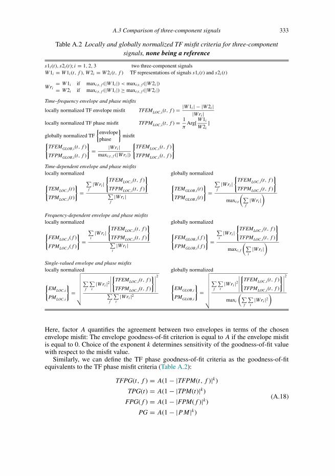
Trim: 247mm × 174mm Top: 14.762mm Gutter: 23.198mmCUUK2497-APP CUUK2497/Moczo ISBN: 978 1 107 02881 4 November 19, 2013 17:32
A.3 Comparison of three-component signals 333
Table A.2 Locally and globally normalized TF misfit criteria for three-componentsignals, none being a reference
s1i (t), s2i (t); i = 1, 2, 3 two three-component signalsW1i = W1i (t, f ),W2i = W2i (t, f ) TF representations of signals s1i (t) and s2i (t)
= W1i if maxi;t,f (|W1i |) < maxi;t,f (|W2i |)Wri = W2i if maxi;t,f (|W1i |) ≥ maxi;t,f (|W2i |)Time–frequency envelope and phase misfits
locally normalized TF envelope misfit TFEMLOC,i(t, f ) = |W1i | − |W2i ||Wri |
locally normalized TF phase misfit TFPMLOC,i(t, f ) = 1
πArg[
W1iW2i
]
globally normalized TF
{envelopephase
}misfit{
TFEMGLOB,i(t, f )
TFPMGLOB,i(t, f )
}= |Wri |
maxi;t,f (|Wri |)
{TFEMLOC,i(t, f )
TFPMLOC,i(t, f )
}
Time-dependent envelope and phase misfitslocally normalized
{TEMLOC,i(t)
TPMLOC,i(t)
}=
∑f
|Wri |{
TFEMLOC,i(t, f )
TFPMLOC,i(t, f )
}∑f
|Wri |
globally normalized
{TEMGLOB,i(t)
TPMGLOB,i(t)
}=
∑f
|Wri |{
TFEMLOC,i(t, f )
TFPMLOC,i(t, f )
}
maxi;t
(∑f
|Wri |)
Frequency-dependent envelope and phase misfitslocally normalized
{FEMLOC,i(f )
FPMLOC,i(f )
}=
∑t
|Wri |{
TFEMLOC,i(t, f )
TFPMLOC,i(t, f )
}∑t
|Wri |
globally normalized
{FEMGLOB,i(f )
FPMGLOB,i(f )
}=
∑t
|Wri |{
TFEMLOC,i(t, f )
TFPMLOC,i(t, f )
}
maxi;f
(∑t
|Wri |)
Single-valued envelope and phase misfitslocally normalized
{EMLOC,i
PMLOC,i
}=
√√√√√√√√∑f
∑t
|Wri |2∣∣∣∣∣{
TFEMLOC,i(t, f )
TFPMLOC,i(t, f )
}∣∣∣∣∣2
∑f
∑t
|Wri |2
globally normalized
{EMGLOB,i
PMGLOB,i
}=
√√√√√√√√√∑f
∑t
|Wri |2∣∣∣∣∣{
TFEMLOC,i(t, f )
TFPMLOC,i(t, f )
}∣∣∣∣∣2
maxi
(∑f
∑t
|Wri |2)
Here, factor A quantifies the agreement between two envelopes in terms of the chosenenvelope misfit: The envelope goodness-of-fit criterion is equal to A if the envelope misfitis equal to 0. Choice of the exponent k determines sensitivity of the goodness-of-fit valuewith respect to the misfit value.
Similarly, we can define the TF phase goodness-of-fit criteria as the goodness-of-fitequivalents to the TF phase misfit criteria (Table A.2):
TFPG(t, f ) = A(1 − |TFPM(t, f )|k)TPG(t) = A(1 − |TPM(t)|k)
FPG(f ) = A(1 − |FPM(f )|k)PG = A(1 − |PM|k)
(A.18)
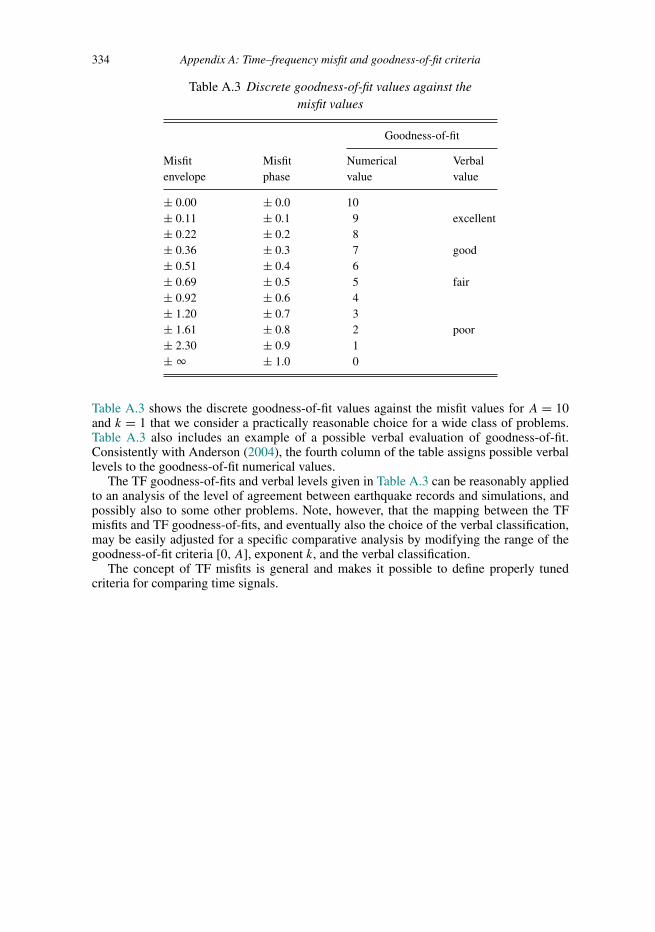
Trim: 247mm × 174mm Top: 14.762mm Gutter: 23.198mmCUUK2497-APP CUUK2497/Moczo ISBN: 978 1 107 02881 4 November 19, 2013 17:32
334 Appendix A: Time–frequency misfit and goodness-of-fit criteria
Table A.3 Discrete goodness-of-fit values against themisfit values
Goodness-of-fit
Misfitenvelope
Misfitphase
Numericalvalue
Verbalvalue
± 0.00 ± 0.0 10± 0.11 ± 0.1 9 excellent± 0.22 ± 0.2 8± 0.36 ± 0.3 7 good± 0.51 ± 0.4 6± 0.69 ± 0.5 5 fair± 0.92 ± 0.6 4± 1.20 ± 0.7 3± 1.61 ± 0.8 2 poor± 2.30 ± 0.9 1± � ± 1.0 0
Table A.3 shows the discrete goodness-of-fit values against the misfit values for A = 10and k = 1 that we consider a practically reasonable choice for a wide class of problems.Table A.3 also includes an example of a possible verbal evaluation of goodness-of-fit.Consistently with Anderson (2004), the fourth column of the table assigns possible verballevels to the goodness-of-fit numerical values.
The TF goodness-of-fits and verbal levels given in Table A.3 can be reasonably appliedto an analysis of the level of agreement between earthquake records and simulations, andpossibly also to some other problems. Note, however, that the mapping between the TFmisfits and TF goodness-of-fits, and eventually also the choice of the verbal classification,may be easily adjusted for a specific comparative analysis by modifying the range of thegoodness-of-fit criteria [0, A], exponent k, and the verbal classification.
The concept of TF misfits is general and makes it possible to define properly tunedcriteria for comparing time signals.

Trim: 247mm × 174mm Top: 14.762mm Gutter: 23.198mmCUUK2497-REF CUUK2497/Moczo ISBN: 978 1 107 02881 4 November 19, 2013 18:0
References
Aagaard, B. T., T. M. Brocher, D. Dolenc, D. S. Dreger, R. W. Graves, S. C. Harmsen, S. H.Hartzell, S. Larsen, M. L. Zoback 2008a. Ground-motion modeling of the 1906 SanFrancisco earthquake, Part I: Validation using the 1989 Loma Prieta Earthquake. Bull.Seism. Soc. Am. 98, 989–1011.
Aagaard, B. T., T. M. Brocher, D. Dolenc, D. S. Dreger, R. W. Graves, S. C. Harmsen,S. H. Hartzell, S. Larsen, K. McCandless, S. Nilsson, N. A. Petersson, A. Rodgers,B. Sjogreen, M. L. Zoback 2008b. Ground-motion modeling of the 1906 San Franciscoearthquake, Part II: Ground-motion estimates for the 1906 earthquake and scenarioevents. Bull. Seism. Soc. Am. 98, 1012–1046.
Aagaard, B. T., T. H. Heaton, J. F. Hall 2001. Dynamic earthquake ruptures in the presenceof lithostatic normal stresses: Implications for friction models and heat production.Bull. Seism. Soc. Am. 91, 1765–1796.
Aboudi, J. 1971. Numerical simulation of seismic sources. Geophysics 36, 810–821.Abreu, R., D. Stich, J. Morales 2013. On the generalization of the complex step method.
J. Comput. Appl. Math. 241, 84–102.Aki, K., P. G. Richards 2002. Quantitative Seismology, 2nd edn. University Science
Books.Alexeev, A. S., B. G. Mikhailenko 1980. The solution of dynamic problems of elastic
wave propagation in inhomogeneous media by a combination of partial separation ofvariables and finite-difference methods. J. Geophys. 48, 161–172.
Alford, R. M., K. R. Kelly, D. M. Boore 1974. Accuracy of finite-difference modeling ofthe acoustic wave equation. Geophysics 39, 834–842.
Alterman, Z. S., F. C. Karal 1968. Propagation of elastic waves in layered media by finitedifference methods. Bull. Seism. Soc. Am. 58, 367–398.
Alterman, Z., D. Loewenthal 1970. Seismic waves in a quarter and three-quarter plane.Geophys. J. R. Astr. Soc. 20, 101–126.
Alterman, Z. S., R. Nathaniel 1975. Seismic waves in a wedge. Bull. Seism. Soc. Am. 65,1697–1719.
Alterman, Z. S., A. Rotenberg 1969. Seismic waves in a quarter plane. Bull. Seism. Soc.Am. 59, 347–368.
Ampuero, J.-P. 2002. Etude physique et numerique de la nucleation des seismes. PhDThesis. Universite Paris 7, Denis Diderot.
Ampuero, J.-P. 2008. SEM2DPACK: A spectral element method for 2D wave propagationand earthquake source dynamics, version 2.3.3, available at http://sourceforge.net/projects/sem2d/.
335
Trim: 247mm × 174mm Top: 14.762mm Gutter: 23.198mmCUUK2497-REF CUUK2497/Moczo ISBN: 978 1 107 02881 4 November 19, 2013 18:0
336 References
Ampuero, J.-P., Y. Ben-Zion 2008. Cracks, pulses and macroscopic asymmetry of dynamicrupture on a bimaterial interface with velocity-weakening friction. Geophys. J. Int.173, 674–692.
Ampuero, J.-P., J. Ripperger, P. M. Mai 2006. Properties of dynamic earthquake rup-tures with heterogeneous stress drop. In R. Abercrombie et al. (eds.), Earthquakes:Radiated Energy and the Physics of Faulting, 255–261, Washington, D.C.: AmericanGeophysical Union.
Ampuero, J.-P., A. M. Rubin 2008. Earthquake nucleation on rate-and-state faults: Agingand slip laws. J. Geophys. Res. 113, B01302.
Anderson, J. G. 2004. Quantitative measure of the goodness-of-fit of synthetic seismograms.In 13th World Conference on Earthquake Engineering Conference Proceedings, Van-couver, Canada, Paper 243.
Anderson, J. G., B. Aagaard, K. Hudnut 2003. Fault interactions and large complex earth-quakes in the Los Angeles area. Science 302, 1946–1949.
Andrews, D. J. 1973. A numerical study of tectonic stress release by underground explo-sions. Bull. Seism. Soc. Am. 63, 1375–1391.
Andrews, D. J. 1976a. Rupture propagation with finite stress in antiplane strain. J. Geophys.Res. 81, 3575–3582.
Andrews, D. J. 1976b. Rupture velocity of plane strain shear cracks. J. Geophys. Res. 81,5679–5687.
Andrews, D. J. 1985. Dynamic plane-strain shear rupture with a slip-weakening frictionlaw calculated by a boundary integral method. Bull. Seism. Soc. Am. 75, 1–21.
Andrews, D. J. 1999. Test of two methods for faulting in finite-difference calculations. Bull.Seism. Soc. Am. 89, 931–937.
Andrews, D. J., Y. Ben-Zion 1997. Wrinkle-like slip pulse on a fault between differentmaterials. J. Geophys. Res. 102, 553–571.
Aochi, H., V. Durand, J. Douglas 2011. Influence of super-shear earthquake rupture modelson simulated near-source ground motion from the 1999 Izmit, Turkey, earthquake.Bull. Seism. Soc. Am. 101, 726–741.
Aochi, H., E. Fukuyama 2002. Three-dimensional nonplanar simulation of the 1992 Landersearthquake. J. Geophys. Res. 107, 2035.
Aochi, H., E. Fukuyama, M. Matsu’ura 2000. Selectivity of spontaneous rupture propaga-tion on a branched fault. Geophys. Res. Lett. 27, 3635–3638.
Aochi, H., R. Madariaga 2003. The 1999 Izmit, Turkey, earthquake: Nonplanar fault struc-ture, dynamic rupture process, and strong ground motion. Bull. Seism. Soc. Am. 93,1249–1266.
Aoi, S., H. Fujiwara 1999. 3D finite-difference method using discontinuous grids. Bull.Seism. Soc. Am. 89, 918–930.
Appelo, D., N. A. Petersson 2009. A stable finite difference method for the elastic waveequation on complex geometries with free surfaces. Commun. Comput. Phys. 5, 84–107.
Archuleta, R. J. 1976. Experimental and numerical three-dimensional simulations of strike-slip earthquakes. PhD Thesis. University of California, San Diego.
Archuleta, R. J., G. A. Frazier 1978. Three-dimensional numerical simulations of dynamicfaulting in a half-space. Bull. Seism. Soc. Am. 68, 541–572.
Assimaki, D., W. Li, J. Steidl, J. Schmedes 2008. Quantifying nonlinearity susceptibilityvia site-response modeling uncertainty at three sites in the Los Angeles basin. Bull.Seism. Soc. Am. 98, 2364–2390.

Trim: 247mm × 174mm Top: 14.762mm Gutter: 23.198mmCUUK2497-REF CUUK2497/Moczo ISBN: 978 1 107 02881 4 November 19, 2013 18:0
References 337
Backus, G. E. 1962. Long-wave elastic anisotropy produced by horizontal layering. J.Geophys. Res. 67, 4427–4440.
Balazovjech, M., L. Halada 2006. Effective computation of restoring force vector in FEM.Kybernetika 43, 767–776.
Bamberger, A., G. Chavent, P. Lailly 1980. Etude de schemas numeriques pour les equationsde l’elastodynamique lineaire. Technical Report 41, INRIA.
Barall, M. 2009. A grid-doubling finite-element technique for calculating dynamic three-dimensional spontaneous rupture on an earthquake fault. Geophys. J. Int. 178, 845–859.
Barenblatt, G. I. 1959. Concerning equilibrium crack forming during brittle fracture. Thestability of isolated cracks. Relationship with energetic theories. Appl. Math. Mech.23, 1273–1282.
Basu, U. 2009. Explicit finite element perfectly matched layer for transient three-dimensional elastic waves. Int. J. Num. Methods Eng. 77, 151–176.
Basu, U., A. K. Chopra 2004. Perfectly matched layers for transient elastodynamics ofunbounded domains. Int. J. Num. Methods Eng. 61, 156–157.
Bayliss, A., K. E. Jordan, B. J. LeMesurier, E. Turkel 1986. A fourth-order accurate finite-difference scheme for the computation of elastic waves. Bull. Seism. Soc. Am. 76,1115–1132.
Beeler, N. M., T. E. Tullis, J. D. Weeks 1994. The roles of time and displacement in theevolution effect in rock friction. Geophys. Res. Lett. 21, 1987–1990.
Belytschko, T., W. K. Liu, B. Moran 2000. Nonlinear finite elements for continua andstructures. New York: John Wiley & Sons.
Benjemaa, M., N. Glinsky-Olivier, V. M. Cruz-Atienza, J. Virieux, S. Piperno 2007.Dynamic non-planar crack rupture by a finite volume method. Geophys. J. Int. 171,271–285.
Ben-Menahem, A., S. J. Singh 2000. Seismic Waves and Sources, 2nd edn. Mineola, NewYork: Dover Publications.
Ben-Zion, Y., D. J. Andrews 1998. Properties and implications of dynamic rupture along amaterial interface. Bull. Seism. Soc. Am. 88, 1085–1094.
Berenger, J. P. 1994. A perfectly matched layer for the absorption of electromagnetic waves.J. Comp. Phys. 114, 185–200.
Bernth, H., C. H. Chapman 2011. A comparison of the dispersion relations for anisotropicelastodynamic finite-difference grids. Geophysics 76, WA43–WA50.
Beroza, G., H. Kanamori 2009. Comprehensive overview. In H. Kanamori (ed.), EarthquakeSeismology, 1–58, Treatise on Geophysics, Vol. 4, Amsterdam: Elsevier.
Bielak, J., R. W. Graves, K. B. Olsen, R. Taborda, L. Ramırez-Guzman, S. M. Day, G. P.Ely, D. Roten, T. H. Jordan, P. J. Maechling, J. Urbanic, Y. Cui, G. Juve 2010. TheShakeOut earthquake scenario: Verification of three simulation sets. Geophys. J. Int.180, 375–404.
Bizzarri, A. 2010. How to promote earthquake ruptures: Different nucleation strategies ina dynamic model with slip-weakening friction. Bull. Seism. Soc. Am. 100, 923–940.
Bizzarri, A., M. Cocco 2003. Slip-weakening behavior during the propagation of dynamicruptures obeying rate- and state-dependent friction laws. J. Geophys. Res. 108, 2373–2373.
Bizzarri, A., M. Cocco 2005. 3D dynamic simulations of spontaneous rupture propaga-tion governed by different constitutive laws with rake rotation allowed. Annals ofGeophysics 48, 279–299.

Trim: 247mm × 174mm Top: 14.762mm Gutter: 23.198mmCUUK2497-REF CUUK2497/Moczo ISBN: 978 1 107 02881 4 November 19, 2013 18:0
338 References
Bizzarri, A., M. Cocco, D. J. Andrews, E. Boschi 2001. Solving the dynamic ruptureproblem with different numerical approaches and constitutive laws. Geophys. J. Int.144, 656–678.
Blanch, J. O., J. O. A. Robertsson 1997. A modified Lax-Wendroff correction for wavepropagation in media described by Zener elements. Geophys. J. Int. 131, 381–386.
Blanch, J. O., J. O. A. Robertsson, W. W. Symes 1995. Modeling of a constant Q: Method-ology and algorithm for an efficient and optimally inexpensive viscoelastic technique.Geophysics 60, 176–184.
Bluck, M. J., S. P. Walker 2008. Polynomial basis functions on pyramidal elements. Com-mun. Numer. Mech. Eng. 24, 1827–1837.
Bohlen, T., E. H. Saenger 2006. Accuracy of heterogeneous staggered-grid finite-differencemodeling of Rayleigh waves. Geophysics 71, T109–T115.
Boore, D. M. 1970. Love waves in nonuniform wave guides: Finite difference calculations.J. Geophys. Res. 75, 1512–1527.
Boore, D. M. 1972a. A note on the effect of simple topography on seismic SH waves. Bull.Seism. Soc. Am. 62, 275–284.
Boore, D. M. 1972b. Finite difference method for seismic wave propagation in heteroge-neous materials. In B. A. Bolt (ed.), Seismology: Surface Waves and Earth Oscillations,1–37, Methods in Computational Physics, Vol. 11, New York: Academic Press.
Boore, D. M., K. Larner, K. Aki 1971. A comparison of two independent methods for thesolution of wave-scattering problems: Theoretical response of a sedimentary basin tovertically incident SH waves. J. Geophys. Res. 76, 588–569.
Bouchon, M. 1981. A simple method to calculate Green’s functions for elastic layeredmedia. Bull. Seism. Soc. Am. 71, 959–971.
Bouchon, M., F. J. Sanchez-Sesma 2007. Boundary integral equations and boundary ele-ments methods in elastodynamics. In R.-S. Wu, V. Maupin, R. Dmowska (eds.),Advances in Wave Propagation in Heterogeneous Earth, 157–189, Advances in Geo-physics, Vol. 48, London: Elsevier–Academic Press.
Bouchon, M., O. Coutant 1994. Calculation of synthetic seismograms in a laterally varyingmedium by the boundary element–discrete wavenumber method. Bull. Seism. Soc.Am. 84, 1869–1881.
Boyd, J. P. 2001. Chebyshev and Fourier Spectral Methods, 2nd edn., Mineola, New York:Dover Publications.
Campillo, M., I. R. Ionescu 1997. Initiation of antiplane shear instability under slip depen-dent friction. J. Geophys. Res. 102, 20363–20371.
Canuto, C., M. Y. Hussaini, A. Quarteroni, T. A. Zhang 1988. Spectral Methods in FluidDynamics. New York: Springer-Verlag.
Capdeville, Y., L. Guillot, J.-J. Marigo 2010a. 1-D non-periodic homogenization for theseismic wave equation. Geophys. J. Int. 181, 897–910.
Capdeville, Y., L. Guillot, J.-J. Marigo 2010b. 2-D non-periodic homogenization to upscaleelastic media for P-SV waves. Geophys. J. Int. 182, 903–922.
Capdeville, Y., J.-J. Marigo 2007. Second order homogenization of the elastic wave equationfor non-periodic layered media. Geophys. J. Int. 170, 823–838.
Capdeville, Y., J.-J. Marigo 2013. A non-periodic two scale asymptotic method to takeaccount of rough topographies for 2-D elastic wave propagation. Geophys. J. Int. 192,163–189.
Capdeville, Y., E. Stutzmann, N. Wang, J. P. Montagner 2013. Residual homogenizationfor seismic forward and inverse problems in layered media. Geophys. J. Int. 194,470–487.

Trim: 247mm × 174mm Top: 14.762mm Gutter: 23.198mmCUUK2497-REF CUUK2497/Moczo ISBN: 978 1 107 02881 4 November 19, 2013 18:0
References 339
Carcione, J. M. 2001. Wave Fields in Real Media: Wave Propagation in Anisotropic,Anelastic and Porous Media. Oxford: Pergamon.
Carcione, J. M. 2007. Wave Fields in Real Media: Wave Propagation in Anisotropic,Anelastic, Porous and Electromagnetic Media. Amsterdam: Elsevier.
Carcione, J. M., D. D. Kosloff, R. Kosloff 1988a. Viscoacoustic wave propagation simula-tion in the earth. Geophys. J. 53, 769–777.
Carcione, J. M., D. D. Kosloff, R. Kosloff 1988b. Wave-propagation simulation in a linearviscoelastic medium. Geophys. J. 95, 597–611.
Chaljub, E., Y. Capdeville, J. P. Vilotte 2003. Solving elastodynamics in a fluid–solidheterogeneous sphere: A parallel spectral element approximation on non-conforminggrids. J. Comp. Phys. 187, 457–491.
Chaljub, E., D. Komatitsch, J.-P. Vilotte, Y. Capdeville, B. Valette, G. Festa 2007. Spectral-element analysis in seismology. In R.-S. Wu, V. Maupin, R. Dmowska (eds.), Advancesin Wave Propagation in Heterogeneous Earth, 365–420, Advances in GeophysicsVol. 48, London: Elsevier–Academic Press.
Chaljub, E., P. Moczo, S. Tsuno, P.-Y. Bard, J. Kristek, M. Kaser, M. Stupazzini, M.Kristekova 2010. Quantitative comparison of four numerical predictions of 3Dground motion in the Grenoble Valley, France. Bull. Seism. Soc. Am. 100, 1427–1455.
Chavez, M., E. Cabrera, R. Madariaga, H. Chen, N. Perea, D. Emerson, A. Salazar,M. Ashworth, C. Moulinec, X. Li, M. Wu, G. Zhao 2010. Low-frequency 3D wavepropagation modeling of the 12 May 2008 Mw 7.9 Wenchuan earthquake. Bull. Seism.Soc. Am. 100, 2561–2573.
Chavez, M., K. B. Olsen, E. Cabrera, N. Perea 2011. Observations and modeling of strongground motions for the 9 October 1995 Mw 8 Colima-Jalisco, Mexico, earthquake.Bull. Seism. Soc. Am. 101, 1979–2000.
Chavez-Garcıa, F. J., D. Raptakis, K. Makra, K. Pitilakis 2000. Site effects at Euroseistest-II. Results from 2D numerical modeling and comparison with observations. Soil Dyn.Earthq. Eng. 19, 23–39.
Chen, J. 2011. Application of the nearly perfectly matched layer for seismic wave propa-gation in 2D homogeneous isotropic media. Geophys. Prosp. 59, 662–672.
Chen, J., C. Zhang, R. P. Bording 2010. Comparison between the nearly perfectly matchedlayer and unsplit convolutional perfectly matched layer methods using acoustic wavemodeling. J. Seism. Explor. 19, 173–185.
Chen, J., J. Zhao 2011. Application of the nearly perfectly matched layer to seismic-wavepropagation modeling in elastic anisotropic media. Bull. Seism. Soc. Am. 101, 2866–2871.
Chew, W. C., Q. H. Liu 1996. Perfectly matched layers for elastodynamics: A new absorbingboundary condition. J. Comp. Acoustics 4, 341–359.
Cocco, M., A. Bizzarri 2002. On the slip-weakening behavior of rate- and state-dependentconstitutive laws. Geophys. Res. Lett. 29, 11,1–11,4.
Cocco, M., A. Bizzarri, E. Tinti 2004. Physical interpretation of the breakdown processusing a rate- and state-dependent friction law. Tectonophysics 378, 241–262.
Cochard, A., R. Madariaga 1994. Dynamic faulting under rate-dependent friction.PAGEOPH 142, 419–445.
Cohen, G. C. 2002. Higher-Order Numerical Methods for Transient Wave Equations.Berlin: Springer.
Cohen, G., S. Fauqueux 2005. Mixed spectral finite elements for the linear elasticity systemin unbounded domains. SIAM J. Sci. Comput. 26, 864–884.
Trim: 247mm × 174mm Top: 14.762mm Gutter: 23.198mmCUUK2497-REF CUUK2497/Moczo ISBN: 978 1 107 02881 4 November 19, 2013 18:0
340 References
Collino, F., T. Fouquet, P. Joly 2006. Conservative space-time mesh refinement methodsfor the FDTD solution of Maxwell’s equations. J. Comp. Phys. 211, 9–35.
Collino, F., C. Tsogka 2001. Application of the perfectly matched absorbing layer modelto the linear elastodynamic problem in anisotropic heterogeneous media. Geophysics66, 294–307.
Cotton, F., C. Berge, F. Lemeille, A. Pitarka, B. Pitarka, M. Vallon 1998. Three-dimensionalsimulation of earthquakes in the Grenoble’s basin. In K. Irikura et al. (eds.), The Effectsof Surface Geology on Seismic Motion, Vol. 2, 873–878, Rotterdam: Balkema.
Courant, R., K. O. Friedrichs, H. Lewy 1928. Uber die partiellen Differenzen-gleichungender mathematischen Physik. Mathematische Annalen 100, 32–74.
Coutant, O. 1989. Program of numerical simulation Axitra. Research Report LGIT (inFrench), Universite Joseph Fourier, Grenoble.
Coutant, O., J. Virieux, A. Zollo 1995. Numerical source implementation in a 2D finitedifference scheme for wave propagation. Bull. Seism. Soc. Am. 85, 1507–1512.
Crase, E. 1990. High-order (space and time) finite-difference modeling of the elasticwave equation. Annual International Meeting, Society of Exploration Geophysicists,Expanded Abstracts, 987–991.
Crase, E., C. Wideman, M. Noble, A. Tarantola 1992. Nonlinear elastic wave-form inversionof land seismic-reflection data. J. Geophys. Res. 97, 4685–4703.
Cruz-Atienza, V. M., J. Virieux 2004. Dynamic rupture simulation of non-planar faults witha finite-difference approach. Geophys. J. Int. 158, 939–954.
Cummer, S. A. 2003. A simple, nearly perfectly matched layer for general electromagneticmedia. IEEE Microw. Wirel. Compon. Lett. 13, 128–130.
Cunha, C. A. 1993. Elastic modeling in discontinuous media. Geophysics 59, 1840–1851.Dablain, M. A. 1986. The application of high-order differencing to the scalar wave equation.
Geophysics 51, 54–66.Dahlen, F. A., J. Tromp 1998. Theoretical Global Seismology. Princeton, New Jersey:
Princeton University Press.Dalguer, L. A., S. M. Day 2006. Comparison of fault representation methods in finite
difference simulations of dynamic rupture. Bull. Seism. Soc. Am. 96, 1764–1778.Dalguer, L. A., S. M. Day 2007. Staggered-grid split-node method for spontaneous rupture
simulation. J. Geophys. Res. 112, B02302.Das, S. 1980. A numerical method for determination of source time functions for general
three-dimensional rupture propagation. Geophys. J. R. Astr. Soc. 62, 591–604.Daubechies, I. 1992. Ten Lectures on Wavelets. Philadelphia: SIAM.Day, S. M. 1977. Finite element analysis of seismic scattering problems. PhD Dissertation.
University of California, San Diego.Day, S. M. 1982. Three-dimensional simulation of spontaneous rupture: The effect of
nonuniform prestress. Bull. Seism. Soc. Am. 72, 1881–1902.Day, S. M. 1998. Efficient simulation of constant Q using coarse-grained memory variables.
Bull. Seism. Soc. Am. 88, 1051–1062.Day, S. M., J. Bielak, D. S. Dreger, R. W. Graves, S. Larsen, K. B. Olsen, A. Pitarka 2003.
Tests of 3D elastodynamic codes: Final report for Lifelines Project 1A02. PacificEarthquake Engineering Research Center.
Day, S. M., C. R. Bradley 2001. Memory-efficient simulation of anelastic wave propagation.Bull. Seism. Soc. Am. 91, 520–531.
Day, S. M., L. A. Dalguer, N. Lapusta, Y. Liu 2005. Comparison of finite difference andboundary integral solutions to three-dimensional spontaneous rupture. J. Geophys.Res. 110, B12307.

Trim: 247mm × 174mm Top: 14.762mm Gutter: 23.198mmCUUK2497-REF CUUK2497/Moczo ISBN: 978 1 107 02881 4 November 19, 2013 18:0
References 341
Day, S. M., G. P. Ely 2002. Effect of a shallow weak zone on fault rupture: Numericalsimulation of scale-model experiments. Bull. Seism. Soc. Am. 92, 3022–3041.
Day, S. M., J. B. Minster 1984. Numerical simulation of wavefields using a Pade approxi-mant method. Geophys. J. R. Astr. Soc. 78, 105–118.
Day, S. M., D. Roten, K. B. Olsen 2012. Adjoint analysis of the source and path sensitivitiesof basin-guided waves. Geophys. J. Int. 189, 1103–1124.
de Basabe, J. D., M. K. Sen 2007. Grid dispersion and stability criteria of some commonfinite-element methods for acoustic and elastic wave equations. Geophysics 72, T81–T95.
de Basabe, J. D., M. K. Sen, M. F. Wheeler 2008. The interior penalty discontinuousGalerkin method for elastic wave propagation: Grid dispersion. Geophys. J. Int. 175,83–93.
de Hoop, A. T. 1958. Representation theorems for the displacement in an elastic solidand their applications to elastodynamic diffraction theory. DSc Thesis. TechnischeHogeschool, Delft.
de la Puente, J. 2008. Seismic Wave Propagation for Complex Rheologies: DiscontinuousGalerkin Methods for the Simulation of Earthquakes. Saarbrucken: VDM VerlagDr. Muller.
de la Puente, J., J.-P. Ampuero, M. Kaser 2009. Dynamic rupture modeling on unstructuredmeshes using a discontinuous Galerkin method. J. Geophys. Res. 114, B10302.
de la Puente, J., M. Dumbser, M. Kaser, H. Igel 2008. Discontinuous Galerkin methods forwave propagation in poroelastic media. Geophysics 73, T77–T97.
de la Puente, J., M. Kaser, M. Dumbser, H. Igel 2007. An arbitrary high-order discontinuousGalerkin method for elastic waves on unstructured meshes – IV. Anisotropy. Geophys.J. Int. 169, 1210–1228.
Delcourte, S., L. Fezoui, N. Glinsky-Olivier 2009. A high-order discontinuous Galerkinmethod for the seismic wave propagation. ESAIM Proc. 27, 70–89.
De Lilla, A. 1997. Finite difference seismic wave propagation using discontinuous gridsizes. MSc Thesis. Massachusetts Institute of Technology, Massachusetts.
Di Carli, S., C. Francois-Holden, S. Peyrat, R. Madariaga 2010. Dynamic inversion of the2000 Tottori earthquake based on elliptical subfault approximations. J. Geophys. Res.115, B12328.
Dieterich, J. H. 1979. Modeling of rock friction – 1. Experimental results and constitutiveequations. J. Geophys. Res. 84, 2161–2168.
Dieterich, J. H. 1986. A model for the nucleation of earthquake slip. In S. Das et al. (eds.),Earthquake Source Mechanics, 37–47, Geophysical Monograph 37, Maurice EwingSeries 6, Washington, D.C.: American Geophysical Union.
Donoho, D. L. 1995. De-noising by soft-thresholding. IEEE Trans. Inf. Theory 42, 613–627.Drossaert, F. H., A. Giannopoulos 2007a. A nonsplit complex frequency-shifted PML based
on recursive integration for FDTD modeling of elastic waves. Geophysics 72, T9–T17.Drossaert, F. H., A. Giannopoulos 2007b. Complex frequency shifted convolution PML for
FDTD modelling of elastic waves. Wave Motion 44, 593–604.Duan, B., D. D. Oglesby 2006. Heterogeneous fault stresses from previous earthquakes and
the effect on dynamics of parallel strike-slip faults. J. Geophys. Res. 111, B05309.Duchon, C. E. 1979. Lanczos filtering in one and two dimensions. J. Appl. Meteorol. 18,
1016–1022.Dumbser, M., M. Kaser 2006. An arbitrary high-order discontinuous Galerkin method
for elastic waves on unstructured meshes – II. The three-dimensional isotropic case.Geophys. J. Int. 167, 319–336.
Trim: 247mm × 174mm Top: 14.762mm Gutter: 23.198mmCUUK2497-REF CUUK2497/Moczo ISBN: 978 1 107 02881 4 November 19, 2013 18:0
342 References
Dumbser, M., M. Kaser, E. F. Toro 2007. An arbitrary high-order discontinuous Galerkinmethod for elastic waves on unstructured meshes – V. Local time stepping and p-adaptivity. Geophys. J. Int. 171, 695–717.
Dunham, E. M. 2007. Conditions governing the occurrence of supershear ruptures underslip-weakening friction. J. Geophys. Res. 112, B07302.
Dunham, E. M., D. Belanger, L. Cong, J. E. Kozdon 2011. Earthquake ruptures withstrongly rate-weakening friction and off-fault plasticity, Part 1: Planar faults. Bull.Seism. Soc. Am. 101, 2296–2307.
Durran, D. R. 1999. Numerical Methods for Wave Equations in Geophysical Fluid Dynam-ics. New York: Springer.
Dziewonski, A. M., T. A. Chou, J. H. Woodhouse 1981. Determination of earthquakesource parameter from waveform data for studies of regional and global seismicity. J.Geophys. Res. 86, 2825–2852.
Dziewonski, A., B. Romanowicz 2009. Overview. In B. Romanowicz, A. Dziewonski(eds.), Seismology and Structure of the Earth, 1–29, Treatise on Geophysics, Vol. 1,Amsterdam: Elsevier.
Ely, G. P., S. M. Day, J.-B. Minster 2009. A support-operator method for 3-D rupturedynamics. Geophys. J. Int. 177, 1140–1150.
Ely, G. P., S. M. Day, J.-B. Minster 2010. Dynamic rupture models for the southern SanAndreas Fault. Bull. Seism. Soc. Am. 100, 131–150.
Emerman, S. H., W. Schmidt, R. A. Stephen 1982. An implicit finite-difference formulationof the elastic wave equation. Geophysics 47, 1521–1526.
Emmerich, H. 1989. 2-D wave propagation by a hybrid method. Geophys. J. Int. 99, 307–319.
Emmerich, H. 1992. PSV-wave propagation in a medium with local heterogeneities: Ahybrid formulation and its application. Geophys. J. Int. 109, 54–64.
Emmerich, H., M. Korn 1987. Incorporation of attenuation into time-domain computationsof seismic wave fields. Geophysics 52, 1252–1264.
Etienne, V., E. Chaljub, J. Virieux, N. Glinsky 2010. An hp-adaptive discontinuousGalerkin finite-element method for 3-D elastic wave modelling. Geophys. J. Int. 183,941–962.
Faccioli, E., F. Maggio, R. Paolucci, A. Quarteroni 1997. 2D and 3D elastic wavepropagation by a pseudo-spectral domain decomposition method. J. Seismology 1,237–251.
Favreau, P., M. Campillo, I. R. Ionescu 1999. Initiation of in-plane shear instability underslip-dependent friction. Bull. Seism. Soc. Am. 89, 1280–1295.
Fah, D. 1992. A hybrid technique for the estimation of strong ground motion in sedimentarybasins. Dissertation ETH 9767. Swiss Federal Institute of Technology, Zurich.
Fah, D., P. Suhadolc, G. F. Panza 1993. Variability of seismic ground motion in complexmedia: The case of a sedimentary basin in the Friuli (Italy) area. J. Appl. Geophys. 30,131–148.
Felippa, C. A. 2005. Introduction to finite element methods (ASEN 5007). Lecture notes.University of Colorado, Boulder.
Festa, G., 2004. Slip imaging by isochron back projection and source dynamics withspectral element methods. Tesi di Dottorato in Geofisica, Universita degli studi diBologna.
Festa, G., E. Delavaud, J. P. Vilotte 2005. Interaction between surface waves and absorbingboundaries for wave propagation in geological basins: 2D numerical simulations.Geophys. Res. Lett. 32, L20306.

Trim: 247mm × 174mm Top: 14.762mm Gutter: 23.198mmCUUK2497-REF CUUK2497/Moczo ISBN: 978 1 107 02881 4 November 19, 2013 18:0
References 343
Festa, G., S. B. Nielsen 2003. PML absorbing boundaries. Bull. Seism. Soc. Am. 93, 891–903.
Festa, G., J. P. Vilotte 2005. The Newmark scheme as velocity–stress time-staggering: Anefficient PML implementation for spectral element simulations of elastodynamics.Geophys. J. Int. 161, 789–812.
Festa, G., J.-P. Vilotte 2006. Influence of rupture initiation on the intersonic transition:Crack-like versus pulse-like modes. Geophys. Res. Lett. 33, L15320.
Festa, G., A. Zollo 2012. From data to source parameters: Kinematic modeling. In A.Bizzarri, H. S. Bhat (eds.), The Mechanics of Faulting: From Laboratory to RealEarthquakes, 5–62, Kerala, India: Research Signpost.
Fichtner, A. 2011. Full Seismic Waveform Modelling and Inversion. Heidelberg: Springer.Flanagan, D. P., T. Belytschko 1981. A uniform strain hexahedron and quadrilateral with
orthogonal hourglass control. Int. J. Num. Methods Eng. 17, 679–706.Flandrin, P. 1999. Time-Frequency/Time-Scale Analysis. San Diego: Academic Press.Flandrin, P., P. Goncalves, G. Rilling 2004. Detrending and denoising with Empirical Mode
Decompositions. EUSIPCO-04 1581–1584.Fornberg, B. 1987. The pseudospectral method: Comparisons with finite differences for the
elastic wave equation. Geophysics 52, 483–501.Fornberg, B. 1988a. Generation of finite difference formulas on arbitrarily spaced grids.
Math. Computation 51, 699–706.Fornberg, B. 1988b. The pseudospectral method: Accurate representation of interfaces in
elastic wave calculations. Geophysics 53, 625–637.Forsythe, G. E., W. R. Wasow 2004. Finite-Difference Methods for Partial Differential
Equations. Mineola, New York: Dover Publications.Frankel, A. 1993. Three-dimensional simulations of ground motions in the San Bernardino
Valley, California, for hypothetical earthquakes on the San Andreas fault. Bull. Seism.Soc. Am. 83, 1020–1041.
Frankel, A., W. Leith 1992. Evaluation of topographic effects on P-waves and S-waves ofexplosions at the Northern Novaya-Zemlya test site using 3-D numerical simulations.Geophys. Res. Lett. 19, 1887–1890.
Frankel, A., W. R. Stephenson, D. Carver 2009. Sedimentary basin effects in Seattle,Washington: Ground-motion observations and 3D simulations. Bull. Seism. Soc. Am.99, 1579–1611.
Frankel, A., J. E. Vidale 1992. A three-dimensional simulation of seismic waves in theSanta Clara Valley, California, from a Loma Prieta aftershock. Bull. Seism. Soc. Am.82, 2031–2045.
Frazier, G. A., C. M. Petersen 1974. 3-D stress wave code for the Illiac IV. Systems, Scienceand Software Report, SSS-R-74–2103.
Fukuyama, E., R. Ando, C. Hashimoto, S. Aoi, M. Matsu’ura 2009. A physics-based sim-ulation of the 2003 Tokachi-oki, Japan, earthquake to predict strong ground motions.Bull. Seism. Soc. Am. 99, 3150–3171.
Gaffet, S., M. Bouchon 1989. Effects of two-dimensional topographies using the discretewavenumber-boundary integral equation method in P-SV cases. J. Acoust. Soc. Am.85, 2277–2283.
Galis, M., P. Moczo, J. Kristek 2008. A 3-D hybrid finite-difference–finite-element vis-coelastic modelling of seismic wave motion. Geophys. J. Int. 175, 153–184.
Galis, M., P. Moczo, J. Kristek, M. Kristekova 2010. An adaptive smoothing algorithm inthe TSN modelling of rupture propagation with the linear slip-weakening friction law.Geophys. J. Int. 180, 418–432.
Trim: 247mm × 174mm Top: 14.762mm Gutter: 23.198mmCUUK2497-REF CUUK2497/Moczo ISBN: 978 1 107 02881 4 November 19, 2013 18:0
344 References
Galis, M., C. Pelties, J. Kristek, P. Moczo, J.-P. Ampuero, P. M. Mai 2013. On initiationof dynamic rupture propagation with linear slip-weakening friction. Geophys. J. Int.,subm.
Gao, H., J. Zhang 2008. Implementation of perfectly matched layers in an arbitrary geo-metrical boundary for elastic wave modelling. Geophys. J. Int. 174, 1029–1036.
Gazdag, J. 1981. Modeling of the acoustic wave equation with transform methods. Geo-physics 46, 854–859.
Gelis, C., L. F. Bonilla 2012. 2-D P–SV numerical study of soil–source interaction in anon-linear basin. Geophys. J. Int. 191, 1374–1390.
Geller, R. J., H. Mizutani, N. Hirabayashi 2012. Existence of a second island of stability ofpredictor-corrector schemes for calculating synthetic seismograms. Geophys. J. Int.188, 253–262.
Geller, R. J., T. Ohminato 1994. Computation of synthetic seismograms and their partialderivatives for heterogeneous media with arbitrary natural boundary conditions usingthe direct solution method. Geophys. J. Int. 116, 421–446.
Geller, R. J., N. Takeuchi 1995. A new method for computing highly accurate DSMsynthetic seismograms. Geophys. J. Int. 123, 449–470.
Geller, R. J., N. Takeuchi 1998. Optimally accurate second-order time-domain finite dif-ference scheme for the elastic equation of motion: One-dimensional case. Geophys. J.Int. 135, 48–62.
Gottlieb, D., E. Turkel 1976. Dissipative two-four methods for time-dependent problems.Math. Comp. 30, 703–723.
Gottschammer, E., K. B. Olsen 2001. Accuracy of the explicit planar free-surface bound-ary condition implemented in a fourth-order staggered-grid velocity–stress finite-difference scheme. Bull. Seism. Soc. Am. 91, 617–623.
Graves, R. W. 1993. Modeling three-dimensional site response effects in the Marina DistrictBasin, San Francisco, California. Bull. Seism. Soc. Am. 83, 1042–1063.
Graves, R. W. 1996. Simulating seismic wave propagation in 3D elastic media usingstaggered-grid finite differences. Bull. Seism. Soc. Am. 86, 1091–1106.
Graves, R. W. 1998. Three-dimensional finite-difference modeling of the San Andreasfault: Source parameterization and ground-motion levels. Bull. Seism. Soc. Am. 88,881–897.
Graves, R. W., B. T. Aagaard 2011. Testing long-period ground-motion simulations ofscenario earthquakes using the Mw 7.2 El Mayor-Cucapah mainshock: Evaluation offinite-fault rupture characterization and 3D seismic velocity models. Bull. Seism. Soc.Am. 101, 895–907.
Graves, R. W., B. Aagaard, K. Hudnut, L. Star, J. Stewart, T. H. Jordan 2008. Broadbandsimulations for Mw 7.8 southern San Andreas earthquakes: ground motion sensitivityto rupture speed. Geophys. Res. Lett. 35, L22302.
Graves, R. W., S. M. Day 2003. Stability and accuracy analysis of coarse-grain viscoelasticsimulations. Bull. Seism. Soc. Am. 93, 283–300.
Graves, R. W., A. Pitarka 2010. Broadband ground-motion simulation using a hybridapproach. Bull. Seism. Soc. Am. 100, 2095–2123.
Graves, R. W., A. Pitarka, P. G. Somerville 1998. Ground-motion amplification in theSanta Monica area: Effects of shallow basin-edge structure Bull. Seism. Soc. Am. 88,1224–1242.
Guatteri, M., P. Spudich 2000. What can strong-motion data tell us about slip-weakeningfault-friction laws? Bull. Seism. Soc. Am. 90, 98–116.

Trim: 247mm × 174mm Top: 14.762mm Gutter: 23.198mmCUUK2497-REF CUUK2497/Moczo ISBN: 978 1 107 02881 4 November 19, 2013 18:0
References 345
Gubbins, D. 1990. Seismology and Plate Tectonics. Cambridge: Cambridge UniversityPress.
Harmsen, S. C., S. H. Hartzell, P. Liu 2008. Simulated ground motion in Santa Clara Valley,California, and vicinity from M � 6.7 scenario earthquakes. Bull. Seism. Soc. Am. 98,1243–1271.
Harris, R. A., M. Barall, R. J. Archuleta, E. M. Dunham, B. T. Aagaard, J.-P. Ampuero,H. S. Bhat, V. M. Cruz-Atienza, L. a. Dalguer, P. Dawson, S. M. Day, B. Duan, G. P.Ely, Y. Kaneko, Y. Kase, N. Lapusta, Y. Liu, S. Ma, D. D. Oglesby, K. B. Olsen, A.Pitarka, S. Song, E. Templeton 2009. The SCEC/USGS dynamic earthquake rupturecode verification exercise. Seismol. Res. Lett. 80, 119–126.
Harris, R. A., S. M. Day 1997. Effects of a low-velocity zone on a dynamic rupture. Bull.Seism. Soc. Am. 87, 1267–1280.
Harris, R. A., J. F. Dolan, R. Hartleb, S. M. Day 2002. The 1999 Izmit, Turkey, earthquake:A 3D dynamic stress transfer model of intraearthquake triggering. Bull. Seism. Soc.Am. 92, 245–255.
Hartzell, S. H., S. C. Harmsen, A. Frankel 2010. Effects of 3D random correlated velocityperturbations on predicted ground motions. Bull. Seism. Soc. Am. 100, 1415–1426.
Hartzell, S. H., T. H. Heaton 1983. Inversion of strong ground motion and teleseismicwaveform data for the fault rupture history of the 1979 Imperial Valley, California,earthquake. Bull. Seism. Soc. Am. 73, 1553–1583.
Hastings, F. D., J. B. Schneider, S. L. Broschat 1996. Application of the perfectly matchedlayer (PML) absorbing boundary condition to elastic wave propagation. J. Acoust.Soc. Am. 100, 3061–3069.
Hayashi, K., D. R. Burns, M. N. Toksoz 2001. Discontinuous-grid finite-difference seismicmodeling including surface topography. Bull. Seism. Soc. Am. 91, 1750–1764.
Helbig, K. 1984. Anisotropy and dispersion in periodically layered media. Geophysics 49,364–373.
Hestholm, S. O. 1999. Three-dimensional finite difference viscoelastic wave modellingincluding surface topography. Geophys. J. Int. 139, 852–878.
Hestholm, S. O. 2003. Elastic wave modeling with free surfaces: Stability of long simula-tions. Geophysics 68, 314–321.
Hestholm, S. O., B. O. Ruud 1994. 2D finite-difference elastic wave modelling includingsurface topography. Geophys. Prosp. 42, 371–390.
Hestholm, S. O., B. O. Ruud 1998. 3-D finite-difference elastic wave modeling includingsurface topography. Geophysics 63, 613–622.
Hestholm, S. O., B. O. Ruud 2002. 3D free-boundary conditions for coordinate-transformfinite-difference seismic modelling. Geophys. Prosp. 50, 463–474.
Hestholm, S. O., B. O. Ruud, E. S. Husebye 1999. 3-D versus 2-D finite-difference seismicsynthetics including real surface topography. Phys. Earth Planet. Int. 113, 339–354.
Hisada, Y. 1994. An efficient method for computing Green’s functions for a layered half-space with sources and receivers at close depths. Bull. Seism. Soc. Am. 84, 1456–1472.
Hisada, Y. 1995. An efficient method for computing Green’s functions for a layered half-space with sources and receivers at close depths (Part 2). Bull. Seism. Soc. Am. 85,1080–1093.
Hixon, R. 1996. On increasing the accuracy of MacCormack schemes for aeroacousticapplications. NASAContractor Report 202311 ICOMP-96–11.
Hixon, R. 1997. Evaluation of a high-accuracy MacCormack-type scheme using benchmarkproblems. J. Comp. Acoustics 6, 291–305

Trim: 247mm × 174mm Top: 14.762mm Gutter: 23.198mmCUUK2497-REF CUUK2497/Moczo ISBN: 978 1 107 02881 4 November 19, 2013 18:0
346 References
Holberg, O. 1987. Computational aspects of the choice of operator and sampling intervalfor large-scale simulation of wave phenomena. Geophys. Prosp. 35, 629–655.
Hollender F., M. Manakou, P.-Y. Bard, E. Chaljub, D. Raptakis, K. Pitilakis, S. Tsuno 2010.Euroseistest verification and validation project: An international effort to evaluateground motion numerical simulation relevance. Seismol. Res. Lett. 81, 322.
Holschneider, M. 1995. Wavelets: An Analysis Tool. Oxford: Clarendon Press.Hughes, T. J. R. 2000. The finite element method: Linear static and dynamic finite element
method analysis. Mineola, New York: Dover Publications.Ida, Y. 1972. Cohesive force across the tip of a longitudinal-shear crack and Griffith’s
specific surface energy. J. Geophys. Res. 77, 3796–3805.Ide, S. 2009. Slip inversion. In H. Kanamori (ed.), Earthquake Seismology, 193–223,
Treatise on Geophysics, Vol. 4, Amsterdam: Elsevier.Igel, H., P. Mora, B. Riollet 1995. Anisotropic wave propagation through finite-difference
grids. Geophysics 60, 1203–1216.Ilan, A. 1977. Finite-difference modeling for P-pulse propagation in elastic media with
arbitrary polygonal surface. J. Geophys. Res. 43, 41–58.Ilan, A., D. Loewenthal 1976. Instability of finite difference schemes due to boundary
conditions in elastic media. Geophys. Prosp. 24, 431–453.Ilan, A., A. Ungar, Z. S. Alterman 1975. An improved representation of boundary conditions
in finite difference schemes for seismological problems. Geophys. J. R. Astr. Soc. 43,727–745.
Imperatori, W., P. M. Mai 2013. Broad-band near-field ground motion simulations in 3-dimensional scattering media. Geophys. J. Int. 192, 725–744.
Ionescu, I. R., M. Campillo 1999. Influence of the shape of the friction law and faultfiniteness on the duration of initiation. J. Geophys. Res. 104, 3013–3024.
Isaacson, E., H. B. Keller 1966. Analysis of Numerical Methods. New York: J. Wiley &Sons.
Iwaki, A., T. Iwata 2010. Simulation of long-period ground motion in the Osaka sedimentarybasin: Performance estimation and the basin structure effects. Geophys. J. Int. 181,1062–1076.
Iwan, W. D. 1967. On a class of models for the yielding behavior of continuous andcomposite systems. J. Appl. Mech. 34, 612–617.
JafarGandomi, A., H. Takenaka 2009. Non-standard FDTD for elastic wave simulation:Two-dimensional P-SV case. Geophys. J. Int. 178, 282–302.
Jastram, C., A. Behle 1992. Acoustic modeling on a grid of vertically varying spacing.Geophys. Prosp. 40, 157–169.
Jastram, C., E. Tessmer 1994. Elastic modeling on a grid of vertically varying spacing.Geophys. Prosp. 42, 357–370.
Jih, R.-S., K. L. McLaughlin, Z. A. Der 1988. Free-boundary conditions of arbitrarypolygonal topography in a two-dimensional explicit elastic finite-difference scheme.Geophysics 53, 1045–1055.
Joyner, W. B., A. T. F. Chen 1975. Calculation of nonlinear ground response in earthquakes.Bull. Seism. Soc. Am. 65, 1315–1336.
Kaneko, Y., J.-P. Ampuero, N. Lapusta 2011. Spectral-element simulations of long-termfault slip: Effect of low-rigidity layers on earthquake-cycle dynamics. J. Geophys. Res.116, B10313.
Kaneko, Y., N. Lapusta, J.-P. Ampuero 2008. Spectral-element modeling of spontaneousearthquake rupture on rate and state faults: Effect of velocity-strengthening friction atshallow depths. J. Geophys. Res. 113, B09317.

Trim: 247mm × 174mm Top: 14.762mm Gutter: 23.198mmCUUK2497-REF CUUK2497/Moczo ISBN: 978 1 107 02881 4 November 19, 2013 18:0
References 347
Kang, T.-S., C.-E. Baag 2004a. An efficient finite-difference method for simulating3D seismic response of localized basin structures. Bull. Seism. Soc. Am. 94,1690–1705.
Kang, T.-S., C.-E. Baag 2004b. Finite-difference seismic simulation combining discontin-uous grids with locally variable timesteps. Bull. Seism. Soc. Am. 94, 207–219.
Kaser, M., M. Dumbser 2006. An arbitrary high-order discontinuous Galerkin method forelastic waves on unstructured meshes – I. The two-dimensional isotropic case withexternal source terms. Geophys. J. Int. 166, 855–877.
Kaser, M., M. Dumbser, J. de la Puente, H. Igel 2007. An arbitrary high-order discontin-uous Galerkin method for elastic waves on unstructured meshes – III. Viscoelasticattenuation. Geophys. J. Int. 168, 224–242.
Kausel, E., D. Assimaki 2002. Seismic simulation of inelastic soils via frequency-dependentmoduli and damping. J. Engrg. Mech. 128, 34–47.
Kawase, H. 1988. Time-domain response of a semi-circular canyon for incident SV, P, andRayleigh waves calculated by the discrete wavenumber boundary element method.Bull. Seism. Soc. Am. 78, 1415–1437.
Kelly, K. R., K. J. Marfurt (eds.) 1990. Numerical Modeling of Seismic Wave Propaga-tion. Geophysical Reprint Series No. 13. Tulsa, Oklahoma: Society of ExplorationGeophysicists.
Kelly, K. R., R. W. Ward, S. Treitel, R. M. Alford 1976. Synthetic seismograms: A finite-difference approach. Geophysics 41, 2–27.
Kennett, B. L. N. 2001. The Seismic Wavefield. Vol. I: Introduction and Theoretical Devel-opment. Cambridge: Cambridge University Press.
Kim, A., D. S. Dreger, S. Larsen 2010. Moderate earthquake ground-motion validation inthe San Francisco Bay Area. Bull. Seism. Soc. Am. 100, 819–825.
Kindelan, M., A. Kamel, P. Sguazzero 1990. On the construction and efficiency of staggerednumerical differentiators for the wave equation. Geophysics 55, 107–110.
Klimes, L. 1996. Accuracy of elastic finite differences in smooth media. PAGEOPH 148,39–76.
Klin, P., E. Priolo, G. Seriani 2010. Numerical simulation of seismic wave propagation inrealistic 3-D geo-models with a Fourier pseudo-spectral method. Geophys. J. Int. 183,905–922.
Knopoff, L. 1956. Diffraction of elastic waves. J. Acoust. Soc. Am. 28, 217–229.Komatitsch, D., G. Erlebacher, D. Goeddeke, D. Michea 2010. High-order finite-element
seismic wave propagation modeling with MPI on a large GPU cluster. J. Comp. Phys.229, 7692–7714.
Komatitsch, D., Q. Liu, J. Tromp, P. Suss, C. Stidham, J. H. Shaw 2004. Simulations ofground motion in the Los Angeles basin based upon the spectral-element method.Bull. Seism. Soc. Am. 94, 187–206.
Komatitsch, D., R. Martin 2007. An unsplit convolutional perfectly matched layerimproved at grazing incidence for the seismic wave equation. Geophysics 72,SM155–SM167.
Komatitsch, D., J. Tromp 1999. Introduction to the spectral-element method for 3-D seismicwave propagation. Geophys. J. Int. 139, 806–822.
Komatitsch, D., J. Tromp 2003. A perfectly matched layer absorbing boundary conditionfor the second-order seismic wave equation. Geophys. J. Int. 154, 146–153.
Komatitsch, D., S. Tsuboi, J. Tromp 2005. The spectral-element method in seismology. In A.Levander, G. Nolet (eds.), Seismic Earth: Array Analysis of Broadband Seismograms,205–227. Washington, D.C.: American Geophysical Union.
Trim: 247mm × 174mm Top: 14.762mm Gutter: 23.198mmCUUK2497-REF CUUK2497/Moczo ISBN: 978 1 107 02881 4 November 19, 2013 18:0
348 References
Komatitsch, D., J.-P. Vilotte 1998. The spectral element method: An efficient tool to simulatethe seismic response of 2D and 3D geological structures. Bull. Seism. Soc. Am. 88,368–392.
Kopriva, D. A. 1989. Domain decomposition with both spectral and finite-differencemethods for the accurate computation of flows with shocks. Appl. Numer. Math. 6,141–151.
Korn, G. A., T. M. Korn 2000. Mathematical Handbook for Scientists and Engineers.Mineola, New York: Dover Publications.
Kosloff, D. D., M. Reshef, D. Loewenthal 1984. Elastic wave calculations by the Fouriermethod. Bull. Seism. Soc. Am. 74, 875–891.
Kostrov, B. V., S. Das 2005. Principles of Earthquake Source Mechanics. Cambridge:Cambridge University Press.
Kozdon, J. E., E. M. Dunham, J. Nordstrom 2011. Interaction of waves with frictional inter-faces using summation-by-parts difference operators: Weak enforcement of nonlinearboundary conditions. J. Sci. Comput. 50, 341–367.
Kozdon, J. E., E. M. Dunham, J. Nordstrom 2013. Simulation of dynamic earthquakeruptures in complex geometries using high-order finite-difference methods. J. Sci.Comput. 55, 92–124.
Kramer, S. L. 1996. Geotechnical Earthquake Engineering. New Jersey: Prentice Hall.Kreiss, H. O., J. Oliger 1972. Comparison of accurate methods for the integration hyperbolic
equations. Tellus 24, 199–215.Kreiss, H. O., N. A. Petersson 2006. A second order accurate embedded boundary method
for the wave equation with Dirichlet data. SIAM J. Sci. Comp. 27, 1141–1167.Kreiss, H.-O., N. A. Petersson 2012. Boundary estimates for the elastic wave equation in
almost incompressible materials. SIAM J. Numer. Anal. 50, 1556–1580.Kristek, J., P. Moczo 2003. Seismic-wave propagation in viscoelastic media with material
discontinuities: A 3D fourth-order staggered-grid finite-difference modeling. Bull.Seism. Soc. Am. 93, 2273–2280.
Kristek, J., P. Moczo 2006. On the accuracy of the finite-difference schemes: The 1D elasticproblem. Bull. Seism. Soc. Am. 96, 2398–2414.
Kristek, J., P. Moczo, R. J. Archuleta 2002. Efficient methods to simulate planar free surfacein the 3D 4th-order staggered-grid finite-difference schemes. Studia Geoph. Geod. 46,355–381.
Kristek, J., P. Moczo, M. Galis 2006. Comparison of the 2nd-order and 4th-order staggered-grid finite-difference. Implementations of the TSN method for rupture propagation.EoS Trans. AGU, 87(52), Fall Meeting Supplement, Abstract S41C–1341.
Kristek, J., P. Moczo, M. Galis 2009. A brief summary of some PML formulations anddiscretizations for the velocity–stress equation of seismic motion. Studia Geoph. Geod.53, 459–474.
Kristek, J., P. Moczo, M. Galis 2010. Stable discontinuous staggered grid in the finite-difference modelling of seismic motion. Geophys. J. Int. 183, 1401–1407.
Kristek, J., P. Moczo, K. Irikura, T. Iwata, H. Sekiguchi 1999. The 1995 Kobe mainshocksimulated by the 3D finite differences. In K. Irikura et al. (eds.), The Effects of SurfaceGeology on Seismic Motion 3, 1361–1368, Rotterdam: Balkema.
Kristekova, M., M. Galis, P. Moczo, J. Kristek 2012. Quantitative evaluation of efficiencyof the methods for a posteriori filtration of the slip-rate time histories. Geophys. Res.Abstracts 14, EGU2012–6997.
Kristekova, M., J. Kristek, P. Moczo 2009. Time-frequency misfit and goodness-of-fitcriteria for quantitative comparison of time signals. Geophys. J. Int. 178, 813–825.

Trim: 247mm × 174mm Top: 14.762mm Gutter: 23.198mmCUUK2497-REF CUUK2497/Moczo ISBN: 978 1 107 02881 4 November 19, 2013 18:0
References 349
Kristekova, M., J. Kristek, P. Moczo, S. M. Day 2006. Misfit criteria for quantitativecomparison of seismograms. Bull. Seism. Soc. Am. 96, 1836–1850.
Kristekova, M., P. Moczo, P. Labak, A. Cipciar, L. Fojtikova, J. Madaras, J. Kristek 2008.Time-frequency analysis of explosions in the ammunition factory in Novaky, Slovakia.Bull. Seism. Soc. Am. 98, 2507–2516.
Kummer, B., A. Behle 1982. Second-order finite-difference modeling of SH-wave propa-gation in laterally inhomogeneous media. Bull. Seism. Soc. Am. 72, 793–808.
Kummer, B., A. Behle, F. Dorau 1987. Hybrid modeling of elastic-wave propagation intwo-dimensional laterally inhomogeneous media. Geophysics 52, 765–771.
Lan, H., Z. Zhang 2011. Three-dimensional wave-field simulation in heterogeneous trans-versely isotropic medium with irregular free surface. Bull. Seism. Soc. Am. 101,1354–1370.
Langston, C. A., J. S. Barker, G. B. Pavlin 1982. Point-source inversion techniques. Phys.Earth Planet. Int. 30, 228–241.
Lapusta, N., J. R. Rice 2003. Nucleation and early seismic propagation of small and largeevents in a crustal earthquake model. J. Geophys. Res. 108, 2205.
Lapusta, N., J. R. Rice, Y. Ben-Zion, G. T. Zheng 2000. Elastodynamic analysis for slowtectonic loading with spontaneous rupture episodes on faults with rate- and state-dependent friction. J. Geophys. Res. 105, 23765–23789.
Lax, P. D., B. Wendroff 1960. Systems of conservation laws. Comm. Pure Appl. Math. 13,217–237.
Lay, T., T. C. Wallace 1995. Modern Global Seismology. San Diego: Academic Press.Lecomte, I., H. Gjøystdal, F. Maaø, R. Bakke, A. Drottning, T. A. Johansen 2004. Efficient
and flexible seismic modelling of reservoirs: The HybriSeis concept. The LeadingEdge 23, 432–437.
Lee, S.-J., Y.-C. Chan, D. Komatitsch, B.-S. Huang, J. Tromp 2009. Effects of realisticsurface topography on seismic ground motion in the Yangminshan region of Taiwanbased upon the spectral-element method and LiDAR DTM. Bull. Seism. Soc. Am. 99,681–693.
Lee, S.-J., H.-W. Chen, B.-S. Huang 2008a. Simulations of strong ground motion and 3Damplification effect in the Taipei Basin by using a composite grid finite-differencemethod. Bull. Seism. Soc. Am. 98, 1229–1242.
Lee, S.-J., H.-W. Chen, Q. Liu, D. Komatitsch, B.-S. Huang, J. Tromp 2008b. Three-dimensional simulations of seismic-wave propagation in the Taipei basin with realistictopography based upon the spectral-element method. Bull. Seism. Soc. Am. 98, 253–264.
Lele, S. K. 1992. Compact finite difference schemes with spectral-like resolution. J.Comp.Phys. 103, 16–42.
Levander, A. R. 1988. Fourth-order finite-difference P-SV seismograms. Geophysics 53,1425–1436.
LeVeque, R. J. 2007. Finite Difference Methods for Ordinary and Partial DifferentialEquations: Steady-State and Time-Dependent Problems. Philadelphia: SIAM.
Lisitsa, V., O. Podgornova, V. Tcheverda 2010. On the interface error analysis for finitedifference wave simulation. Comput. Geosci. 14, 769–778.
Lisitsa, V., D. Vishnevskiy 2010. Lebedev scheme for the numerical simulation of wavepropagation in 3D anisotropic elasticity. Geophys. Prosp. 58, 619–635.
Liu, H.-P., D. L. Anderson, H. Kanamori 1976. Velocity dispersion due to anelasticity:Implications for seismology and mantle composition. Geophys. J. R. Astr. Soc. 47,41–58.

Trim: 247mm × 174mm Top: 14.762mm Gutter: 23.198mmCUUK2497-REF CUUK2497/Moczo ISBN: 978 1 107 02881 4 November 19, 2013 18:0
350 References
Liu, P. C., R. J. Archuleta 2004. A new nonlinear finite fault inversion with three-dimensional Green’s functions: Application to the 1989 Loma Prieta, California,earthquake. J. Geophys. Res. 109, B02318.
Liu, P., R. J. Archuleta 2006. Efficient modeling of Q for 3D numerical simulation of wavepropagation. Bull. Seism. Soc. Am. 96, 1352–1358.
Liu, P., R. J. Archuleta, S. H. Hartzell 2006. Prediction of broadband ground-motiontime histories: Hybrid low/high-frequency method with correlated random sourceparameters. Bull. Seism. Soc. Am. 96, 2118–2130.
Liu, T., T. Hu, M. K. Sen, J. Yang, R. Wang, J. Wei, S. Wang 2011. A hybrid scheme forseismic modelling based on Galerkin method. Geophys. J. Int. 186, 1165–1178.
Liu, T., Y. Luan 2013. Mesh grading approach for wave propagation in high velocity-contrast media. Soil. Dyn. Earthq. Eng. 50, 182–191.
Liu, Y., N. Lapusta 2008. Transition of mode II cracks from sub-Rayleigh to inter-sonic speeds in the presence of favorable heterogeneity. J. Mech. Phys. Solids 56,25–50.
Liu, Y., M. K. Sen 2009. An implicit staggered-grid finite-difference method for seismicmodelling. Geophys. J. Int. 179, 459–474.
Liu, Y., M. K. Sen 2010. A hybrid scheme for absorbing edge reflections in numericalmodeling of wave propagation. Geophysics 75, A1–A6.
Liu, Y., M. K. Sen 2011a. Finite-difference modeling with adaptive variable-length spatialoperators. Geophysics 76, T79–T89.
Liu, Y., M. K. Sen 2011b. Scalar wave equation modeling with time-space domaindispersion-relation-based staggered-grid finite-difference schemes. Bull. Seism. Soc.Am. 101, 141–159.
Loewenthal, D., Z. S. Alterman 1972. Theoretical seismograms for the two welded quarter-planes. Bull. Seism. Soc. Am. 62, 619–630.
Lombard, B., J. Piraux 2004. Numerical treatment of two-dimensional interfaces for acous-tic and elastic waves. J. Comp. Phys. 195, 90–116.
Lombard, B., J. Piraux, C. Gelis, J. Virieux 2008. Free and smooth boundaries in2-D finite-difference schemes for transient elastic waves. Geophys. J. Int. 172,252–261.
Luo, Y., G. Schuster 1990. Parsimonious staggered grid finite-differencing of the waveequation. Geophys. Res. Lett. 17, 155–158.
Ma, S. 2008. A physical model for widespread near-surface and fault zone damage inducedby earthquakes. Geochem. Geophy. Geos. 9, 1–9.
Ma, S., R. J. Archuleta 2006. Radiated seismic energy based on dynamic rupture modelsof faulting. J. Geophys. Res. 111, B05315.
Ma, S., R. J. Archuleta, P. Liu 2004. Hybrid modeling of elastic P-SV wave motion: Acombined finite-element and staggered-grid finite-difference approach. Bull. Seism.Soc. Am. 94, 1557–1563.
Ma, S., S. Custodio, R. J. Archuleta, P. Liu 2008. Dynamic modeling of the 2004 Mw6.0 Parkfield, California, earthquake. J. Geophys. Res. 113, B02301.
Ma, S., P. Liu 2006. Modeling of the perfectly matched layer absorbing boundaries andintrinsic attenuation in explicit finite-element methods. Bull. Seism. Soc. Am. 96,1779–1794.
MacCormack, R. W. 1969. The effect of viscosity in hypervelocity impact cratering. AIAAPaper 69-354.
MacCormack, R. W. 1971. Numerical solution of the interaction of a shock wave with alaminar boundary layer. In M. Holt (ed.), Proceedings of the Second International
Trim: 247mm × 174mm Top: 14.762mm Gutter: 23.198mmCUUK2497-REF CUUK2497/Moczo ISBN: 978 1 107 02881 4 November 19, 2013 18:0
References 351
Conference on Numerical Methods in Fluid Dynamics, 151–163, Lecture Notes inPhysics, New York: Springer-Verlag.
Macpherson, K. A., E. W. Woolery, Z. Wang, P. Liu 2010. Three-dimensional long-periodground-motion simulations in the Upper Mississippi Embayment. Seismol. Res. Lett.81, 391–405.
Madariaga, R. 1974. Seismic radiation from dynamic frictional faulting models. EOS Trans.AGU 56, 1147.
Madariaga, R. 1976. Dynamics of an expanding circular fault. Bull. Seism. Soc. Am. 66,639–666.
Madariaga, R., J.-P. Ampuero, M. Adda-Bedia 2006. Seismic radiation from simple modelsof earthquakes. In R. Abercrombie et al. (eds.), Earthquakes: Radiated Energy andthe Physics of Faulting, 223–236, Washington, D.C.: American Geophysical Union.
Madariaga, R., K. B. Olsen, R. J. Archuleta 1998. Modeling dynamic rupture in a 3Dearthquake fault model. Bull. Seism. Soc. Am. 88, 1182–1197.
Maday, Y., A. T. Patera 1989. Spectral element methods for the incompressible Navier–Stokes equations. In A. K. Noor, J. T. Oden (eds.), State of the Art Survey in Compu-tational Mechanics, 71–143, New York: ASME.
Maeda, T., T. Furumura, S. Noguchi, S. Takemura, S. Sakai, M. Shinohara, K. Iwai, S.-J.Lee 2013. Seismic- and tsunami-wave propagation of the 2011 off the Pacific coast ofTohoku earthquake as inferred from the tsunami-coupled finite-difference simulation.Bull. Seism. Soc. Am. 103, 1456–1472.
Maggio, F., A. Quarteroni 1994. Acoustic wave propagation by spectral methods. East-WestJ. Numer. Math. 2, 129–150.
Magnier, S.-A., P. Mora, A. Tarantola 1994. Finite differences on minimal grids. Geophysics59, 1435–1443.
Mai, P. M., W. Imperatori, K. B. Olsen 2010. Hybrid broadband ground-motion simulations:Combining long-period deterministic synthetics with high-frequency multiple S-to-Sbackscattering. Bull. Seism. Soc. Am. 100, 2124–2142.
Makra, K., F. J. Chavez-Garcıa, D. Raptakis, K. Pitilakis 2005. Parametric analysis of theseismic response of a 2D sedimentary valley: Implications for code implementationsof complex site effects. Soil Dyn. Earthq. Eng. 25, 303–315.
Makra, K., D. Raptakis, F. J. Chavez-Garcıa, K. Pitilakis 2001. Site effects and designprovisions: The case of Euroseistest. PAGEOPH 158, 2349–2367.
Manakou, M. 2007. Contribution of the determination of a 3D soil model for the siteresponse study. Application to the sedimentary Mygdonian basin. PhD Thesis (inGreek, with English summary). Department of Civil Engineering, Aristotle Universityof Thessaloniki.
Manakou, M., F. J. Chavez-Garcıa, K. Pitilakis 2007. The 3D geological structure of theMygdonian sedimentary basin (Greece). 4th International Conference on EarthquakeGeotechnical Engineering, June 25–28, 2007, Paper No. 1686.
Manakou, M. V, D. G. Raptakis, F. J. Chavez-Garcıa, P. I. Apostolidis, K. D. Pitilakis 2010.3D soil structure of the Mygdonian basin for site response analysis. Soil Dyn. Earthq.Eng. 30, 1198–1211.
Marcinkovich, C., K. B. Olsen 2003. On the implementation of perfectly matched layers ina three-dimensional fourth-order velocity–stress finite difference scheme. J. Geophys.Res. 108, 2276–2276.
Marchuk, G. I. 1982. Methods of Numerical Mathematics. Berlin, Heidelberg: Springer.Marfurt, K. J. 1984. Accuracy of finite-difference and finite-element modeling of the scalar
and elastic wave equations. Geophysics 49, 533–549.

Trim: 247mm × 174mm Top: 14.762mm Gutter: 23.198mmCUUK2497-REF CUUK2497/Moczo ISBN: 978 1 107 02881 4 November 19, 2013 18:0
352 References
Martin, R., D. Komatitsch 2009. An unsplit convolutional perfectly matched layer techniqueimproved at grazing incidence for the viscoelastic wave equation. Geophys. J. Int. 179,333–344.
Martin, R., D. Komatitsch, A. Ezziani 2008a. An unsplit convolutional perfectly matchedlayer improved at grazing incidence for seismic wave propagation in poroelastic media.Geophysics 73, T51–T61.
Martin, R., D. Komatitsch, S. D. Gedney 2008b. A variational formulation of a stabilizedunsplit convolutional perfectly matched layer for the isotropic or anisotropic seismicwave equation. Comput. Model. Eng. Sci. 37, 274–304.
Masing, G. 1926. Eigenspannungen und verfertigung beim messing. In Proceedings 2ndInternational Congress of Applied Mechanics, Zurich, Switzerland, 332–335.
McDonal, F. J., F. A. Angona, L. R. Mills, R. L. Sengbush, R. G. van Nostrand, J. E. White1958. Attenuation of shear and compressional waves in Pierre shale. Geophysics 23,421–439.
Mena, B., P. M. Mai, K. B. Olsen, M. D. Purvance, J. N. Brune 2010. Hybrid broadbandground-motion simulation using scattering Green’s functions: Application to large-magnitude events. Bull. Seism. Soc. Am. 100, 2143–2162.
Mercerat, E. D., J.-P. Vilotte, F. J. Sanchez-Sesma 2006. Triangular spectral element sim-ulation of two-dimensional elastic wave propagation using unstructured triangulargrids. Geophys. J. Int. 166, 679–698.
Meza-Fajardo, K. C., A. S. Papageorgiou 2008. A nonconvolutional, split-field, perfectlymatched layer for wave propagation in isotropic and anisotropic elastic media: Stabilityanalysis. Bull. Seism. Soc. Am. 98, 1811–1836.
Meza-Fajardo, K. C., A. S. Papageorgiou 2012. Study of the accuracy of the multiaxialperfectly matched layer for the elastic-wave equation. Bull. Seism. Soc. Am. 102,2458–2467.
Mikhailenko, B. G., V. I. Korneev 1984. Calculation of synthetic seismograms for complexsubsurface geometries by a combination of finite integral Fourier transform and finite-difference techniques. J. Geophys. 54, 195–206.
Mikumo, T., T. Miyatake 1987. Numerical modeling of realistic fault rupture processes.In B. A. Bolt (ed.), Seismic Strong Motion Synthetics, 91–151, Orlando, Florida:Academic Press.
Mitchell, A. R. 1969. Computational Methods in Partial Differential Equations. London:J. Wiley & Sons.
Mitchell, A. R., D. F. Griffiths 1994. The Finite Difference Method in Partial DifferentialEquations. New York: J. Wiley & Sons.
Miyatake, T. 1980. Numerical simulations of earthquake source process by a three-dimensional crack model. Part I. Rupture process. J. Phys. Earth 28, 565–598.
Mizutani, H. 2002. Accurate and efficient methods for calculating synthetic seismogramswhen elastic discontinuities do not coincide with the numerical grid. PhD Thesis. TheUniversity of Tokyo.
Mizutani, H., R. J. Geller, N. Takeuchi 2000. Comparison of accuracy and efficiency oftime-domain schemes for calculating synthetic seismograms. Phys. Earth Planet. Int.119, 75–97.
Moczo, P. 1989. Finite-difference technique for SH-waves in 2-D media using irregulargrids: application to the seismic response problem. Geophys. J. Int. 99, 321–329.
Moczo, P., P.-Y. Bard 1993. Wave diffraction, amplification and differential motion nearstrong lateral discontinuities. Bull. Seism. Soc. Am. 83, 85–106.

Trim: 247mm × 174mm Top: 14.762mm Gutter: 23.198mmCUUK2497-REF CUUK2497/Moczo ISBN: 978 1 107 02881 4 November 19, 2013 18:0
References 353
Moczo, P., E. Bystricky, J. Kristek, J. M. Carcione, M. Bouchon 1997. Hybrid modelingof P-SV seismic motion at inhomogeneous viscoelastic topographic structures. Bull.Seism. Soc. Am. 87, 1305–1323.
Moczo, P., J. Kristek 2005. On the rheological models used for time-domain methods ofseismic wave propagation. Geophys. Res. Lett. 32, L01306.
Moczo, P., J. Kristek, M. Galis 2004a. Simulation of the planar free surface with near-surface lateral discontinuities in the finite-difference modeling of seismic motion.Bull. Seism. Soc. Am. 94, 760–768.
Moczo, P., J. Kristek, M. Galis, E. Chaljub, V. Etienne 2011. 3-D finite-difference, finite-element, discontinuous-Galerkin and spectral-element schemes analysed for theiraccuracy with respect to P-wave to S-wave speed ratio. Geophys. J. Int. 187, 1645–1667.
Moczo, P., J. Kristek, M. Galis, P. Pazak 2010. On accuracy of the finite-difference andfinite-element schemes with respect to P-wave to S-wave speed ratio. Geophys. J. Int.182, 493–510.
Moczo, P., J. Kristek, M. Galis, P. Pazak, M. Balazovjech 2007a. The finite-difference andfinite-element modeling of seismic wave propagation and earthquake motion. ActaPhysica Slovaca 57, 177–406.
Moczo, P., J. Kristek, L. Halada 2000. 3D fourth-order staggered-grid finite-differenceschemes: Stability and grid dispersion. Bull. Seism. Soc. Am. 90, 587–603.
Moczo, P., J. Kristek, L. Halada 2004b. The Finite-Difference Method for Seismologists:An Introduction. Bratislava: Comenius University.
Moczo, P., J. Kristek, V. Vavrycuk, R. J. Archuleta, L. Halada 2002. 3D heterogeneousstaggered-grid finite-difference modeling of seismic motion with volume harmonicand arithmetic averaging of elastic moduli and densities. Bull. Seism. Soc. Am. 92,3042–3066.
Moczo, P., P. Labak, J. Kristek, F. Hron 1996. Amplification and differential motion dueto an antiplane 2D resonance in the sediment valleys embedded in a layer over thehalf-space. Bull. Seism. Soc. Am. 86, 1434–1446.
Moczo, P., M. Lucka, J. Kristek, M. Kristekova 1999. 3D displacement finite differencesand a combined memory optimization. Bull. Seism. Soc. Am. 89, 69–79.
Moczo, P., J. O. A. Robertsson, L. Eisner 2007b. The finite-difference time-domain methodfor modeling of seismic wave propagation. In R.-S. Wu, V. Maupin (eds.), Advancesin Wave Propagation in Heterogeneous Earth, 421–516. Advances in GeophysicsVol. 48, London: Elsevier–Academic Press.
Monelli, D., P. M. Mai, S. Jonsson, D. Giardini 2009. Bayesian imaging of the 2000 WesternTottori (Japan) earthquake through fitting of strong motion and GPS data. Geophys. J.Int. 176, 135–150.
Monteiller, V., S. Chevrot, D. Komatitsch, N. Fuji 2012. A hybrid method to compute short-period synthetic seismograms of teleseismic body waves in a 3-D regional model.Geophys. J. Int. 192, 230–247.
Morton, K. W., D. F. Mayers 1994. Numerical Solution of Partial Differential Equations.Cambridge: Cambridge University Press.
Mufti, I. R. 1985. Seismic modeling in the implicit mode. Geophys. Prosp. 33, 619–656.Muir, F., J. Dellinger, J. T. Etgen, D. Nichols 1992. Modeling elastic fields across irregular
boundaries. Geophysics 57, 1189–1193.Munasinghe, M., G. W. Farnell 1973. Finite-difference analysis of Rayleigh wave scattering
at vertical discontinuities. J. Geophys. Res. 78, 2454–2466.
Trim: 247mm × 174mm Top: 14.762mm Gutter: 23.198mmCUUK2497-REF CUUK2497/Moczo ISBN: 978 1 107 02881 4 November 19, 2013 18:0
354 References
Murphy, W. F. I. 1982. Effects of partial saturation on attenuation in Massilon sandstoneand Vycor porous glass. J. Acoust. Soc. Am. 71, 1458–1468.
Muravskii, G. 2005. On description of hysteretic behavior of materials. Int. J. Solids Struct.42, 2625–2644.
Nakamura, T., H. Takenaka, T. Okamoto, Y. Kaneda 2012. FDM simulation of seismic-wave propagation for an aftershock of the 2009 Suruga bay earthquake: Effects ofocean-bottom topography and seawater layer. Bull. Seism. Soc. Am. 102, 2420–2435.
Nielsen, S. B., J. M. Carlson, K. B. Olsen 2000. Influence of friction and fault geometry onearthquake rupture. J. Geophys. Res. 105, 6069–6088.
Nilsson, S., N. A. Petersson, B. Sjogreen, H.-O. Kreiss 2007. Stable difference approxima-tions for the elastic wave equation in second order formulation. SIAM J. Numer. Anal.45, 1902–1936.
O’Connell, R. J., B. Budiansky 1978. Measures of dissipation in viscoelastic media. Geo-phys. Res. Lett. 5, 5–8.
Oglesby, D. D. 1999. Earthquake dynamics on dip-slip faults. PhD Thesis. University ofCalifornia, Santa Barbara.
Oglesby, D. D., R. J. Archuleta, S. B. Nielsen 1998. Earthquakes on dipping faults: Theeffects of broken symmetry. Science 280, 1055–1059.
Oglesby, D. D., R. J. Archuleta, S. B. Nielsen 2000. Dynamics of dip-slip faulting: Explo-rations in two dimensions. J. Geophys. Res. 105, 13643–13653.
Oglesby, D. D., S. M. Day 2001. Fault geometry and the dynamics of the 1999 Chi-Chi(Taiwan) earthquake. Bull. Seism. Soc. Am. 91, 1099–1111.
Oglesby, D. D., P. M. Mai 2012. Fault geometry, rupture dynamics and ground motionfrom potential earthquakes on the North Anatolian Fault under the Sea of Marmara.Geophys. J. Int. 188, 1071–1087.
Oglesby, D. D., P. M. Mai, K. Atakan, S. Pucci 2008. Dynamic models of earthquakeson the North Anatolian fault zone under the Sea of Marmara: Effect of hypocenterlocation. Geophys. Res. Lett. 35, L18302.
Ohminato, T., B. A. Chouet 1997. A free-surface boundary condition for including 3Dtopography in the finite-difference method. Bull. Seism. Soc. Am. 87, 494–515.
Ohnaka, M. 2013. The Physics of Rock Failure and Earthquakes. Cambridge: CambridgeUniversity Press.
Ohnaka, M., T. Yamashita 1989. A cohesive zone model for dynamic shear faulting basedon experimentally inferred constitutive relation and strong motion source parameters.J. Geophys. Res. 94, 4089–4104.
Ohtsuki, A., K. Harumi 1983. Effects of topography and subsurface inhomogeneities onseismic SV waves. Earthq. Eng. Struct. Dyn. 11, 441–462.
Okubo, P. G. 1989. Dynamic rupture modeling with laboratory-derived constitutive relation.J. Geophys. Res. 94, 12321–12335.
Okubo, P. G., J. H. Dieterich 1984. Effects of physical fault properties on frictional insta-bilities produced on simulated faults. J. Geophys. Res. 89, 5817–5827.
Olsen, K. B. 1994. Simulation of three-dimensional wave propagation in the Salt Lakebasin. PhD Thesis. University of Utah, USA.
Olsen, K. B. 2000. Site amplification in the Los Angeles basin from three-dimensionalmodeling of ground motion. Bull. Seism. Soc. Am. 90, S77–S94.
Olsen, K. B., R. J. Archuleta 1996. Three-dimensional simulation of earthquakes on theLos Angeles fault system. Bull. Seism. Soc. Am. 86, 575–596.
Olsen, K. B., R. J. Archuleta, J. R. Matarese 1995a. Three-dimensional simulation of amagnitude 7.75 earthquake on the San Andreas fault. Science 270, 1628–1632.

Trim: 247mm × 174mm Top: 14.762mm Gutter: 23.198mmCUUK2497-REF CUUK2497/Moczo ISBN: 978 1 107 02881 4 November 19, 2013 18:0
References 355
Olsen, K. B., S. M. Day, C. R. Bradley 2003. Estimation of Q for long-period (> 2 sec)waves in the Los Angeles basin. Bull. Seism. Soc. Am. 93, 627–638.
Olsen, K. B., S. M. Day, J. B. Minster, Y. Cui, A. Chourasia, M. Faerman, R. Moore, P.Maechling, T. Jordan 2006. Strong shaking in Los Angeles expected from southernSan Andreas earthquake. Geophys. Res. Lett. 33, L07305.
Olsen, K. B., S. M. Day, J.-B. Minster, Y. Cui, A. Chourasia, D. Okaya, P. J. Maechling, T. H.Jordan 2008. TeraShake2: Spontaneous rupture simulations of Mw 7.7 earthquakeson the southern San Andreas Fault. Bull. Seism. Soc. Am. 98, 1162–1185.
Olsen, K. B., R. Madariaga, R. J. Archuleta 1997. Three dimensional dynamic simulationof the 1992 Landers earthquake. Science 278, 834–838.
Olsen, K. B., J. C. Pechmann, G. T. Schuster 1995b. Simulation of 3D elastic wave propa-gation in the Salt Lake Basin. Bull. Seism. Soc. Am. 85, 1688–1710.
Olson, A., R. Apsel 1982. Finite faults and inverse theory with applications to the 1979Imperial Valley earthquake. Bull. Seism. Soc. Am. 72, 1969–2001.
Oprsal, I., C. Matyska, K. Irikura 2009. The source-box wave propagation hybrid methods:General formulation and implementation. Geophys. J. Int. 176, 555–564.
Oprsal, I., J. Zahradnık 1999. Elastic finite-difference method for irregular grids. Geophysics64, 240–250.
Ottosen, N. S., H. Petersson 1992. Introduction to the Finite Element Method. Harlow:Prentice Hall.
Owen, S. J., S. Saigal 2001. Formation of pyramid elements for hexahedra to tetrahedratransitions. Comput. Methods Appl. Mech. Eng. 190, 4505–4518.
}Ozdenvar, T., G. A. McMechan 1996. Causes and reduction of numerical artifacts inpseudo-spectral wavefield extrapolation. Geophys. J. Int. 126, 819–828.
Palmer, A. C., J. R. Rice 1973. The growth of slip surfaces in the progressive failure ofoverconsolidated clay. Proc. R. Soc. London A332, 527–548.
Patera, A. T. 1984. A spectral element method for fluid dynamics: Laminar flow in a channelexpansion. J. Comp. Phys. 54, 468–488.
Pelties, C., J. de la Puente, J.-P. Ampuero, G. B. Brietzke, M. Kaser 2012. Three-dimensionaldynamic rupture simulation with a high-order discontinuous Galerkin method onunstructured tetrahedral meshes. J. Geophys. Res. 117, B02309.
Pelties, C., M. Kaser, V. Hermann, C. E. Castro 2010. Regular versus irregular meshing forcomplicated models and their effect on synthetic seismograms. Geophys. J. Int. 183,1031–1051.
Perez-Ruiz, J. A., F. Luzon, A. Garcıa-Jerez 2005. Simulation of an irregular free surfacewith a displacement finite-difference scheme. Bull. Seism. Soc. Am. 95, 2216–2231.
Peter, D., D. Komatitsch, Y. Luo, R. Martin, N. Le Goff, E. Casarotti, P. Le Loher, F.Magnoni, Q. Liu, C. Blitz, T. Nissen-Meyer, P. Basini, J. Tromp 2011. Forward andadjoint simulations of seismic wave propagation on fully unstructured hexahedralmeshes. Geophys. J. Int. 186, 721–739.
Peyrat, S., P. Favreau 2010. Kinematic and spontaneous rupture models of the 2005 Tarapacaintermediate depth earthquake. Geophys. J. Int. 181, 369–381.
Peyrat, S., K. Olsen, R. Madariaga 2001. Dynamic modeling of the 1992 Landers earth-quake. J. Geophys. Res. 106, 26467–26482.
Pilz, M., S. Parolai, M. Stupazzini, R. Paolucci, J. Zschau 2011. Modelling basin effects onearthquake ground motion in the Santiago de Chile basin by a spectral element code.Geophys. J. Int. 187, 929–945.
Pitarka, A. 1999. 3D elastic finite-difference modeling of seismic motion using staggeredgrids with nonuniform spacing. Bull. Seism. Soc. Am. 89, 54–68.

Trim: 247mm × 174mm Top: 14.762mm Gutter: 23.198mmCUUK2497-REF CUUK2497/Moczo ISBN: 978 1 107 02881 4 November 19, 2013 18:0
356 References
Pitarka, A., R. W. Graves, P. G. Somerville 2004. Validation of a 3D velocity model ofthe Puget Sound region based on modeling ground motion from the 28 February2001 Nisqually earthquake. Bull. Seism. Soc. Am. 94, 1670–1689.
Pitarka, A., K. Irikura 1996. Modeling 3D surface topography by finite-differencemethod: Kobe-JMA station site, Japan, case study. Geophys. Res. Lett. 23, 2729–2732.
Pitarka, A., K. Irikura, T. Iwata 1997. Modelling of ground motion in the Higashinada(Kobe) area for an aftershock of the 1995 January 17 Hyogo-ken Nanbu, Japan,earthquake. Geophys. J. Int. 131, 231–239.
Pitarka, A., K. Irikura, T. Iwata, H. Sekiguchi 1998. Three-dimensional simulation of thenear-fault ground motion for the 1995 Hyogo-Ken Nanbu (Kobe), Japan, earthquake.Bull. Seism. Soc. Am. 88, 428–440.
Pitilakis, K., D. Raptakis, K. Lontzetidis, Th. Tika-Vassilikou 1999. Geotechnical andgeophysical description of Euro-seistest, using field, laboratory tests and moderatestrong motion recordings. J. Earthq. Eng. 3, 381–409.
Pitilakis, K., D. Raptakis, K. Makra, M. Manakou, F. J. Chavez-Garcıa 2011. Euroseistest3D array for the study of complex site effects. In S. Akkar, P. Gulkan, T. van Eck (eds.),Earthquake Data in Engineering Seismology, 145–166. Geotechnical Geological andEarthquake Engineering, Vol. 14, Dordrecht: Springer.
Pitilakis, K., Z. Roumelioti, D. Raptakis, M. Manakou, K. Liakakis, A. Anastasiadis, D.Pitilakis 2013. The EUROSEISTEST strong ground motion database and web portal.Seism. Res. Lett. in press.
Press, W. H., S. A. Teukolsky, W. T. Vetterling, B. P. Flannery 2007. Numerical Recipes.Cambridge: Cambridge University Press.
Priolo, E., J. M. Carcione, G. Seriani 1994. Numerical-simulation of interface waves byhigh-order spectral modeling techniques. J. Acoust. Soc. Am. 95, 681–693.
Pujol, J. 2003. Elastic Wave Propagation and Generation in Seismology. Cambridge, Cam-bridge University Press.
Pulido, N., L. A. Dalguer 2009. Estimation of the high-frequency radiation of the 2000 Tot-tori (Japan) earthquake based on a dynamic model of fault rupture: Application to thestrong ground motion simulation. Bull. Seism. Soc. Am. 99, 2305–2322.
Qian, S. 2002. Introduction to Time-Frequency and Wavelet Transforms. New Jersey: Pren-tice Hall.
Ranjith, K., J. R. Rice 2001. Slip dynamics at an interface between dissimilar materials. J.Mech. Phys. Solids 49, 341–361.
Raptakis, D., F. J. Chavez-Garcıa, K. Makra, K. Pitilakis 2000. Site effects at Euroseistest– I. Determination of the valley structure and confrontation of observations with 1Danalysis. Soil Dyn. Earthq. Eng. 19, 1–22.
Raptakis, D., M. Manakou, F. J. Chavez-Garcıa, K. Makra, K. Pitilakis 2005. 3D config-uration of Mygdonian basin and preliminary estimate of its site response. Soil Dyn.Earthq. Eng. 25, 871–887.
Raptakis, D., N. P. Theodulidis, K. Pitilakis 1998. Data analysis of the Euroseistest strongmotion array in Volvi (Greece): Standard and horizontal-to-vertical spectral ratiotechniques. Earthquake Spectra 14, 203–223.
Reddy, J. N. 2006. An Introduction to the Finite Element Method. New York: McGraw-Hill.Reshef, M., D. D. Kosloff, M. Edwards, C. Hsiung 1988. Three-dimensional elastic mod-
eling by the Fourier method. Geophysics 53, 1184–1193.Richtmyer, R. D., K. W. Morton 1967. Difference Methods for Initial Value Problems. New
York: J. Wiley & Sons.

Trim: 247mm × 174mm Top: 14.762mm Gutter: 23.198mmCUUK2497-REF CUUK2497/Moczo ISBN: 978 1 107 02881 4 November 19, 2013 18:0
References 357
Ripperger, J., J.-P. Ampuero, P. M. Mai, D. Giardini 2007. Earthquake source characteristicsfrom dynamic rupture with constrained stochastic fault stress. J. Geophys. Res. 112,B04311.
Robertsson, J. O. A. 1996. A numerical free-surface condition for elastic/viscoelastic finite-difference modeling in the presence of topography. Geophysics 61, 1921–1934.
Robertsson, J. O. A., J. O. Blanch 2011. Numerical methods, finite difference. In H. Gupta(ed.), Encyclopaedia of Solid Earth Geophysics, 2nd edn., Dordrecht: Springer.
Robertsson, J. O. A., J. O. Blanch, K. Nihei, J. Tromp (eds.) 2012. Numerical Modeling ofSeismic Wave Propagation: Gridded Two-Way Wave-Equation Methods. GeophysicalReprint Series No. 28. Tulsa, Oklahoma: Society of Exploration Geophysicists.
Robertsson, J. O. A., J. O. Blanch, W. W. Symes 1994. Viscoelastic finite-differencemodeling. Geophysics 59, 1444–1456.
Robertsson, J. O. A., C. H. Chapman 2000. An efficient method for calculating finite-difference seismograms after model alterations. Geophysics 65, 907–918.
Robertsson, J. O. A., K. Holliger 1997. Modeling of seismic wave propagation near theearth’s surface. Phys. Earth Planet. Int. 104, 193–211.
Robertsson, J. O. A., A. Levander, K. Holliger 1996. A hybrid wave propagation simulationtechnique for ocean acoustic problems. J. Geophys. Res. 101, 11225–11241.
Rodrigues, D. 1993. Large scale modelling of seismic wave propagation. PhD Thesis. EcoleCentrale Paris.
Rodrigues, D., P. Mora 1993. An efficient implementation of the free-surface boundarycondition in 2-D and 3-D elastic cases. 63rd Annual International Meeting, Society ofExploration Geophysicists., Expanded Abstracts 215–217.
Rojas, O., S. M. Day, J. E. Castillo, L. A. Dalguer 2008. Modelling of rupture propagationusing high-order mimetic finite differences. Geophys. J. Int. 172, 631–650.
Rojas, O., E. M. Dunham, S. M. Day, L. A. Dalguer, J. E. Castillo 2009. Finite differencemodelling of rupture propagation with strong velocity-weakening friction. Geophys.J. Int. 179, 1831–1858.
Roten, D., K. B. Olsen, J. C. Pechmann, V. M. Cruz-Atienza, H. Magistrale 2011. 3Dsimulations of M 7 earthquakes on the Wasatch Fault, Utah, Part I: Long-period(0–1 Hz) ground motion. Bull. Seism. Soc. Am. 101, 2045–2063.
Rovelli, A., A. Caserta, L. Malagnini, F. Marra 1994. Assessment of potential strong groundmotions in the city of Rome. Annali di Geofisica 37, 1745–1769.
Rubin, A. M., J.-P. Ampuero 2007. Aftershock asymmetry on a bimaterial interface. J.Geophys. Res. 112, B05307.
Ruina, A. L. 1980. Friction laws and instabilities: A quasistatic analysis of some dryfrictional behavior. PhD Thesis. Brown University, Providence.
Ruina, A. L. 1983. Slip instability and state variable friction laws. J. Geophys. Res. 88,10359–10370.
Ruud, B. O., S. O. Hestholm 2001. 2D surface topography boundary conditions in seismicwave modelling. Geophys. Prosp. 49, 445–460.
Saenger, E. H., T. Bohlen 2004. Finite-difference modeling of viscoelastic and anisotropicwave propagation using the rotated staggered grid. Geophysics 69, 583–591.
Saenger, E. H., N. Gold, S. A. Shapiro 2000. Modeling the propagation of elastic wavesusing a modified finite-difference grid. Wave Motion 31, 77–92.
Sato, T., R. W. Graves, P. G. Somerville 1999. Three-dimensional finite-difference simu-lations of long-period strong motions in the Tokyo metropolitan area during the 1990Odawara earthquake (MJ 5.1) and the great 1923 Kanto earthquake (MS 8.2). Bull.Seism. Soc. Am. 89, 579–607.
Trim: 247mm × 174mm Top: 14.762mm Gutter: 23.198mmCUUK2497-REF CUUK2497/Moczo ISBN: 978 1 107 02881 4 November 19, 2013 18:0
358 References
Sato, T., R. W. Graves, P. G. Somerville, S. Kataoka 1998. Estimates of regional andlocal strong motions during the great 1923 Kanto, Japan, earthquake (Ms 8.2), Part 2:Forward simulation of seismograms using variable-slip rupture models and estimationof near-fault long-period ground motions. Bull. Seism. Soc. Am. 88, 206–227.
Semblat, J.-F., A. Pecker 2009. Waves and Vibrations in Soils: Earthquakes, Traffic, Shocks,Construction Works. Pavia, Italy: IUSS Press.
Seriani, G., S. P. Oliveira 2007. Optimal blended spectral-element operators for acousticwave modeling. Geophysics 72, SM95–SM106.
Seriani, G., E. Priolo 1994. Spectral element method for acoustic wave simulation inheterogeneous media. Finite Elem. Anal. Des. 16, 337–348.
Seron, F. J., F. J. Sanz, M. Kindelan 1989. Elastic wave propagation with the finite elementmethod. IBM, European Center for Science and Engineering Computing.
Shapiro, N. M., K. B. Olsen, S. K. Singh 2000. Wave-guide effects in subduction zones:Evidence from three-dimensional modeling. Geophys. Res. Lett. 27, 433–436.
Shashkov, M. 1996. Conservative Finite-Difference Methods on General Grids. RocaRaton, Florida: CRC Press..
Shearer, P. 2009. Introduction to Seismology, 2nd edn. Cambridge: Cambridge UniversityPress.
Shtivelman, V. 1984. A hybrid method for wave field computation. Geophys. Prosp. 32,236–257.
Shtivelman, V. 1985. Two-dimensional acoustic modelling by a hybrid method. Geophysics50, 1273–1284.
Schoenberg, M., F. Muir 1989. A calculus for finely layered anisotropic media. Geophysics54, 581–589.
Scholz, C. 2002. The Mechanics of Earthquakes and Faulting, 2nd edn. Cambridge: Cam-bridge University Press.
Sipkin, S. A. 1982. Estimation of earthquake source parameters by the inversion of wave-form data: Synthetic waveforms. Phys. Earth Planet. Int. 30, 242–259.
Sjogreen, B., N. A. Petersson 2012. A fourth order accurate finite difference schemefor the elastic wave equation in second order formulation. J. Sci. Comput. 45,17–48.
Skarlatoudis, A. A., C. B. Papazachos, N. P. Theodulidis, J. Kristek, P. Moczo 2010.Local site-effects for the city of Thessaloniki (N. Greece) using a 3-D finite-differencemethod: A case of complex dependence on source and model parameters. Geophys. J.Int. 182, 279–298.
Sochacki, J., J. H. George, R. E. Ewing, S. B. Smithson 1991. Interface conditions foracoustic and elastic wave propagation. Geophysics 56, 168–181.
Spencer, J. W. J. 1981. Stress relaxation at low frequencies in fluid-saturated rocks.J. Geophys. Res. 86, 1803–1812.
Stead, R. J., D. V. Helmberger 1988. Numerical-analytical interfacing in two dimensionswith applications to modeling NTS seismograms. Birkhauser, Basel, Switzerland.
Stein, S., M. Wysession 2003. An Introduction to Seismology, Earthquakes, and EarthStructure. Oxford: Blackwell Publishing.
Stephen, R. A. 1983. A comparison of finite difference and reflectivity seismograms formarine models. Geophys. J. R. Astr. Soc. 72, 39–57.
Strang, G., G. J. Fix 1973. An Analysis of the Finite Element Method. Englewood Cliffs,New Jersey: Prentice Hall.
Strang, G., G. J. Fix 1988. An Analysis of the Finite Element Method. Wellesley, Mas-sachusetts: Wellesley-Cambridge Press.

Trim: 247mm × 174mm Top: 14.762mm Gutter: 23.198mmCUUK2497-REF CUUK2497/Moczo ISBN: 978 1 107 02881 4 November 19, 2013 18:0
References 359
Strikwerda, J. C. 2004. Finite Difference Schemes and Partial Differential Equations.Philadelphia: SIAM.
Stupazzini, M., J. de la Puente, C. Smerzini, M. Kaser, H. Igel, A. Castellani 2009a. Study ofrotational ground motion in the near-field region. Bull. Seism. Soc. Am. 99, 1271–1286.
Stupazzini, M., R. Paolucci, H. Igel 2009b. Near-fault earthquake ground-motion simulationin the Grenoble Valley by a high-performance spectral element code. Bull. Seism. Soc.Am. 99, 286–301.
Taflove, A., S. C. Hagness 2005. Computational Electrodynamics: The Finite-DifferenceTime-Domain Method. Boston: Artech House.
Tago, J., V. M. Cruz-Atienza, J. Virieux, V. Etienne, F. J. Sanchez-Sesma 2012. A 3Dhp-adaptive discontinuous Galerkin method for modeling earthquake dynamics. J.Geophys. Res. 117, B09312.
Takeuchi, N., R. J. Geller 2000. Optimally accurate second order time-domain finite dif-ference scheme for computing synthetic seismograms in 2-D and 3-D media. Phys.Earth Planet. Int. 119, 99–131.
Takeuchi, N., R. J. Geller 2003. Accurate numerical methods for solving the elastic equationof motion for arbitrary source locations. Geophys. J. Int. 154, 852–866.
Tam, C. K. W., J. C. Webb 1993. Dispersion-relation-preserving finite difference schemesfor computational acoustics. J. Comp. Phys. 107, 262–281.
Tarrass, I., L. Giraud, P. Thore 2011. New curvilinear scheme for elastic wave propagationin presence of curved topography. Geophys. Prosp. 59, 889–906.
Templeton, E. L., J. R. Rice 2008. Off-fault plasticity and earthquake rupture dynamics: 1.Dry materials or neglect of fluid pressure changes J. Geophys. Res. 113, B09306.
Thomas, J. W. 1995. Numerical Partial Differential Equations: Finite Difference Methods.New York: Springer.
Tinti, E., A. Bizzarri, M. Cocco 2005. Modeling the dynamic rupture propagation onheterogeneous faults with rate- and state-dependent friction. Ann. Geophys. 48, 327–345.
Tinti E., M. Cocco, E. Fukuyama, A. Piatanesi 2009. Dependence of slip weakeningdistance (Dc) on final slip during dynamic rupture of earthquakes. Geophys. J. Int.177, 1205–1220.
Titarev, V. A., E. F. Toro 2002. ADER: Arbitrary high order Godunov approach. J. Sci.Comput. 17, 609–618.
Tromp, J., D. Komatitsch, Q. Liu 2008. Spectral-element and adjoint methods in seismol-ogy. Commun. Comput. Phys. 3, 1–32.
Turkowski, K., S. Gabriel 1990. Filters for common resampling tasks. In A. S. Glassner(ed.), Graphics Gems I, 147–165, San Diego: Academic Press.
Uenishi, K., J. R. Rice 2003. Universal nucleation length for slip-weakening rupture insta-bility under nonuniform fault loading. J. Geophys. Res. 108, 2042.
Uenishi, K., J. R. Rice 2004. Three-dimensional rupture instability of a slip-weakeningfault under heterogeneous loading. Eos Trans. AGU, 85(46), Fall Meeting Supplement,Abstract S13E–04.
Van den Berg, A. 1984. A hybrid solution for wave propagation problems in regular mediawith bounded irregular inclusions. Geophys. J. R. Astr. Soc. 79, 3–10.
Vidale, J. E., D. V. Helmberger 1987. Path effects in strong motion seismology. In B. A.Bolt (ed.), Seismic Strong Motion Synthetics, 267–319, Orlando, Florida: AcademicPress.
Viesca, R. C., E. L. Templeton, J. R. Rice 2008. Off-fault plasticity and earthquake rupturedynamics: 2. Effects of fluid saturation. J. Geophys. Res. 113, B09307.
Trim: 247mm × 174mm Top: 14.762mm Gutter: 23.198mmCUUK2497-REF CUUK2497/Moczo ISBN: 978 1 107 02881 4 November 19, 2013 18:0
360 References
Virieux, J. 1984. SH-wave propagation in heterogeneous media: Velocity–stress finite-difference method. Geophysics 49, 1933–1957.
Virieux, J. 1986. P-SV wave propagation in heterogeneous media; velocity–stress finite-difference method. Geophysics 51, 889–901.
Virieux, J., R. Madariaga 1982. Dynamic faulting studied by a finite difference method.Bull. Seism. Soc. Am. 72, 345–369.
Vuan, A., P. Klin, G. Laurenzano, E. Priolo 2011. Far-source long-period displacementresponse spectra in the Po and Venetian Plains (Italy) from 3D wavefield simulations.Bull. Seism. Soc. Am. 101, 1055–1072.
Wald, D. J., R. W. Graves 1998. The seismic response of the Los Angeles basin, California.Bull. Seism. Soc. Am. 88, 337–356.
Wang, H., H. Igel, F. Gallovic, A. Cochard 2009. Source and basin effects on rotationalground motions: Comparison with translations. Bull. Seism. Soc. Am. 99, 1162–1173.
Wang, Y., G. T. Schuster 1996. Finite-difference variable grid scheme for acoustic andelastic wave equation modeling. In Proceedings of the 66th Annual InternationalMeeting, Society of Exploration Geophysicists, Expanded Abstracts, 674–677. Denver,Colorado.
Wang, Y., H. Takenaka 2001. A multidomain approach of the Fourier pseudospectral methodusing discontinuous grid for elastic wave modeling. Earth Planets Space 53, 149–158.
Wang, T., X. Tang 2003. Finite-difference modeling of elastic wave propagation: A non-splitting perfectly matched layer approach. Geophysics 68, 1749–1755.
Wang, Y., J. Xu, G. T. Schuster 2001. Viscoelastic wave simulation in basins by a variable-grid finite-difference method. Bull. Seism. Soc. Am. 91, 1741–1749.
Whirley, R. G., B. E. Engelmann 1993. DYNA3D: A nonlinear, explicit, three-dimensionalfinite element code for solid and structural mechanics – User manual. University ofCalifornia, Lawrence Livermore National Laboratory.
Whirley, R. G., B. E. Engelmann, J. O. Hallquist 1992. DYNA2D: A nonlinear, explicit,two-dimensional finite element code for solid and structural mechanics – User manual.University of California, Lawrence Livermore National Laboratory.
White, J. 1965. Seismic Waves. New York: McGraw-Hill.Wilcox, L. C., G. Stadler, C. Burstedde, O. Ghattas 2010. A high-order discontinuous
Galerkin method for wave propagation through coupled elastic–acoustic media. J.Comp. Phys. 229, 9373–9396.
Xu, H., S. M. Day, J.-B. Minster 1999. Two dimensional linear and nonlinear wave propa-gation in a half-space. Bull. Seism. Soc. Am. 89, 903–917.
Xu, T., G. A. McMechan 1995. Composite memory variables for viscoelastic syntheticseismograms. Geophys. J. Int. 121, 634–639.
Xu, T., G. A. McMechan 1998. Efficient 3-D viscoelastic modeling with application tonear-surface land seismic data. Geophysics 63, 601–612.
Yee, K. 1966. Numerical solution of initial boundary value problems involving Maxwell’sequations in isotropic media. IEEE Trans. Antennas Propagat. 14, 302–307.
Yomogida, K., J. T. Etgen 1993. 3-D wave propagation in the Los Angeles basin for theWhittier-Narrows earthquake. Bull. Seism. Soc. Am. 83, 1325–1344.
Zahradnık, J. 1995a. Comment on ‘A hybrid method for estimation of ground motion insedimentary basins: Quantitative modeling for Mexico City’ by D. Fah, P. Suhadolc,St. Mueller and G.F. Panza Bull. Seism. Soc. Am. 85, 1268–1270.
Zahradnık, J. 1995b. Simple elastic finite-difference scheme. Bull. Seism. Soc. Am. 85,1879–1887.
Zahradnık, J., P. Moczo 1996. Hybrid seismic modeling based on discrete-wave numberand finite-difference methods. PAGEOPH 148, 21–38.

Trim: 247mm × 174mm Top: 14.762mm Gutter: 23.198mmCUUK2497-REF CUUK2497/Moczo ISBN: 978 1 107 02881 4 November 19, 2013 18:0
References 361
Zahradnık, J., E. Priolo 1995. Heterogeneous formulation of elastodynamic equations andfinite-difference schemes. Geophys. J. Int. 120, 663–676.
Zeng, X. 1996. Finite difference modeling of viscoelastic wave propagation in a generallyheterogeneous medium in the time domain, and a dissection method in the frequencydomain. PhD Thesis. University of Toronto.
Zeng, Y. Q., J. Q. He, Q. H. Liu 2001. The application of the perfectly matched layerin numerical modeling of wave propagation in poroelastic media. Geophysics 66,1258–1266.
Zgainski, F.-X., J.-L. Coulomb, Y. Marechal, F. Claeyssen, X. Brunotte 1996. A new familyof finite elements: The pyramidal elements. IEEE Trans. Magnetics 32(3), 1393–1396.
Zhang, C., W. W. Symes 1998. Fourth order, full-stencil immersed interface method for elas-tic waves with discontinuous coefficients. 68th Annual International Meeting, Societyof Exploration Geophysicists, Expanded Abstracts, 1929–1932.
Zhang, J. 1997. Quadrangle-grid velocity–stress finite-difference method for elastic-wave-propagation simulation. Geophys. J. Int. 131, 127–134.
Zhang, J. 1999. Quadrangle-grid velocity–stress finite difference method for poroelasticwave equations. Geophys. J. Int. 139, 171–182.
Zhang, J. 2004a. Elastic wave modelling in heterogeneous media with high velocity con-trasts. Geophys. J. Int. 159, 223–239.
Zhang, J. 2004b. Wave propagation across fluid-solid interfaces: A grid method approach.Geophys. J. Int. 159, 240–252.
Zhang, J., H. Gao 2011. Irregular perfectly matched layers for 3D elastic wave modelingGeophysics 76, T27–T36.
Zhang, W., X. Chen 2006. Traction image method for irregular free surface boundaries infinite difference seismic wave simulation. Geophys. J. Int. 167, 337–353.
Zhang, W., X. Chen, Z. Zhang 2012. 3D Three-dimensional elastic wave numerical mod-elling in the presence of surface topography by a collocated-grid finite-differencemethod on curvilinear grid. Geophys. J. Int. 190, 358–378.
Zhang, W., Y. Shen 2010. Unsplit complex frequency-shifted PML implementation usingauxiliary differential equations for seismic wave modeling. Geophysics 75, T141–T154.
Zhang, Z., W. Zhang, X. Chen 2013a. Complex frequency-shifted perfectly matched layerwith auxiliary differential equations on curved grid finite-difference method. Geophys.J. Int. submitted.
Zhang, Z., W. Zhang, H. Li, X. Chen 2013b. Stable discontinuous grid implementationfor collocated-grid finite-difference seismic wave modelling. Geophys. J. Int. 192,1179–1188.
Zhang, Z., W. Zhang, X. Chen 2013c. Three dimensional curved grid finite-differencemethod for non-planar rupture dynamics. J. Geophys. Res. submitted.
Zhang, Z., G. Zhu, X. Chen 2011. Rupture dynamics simulation for non-planar fault bya curved grid finite difference method. American Geophysical Union, Fall Meeting2011, Abstract #S43C–2269.
Zhao, L., L. Wen, L. Chen, T. Zheng 2008. A two-dimensional hybrid method for modelingseismic wave propagation in anisotropic media. J. Geophys. Res. 113, B12307.
Zienkiewicz, O. C., R. L. Taylor 1989. The Finite Element Method, 4th edn., Vol. 1.McGraw-Hill.
Zingg, D. W. 2000. Comparison of high-accuracy finite-difference methods for linear wavepropagation. SIAM J. Sci. Comput. 22, 476502.

Trim: 247mm × 174mm Top: 14.762mm Gutter: 23.198mmCUUK2497-REF CUUK2497/Moczo ISBN: 978 1 107 02881 4 November 19, 2013 18:0

Trim: 247mm × 174mm Top: 14.762mm Gutter: 23.198mmCUUK2497-IND CUUK2497/Moczo ISBN: 978 1 107 02881 4 November 19, 2013 18:2
Index
adaptive smoothing, 290, 291additional internal variables, 18, 41. See also
anelastic functionsanelastic
coefficient, 43, 45, 164, 210, 213, 277function, 20, 41, 45, 75, 164, 213, 277. See also
memory variablesapproximation
adjusted, 158, 218, 228backward, 87, 170centred, 87, 147, 170, 175, 252forward, 86, 170Lax–Friedrichs, 93one-sided, 88, 170, 175, 252
asperity, 62AUTH, 309Axitra, 210, 214, 220, 313
backbone curve, 46, 53, 56body-force term, 17, 161, 243Boltzmann’s principle, 25boundary
Dirichlet, 9, 226, 297embedded, 224Neumann, 9nonreflecting, 233
buoyancy, 99
CEA, 226, 309characteristic (critical) distance, 62coarse graining, 20coarse spatial distribution, 20, 214compliance, 27condition
boundary, 10, 83, 84, 152, 167, 168, 199, 225, 255,263
Courant–Friedrichs–Lewy, 141initial, 148, 248, 281stability, 109, 184, 195, 281, 288traction-free, 16, 156, 217, 226
conditionally stable, 94, 281consistency, 83, 94, 97
constitutive lawstress–strain relation, 8, 12, 164, 202, 208, 212,
277, 293on fault, 60
constitutive parameters, 64continuum
elastic, 11elastoplastic, 12viscoelastic, 13, 40, 164, 212
convergence, 83, 95, 110convolution, 23, 65Courant number, 110, 139crack tip, 58, 61
damping, 57, 237, 292dashpot, 22dip, 69dispersionrelation, 100dispersion–dissipation relation, 102dissipation, 100double-couple, 17
E2VP, 44e-invariants, 263, 282equivalent medium, 201error
local, 83truncation, 87
ESG 2006, 322EUROSEIS-TEST, 309
filter, Lanczos, 232filtration, a posteriori, 289force couple, 65, 243frequency
normalized, 113characteristic (relaxation), 38, 44,
213friction
coefficient, 60Coulomb, 288kinematic (dynamic), 62
363

Trim: 247mm × 174mm Top: 14.762mm Gutter: 23.198mmCUUK2497-IND CUUK2497/Moczo ISBN: 978 1 107 02881 4 November 19, 2013 18:2
364 Index
friction (cont.)law
rate-and-state, 62slip-weakening, 62
static, 22, 62function
creep, 13, 27relaxation, 13shape, 265
gridcell, 85collocated, 86conventional, 85coordinates, 84curvilinear, 225dispersion, 83, 95partly staggered, 86point, 84rotated staggered, 169, 175space–time, 84spacing, 84spatially staggered, 86staggered, 86
harmonic averaging, 124, 152hereditary integral, 24homogenization, 202Hooke’s law, 12hysteresis loop, 46
ILL, 309integration
Gaussian, 276, 287Lobatto, 287
ISTerre, 309
Jacobian, 273
Lame elastic coefficients, 97Lax equivalence theorem, 95long-wave equivalent, 201low-pass filtering, 293
matrixglobal mass, 278, 280global stiffness, 263local mass, 274
memory variables, 19, 41. See also anelastic functionsmethod
Aki–Larner, 73boundary integral equation, 73, 246boundary-element, 73Bubnov–Galerkin, 266complex-step, 93discrete-wavenumber, 73mortar, 228von Neumann, 95
modehourglass, 276, 293mode II (in-plane), 251mode III (anti-plane), 251
modulusbulk, 45effective grid, 151elastic, 20relaxed, 26secant shear, 56shear, 45tangential shear, 56unrelaxed, 19, 26viscoelastic, 18, 25
modulus defect, 26moment
moment-density tensor, 65scalar seismic, 66tensor, 65
Mygdonian basin, 44
nodepartial, 247split, 247
nucleation, 17, 58Nyquist
frequency, 111wavenumber, 75
odd–even decoupling, 148overstress, 257
Parkfield area, 308phase, 100
quality factor, 18, 34
rake, 69ratio
Poisson’s, 166, 325P-wave to S-wave speed, 166, 175, 223, 325stability, 109, 184
representation theorem, 65reversal point, 46, 50rupture propagation, 17, 58
SCEC, 308scheme
dissipative, 103Lax–Wendroff, 144leapfrog, 93MacCormack, 145nonattenuative, 105nondissipative, 103optimally accurate, 94predictor-corrector, 132Runge–Kutta, 86
spatial sampling, 95, 104, 184, 251, 290

Trim: 247mm × 174mm Top: 14.762mm Gutter: 23.198mmCUUK2497-IND CUUK2497/Moczo ISBN: 978 1 107 02881 4 November 19, 2013 18:2
Index 365
stability factor, 110strain
activating, 54tensor, 8
stressactivating, 50asperity, 256imaging, 218incremental, 161tensor, 8yield, 22
stretching factor, 159, 236strike, 69summation-by-parts, 167, 246
tensorGreen, 65of elastic moduli, 65
Thessaloniki, 44time
sampling, 105step, 84
tractionconstraint, 247frictional, 60initial, 17, 60normal, 62, 63shear, 60total, 60trial, 249
transversely isotropic, 201Turkey Flat, 308
unconditionallystable, 94unstable, 94
vacuum formalism, 156, 217validation, 308vector
displacement, 8global boundary-condition, 279global discrete-displacement, 279global load-force, 278global restoring-force, 263local boundary-condition, 274local discrete-displacement, 274local load-force, 273local restoring-force, 274traction, 9, 16
velocitygrid phase, 101phase, 31
verification, 308
wavegrid, 99, 100harmonic, 90P-SV, 223SH, 223

Trim: 247mm × 174mm Top: 14.762mm Gutter: 23.198mmCUUK2497-IND CUUK2497/Moczo ISBN: 978 1 107 02881 4 November 19, 2013 18:2