E�cient Algorithms for AtmosphericCorrection of Remotely Sensed Data�Hassan Fallah-Adl 1 Joseph J�aJ�a 1yhfallaah@umiacs.umd.edu joseph@umiacs.umd.eduShunlin Liang 2 Yoram J. Kaufman 3liang@umiacs.umd.edu kaufman@climate.gsfc.nasa.govJohn Townshend 2jt59@umail.umd.eduInstitute for Advanced Computer Studies (UMIACS)University of Maryland, College Park, MD 20742Keywords: High Performance Computing, AtmosphericCorrection, Parallel I/O,Scalable Parallel Processing, Remote Sensing.AbstractRemotely sensed imagery has been used for developing and validating var-ious studies regarding land cover dynamics such as global carbon modeling,biogeochemical cycling, hydrological modeling, and ecosystem response mod-eling. However, the large amounts of imagery collected by the satellites arelargely contaminated by the e�ects of atmospheric particles through absorp-tion and scattering of the radiation from the earth surface. The objective ofatmospheric correction is to retrieve the surface re ectance (that characterizesthe surface properties) from remotely sensed imagery by removing the atmo-spheric e�ects. Atmospheric correction has been shown to signi�cantly improvethe accuracy of image classi�cation.This problem has received a considerable attention from researchers in re-mote sensing who have devised a number of solution approaches. Sophisticatedapproaches are computationally demanding and have only been validated on�This work is partly supported under the NSF Grand Challenge Grant No. BIR-9318183.yThe work of this author is partially supported by NSF under Grant No. CCR-9103135.1UMIACS and Department of Electrical Engineering.2Department of Geography.3Laboratory for Atmospheres, code 913, NASA Goddard Space Flight Center.1

a very small scale. We introduce a number of computational techniques thatlead to a substantial speedup of an atmospheric correction algorithm based onusing look-up tables that are generated from radiative transfer computations.Excluding I/O time, the previous known implementation processes one pixelat a time and requires about 2.63 seconds per pixel on a SPARC-10 machine,while our implementation is based on processing the whole image and takesabout 4-20 microseconds per pixel on the same machine. We also develop aparallel version of our algorithm that is scalable in terms of both computationand I/O. Experimental results obtained show that a Thematic Mapper (TM)image (36 MB per band, 5 bands need to be corrected) can be handled in lessthan 4.3 minutes on a 32-node CM-5 machine, including I/O time.1 IntroductionData from the Landsat series of satellites have been available since 1972. The primarysource of data from the �rst three satellites was the Multispectral Scanner System(MSS ). The Thematic Mapper (TM) of Landsats 4 and 5 represents a major im-provement compared with the MSS in terms of spectral resolution (4 wave-bands forMSS, 7 narrower wave-bands for TM), and spatial resolution (79 meters for MSS,and 30 meters for TM). The TM data have been widely used for resource inventory,environmental monitoring, and a variety of other applications [1]. Since 1979, theAdvanced Very High Resolution Radiometers (AVHRR) on board of the NationalOceanic and Atmospheric Administration (NOAA) series of satellites have been incontinuous polar orbit. AVHRR data have become extremely important for globalstudies because they carry multiple bands in the visible, the infrared and the thermalspectrum, and a complete coverage of the Earth is available twice daily with 1.1 kmresolution at nadir and from two platforms. AVHRR has allowed us for the �rst timeto improve our studies of the earth surface from the regional scale to the global scaleusing remote sensing techniques [1, 2].The radiation from the earth surface, which highly characterizes surface inherentproperties, are largely contaminated by the atmosphere. The atmospheric particles(aerosols and molecules) scatter and absorb the solar photons re ected by the surfacein such a way that only part of the surface radiation can be detected by the sensor. Onthe other hand, atmospheric particles scatter the sunlight into the sensor's �eld of viewdirectly, resulting in a radiation that does not contain any surface information at all.The combined atmospheric e�ects due to scattering and absorption are wavelengthdependent, vary in time and space, and depend on the surface re ectance and itsspatial variation [3]. For TM band 1, it is likely that the aerosol contribution isof the order of 50% even for relatively clear sky conditions. Although qualitativeevaluation of these remotely sensed data have been very useful, the developments ofthe quantitative linkages between the satellite imagery and the surface characteristicsgreatly depend on the removal of the atmospheric e�ects. The objective of the so-called atmospheric correction is to retrieve the surface re ectance from remotelysensed imagery. It has been demonstrated [4, 5] that the atmospheric correction cansigni�cantly improve the accuracy of image classi�cation.2

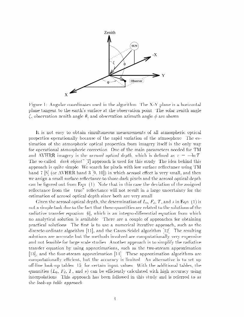
Atmospheric correction algorithms basically consist of two major steps. First, theoptical characteristics of the atmosphere are estimated either by using special featuresof the ground surface or by direct measurements of the atmospheric constituents [10]or by using theoretical models. Various quantities related to the atmospheric correc-tion can then be computed by the radiative transfer algorithms given the atmosphericoptical properties. Second, the remotely sensed imagery can be corrected by inversionprocedures that derive the surface re ectance, as we will shortly discussed in moredetails.In this paper, we will focus on the second step, describing our work on improvingthe computational e�ciency of the existing atmospheric correction algorithms. InSection 2, we present background material, while a known atmospheric correctionalgorithm is described in Section 3. We describe in Section 4 a substantially moree�cient version of the algorithm. In Section 5, we develop a parallel implementationof our algorithm, that is scalable in terms of number of processors, internal memorysize, and number of I/O nodes. A case study is presented in Section 6 and concludingremarks are given in Section 7.2 Background2.1 Atmospheric CorrectionIn order to correct for the atmospheric e�ects, the relationship between the upwardradiance Lm measured by the satellite and the surface re ectance � has to be estab-lished. The radiative transfer theory is used for this purpose. Assuming that theatmosphere is bounded by a Lambertian surface (i.e., re ects solar energy isotropi-cally), the upward radiance at the top of the cloud-free, horizontally homogeneousatmosphere can be expressed by [6] :Lm = L0 + �FdT�(1� s�) ; (1)where L0 is the upward radiance of the atmosphere with zero surface re ectance,often called path radiance, Fd is the downward ux (total integrated irradiance) atthe ground, T is the transmittance from the surface to the sensor (the probabilitythat a photon travels through a path without being scattered or absorbed), and sis the atmospheric albedo (the probability that a photon re ected from the surfaceis re ected back to the surface). From Eqn. (1) we can see that the factor �1�s� isthe sum of the in�nite series of interactions between the surface and the atmospherePn (s�)n.In order to invert � from Lm through Eqn. (1) , we need to determine the quantitiesL0, Fd, T , and s which are functions of the wavelength, atmospheric optical properties,and a set of locational parameters. The locational information includes, surface leveland observer heights, observation and solar zenith angles, and observation azimuthangle (Figure 1). There are two main tasks involved. The �rst is to estimate theatmospheric properties and the second is to calculate the functions required to invertthe surface re ectance �. 3

SUN

Zenith

X

-X

YObserverφ

θζFigure 1: Angular coordinates used in the algorithm. The X-Y plane is a horizontalplane tangent to the earth's surface at the observation point. The solar zenith angle�, observation zenith angle �, and observation azimuth angle � are shown.It is not easy to obtain simultaneous measurements of all atmospheric opticalproperties operationally because of the rapid variation of the atmosphere. The es-timation of the atmospheric optical properties from imagery itself is the only wayfor operational atmospheric correction. One of the main parameters needed for TMand AVHRR imagery is the aerosol optical depth, which is de�ned as � = � lnT .The so-called \dark object" [7] approach is used for this study. The idea behind thisapproach is quite simple. We search for pixels with low surface re ectance using TMband 7 [8] (or AVHRR band 3 [9, 10]) in which aerosol e�ect is very small, and thenwe assign a small surface re ectance to those dark pixels and the aerosol optical depthcan be �gured out from Eqn. (1). Note that in this case the deviation of the assignedre ectance from the \true" re ectance will not result in a large uncertainty for theestimation of aerosol optical depth since both are very small.Given the aerosol optical depth, the determination of L0, Fd, T , and s in Eqn. (1) isnot a simple task due to the fact that these quantities are related to the solutions of theradiative transfer equation [6], which is an integro-di�erential equation from whichno analytical solution is available. There are a couple of approaches for obtainingpractical solutions. The �rst is to use a numerical iterative approach, such as thediscrete-ordinate algorithm [11], and the Gauss-Seidel algorithm [12]. The resultingsolutions are accurate but the methods involved are computationally very expensiveand not feasible for large scale studies. Another approach is to simplify the radiativetransfer equation by using approximations, such as the two-stream approximation[13], and the four-stream approximation [14]. These approximation algorithms arecomputationally e�cient, but the accuracy is limited. An alternative is to set upo�-line look-up tables [15] for certain input values. With the additional tables, thequantities (L0, Fd, T , and s) can be e�ciently calculated with high accuracy usinginterpolations. This approach has been followed in this study and is referred to asthe look-up table approach. 4

2.2 Why High Performance Computing (HPC)?The existing code [15] for atmospheric correction based on the look-up table approachprocesses one pixel at a time (and meant to be used interactively), and takes 2.63seconds to correct a single pixel on a SPARC-10 machine, excluding I/O. A singleTM image that covers an area of size 180Km� 180Km consists of approximately 36million pixels per band, and will therefore require more than 15 years to correct withthe existing code, excluding the I/O time. We address this apparent intractability byattempting to achieve the following two objectives:� Minimize the overall computational complexity while maintaining the accuracyof the algorithm.� Maximize the scalability of the computation and the I/O as a function of theavailable resources (computation nodes, I/O nodes, and size of internal mem-ory).We believe that our algorithm, to be described in the rest of this paper, achievesboth objectives simultaneously. In fact, we are able to correct a TM image in lessthan 13 minutes on SPARC-10 (excluding I/O) and in less than 4.3 minutes on a32-processor CM-5 (including I/O).2.3 Data SourcesIn our studies, TM and AVHRR are used as the primary sources of input data to ouralgorithm. The essential features of these imagery types are as follows.The TM imagery consists of 7 channels that correspond to 7 spectral bands. Theresolution is 30m and �ve bands need to be corrected (band 6 corresponds to thethermal channel and the atmosphere does not have much scattering e�ect on band 7)[16]. An image covers approximately an area of size 180Km � 180Km and requires36MB per channel.The Path�nder AVHRR imagery consists of 12 channels from which only 5 chan-nels are original band information and only 2 bands need to be corrected [17]. Theremaining channels provide location, quality , cloud, and time information. Eachband requires about 20MB and the resolution is 8Km. Each AVHRR image coversthe entire globe.3 Atmospheric Correction Algorithm3.1 Description of AlgorithmA direct implementation of an atmospheric correction algorithm based on the look-up table approach has been described in [15], where a Fortran version is given. Theoverall algorithm can be sketched as follows.Algorithm (Atmospheric Correction)5

Input: N pixel values with the following information for each pixel: measurementwavelength, atmospheric correction parameters, location information and theday of measurement. Moreover, look-up tables for solar ux and for the func-tions L0, Fd, T and s are provided.Output: The surface re ectance at each pixel.for each pixel do:Step A: Read input parameters and appropriate look-up tables.Step B: Perform initializations and required normalizations.Step C: Compute L0, Fd, T and s by interpolation, using the look-up tables.Step D: Compute the surface re ectance � using Eqn. (1).endIn step B, we compute the solar ux for the measured wavelength by linear inter-polation (using the spectral irradiances and earth-sun distance for given wavelengths).Then we correct the solar ux for the day of the year for which the measurement ismade and we use the result to convert the measured radiance Lm from absolute unitsto re ectance units. We also compute the default values of the water and gaseous(carbon-dioxide and ozone) absorption by linear interpolation of the measured wave-length.All the interpolations in step B are spline interpolations of degree one. A splineinterpolation consists of polynomial pieces on subintervals joined together with certaincontinuity conditions. Formally, suppose that a table of n + 1 data points (xi; yi) isgiven, where 0 � i � n and x0 < x1 < : : : < xn is satis�ed. A spline function ofdegree k on these n + 1 points is a function, S such that, (1) S(xi) = yi, (2) on eachinterval [xi; xi+1), S is a polynomial of degree� k, and (3) S has a continuous (k�1)stderivative on [x0; xn]. Thus the spline interpolation of degree one is a piecewise linearfunction. By interpolating at a point x, we want to �nd y, the value of function S atpoint x, assuming that x0 � x � xn. Hence, for a spline interpolation of degree one,we need to �nd an index 0 � j < n such that xj � x � xj+1 and approximate thevalue y by yj + yj�yj+1xj�xj+1 (x� xj).Step C is computationally intensive and involves both linear and nonlinear in-terpolations. We give next the details of step C for computing L0, a function ofwavelength, location, and atmospheric parameters.Algorithm (Interpolate L0)Input: Wavelength, atmospheric correction parameters, location information andlook-up tables.begin 6

1. Interpolate L0 for the measured height.2. Interpolate L0 for the wavelength and adjust for the excess and de�cit of gaseousand water absorption.3. Interpolate L0 on measured solar zenith angle.4. Interpolate L0 on measured observation azimuth angle.5. Interpolate L0 on measured observation zenith angle.6. Interpolate L0 on measured optical thickness.endIn step 1, linear interpolations and extrapolations are performed. The interpola-tions in step 2 are piecewise exponential interpolations and those required by steps3, 4, and 5 are spline interpolations of degree one. For piecewise exponential inter-polation at a point x, xj � x < xj+1, y = e(� logyj+(1��) logyj+1) where, � = log( xxj+1 )log( xjxj+1 ).The interpolation on measured optical thickness required by Step 6 is non-linear andconsists of the following substeps. First we �nd the minimum of a non-linear func-tion over a subinterval; a costly process given the complexity of the function to beminimized. Second, we perform a linear or a nonlinear interpolation depending onthe outcome of the �rst substep.3.2 ImplementationThe direct atmospheric correction algorithm has been coded in Fortran [15] and testedon about 20 pixels. It uses eight look-up tables, one table for each of the 2 AVHRRbands of 0.639 and 0.845 �m and one for each of the 6 TM bands of 0.486, 0.587,0.663, 0.837, 1.663 and 2.189 �m. Each table contains the values of L0, Fd, T ands for nine solar zenith angles (10,20,30,40,50,60,66,72,and 78 degree), 13 observationzenith angles (0 to 78 degree, every 6 degree), 19 observation azimuth angles(0 to 180degree, every 10 degree, plus 5 and 175 degrees), 4 aerosol optical thicknesses (0.0,0.25, 0.50, and 1.0), and 3 observation heights (0.45, 4.5, and 80.0 kilometers). Onemore table is used which gives the solar spectral irradiances for 60 wavelengths in therange 0.486 to 2.189 �m.The code corrects single pixels of an image. The wavelength, solar and observationangles, and aerosol optical thickness data are assumed to be in the range discussedabove as no extrapolation is performed. If any of the selected parameters does notmatch any of the values used to construct the look-up tables, the algorithm inter-polates on that parameter. For observation height, the algorithm both interpolatesand extrapolates, and chooses the one that shows minimal atmospheric e�ect (lowervalues of intensity and higher values of transmittance are selected).The computation for each pixel begins by reading the input data and look-uptables, followed by approximating the values of L0, Fd, T and s by interpolations.Finally the surface re ectance of that pixel is computed using Eqn. (1).7

The resulting algorithm takes 2.63 seconds to correct a single pixel on a SPARC-10 system. Hence this code is not suitable for handling images as a single TM imagethat covers an area of size (180km � 180km) will take more than 15 years to correctall 5 bands. In the next section, we present our modi�ed version of the algorithmwhich runs substantially faster and is quite e�cient for handling images.4 Optimizing Overall Computational ComplexityWe introduce a number of techniques that lead to a substantially more e�cient versionof the atmospheric correction algorithm. We group our new techniques into 5 majortypes described brie y next.Reordering and Classifying Operations. In the previous algorithm, all opera-tions are repeated for each pixel. We rearrange the operations into three groups (1)image based, (2) window based, and (3) pixel based. The �rst group includes theoperations that are independent of pixel values. For example, reading the look-uptables, the initializations and the interpolations based on the height of the sensor areimage based operations. The corresponding operations can be performed for one pixeland used for all the remaining pixels. The second class of operations, window based,are reserved for those that depend on parameters which remain fairly constant over awindow of size w�w for a suitable value of w. For example, the aerosol optical thick-ness remains fairly constant over a small neighborhood. Atmospheric conditions andthe resolution of the image determine the value of w. It follows that the computationsand the interpolations belonging to the second group depend only on parameters thatcan be considered constant over windows. These operations can be performed onlyonce for each window if they are performed before any pixel based computation. Theremaining computations and interpolations belong to the third group and depend onpixel values or some other parameters that are di�erent for each pixel. We reorga-nized the operations of the atmospheric correction algorithm, so that the �rst group(image based) operations appear �rst followed by those of the second group (windowbased), and then by the third group operations. This has resulted in a substantialreduction of the total number of operations used.Performing Interpolations on Sub-cubes for Each Group. In the original al-gorithm, each interpolation causes one of the dimensions to be removed. Moreover,all the interpolations are piecewise interpolations. To reduce the number of oper-ations, we �rst identify the appropriate indexes along all the dimensions for whichinterpolations are required within a certain class (image, window, or pixel). Then weextract the sub-cube, obtained from the intersection of those indexes. With this tech-nique not only is the computational complexity reduced, but also the computationalcomplexity becomes almost independent of the size of the look-up tables.Data Dependent Control. Another technique is to use the characteristics of di�er-ent data inputs to reduce the overall computational complexity. For high resolutiondata most of the parameters are constant for the whole image while for coarse datamost parameters change from window (pixel) to window (pixel). On the other hand,8

the computational complexity per pixel is much more important for high resolutiondata than for coarse data due to the large di�erence in the amount of data involved.Changing Nonlinear Interpolations to Linear Interpolations. We have re-placed some of the nonlinear interpolations by linear interpolations at the expenseof increasing the sizes of the look-up tables. This technique decreases the numberof computations because those nonlinear interpolations are window based operationsand increasing the look-up table size mostly a�ects image based operations. For ex-ample, we replaced the nonlinear interpolations on measured optical thickness, whichinduce window based operations, with linear interpolations.Removing Unnecessary Interpolations. We replaced the interpolations withsimpler operations whenever possible. For example, since we are only dealing withsatellite images, we do not need to do the interpolation for the observation heightsince it can be assumed as constant.These techniques were quite e�ective in improving the performance while pre-serving the quality of the corrected imagery. Table 1 shows the performance of ouratmospheric correction algorithm, for di�erent window sizes and for di�erent typesof input data. The execution times do not include I/O time and are obtained on aSPARC-10 machine. Clearly, the new code is substantially faster than the code in[15] and can be used to correct all 5 bands of a TM image covering an area of size180km�180km with a window size of 19�19 in less than 13 minutes on a SPARC-10machine (excluding I/O).Data Type Window Size Time(�sec/pixel)TM 1 � 1 22:95TM 3 � 3 7:00TM 5 � 5 4:08TM 19 � 19 4:01TM 99 � 99 3:94AVHRR 1 � 1 527:50AVHRR 3 � 3 75:35AVHRR 5 � 5 35:76AVHRR 19 � 19 15:25Table 1: Performance on a SPARC-10 machine.It is interesting to notice that substantial speedups are achieved by increasing thewindow size up to a certain point. After that point (5�5 for TM), the speedups startto level o�. Also, the TM data is corrected much faster than AVHRR data by ouralgorithm for the following reasons. First, most of the computations for TM are imagebased operations while in AVHRR they are mostly window based operations. Second,9

we can skip some of the interpolations for TM data, such as those for observationangles.It should be mentioned that the input for our code is raw data and does not needany preprocessing, while the input for the code [15] is formatted and needs anotherprogram to transform the raw data into the special formatted input.5 Parallel implementationAtmospheric correction of global data sets requires the extensive handling of largeamounts of data residing in external storage, and hence the optimization of the I/Otime must be considered in addition to the computation time. We seek to achievean e�cient layout of the input imagery on the disks and an e�cient mapping of thecomputation across the processors in such a way the total computation and I/O timeis minimized. We concentrate �rst on modeling the I/O performance; we then give adescription of the parallel algorithm together with its overall theoretical performancefollowed by experimental results on a 32-node CM-5.Interconnection Network

IOP IOPIOP

PN PN PN

Figure 2: Processing nodes and I/O nodes are connected by an interconnection net-work.5.1 I/O ModelOur parallel model consists of a number p of computation nodes P0, P1, : : :, Pp�1and a number d of I/O nodes, N0, N1, : : :, Nd�1, connected by an interconnectionnetwork (Figure 2). For our purposes, we view each I/O node as holding a largedisk (or a disk array). Data are transferred into and out of external storage in unitsof blocks, each block consisting of a number b of contiguous records. Each of the d10

disks can simultaneously transfer a block into the network. Therefore the theoreticaltotal I/O bandwidth is d times the bandwidth provided by a single I/O node. Theactual bandwidth depends on several factors including the interconnection network,the ratio of p and d, and the network I/O interface.Most current parallel systems use the technique of disk striping in which con-secutive blocks are stored on di�erent disks. For our case, an n � n image (say, inrow-major order form) will be striped across the d disks in block units. When theimage is accessed in parallel, we can adopt the single disk model with a very largebandwidth. In the single disk model, the time to transfer data is the sum of twocomponents ta + Nd te, where ta is the access setup time, N the data size, and te thetransfer time per element. Thus the I/O time depends essentially on the two param-eters, ta and te. On a serial machine, the access setup time is mostly the seek time tswhich is around 20msec but on parallel machines it is considerably larger, whereasthe transfer time per element is substantially smaller (inverse of total bandwidth).In spite of the fact that ta and te vary from one application to another, they can beapproximated reasonably well by constants.The I/O performance can be estimated by using the number np of passes throughthe data and the number na of disk accesses. In this case, the total data transfertime is given by (na� ta) + (np�N � te). Since the access setup time is much largerthan the transfer time, minimizing the number of disk accesses is usually much moreimportant than minimizing the number of passes. For our implementation of theatmospheric correction algorithm to be discussed shortly, it is possible to minimizethe I/O time by minimizing both parameters independently. For other problems (e.g.,matrix transposition), it is possible to come up with algorithms that use more passesbut requires less total I/O time by reducing the number of disk accesses [18]. A briefdescription of the CM-5 I/O system and its relationship to our model is presented inAppendix A.5.2 Parallel AlgorithmWe now sketch our parallel atmospheric correction algorithm and how it achieves itscomputation and I/O scalability. The algorithm is designed in the Single ProgramMultiple Data (SPMD) model using the multiblock PARTI library. Therefore eachprocessor runs the same code but on di�erent parts of the image. The MultiblockPARTI library [19, 20] is a runtime support library for parallelizing application codese�ciently which provides a shared memory view on distributed memory machines.This makes our code portable to a large set of parallel machines since the library isavailable on the CM-5, the Intel iPSC/860 and Paragon, the IBM SP-1 and the PVMmessage passing environment for networks of workstations.A straightforward parallel implementation of the algorithm applied to each bandof a N � N image4 requires only one pass through the image and can be done asfollows. We read a block of maximum possible size, (say n � n) of the image thatcan �t in the internal memory with corresponding parameters for that part of the4Here we have assumed that the numbers of columns and rows are equal for simplicity. The sametype of analysis can be carried out in the more general case.11

image. We apply our atmospheric correction procedure on the current block andwrite back the results. The procedure is repeated until the entire image is processed.This method requires n disk accesses per iteration, and hence Cn N2MP � C N2pM P diskaccesses per band are required, where M is the memory size per processor and C issome constant. However we can modify the algorithm to minimize the number of diskaccesses as follows. During each iteration, instead of reading a block, we read a slabconsisting of the maximum possible number (say r) of consecutive rows of the imagethat can �t in the internal memory with corresponding parameters. We apply theatmospheric correction procedure on the slab and write back the results and repeatthe procedure until the entire image is processed. Now we need only one disk accessper iteration and hence the total number of disk accesses is reduced to C N2MP whichis clearly optimal. The new algorithm still requires only one pass through the imageand therefore the total transfer time is also optimal and is given byTI=O � bN2fC1 taMp + C2 ted gwhere b is the number of bands that we correct (b = 5 for TM and b = 2 for AVHRR),C1 is the cost of constant number of disk accesses per pass, and C2 is the numberof bytes per pixel that we read or write. Given these relations, the I/O time can becontrolled by changing the number of processors and the number of disk I/O nodes.In our algorithm, interprocessor communication is only introduced by the possi-bility of partitioning windows across processors. This can be eliminated by replacingr with r0 = b rw:pc � w � p. This can be done only if at least w rows can �t in theinternal memory of each processor, which is a realistic assumption for all reasonablevalues of w (i.e. � 500).The computation time for both TM and AVHRR can be estimated byTcomp � bfC3 + C4 N2pw2 + C5N2p g;where C3, C4 and C5 are some machine dependent constants. In fact C3 is the requiredtime for image based computations, C4 is the required time per window for windowbased operations and C5 is the required time per pixel for pixel based operations.These constants can be accurately estimated for a given machine. As an example,for TM data on CM-5, C3 � 26sec, C4 � 62�sec, and C5 � 18�sec. Note that C3includes the I/O time for reading all the look-up tables. These numbers are valid forlarge data and agree with the observed experimental results.Summarizing , the total time is given byTtotal � bfC3 + C4 N2w2p + C5N2p + C1 N2Mpta + C2N2d tegThe above performance analysis indicate that our algorithm is scalable in terms ofthe parameters p, M , and d because for each term with N in the numerator we havep, M , or d in the denominator. Also, for a desired value of Ttotal, we can derive thenumber of processors and the number d of disk I/O nodes to achieve this.12

0 100 200 300 400 500 600 700 800 900 10000

500

1000

1500

2000

2500

3000

Image Size (M Pixel)

TIM

E (

sec)

W=5X5 (32P)

W=5X5 (16P)

W=1X1 (32P)

Figure 3: Atmospheric correction performance of TM imagery on CM-5, for di�erentimage sizes, two window sizes, and a di�erent number of processors.The results of running our code on a 32-node CM-5 are illustrated in Figure 3.The �gure shows the total time in seconds for di�erent image sizes, two window sizesand a di�erent number of processors. We have used the least squares approximationto smooth the curves, but we have also included the real data for one of the cases(w = 5 � 5 on 16 processors) to show the linearity of the experimental data. Theseexperimental results are consistent with the analysis carried out in our model. Fromthe graph, the running time scales properly with the image size and with the numberof processors for di�erent window sizes.6 Case StudyThe application of our algorithm on a real TM imagery is presented in this section.Figure 4 shows a subset of TM image bands 1, 3, and 7 acquired on Aug. 17, 1989in Amazon Basin area. As we can see, a large portion of the image in bands 1and 3 in the middle is occupied by hazy aerosols and thin clouds but band 7 is lesscontaminated because it is in large wavelengths and scattering e�ect is negligible. Inorder to remove the aerosol contamination, the �rst step is to implement the so-called"dark-object" approach to estimate aerosol optical depth using band 7. We developeda preliminary program which estimates the aerosol optical depth for TM images andapplied it to the mentioned image 5.After having obtained aerosol optical depth for each channel, the surface re- ectance is retrieved using the new atmospheric correction algorithm described inSection 5. The retrieved re ectance is shown in Figure 4. It is evident that most ofhazy aerosols in channels 1 and 3 have been removed. Also it is interesting to seethat the corrected channel 3 looks even more clear than channel 7. The retrieved5Details of this algorithm will be published after validation.13

Band 1, Before Correction Band 1, After CorrectionBand 3, Before Correction Band 3, After Correction

Band 7Figure 4: TM imagery (512 � 512).14

surface re ectance underneath the hazy aerosols will be further evaluated with theknowledge of the ground truth.7 ConclusionWe have introduced a number of techniques to obtain a very e�cient atmosphericcorrection algorithm based on the look-up table approach. As a result our algorithmcan correct all 5 bands of a TM image, covering an area of size 180km � 180km,in less than 13 minutes on a SPARC-10 machine (excluding I/O). A parallel versionof the algorithm that is scalable in terms of the number of processors, the numberof I/O nodes, and the size of internal memory, was also described and analyzed.Experimental results on a 32-node CM-5 machine are provided.This work constitutes a part of a large multidisciplinary grand challenge project onapplying high performance computing to land cover dynamics. Other aspects includeparallel algorithms and systems for image processing and spatial data handling withemphasis on object oriented programming and parallel I/O of large scale images andmaps.AcknowledgmentWe thank Dr. Alan Sussman for helping us in using multiblock PARTI library. Ms.Shana Mattoo provided the original NASA code described in [15] and have answeredmany of our questions regarding the atmospheric correction algorithm based on look-up tables. Her help is greatly appreciated. Also, thanks to Professor Ralph Dubayahfor providing comments regarding this project.References[1] C. O. Justice, J. R. G. Townshend, and V. T. Kalb, Representation of vegetationby continental data set derived from NOAA-AVHRR data, International Journalof Remote Sensing, 1991, 12:999-1021.[2] J. R. G. Townshend, Global datasets for land applications from the Advanced VeryHigh Resolution Radiometer: an introduction, International Journal of RemoteSensing, 1994, 15:3319-3332.[3] Y. J. Kaufman, The atmospheric e�ect on remote sensing and its correction,Chapter 9 in Optical Remote Sensing, technology and application, G. Asrar,Ed., Wiley, 1989.[4] R. S. Fraser and Y. J. Kaufman, The relative importance of scattering and ab-sorption in remote sensing, IEEE Trans. Geosciences and Remote Sensing, 1985,23:625-633. 15

[5] R. S. Fraser, O. P. Bahethi, and A. H. Al-Abbas, The e�ect of the atmosphere onclassi�cation of satellite observations to identify surface features, Remote Sens.Environment, 1977, 6:229.[6] S. Chandrasekar, Radiative Transfer, London: Oxford University Press, 1960.[7] Y. J. Kaufman and C. Sendra, Automatic atmospheric correction, Intl. Journalof Remote sensing, 1988, 9:1357-1381.[8] Y. J. Kaufman, L. A. Lorraine, B. C. Gao, and R. R. Li, Remote sensing ofaerosol over the continents: Dark targets identi�ed by the 2.2 um channel, inpreparation, 1995.[9] B. N. Holben, E. Vermote, Y. J. Kaufman, D. Tanre, V. kalb, Aerosols retrievalover land from AVHRR data - Application for atmospheric correction, IEEETrans. Geosci. Remote Sens., 1992, 30:212-222.[10] Y. J. Kaufman, A. Gitelson, A. Karnieli, E. Ganor, R. S. Fraser, T. Nakajima,S. Mattoo, and B. N. Holben, Size distribution and scattering phase function ofaerosol particles retrieved from sky brightness measurements, JGR-Atmospheres,1994, 99:10341-10356.[11] J. Lenoble, Radiative Transfer in Scattering and Absorbing Atmospheres: Stan-dard Computational Procedures, A. Deepak Publ., Hampton, Virginia, 1985.[12] S. Liang and A. H. Strahler, Calculation of the angular radiance distributionfor a coupled atmosphere and canopy, IEEE Trans. Geosci. Remote Sens., 1993,31:491-502.[13] W. E. Meador and W. R. Weaver, Two-stream approximations to radiative trans-fer in planetary atmospheres: A uni�ed description of existing methods and a newimprovement, J. Atmos. Sci., 1980, 37:630-643.[14] S. Liang and A. H. Strahler, Four-stream solution for atmosphere radiative trans-fer over an non-Lambertian surface, Appl. Opt., 1994, 33:5745-5753.[15] R. S. Fraser, R. A. Ferrare, Y. J. Kaufman, B. L. Markham, and S. Mattoo, Algo-rithm for atmospheric corrections of aircraft and satellite imagery, Intl. Journalof Remote sensing, 1992, 13:541-557.[16] J. R. G. Townshend, J. Cushnie, J. R. Hardy, and A. Wilson, Thematic Mapperdata: Characteristics and use, 1983.[17] J. R. G. Townshend, M. E. James, S. Liang, and S. Goward, A long term dataset for global terrestrial observations: Report of the AVHRR Path�nder LandScience Working Group, NASA-TM, in press, 1995.[18] S. D.Kaushik, C.-H. Huang, J. R. Johnson, R. W. Johnson, P. Sadayappan,E�cient Transposition algorithms for large Matrices, ACM, 1993.16

[19] G. Agrawal, A. Sussman, and J. Saltz, Compiler and runtime support for struc-tured and block structured applications, In Proceedings Supercomputing '93,IEEE Computer Society Press, November 1993.[20] A. Sussman and J. Saltz, A manual for the multiblock PARTI runtime primitivesversion 4, Technical Report CS-TR-3070 and UMIACS-TR-93-36, University ofMaryland, May 1993.[21] CM-5 I/O System Programming Guide, Version 7.2, Thinking Machines Corpo-ration, Cambridge,MA, September 1993.[22] Connection Machine CM-5 Technical Summary, Technical report, Thinking Ma-chines Corporation, Cambridge,MA, October 1991.[23] C. E. Leiserson, Z. S. Abuhamdeh, D. C. Douglas, C. R. Feynman, M. N. Gan-mukhi, J. V. Hill, W. D. Hillis, B. C. Kuszmaul, M. A. St. Pierre, D. S. Wells,M. C. Wong, S. W. Yang, and R. Zak, The Network Architecture of the Con-nection Machine CM-5, Extended Abstract, Thinking Machines Corporation,Cambridge,MA, July 1992.

17

P P P P P P CP CP I/O I/O

NI NI NI NI NI NI NI NI NI NI

Data Network

Control Network

Dia

gnos

tic

Net

wor

k

Control I/OInterfacesProcessors

Processing NodesFigure 5: The organization of the Connection Machine CM-5. The machine has threenetworks: a data network, a control network, and a diagnostic network.The dataand control networks are connected to processing nodes, control processors, and I/Ochannels via a network interface.A CM-5 I/O SystemHere we examine brie y the CM-5 I/O system and how it relates to our model[21, 22, 23]. The CM-5 contains three communication networks (Figure 5): a datanetwork, a control network and a diagnostic network. The processing nodes (PNs),the control processors and the I/O nodes are interconnected by the three networks.The data network provides high-performance point-to-point data communicationsbetween system components whereas the control network provides cooperative andsystem management operations. The diagnostic network allows back-door access toall system hardware to test system integrity and to detect and isolate errors. TheScalable Disk Array (SDA) provides striping across all the disks and communicateswith the processors via the data network using high-bandwidth I/O interfaces. Abasic read or write operation consists of two phases. A read's two phases are:� Raw data transfer: transferring data between the disks and the PNs' user mem-ory. The transfer rate of this phase is usually dominated by the speed of theSDA unless the number of processing nodes is small compared to the numberof disks.� Data routing: Reordering the data in PN memory so that every PN has thecorrect data in the correct order for the application. The performance of thisphase depends on several factors such as (1) the number of processing nodes,(2) the application's geometry, and (3) the number of bytes per shape positionor array element.In general data is stored in serial order on the SDA. When we read a �le, data isread as fast as possible during the �rst phase and sent to the PNs in such a way as tomake optimal use of the Data Network. In the second phase, the data is parallelized18

according to the speci�ed shape and routed to the correct locations. In the writeoperation we have the two phases in reverse order. It can be shown that the timefor the second phase is much smaller than the time for the �rst phase, and hence oursingle disk model works well for the CM-5. We measured the ta and te on a 32 nodeCM-5 with two I/O nodes and the results are shown in table 2.OPERATION SHAPE ta(msec) te(microsec)READ 1 DIMENSION 230 0.098READ 2 DIMENSION 217 0.160READ 3 DIMENSION 235 0.166WRITE 1 DIMENSION 700 0.212WRITE 2 DIMENSION 755 0.210WRITE 3 DIMENSION 757 0.214Table 2: ta and te for a 32 node CM-5.

19