DYNAMICS GROUP

Dynamics of StructuresArnaud Deraemaeker

1

Contents

1 Introduction 41.1 Mechanism of Vibrations . . . . . . . . . . . . . . . . . . . . . . . . . . .. . . . . 41.2 Sources of excitations . . . . . . . . . . . . . . . . . . . . . . . . . . . .. . . . . . 5

1.2.1 Free vibration . . . . . . . . . . . . . . . . . . . . . . . . . . . . . . . . .. 51.2.2 Forced vibrations . . . . . . . . . . . . . . . . . . . . . . . . . . . . . .. . 5

1.3 Vibration sources in civil engineering . . . . . . . . . . . . . .. . . . . . . . . . . 71.4 Positive vs negative effects of vibrations . . . . . . . . . . .. . . . . . . . . . . . . 91.5 A first feeling about vibrations through movies and experiments . . . . . . . . . . . 10

2 Tools to describe an deal with dynamic signals 102.1 Harmonic signals . . . . . . . . . . . . . . . . . . . . . . . . . . . . . . . . .. . . 102.2 Harmonic analysis: the discrete Fourier transform . . . .. . . . . . . . . . . . . . . 12

2.2.1 Amplitude and phase formulation . . . . . . . . . . . . . . . . . .. . . . . 142.2.2 Complex formulation . . . . . . . . . . . . . . . . . . . . . . . . . . . .. . 142.2.3 Examples of Fourier transforms of periodic signals . .. . . . . . . . . . . . 16

2.3 The continuous Fourier transform . . . . . . . . . . . . . . . . . . .. . . . . . . . 172.3.1 Examples of continuous Fourier transforms and properties . . . . . . . . . . 18

2.4 The convolution integral and the theorem of Parseval . . .. . . . . . . . . . . . . . 232.4.1 The convolution integral . . . . . . . . . . . . . . . . . . . . . . . .. . . . 232.4.2 The theorem of Parseval . . . . . . . . . . . . . . . . . . . . . . . . . .. . 26

3 Single degree of freedom system 273.1 One degree of freedom systems in real life . . . . . . . . . . . . .. . . . . . . . . . 273.2 Response of a single degree of freedom system without damping . . . . . . . . . . . 30

3.2.1 General solution of the equation of motion . . . . . . . . . .. . . . . . . . 313.2.2 Particular solution . . . . . . . . . . . . . . . . . . . . . . . . . . . .. . . 32

3.3 Response of a single degree of freedom system with damping . . . . . . . . . . . . . 353.3.1 General solution of the equation of motion . . . . . . . . . .. . . . . . . . 353.3.2 The impulse response . . . . . . . . . . . . . . . . . . . . . . . . . . . .. . 383.3.3 Particular solution of the equation of motion . . . . . . .. . . . . . . . . . 383.3.4 Duhamel’s integral . . . . . . . . . . . . . . . . . . . . . . . . . . . . .. . 413.3.5 Base excitation . . . . . . . . . . . . . . . . . . . . . . . . . . . . . . . .. 42

3.4 Reduction to a one dof system . . . . . . . . . . . . . . . . . . . . . . . .. . . . . 423.4.1 Equivalent stiffness . . . . . . . . . . . . . . . . . . . . . . . . . . .. . . . 433.4.2 Equivalent mass . . . . . . . . . . . . . . . . . . . . . . . . . . . . . . . .473.4.3 Equivalent damping . . . . . . . . . . . . . . . . . . . . . . . . . . . . .. 483.4.4 Reduction to a single dof system : limitations . . . . . . .. . . . . . . . . . 55

3.5 One DOF application: the accelerometer . . . . . . . . . . . . . .. . . . . . . . . . 56

4 Vibration isolation 584.1 Direct vibration isolation . . . . . . . . . . . . . . . . . . . . . . . .. . . . . . . . 584.2 Inverse vibration isolation . . . . . . . . . . . . . . . . . . . . . . .. . . . . . . . . 59

2

5 Multiple degree of freedom systems 625.1 Response of a multiple degrees of freedom system withoutdamping . . . . . . . . . 63

5.1.1 General solution of the equations of motion . . . . . . . . .. . . . . . . . . 635.1.2 Orthogonality of the mode shapes . . . . . . . . . . . . . . . . . .. . . . . 665.1.3 Particular solution of the equation of motion . . . . . . .. . . . . . . . . . 67

5.2 Response of a multiple degrees of freedom system with damping . . . . . . . . . . . 705.2.1 General solution of the equations of motion . . . . . . . . .. . . . . . . . . 715.2.2 Particular solution of the equations of motion . . . . . .. . . . . . . . . . . 71

5.3 MDOF application: the tuned mass damper . . . . . . . . . . . . . .. . . . . . . . 75

6 Continuous systems 846.1 Beams and bars . . . . . . . . . . . . . . . . . . . . . . . . . . . . . . . . . . . .. 84

6.1.1 Boundary conditions for beams and bars . . . . . . . . . . . . .. . . . . . . 846.1.2 Bar in traction: equation of motion . . . . . . . . . . . . . . . .. . . . . . . 856.1.3 Bar in traction: mode shapes and eigenfrequencies . . .. . . . . . . . . . . 856.1.4 Bar in traction: orthogonality conditions . . . . . . . . .. . . . . . . . . . . 876.1.5 Bar in traction: projection in the modal basis . . . . . . .. . . . . . . . . . 896.1.6 Bar in traction: particular solution . . . . . . . . . . . . . .. . . . . . . . . 906.1.7 Bar in traction: comparison with mdof systems . . . . . . .. . . . . . . . . 926.1.8 Beam in bending: equation of motion . . . . . . . . . . . . . . . .. . . . . 936.1.9 Beam in bending: mode shapes and eigenfrequencies . . .. . . . . . . . . . 936.1.10 Beam in bending: orthogonality conditions . . . . . . . .. . . . . . . . . . 996.1.11 Beam in bending: projection in the modal basis . . . . . .. . . . . . . . . . 101

6.2 Complex structures . . . . . . . . . . . . . . . . . . . . . . . . . . . . . . .. . . . 1016.2.1 Modeling of damping . . . . . . . . . . . . . . . . . . . . . . . . . . . . .. 1046.2.2 Tuned mass damper attached to continuous structures .. . . . . . . . . . . . 104

3

1 Introduction

Vibration refers to mechanical oscillations about an equilibrium point. The oscillations may be peri-odic such as the motion of a pendulum or random such as the movement of a tire on a gravel road. Inpractice, every object is subject to a certain level of vibration, which can often not be seen with thenaked eye. This does not mean that this phenomenon is not important, and it deserves, in many cases,to be studied. Examples of objects creating vibration in everyday life are a shaver, a vibrator in a cellphone, a loudspeaker, tools, rotating machines and vehicles in motion such as trains or trams.

1.1 Mechanism of Vibrations

The underlying mechanism of vibrations consists in the transfer of the potential energy into kineticenergy, and vice versa. Examples of the mass-spring system and the pendulum are illustrated inFigures 1 and 2.

mm

m

PE maxKE = 0

PE maxKE = 0

PE = 0KE max

KE Kinetic EnergyPE Potential Energy

Figure 1: Transfer of the potential energy to kinetic energyand vice versa in the mass-spring system

PE maxKE = 0

PE maxKE = 0

PE = 0KE max

KE Kinetic EnergyPE Potential Energy

Figure 2: Transfer of the potential energy to kinetic energyand vice versa in the pendulum

4

1.2 Sources of excitations

In order for a body to vibrate, it has to be excited by a source.The sources of excitation can bedivided in two main categories : free vibrations and forced vibrations. Free vibrations correspond tothe case where the vibration is caused by an initial source which is then removed so that the structurevibrates without any force acting on it. Forced vibrations correspond to the case where an excitationis permanently applied to the structure.

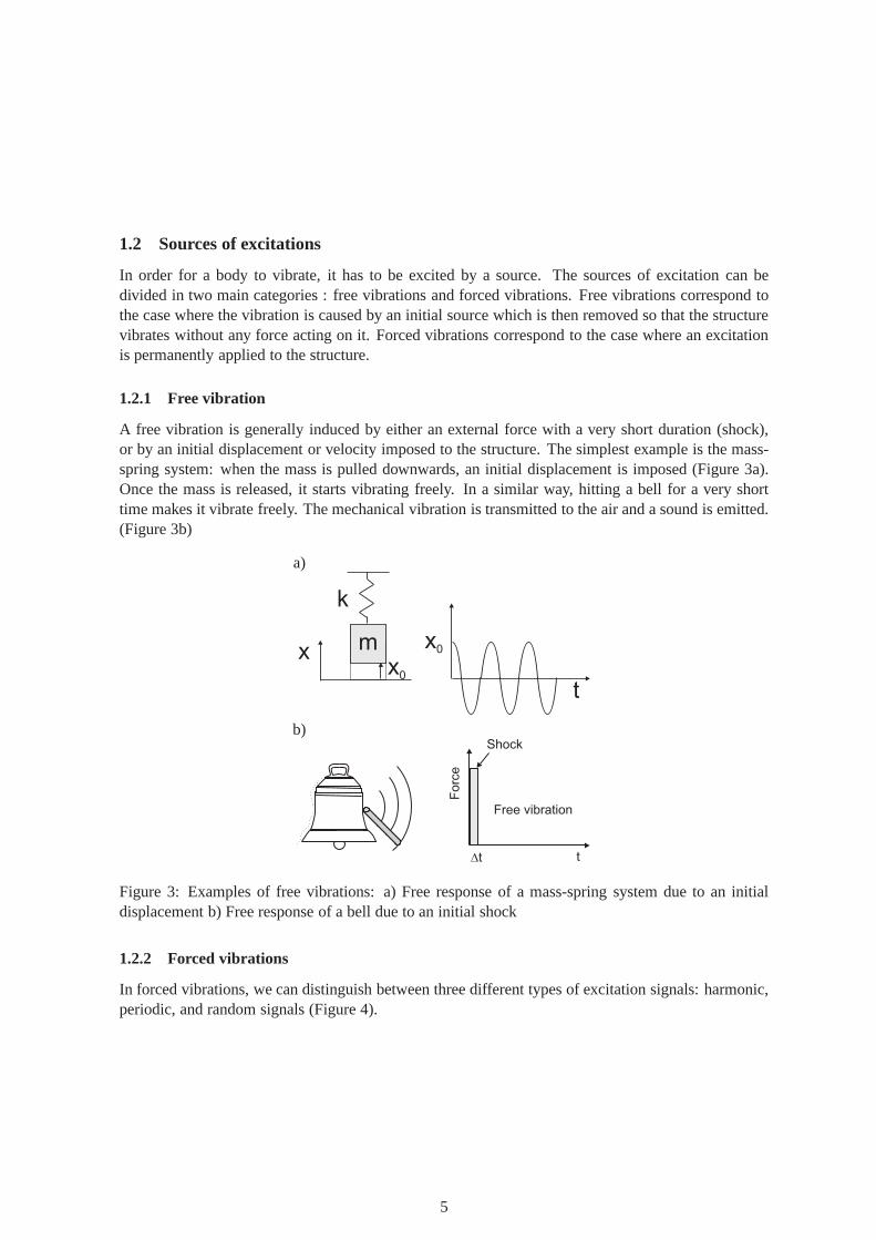
1.2.1 Free vibration

A free vibration is generally induced by either an external force with a very short duration (shock),or by an initial displacement or velocity imposed to the structure. The simplest example is the mass-spring system: when the mass is pulled downwards, an initialdisplacement is imposed (Figure 3a).Once the mass is released, it starts vibrating freely. In a similar way, hitting a bell for a very shorttime makes it vibrate freely. The mechanical vibration is transmitted to the air and a sound is emitted.(Figure 3b)

a)

k

mxx0

x0

t

b)

Dt t

Forc

e

Shock

Free vibration

Figure 3: Examples of free vibrations: a) Free response of a mass-spring system due to an initialdisplacement b) Free response of a bell due to an initial shock

1.2.2 Forced vibrations

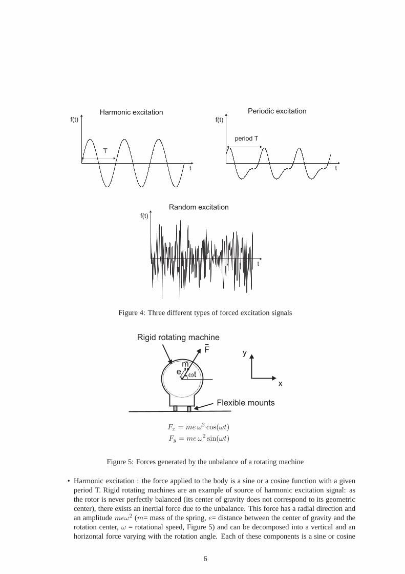
In forced vibrations, we can distinguish between three different types of excitation signals: harmonic,periodic, and random signals (Figure 4).

5

t

T

t

period T

f(t)f(t)

f(t)

t

Harmonic excitation Periodic excitation

Random excitation

Figure 4: Three different types of forced excitation signals

Flexible mounts

Rigid rotating machine

me

F

x

y

wt

Fx = meω2 cos(ωt)

Fy = meω2 sin(ωt)

Figure 5: Forces generated by the unbalance of a rotating machine

• Harmonic excitation : the force applied to the body is a sineor a cosine function with a givenperiod T. Rigid rotating machines are an example of source ofharmonic excitation signal: asthe rotor is never perfectly balanced (its center of gravitydoes not correspond to its geometriccenter), there exists an inertial force due to the unbalance. This force has a radial direction andan amplitudemeω2 (m= mass of the spring,e= distance between the center of gravity and therotation center,ω = rotational speed, Figure 5) and can be decomposed into a vertical and anhorizontal force varying with the rotation angle. Each of these components is a sine or cosine

6

function and is transmitted to the environment through the fixations of the rotating machine.This excitation is therefore periodic and harmonic.

• Periodic excitation: this corresponds to excitation signals which repeat themselves over timewith a certain period T. As an example, piston engines generate periodic excitation (the periodcorresponding to one full rotation of the crankshaft) whichis not made of a single sine or cosinecomponent (existence of harmonics of the fundamental frequency).

• Random excitation: a random excitation signal has no fundamental frequency and one cannotdistinguish a pattern which repeats itself over time. Examples are the forces generated by wind,earthquakes (Figure 6), traffic, waves etc.

Gro

und m

otion

Building

Time

Figure 6: Example of excitation signal induced by an earthquake on a building

1.3 Vibration sources in civil engineering

In civil engineering, one can distinguish between internaland external sources of vibrations:

• Internal sources:

– Ventilation systems

– Elevator and conveyance systems

– Fluid pumping equipment

– Machines and generators

– Aerobics and exercise rooms, human activity

• External sources:

– Seismic activity

– Subway, road and rail systems, airplanes

– Construction equipment

– Wind, Waves

Traditionally, vibrations have not been a big concern in civil engineering, except for high levelsof vibrations caused by earthquakes. In recent years however, the sources and levels of excitationshave increased, while at the same time the comfort demands are increasing and health issues areappearing. In some cases, novel high precision technologies require very low levels of vibrations.Another important change is the fact that new designs of structures make them more susceptible to

7

vibrations. For example, where in the past, bridges where massive structures, they tend to a more andmore slender design aimed at optimising the use of materials(Figure 7). The drawback is that such adesign makes them much more prone to vibrations. The use of novel materials such as composites isalso responsible for a lower level of damping, hence more vibrations.

Figure 7: Evolution in the design of bridges: from massive[http : //www.bridge2faith.net] toslender structures[https : //fr.wikipedia.org/wiki/V iaduc de Millau]

We detail here below a few examples of structures where vibrations are problematic:

• The Millenium Bridge (Figure 8) in London is a steel suspension bridge for pedestrians cross-ing the River Thames. During its opening in June 2000, it was subjected to very high levelsof lateral vibrations due to pedestrians walking on the bridge. The bridge was closed until asolution to the problem could be implemented.

• In cable-stayed bridges(Figure 8), wind excitation can cause excessive levels of vibrations inthe cables. Damping systems are often implemented in order to solve this problem.

• In high-rise buildings, wind excitation can cause an oscillatory motion which is detrimentalfor comfort of the inhabitants in the top levels. These structures are also more vulnerable toearthquake excitation. An example is the Taipei 101 (Figure9) building (509 m) in which amassive device called ”pendulum tuned mass damper” has beenimplemented. The device isdesigned to damp the vibrations due to earthquakes which could impact the structural integrityof the building.

• The originalTacoma Narrows bridge opened on July 1, 1940 and collapsed into the PugetSound in Pierce County, Washington on November 7 1940 (Figure 9). The collapse was due tohigh wind conditions which caused excessive vibrations leading to the collapse of the bridge.

8

Figure 8: The Millenium bridge[https : //fr.wikipedia.org/wiki/Millennium Bridge (Londres)]and a cable-stayed bridge (Dongting, China)[http : //sitesavisiter.com/pont − du − lac −dongting]

Figure 9: The Taipei building [http://blog.artnn.ru] and the original Tacoma Narrows bridge[http://www.maxisciences.com/construction/pont-de-tacoma-washington-1940art3460.html]

1.4 Positive vs negative effects of vibrations

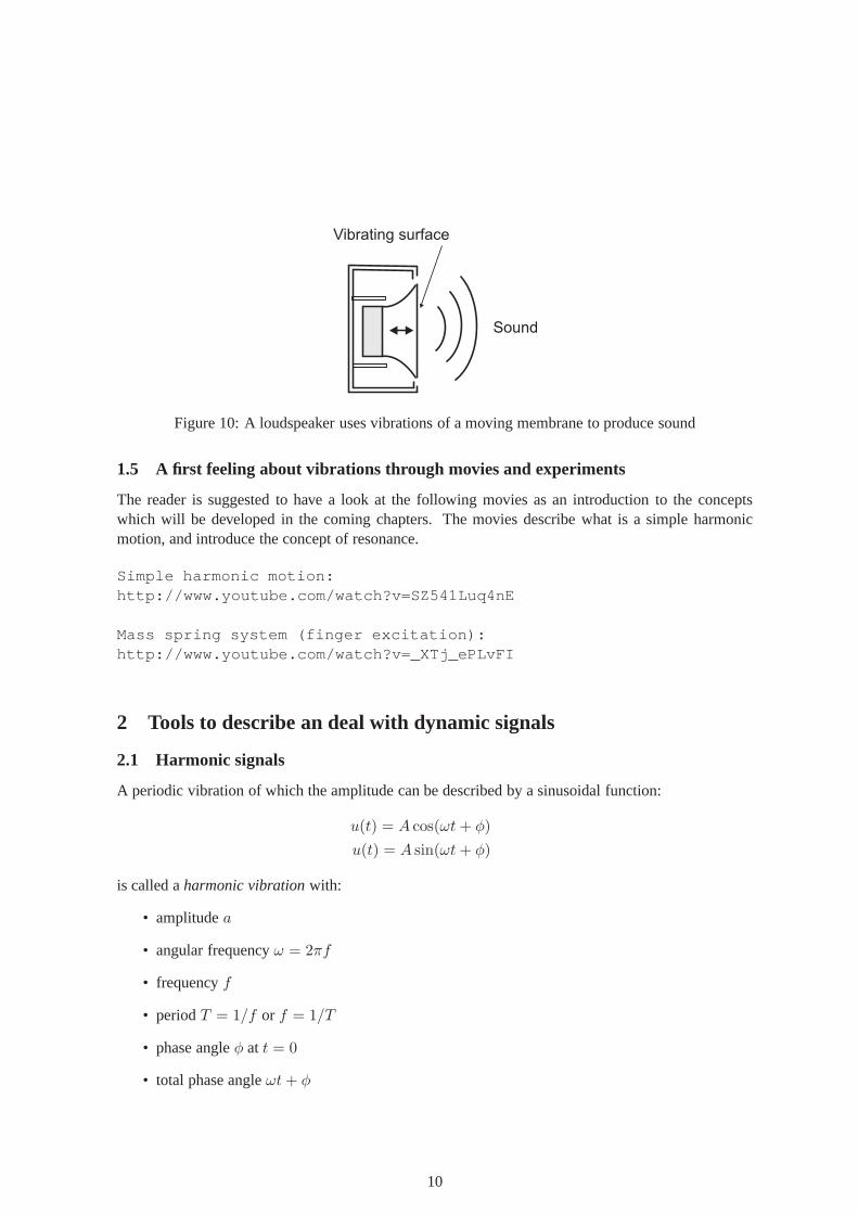
We have already listed negative aspects of vibrations: excessive levels of vibrations can cause fatigue,health and comfort issues, degrade the performance of systems and in the most catastrophic casecan lead to collapse. There are however some cases in which vibrations are useful, examples are aloudspeaker (Figure 10) which requires vibrations to produce sound, an electric toothbrush, a sander,musical instruments, etc. Another example is the use of high-frequency vibrations in formula oneengines to reduce the friction.

9

Vibrating surface

Sound

Figure 10: A loudspeaker uses vibrations of a moving membrane to produce sound

1.5 A first feeling about vibrations through movies and experiments

The reader is suggested to have a look at the following moviesas an introduction to the conceptswhich will be developed in the coming chapters. The movies describe what is a simple harmonicmotion, and introduce the concept of resonance.

Simple harmonic motion:http://www.youtube.com/watch?v=SZ541Luq4nE

Mass spring system (finger excitation):http://www.youtube.com/watch?v=_XTj_ePLvFI

2 Tools to describe an deal with dynamic signals

2.1 Harmonic signals

A periodic vibration of which the amplitude can be describedby a sinusoidal function:

u(t) = A cos(ωt+ φ)

u(t) = A sin(ωt+ φ)

is called aharmonic vibration with:

• amplitudea

• angular frequencyω = 2πf

• frequencyf

• periodT = 1/f or f = 1/T

• phase angleφ at t = 0

• total phase angleωt+ φ

10

Harmonic signals are more conveniently represented in the complex plane. In order to do that,one writes:

u(t) = aei(ωt+φ) = a cos(ωt+ φ) + i a sin(ωt+ φ)

which can be written:u(t) = aeiφeiωt = Aeiωt

whereA = aeiφ = a cos(φ) + ia sin(φ)

which introduces the complex amplitudeA which is independent of time (Figure 11). Note thatintroducing imaginary numbers is a kind of artefact: there exists no vibration which is imaginary, allvibration signals are real. The important point to rememberis that the complex amplitudeA carries theinformation of both the amplitudea and the phase angleφ and therefore contains all the informationabout the harmonic signal.

Re

Im

f

wt

u(t)

Aa

Figure 11: Representation of the harmonic signal as a complex numberA with a phase and amplitudein the complex plane

The use of the complex notation is particularly useful when one wishes to calculate the first andsecond derivatives of a harmonic signal with respect to time:

u(t) = Aeiωt

v(t) =du(t)

dt= iωAeiωt = iωu(t)

a(t) =d v(t)

dt= −ω2Aeiωt = −ω2u(t)

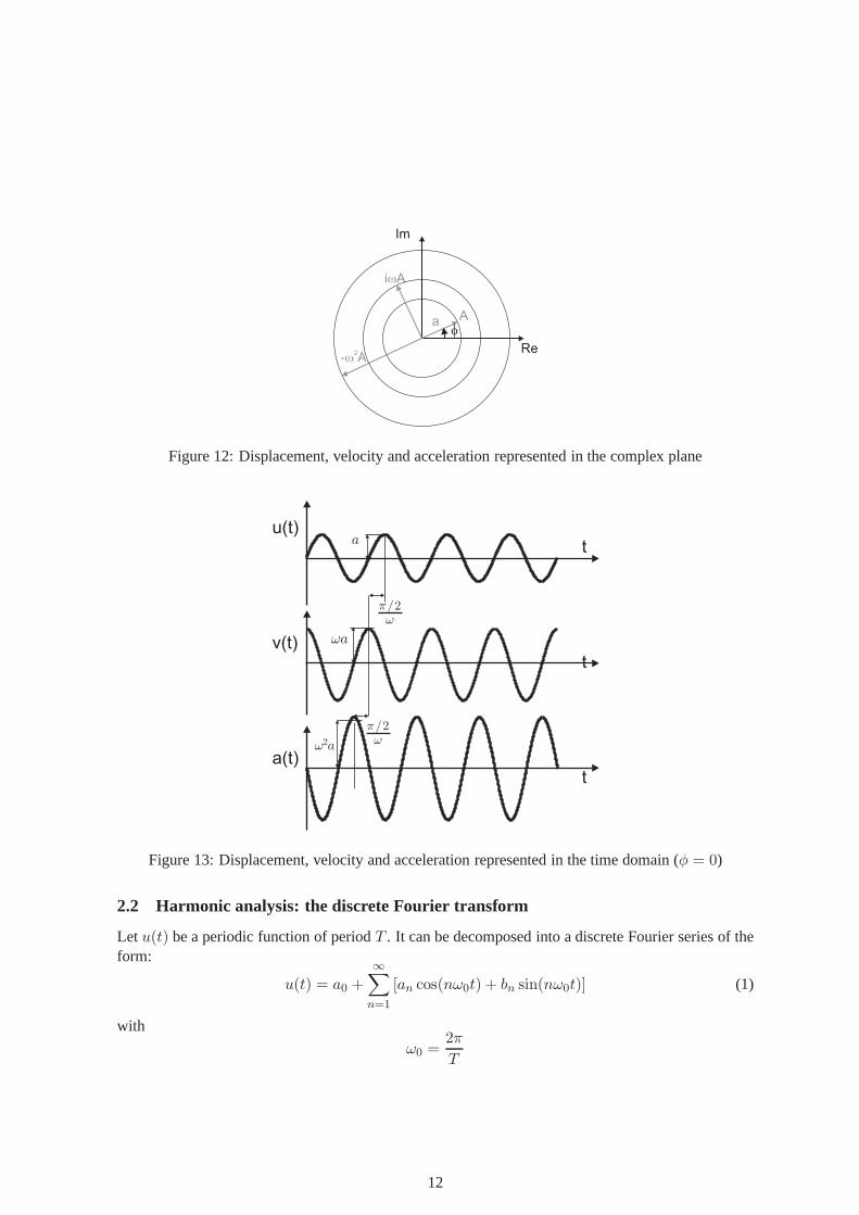
The displacement, velocity and accelerations are represented in the complex plane in Figure 12. Onecan see clearly that the derivation introduces a phase shiftof 90° together with a multiplication of theamplitude by a factorω. The signals are represented in the time domain for a phase angle ofφ = 0 inFigure 13.

11

Re

Im

f

i Aw

A

- Aw2

a

Figure 12: Displacement, velocity and acceleration represented in the complex plane

u(t)

v(t)

a(t)

!ù=2

!ù=2

!2a

!a

at

t

t

Figure 13: Displacement, velocity and acceleration represented in the time domain (φ = 0)

2.2 Harmonic analysis: the discrete Fourier transform

Let u(t) be a periodic function of periodT . It can be decomposed into a discrete Fourier series of theform:

u(t) = a0 +

∞∑

n=1

[an cos(nω0t) + bn sin(nω0t)] (1)

with

ω0 =2π

T

12

is the fundamental frequency and

a0 =1

T

∫ T

0u(t)dt (2)

an =2

T

∫ T

0u(t) cos(nω0t)dt (3)

bn =2

T

∫ T

0u(t) sin(nω0t)dt (4)

In other words, a peridic function can be represented by an infinite sum of sine and cosine functionsof discrete frequencies which are multiples of the fundamental frequencyω0 (Figure 14).

t

period T

f(t)

t

T

cos ( t)w0

t

T

cos (2 t)w0

t

T

sin ( )w0t

t

T

sin (2 t)w0

cos (n t)w0 sin (n t)w0

... ...Figure 14: Fourier decomposition of a periodic signal

13

An alternative formulation is given by:

u(t) =a02

+∞∑

n=1

[an cos(nω0t) + bn sin(nω0t)] (5)

a0 =2

T

∫ T

0u(t)dt

an =2

T

∫ T

0u(t) cos(nω0t)dt

bn =2

T

∫ T

0u(t) sin(nω0t)dt

2.2.1 Amplitude and phase formulation

Equation (5) can be written in the form of a single cosine function with amplitude an phase as follows:

u(t) = d0 +∞∑

n=1

dn cos(nω0t− φn) (6)

where one can show (left as a demonstration) that:

d0 =a02

dn =√

a2n + b2n

φn = tg−1

(

bnan

)

2.2.2 Complex formulation

Equation (5) can also be written in a complex form. Using the following trigonometric equalities,

cos(nω0t) =einω0t + e−inω0t

2

sin(nω0t) =einω0t − e−inω0t

2i

one gets:

u(t) =a02

+

∞∑

n=1

[

aneinω0t + e−inω0t

2+ bn

einω0t − e−inω0t

2i

]

u(t) =a02

+

∞∑

n=1

[

an − ibn2

einω0t +an + ibn

2e−inω0t

]

which can also be written

u(t) =

n=∞∑

n=−∞

cneinω0t

14

with

c0 =a02

cn =an − ibn

2

c−n =an + ibn

2

Subsitutinga0, an andbn using (2-4), we get:

c0 =a02

=1

T

∫ T

0u(t)dt

cn =an − ibn

2=

1

T

∫ T

0u(t) (cos(nω0t)− i sin(nω0t)) dt =

1

T

∫ T

0u(t)e−inω0tdt

c−n =an + ibn

2=

1

T

∫ T

0u(t) (cos(nω0t) + i sin(nω0t)) dt =

1

T

∫ T

0u(t)einω0tdt

so that we can finally write:

u(t) =

n=∞∑

n=−∞

cneinω0t (7)

with

c0 =1

T

∫ T

0u(t)dt

cn =1

T

∫ T

0u(t)e−inω0tdt

Note thatcn is complex and carries the phase and amplitude information of thenth component ofthe Fourier transform. This can easily be shown knowing that:

cn =an − ibn

2

dn =√

a2n + b2n

φn = tg−1

(

bnan

)

wheredn andφn are the phase and amplitudes of thenth component of the Fourier transform. Notealso thatcn andc−n are complex conjugate so thatu(t) is always real. The complex formulation canalso be written in the following form where the integrals aretaken from−T/2 to T/2 instead of from0 to T :

u(t) =

n=∞∑

n=−∞

cneinω0t

c0 =1

T

∫ T

2

−T

2

u(t)dt

cn =1

T

∫ T

2

−T

2

u(t)e−inω0tdt

15

2.2.3 Examples of Fourier transforms of periodic signals

d1 d2 d3 d4 d5 d6 d7 d8 d9 d10

1

T/2T/2

1

1

d10 d20 d30 d40 d50

Main frequencyband of signal

Time signalAmplitude of Fourier

coefficients

T/2T/2

T/2T/2

d1 d2 d3 d4 d5 d6 d7 d8 d9 d10

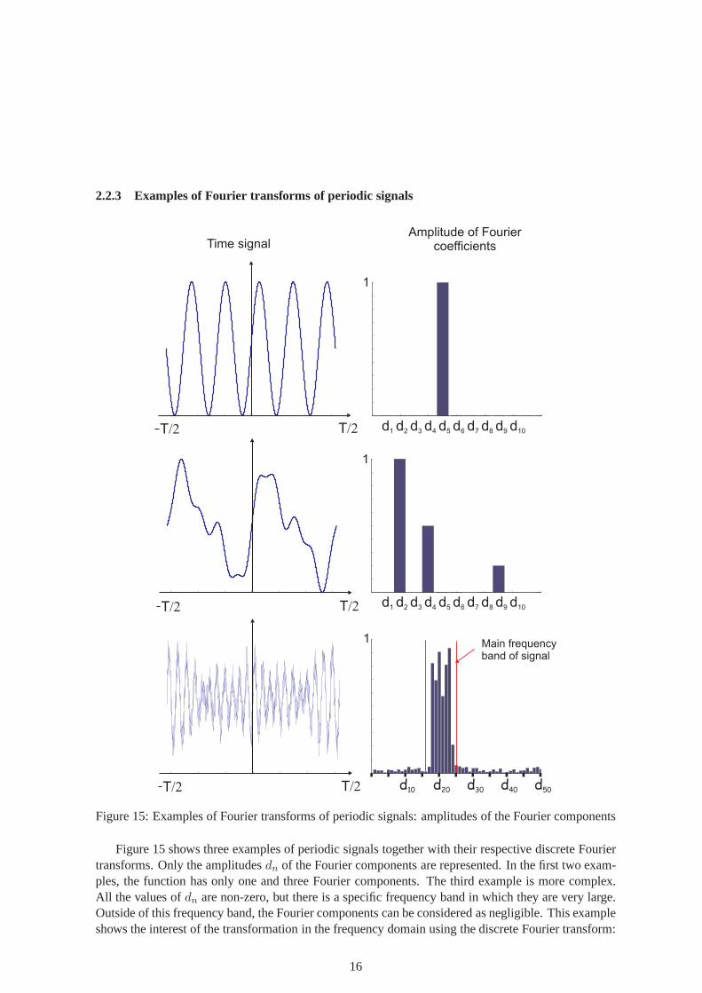
Figure 15: Examples of Fourier transforms of periodic signals: amplitudes of the Fourier components

Figure 15 shows three examples of periodic signals togetherwith their respective discrete Fouriertransforms. Only the amplitudesdn of the Fourier components are represented. In the first two exam-ples, the function has only one and three Fourier components. The third example is more complex.All the values ofdn are non-zero, but there is a specific frequency band in which they are very large.Outside of this frequency band, the Fourier components can be considered as negligible. This exampleshows the interest of the transformation in the frequency domain using the discrete Fourier transform:

16

if one wishes to compute the response of a structure to an excitation signal of that type, it should beperformed only in the main frequency band where the excitation signal has large Fourier components.

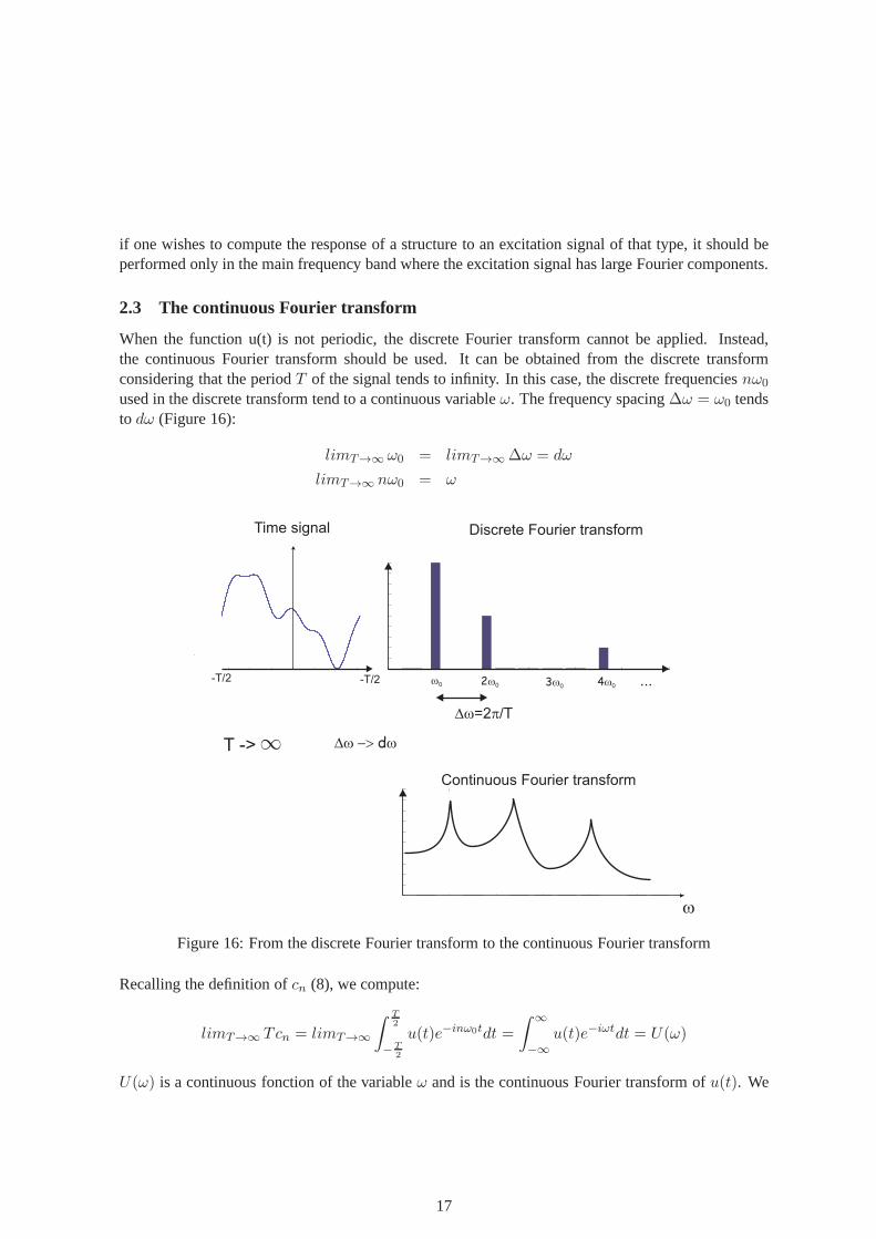
2.3 The continuous Fourier transform

When the function u(t) is not periodic, the discrete Fouriertransform cannot be applied. Instead,the continuous Fourier transform should be used. It can be obtained from the discrete transformconsidering that the periodT of the signal tends to infinity. In this case, the discrete frequenciesnω0

used in the discrete transform tend to a continuous variableω. The frequency spacing∆ω = ω0 tendsto dω (Figure 16):

limT→∞ ω0 = limT→∞∆ω = dω

limT→∞ nω0 = ω

-T/2 -T/2 w0 2w0 3w0 4w0 ...

Dw p=2 /T

Time signal Discrete Fourier transform

Continuous Fourier transform

w

1T -> Dw -> wd

Figure 16: From the discrete Fourier transform to the continuous Fourier transform

Recalling the definition ofcn (8), we compute:

limT→∞ Tcn = limT→∞

∫ T

2

−T

2

u(t)e−inω0tdt =

∫ ∞

−∞u(t)e−iωtdt = U(ω)

U(ω) is a continuous fonction of the variableω and is the continuous Fourier transform ofu(t). We

17

can now rewriteu(t):

u(t) = limT→∞

n=∞∑

n=−∞

cneinω0t = limT→∞

n=∞∑

n=−∞

cnT

Teinω0t

= limT→∞

n=∞∑

n=−∞

(cnT )ω0

2πeinω0t =

1

2π

∫ ∞

−∞U(ω)eiωtdω

which is the inverse continuous Fourier transform. Note that an alternative formulation consists inwriting the Fourier transform as a function off instead ofω. In this case, we have:

ω = 2πf ⇒ dω = 2πdf

U(f) =

∫ ∞

−∞u(t)e−i2πftdt

u(t) =

∫ ∞

−∞U(f)ei2πftdf

where one sees that the factor1/2π is not present anymore.

2.3.1 Examples of continuous Fourier transforms and properties

Table 1 and Figure 17 give a few examples of continuous Fourier transforms, while Table 2 gives someproperties of the continuous Fourier transforms. These properties will be used in the demonstrationof Parseval’s theorem in section 2.4.

u(t) U(f)

1 δ(f)δ(t) 1

cos(2πf0t)δ(f − f0) + δ(f + f0)

2

sin(2πf0t)δ(f − f0) + δ(f + f0)

2in=∞∑

n=−∞

δ(t− nT )1

T

n=∞∑

n=−∞

δ(f − n

T)

Table 1: Examples of continuous Fourier transforms

18

Time domain function Frequency domain function Property

a f(t) + b g(t) aF (f) + bG(f) Linearity

f(kt)1

|k|F(

f

k

)

Time Scaling

1

kf

(

t

k

)

F (kf) Frequency scaling

f(t− t0) e−i2πft0F (f) Time shiftingf(t) ei2πf0t F (f − f0) Frequency shifting

f(t) real even function F (f) real even functionf(t) real odd function F (f) imag odd function

f(t) real F (−f) = F (f)∗

Table 2: Properties of the continuous Fourier transform

t w

w

w

w

t

t

t

f(t) F( )w

F( )w

F( )w

F( )w

f(t)

f(t)

f(t)

1

1

T 1/T

f0-f0

1/f0

Figure 17: Examples of continuous Fourier transforms

In the following, we calculate the continuous Fourier transform of a cosine function, of a ’box’

19

function and a triangular function. Consider the functionu(t) = cos(2πf0t). Its Fourier transform isgiven by:

U(f) =

∫ ∞

−∞cos(2πf0t)e

−i2πft dt

=

∫ ∞

−∞

1

2

(

ei2πf0t + e−i2πf0t)

e−i2πft dt

=1

2

∫ ∞

−∞e−i2π(f−f0)t dt+

1

2

∫ ∞

−∞e−i2π(f+f0)t dt

=1

2δ(f − f0) +

1

2δ(f + f0)

where we have used the definition of theδ(x) function :

δ(x) =

∫ ∞

−∞e−2iπkx dk

Consider now the box function represented in Figure 18 whichis defined using the Heaviside stepfunctionH(x):

- 1 0 0 1 0

- 0 .4

- 0 .2

0

0 .2

0 .4

0 .6

0 .8

1

t

H(t+a)-H(t-a)

a-a

2a

1

Figure 18: Box function of width2a

u(t) = H(t+ a)−H(t− a) =

1 −a < t < 00 |t| > a

The continuous Fourier transform is:

U(f) =

∫ ∞

−∞u(t)e−i2πft dt =

∫ a

−ae−i2πft dt =

−1

i2πf

[

e−i2πft]a

−a

=(ei2πfa − e−i2πfa)

2iπf=

2 sin(2πfa)

2πf

Using the definition of thesinc function:

sinc(x) =sin(πx)

πx

we getU(f) = 2asinc(2fa)

20

Thesinc function is represented on Figure 19.

- 1 0 - 5 0 5 1 0

- 0 .4

- 0 .2

0

0 .2

0 .4

0 .6

0 .8

1

f

sinc(f) 11

Figure 19: Thesinc function

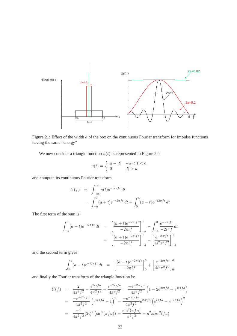
The effect of the widtha of the box is illustrated on Figure 20: as the width is dividedby a factorof 5, the value ofU(0) is divided by 5 (U(0) corresponds to the integral ofu(t), here the area of thebox), and the first lobe of thesinc function goes to zero for a value of 5 instead of 1. In order to seethe effect of the width of the box for functions having the same ”energy”, we consider now three boxfunctions of different widths, where the surface of the box is equal in Figure 21. The term ”energy”is used here to refer to the case whereu(t) is an impulse input force of duration∆t and amplitudeF , of which the energy isF∆t. For the same energy, we see that as the width of the box is smallerand smaller (i.e. the impact of the force is of shorter duration), the first lobe of thesinc function iswider and wider so that the continuous Fourier transform tends to a constant in the frequency bandconsidered in the graph. This illustrates the fact that in order to excite a wide band of frequencies withhigh amplitudes, the duration of the impact force must be as short as possible.

- 1 0 0 1 0

- 0 .4

- 0 .2

0

0 .2

0 .4

0 .6

0 .8

1

t

u(t)=H(t+a)-H(t-a)

0.5-0.5

2a=1

2a=0.2

1

- 5 0 5

- 0 .2

- 0 .1

0

0 .1

0 .2

0 .3

0 .4

0 .5

2a=1

2a=0.2

f

U(f)

1 5

Figure 20: Effect of the widtha of the box on the continuous Fourier transform

21

- 1 0 0 1 00

1

2

3

4

5

t

H(t+a)-H(t-a)

0.5-0.5

2a=1

2a=0.2

- 5 0 5

- 0 .2

- 0 .1

0

0 .1

0 .2

0 .3

0 .4

0 .5

2a=1

2a=0.2

2a=0.02

f

U(f)

1 5

Figure 21: Effect of the widtha of the box on the continuous Fourier transform for impulse functionshaving the same ”energy”

We now consider a triangle functionu(t) as represented in Figure 22:

u(t) =

a− |t| −a < t < a0 |t| > a

and compute its continuous Fourier transform

U(f) =

∫ ∞

−∞u(t)e−i2πft dt

=

∫ 0

−a(a+ t)e−i2πft dt+

∫ a

0(a− t)e−i2πft dt

The first term of the sum is:

∫ 0

−a(a+ t)e−i2πft dt =

[

(a+ t)e−2πift

−2πif

]0

−a

−∫ 0

−a

e−2πift

−2iπfdt

=

[

(a+ t)e−2πift

−2πif

]0

−a

−[

e−2iπft

4i2π2f2

]0

−a

and the second term gives

∫ a

0(a− t)e−i2πft dt =

[

(a− t)e−2πift

−2πif

]a

0

+

[

e−2iπft

4i2π2f2

]a

0

and finally the Fourier transform of the triangle function is:

U(f) =2

4π2f2− e2iπfa

4π2f2− e−2iπfa

4π2f2=

−e−2iπfa

4π2f2

(

1− 2e2iπfa + e4iπfa)

=−e−2iπfa

4π2f2

(

e2iπfa − 1)2

=−e−2iπfa

4π2f2e2iπfa

(

eiπfa − e−iπfa)2

=−1

4π2f2(2i)2

(

sin2(πfa))

=sin2(πfa)

π2f2= a2sinc2(fa)

22

00

t

u(t)

a-a

2a

a

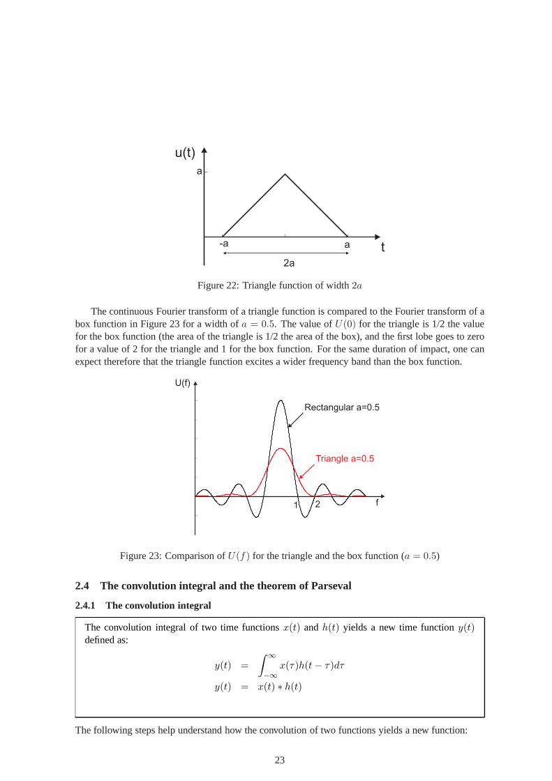
Figure 22: Triangle function of width2a

The continuous Fourier transform of a triangle function is compared to the Fourier transform of abox function in Figure 23 for a width ofa = 0.5. The value ofU(0) for the triangle is 1/2 the valuefor the box function (the area of the triangle is 1/2 the area of the box), and the first lobe goes to zerofor a value of 2 for the triangle and 1 for the box function. Forthe same duration of impact, one canexpect therefore that the triangle function excites a widerfrequency band than the box function.

- 0 .2

- 0 .1

0

0 .1

0 .2

0 .3

0 .4

0 .5

Rectangular a=0.5

Triangle a=0.5

f

U(f)

1 2

Figure 23: Comparison ofU(f) for the triangle and the box function (a = 0.5)

2.4 The convolution integral and the theorem of Parseval

2.4.1 The convolution integral

The convolution integral of two time functionsx(t) andh(t) yields a new time functiony(t)defined as:

y(t) =

∫ ∞

−∞x(τ)h(t− τ)dτ

y(t) = x(t) ∗ h(t)

The following steps help understand how the convolution of two functions yields a new function:

23

• Take the two functionsx(t) andh(t) and replace t by the dummy variableτ

• Mirror the functionh(τ) against the ordinate, this yieldsh(−τ)

• Shift the functionh(−τ) with a quantityt

• Determine for each value oft the product ofx(τ) with h(t− τ)

• Compute the integral of the producty(t)

• Let t vary from−∞ (or a value small enough to make the product zero) to+∞ (or a value oftthat is big enough)

Let us illustrate these different steps with an example. We consider the box functionx(t) which hasa unit value fromt = 0 to t = 1, and the box functionh(t) which has a value of 1/2 fromt = 0 tot = 1 (Figure 24).

1

1/2

1

x(t)

1 1t t

h(t)

Figure 24: Box functionsx(t) andh(t)

We replace variablet by τ and mirror theh(τ) function (Figure 25).

1

1/2

1

x( )tx( )t h(- )t

1 -1t t

Figure 25:x(τ) andh(−τ)

We then shift the functionh(−τ) with a quantityt (Figure 26).

1/2

h(t- )t

tt

Figure 26: h(t− τ)

24

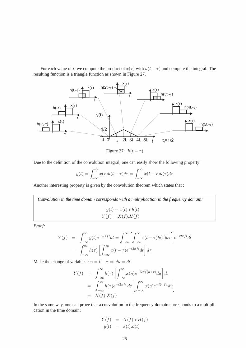
For each value oft, we compute the product ofx(τ) with h(t− τ) and compute the integral. Theresulting function is a triangle function as shown in Figure27.

y(t)

tt1 2t1 3t1 4t1 5t1-t1 0

1/2

x( )t

t

h(-t - )1 t

x( )t

t

h(- )t

x( )t

t

h(t - )1 t

x( )t

t

h(2t - )1 tx( )t

h(3t - )1 t

x( )th(4t - )1 t

x( )th(5t - )1 t

t =1/21

Figure 27: h(t− τ)

Due to the definition of the convolution integral, one can easily show the following property:

y(t) =

∫ ∞

−∞x(τ)h(t − τ)dτ =

∫ ∞

−∞x(t− τ)h(τ)dτ

Another interesting property is given by the convolution theorem which states that :

Convolution in the time domain corresponds with a multiplication in the frequency domain:

y(t) = x(t) ∗ h(t)Y (f) = X(f).H(f)

Proof:

Y (f) =

∫ ∞

−∞y(t)e−i2πftdt =

∫ ∞

−∞

[∫ ∞

−∞x(t− τ)h(τ)dτ

]

e−i2πftdt

=

∫ ∞

−∞h(τ)

[∫ ∞

−∞x(t− τ)e−i2πftdt

]

dτ

Make the change of variables :u = t− τ ⇒ du = dt

Y (f) =

∫ ∞

−∞h(τ)

[∫ ∞

−∞x(u)e−i2πf(u+τ)du

]

dτ

=

∫ ∞

−∞h(τ)e−i2πfτdτ

[∫ ∞

−∞x(u)e−i2πfudu

]

= H(f).X(f)

In the same way, one can prove that a convolution in the frequency domain corresponds to a multipli-cation in the time domain:

Y (f) = X(f) ∗H(f)

y(t) = x(t).h(t)

25

2.4.2 The theorem of Parseval

The energy of a signal computed in the time domain is equal to the energy computed in thefrequency domain :

∫ ∞

−∞h2(t)dt =

∫ ∞

−∞|H(f)|2df

Proof:

∫ ∞

−∞h2(t)dt =

∫ ∞

−∞

[∫ ∞

−∞H(f)ei2πftdf

] [∫ ∞

−∞H(f ′)ei2πf

′tdf ′]

dt

=

∫ ∞

−∞

∫ ∞

−∞H(f).H(f ′)

∫ ∞

−∞ei2π(f+f ′)tdtdf ′df

=

∫ ∞

−∞

∫ ∞

−∞H(f).H(f ′)

∫ ∞

−∞1 ei2π(f+2f ′)te−i2π(f ′)tdtdf ′df

The term∫ ∞

−∞1 ei2π(f+2f ′)te−i2π(f ′)tdt

is the Fourier transform of1 ei2π(f+2f ′)t = f(t) ei2π(f+2f ′)t

if we takef(t)=1. Knowing that the Fourier transform off(t)e2iπf0t is equal toF (f − f0) (seeTable 2), and that the Fourier transform of1 is δ(f) (Table 1), we have

∫ ∞

−∞1 ei2π(f+2f ′)te−i2π(f ′)tdt = δ(f ′ − (f + 2f ′)) = δ(−f − f ′)

and∫ ∞

−∞h2(t)dt =

∫ ∞

−∞

∫ ∞

−∞H(f).H(f ′)δ(−f − f ′)df ′df =

∫ ∞

−∞H(f).H(−f)df

In addition, we know that h(t) is real so that we have (Table 2)

H(−f) = H∗(f)

and finally

=

∫ ∞

−∞H(f).H∗(f)df =

∫ ∞

−∞|H(f)|2df

The theorem of Parseval can also be written using the variableω = 2πf :∫ ∞

−∞h2(t)dt =

∫ ∞

−∞|H(f)|2df =

1

2π

∫ ∞

−∞|H(ω)|2dω

26

3 Single degree of freedom system

The study of the single degree of freedom (dof) system is the foundation of structural dynamics. Sucha system is represented by a mass attached to the ground with aspring. One may argue that sucha system is not of practical importance, as buildings are nota large mass attached to the ground bya spring. While this is true, we will see in the next chapters that the theory of the single degree offreedom system can be used to study the dynamic behavior of all structures, once the concept of modeshapes is understood (Section 5.1). There are also cases forwhich the structure can be simplified tothe extent that it corresponds to a single dof system. This isthe subject of the next section.

3.1 One degree of freedom systems in real life

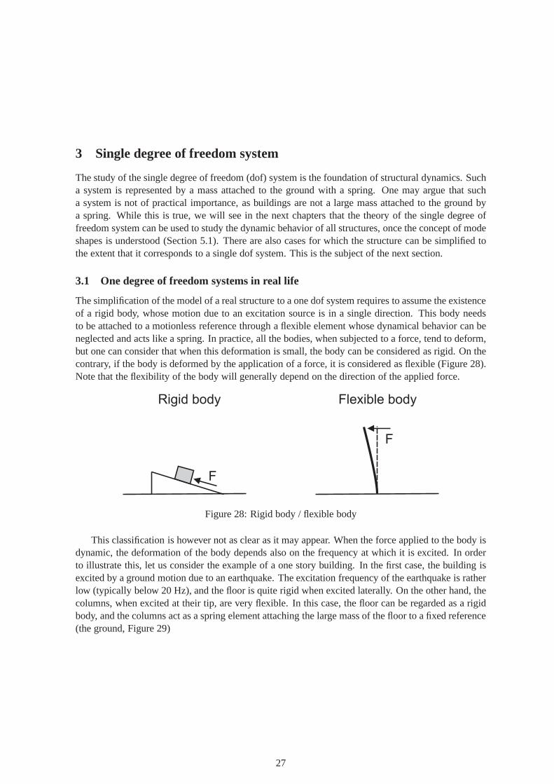
The simplification of the model of a real structure to a one dofsystem requires to assume the existenceof a rigid body, whose motion due to an excitation source is ina single direction. This body needsto be attached to a motionless reference through a flexible element whose dynamical behavior can beneglected and acts like a spring. In practice, all the bodies, when subjected to a force, tend to deform,but one can consider that when this deformation is small, thebody can be considered as rigid. On thecontrary, if the body is deformed by the application of a force, it is considered as flexible (Figure 28).Note that the flexibility of the body will generally depend onthe direction of the applied force.

F

Rigid body

F

Flexible body

Figure 28: Rigid body / flexible body

This classification is however not as clear as it may appear. When the force applied to the body isdynamic, the deformation of the body depends also on the frequency at which it is excited. In orderto illustrate this, let us consider the example of a one storybuilding. In the first case, the building isexcited by a ground motion due to an earthquake. The excitation frequency of the earthquake is ratherlow (typically below 20 Hz), and the floor is quite rigid when excited laterally. On the other hand, thecolumns, when excited at their tip, are very flexible. In thiscase, the floor can be regarded as a rigidbody, and the columns act as a spring element attaching the large mass of the floor to a fixed reference(the ground, Figure 29)

27

Ground motion

Rigid floor

Flexible columns km

Ground motion

Flexible columns

Rigid floor

Figure 29: One story Building excited by an earthquake

In the second case, if the building is excited by a rotating machine (such as a power generator)which is in the middle of the floor (Figure 30) , the frequency of excitation is much higher and canreach several hundreds of Hertz. The excitation of the rotating machine acts both in the vertical andin the horizontal direction. The horizontal direction corresponds to the case previously studied. Forthe vertical direction however, the columns have a much higher stiffness in that direction, and can beconsidered as rigid supports of the floor which is now excitedin bending, a direction in which it ismuch more flexible. The system can therefore be modeled by a beam on its supports which is excitedin the middle by a vertical force. In such a case, it is not straightforward to simplify the system to aone dof system (we will see however in section 6 how this can bedone).

Flexible floor

Rigid columns

Rotating machine

Rotating machine

Rigid columnsFlexible floor

Figure 30: One story building excited by a rotating machine

The first example shows how a real-life system can, in some cases, be simplified to a one dofsystem. In the second example, such a simplification is not asstraightforward. Note also that elementswhich are considered flexible in the first case, are considered rigid in the second case, and vice versa,the only difference being the direction of the excitation.

28

Figure 31 represents a series of systems which can be modeledwith an equivalent one dof system.

Ground motion

Rigid floor

Flexible columns km

Ground motion

Flexible columns

Rigid floor

Flexible mounts

Rigid stator

k

m

Flexible mounts

Rigid stator + rotor

Rigid rotor(unbalanced)

mr

Rigid rotor(unbalanced)

k

mFlexible suspensions

Rigid car

Flexible suspensions

Rigid car

Rigid wheelsRoad irregularities

Roadirregularities

km

f(t)

Rigid structure

Flexible foundations

Rigid structure

Flexible foundations

Waves excitation

k

m

Disk

Enginevibrations

Shaft

Disk

Shaft

Figure 31: Examples of equivalent one dof systems

29

3.2 Response of a single degree of freedom system without damping

Let us consider a mass-spring system without damping, represented in Figure 32. The first law ofNewton applied to this system gives:

mx =∑

Fx (8)

where∑

Fx is the sum of forces action on massm in directionx:

• Spring force: −kx , wherek is the stiffness of the spring. Note that the positionx = 0corresponds to the static equilibrium of the hanging mass attached to the spring. As the equationof motion is written with respect to this reference position, the force of gravity must not beconsidered in the equilibrium of forces: it is in equilibrium with the spring forcek∆l in thestatic equilibrium position (Fiugre 33)

• External forcef acting on the mass. It is the force which causes the mass to move, it is calledthe ”excitation force”.

Putting all the terms dependent onx on the left hand side, we get the equation of motion of the 1 dofsystem:

mx+ kx = f (9)

k

m

f

m

f

x

kx

x=0

Figure 32: Forces acting on a one dof mass-spring system

k

m mx=0

l0 l + l0 D

mg

k lD

Figure 33: Definition of the reference positionx = 0 of the mass for the mass-spring system

30

3.2.1 General solution of the equation of motion

The characteristics equation of (9) is obtained assumingx = Aert which leads to:

mr2 + k = 0 (10)

The roots of this equation are purely imaginary:

r = ±i√

k/m

The general solution can therefore be written in the form of :

x = A cos ωnt+B sinωnt

whereωn =

√

k/m

is the natural angular frequency. In the absence of externalexcitation force, the motion is oscillatorywith a frequencyf = 1

2π

√

k/m which is defined by the values of k and m.The motion is initializedby imposing initial conditions on the displacementx0 and on the velocityx0. In this case, the motionis given by:

x(t) = x0 cosωnt+x0ωn

sinωnt

Figure 34 illustrates the vibration of a one dof system to which an initial displacementx0 with a zeroinitial velocity x0 are imposed.

k

mxx0

x0

t

Figure 34: Free vibration of a 1 dof system to which an initialdisplacementx0 is imposed

The solution can also be written in the general form of a cosine with amplitudea and a phaseφ:

x(t) = a cos (ωnt+ φ)

where we have:

x0 = a cosφ

x0/ωn = a sinφ

which leads to:

tan φ =x0ωnx0

The phaseφ is a function of bothx0 andx0. It is equal to zero whenx0 = 0 and equal to90 whenx0 = 0.

31

3.2.2 Particular solution

Consider the continuous inverse Fourier transform of the excitation forcef(t):

f(t) =1

2π

∫ ∞

−∞F (ω)e−iωtdω

and isolate a single component at frequencyω:

F (ω)e−iωt = F (ω) cos(ωt) + iF (ω) sin(ωt)

Let us first consider an excitation of the formF (ω) cos(ωt). The equilibrium equation is written:

mx+ kx = F cosωt (11)

and the particular solution can be written in the general form

x(t) = A cos ωt+B sinωt = a cos(ωt+ φ)

If we now consider an excitation of the formF (ω) sin(ωt), the form of the general solution is

x(t) = a sin(ωt+ φ)

Therefore the general solution to an excitationF (ω)eiωt is

x(t) = a cos(ωt+ φ) + i sin(ωt+ φ) = aei(ωt+φ) = Xeiωt

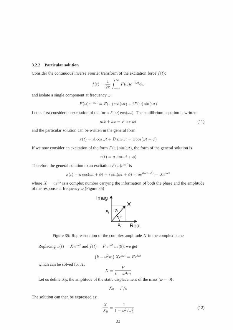
whereX = aeiφ is a complex number carrying the information of both the phase and the amplitudeof the response at frequencyω (Figure 35)

af

xr

xi

Real

Imag

X

Figure 35: Representation of the complex amplitudeX in the complex plane

Replacingx(t) = X eiωt andf(t) = F eiωt in (9), we get

(

k − ω2m)

Xeiωt = Feiωt

which can be solved forX:

X =F

k − ω2m

Let us defineX0, the amplitude of the static displacement of the mass (ω = 0) :

X0 = F/k

The solution can then be expressed as:

X

X0=

1

1− ω2/ω2n

(12)

32

where we have used the fact thatωn =√

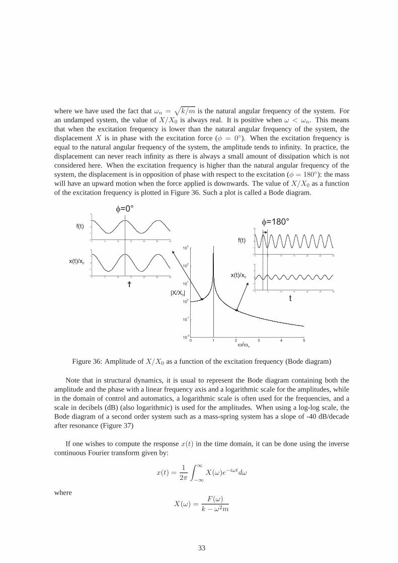
k/m is the natural angular frequency of the system. Foran undamped system, the value ofX/X0 is always real. It is positive whenω < ωn. This meansthat when the excitation frequency is lower than the naturalangular frequency of the system, thedisplacementX is in phase with the excitation force (φ = 0). When the excitation frequency isequal to the natural angular frequency of the system, the amplitude tends to infinity. In practice, thedisplacement can never reach infinity as there is always a small amount of dissipation which is notconsidered here. When the excitation frequency is higher than the natural angular frequency of thesystem, the displacement is in opposition of phase with respect to the excitation (φ = 180): the masswill have an upward motion when the force applied is downwards. The value ofX/X0 as a functionof the excitation frequency is plotted in Figure 36. Such a plot is called a Bode diagram.

0 1 2 3 4 510

-2

10-1

100

101

102

103

w w/ n

|X/X |0

0 5 10 15 20 25 30-2

-1

0

1

2

0 5 10 15 20 25 30-2

-1

0

1

2

0 5 10 15 20 25 30-2

-1

0

1

2

0 5 10 15 20 25 30-2

-1

0

1

2

f=180°

f=0°

t

x(t)/x0

f(t)

t

x(t)/x0

f(t)

Figure 36: Amplitude ofX/X0 as a function of the excitation frequency (Bode diagram)

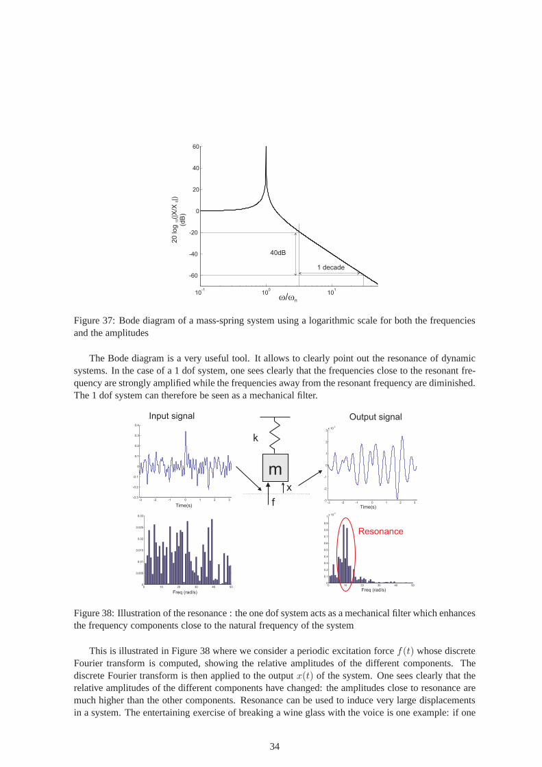
Note that in structural dynamics, it is usual to represent the Bode diagram containing both theamplitude and the phase with a linear frequency axis and a logarithmic scale for the amplitudes, whilein the domain of control and automatics, a logarithmic scaleis often used for the frequencies, and ascale in decibels (dB) (also logarithmic) is used for the amplitudes. When using a log-log scale, theBode diagram of a second order system such as a mass-spring system has a slope of -40 dB/decadeafter resonance (Figure 37)

If one wishes to compute the responsex(t) in the time domain, it can be done using the inversecontinuous Fourier transform given by:

x(t) =1

2π

∫ ∞

−∞X(ω)e−iωtdω

where

X(ω) =F (ω)

k − ω2m

33

10-1

100

101

-60

-40

-20

0

20

40

60

w w/ n

20 log

(|X

/X|)

(dB

)1

00

40dB

1 decade

Figure 37: Bode diagram of a mass-spring system using a logarithmic scale for both the frequenciesand the amplitudes

The Bode diagram is a very useful tool. It allows to clearly point out the resonance of dynamicsystems. In the case of a 1 dof system, one sees clearly that the frequencies close to the resonant fre-quency are strongly amplified while the frequencies away from the resonant frequency are diminished.The 1 dof system can therefore be seen as a mechanical filter.

-3 -2 -1 0 1 2 3-0.3

-0.2

-0.1

0

0.1

0.2

0.3

0.4

Time(s)

0 10 20 30 40 500

0.005

0.01

0.015

0.02

0.025

0.03

Freq (rad/s)

-3 -2 -1 0 1 2 3-3

-2

-1

0

1

2

3x 10

-3

Time(s)

0 10 20 30 40 500

0.1

0.2

0.3

0.4

0.5

0.6

0.7

0.8

0.9

1x 10

-3

k

m

f

x

Freq (rad/s)

Resonance

Input signal Output signal

Figure 38: Illustration of the resonance : the one dof systemacts as a mechanical filter which enhancesthe frequency components close to the natural frequency of the system

This is illustrated in Figure 38 where we consider a periodicexcitation forcef(t) whose discreteFourier transform is computed, showing the relative amplitudes of the different components. Thediscrete Fourier transform is then applied to the outputx(t) of the system. One sees clearly that therelative amplitudes of the different components have changed: the amplitudes close to resonance aremuch higher than the other components. Resonance can be usedto induce very large displacementsin a system. The entertaining exercise of breaking a wine glass with the voice is one example: if one

34

emits a sounds whose frequency is close to one of the natural frequencies of the glass, the effect canbe strong enough to break it. The reader can see a demonstration in the following videos:

http://www.youtube.com/watch?v=10lWpHyN0Okhttp://www.youtube.com/watch?v=JiM6AtNLXX4

3.3 Response of a single degree of freedom system with damping

Equation (9) represents a conservative system in which there is an exchange between the kinetic andpotential energy without dissipation of energy. In reality, there is always a certain amount of energydissipated somewhere in the system, which is responsible for a certain amount of damping. For mass-spring systems, the most common form of damping adopted is the viscous damping, represented bya dashpot element. In the equation of motion, an additional force due to the dashpot is added in thefollowing form:

Fb = −bxThe equation of motion is given by (Figure 39) :

mx+ bx+ kx = f (13)

In order to simplify the notations, equation (13) can be rewritten by dividing it bym and introducingthe damping coefficientξ = b/(2

√km):

x+ 2ξωnx+ ω2nx = f/m (14)

k

m

f

m

f

x

kx

x=0

bbx

Figure 39: Forces acting on a one dof mass-spring-dashpot system

3.3.1 General solution of the equation of motion

The characteristics equation is given by:

r2 + 2ξωnr + ω2n = 0

In most structures, the damping coefficientξ is smaller than one. In this case, the roots of the charac-teristics equations are given by:

r = −ξωn ± iωn

√

1− ξ2

orr = −ξωn ± iωd

35

withwd = ωn

√

1− ξ2

The general solution can be written in the form of:

x(t) = e−ξωnt (A cosωdt+B sinωdt)

In the absence of external forces, the system will vibrate due to initial conditions on the displacementx0 and the velocityx0. The free vibration is given by:

x(t) = e−ξωnt

(

x0 cosωdt+x0 + ωnξx0

ωdsinωdt

)

(15)

The system will oscillate at a frequencyωd which is different from the natural frequencyωn, and themotion will decrease with time due to the exponential terme−ξωnt which is a function of the dampingcoefficientξ and the natural frequency of the systemωn. The free response is represented for differentvalues ofξ in Figure 40.

0 20 40 60 80 100 120 140-1

-0.8

-0.6

-0.4

-0.2

0

0.2

0.4

0.6

0.8

1

0 20 40 60 80 100 120 140-1

-0.8

-0.6

-0.4

-0.2

0

0.2

0.4

0.6

0.8

1

0 20 40 60 80 100 120 140-1

-0.8

-0.6

-0.4

-0.2

0

0.2

0.4

0.6

0.8

1

0 20 40 60 80 100 120 140-0.8

-0.6

-0.4

-0.2

0

0.2

0.4

0.6

0.8

1

x=0 x=0.01

x=0.05 x=0.1

t

x x

xx

t

tt

Figure 40: Free vibration of a one dof mass-spring-dashpot system due to an initial unit displacementx0 = 1 as a function of the damping coefficientξ

When ξ = 0, the mass oscillates with a constant amplitude. As the damping increases, theamplitude decreases faster with time. For a value ofξ = 0.01, the amplitude is divided by 2 afterabout 10 oscillations. On Figure 41, we represent the numbern of oscillations needed to decreasethe amplitude by one half as a function ofξ, in a log-log scale. The figure shows clearly that as thedamping coefficient is divided by 10, 10 times more oscillations are needed to reduce the amplitude byone half. The time needed for the motion of the mass to be reduced by one half is a function ofξ andthe natural frequencyωn: the higherωn, the shorter this time will be. For a system with a low naturalfrequency and a low level of damping, a very long time will be needed to attenuate the vibration.

36

10-3

10-2

10-1

100

101

102

x

n

Figure 41: Numbern of oscillations needed to reduce the vibration amplitude byone half as a functionof the damping coefficientξ

When the damping coefficient is very high (ξ > 1), the solution of the equation of motion is:

x(t) = e−ξωnt

(

x0 cosh µt+x0 + ωnξx0

µsinhµt

)

withµ = ωn

√

ξ2 − 1

This solution is not oscillatory. The higher the damping, the slower the response decreases because ofthecosh andsinh terms which grow with time. For a limit value ofξ = ∞, the mass is blocked by thedamper in the initial position (x(t) = x0, Figure 42). The valueξ = 1 represents the limit betweenthe oscillatory motion and the non-oscillatory motion. This value is called the critical damping. Theroots of the characteristics equation are double and given by:

r = −ωn

The solution is given by:x(t) = e−ωnt ((x0 + ωnx0) t+ x0)

It is represented on Figure 42. Note that the critical damping corresponds to the value of damping forwhich the motion of the mass is the fastest to reach a zero value.

0 2 4 6 8 10

-0.8

-0.6

-0.4

-0.2

0

0.2

0.4

0.6

0.8

1

x=0.1

x=1

x=2

x=100

x(t)

t (s)

Figure 42: Response of a one dof mass-spring-dashpot systemto an initial unit displacement (x0 = 1)for high values of damping coefficientsξ

37

3.3.2 The impulse response

An impulse excitation is defined as a force of amplitudeF applied during a short time∆t. The energyof the impulse is given byF∆t (Figure 43). Let us consider the equation of motion (13) withinitialconditionsx0 = 0 andx0 = 0 and integrate it fromt = 0 to t = ∆t:

mx0|∆t = F∆t−∫ ∆t

0kxdt−

∫ ∆t

0bxdt

As the initial conditions arex0 = 0 and x0 = 0 and the time interval∆t is very short, the last twoterms tend to zero, we get:

x0|∆t =F∆t

m

which shows that in order to compute the response of a system to an impulseF∆t, one has to computethe response to an imposed velocityF∆t/m at timet = ∆t. The impulse response of the system isdefined as the response to a unit value ofF∆t. Using (15), the impulse response is given by:

x(t) =e−ξωnt

mωdsin(ωdt) (16)

F

tDt

Impulse=F tD

Figure 43: Definition of an impulse excitation

3.3.3 Particular solution of the equation of motion

In a similar way to what was done for the undamped system, we assumef(t) = Feiωt andx(t) =Xeiωt and replace in (14) to get:

(ω2n + 2iξωωn − ω2)X = F/m

The complex amplitudeX is given by:

X =F

m

(

1

ω2n + 2iξωωn − ω2

)

=F

k

(

1

1− ω2

ω2n

+ 2iξ ωωn

)

= X0

(

1

1− ω2

ω2n

+ 2iξ ωωn

)

The real and imaginary parts ofX are given by:

38

Xr = X0

1− ω2

ω2n

(

1− ω2

ω2n

)2+(

2ξ ωωn

)2

Xi = X0

−2ξ ωωn

(

1− ω2

ω2n

)2+(

2ξ ωωn

)2

and the amplitude and phase ofX/X0 are given by:

|X/X0| =

√

√

√

√

1(

1− ω2

ω2n

)2+(

2ξ ωωn

)2

tan φ =−2ξ ω

ωn

1− ω2

ω2n

The Bode diagram (amplitude and phase) ofX/X0 is represented in Figure 44 for different values ofξ.

0 0.5 1 1.5 2 2.5 3 3.5 4 4.5 510

-2

10-1

100

101

102

0 0.5 1 1.5 2 2.5 3 3.5 4 4.5 5-200

-150

-100

-50

0

w w/ n

|X/X |0

f(°)

x=0.01

x=0.1

x=0.3

x=1

x=0.01

x=1

x=0.3x=0.1

1à 2ø2p

Figure 44: Bode diagram for the one dof mass-spring-dashpotsystem. Influence of the dampingcoefficientξ

The influence ofξ is as follows: asξ is increased, the amplitude of the peak is reduced and thephase transition from0 to 180 around the resonance is smoother. At the resonant frequency, thephase is always equal to90. The frequency at which the amplitude is maximum is slightlydifferentfrom ωn andωd:

ω/ωn =√

1− 2ξ2

39

The maximum amplitude is given by

|X/X0| =1

2ξ√

1− ξ2

For small values ofξ, we have however:

ω/ωn = 1

|X/X0| =1

2ξ

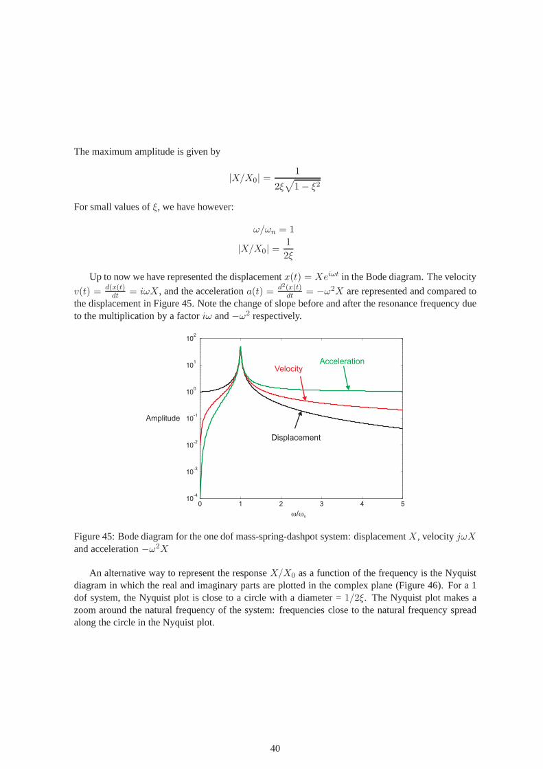
Up to now we have represented the displacementx(t) = Xeiωt in the Bode diagram. The velocity

v(t) = d(x(t)dt = iωX, and the accelerationa(t) = d2(x(t)

dt = −ω2X are represented and compared tothe displacement in Figure 45. Note the change of slope before and after the resonance frequency dueto the multiplication by a factoriω and−ω2 respectively.

0 1 2 3 4 510

-4

10-3

10-2

10-1

100

101

102

w w/ n

Amplitude

Displacement

VelocityAcceleration

Figure 45: Bode diagram for the one dof mass-spring-dashpotsystem: displacementX, velocityjωXand acceleration−ω2X

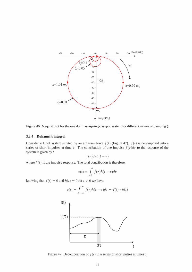
An alternative way to represent the responseX/X0 as a function of the frequency is the Nyquistdiagram in which the real and imaginary parts are plotted in the complex plane (Figure 46). For a 1dof system, the Nyquist plot is close to a circle with a diameter = 1/2ξ. The Nyquist plot makes azoom around the natural frequency of the system: frequencies close to the natural frequency spreadalong the circle in the Nyquist plot.

40

-30 -20 -10 0 10 20 30

-50

-45

-40

-35

-30

-25

-20

-15

-10

-5

x=0.01

x=0.05

x=0.1

w=0.99 wnw=1.01 wn

wn

w

Real(X/X )0

Imag(X/X )0

1/2x

1

Figure 46: Nyquist plot for the one dof mass-spring-dashpotsystem for different values of dampingξ

3.3.4 Duhamel’s integral

Consider a 1 dof system excited by an arbitrary forcef(t) (Figure 47). f(t) is decomposed into aseries of short impulses at timeτ . The contribution of one impulsef(τ)dτ to the response of thesystem is given by :

f(τ)dτh(t− τ)

whereh(t) is the impulse response. The total contribution is therefore:

x(t) =

∫ t

0f(τ)h(t− τ)dτ

knowing thatf(t) = 0 andh(t) = 0 for t > 0 we have:

x(t) =

∫ ∞

−∞f(τ)h(t− τ)dτ = f(t) ∗ h(t)

t

f(t)

dt

t

f( )t

Figure 47: Decomposition off(t) in a series of short pulses at timesτ

41

In the particular case wheref(t) = Feiωt, we have:

x(t) = Xeiωt =

∫ ∞

−∞Feiωth(t− τ)dτ =

∫ ∞

−∞Feiω(t−τ)h(τ)dτ

= Feiωt∫ ∞

−∞h(τ)e−iωτdτ = FeiωtH(ω)

which can be rewritten:

H(ω) =X

F

showing that the continuous Fourier transform of the impulse responseh(t) is the ratioX/F which isthe transfer function of the one dof system.

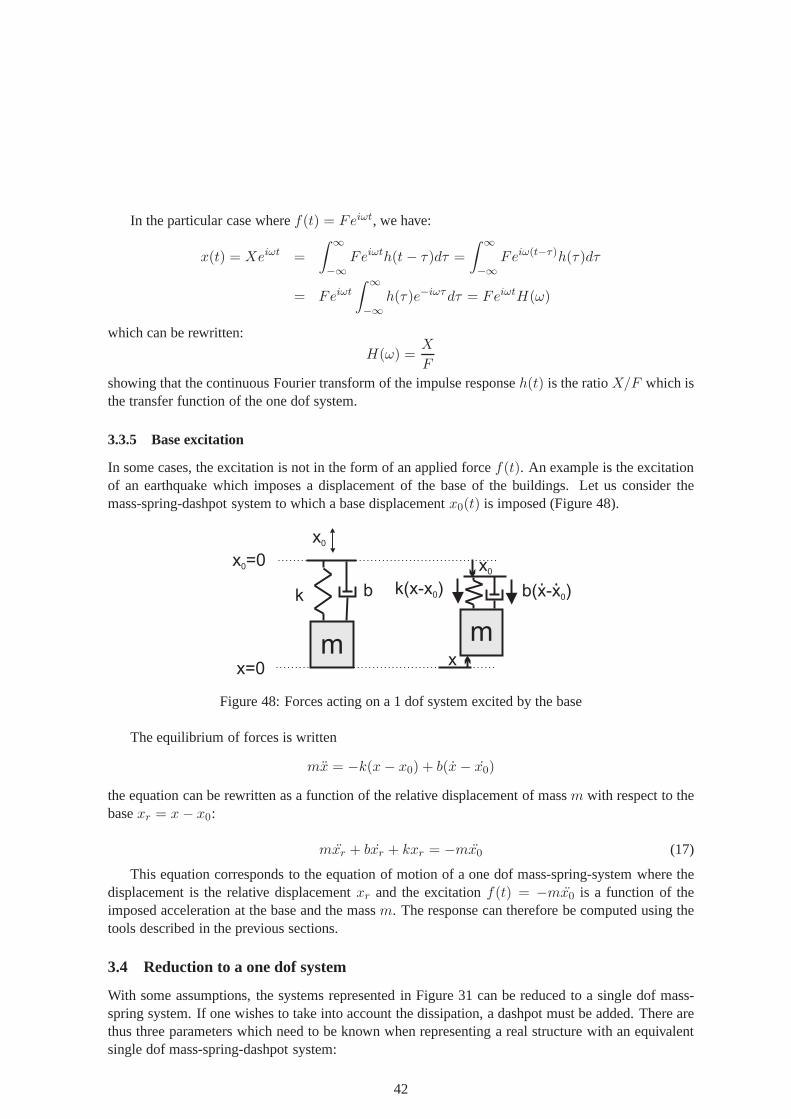
3.3.5 Base excitation

In some cases, the excitation is not in the form of an applied forcef(t). An example is the excitationof an earthquake which imposes a displacement of the base of the buildings. Let us consider themass-spring-dashpot system to which a base displacementx0(t) is imposed (Figure 48).

k

m m

x0

k(x-x )0

x=0

b

x0

x

b(x-x )0

x =00

Figure 48: Forces acting on a 1 dof system excited by the base

The equilibrium of forces is written

mx = −k(x− x0) + b(x− x0)

the equation can be rewritten as a function of the relative displacement of massm with respect to thebasexr = x− x0:

mxr + bxr + kxr = −mx0 (17)

This equation corresponds to the equation of motion of a one dof mass-spring-system where thedisplacement is the relative displacementxr and the excitationf(t) = −mx0 is a function of theimposed acceleration at the base and the massm. The response can therefore be computed using thetools described in the previous sections.

3.4 Reduction to a one dof system

With some assumptions, the systems represented in Figure 31can be reduced to a single dof mass-spring system. If one wishes to take into account the dissipation, a dashpot must be added. There arethus three parameters which need to be known when representing a real structure with an equivalentsingle dof mass-spring-dashpot system:

42

• The equivalent stiffnessk

• The equivalent massm

• The equivalent viscous damping coefficientb

One should always keep in mind that the equivalent single dofsystem is a simplification of the reality,and that it is valid only in a certain frequency range. This will be discussed in more details in sec-tion 3.4.4. With the help of simple examples, we illustrate the methodology to compute the equivalentstiffness, mass and damping parameters of a system.

3.4.1 Equivalent stiffness

The most general method to compute the equivalent stiffnessof the flexible element of the systemconsists in applying a force of amplitudeF in the direction of motion, and computing the resultingdisplacementx in the same direction. The equivalent stiffness is given byk = F/x (Figure 49).

m m

Flexiblebody

S

x

F

k=F/x

Directionof motion S

Figure 49: Principle to compute the equivalent stiffnessk of a flexible bodyS

In the following, this methodology is applied to simple flexible bodies, for which analytical solu-tions can be computed.

Bar in tractionFor a bar in traction (Figure 50), the constitutive equationis given by:

N = EAdu

dx

whereE is the Young’s modulus, A the area of the section andu(x) the axial displacement (in direc-tion x). For a bar in pure traction, the normal forceN is constant and equal toF so that the generalform of u(x) is

u(x) =F

EAx+ Cst

The bar is fixed (u(x)=0) atx = 0, so that we have :

u(x) =F

EAx

The displacement at the free tip of the bar is equal to

d =F

EAL

43

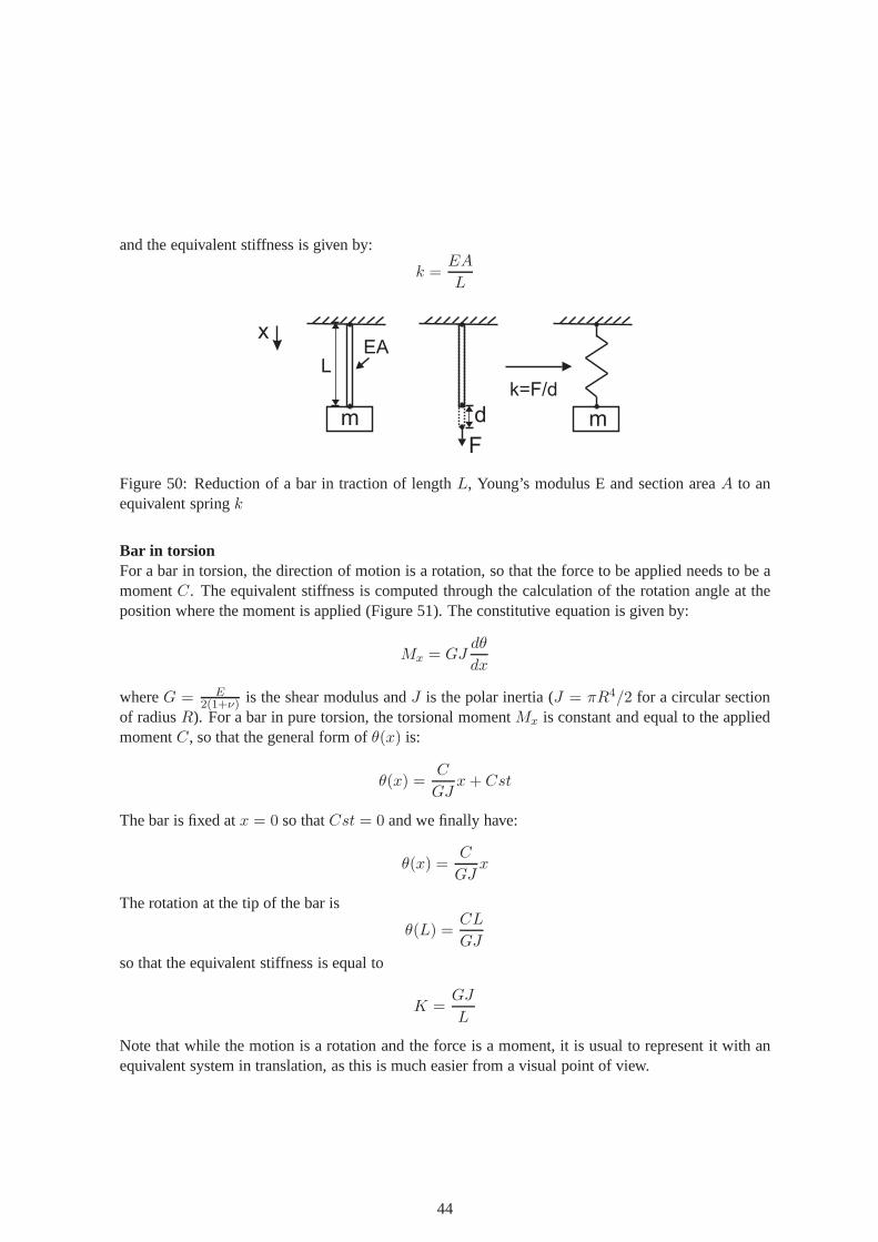
and the equivalent stiffness is given by:

k =EA

L

m m

EA

d

F

k=F/d

L

x

Figure 50: Reduction of a bar in traction of lengthL, Young’s modulus E and section areaA to anequivalent springk

Bar in torsionFor a bar in torsion, the direction of motion is a rotation, sothat the force to be applied needs to be amomentC. The equivalent stiffness is computed through the calculation of the rotation angle at theposition where the moment is applied (Figure 51). The constitutive equation is given by:

Mx = GJdθ

dx

whereG = E2(1+ν) is the shear modulus andJ is the polar inertia (J = πR4/2 for a circular section

of radiusR). For a bar in pure torsion, the torsional momentMx is constant and equal to the appliedmomentC, so that the general form ofθ(x) is:

θ(x) =C

GJx+ Cst

The bar is fixed atx = 0 so thatCst = 0 and we finally have:

θ(x) =C

GJx

The rotation at the tip of the bar is

θ(L) =CL

GJ

so that the equivalent stiffness is equal to

K =GJ

L

Note that while the motion is a rotation and the force is a moment, it is usual to represent it with anequivalent system in translation, as this is much easier from a visual point of view.

44

I

GJ

C

K=C/Q

L

x

QC

I

Figure 51: Reduction of a bar in torsion of lengthL and torsional stiffnessGJ to an equivalent springK

Beam in bendingFor beams in bending, we can follow the same approach as the one detailed for the bar in traction andin torsion. In most cases however, it is more convenient to use solutions directly available in tables. Asan example, we consider a cantilever beam in bending (Figure52). From the tables, we can directlyget the displacementy(x) as a function ofx:

y(x) =Fx2

6EI(3L− x)

and deduce the tip displacement

y(L) = d =FL3

3EI

The equivalent stifness is therfore

k =3EI

L3

m

mEI

d F

k=F/dL

xk

Figure 52: Reduction of a beam in bending of lengthL and bending stiffnessEI to an equivalentspringk

Let us take a second example of a portal frame represented in Figure 53. The direction of motionis supposed to be horizontal. Due to the symmetry of the structure, the problem can be studied byconsidering only one half of the structure. The force applied in the direction of motion is thusF/2.Note that the boundary conditions of the beam in bending are different from the previous example,because the rotation at the tip is zero due to fixation to the rigid floor. For these boundary conditions,the displacement is given by:

y(x) =F

24EIx2(3L− 2x)

The tip displacement is

d = y(L) =FL3

24EI

45

which gives us the value of the equivalent stiffness

k =24EI

L3

If we neglect the weight of the columns, the natural frequency of the equivalent one dof system is

f =1

2π

√

24EI

L3Mfloor(Hz)

Mfloor

FF/2

EIEI, r

d

d

Figure 53: Reduction of a portal frame to an equivalent mass-spring system

An alternative method can be used to compute the equivalent stiffness. It is based on the equalityof the strain energy of the real structure and the one dof mass-spring system which is given by

Es =kx2

2=F 2

2k(18)

The principle consists in computing the strain energy of thereal system and then identifying theequivalent stiffness by expressing the equality with (18).Let us consider the first three examples:

• For a bar in traction, the strain energy is

Es =1

2

∫ L

0

N2

EAdx

and the normal forceN is constant and equal toF leading to

Es =1

2

F 2L

EA=F 2

2k⇒ k =

EA

L

• For a bar in torsion, the strain energy is

Es =1

2

∫ L

0

M2x

GJdx

and the torsional momentMx is constant and equal toC leading to

Es =1

2

C2L

GJ=C2

2K⇒ K =

GJ

L

46

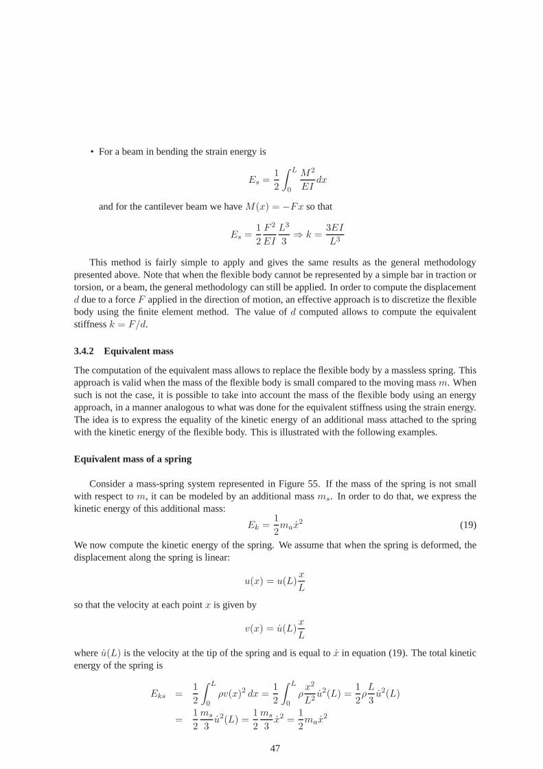
• For a beam in bending the strain energy is

Es =1

2

∫ L

0

M2

EIdx

and for the cantilever beam we haveM(x) = −Fx so that

Es =1

2

F 2

EI

L3

3⇒ k =

3EI

L3

This method is fairly simple to apply and gives the same results as the general methodologypresented above. Note that when the flexible body cannot be represented by a simple bar in traction ortorsion, or a beam, the general methodology can still be applied. In order to compute the displacementd due to a forceF applied in the direction of motion, an effective approach isto discretize the flexiblebody using the finite element method. The value ofd computed allows to compute the equivalentstiffnessk = F/d.

3.4.2 Equivalent mass

The computation of the equivalent mass allows to replace theflexible body by a massless spring. Thisapproach is valid when the mass of the flexible body is small compared to the moving massm. Whensuch is not the case, it is possible to take into account the mass of the flexible body using an energyapproach, in a manner analogous to what was done for the equivalent stiffness using the strain energy.The idea is to express the equality of the kinetic energy of anadditional mass attached to the springwith the kinetic energy of the flexible body. This is illustrated with the following examples.

Equivalent mass of a spring

Consider a mass-spring system represented in Figure 55. If the mass of the spring is not smallwith respect tom, it can be modeled by an additional massms. In order to do that, we express thekinetic energy of this additional mass:

Ek =1

2max

2 (19)

We now compute the kinetic energy of the spring. We assume that when the spring is deformed, thedisplacement along the spring is linear:

u(x) = u(L)x

L

so that the velocity at each pointx is given by

v(x) = u(L)x

L

whereu(L) is the velocity at the tip of the spring and is equal tox in equation (19). The total kineticenergy of the spring is

Eks =1

2

∫ L

0ρv(x)2 dx =

1

2

∫ L

0ρx2

L2u2(L) =

1

2ρL

3u2(L)

=1

2

ms

3u2(L) =

1

2

ms

3x2 =

1

2max

2

47

wherems is the mass of the spring (ms = ρL). The additional mass due to the spring isma = ms/3.

m m

L

x

k,ms

ma

k

Figure 54: Equivalent 1D model of a mass-spring system taking into account the additional mass dueto the spring

Bar in tractionThe second example is a mass hanging from a bar. We have already calculated the equivalent stiffnessof the bar in tractionk = EA/L. When the mass of the bar is not small compared to the massm, itsequivalent additional massma needs to be computed. Again, we assume that the displacementis inthe form

u(x) = u(L)x

L

the velocity is

v(x) = u(L)x

L

whereu(L) is the velocity at the tip of the bar and is equal tox in equation (19). Following the samecalculations as for the spring, the additional massma is equal tomb/3 wheremb is the mass of thebar.

m

EA, r L

m

x

F

ma

EA, r L

x

F

d

k=EA/L

Figure 55: Equivalent mass-spring model of a mass hanging from a bar taking into account the addi-tional mass due to the bar

3.4.3 Equivalent damping

In real structures, damping is a complex phenomenon which comes mainly from two types of sources:external and internal (Figure 56).

48

Damping

Internal External

Material Connections(joints, bearings)

Non-structural elements,energy radition in soil

Figure 56: Sources of damping in real structures

When dissipation is present, the stress is not in phase with the strain, which results in a hysteresisloop if one plots the stress as a function of the strain (Figure 57).

0

t

û

"

û

"Epot

WD

Figure 57: When the stress is not in phase with the strain (left), this results in a hysteresis loop in thestress-strain plane (right)

The mechanical energy dissipated in one cycle per unit volumeWD is given by the area inside theloop :

WD =

∫ T

0σε dt =

∫

σdε

whereT is the period of one cycle. The damping factorψ of a material is proportional to the ratio ofenergy dissipated in one cycle to the maximum strain potential energy:

ψ =1

2π

WD

Epot

whereEpot is the maximum strain energy. The damping factor of a structure is given by

ψS =

∫

Vψ dV =

1

2π

WDS

EpotS

It is equal to the damping factor of the material if the structure is homogeneous. The methodology tocompute an equivalent viscous damping coefficient consistsin expressing the equality ofψS for thestructure studied, with the value ofψS for a one dof mass-spring-dashpot system.

49

Computation of ψS for a single dof mass-spring dashpot system

Let us consider the mass-spring-dashpot system represented in Figure 58 and compute the dissi-pated energy in one cycle:

WDS =

∫ T

0bx xdt

with x(t) = |X|cos(ωt) we have

WDS =

∫ T

0ω2b|X|2sin2(ωt)dt =

∫ T

0ω2b|X|2 1− cos(2ωt)

2dt

= ω2b|X|2T2

= πbω|X|2

k

m

f

x=0

b

Figure 58: One dof mass-spring-dasphot system

The maximum potential energy is given by

EpotS =1

2kx2max =

1

2k|X|2

and the damping factor of the mass-spring-dashpot system isgiven by:

ΨS =1

2π

WDS

EpotS=

2π

2π

bω|X|2k|X|2

=ωb

k

Note that the damping factor the mass-spring-dashpot system computed at the natural frequencyω =√

k/m is:

ψS(ωn) =

√

k

m

b

k=

b√km

= 2ξ

showing the link with the damping coefficientξ defined earlier.

Examples of computation of an equivalent damping

Let us consider a few examples of computation of an equivalent dampingb.

• In the general case whereψS is a known function ofω, we have:

b(ω) =kψS(ω)

ω

50

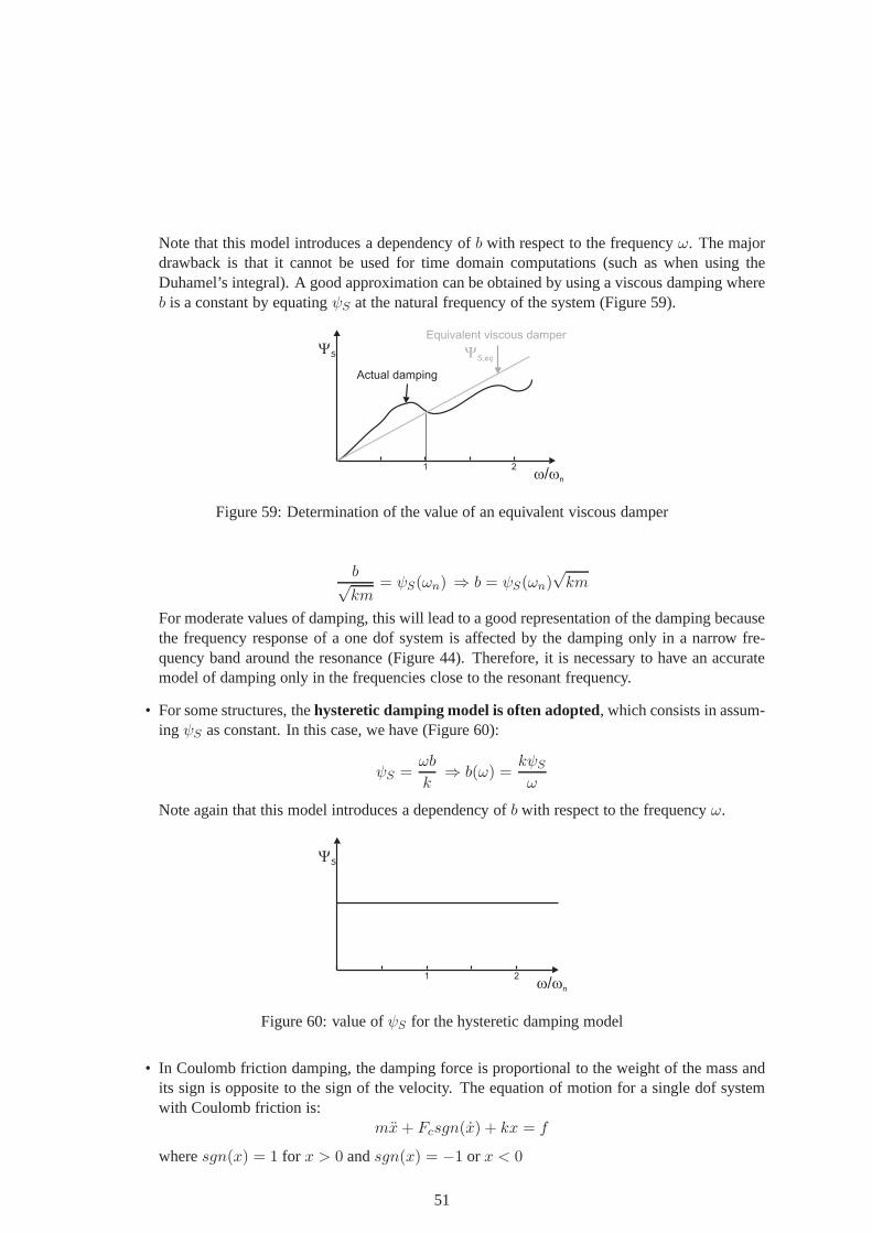
Note that this model introduces a dependency ofb with respect to the frequencyω. The majordrawback is that it cannot be used for time domain computations (such as when using theDuhamel’s integral). A good approximation can be obtained by using a viscous damping whereb is a constant by equatingψS at the natural frequency of the system (Figure 59).

Actual damping

Equivalent viscous damper

w w/ n

1 2

YS,eqYS

Figure 59: Determination of the value of an equivalent viscous damper

b√km

= ψS(ωn) ⇒ b = ψS(ωn)√km

For moderate values of damping, this will lead to a good representation of the damping becausethe frequency response of a one dof system is affected by the damping only in a narrow fre-quency band around the resonance (Figure 44). Therefore, itis necessary to have an accuratemodel of damping only in the frequencies close to the resonant frequency.

• For some structures, thehysteretic damping model is often adopted, which consists in assum-ing ψS as constant. In this case, we have (Figure 60):

ψS =ωb

k⇒ b(ω) =

kψS

ω

Note again that this model introduces a dependency ofb with respect to the frequencyω.

w w/ n

YS

1 2

Figure 60: value ofψS for the hysteretic damping model

• In Coulomb friction damping, the damping force is proportional to the weight of the mass andits sign is opposite to the sign of the velocity. The equationof motion for a single dof systemwith Coulomb friction is:

mx+ Fcsgn(x) + kx = f

wheresgn(x) = 1 for x > 0 andsgn(x) = −1 or x < 0

51

km

f(t)

Coulomb friction

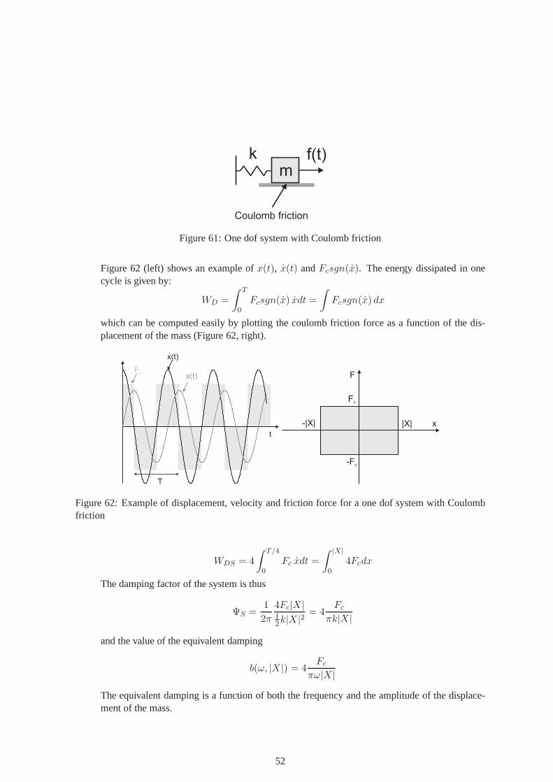
Figure 61: One dof system with Coulomb friction

Figure 62 (left) shows an example ofx(t), x(t) andFcsgn(x). The energy dissipated in onecycle is given by:

WD =

∫ T

0Fcsgn(x) xdt =

∫

Fcsgn(x) dx

which can be computed easily by plotting the coulomb friction force as a function of the dis-placement of the mass (Figure 62, right).

x(t).

x(t)

T

Fc

t

F

Fc

x|X|

-Fc

-|X|

Figure 62: Example of displacement, velocity and friction force for a one dof system with Coulombfriction

WDS = 4

∫ T/4

0Fc xdt =

∫ |X|

04Fcdx

The damping factor of the system is thus

ΨS =1

2π

4Fc|X|12k|X|2

= 4Fc

πk|X|

and the value of the equivalent damping

b(ω, |X|) = 4Fc

πω|X|

The equivalent damping is a function of both the frequency and the amplitude of the displace-ment of the mass.

52

Measurement of damping in one dof systems

Typical values of damping for materials used in civil engineering structures are given in Table 3.Because the damping in structures comes from the materials but also from the connections, it isvery difficult to predict the damping coefficient of a structure. Because of that, it is often necessaryto measure the damping coefficient after the structure has been built in order to make sure that thestructure is safe. There are two fast and simple techniques to measure this damping coefficient.

Material ξ

Reinforced concrete 0.004-0.012Composite 0.002-0.003Steel 0.001-0.002

Table 3: Typical values of damping in civil engineering structures

The first technique is called thelogarithmic decrement method. It is based on the measurementof the impulse response of the structure. When a structure isexcited by an impulse force, the responsecontains mainly its first mode. This is because the form of theimpulse response is a sine functionwith an exponentially decaying enveloppe where the coefficient of the exponential is−ξωnt. Thehigher modes decrease therefore faster and their contribution to the response is negligible after a fewoscillations. A typical impulse response containing only the first mode of vibration (single dof) isrepresented in Figure 63.

t

x(t)

xn

Xn+m

m periods

Figure 63: Impulse response containing the first mode (single dof)

The general form of the response at timet is:

x(t) = e−ξωnt (Acos(ωdt) +Bsin(ωdt))

The responsem periods after timet is:

x(t+mT ) = e−ξωn(t+mT ) (Acos(ωd(t+mT )) +Bsin(ωd(t+mT )))

x(t+mT ) = e−ξωn(t+mT ) (Acos(ωdt) +Bsin(ωdt))

and we havex(t)

x(t+mT )=

e−ξωnt

e−ξωn(t+mT )= eξωn(mT )

53

we define the logarithmic decrement

Λ = ln

(

x(t)

x(t+mT )

)

= ξωn(mT ) = ξm2π

ωdωn = 2mπξ

1√

1− ξ2

For small values ofξ we haveξ2 << 1 which gives:

Λ ≃ 2mπξ

The damping coefficient is given by:

ξ =1

2πmΛ

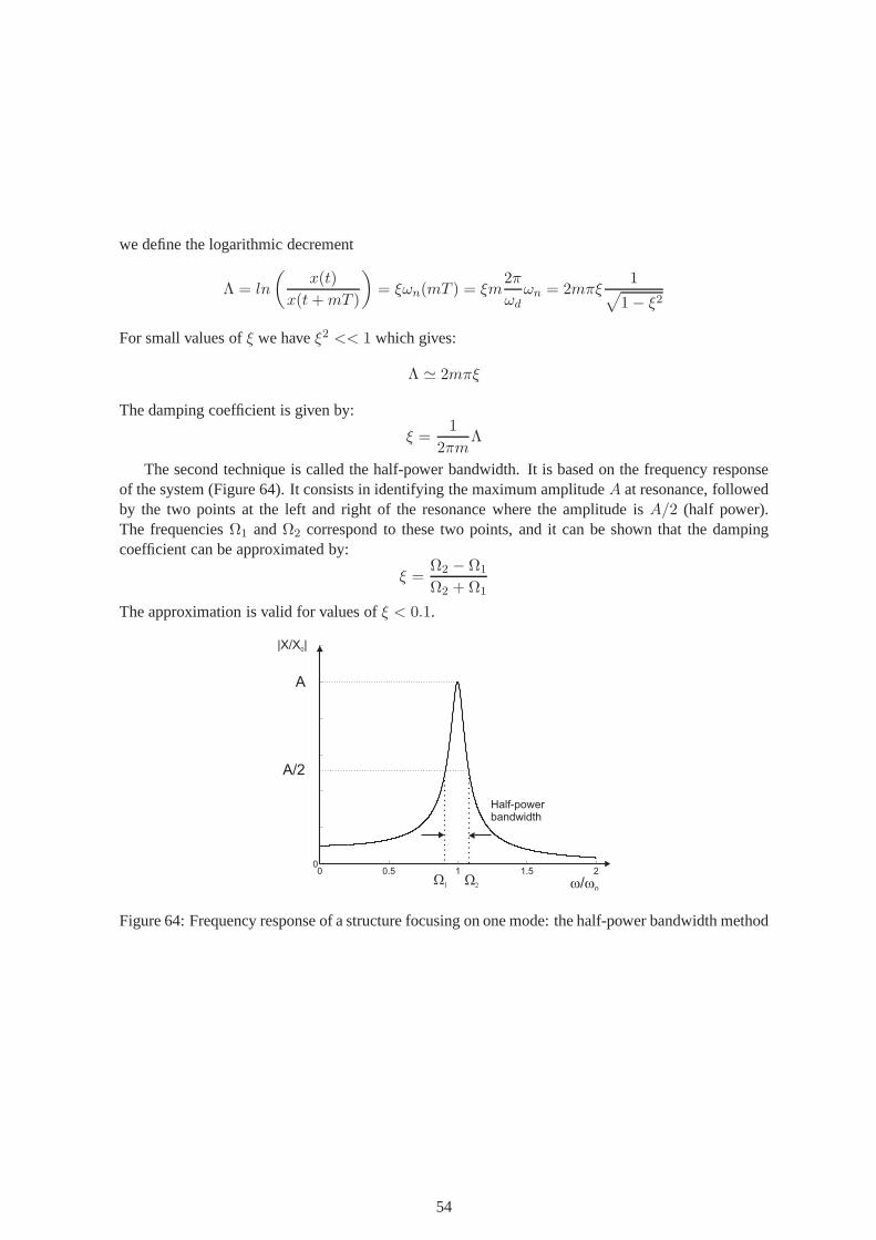
The second technique is called the half-power bandwidth. Itis based on the frequency responseof the system (Figure 64). It consists in identifying the maximum amplitudeA at resonance, followedby the two points at the left and right of the resonance where the amplitude isA/2 (half power).The frequenciesΩ1 andΩ2 correspond to these two points, and it can be shown that the dampingcoefficient can be approximated by:

ξ =Ω2 − Ω1

Ω2 +Ω1

The approximation is valid for values ofξ < 0.1.

0 0.5 1 1.5 20

w w/ n

|X/X |0

W1 W2

A

A/2

Half-powerbandwidth

Figure 64: Frequency response of a structure focusing on onemode: the half-power bandwidth method

54

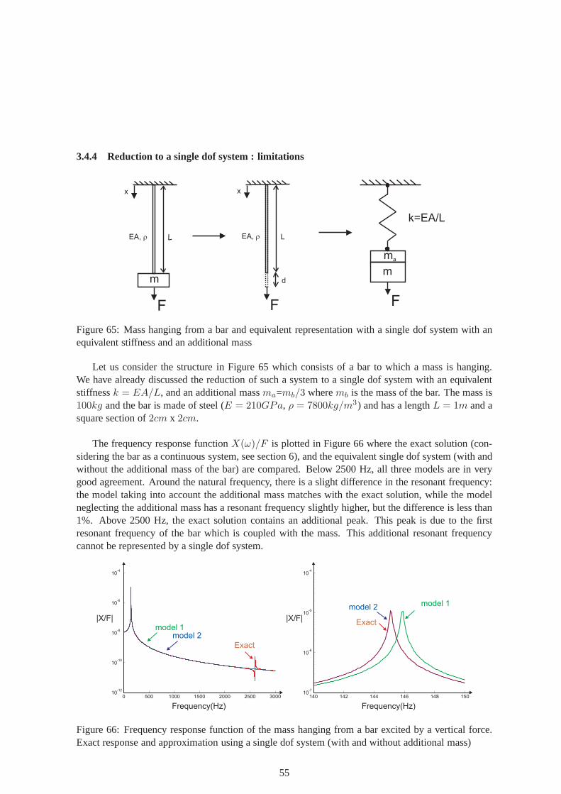
3.4.4 Reduction to a single dof system : limitations

m

EA, r L

x

F

EA, r L

x

F

d

k=EA/L

m

F

ma

Figure 65: Mass hanging from a bar and equivalent representation with a single dof system with anequivalent stiffness and an additional mass

Let us consider the structure in Figure 65 which consists of abar to which a mass is hanging.We have already discussed the reduction of such a system to a single dof system with an equivalentstiffnessk = EA/L, and an additional massma=mb/3 wheremb is the mass of the bar. The mass is100kg and the bar is made of steel (E = 210GPa, ρ = 7800kg/m3) and has a lengthL = 1m and asquare section of2cm x 2cm.

The frequency response functionX(ω)/F is plotted in Figure 66 where the exact solution (con-sidering the bar as a continuous system, see section 6), and the equivalent single dof system (with andwithout the additional mass of the bar) are compared. Below 2500 Hz, all three models are in verygood agreement. Around the natural frequency, there is a slight difference in the resonant frequency:the model taking into account the additional mass matches with the exact solution, while the modelneglecting the additional mass has a resonant frequency slightly higher, but the difference is less than1%. Above 2500 Hz, the exact solution contains an additionalpeak. This peak is due to the firstresonant frequency of the bar which is coupled with the mass.This additional resonant frequencycannot be represented by a single dof system.

0 500 1000 1500 2000 2500 300010

-12

10-10

10-8

10-6

10-4

Frequency(Hz)

Exact

model 1model 2

|X/F|

140 142 144 146 148 15010

-7

10-6

10-5

10-4

Frequency(Hz)

Exact

model 1model 2

|X/F|

Figure 66: Frequency response function of the mass hanging from a bar excited by a vertical force.Exact response and approximation using a single dof system (with and without additional mass)

55

The next graphs in Figure 67 are plotted using a value ofρ 10 times higher (i.e.ρ = 78000kg) forthe bar. While this value is not representative of a real material, the purpose is to illustrate the fact thatin such a case, the mass of the bar cannot be neglected anymore. We see indeed that if the mass of thebar is neglected, a significant difference is found for the first natural frequency. Another difference isthat the equivalent single dof model is only valid below 500 Hz due to the appearance of several peaksabove this value. These peaks are due to several resonant frequencies of the continuous bar coupledto the mass. Such additional peaks can again not be represented by a single dof system.

In summary, the examples shown above illustrate the fact that the single dof equivalent system isonly valid in a certain frequency band which depends on dynamic properties of the bodies which arereplaced by an equivalent mass and spring.

0 500 1000 1500 2000 2500 300010

-12

10-10

10-8

10-6

10-4

Frequency(Hz)

Exact

model 1

model 2

|X/F|

50 100 150 20010

-8

10-7

10-6

10-5

10-4

Frequency(Hz)

Exact

model 1model 2

|X/F|

Figure 67: Frequency response function of the mass hanging from a heavy bar excited by a verticalforce. Exact response and approximation using a single dof system (with and without additional mass)

3.5 One DOF application: the accelerometer

By far the most common sensor for measuring vibrations is theaccelerometer. The basic workingprinciple of such a device is presented in Figure 68(a). It consists of a moving mass on a spring anddashpot, attached to a moving solid. The acceleration of themoving solid results in a differentialdisplacementx between the massM and the solid. The governing equation is given by,

Mx+ cx+ kx = −Mx0 (20)

In the frequency domainx/x0 is given by,

x

x0=

−1

−ω2 + ω2n + 2iξωωn

(21)

with ωn =√

km andξ = b/2

√km and for frequenciesω << ωn, one has,

x

x0≃ −1

ω2n

(22)

showing that at low frequencies compared to the natural frequency of the mass-spring system,x isproportional to the accelerationx0. Note that since the proportionality factor is−1

ω2n

, the sensitivity

56

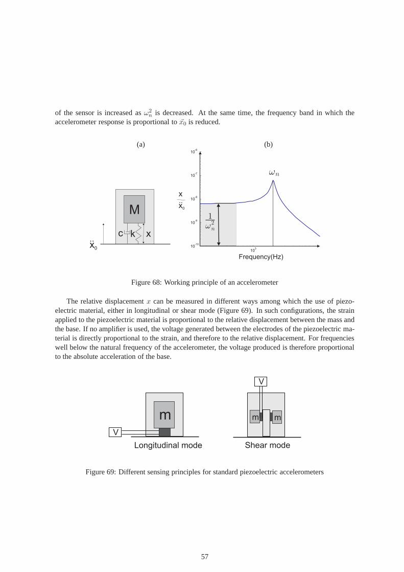
of the sensor is increased asω2n is decreased. At the same time, the frequency band in which the

accelerometer response is proportional tox0 is reduced.

(a) (b)

M

k xx0

..

103

10-10

10-9

10-8

10-7

10-6

Frequency(Hz)

!2

n

1

!n

x

x0

..

c

Figure 68: Working principle of an accelerometer

The relative displacementx can be measured in different ways among which the use of piezo-electric material, either in longitudinal or shear mode (Figure 69). In such configurations, the strainapplied to the piezoelectric material is proportional to the relative displacement between the mass andthe base. If no amplifier is used, the voltage generated between the electrodes of the piezoelectric ma-terial is directly proportional to the strain, and therefore to the relative displacement. For frequencieswell below the natural frequency of the accelerometer, the voltage produced is therefore proportionalto the absolute acceleration of the base.

m

Longitudinal mode

V

m

Shear mode

m

V

Figure 69: Different sensing principles for standard piezoelectric accelerometers

57

4 Vibration isolation

4.1 Direct vibration isolation

The problem of direct vibration isolation consists in preventing the vibrations coming from a givensource to propagate in the building, or in the surroundings.A typical example is the washing mashinewhich, when vibrating, transmits the vibration to the floor.Depending on the design of the building,such vibrations can propagate through several floors. Another example is a power station locatednear other buildings such as a school or a hotel. The vibrations generated by the power station canpropagate into the neighboring buildings and cause noise and discomfort. Schematically, the source ofvibrations is represented by a force f acting on a rigid body of massm. This rigid body is fixed to theground through some elements which are represented by a spring and a damper in parallel (Figure 70).

k

m

f

b

Figure 70: Direct vibration isolation

The equation of motion is:mx+ bx+ kx = f

The force transmitted to the ground (surroundings) is :

fT = bx+ kx

In the frequency domain, we have

F =(

k − ω2m+ iωb)

X ⇒ |F | =√

(k − ω2m)2 + ω2b2|X|

andFT = (k + iωb)X ⇒ |FT | =

√

k2 + ω2b2|X|The isolation factor is given by:

|FT ||F | =

√k2 + ω2b2

√

(k − ω2m)2 + ω2b2

and using the definitions ofξ = b/(2√km) andωn =

√

k/m we get :

|FT ||F | =

√

1 + (2ξ ωωn

)2

√

(1− ( ωωn

)2)2 + (2ξ ωωn

)2(23)

The isolation factor is a function of the frequencyω and is plotted in Figure 71.

58

0 1 2 3 4 510

-2

10-1

100

101

102

w w/ n

x=0.01

x=0.1

x=0.5

|F |/|F|<1T

Isolation domain

2p

Amplificationdomain

x=0.5

x=0.1

x=0.01

|F |/|F|T

Figure 71: Isolation factor for the direct vibration isolation problem

One can distinguish two different domains:

• for frequenciesω <√2ωn, |FT |/|F | > 1, this is the amplification domain where no isolation is

achieved, the amplitude of the force transmitted to the ground is greater than the force applied tothe body. In this domain, adding damping improves the situation: the amplification at resonancedecreases.

• for frequenciesω >√2ωn we are in the isolation domain: the force transmitted to the ground is

smaller than the forcef . In this domain, adding damping has a negative impact on the isolationwhich decreases.

For the damping, an ideal situation would be to have a damper which has a high damping at lowfrequencies and a low damping at high frequencies. Materials such as rubber and elastomers exhibitthat type of damping properties. The problem of direct vibration isolation consists in designing theone dof system such that for the excitation frequencies considered, we are in the isolation domain. Ifthese excitation frequencies are low, it requires to have a very low resonant frequency of the singledof system. There are two ways to achieve this: the first one isto have a very soft spring. Note thatthe spring must be strong enough to sustain the static load ofthe mass which in general does not allowto use very flexible springs. The second way is to increase themass of the system. This can be donefor example by adding a rigid and heavy foundation to the rigid body of massm.

4.2 Inverse vibration isolation

The problem of inverse vibration isolation consists in designing an isolator on which sensitive equip-ment is attached in order to prevent the vibrations from the environment to reach the sensitive equip-ment. Examples are precision devices such as microscopes orlithography machines which need to beisolated from ground motion, or buildings which need to be isolated from the ground motion due toearthquakes. Schematically, the vibrations from the environment are represented by a ground motionx, and the sensitive equipment is the rigid bodym attached to the ground through a spring and adamper (Figure 72).

59

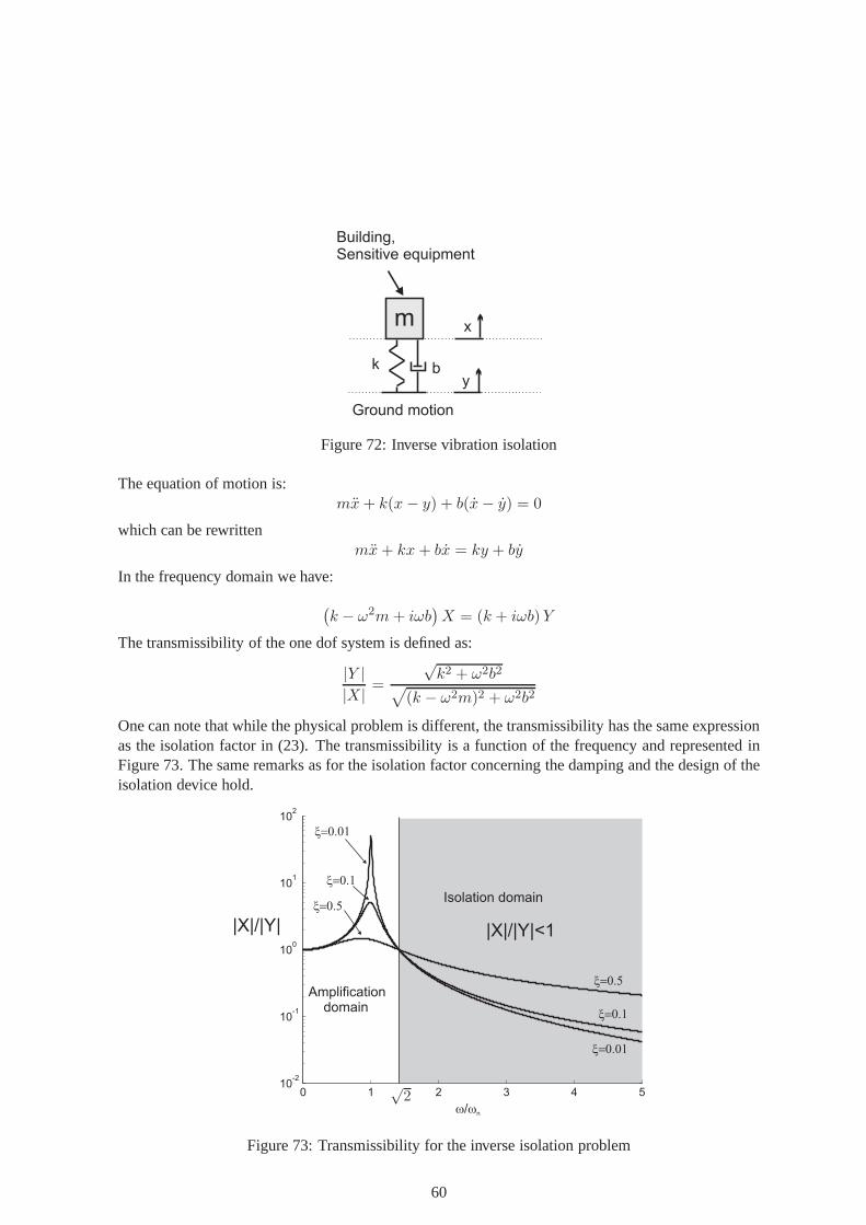
k

m

by

x

Ground motion

Building,Sensitive equipment

Figure 72: Inverse vibration isolation

The equation of motion is:mx+ k(x− y) + b(x− y) = 0

which can be rewrittenmx+ kx+ bx = ky + by

In the frequency domain we have:

(

k − ω2m+ iωb)

X = (k + iωb)Y

The transmissibility of the one dof system is defined as:

|Y ||X| =

√k2 + ω2b2

√

(k − ω2m)2 + ω2b2

One can note that while the physical problem is different, the transmissibility has the same expressionas the isolation factor in (23). The transmissibility is a function of the frequency and represented inFigure 73. The same remarks as for the isolation factor concerning the damping and the design of theisolation device hold.

0 1 2 3 4 510

-2

10-1

100

101

102

w w/ n

x=0.01

x=0.1

x=0.5

|X|/|Y|<1

Isolation domain

2p

Amplificationdomain

x=0.5

x=0.1

x=0.01

|X|/|Y|

Figure 73: Transmissibility for the inverse isolation problem

60

The following movies illustrate the effect of an isolator for different problems such as buildingisolation for earthquakes:

Vibration isolation demonstrations :http://www.youtube.com/watch?v=ntV6LQF1GxAhttp://www.youtube.com/watch?v=reYtUNLXvt8http://www.youtube.com/watch?v=YPAOZXc33gEhttp://www.youtube.com/watch?v=MboMuAzRUF0http://www.youtube.com/watch?v=ChaqMDc4ceshttp://www.youtube.com/watch?v=ZqlXp3czrrMhttp://www.youtube.com/watch?v=Fw7aQwMmBNM

Application to buildings:http://www.youtube.com/watch?v=phgdkqn9aTIhttp://www.youtube.com/watch?v=Nc4JcWn6nYshttp://www.youtube.com/watch?v=Es0Bp7XYJbkhttp://www.youtube.com/watch?v=5zVUDyBaN3E

61

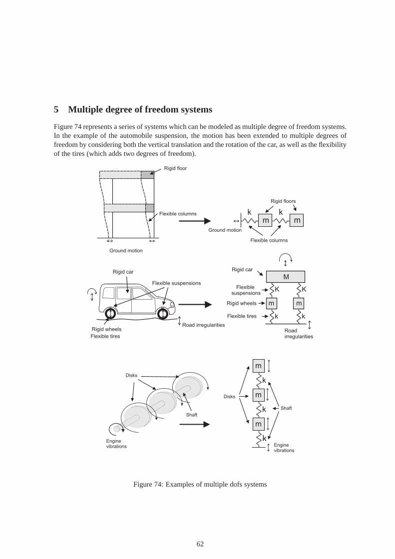
5 Multiple degree of freedom systems

Figure 74 represents a series of systems which can be modeledas multiple degree of freedom systems.In the example of the automobile suspension, the motion has been extended to multiple degrees offreedom by considering both the vertical translation and the rotation of the car, as well as the flexibilityof the tires (which adds two degrees of freedom).

Ground motion

Rigid floor

Flexible columns k km m

Ground motion

Flexible columns

Rigid floors

k

K

k

K

m

Flexible suspensions

Rigid car

Flexiblesuspensions

Rigid car

Rigid wheelsRoad irregularities

Roadirregularities

M

m

Flexible tires

Rigid wheels

Flexible tires

k

k

k

m

m

m

Disks

Enginevibrations

Shaft

Disks

Shaft

Enginevibrations

Figure 74: Examples of multiple dofs systems

62

5.1 Response of a multiple degrees of freedom system withoutdamping

Let us consider the two dofs system represented in Figure 75.A forcef is applied to the second mass.The first law of Newton is applied to each mass:

mx1 = −kx1 − k (x1 − x2) (24)

mx2 = k (x1 − x2)− kx2 + f (25)

k

kk(x -x )1 2

k kx2

mm

mm

x2

x1

x

ff

kx1

Figure 75: Forces acting on a two dofs system with two masses and three springs

This set of equations can be written in a matrix form:

[

m 00 m

]

x1x2

+

[

2k −k−k 2k

]

x1x2

=

0f

(26)

or in a more compact formMx+Kx = F (27)

whereM is the mass matrix,K is the stiffness matrix,F is the vector of forces, andx is the vectorcontaining the dofs of the system (herex1 andx2). The form of equations in (27) can be generalizedto write the equations of motion of a system withn dofs. In such a case, the size of the matrices isnx n and the size of the vectors isn.

5.1.1 General solution of the equations of motion

The general solution of (27) can be obtained assuming

x1(t)x2(t)

=

A1

A2

ert = ψert

Equation (27) becomes:(

K + r2M)

ψ = 0

This set of equations admits a non-trivial solution if

det(K + r2M) = 0

63

The roots of the determinant are purely imaginary and appearas complex conjugate pairs (this is dueto the nature of the matricesK andM which are positive definite). They can be written

r2 = −ω2

so that equation (27) can be written:(

K − ω2M)

ψ = 0

This set of equations is an eigenvalue problem. Its solutionwill give a set of eigenvalues called theeigenfrequencies (ωi, i=1..n, wheren is the number of dofs) and the associated eigenvectorsψi calledthe mode shapes. The general solution of the equation of motion can be written as the sum of functionsin the spatial domain (the mode shapes) and oscillatory functions in the time domain (oscillations atfrequenciesωi):

x(t) =n∑

i=1

(Zi1cos(ωit) + Zi2sin(ωit))ψi

The coefficientsZij are a function of the initial conditions (displacement and velocity).

Illustration: two degrees of freedom systemThe eigenfrequencies and mode shapes of the system represented in Figure 75 satisfy the set of equa-tions:

(

K − ω2M)

ψ = 0 (28)

A non-trivial solution exists if

det(K − ω2M) = det

(

2k − ω2m −k−k 2k − ω2m

)

= 0

which leads to(2k − ω2m)(2k − ω2m)− k2 = m2ω4 − 4kmω2 + 3k2 = 0

The solutions of this second order equation (ω2 is the unknown) are:

ω21 = k/m

ω22 = 3k/m

The mode shapes associated to these two eigenfrequencies are obtained by replacingω successivelyby ω1 andω2 in the first (or the second) line of (28):

Forω21 = k/m

(

2k − k

mm

)

A1 − kA2 = 0

kA1 = kA2 ⇒ A1 = A2

Forω22 = 3k/m

(

2k − 3k

mm

)

A1 − kA2 = 0

−kA1 = kA2 ⇒ A1 = −A2

64

The two mode shapes are then given by (note that a mode shape isalways known up to a constant)

ψ1 =

11

ψ2 =

1−1

The first mode shape corresponds to a translation of the two masses in phase (there is no strainin the middle spring), while the second mode shape corresponds to a motion of the two masses inopposition of phase (Figure 76).

m m

mm

x

x2

x1

x2

x1

Mode 1 Mode 2

Figure 76: Mode shapes of the two dofs system represented in Figure 75

The general solution can be written in the form:

x1(t)x2(t)

= (Z11 cosω1t+ Z12 sinω1t)

11

+ (Z21 cosω2t+ Z22 sinω2t)

1−1

Let us assume that a zero initial velocity is imposed to the two masse (x1(0) = x2(0) = 0) andthat an initial displacement is imposed in the form of

x1(0)x2(0)

=

01mm

These four conditions allow to determine the four constantsZij. The solution is

x1(t)x2(t)

=

(

12 cosω1t− 1

2 cosω2t12cosω1t+

12cosω2t

)

(mm)

The free vibration of the two dofs system subject to these initial conditions is shown in Figure 77.The presence of two frequencies, due to the existence of two eigenfrequencies can be noticed. Asthe number of dofs increases in a system; the number of eigenfrequencies also inscreases and the freevibration contains more and more frequencies.

65

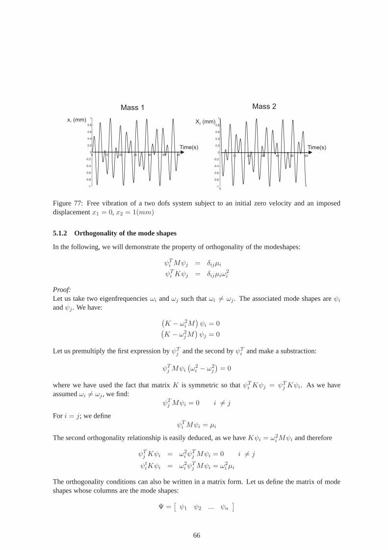
Time(s)

x (mm)1

Time(s)

X (mm)2

Mass 1 Mass 2

Figure 77: Free vibration of a two dofs system subject to an initial zero velocity and an imposeddisplacementx1 = 0, x2 = 1(mm)

5.1.2 Orthogonality of the mode shapes

In the following, we will demonstrate the property of orthogonality of the modeshapes:

ψTi Mψj = δijµi

ψTi Kψj = δijµiω

2i

Proof:Let us take two eigenfrequenciesωi andωj such thatωi 6= ωj. The associated mode shapes areψi

andψj . We have:

(

K − ω2iM)

ψi = 0(

K − ω2jM)

ψj = 0

Let us premultiply the first expression byψTj and the second byψT

i and make a substraction:

ψTj Mψi

(

ω2i − ω2

j

)

= 0

where we have used the fact that matrixK is symmetric so thatψTi Kψj = ψT

j Kψi. As we haveassumedωi 6= ωj, we find:

ψTj Mψi = 0 i 6= j

For i = j; we defineψTi Mψi = µi

The second orthogonality relationship is easily deduced, as we haveKψi = ω2iMψi and therefore

ψTj Kψi = ω2

i ψTj Mψi = 0 i 6= j

ψtiKψi = ω2

i ψTj Mψi = ω2

i µi

The orthogonality conditions can also be written in a matrixform. Let us define the matrix of modeshapes whose columns are the mode shapes:

Ψ =[

ψ1 ψ2 ... ψn

]

66

we have:

ΨTMΨ = diag(µi)

ΨTKΨ = diag(µiω2i )

wherediag(µi) is a diagonal matrix with the valuesµi on the diagonal:

diag(µi) =

µ1 0 ... 00 µ2 ... 0... ... ... ...0 0 ... µn

These relationships express the fact that the mode shapes are orthogonal with respect to the matri-cesM andK. They can therefore be used as a basis of orthogonal functions to represent the solutionof the problem.

5.1.3 Particular solution of the equation of motion

Let us start from equation (27) and decompose the solution ofthe problem in the basis of the modeshapes:

x(t) =

n∑

i=1

zi(t)ψi

which can be written in a matrix form :x = Ψz

wherez is the vector of modal amplitudes. Let us replacex byΨz in (27) and premultiply byΨT , wehave:

ΨTMΨz +ΨTKΨz = ΨT f

and using the orthogonality conditions, we find:

diag(µi)z + diag(µiω2i )z = ΨTf

which is a set ofn uncoupled equations of the type

µizi + µiω2i zi = Fi (29)

Equation (29) corresponds to the equation of motion of a single dof system with

• a massµi, called the modal mass

• a stiffnessµiω2i

• a natural frequencyωi = 2πfi

• a forceFi = ψTi f (modal excitation)

In summary, by writing the particular solutionx(t) as a function of the modal amplitudeszi(t)and the mode shapesψi, it is possible to transform the initial set ofn coupled equations into a setof n uncoupled equations. Each independent equation corresponds to the equation of motion of asingle dof system. All the tools presented in Section 3 can therefore be used to find the solution of the

67

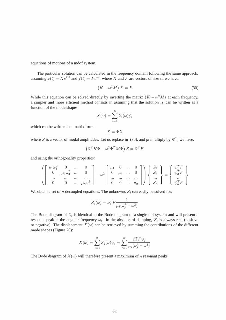
equations of motions of a mdof system.

The particular solution can be calculated in the frequency domain following the same approach,assumingx(t) = Xeiωt andf(t) = Feiωt whereX andF are vectors of sizen, we have:

(

K − ω2M)

X = F (30)

While this equation can be solved directly by inverting the matrix(

K − ω2M)

at each frequency,a simpler and more efficient method consists in assuming thatthe solutionX can be written as afunction of the mode shapes:

X(ω) =

n∑

i=1

Zi(ω)ψi

which can be written in a matrix form:X = ΨZ

whereZ is a vector of modal amplitudes. Let us replace in (30), and premultiply byΨT , we have:

(

ΨTKΨ− ω2ΨTMΨ)

Z = ΨTF

and using the orthogonality properties:

µ1ω21 0 ... 0

0 µ2ω22 ... 0

... ... ... ...0 0 ... µnω

2n

− ω2

µ1 0 ... 00 µ2 ... 0... ... ... ...0 0 ... µn

Z1

Z2

...Zn

=

ψT1 FψT2 F...ψTnF

We obtain a set ofn decoupled equations. The unknownsZi can easily be solved for:

Zj(ω) = ψTj F

1

µj(ω2j − ω2)

The Bode diagram ofZi is identical to the Bode diagram of a single dof system and will present aresonant peak at the angular frequencyωi. In the absence of damping,Zi is always real (positiveor negative). The displacementX(ω) can be retrieved by summing the contributions of the differentmode shapes (Figure 78):

X(ω) =

n∑

j=1

Zj(ω)ψj =

n∑

j=1

ψTj Fψj

µj(ω2j − ω2)

The Bode diagram ofX(ω) will therefore present a maximum ofn resonant peaks.

68

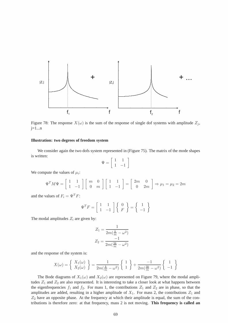
|Z |1

f1

|Z |2

f2

+ + ...

f f

Figure 78: The responseX(ω) is the sum of the response of single dof systems with amplitude Zj,j=1...n

Illustration: two degrees of freedom system

We consider again the two dofs system represented in (Figure75). The matrix of the mode shapesis written:

Ψ =

[

1 11 −1

]

We compute the values ofµi:

ΨTMΨ =

[

1 11 −1

] [

m 00 m

] [

1 11 −1

]

=

[

2m 00 2m

]

⇒ µ1 = µ2 = 2m

and the values ofFi = ΨTF :

ΨTF =

[

1 11 −1

]

0F

=

1−1

The modal amplitudesZi are given by:

Z1 =1

2m( km − ω2)

Z2 =−1

2m(3km − ω2)

and the response of the system is:

X(ω) =

X1(ω)X2(ω)

=1

2m( km − ω2)

11

+−1

2m(3km − ω2)

1−1

The Bode diagrams ofX1(ω) andX2(ω) are represented on Figure 79, where the modal ampli-tudesZ1 andZ2 are also represented. It is interesting to take a closer lookat what happens betweenthe eigenfrequenciesf1 andf2. For mass 1, the contributionsZ1 andZ2 are in phase, so that theamplitudes are added, resulting in a higher amplitude ofX1. For mass 2, the contributionsZ1 andZ2 have an opposite phase. At the frequency at which their amplitude is equal, the sum of the con-tributions is therefore zero: at that frequency, mass 2 is not moving. This frequency is called an

69

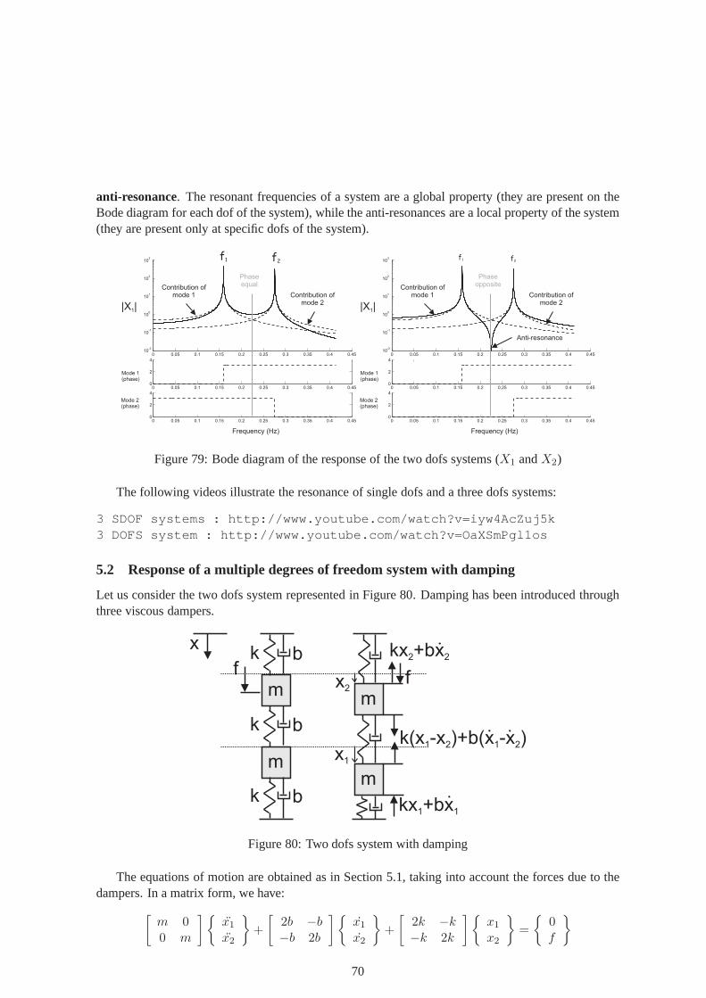
anti-resonance. The resonant frequencies of a system are a global property (they are present on theBode diagram for each dof of the system), while the anti-resonances are a local property of the system(they are present only at specific dofs of the system).

0 0.05 0.1 0.15 0.2 0.25 0.3 0.35 0.4 0.4510

-2

10-1

100

101

102

103

0 0.05 0.1 0.15 0.2 0.25 0.3 0.35 0.4 0.450

2

4

0 0.05 0.1 0.15 0.2 0.25 0.3 0.35 0.4 0.450

2

4

Frequency (Hz)

|X |1

Contribution ofmode 1

f1 f2

Mode 1(phase)

Contribution ofmode 2

Mode 2(phase)

Phaseequal

0 0.05 0.1 0.15 0.2 0.25 0.3 0.35 0.4 0.4510

-2

10-1

100

101

102

103

0 0.05 0.1 0.15 0.2 0.25 0.3 0.35 0.4 0.450

2

4

0 0.05 0.1 0.15 0.2 0.25 0.3 0.35 0.4 0.450

2

4

Frequency (Hz)

|X |1

Contribution ofmode 1

Mode 1(phase)

Contribution ofmode 2

Mode 2(phase)

Phaseopposite

Anti-resonance

f1 f2

Figure 79: Bode diagram of the response of the two dofs systems (X1 andX2)

The following videos illustrate the resonance of single dofs and a three dofs systems:

3 SDOF systems : http://www.youtube.com/watch?v=iyw4AcZuj5k3 DOFS system : http://www.youtube.com/watch?v=OaXSmPgl1os

5.2 Response of a multiple degrees of freedom system with damping

Let us consider the two dofs system represented in Figure 80.Damping has been introduced throughthree viscous dampers.

k(x -x )+b1 2 (x -x )1 2

k

k

k

kx +bx2 2

mm

mm

x2

x1

x

ff

kx +b1 x1

b

b

b

Figure 80: Two dofs system with damping

The equations of motion are obtained as in Section 5.1, taking into account the forces due to thedampers. In a matrix form, we have:

[

m 00 m

]

x1x2

+

[

2b −b−b 2b

]

x1x2

+

[

2k −k−k 2k

]

x1x2

=

0f

70

which can be written in a compact form

Mx+ Cx+Kx = f (31)

whereC is the damping matrix.

5.2.1 General solution of the equations of motion

The general solution of the equations of motion of a damped mdof system can be obtained by posing

x1(t)x2(t)

=

A1

A2

ert = ψert

Equation (31) becomes(

K + rC + r2M)

ψ = 0

which admits non-trivial solutions for the roots of

det(K + rC + r2M) = 0

The roots of this determinant are complex, and the free response is characterised by oscillatory func-tions with an exponentially decaying envelope in the time domain. The associated eigenvectors arealso complex, which means that their different components are not in phase. As it is not very commonto use complex mode shapes in structural dynamics, we will not discuss them in further details.

5.2.2 Particular solution of the equations of motion

An alternative to the use of complex mode shapes is to calculate the response of the system using thereal mode shapes associated to theK andM matrices. Let us start from equation (31) and decomposethe solution of the problem in the basis of the mode shapes:

x(t) =

n∑

i=1

zi(t)ψi

which can be written in a matrix form :x = Ψz

wherez is the vector of modal amplitudes. Let us replacex byΨz in (31) and premultiply byΨT , wehave:

ΨTMΨz +ΨTCΨz +ΨTKΨz = ΨT f

In general, the termΨTCΨ is not diagonal and the equations remain coupled. An approximation canbe obtained however in the following cases:

• Rayleigh damping: this damping model assumes that the matric C can be written as:

C = αK + βM

In such a case, the termΨTCΨ reduces to:

ΨTCΨ = ΨT (αK + βM)Ψ = diag(αµiω2i + βµi)

This model is often used as an approximation in order to decouple the equations, but the modelhas no physical meaning.

71

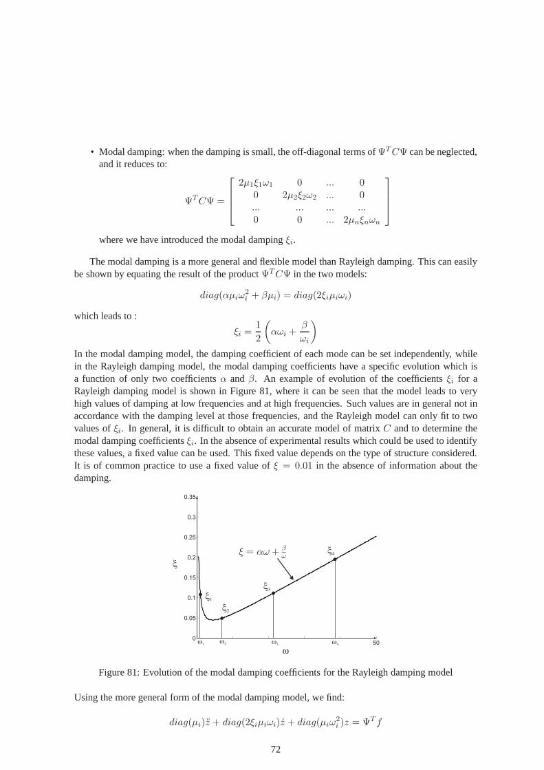
• Modal damping: when the damping is small, the off-diagonalterms ofΨTCΨ can be neglected,and it reduces to:

ΨTCΨ =

2µ1ξ1ω1 0 ... 00 2µ2ξ2ω2 ... 0... ... ... ...0 0 ... 2µnξnωn

where we have introduced the modal dampingξi.

The modal damping is a more general and flexible model than Rayleigh damping. This can easilybe shown by equating the result of the productΨTCΨ in the two models:

diag(αµiω2i + βµi) = diag(2ξiµiωi)

which leads to :

ξi =1

2

(

αωi +β

ωi

)

In the modal damping model, the damping coefficient of each mode can be set independently, whilein the Rayleigh damping model, the modal damping coefficients have a specific evolution which isa function of only two coefficientsα andβ. An example of evolution of the coefficientsξi for aRayleigh damping model is shown in Figure 81, where it can be seen that the model leads to veryhigh values of damping at low frequencies and at high frequencies. Such values are in general not inaccordance with the damping level at those frequencies, andthe Rayleigh model can only fit to twovalues ofξi. In general, it is difficult to obtain an accurate model of matrix C and to determine themodal damping coefficientsξi. In the absence of experimental results which could be used to identifythese values, a fixed value can be used. This fixed value depends on the type of structure considered.It is of common practice to use a fixed value ofξ = 0.01 in the absence of information about thedamping.

500

0.05

0.1

0.15

0.2

0.25

0.3

0.35

w

x

ø = ë!+ !ì

x1

x2

x3

x4

w1w2 w3 w4

Figure 81: Evolution of the modal damping coefficients for the Rayleigh damping model

Using the more general form of the modal damping model, we find:

diag(µi)z + diag(2ξiµiωi)z + diag(µiω2i )z = ΨT f

72

which is a set ofn uncoupled equations of the type

µizi + 2ξiµiωiz + µiω2i zi = Fi (32)

Equation (32) corresponds to the equation of motion of a damped single dof system with

• a massµi, called the modal mass

• a stiffnessµiω2i

• a damping coefficientξi

• a natural frequencyωi = 2πfi

• a forceFi = ψTi f (modal excitation)

The particular solution can be calculated in the frequency domain following the same approach,assumingx(t) = Xeiωt andf(t) = Feiωt whereX andF are complex vectors of sinen, we have:

(

K + iωC − ω2M)

X = F (33)

the solutionX is written as a function of the mode shapes:

X(ω) =

n∑

j=1

Zj(ω)ψj

which can be written in a matrix form:X = ΨZ

whereZ is a complex vector of modal amplitudes. Let us replace in (30), and premultiply byΨT , wehave:

(

ΨTKΨ+ iωΨTCΨ− ω2ΨTMΨ)

Z = ΨTF

and using the orthogonality properties and the modal damping model:

µj(ω2j − ω2 + 2iξjωωj)Zj = Fj

We obtain a set ofn decoupled equations. The unknownsZj can easily be solved for:

Zj(ω) =ψTj F

µj(ω2j − ω2 + 2iξjωωj)

The Bode diagram ofZi is identical to the Bode diagram of a damped single dof systemand willpresent a damped resonant peak at the angular frequencyωi. Due to the damping,Zi is complex. ThedisplacementX(ω) can be retrieved by summing the contributions of the different mode shapes:

X(ω) =n∑

j=1

Zj(ω)ψj =n∑

j=1

ψTj Fψj

µj(ω2j − ω2) + 2iξjωωj

73

Illustration: two degrees of freedom systemLet us consider the system represented in Figure 80, and takethe following values for the differentcoefficients:k = 1N/m,m = 1kg andb = 0.04Ns/m. In the present case, matrixC is proportionnalto matrixK and the productΨTCΨ is diagonal. We calculate the valus ofξj : ξ1 = 2% andξ2 =3.5%. The forced response of mass 2 as a function of the frequency is represented on Figure 82. Notethat the second peak is more damped than the first one due to thefact thatξ2 > ξ1.

Frequency(Hz)

f(°)

|X /F|2

x1=2%

x2=3.5%

Figure 82: Bode diagram for mass 2 of the two dofs system with adamping matrix propotionnal tothe stiffness matrix

Let us now remove the damper between mass 1 and the ground (Figure 83). MatrixC is notproportional to matrixK anymore so that the productΨTCΨ is not diagonal. Let us neglect the off-diagonal terms and compute the modal damping coefficients. We getξ1 = 1% eandξ2 = 2.9%. OnFigure 84, the Bode diagram for mass 2 is plotted and the solution found neglecting the off-diagonalterms is compared to the solution obtained with the coupled equations (no terms neglected). Thefigure shows that the solutions are almost identical. It is therefore justified to neglect the off-diagonalterms because the damping is small.

k

k

k

m

m

x

fb

b

Figure 83: Two dofs system with damping - the viscous damper between the ground and mass 1 hasbeen removed

74

0 0.05 0.1 0.15 0.2 0.25 0.3 0.35 0.4 0.4510

-2

10-1

100

101

102

0 0.05 0.1 0.15 0.2 0.25 0.3 0.35 0.4 0.45-4

-3

-2

-1

0

Frequency(Hz)

f(°)

|X /F|2

x1=1%

x2=2.9%

Exact

Modal damping

Figure 84: Bode diagram for mass 2 of the two dofs system with anon-proportionnal damping:comparison between the exact solution and the approximation using the modal damping model for alow value of damping

Let us now assume that the damping coefficient isb = 0.2Ns/m. The modal damping coefficientsareξ1 = 5% et ξ2 = 14.43% which cannot be considered as small damping anymore. In thiscase, asshown in Figure 85, the modal damping model deviates from theexact solution.

0 0.05 0.1 0.15 0.2 0.25 0.3 0.35 0.4 0.45

100

0 0.05 0.1 0.15 0.2 0.25 0.3 0.35 0.4 0.45-3

-2

-1

0

Frequency(Hz)

f(°)

x1=5%

x2=14.43%|X /F|2

Figure 85: Bode diagram for mass 2 of the two dofs system with anon-proportionnal damping:comparison between the exact solution and the approximation using the modal damping model for ahigh value of damping

5.3 MDOF application: the tuned mass damper

A tuned mass damper (TMD) is a device that it attached to a primary structure in order to damp itsvibrations. The first type of tuned mass damper we are going tostudy is a mass-spring system . In this

75

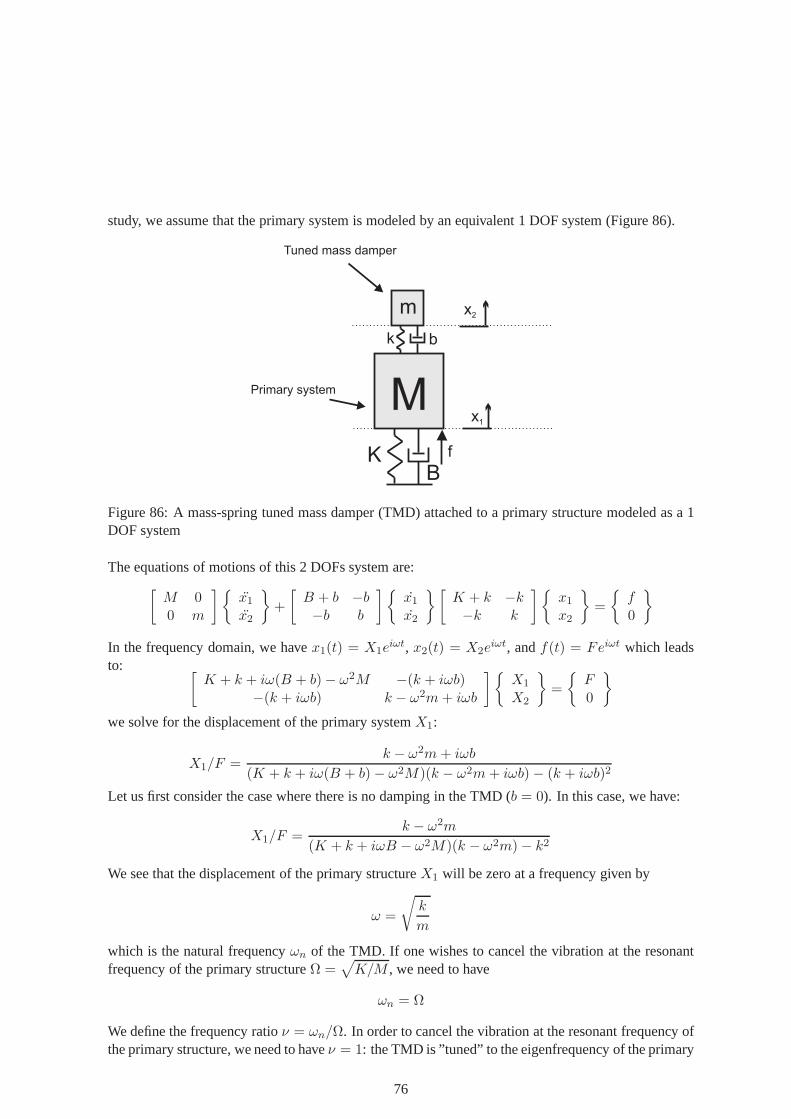
study, we assume that the primary system is modeled by an equivalent 1 DOF system (Figure 86).

k

MfK

m

x1

x2

Tuned mass damper

Primary system

B

b

Figure 86: A mass-spring tuned mass damper (TMD) attached toa primary structure modeled as a 1DOF system

The equations of motions of this 2 DOFs system are:[

M 00 m

]

x1x2

+

[

B + b −b−b b

]

x1x2

[

K + k −k−k k

]

x1x2

=

f0

In the frequency domain, we havex1(t) = X1eiωt, x2(t) = X2e

iωt, andf(t) = Feiωt which leadsto:

[

K + k + iω(B + b)− ω2M −(k + iωb)−(k + iωb) k − ω2m+ iωb

]

X1

X2

=

F0

we solve for the displacement of the primary systemX1:

X1/F =k − ω2m+ iωb

(K + k + iω(B + b)− ω2M)(k − ω2m+ iωb)− (k + iωb)2

Let us first consider the case where there is no damping in the TMD (b = 0). In this case, we have:

X1/F =k − ω2m

(K + k + iωB − ω2M)(k − ω2m)− k2

We see that the displacement of the primary structureX1 will be zero at a frequency given by

ω =

√

k

m

which is the natural frequencyωn of the TMD. If one wishes to cancel the vibration at the resonantfrequency of the primary structureΩ =

√

K/M , we need to have

ωn = Ω

We define the frequency ratioν = ωn/Ω. In order to cancel the vibration at the resonant frequency ofthe primary structure, we need to haveν = 1: the TMD is ”tuned” to the eigenfrequency of the primary

76

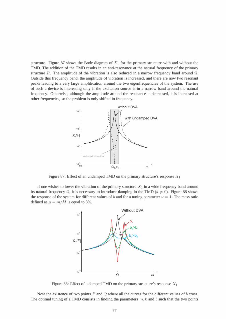
structure. Figure 87 shows the Bode diagram ofX1 for the primary structure with and without theTMD. The addition of the TMD results in an anti-resonance at the natural frequency of the primarystructureΩ. The amplitude of the vibration is also reduced in a narrow frequency band aroundΩ.Outside this frequency band, the amplitude of vibration is increased, and there are now two resonantpeaks leading to a very large amplification around the two eigenfrequencies of the system. The useof such a device is interesting only if the excitation sourceis in a narrow band around the naturalfrequency. Otherwise, although the amplitude around the resonance is decreased, it is increased atother frequencies, so the problem is only shifted in frequency.

0.510

-1

100

101

102

without DVA

W w1= 1

with undamped DVA

reduced vibration

|X1

w

/F|

Figure 87: Effect of an undamped TMD on the primary structure’s responseX1

If one wishes to lower the vibration of the primary structureX1 in a wide frequency band aroundits natural frequencyΩ, it is necessary to introduce damping in the TMD (b 6= 0). Figure 88 showsthe response of the system for different values ofb and for a tuning parameterν = 1. The mass ratiodefined asµ = m/M is equal to 3%.

10-1

100

101

102

Without DVA

P Q

b1

b >b2 1

b >b3 2

W

|X1

w

/F|

Figure 88: Effect of a damped TMD on the primary structure’s responseX1

Note the existence of two pointsP andQ where all the curves for the different values ofb cross.The optimal tuning of a TMD consists in finding the parametersm,k andb such that the two points

77

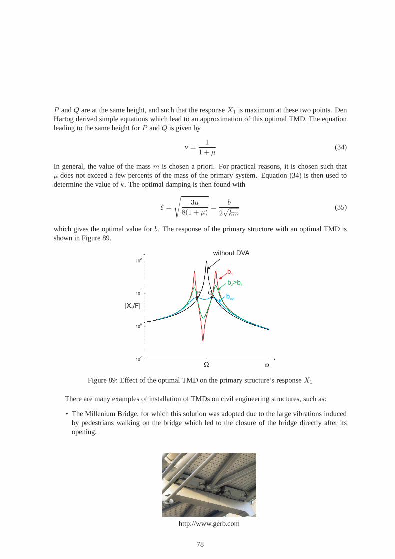
P andQ are at the same height, and such that the responseX1 is maximum at these two points. DenHartog derived simple equations which lead to an approximation of this optimal TMD. The equationleading to the same height forP andQ is given by

ν =1

1 + µ(34)

In general, the value of the massm is chosen a priori. For practical reasons, it is chosen such thatµ does not exceed a few percents of the mass of the primary system. Equation (34) is then used todetermine the value ofk. The optimal damping is then found with

ξ =

√

3µ

8(1 + µ)=

b

2√km

(35)

which gives the optimal value forb. The response of the primary structure with an optimal TMD isshown in Figure 89.

10-1

100

101

102

without DVA

P

b1

b >b2 1

bopt

Q

W

|X /F|1

w

Figure 89: Effect of the optimal TMD on the primary structure’s responseX1

There are many examples of installation of TMDs on civil engineering structures, such as:

• The Millenium Bridge, for which this solution was adopted due to the large vibrations inducedby pedestrians walking on the bridge which led to the closureof the bridge directly after itsopening.

http://www.gerb.com

78

• The John Hancock Tower in Boston (1976), where two TMDs consisting of large steel blocksof approx 5.2x5.2x1m (weighting 270 Tons) were installed atthe top of the tower (tuned to 0.14Hz).

http://www.lemessurier.com

• The city corp Center in New York (1977), where 1 TMD of 400 Tons acting in two directionshas been installed (tuned to 0.16 Hz).

http://www.estructura.it

• The Chiba Port Tower (Japan - 1986), where 1 TMD of 15 Tons acting in two directions hasbeen installed (0.44 Hz).

http://www.iitk.ac.in

79

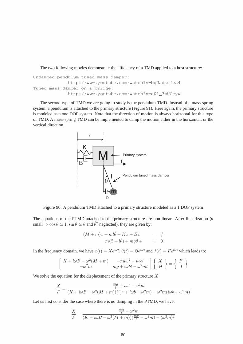
The two following movies demonstrate the efficiency of a TMD applied to a host structure:

Undamped pendulum tuned mass damper:http://www.youtube.com/watch?v=bqJadkufes4

Tuned mass damper on a bridge:http://www.youtube.com/watch?v=e01_3mUGeyw

The second type of TMD we are going to study is the pendulum TMD. Instead of a mass-springsystem, a pendulum is attached to the primary structure (Figure 91). Here again, the primary structureis modeled as a one DOF system. Note that the direction of motion is always horizontal for this typeof TMD. A mass-spring TMD can be implemented to damp the motion either in the horizontal, or thevertical direction.

Mf

K

Pendulum tuned mass damper

Primary system

x

m

ql

b

B

Figure 90: A pendulum TMD attached to a primary structure modeled as a 1 DOF system

The equations of the PTMD attached to the primary structure are non-linear. After linearization (θsmall⇒ cos θ ≃ 1, sin θ ≃ θ andθ2 neglected), they are given by:

(M +m)x+mlθ +Kx+Bx = f

m(x+ lθ) +mgθ + = 0

In the frequency domain, we havex(t) = Xeiωt, θ(t) = Θeiωt andf(t) = Feiωt which leads to:

[

K + iωB − ω2(M +m) −mlω2 − iωbl−ω2m mg + iωbl − ω2ml

]

XΘ

=

F0

We solve the equation for the displacement of the primary structureX

X

F=

mgl + iωb− ω2m

(K + iωB − ω2(M +m))(mgl + iωb− ω2m)− ω2m(iωb+ ω2m)

Let us first consider the case where there is no damping in the PTMD, we have:

X

F=

mgl − ω2m

(K + iωB − ω2(M +m))(mgl − ω2m)− (ω2m)2

80

Let us define

ωn =

√

g

l

which is the eigenfrequency of the undamped TMD and

Ω =

√

K

M

which is the eigenfrequency of the primary structure without the TMD. In order to cancel the vibrationat the eigenfrequency of the primary structure, we need to haveν = 1 where

ν =ωn

Ω

Figure 91 shows the response of the primary structureX with and without PTMD (ν = 1) and forseveral values of the mass of the pendulum. Note that the eigenfrequency of a pendulum only dependson its length, and not on its mass, so the tuning is not alteredwhen the mass is increased. We see thatthe two peaks are further apart as the mass increases. As in the case of the mass-spring TMD, whenthere is no damping, the vibration can be canceled at the resonant frequency of the primary structure,but we note the appearance of two peaks away from that resonant frequency. The device is thereforeonly suited when one wants to decrease the vibration in a narrow frequency band around the resonance(the frequency band can be made larger if one increases the mass of the PTMD).

10-3

10-2

10-1

100

101

102

without PTMD

m1

W

m >m2 1

w

|X1/F|

Figure 91: Response of the primary structure to which and undamped PTMD is attached

Let us now consider the case of the damped PTMD. As the equations are different from the mass-spring TMD, we cannot apply equations (34) and (35). The firsttuning rule is given by:

ν =

√

2

(2 + 3µ)(1 + 2µ)

The second rule is much more complex and given by:

r =

√2√µ√

3√µ√

3µ2 + 4µ + 1√3µ+ 2− 9µ2 − 11µ − 3

√

−3µ2 − 5µ+√µ√

3µ2 + 4µ+ 1√3µ + 2− 2

√3µ+ 2 (4µ + 2)

81

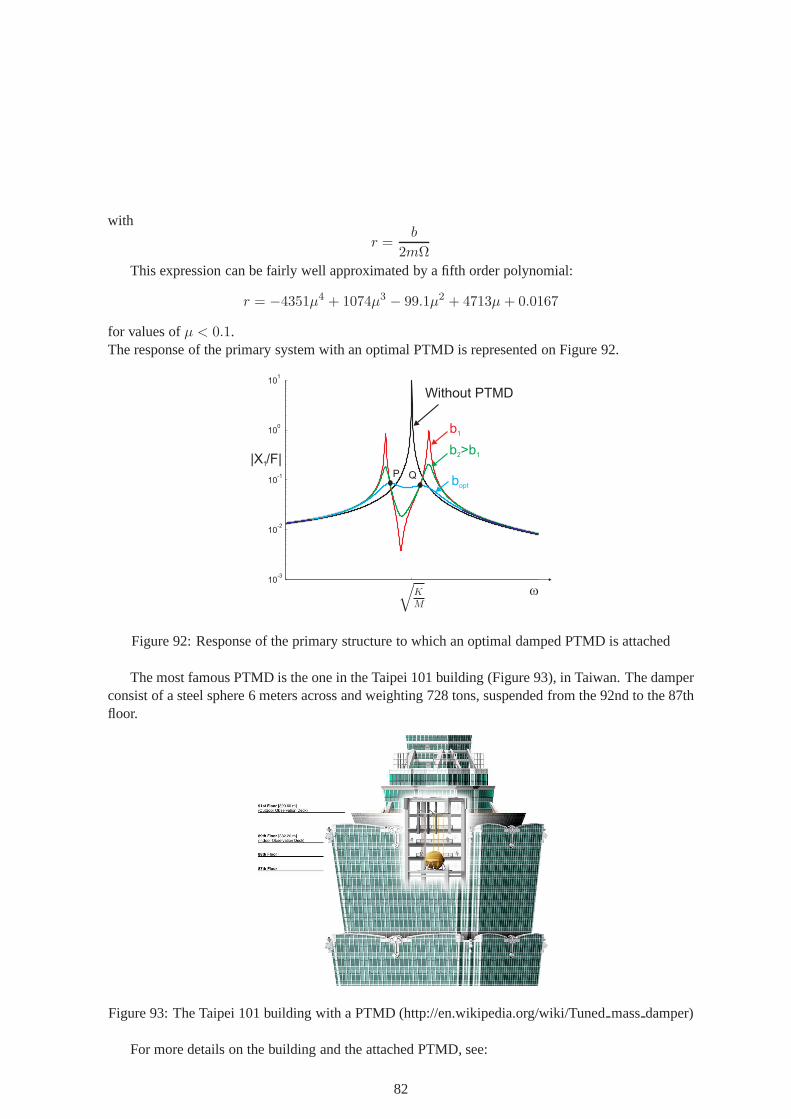
with

r =b

2mΩ

This expression can be fairly well approximated by a fifth order polynomial:

r = −4351µ4 + 1074µ3 − 99.1µ2 + 4713µ + 0.0167

for values ofµ < 0.1.The response of the primary system with an optimal PTMD is represented on Figure 92.

10-3

10-2

10-1

100

101

Without PTMD

P

b1

b >b2 1

bopt

MK

q

Q

w

|X1/F|

Figure 92: Response of the primary structure to which an optimal damped PTMD is attached

The most famous PTMD is the one in the Taipei 101 building (Figure 93), in Taiwan. The damperconsist of a steel sphere 6 meters across and weighting 728 tons, suspended from the 92nd to the 87thfloor.

Figure 93: The Taipei 101 building with a PTMD (http://en.wikipedia.org/wiki/Tunedmassdamper)

For more details on the building and the attached PTMD, see:

82

Taipei Discovery Channel: http://www.youtube.com/watch?v=xF7foZ-oiSoTaipei 101 sketch of pendulum: http://www.youtube.com/watch?v=uybEXOkkrswTaipei TMD Motion on May 12, 2008 : http://www.youtube.com/watch?v=NYSgd1XSZXc

Additional movies (not played in class)

Citicorp Centerhttp://www.youtube.com/watch?v=TZhgTewKhTQhttp://www.youtube.com/watch?v=4fUwgH0gOWohttp://www.youtube.com/watch?v=IBjyB8EY2m4#t=2

83

6 Continuous systems

In the previous chapters, we have studied systems which can be simplified and modeled as massesconnected with springs and dampers. In the real world, structures are always continuous. Somecontinuous structures can be simplified and be modeled as beams or bars, while others cannot. Inthe first part of this section, we will discuss the computation of the dynamic response of bars andbeams. The second part will be devoted to the computation of the dynamic response of more generalcontinuous structures. A continuous system can be seen as the limit whenn tends to infinity of andofs system. A continuous system therefore has an infinite number of eigenfrequencies and modeshapes.

6.1 Beams and bars

6.1.1 Boundary conditions for beams and bars

If we consider a bar in traction, the displacement is in thex direction (Figure 94). Atx = 0 andx = L, the bar can either be free or fixed. A fixed condition corresponds tox = 0, while a freecondition corresponds to the absence of an applied normal forceN = Eε = E du

dx , which we usuallysimplify to u′ = du

dx=0 (Figure 95).

u(x)

x

Figure 94: Bar in traction: the displacement is in thex direction

N=0 -> u’=0u=0

Figure 95: Boundary conditions for bars in traction

If we consider a beam in bending, the displacement is in they direction (Figure 96). Atx = 0andx = L, there are four possible boundary conditions. The first two boundary conditions are linkedto the vertical displacement which is either fixed (y = 0) or free (the shear forceT = −EIyIII = 0,which can be simplified toyIII = 0), while the second set of boundary conditions is linked to therotation which is either fixed (y′ = 0) or free (the bending momentM = −EIy′′ = 0, which can besimplified toy′′ = 0) (Figure 97).

y(x)

x

Figure 96: Bar in bending: the displacement is in they direction

84

M=0 -> y’’=0T=0 -> y’’’=0

M=0 -> y’’=0y=0

y=0

=0 -> y’=0q

Figure 97: Boundary conditions for beams in bending

6.1.2 Bar in traction: equation of motion

The equation of motion for a bar in traction can be found by isolating a small part of the bar of lengthdx as shown in Figure 98:

−N + p(x, t) dx +N + dN = (ρAu(x, t)) dx

wherep(x, t) is the load per unit of length in directionx, ρ is the density of the material (kg/m3) andA is the area of the section of the bar. This expression leads to

dN

dx=

∂

∂x

(

EA∂u

∂x

)

= EA∂2u(x, t)

∂x2= ρAu(x, t)− p(x, t)

assumingEA is constant. We therefore have

EA∂2u(x, t)

∂x2− ρAu(x, t) = −p(x, t) (36)

dx

N+dNNp(x,t)

x

u(x,t)

L

Figure 98: Equilibrium of a small part of a bar of lengthdx

6.1.3 Bar in traction: mode shapes and eigenfrequencies

Assumingu(x, t) = U(x)eiωt, the mode shapes and eigenfrequencies are the solution of the equationof motion with the right-hand side equal to 0:

EAd2U

dx2+ ρAω2U = 0

which can be rewrittend2U

dx2+ρ

Eω2U = 0

85

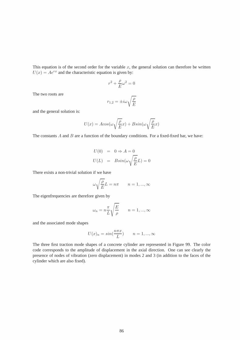
This equation is of the second order for the variablex, the general solution can therefore be writtenU(x) = Aerx and the characteristic equation is given by:

r2 +ρ

Eω2 = 0

The two roots are

r1,2 = ±iω√

ρ

E

and the general solution is:

U(x) = Acos(ω

√

ρ

Ex) +Bsin(ω

√

ρ

Ex)

The constantsA andB are a function of the boundary conditions. For a fixed-fixed bar, we have:

U(0) = 0 ⇒ A = 0

U(L) = Bsin(ω

√

ρ

EL) = 0

There exists a non-trivial solution if we have

ω

√

ρ

EL = nπ n = 1, ...,∞

The eigenfrequencies are therefore given by

ωn = nπ

L

√

E

ρn = 1, ...,∞

and the associated mode shapes

U(x)n = sin(nπx

L) n = 1, ...,∞

The three first traction mode shapes of a concrete cylinder are represented in Figure 99. The colorcode corresponds to the amplitude of displacement in the axial direction. One can see clearly thepresence of nodes of vibration (zero displacement) in modes2 and 3 (in addition to the faces of thecylinder which are also fixed).

86

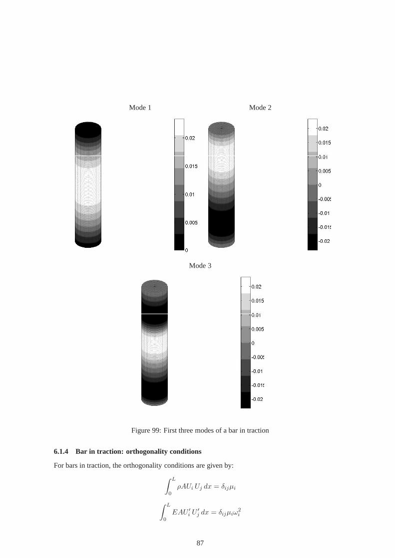
Mode 1 Mode 2

Mode 3

Figure 99: First three modes of a bar in traction

6.1.4 Bar in traction: orthogonality conditions

For bars in traction, the orthogonality conditions are given by:

∫ L

0ρAUi Uj dx = δijµi

∫ L

0EAU ′

i U′j dx = δijµiω

2i

87

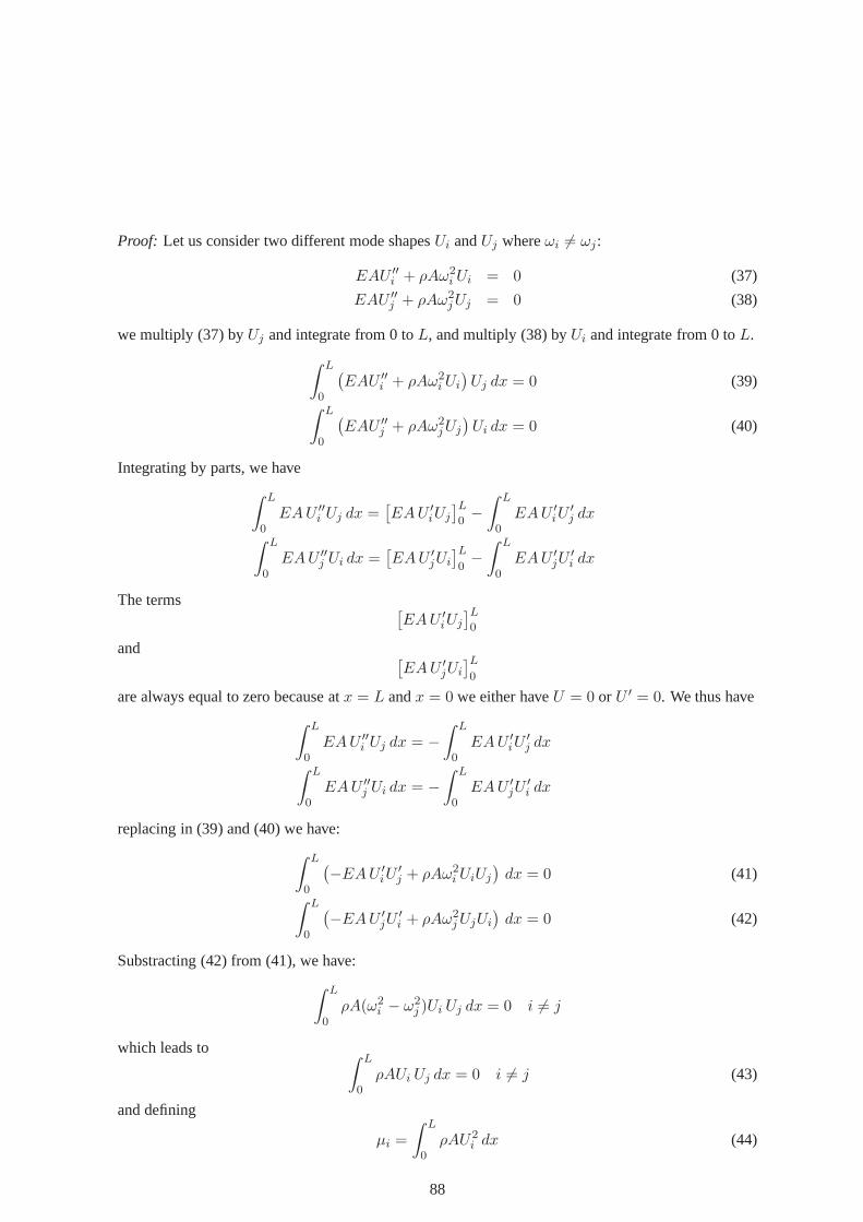
Proof: Let us consider two different mode shapesUi andUj whereωi 6= ωj:

EAU ′′i + ρAω2

i Ui = 0 (37)

EAU ′′j + ρAω2

jUj = 0 (38)

we multiply (37) byUj and integrate from 0 toL, and multiply (38) byUi and integrate from 0 toL.

∫ L

0

(

EAU ′′i + ρAω2

iUi

)

Uj dx = 0 (39)

∫ L

0

(

EAU ′′j + ρAω2

jUj

)

Ui dx = 0 (40)

Integrating by parts, we have

∫ L

0EAU ′′

i Uj dx =[

EAU ′iUj

]L

0−∫ L

0EAU ′

iU′j dx

∫ L

0EAU ′′

j Ui dx =[

EAU ′jUi

]L

0−∫ L

0EAU ′

jU′i dx

The terms[

EAU ′iUj

]L

0

and[

EAU ′jUi

]L

0

are always equal to zero because atx = L andx = 0 we either haveU = 0 or U ′ = 0. We thus have

∫ L

0EAU ′′

i Uj dx = −∫ L

0EAU ′

iU′j dx

∫ L

0EAU ′′

j Ui dx = −∫ L

0EAU ′

jU′i dx

replacing in (39) and (40) we have:

∫ L

0

(

−EAU ′iU

′j + ρAω2

i UiUj

)

dx = 0 (41)

∫ L

0

(

−EAU ′jU

′i + ρAω2

jUjUi

)

dx = 0 (42)

Substracting (42) from (41), we have:

∫ L

0ρA(ω2

i − ω2j )Ui Uj dx = 0 i 6= j

which leads to∫ L

0ρAUi Uj dx = 0 i 6= j (43)

and defining

µi =

∫ L

0ρAU2

i dx (44)

88

(43) and (44) give the second orthogonality condition. We can rewrite (41):

∫ L

0EAU ′

iU′j dx =

∫ L

0ρAω2

i UiUjdx

and taking into account (43) and (44), we have:

∫ L

0EAU ′

iU′j dx = 0 i 6= j

∫ L

0EAU ′2

i dx = ω2i µi

which is the first orthogonality condition.

6.1.5 Bar in traction: projection in the modal basis

Starting from the equation of motion

EA∂2u(x, t)

∂x2− ρA

∂2u(x, t)

∂t2= −p(x, t)

we assume that the solution can be written as a function of themode shapes:

u(x, t) =

∞∑

i=1

Ui(x)zi(t)

Plugging in the equation of motion, we get:

EA∞∑

i=1

U ′′i zi − ρA

∞∑

i=1

Uizi = −p(x, t)

We multiply byUj and integrate from 0 toL:

∫ L

0

(

EA∞∑

i=1

U ′′i zi

)

Uj dx−∫ L

0

(

ρA∞∑

i=1

Uizi

)

Uj dx =

∫ L

0−p(x, t)Uj dx

and rearranging:

∫ L

0

(

EA∞∑

i=1

U ′′i Uj

)

zi dx−∫ L

0

(

ρA∞∑

i=1

UiUj

)

zi dx =

∫ L

0−p(x, t)Uj dx

We can then use the orthogonality conditions to have

µizi + µiω2i zi = Fi (45)

with

Fi =

∫ L

0p(x, t)Ui dx

Equation (45) is the equation of motion of a one dof system where

89

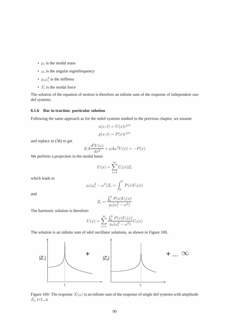
• µi is the modal mass

• ωi is the angular eigenfrequency

• µiω2i is the stiffness

• Fi is the modal force

The solution of the equation of motion is therefore an infinite sum of the response of independent onedof systems.

6.1.6 Bar in traction: particular solution

Following the same approach as for the mdof systems studied in the previous chapter, we assume

u(x, t) = U(x)eiωt

p(x, t) = P (x)eiωt

and replace in (36) to get

EAd2U(x)

dx2+ ρAω2U(x) = −P (x)

We perform a projection in the modal basis:

U(x) =∞∑

i=1

Ui(x)Zi

which leads to

µi(ω2i − ω2)Zi =

∫ L

0P (x)Ui(x)

and

Zi =

∫ L0 P (x)Ui(x)

µi(ω2i − ω2)

The harmonic solution is therefore:

U(x) =

∞∑

i=1

∫ L0 P (x)Ui(x)

µi(ω2i − ω2)

Ui(x)

The solution is an infinite sum of sdof oscillator solutions,as shown in Figure 100.

|Z |1

f1

|Z |2

f2

+ + ... 1

Figure 100: The responseX(ω) is an infinite sum of the response of single dof systems with amplitudeZi, i=1...n

90

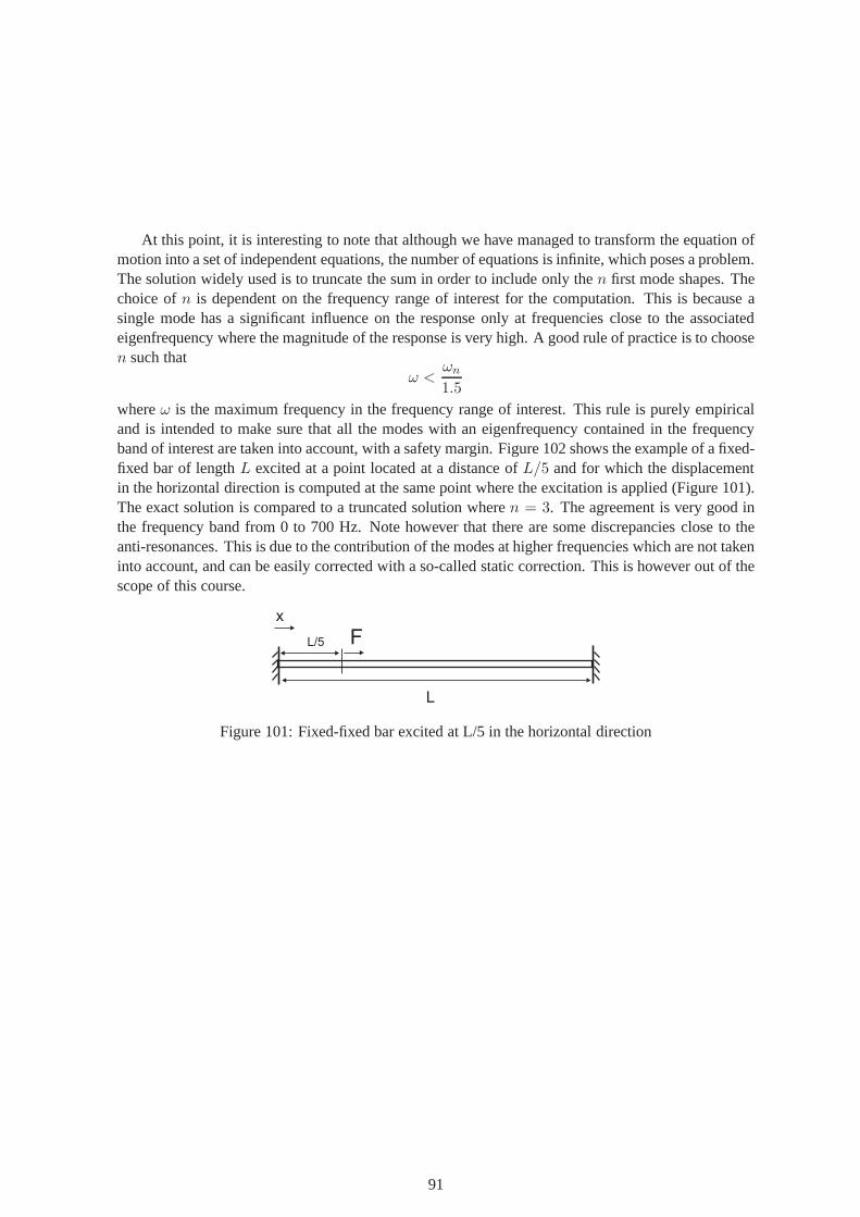
At this point, it is interesting to note that although we havemanaged to transform the equation ofmotion into a set of independent equations, the number of equations is infinite, which poses a problem.The solution widely used is to truncate the sum in order to include only then first mode shapes. Thechoice ofn is dependent on the frequency range of interest for the computation. This is because asingle mode has a significant influence on the response only atfrequencies close to the associatedeigenfrequency where the magnitude of the response is very high. A good rule of practice is to choosen such that

ω <ωn

1.5

whereω is the maximum frequency in the frequency range of interest.This rule is purely empiricaland is intended to make sure that all the modes with an eigenfrequency contained in the frequencyband of interest are taken into account, with a safety margin. Figure 102 shows the example of a fixed-fixed bar of lengthL excited at a point located at a distance ofL/5 and for which the displacementin the horizontal direction is computed at the same point where the excitation is applied (Figure 101).The exact solution is compared to a truncated solution wheren = 3. The agreement is very good inthe frequency band from 0 to 700 Hz. Note however that there are some discrepancies close to theanti-resonances. This is due to the contribution of the modes at higher frequencies which are not takeninto account, and can be easily corrected with a so-called static correction. This is however out of thescope of this course.

x

F

L

L/5

Figure 101: Fixed-fixed bar excited at L/5 in the horizontal direction

91

0 200 400 600 800 100010

-11

10-10

10-9

10-8

10-7

10-6

Frequency (Hz)

u(L

/5)/

F (

dB

)Exact Truncated

Figure 102: Comparison between the exact solution and a solution obtained by truncating the expan-sion in the modal basis to the third mode

6.1.7 Bar in traction: comparison with mdof systems

MDOF systems Bar in tractionOrthogonality conditions

ψTi Mψj = δijµi

∫ L

0ρAUi Uj dx = δijµi

ψTi Kψj = δijµiω

2i

∫ L

0EAU ′

i U′j dx = δijµiω

2i

Projection in the modal basis

µizi + µiω2i zi = Fi

Fi = ΨTF Fi =

∫ L

0p(x, t)Ui dx

Response to harmonic excitation

X(ω) =

n∑

i=1

ψTi F

µi(ω2i − ω2)

ψi U(x) =

∞∑

i=1

∫ L0 P (x)Ui(x)

µi(ω2i − ω2)

Ui(x)

92

6.1.8 Beam in bending: equation of motion

The equation of motion for a beam in bending can be found by isolating a small part of the bar oflengthdx as shown in Figure 103:

−T + p(x, t) dx+ T + dT = (ρAy) dx

wherep(x) is the vertical charge per unit of length. We know thatT = −EIyIII so that the equationof motion can be rewritten:

dT

dx= −EI d

4y

dx4= ρAy − p(x, t)

or

EId4y

dx4+ ρAy = p(x, t)

dx

T+dTTp(x,t)x

y(x,t)

L

Figure 103: Equilibrium of a small part of a beam of lengthdx

6.1.9 Beam in bending: mode shapes and eigenfrequencies

Assumingy(x, t) = Y (x)eiωt, the mode shapes and eigenfrequencies are the solution of the equationof motion with the right-hand side equal to 0:

EId4Y

dx4− ρAω2Y = 0

which can be rewritten:d4Y

dx4− ρA

EIω2Y = 0

Let us define

ξ4 =ρA

EIω2

we haved4Y

dx4− ξ4Y = 0

The characteristic equation is given by:r4 + ξ4 = 0

It admits four roots

r1,2 = ±iξr3,4 = ±ξ

93

and the general solution is written in the form

Y (x) = Acos(ξx) +Bsin(ξx) + Ccosh(ξx) +Dsinh(ξx)

The constantsA,B,C andD depend on the boundary conditions

For a simply supported beam we have:

Y (0) = A+ C = 0 ⇒ C = −AY ′′(0) = ξ2 (−A+ C) = 0 ⇒ A = 0, C = 0

The solution therefore reduces to

Y (x) = Bsinξx+Dsinhξx

and taking into account the boundary conditions atx = L we have:

Y (L) = B sin ξL+DsinhξL = 0 (46)

Y ′′(L) = ξ2 (−B sin ξL+DsinhξL) = 0 (47)

The system of equations admits a non trivial solution if the determinant is zero:

det

(

sin ξL sinhξL− sin ξL sinhξL

)

= 0

which leads tosin(ξL)sinh(ξL) = 0

Apart from the trivial solutionξ = 0, we have an infinite number of solutions corresponding tosin ξL = 0 which is true for

ξL = nπ n = 1...∞We have

ξ2L2 = ω

√

ρA

EIL2

with ξL = nπ which gives for the eigenfrequencies

ωn =n2π2

L2

√

EI

ρA

The mode shapes are obtained b replacingξL by nπ in (46) , which leads toD = 0, and therefore

Y (x) = sinnπx

L

Mode shapes 1,5 and 10 are represented on Figure 104. This expression is identical to the mode-shapes of a bar in traction, but the motion here is in the vertical direction. The eigenfrequencies areproportional to the square root of the ratio of the bending rigidity EI and the mass per unit of lengthρA. The difference with the bar in traction is the fact that the eigenfrequency is proportional ton for

94

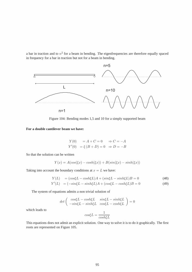
a bar in traction and ton2 for a beam in bending. The eigenfrequencies are therefore equally spacedin frequency for a bar in traction but not for a beam in bending.

L

n=1

n=5

n=10

Figure 104: Bending modes 1,5 and 10 for a simply supported beam

For a double cantilever beam we have:

Y (0) = A+ C = 0 ⇒ C = −AY ′(0) = ξ (B +D) = 0 ⇒ D = −B

So that the solution can be written

Y (x) = A(cos(ξx)− cosh(ξx)) +B(sin(ξx)− sinh(ξx))

Taking into account the boundary conditions atx = L we have:

Y (L) = (cosξL− coshξL)A+ (sinξL− sinhξL)B = 0 (48)

Y ′(L) = (−sinξL− sinhξL)A+ (cosξL− coshξL)B = 0 (49)

The system of equations admits a non trivial solution of

det

(

cosξL− coshξL sinξL− sinhξL−sinξL− sinhξL cosξL− coshξL

)

= 0

which leads to

cosξL =1

coshξL

This equations does not admit an explicit solution. One way to solve it is to do it graphically. The firstroots are represented on Figure 105.

95

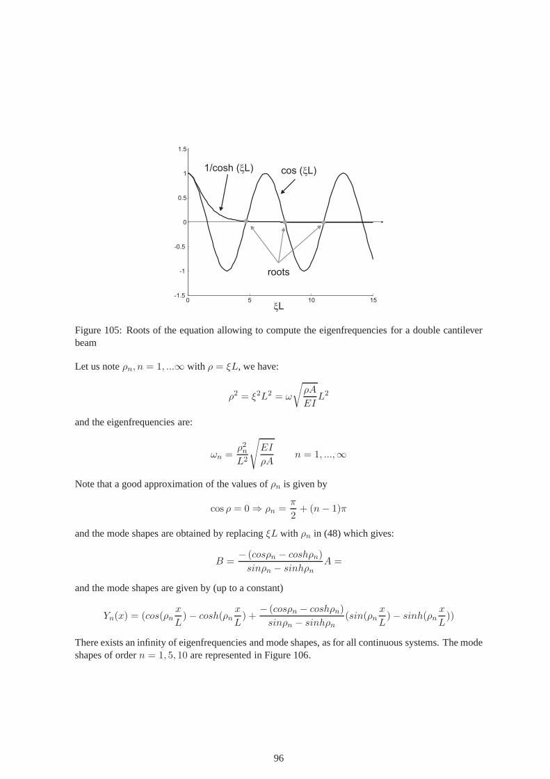
0 5 10 15-1.5

-1

-0.5

0

0.5

1

1.5

cos ( L)x1/cosh ( L)x

xL

roots

Figure 105: Roots of the equation allowing to compute the eigenfrequencies for a double cantileverbeam

Let us noteρn, n = 1, ...∞ with ρ = ξL, we have:

ρ2 = ξ2L2 = ω

√

ρA

EIL2

and the eigenfrequencies are:

ωn =ρ2nL2

√

EI

ρAn = 1, ...,∞

Note that a good approximation of the values ofρn is given by

cos ρ = 0 ⇒ ρn =π

2+ (n− 1)π

and the mode shapes are obtained by replacingξL with ρn in (48) which gives:

B =− (cosρn − coshρn)

sinρn − sinhρnA =

and the mode shapes are given by (up to a constant)

Yn(x) = (cos(ρnx

L)− cosh(ρn

x

L) +

− (cosρn − coshρn)

sinρn − sinhρn(sin(ρn

x

L)− sinh(ρn

x

L))

There exists an infinity of eigenfrequencies and mode shapes, as for all continuous systems. The modeshapes of ordern = 1, 5, 10 are represented in Figure 106.

96

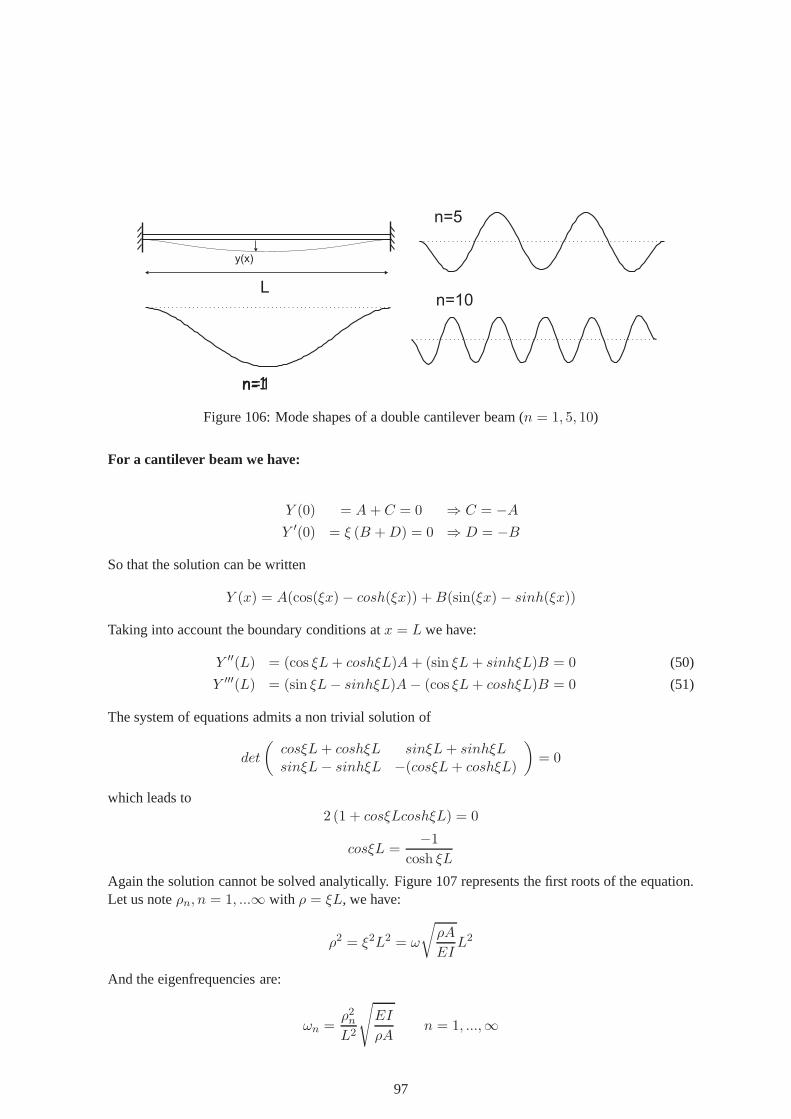
y(x)

L

n=1n=1

n=5

n=10

Figure 106: Mode shapes of a double cantilever beam (n = 1, 5, 10)

For a cantilever beam we have:

Y (0) = A+ C = 0 ⇒ C = −AY ′(0) = ξ (B +D) = 0 ⇒ D = −B

So that the solution can be written

Y (x) = A(cos(ξx)− cosh(ξx)) +B(sin(ξx)− sinh(ξx))

Taking into account the boundary conditions atx = L we have:

Y ′′(L) = (cos ξL+ coshξL)A+ (sin ξL+ sinhξL)B = 0 (50)

Y ′′′(L) = (sin ξL− sinhξL)A− (cos ξL+ coshξL)B = 0 (51)

The system of equations admits a non trivial solution of

det

(

cosξL+ coshξL sinξL+ sinhξLsinξL− sinhξL −(cosξL+ coshξL)

)

= 0

which leads to2 (1 + cosξLcoshξL) = 0

cosξL =−1

cosh ξL

Again the solution cannot be solved analytically. Figure 107 represents the first roots of the equation.Let us noteρn, n = 1, ...∞ with ρ = ξL, we have:

ρ2 = ξ2L2 = ω

√

ρA

EIL2

And the eigenfrequencies are:

ωn =ρ2nL2

√

EI

ρAn = 1, ...,∞

97

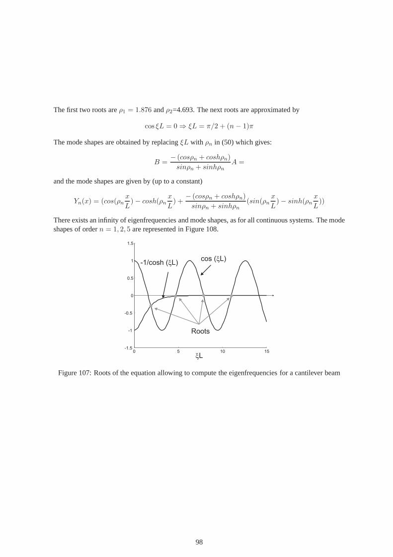
The first two roots areρ1 = 1.876 andρ2=4.693. The next roots are approximated by

cos ξL = 0 ⇒ ξL = π/2 + (n − 1)π

The mode shapes are obtained by replacingξL with ρn in (50) which gives:

B =− (cosρn + coshρn)

sinρn + sinhρnA =

and the mode shapes are given by (up to a constant)

Yn(x) = (cos(ρnx

L)− cosh(ρn

x

L) +

− (cosρn + coshρn)

sinρn + sinhρn(sin(ρn

x

L)− sinh(ρn

x

L))

There exists an infinity of eigenfrequencies and mode shapes, as for all continuous systems. The modeshapes of ordern = 1, 2, 5 are represented in Figure 108.

0 5 10 15-1.5

-1

-0.5

0

0.5

1

1.5

cos ( L)x-1/cosh ( L)x

xL

Roots

Figure 107: Roots of the equation allowing to compute the eigenfrequencies for a cantilever beam

98

n=1

n=2

n=5

Figure 108: Mode shapes of a cantilever beam (n = 1, 2, 5)

6.1.10 Beam in bending: orthogonality conditions

For beams in bending, the orthogonality conditions are given by:∫ L

0ρAYi Yj dx = δijµi

∫ L

0EIY ′′

i Y′′j dx = δijµiω

2i

Proof: Let us consider two different mode shapesYi andYj whereωi 6= ωj:

EIY IVi + ρAω2

i Yi = 0 (52)

EIY IVj + ρAω2

jYj = 0 (53)

we multiply (52) byYj and integrate from 0 toL, and multiply (53) byYi and integrate from 0 toL.

∫ L

0

(

EIY IVi + ρAω2

i Yi)

Yj dx = 0 (54)

∫ L

0

(

EIY IVj + ρAω2

jYj)

Yi dx = 0 (55)

Integrating twice by parts, we have∫ L

0EI Y IV

i Yj dx =[

EI Y IIIi Yj

]L

0−∫ L

0EI Y III

i Y ′j dx+

=[

EI Y IIIi Yj

]L

0−[

EI Y ′′i Y

′j

]L

0+

∫ L

0EI Y ′′

i Y′′j dx

The term[

EI Y IIIi Yj

]L

0

99

is always equal to zero because we either haveY = 0 or T = 0 (which leads toT = −EIY III = 0)at the boundaries of the beam, and the term

[

EI Y ′′i Y

′j

]L

0

is also always equal to zero because we either haveY ′ = 0 orM = 0 at the boundaries of the beam(which leads to−EIY ′′ = 0). Finally, we obtain:

∫ L

0EI Y IV

i Yj dx =

∫ L

0EI Y ′′

j Y′′i dx

and in the same way∫ L

0EI Y IV

j Yi dx =

∫ L

0EI Y ′′

i Y′′j dx

Therefore we have:∫ L

0EI Y ′′

j Y′′i + ρAω2

i YjYidx = 0 (56)

∫ L

0EI Y ′′

i Y′′j + ρAω2

jYiYjdx = 0 (57)

Substracting (57) from (56), we have:

∫ L

0ρA(ω2

i − ω2j )Yi Yj dx = 0 i 6= j (58)

so that∫ L

0ρAYi Yj dx = 0 i 6= j (59)

and defining

µi =

∫ L

0ρAY 2

i dx (60)

(59) and (60) give the second orthogonality condition.We can rewrite (56):

∫ L

0EI Y ′′

j Y′′i = −ρAω2

i YjYidx

and taking into account (59) and (60), we have:

∫ L

0EI Y ′′

i Y′′j dx = 0 i 6= j

∫ L

0EI (Y ′′

i )2 dx = ω2

i µi

which is the first orthogonality condition.

100

6.1.11 Beam in bending: projection in the modal basis

Starting from the equation of motion

EI∂4y(x, t)

∂x4+ ρA

∂2y(x, t)

∂t2= p(x, t)

we assume that the solution can be written as a function of themode shapes

y(x, t) =

∞∑

i=1

Yi(x)zi(t)

Plugging into the equation of motion, we have

EI∞∑

i=1

Y IVi zi + ρA

∞∑

i=1

Yizi = p(x, t)

We multiply byYj and integrate from 0 toL:

∫ L

0

(

EI

∞∑

i=1

Y IVi zi

)

Yj dx+

∫ L

0

(

ρA

∞∑

i=1

Yizi

)

Yj dx =

∫ L

0p(x, t)Yj dx

and rearranging

∫ L

0

(

EI

∞∑

i=1

Y IVi Yj

)

zi dx+

∫ L

0

(

ρA

∞∑

i=1

YiYj

)

zi dx =

∫ L

0p(x, t)Yj dx

the orthogonality conditions are then used to obtain

µizi + µiω2i zi = Fi

Fi =

∫ L

0p(x, t)Yi dx

As in the case of the bar in traction, the equation of motion istransformed into an infinite number ofequations of motions of a single dof. As discussed earlier, atruncation can be performed based on thefrequency band of interest for the computation. Below is a link to a video showing the first modes ofa cantilever beam.

Cantilever beam modes : http://www.youtube.com/watch?v=uBZqa851uvw

6.2 Complex structures

In many cases, the complexity of a structure does not allow one to use a beam or bar model in orderto get an accurate model. There exist also solution for rectangular plates, but this will not be treatedin this course. For more general cases, it is necessary to build an approximation by using numericalmodels, the most widely used being the finite element method.In the finite element method, thestructure is divided in elements and contains nodes. For a general 3D model, there are three unknownsfor each node: the displacement in the 3 directions. The displacement field is therefore given by:

101

u(x, y, z)v(x, y, z)w(x, y, z)

=

n∑

i=1

uiφi(x, y, z)

n∑

i=1

viφi(x, y, z)

n∑

i=1

wiφi(x, y, z)

whereu, v, w are the displacement in thex, y andz direction,n is the number of nodes in the model,φi(x, y, z) are the shape functions andui, vi, wi are the nodal displacements of nodei. An exampleof a finite element model of a bridge is presented in Figure 109.

Figure 109: Finite element model of the Pine Creek bridge lenticular truss bridge(http://fynitesolutions.com)

Another example is given in Figure 110. The study concerns the interaction of vehicles withthe bridge. Once the finite element has been built, it is possible to obtain the stiffness and the massmatrices. The size of these matrices depends on the number ofdofs of the structure modeled. For astructure modeled with 3D elements, the number of unknowns is 3n wheren is the number of nodes.The matricesK andM are therefore 3n x 3nmatrices. The undamped equations of motion are writtenin a matrix form:

Mq +Kq = F

where

q =

u1v1w1

u2...wn

is the vector of nodal unknowns. As this expression is identical to (27), the tools described in sec-tion 5.1 can be used to solve the system of equations. Based ontheK andM matrices, the modeshapes and eigenfrequencies can be computed numerically. Afew mode shapes of the bridge arerepresented on Figure 111. From that point, the same strategy as described for mdof systems can befollowed to reduce the system of equations by projecting it in the modal basis. In general, the numberof dofs in the model is not linked to the necessary accuracy, but rather to the necessity to comply withthe complex geometry. For a bridge excited by wind and traffic, generally, only a few modes (up to

102

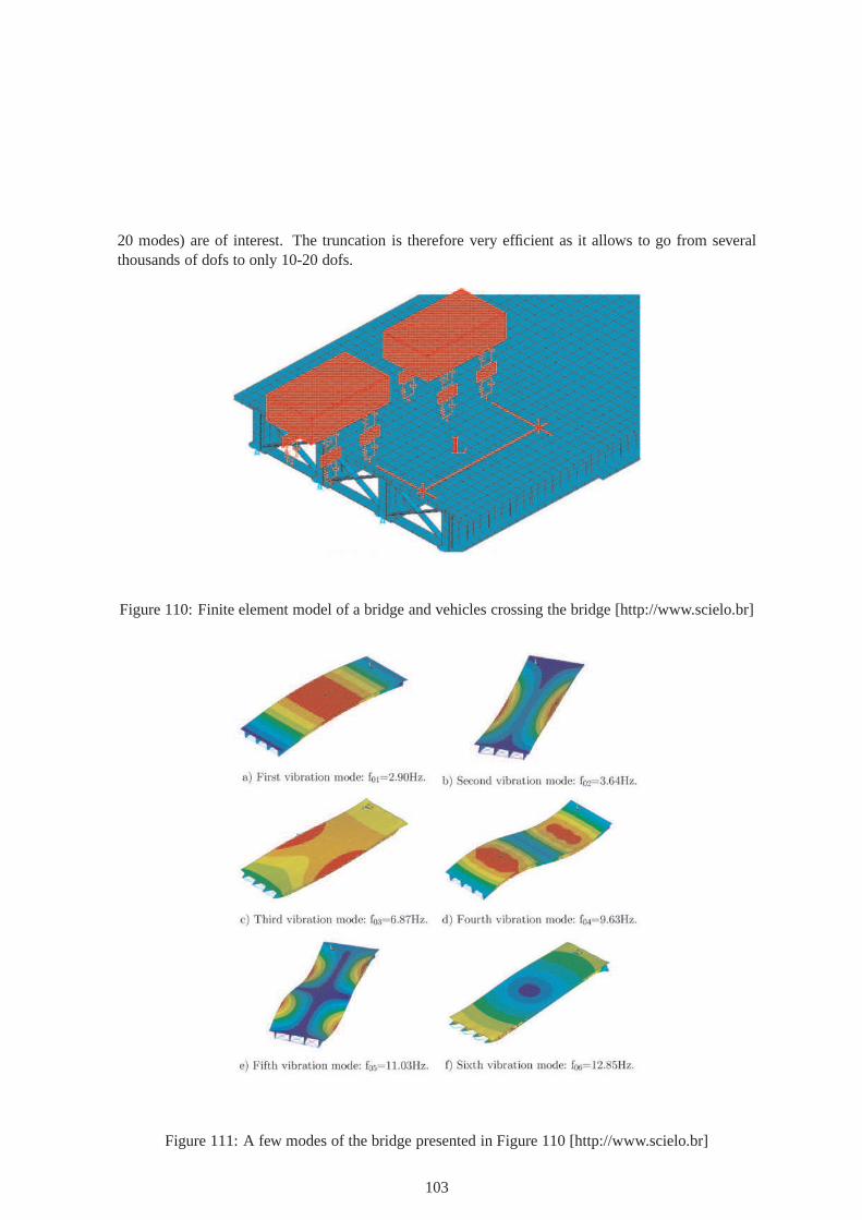
20 modes) are of interest. The truncation is therefore very efficient as it allows to go from severalthousands of dofs to only 10-20 dofs.

Figure 110: Finite element model of a bridge and vehicles crossing the bridge [http://www.scielo.br]

Figure 111: A few modes of the bridge presented in Figure 110 [http://www.scielo.br]

103

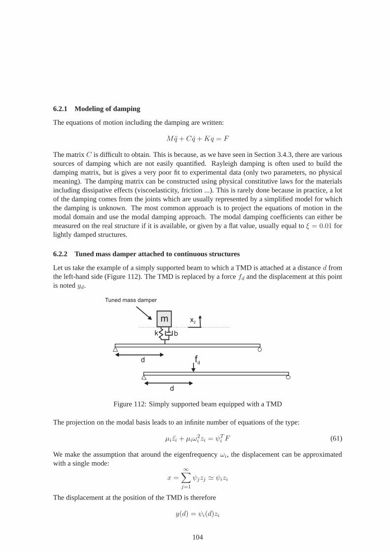
6.2.1 Modeling of damping

The equations of motion including the damping are written:

Mq + Cq +Kq = F

The matrixC is difficult to obtain. This is because, as we have seen in Section 3.4.3, there are varioussources of damping which are not easily quantified. Rayleighdamping is often used to build thedamping matrix, but is gives a very poor fit to experimental data (only two parameters, no physicalmeaning). The damping matrix can be constructed using physical constitutive laws for the materialsincluding dissipative effects (viscoelasticity, friction ...). This is rarely done because in practice, a lotof the damping comes from the joints which are usually represented by a simplified model for whichthe damping is unknown. The most common approach is to project the equations of motion in themodal domain and use the modal damping approach. The modal damping coefficients can either bemeasured on the real structure if it is available, or given bya flat value, usually equal toξ = 0.01 forlightly damped structures.

6.2.2 Tuned mass damper attached to continuous structures

Let us take the example of a simply supported beam to which a TMD is attached at a distanced fromthe left-hand side (Figure 112). The TMD is replaced by a force fd and the displacement at this pointis notedyd.

k

m x2

Tuned mass damper

b

fdd

d

Figure 112: Simply supported beam equipped with a TMD

The projection on the modal basis leads to an infinite number of equations of the type:

µizi + µiω2i zi = ψT

i F (61)

We make the assumption that around the eigenfrequencyωi, the displacement can be approximatedwith a single mode:

x =

∞∑

j=1

ψjzj ≃ ψizi

The displacement at the position of the TMD is therefore

y(d) = ψi(d)zi

104

and we can write

zi =y(d)

ψi(d)

Replacing in (61) and noting thatψTi F = ψi(d)fd, we obtain:

µiψ2i (d)

y(d) +µiω

2i

ψ2i (d)

y(d) = fd

which can be writtenMy(d) +Ky(d) = fd

if we define

M =µi

ψ2i (d)

K =µiω

2i

ψ2i (d)

The equation of motion has been reduced to a single dof (assuming that the displacement can beapproximated by a single mode), and the formulae developed in Section 5.3 can be used. Figure 113shows the example of the displacement in the middle of the beam excited by a force at the samelocation, with and without the TMD. The TMD is efficient to damp the first mode. Note that it iseffective only in a narrow frequency band around the frequency to which it has been tuned.

101

102

103

10-10

10-8

10-6

10-4

10-2

Frequency (Hz)

X/F

(dB

)1

Without TMD

With TMDtuned on mode 1

Figure 113: Displacement in the middle of the beam due to a force at the same location. Effect of theTMD

The following movie illustrates the efficiency of a TMD to damp the first mode shape of a can-tilever beam.

Beam with tuned mass damper: http://www.youtube.com/watch?v=fuCdZLQOrAw

105