dynamics and control of formation flying satellites in earth … · 2004-09-08 · dynamics and...
TRANSCRIPT
Alfriend/Barcelona 1
Dynamics and Control ofFormation Flying Satellites
In Earth OrbitLecture 2Terry Alfriend
Texas A&M University
Alfriend/Barcelona 2
Outline
• Example of the Error Analysis of a LEO satellite• Navigation Error Effect• Constellation Control• Impulsive and Continuous Control of Orbital
Elements
Lecture 2- Control Concepts and Navigation Error Effect

Alfriend/Barcelona 3
Error Analysis of a LEO satellite
Ref: Alfriend, K.T. and Lovell, T.A.,“Error Analysis of SatelliteFormations In Near Circular Low Earth Orbits,” Paper No. AAS03-651,2003 AAS/AIAA Astrodynamics Conference, Big Sky, MT, Aug. 2003.

Alfriend/Barcelona 4
Outline
• Background• Maneuver Strategy• Analytical Insights• Error Analysis• Conclusions
Alfriend/Barcelona 5
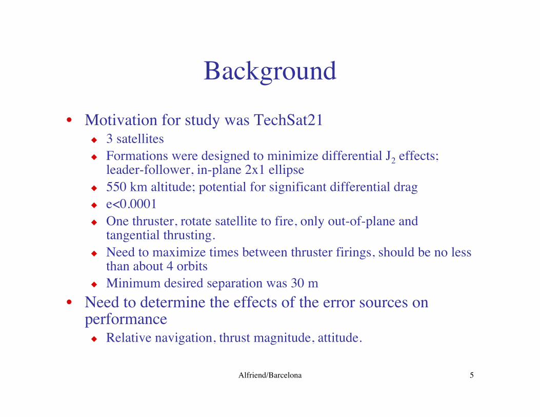
Background• Motivation for study was TechSat21
u 3 satellitesu Formations were designed to minimize differential J2 effects;
leader-follower, in-plane 2x1 ellipseu 550 km altitude; potential for significant differential dragu e<0.0001u One thruster, rotate satellite to fire, only out-of-plane and
tangential thrusting.u Need to maximize times between thruster firings, should be no less
than about 4 orbitsu Minimum desired separation was 30 m
• Need to determine the effects of the error sources onperformance
u Relative navigation, thrust magnitude, attitude.
Alfriend/Barcelona 6
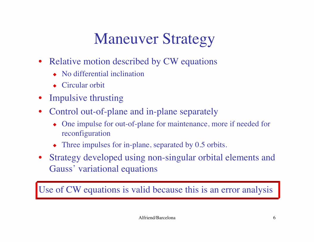
Maneuver Strategy• Relative motion described by CW equations
u No differential inclinationu Circular orbit
• Impulsive thrusting• Control out-of-plane and in-plane separately
u One impulse for out-of-plane for maintenance, more if needed forreconfiguration
u Three impulses for in-plane, separated by 0.5 orbits.• Strategy developed using non-singular orbital elements and
Gauss’ variational equations
Use of CW equations is valid because this is an error analysis

Alfriend/Barcelona 7
Drag/ Cross Section Area Model
Satellite is thin parallelepiped that tracks the sun and slowlyrotates at orbit rate. The orientation is such that the velocityvector is nearly perpendicular to A2. Model deteriorates as sunapproaches orbit plane, but this is where differential drag effectis minimum.
A3
bSun
Orbit Normal (Z)
A2
A1
A = A1
re
u◊ re
y+ A
2
re
v◊ re
y+ A
3
re
w◊ re
y
A = 0.5A1
1 - cos b( ) sin2q + 0.5A2
1 + cos b( ) - 1 - cos b( )cos2qÈÎ ˘̊ + A3
sin b cosq
A = 0.5A1
1 - cos b( ) 4
2psin 2qdq
0
p / 2
Ú + 0.5A2
1
2p1 + cos b( ) + 1 - cos b( )cos2qÈÎ ˘̊ dq
0
2p
Ú
+ A3sin b 2
2pcosqdq
- p / 2
p / 2
Ú
A =A
1
p1 - cos b( ) + 0.5A
21 + cos b( ) +
A3
psin b
Alfriend/Barcelona 8
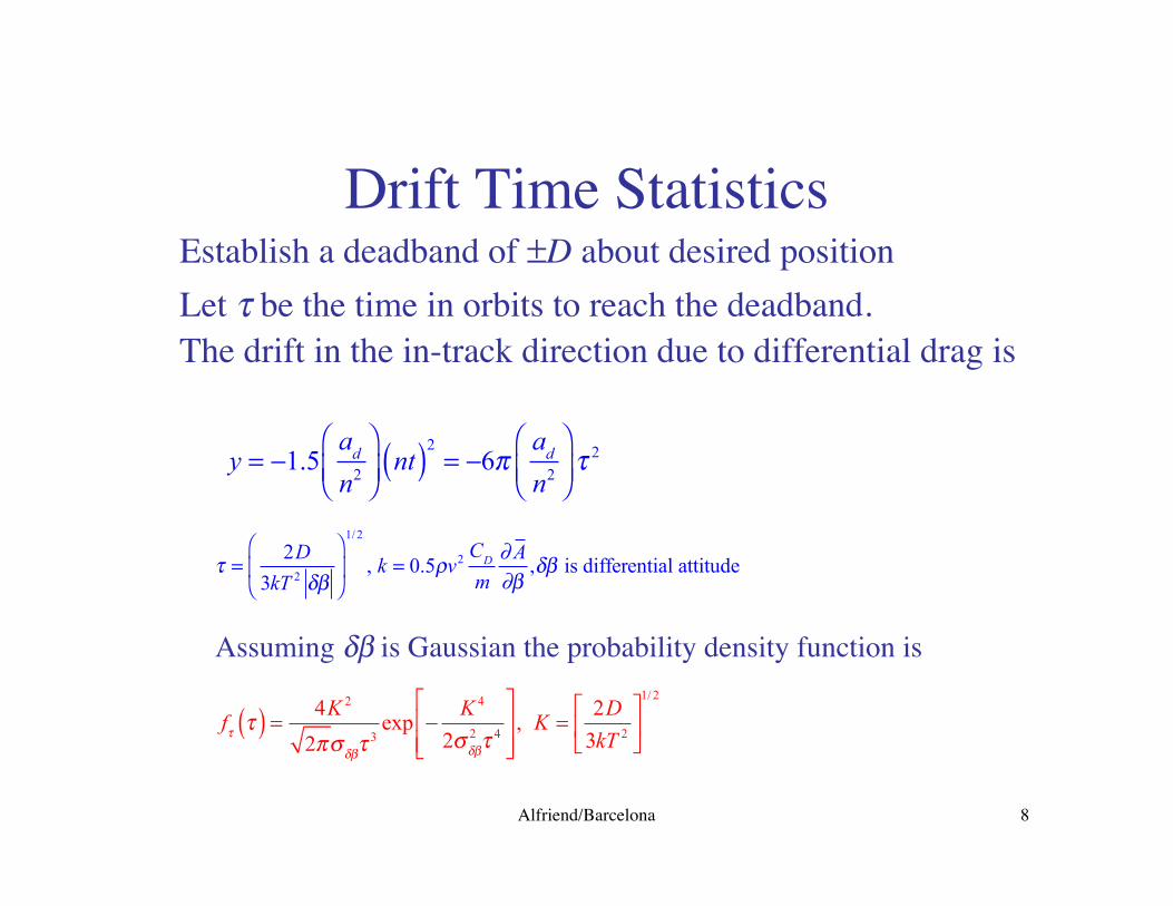
Drift Time StatisticsEstablish a deadband of ±D about desired positionLet t be the time in orbits to reach the deadband.The drift in the in-track direction due to differential drag is
y = -1.5
ad
n2
Ê
ËÁˆ
¯̃nt( )2
= -6pa
d
n2
Ê
ËÁˆ
¯̃t 2
t =2D
3kT 2 db
Ê
ËÁ
ˆ
¯˜
1/ 2
, k = 0.5rv2 CD
m
∂ A
∂b,db is differential attitude
ft t( ) =4K 2
2p s dbt 3exp -
K 4
2s db2 t 4
È
ÎÍÍ
˘
˚˙˙, K =
2D
3kT 2
È
ÎÍ
˘
˚˙
1/ 2
Assuming db is Gaussian the probability density function is
Alfriend/Barcelona 9
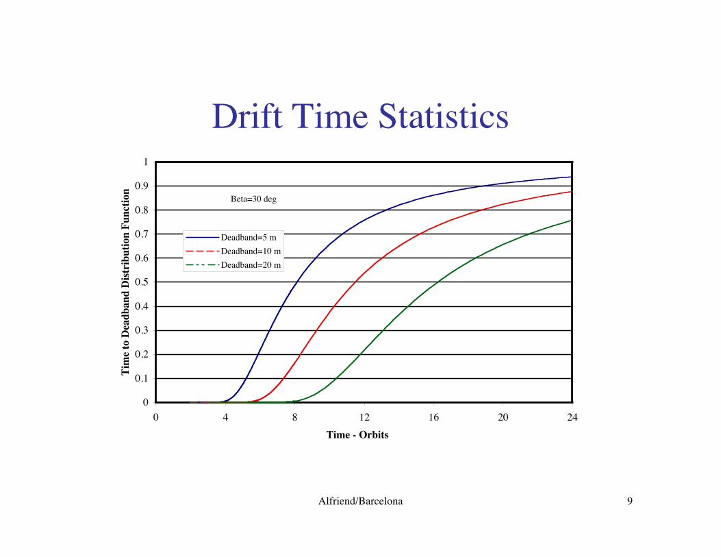
Drift Time Statistics
0
0.1
0.2
0.3
0.4
0.5
0.6
0.7
0.8
0.9
1
0 4 8 12 16 20 24Time - Orbits .
Tim
e to
Dea
dban
d D
istri
butio
n Fu
nctio
n
Deadband=5 mDeadband=10 mDeadband=20 m
Beta=30 deg
Alfriend/Barcelona 10
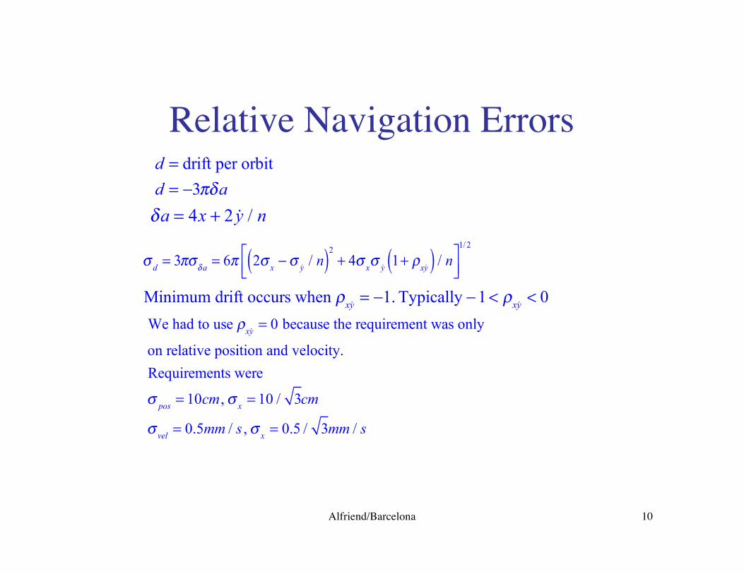
Relative Navigation Errors
d a = 4x + 2 &y / n
d = drift per orbit
d = -3pd a
s
d= 3ps d a
= 6p 2sx
- s &y / n( )2
+ 4sx
s &y 1 + rx&y( ) / nÈ
Î͢˚̇
1/ 2
Minimum drift occurs when r
x&y = -1. Typically - 1 < rx&y < 0
We had to use rx&y = 0 because the requirement was only
on relative position and velocity.
Requirements were
spos
= 10cm, sx
= 10 / 3cm
svel
= 0.5mm / s , sx
= 0.5 / 3mm / s

Alfriend/Barcelona 11
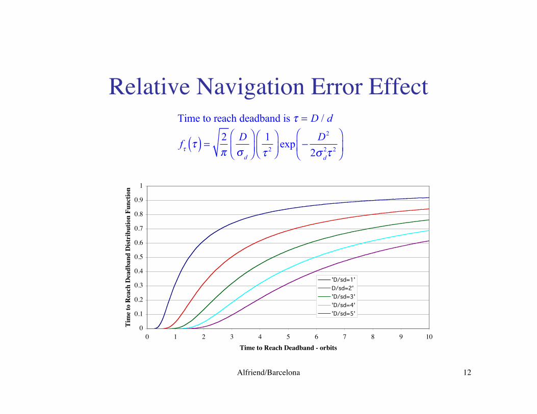
Relative Navigation Error Effect
0
0.8
1.6
2.4
3.2
4
4.8
5.6
6.4
7.2
0 0.1 0.2 0.3 0.4Relative Rate Standard Deviation - mm/s
Dri
ft R
ate S
tand
ard
Dev
iatio
n - m
/orb
it
'sig x=0 cm''sig x=2 cm''sig x=4 cm''sig x=6 cm''sig x=8 cm'Requirement
Relative velocity error is driver.
Alfriend/Barcelona 12
Relative Navigation Error Effect
0
0.1
0.2
0.3
0.4
0.5
0.6
0.7
0.8
0.9
1
0 1 2 3 4 5 6 7 8 9 10Time to Reach Deadband - orbits
Tim
e to
Rea
ch D
eadb
and
Dist
ribu
tion
Func
tion
'D/sd=1'D/sd=2''D/sd=3''D/sd=4''D/sd=5'
Time to reach deadband is t = D / d
ft t( ) =2
pD
sd
Ê
ËÁˆ
¯̃1
t 2
ÊËÁ
ˆ¯̃
exp -D2
2sd2t 2
Ê
ËÁ
ˆ
¯˜
Alfriend/Barcelona 13
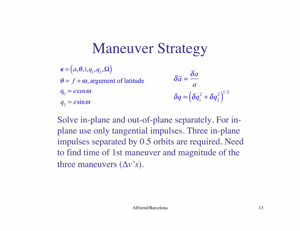
Maneuver Strategy
e = a,q ,i,q1,q
2,W( )
q = f + w , argument of latitude
q1
= ecoswq
2= esinw
d a =d a
a
dq = dq12 + dq
22( )1/ 2
Solve in-plane and out-of-plane separately. For in-plane use only tangential impulses. Three in-planeimpulses separated by 0.5 orbits are required. Needto find time of 1st maneuver and magnitude of thethree maneuvers (Dv’s).

Alfriend/Barcelona 14
Gauss’ Variational Equations
Dq1
= 2Dv
t
vc
cosq
Dq2
= 2Dv
t
vc
sinq
Da =2
nDv
t
Di =Dv
n
vc
cosq
DW =Dv
n
vcsin i
sinq
Dq = -cot isinq
vc
Dvn
Da = -2
nDv
1+ Dv
2+ Dv
3( )Dq
1= -
2
naDv
1- Dv
2+ Dv
3( )cosq1
Dq2
= -2
naDv
1- Dv
2+ Dv
3( )sinq1
tanq
1=
Dq2
Dq1
Dvn
= Di2 + DWsin i( )2ÈÎÍ
˘˚̇
1/ 2
tanqoop
=DWsin i
Di
D denotes the change in the element.
Alfriend/Barcelona 15
Strategy
• Separate into out-of-plane and in-plane.• Out-of-plane is one maneuver.• In-plane is three maneuvers, separated by 0.5 orbit.
u Time of first maneuver determined by required elementchanges.
u 4 unknowns, four equationsu Tangential thrust only
Alfriend/Barcelona 16
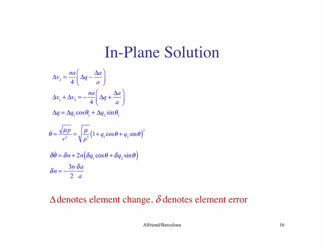
In-Plane Solution
Dv2
=na
4Dq -
Da
a
ÊËÁ
ˆ¯̃
Dv1
+ Dv3
= -na
4Dq +
Da
a
ÊËÁ
ˆ¯̃
Dq = Dq1cosq
1+ Dq
2sinq
1
&q =m p
r 2=
mp3
1 + q1cosq + q
2sinq( )2
�
d ˙ q = dn + 2n dq1 cos q + dq2 sinq( )dn = - 3n
2daa
d &q = d n + 2n dq1cosq + dq
2sinq( )
d n = -3n
2
d a
a
D denotes element change, d denotes element error
Alfriend/Barcelona 17
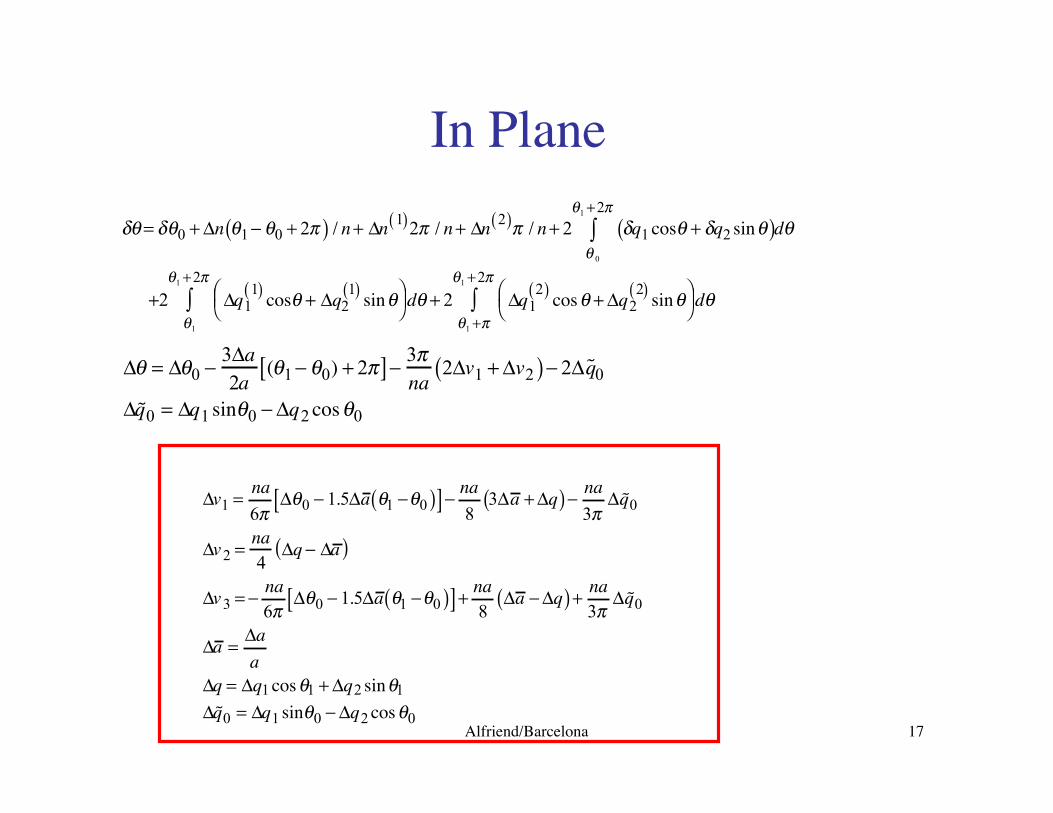
In Plane
�
dq = dq0 + Dn q1 - q0 + 2p( ) / n + Dn 1( ) 2p / n + Dn 2( )p / n + 2 dq1 cosq + dq2 sin q( )dqq 0
q1 + 2p
Ú
+2 Dq11( ) cosq + Dq2
1( ) sin qÊ Ë Á ˆ
¯ ˜ dqq1
q1 + 2p
Ú + 2 Dq12( ) cos q + Dq2
2( ) sin qÊ Ë Á ˆ
¯ ˜ dqq1 +p
q1 + 2p
Ú
�
Dq = Dq0 - 3Da2a
(q1 - q0) + 2p[ ] - 3pna
2Dv1 + Dv2( ) - 2D ˜ q 0
D ˜ q 0 = Dq1 sinq0 - Dq2 cos q0
�
Dv1 = na6p
Dq0 - 1.5Da q1 - q0( )[ ] - na8
3Da + Dq( ) - na3p
D ˜ q 0
Dv2 = na4
Dq - Da ( )
Dv3 = - na6p
Dq0 - 1.5Da q1 - q0( )[ ] + na8
Da - Dq( ) + na3p
D ˜ q 0
Da = Daa
Dq = Dq1 cos q1 + Dq2 sin q1
D ˜ q 0 = Dq1 sinq0 - Dq2 cos q0

Alfriend/Barcelona 18
Error Sources
Table 1 Baseline Error Sources
Error Source Pointing(deg)
Position(m)
Velocity(mm/s)
Thrust(%)
Value - 1s 1/3 0.1/31/2 0.5/31/2 5
Table 2 Baseline System Parameter Values
Parameter Deadband(m)
Altitude(km)
Density(kg/m3)
A1(m2)
A2(m2)
A3(m2)
b(deg)
mass(kg)
Value 5, 10,
15,20
550 3.183 x10⁻¹³ 0.575 0.82 12.984 30 170

Alfriend/Barcelona 19
Approach
• All error sources selected from random number generator withspecified standard deviation
• Start in desired formation, generate differential drag from attitudeerror.
• When 75% of deadband reached initiate maneuver decision.• To compute desired Dv’s corrupt exact relative state with navigation
system errors. Actual Dv is corrupted in magnitude by thrustmagnitude error source and direction by attitude error. New attitudeerror generated after each maneuver.
• Once maneuver initiated not recalculated based on new estimated state.Option exists to recalculate last Dv to force estimated drift to zero.Results show not effective because of navigation error.
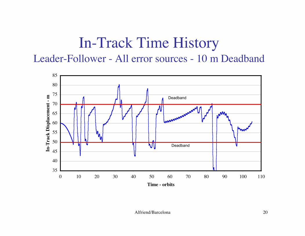
Alfriend/Barcelona 20
In-Track Time HistoryLeader-Follower - All error sources - 10 m Deadband
35
40
45
50
55
60
65
70
75
80
85
0 10 20 30 40 50 60 70 80 90 100 110Time - orbits
In-T
rack
Disp
lace
men
t - m Deadband
Deadband
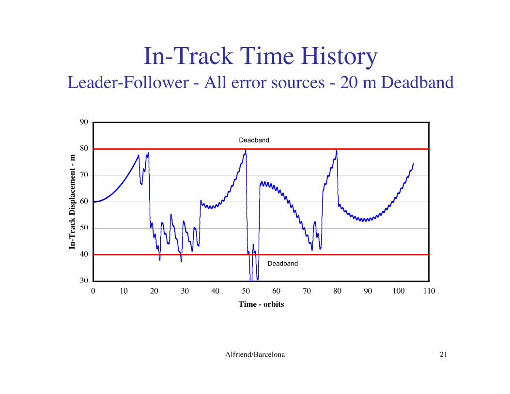
Alfriend/Barcelona 21
In-Track Time HistoryLeader-Follower - All error sources - 20 m Deadband
30
40
50
60
70
80
90
0 10 20 30 40 50 60 70 80 90 100 110Time - orbits
In-T
rack
Disp
lace
men
t - m
Deadband
Deadband
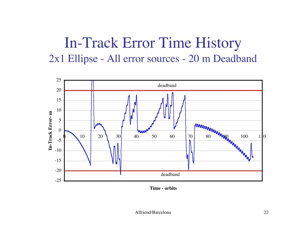
Alfriend/Barcelona 22
In-Track Error Time History2x1 Ellipse - All error sources - 20 m Deadband
-25
-20
-15
-10
-5
0
5
10
15
20
25
0 10 20 30 40 50 60 70 80 90 100 110
Time - orbits
In-T
rack
Err
or- m
deadband
deadband
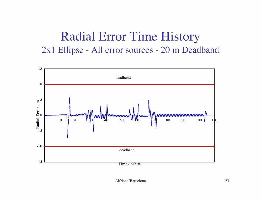
Alfriend/Barcelona 23
Radial Error Time History2x1 Ellipse - All error sources - 20 m Deadband
-15
-10
-5
0
5
10
15
0 10 20 30 40 50 60 70 80 90 100 110
Time - orbits
Rad
ial E
rror
- m
deadband
deadband
Alfriend/Barcelona 24
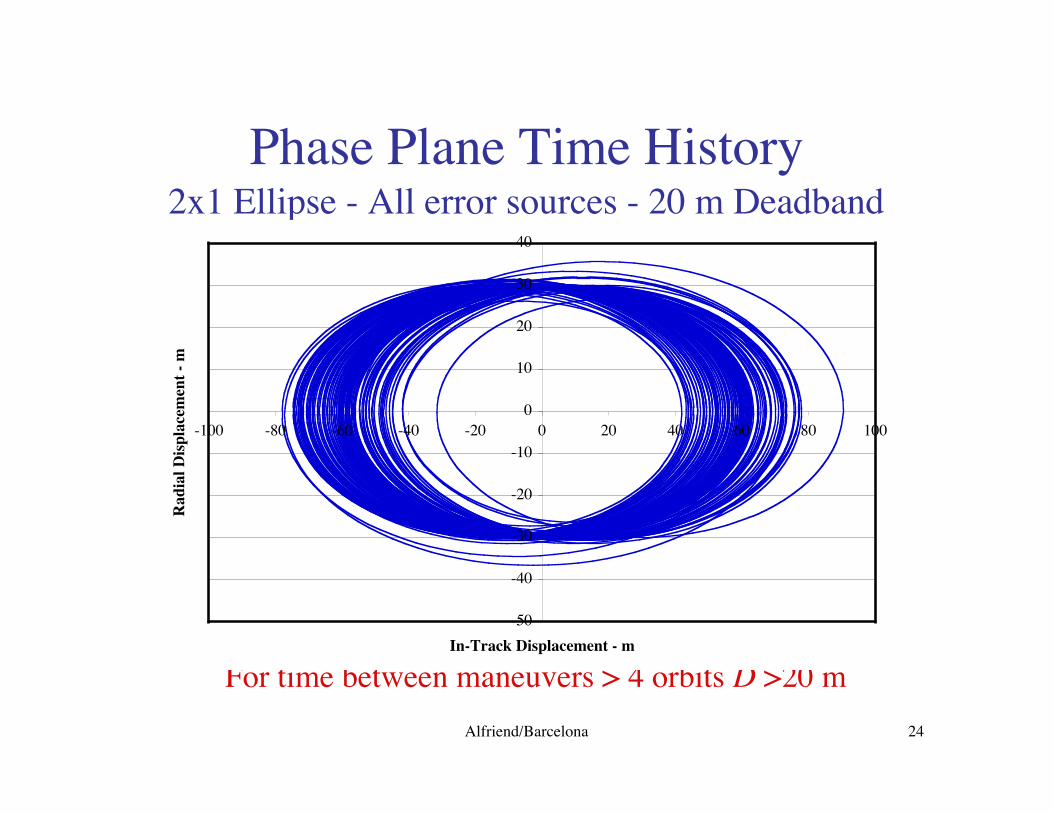
Phase Plane Time History2x1 Ellipse - All error sources - 20 m Deadband
For time between maneuvers > 4 orbits D >20 m
-50
-40
-30
-20
-10
0
10
20
30
40
-100 -80 -60 -40 -20 0 20 40 60 80 100
In-Track Displacement - m
Rad
ial D
ispla
cem
ent -
m
Alfriend/Barcelona 25
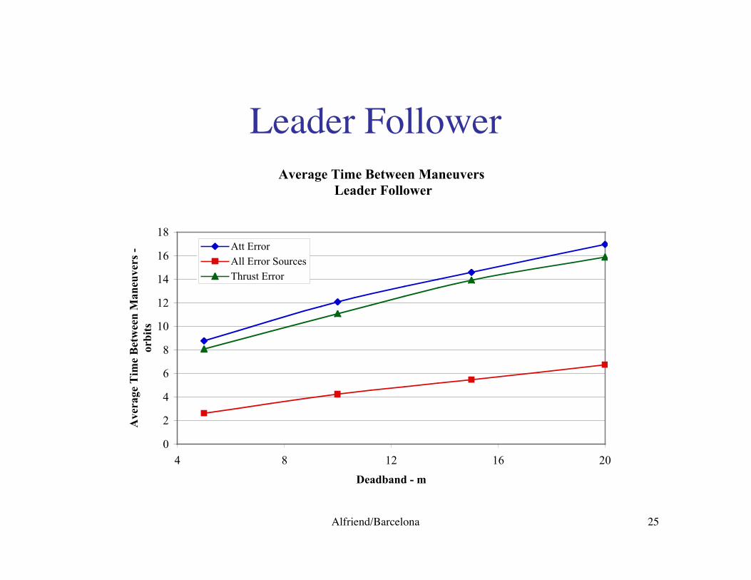
Leader FollowerAverage Time Between Maneuvers
Leader Follower
0
2
4
6
8
10
12
14
16
18
4 8 12 16 20
Deadband - m
Ave
rage
Tim
e B
etw
een
Man
euve
rs -
or
bits
Att ErrorAll Error SourcesThrust Error
Alfriend/Barcelona 26
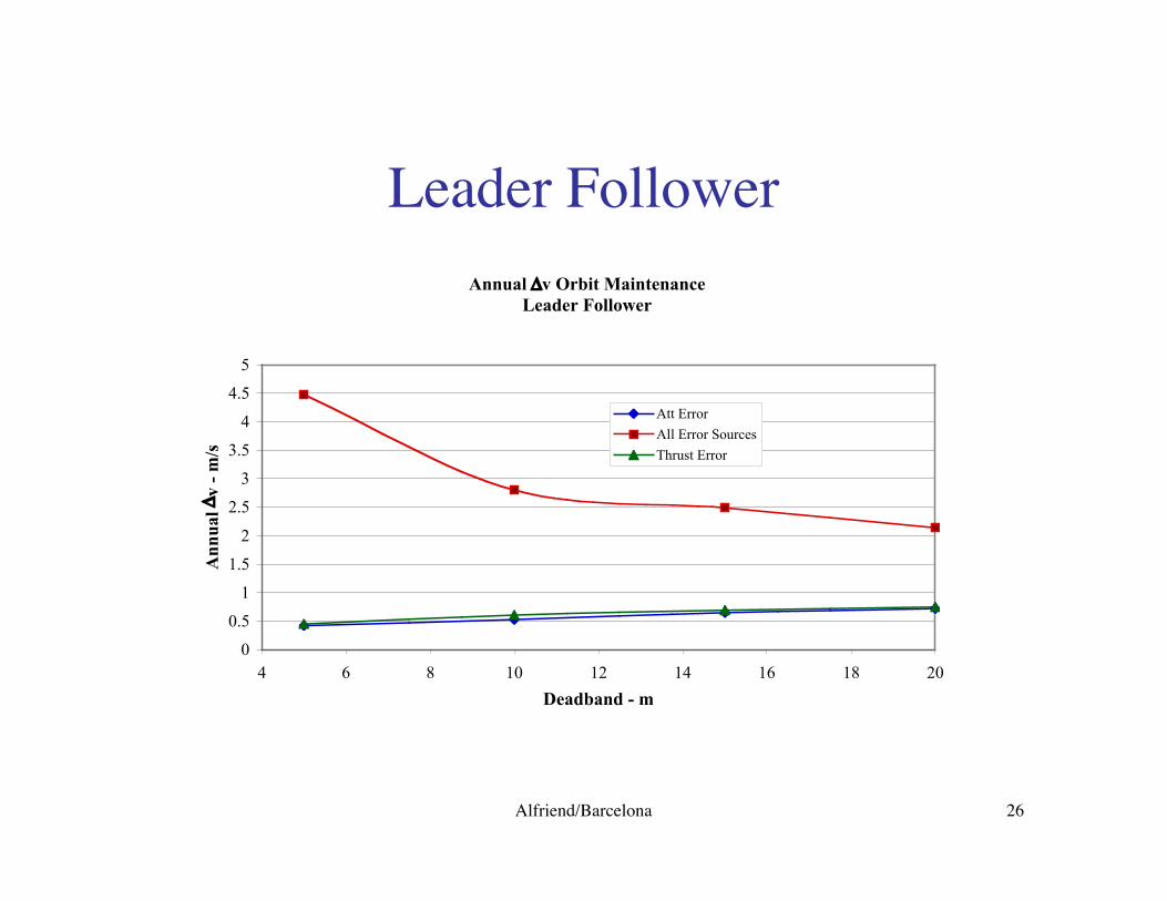
Leader FollowerAnnual Dv Orbit Maintenance
Leader Follower
0
0.5
1
1.5
2
2.5
3
3.5
4
4.5
5
4 6 8 10 12 14 16 18 20
Deadband - m
Ann
ual D
v -
m/s
Att Error
All Error Sources
Thrust Error

Alfriend/Barcelona 27
LF-CIPE Comparison
Average Time Between Maneuvers LF-CIPE Comparison
0
1
2
3
4
5
6
7
8
4 8 12 16 20
Deadband - m
Ave
. Tim
e B
etw
een
Man
euve
rs -
orbi
ts
LFCIPE
All Error sources
Alfriend/Barcelona 28
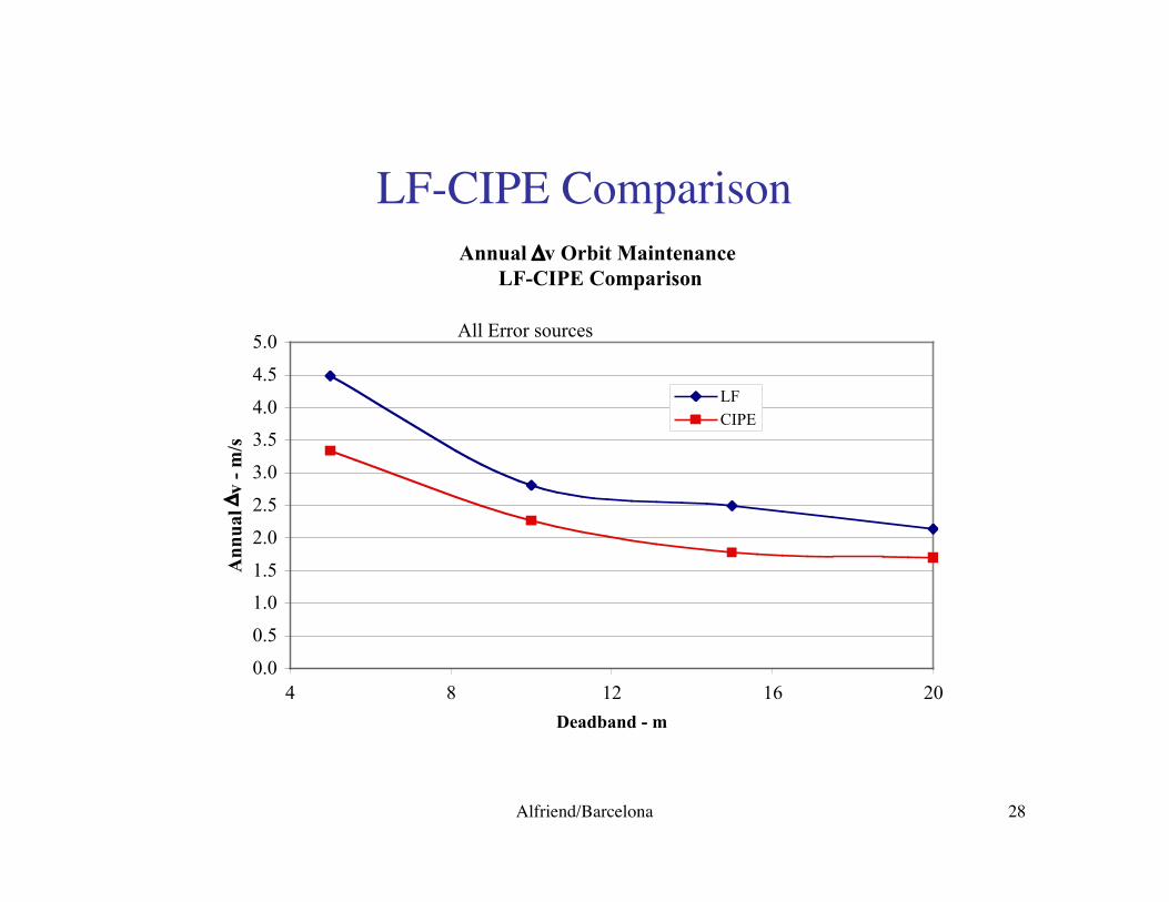
LF-CIPE ComparisonAnnual Dv Orbit Maintenance
LF-CIPE Comparison
0.0
0.5
1.0
1.5
2.0
2.5
3.0
3.5
4.0
4.5
5.0
4 8 12 16 20
Deadband - m
Ann
ual D
v -
m/s
LFCIPE
All Error sources

Alfriend/Barcelona 29
Distribution Function
0
0.1
0.2
0.3
0.4
0.5
0.6
0.7
0.8
0.9
1
0 5 10 15 20 25 30 35 40Time Between Maneuvers - orbits
Dist
ribu
tion
Func
tion
TheoryAll ErrorsNav Errors
Alfriend/Barcelona 30
Conclusions• The minimum acceptable deadband is about 20 meters. Even with a
20-meter deadband the deadband may be exceeded on occasion.• To guarantee that the motion stay within the 20-meter deadband will
require a new method for formation maintenance that responds faster.This will increase the fuel consumption.
• The relative navigation errors, particularly the relative velocity error,are the driver for the minimum acceptable deadband.
• Rel nav requirements should include a requirement on cross-correlation and on drift rate.
• The fuel, or Dv, required for orbit maintenance is minimal.• The 5% 1s thrust error has very little effect on the average time
between maneuvers or the annual fuel requirement.
Alfriend/Barcelona 31
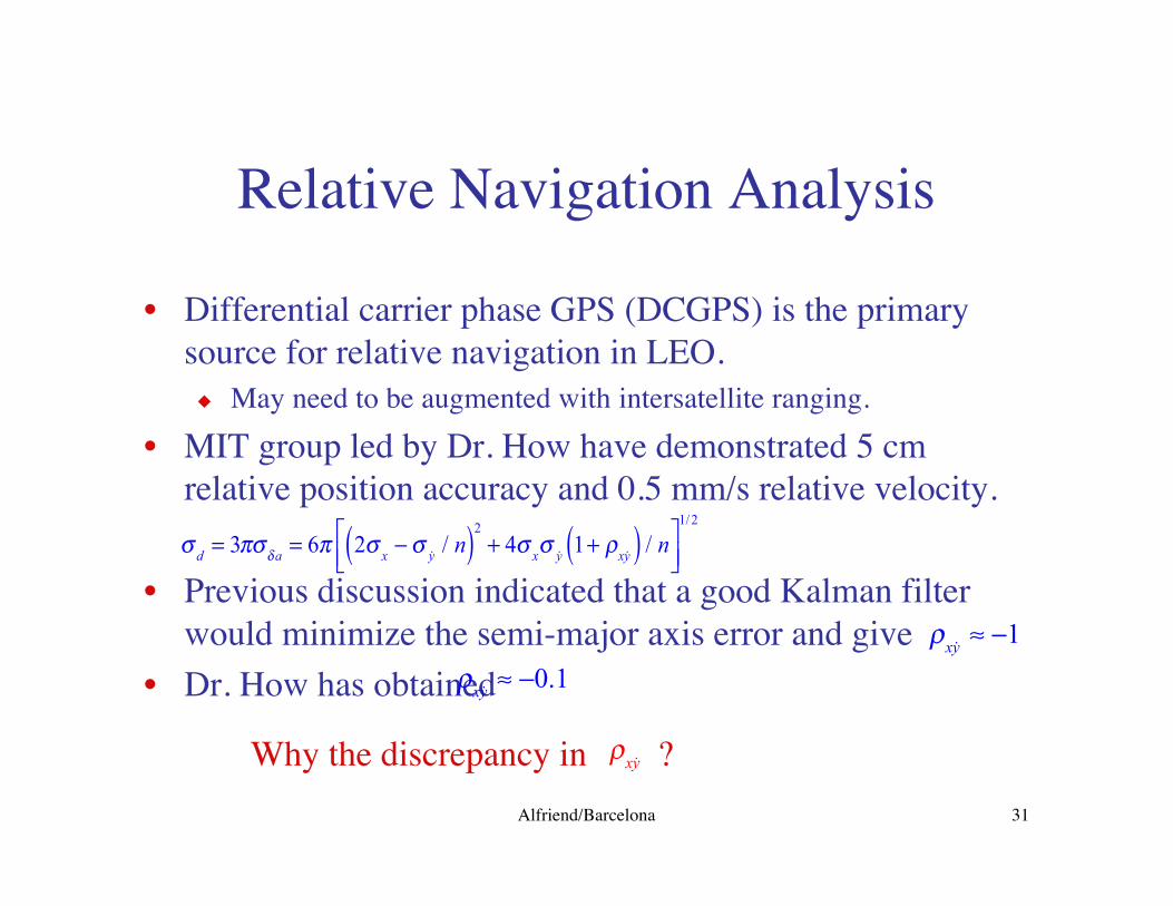
Relative Navigation Analysis
• Differential carrier phase GPS (DCGPS) is the primarysource for relative navigation in LEO.
u May need to be augmented with intersatellite ranging.• MIT group led by Dr. How have demonstrated 5 cm
relative position accuracy and 0.5 mm/s relative velocity.
• Previous discussion indicated that a good Kalman filterwould minimize the semi-major axis error and give
• Dr. How has obtained
s
d= 3ps d a
= 6p 2sx
- s &y / n( )2
+ 4sx
s &y 1 + rx&y( ) / nÈ
Î͢˚̇
1/ 2
r
x&y ª -1
r
x&y ª -0.1
Why the discrepancy in ? r
x&y

Alfriend/Barcelona 32
What are the physics?
• The coupling between x and ydot is at orbit rate.• The relative navigation filter is getting relative
position measurements at a much faster rate,approximately every 10-30 seconds.
• Due to the fast measurement rate the filter isbasically seeing three double integrators withweak coupling due to the orbit rate.
Can we prove this analytically?

Alfriend/Barcelona 33
Solution
&&x - 2n&y - 3n2x = vx
&&y + 2n &x = vy
x = x, &x, y, &y( )T
&x = Ax + Bvv = N 0,s v( ),E vvT( ) = Qc
z = Hx + w ,Measurement equationw = N 0,s w( ),E wwT( ) = Rc
H =1 0 0 00 0 1 0
È
ÎÍ
˘
˚˙
Let Dt be time between measurements and make the timetransformation
Letting the equations of motion become
t =t
Dt,( )¢ =
ddt
, ddt
=1
Dtddt
e = nDt
¢¢x = 2e ¢y + 3e 2x + Dt( )2 n x
¢¢y = -2e ¢x + Dt( )2 n y
Two weakly coupled double integrators
Alfriend/Barcelona 34
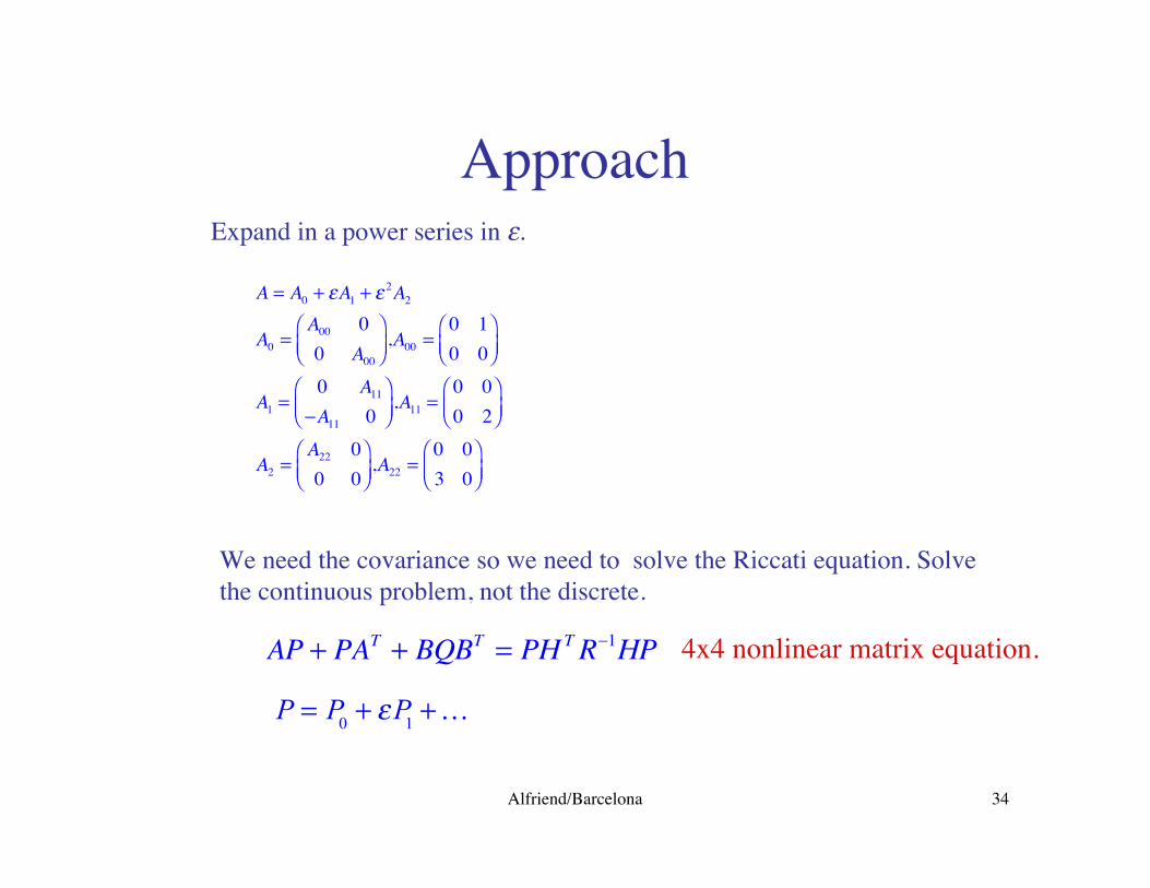
ApproachExpand in a power series in e.
A = A0 + e A1 + e 2A2
A0 =A00 00 A00
ÊËÁ
ˆ¯̃,A00 =
0 10 0
ÊËÁ
ˆ¯̃
A1 =0 A11
-A11 0ÊËÁ
ˆ¯̃,A11 =
0 00 2
ÊËÁ
ˆ¯̃
A2 =A22 00 0
ÊËÁ
ˆ¯̃,A22 =
0 03 0
ÊËÁ
ˆ¯̃
We need the covariance so we need to solve the Riccati equation. Solvethe continuous problem, not the discrete.
AP + PAT + BQBT = PH T R-1HP 4x4 nonlinear matrix equation.
P = P0
+ e P1
+ K

Alfriend/Barcelona 35
Approach (cont)P = P0 + eP1 + e 2P2 + ...
Po =P0xx 00 P0yy
ÊËÁ
ˆ¯̃.P0xx = P0yy =
P11 P12
P12 P22
ÊËÁ
ˆ¯̃
Pn =Pnxx Pnxy
PnxyT Pnyy
ÊËÁ
ˆ¯̃, n = 1,2,...
P0A1T + P1A0
T + A0P1 + A1P0 = P0DP1 + P1DP0
P1 A0T - DP0( ) + A0 - P0D( ) P1 = - P0A1
T + A1P0( )D =
C 02
02 CÊËÁ
ˆ¯̃,C =
1s wd
2
1 00 0
ÊËÁ
ˆ¯̃
At 0th order the problem is decoupled and P0xx=P0yy
Alfriend/Barcelona 36
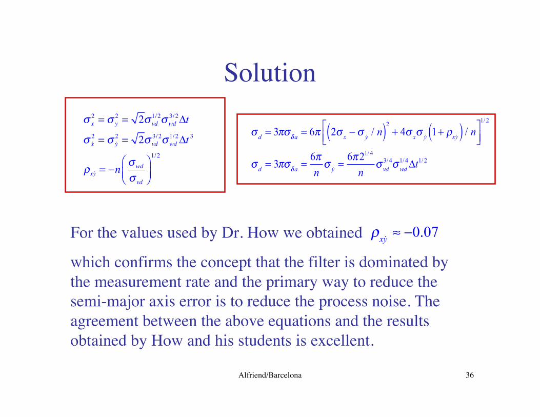
Solution
s x2 = s y
2 = 2s vd1/2s wd
3/2 Dt
s &x2 = s &y
2 = 2s vd3/2s wd
1/2 Dt 3
rx&y = -n s wd
s vd
ÊËÁ
ˆ¯̃
1/2
sd
= 3ps d a= 6p 2s
x- s &y / n( )2
+ 4sx
s &y 1 + rx&y( ) / nÈ
Î͢˚̇
1/ 2
sd
= 3ps d a=
6pn
s &y =6p 21/ 4
ns
vd3/ 4s
wd1/ 4Dt1/ 2
For the values used by Dr. How we obtained
which confirms the concept that the filter is dominated bythe measurement rate and the primary way to reduce thesemi-major axis error is to reduce the process noise. Theagreement between the above equations and the resultsobtained by How and his students is excellent.
r
x&y ª -0.07
Alfriend/Barcelona 37
Conclusions• Due to the fast measurement rate the relative navigation
filter basically sees three weakly coupled doubleintegrators.
• The semi-major axis error resulting from the DCGPSrelative navigation is almost strictly a function of thevelocity estimate error.
• To reduce the semi-major axis error we need to reduce theprocess noise, which is a function of the model error andmany errors in processing the GPS signals.
• The correlation coefficient will not approach (-1) asexpected unless the process noise is reduced several ordersof magnitude.

Alfriend/Barcelona 38
Results
-0.6
-0.5
-0.4
-0.3
-0.2
-0.1
0
0 1 2 3 4 5 6Position Error - cm
Cor
rela
tion
Coe
ffici
ent
sigv=10^(-7)sigv=5*10^(-7)sigv=10^(-6)sigv=5*10^(-6)sigv=10^(-5)
Dt=30
Alfriend/Barcelona 39
Constellation Control
Objective: Design a control law that counters theout-of-plane drift due to J2 and minimizes systemfuel consumption and balances the fuelconsumption over all the satellites in theformation
Alfriend/Barcelona 40
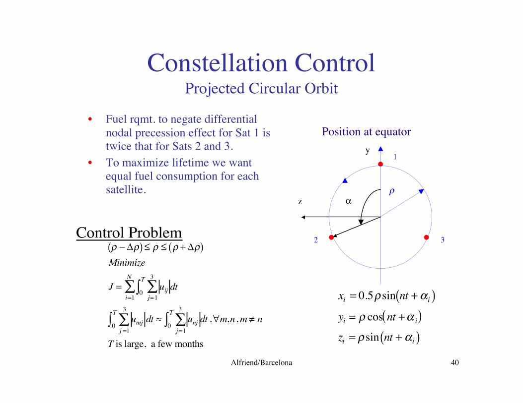
Constellation ControlProjected Circular Orbit
• Fuel rqmt. to negate differentialnodal precession effect for Sat 1 istwice that for Sats 2 and 3.
• To maximize lifetime we wantequal fuel consumption for eachsatellite. r
1
2 3
Position at equator
a
y
z
xi = 0.5r sin nt + ai( )yi = r cos nt + a i( )zi = r sin nt + ai( )
Control Problemr - Dr( ) £ r £ r + Dr( )
Minimize
J = uij dtj =1
3
Â0
T
Úi =1
N
Â
umj dtj =1
3
Â0
TÚ ª unj dt
j =1
3
Â0
TÚ ,"m,n , m π n
T is large, a few months
Alfriend/Barcelona 41
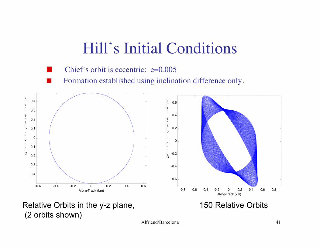
Hill’s Initial Conditionsn Chief’s orbit is eccentric: e=0.005n Formation established using inclination difference only.
-0.6 -0.4 -0.2 0 0.2 0.4 0.6
-0.4
-0.3
-0.2
-0.1
0
0.1
0.2
0.3
0.4
Along-Track (km)
Out-of-Plane (km)
Relative Orbits in the y-z plane, (2 orbits shown)
-0.8 -0.6 -0.4 -0.2 0 0.2 0.4 0.6 0.8
-0.6
-0.4
-0.2
0
0.2
0.4
0.6
Along-Track (km)
Out-of-Plane (km)
150 Relative Orbits
Alfriend/Barcelona 42
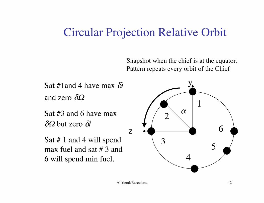
Circular Projection Relative Orbit
Sat #1and 4 have max di
and zero dW
Sat #3 and 6 have maxdW but zero di
Sat # 1 and 4 will spendmax fuel and sat # 3 and6 will spend min fuel.
Snapshot when the chief is at the equator.Pattern repeats every orbit of the Chief
y
z
1
34
2
5
6
a

Alfriend/Barcelona 43
Constellation Control Concept
Balance the fuelconsumption over acertain period byrotating all the deputiesby an additional rate
Snapshot when the chief is atthe equator.
y
z
1
3
4
2
5
6
a
&a

Alfriend/Barcelona 44
Modified Hill’s Equations
&&x - 2nxy
&y - 3nxy2 x = u
x
&&y + 2nxy
x = uy
&&z + n 2z = uz
+ 2An cosa sin[nt]
A =3
2r J
2 n
0
Re
R
Ê
ËÁˆ
¯̃
2
sin2 i
Assume no in-track driftcondition satisfied.
n Æ n + &aThe near-resonance in the z-axis is detuned byintroducing an additional rotation.
Alfriend/Barcelona 45
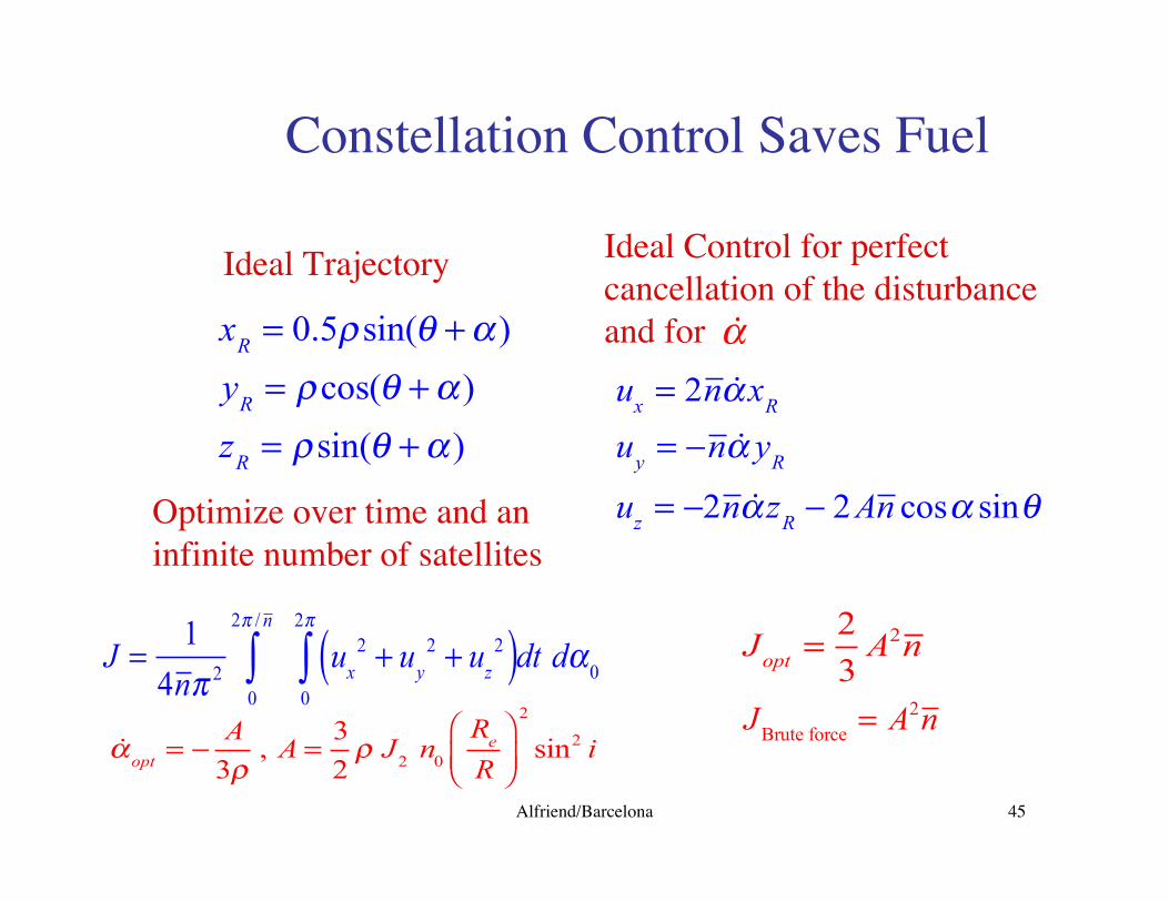
Constellation Control Saves Fuel
xR
= 0.5r sin(q + a )
yR
= r cos(q + a )
zR
= r sin(q + a )
Ideal Trajectory
&a
Ideal Control for perfectcancellation of the disturbanceand for
ux
= 2n &a xR
uy
= -n &a yR
uz
= -2n &a zR
- 2An cosa sinqOptimize over time and aninfinite number of satellites
J =
1
4np 20
2p / n
Ú ux
2 + uy
2 + uz
2( )0
2p
Ú dt da0
&a
opt= -
A
3r, A =
3
2r J
2 n
0
Re
R
Ê
ËÁˆ
¯̃
2
sin2 i
J
opt=
2
3A2n
J
Brute force= A2n
Alfriend/Barcelona 46
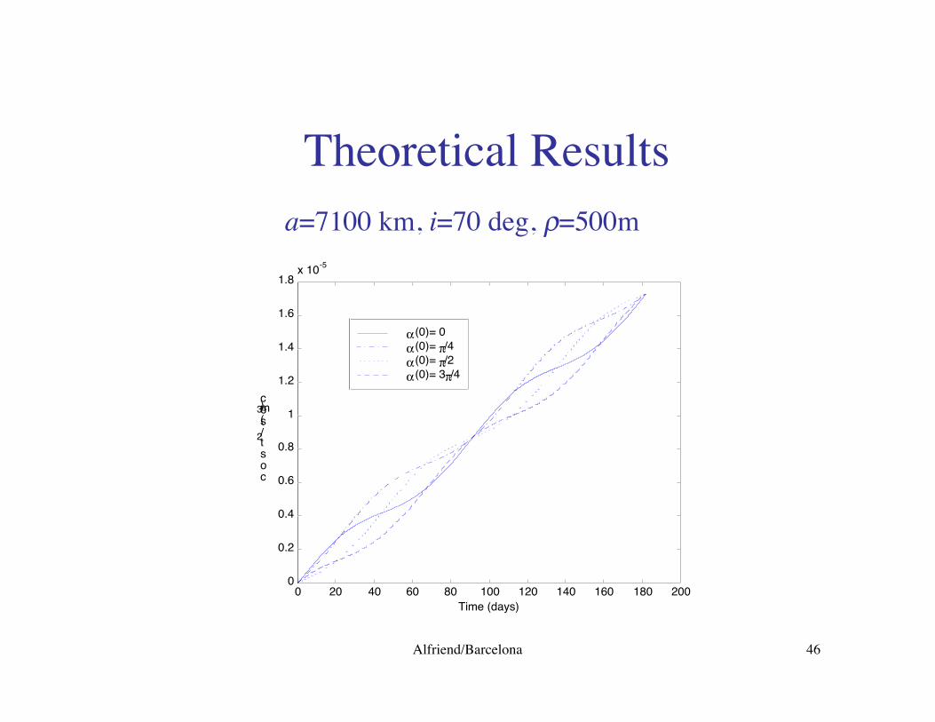
Theoretical Results
0 20 40 60 80 100 120 140 160 180 2000
0.2
0.4
0.6
0.8
1
1.2
1.4
1.6
1.8x 10⁻⁵
Time (days)
cost (m
2/sec
3)
a(0)= 0a(0)= p/4a(0)= p/2a(0)= 3p/4
a=7100 km, i=70 deg, r=500m
Alfriend/Barcelona 47
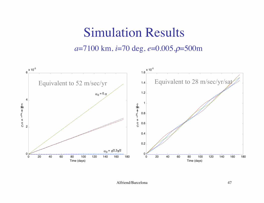
Simulation Results
0 20 40 60 80 100 120 140 160 1800
0.2
0.4
0.6
0.8
1
1.2
1.4
1.6x 10⁻⁵
Time (days)
Cost (m
2/sec
3)
a=7100 km, i=70 deg, e=0.005,r=500m
0 20 40 60 80 100 120 140 160 1800
0.2
0.4
0.6
0.8
1
1.2
1.4
1.6x 10⁻⁵
Time (days)
Cost (m
2/sec
3)
Equivalent to 28 m/sec/yr/sat
0 20 40 60 80 100 120 140 160 1800
2
4
6x 10⁻⁵
Time (days)
Cost (m
2/sec
3)
a0 = 0,p
a0 = p/2,3p/2
Equivalent to 52 m/sec/yr

Alfriend/Barcelona 48
Simulation Results
-5 -4.5 -4 -3.5 -3 -2.5 -2 -1.5 -1 -0.5 02.4
2.6
2.8
3
3.2
3.4
3.6
3.8
4
4.2x 10⁻⁴
adot (deg/day)
Total Cost (m
2/sec
3/yr)

Alfriend/Barcelona 49
Formation Control Comments
• Use of orbital elements in formation design and formationcontrol offers distinct advantages over the Cartesian frame.However, relative navigation measurements will be in theCartesian frame.
• The control problem should address the real problem, notthe mathematically easy problem.
• With current technology formation control usingcontinuous control is probably not feasible due to the lowthrust levels.