ISSN 1795-5300

MTT Discussion Papers 4 • 2009MTT Discussion Papers 4 • 2009

Dynamically Optimal Phosphorus Management

and Agricultural Water Protection

Antti Iho & Marita Laukkanen

Dynamically Optimal Phosphorus Management and

Agricultural Water Protection

Antti Iho and Marita Laukkanen*

Abstract

This paper puts forward a model of the role of phosphorus in crop production, soil

phosphorus dynamics and phosphorus loading that integrates the salient economic and

ecological features of agricultural phosphorus management. The model accounts for

the links between phosphorus fertilization, crop yield, accumulation of soil

phosphorus reserves, and phosphorus loading. It can be used to guide precision

phosphorus management and erosion control as means to mitigate agricultural

loading. Using a parameterization for cereal production in southern Finland, the

model is solved numerically to analyze the intertemporally optimal combination of

fertilization and erosion control and the associated soil phosphorus development. The

optimal fertilizer application rate changes markedly over time in response to changes

in the soil phosphorus level. When, for instance, soil phosphorus is initially above the

socially optimal steady state level, annually matching phosphorus application to the

prevailing soil phosphorus stock produces significantly higher social welfare than

using a fixed fertilizer application rate. Erosion control was found to increase welfare

only on land that is highly susceptible to erosion.

Keywords: precision nutrient management, agricultural phosphorus loading, cereal

production, soil phosphorus reserves, agricultural water pollution, dynamic

programming

Agrifood Research Finland, Luutnantintie 13, 00410 Helsinki, Finland. Email addresses:

antti.iho@mtt.fi, marita.laukkanen@mtt.fi.

2

1 Introduction

Phosphorus loading from agricultural land has been identified as one of the major

causes of surface water quality problems in developed countries (Sharpley and

Rekolainen 1997, Shortle and Abler 1999, HELCOM 2004, Ekholm et al. 2005). One

fundamental cause of phosphorus loading is inefficiency in fertilizer use. The yield

response to phosphorus consists of the impacts of the phosphorus fertilizer applied in

the current year and the phosphorus accumulated in the soil. Soil phosphorus largely

determines the crop response to phosphorus and in increasing quantities reduces the

yield response to fertilizer. When phosphorus fertilization exceeds the removal of

phosphorus by the crop, most of the surplus phosphorus will remain in the soil to add

to the phosphorus reserve (Hooda et al. 2001). Soils with excessive phosphorus

reserves in turn pose the highest risk to the environment (Yli-Halla et al. 1995).

Phosphorus loading can be mitigated by applying phosphorus fertilizers to the

production process with greater precision as well as by reducing soil loss (e.g. catch

crops, vegetative filter strips, reduced tillage). Precision phosphorus management

requires knowledge about links between phosphorus fertilization, crop yield,

accumulation of soil phosphorus reserves, and phosphorus loading. Efficient policies

to control agricultural phosphorus loading should in turn weigh the trade-off between

profits from production and the environmental damage from phosphorus loading over

time.

The literature on the optimal management of phosphorus has not fully accounted for

the complex dynamics governing phosphorus loading.1 Schnitkey and Miranda (1993)

analyzed optimal steady state manure and mineral fertilizer application rates under

alternative phosphorus control policies and found that soil phosphorus reserves affect

crop yield only. The study does not model the link between phosphorus loss and

phosphorus reserves explicitly; rather, pollution is controlled through exogenous

limits on annual manure and commercial fertilizer application. Goetz and Zilberman

1 There is a more extensive literature on optimal phosphorus fertilization from the point of view of soil

fertility alone, that is, where the externality arising from phosphorus loss to the environment is not

considered. Kennedy (1986) provides an overview of the numerical dynamic methods applied to such

problems. Lambert et al. (2007) is a recent study that estimated site-specific crop response functions

with a nutrient carry-over equation using on-farm agronomic data. Estimates were used in a dynamic

programming model to determine optimal site-specific fertilizer policies and soil phosphorus evolution.

3

(2000) determined spatially and intertemporally optimal mineral fertilizer application

rates, number of animal units, proportion of total manure applied to the soil, and

phosphorus concentration in the receiving body of water. While their model accounts

for the complex dynamic and spatial characteristics of phosphorus loading, it makes

no provision for the dynamic development of soil phosphorus reserves in response to

fertilizer application; the initial soil phosphorus level in each location is incorporated

into a fixed phosphorus index. Goetz and Keusch (2005) analyzed farmers’ choices of

crop rotation, fertilizer type and tillage practice. They consider soil loss as the primary

externality associated with agricultural production. Phosphorus loss is determined by

soil loss alone, with the impact of soil phosphorus level on phosphorus loading not

accounted for. Iho (2007) incorporated the control of erosion and soil phosphorus

reserves as means to mitigate phosphorus loading. He derived optimal steady state

policies for phosphorus fertilization and erosion control but did not analyze how soil

phosphorus and optimal policies evolve over time, leaving open the question of how

to adjust phosphorus application in response to changing field conditions.

This article extends the previous research on agricultural phosphorus management by

considering the optimal development of soil phosphorus reserves over time; in

particular, it accounts for the dual role of soil phosphorus in accelerating crop growth

and phosphorus losses. We develop a framework for analyzing the intertemporally

optimal combination of fertilization and erosion control policies and the associated

soil phosphorus development. To study precision phosphorus management in a

realistic setting, we employ a numerical example that allows us to work with a state-

of-the-art ecological description. The example is based on cereal production in

southern Finland, but the elements of the application are common to phosphorus

management in agriculture worldwide. With the empirical components matched to

local conditions, the model can be used in combination with soil phosphorus testing to

guide precision phosphorus management and reduce the generation of polluting

phosphorus residues. Our results indicate that adjusting phosphorus fertilization in

response to changes in soil phosphorus levels is crucial in designing efficient

phosphorus policies. The optimal fertilization rate changes markedly over time in

response to changes in the soil phosphorus status. Matching fertilizer application to

field conditions was found to be especially important when depleting particularly high

soil phosphorus reserves: even following a privately optimal depletion path, which

4

does not account for environmental damage from phosphorus loading, may produce

smaller efficiency losses than following a fixed fertilizer application rate set equal to a

socially optimal steady state level.

2 The modeling framework

Consider a field parcel bordering a waterway. For simplicity, we assume that the

parcel is square in shape and measures one hectare. A single crop is produced using

phosphorus fertilizer as a variable input. The per hectare production function is

( , )t tY s x , where ts denotes accumulated soil phosphorus and tx phosphorus fertilizer

applied in the current period. The soil phosphorus level changes from one period to

the next according to the state transition function 1 ( , )t t ts s x+ = Γ . The product and

input prices are denoted by p and w, respectively, and are assumed to be constant.

Operational costs per hectare are denoted by FC and include costs such as seeds, labor

and the rental or annualized cost of machinery.

Accumulated soil phosphorus and soil loss through erosion cause phosphorus loading

from the field to the adjacent waterway. Phosphorus transport from fields to surface

waters occurs in two main forms: dissolved phosphorus (DP) and particulate

phosphorus (PP). The main determinant of DP loss is accumulated soil phosphorus,

whereas PP loss is governed by erosion. Soil phosphorus also affects the

bioavailability of PP (Sharpley 1993, Uusitalo et al. 2003).2 In our model, total

phosphorus load per hectare includes DP load and the bioavailable fraction of PP

load. We consider two means of reducing phosphorus loading at source: precision

phosphorus fertilizer application, where application rates are adjusted annually based

on the current soil phosphorus level, and vegetative filter strips (VFS) as a measure to

mitigate erosion. The erosion susceptibility of land is indexed by field slope γ (see

e.g. Wischmeier and Smith 1978). The total phosphorus load is then given by

( , , )t tL s b γ , where tb is the VFS width, which by assumption can be chosen annually.

For the hectare-sized square parcel considered here, the VFS width also determines

2 Bioavailability describes the fraction of phosphorus that can be used by algae and that thus

contributes to eutrophication. The bioavailability of PP has been estimated to range from 20 to 60

percent (see e.g. Sharpley 1993), while DP is considered fully bioavailable (see e.g. Ekholm and

Krogerus 2003).

5

the area of the VFS. The cost of planting and maintaining filter strips is given by

( )tC b . This includes the costs of seed as well as the machinery and labor required for

planting and for removing plant residues. The per-period monetary damage resulting

from phosphorus loading is denoted by ( )( , , )t tD L s b γ . The per-period, per-hectare

profit from crop production is given by

( ) [ ], , ( , ) (1 ) ( )t t t t t t t ts x b pY s x wx FC b C bπ = − − − − . (1)

Multiplication by the term (1 )tb− in (1) accounts for the fact that conversion of a

fraction of arable land tb into a vegetative filter removes that area from production.

3 Dynamics of the phosphorus management problem

We are concerned with socially efficient fertilization and filter strip policies over

time. Other inputs are assumed to be fixed. We assume that a social planner exists.

The social planner’s problem is to maximize the present discounted value of rewards

from production, equal to profits net of environmental damage. The farmer’s problem

is limited to the present discounted value of profits. The social planner’s discrete-

time, continuous-state decision problem is given by

( ) ( ){ },

0

max , , ( , , ) t t

t

t t t t tx b

t

s x b D L s bβ π γ∞

=

− ∑ (2)

subject to

1 0 0( , ), = , t t ts s x s S+ = Γ

0, 0 1,t tx b≥ ≤ ≤

where β is the discount factor corresponding to the social discount rate δ , with

1

1β

δ=

+, and the parameter 0S denotes the initial soil phosphorus level. The

6

farmer’s intertemporal optimization problem is identical to that described by

equations (2) and (3) with the exception of the term ( )( , , )t tD L s b γ .

Consider first the social planner’s problem. Denote by ( )V s the maximum attainable

sum of current and future net benefits given a current soil phosphorus level of s.

Bellman’s (1957) principle of optimality implies that the optimal policy must satisfy

the functional equation

( )( ) ( )( ){ },

( ) max ( , , ) , , ,x b

V s s x b D L s b V s xπ γ β= − + Γ . (3)

The optimal fertilization rate x and filter strip width b for each level of soil test

phosphorus s must satisfy

( )( , , ) ( , ) ( , ) 0x xs x b s x s xπ βλ+ Γ Γ = (4)

( )( , , ) ( , , ) ( , ) 0.b L bs x b D L s b L s bπ γ− = (5)

The envelope theorem applied to the same problem implies

( ) ( ) ( )( , , ) ( , , ) ( , , ) ( , ) ( , )s L S ss s x b D L s b L s b s x s xλ π γ γ βλ= − + Γ Γ . (6)

The equilibrium conditions do not involve the value function but its derivative

( ) ( )s V sλ ′≡ , the shadow value of the soil phosphorus reserves. The first-order

condition (4) states for an interior solution that at every soil phosphorus level fertilizer

should be applied to the point where the sum of its marginal impact on profits in the

current period and the marginal impact on the discounted value of the phosphorus

reserve in the next period equals zero. Because the VFS does not affect the transition

process, the partial derivative Γb is zero and the first-order condition (5) for VFS

width collapses into a static optimality condition. The filter strip width should be

chosen so that the marginal reduction in profits from production equals the marginal

reduction in the damage costs associated with phosphorus loading. Equation (6)

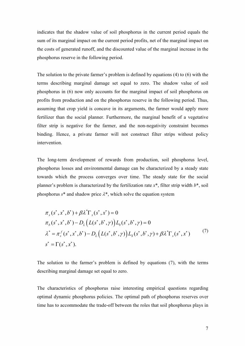
7

indicates that the shadow value of soil phosphorus in the current period equals the

sum of its marginal impact on the current period profits, net of the marginal impact on

the costs of generated runoff, and the discounted value of the marginal increase in the

phosphorus reserve in the following period.

The solution to the private farmer’s problem is defined by equations (4) to (6) with the

terms describing marginal damage set equal to zero. The shadow value of soil

phosphorus in (6) now only accounts for the marginal impact of soil phosphorus on

profits from production and on the phosphorus reserve in the following period. Thus,

assuming that crop yield is concave in its arguments, the farmer would apply more

fertilizer than the social planner. Furthermore, the marginal benefit of a vegetative

filter strip is negative for the farmer, and the non-negativity constraint becomes

binding. Hence, a private farmer will not construct filter strips without policy

intervention.

The long-term development of rewards from production, soil phosphorus level,

phosphorus losses and environmental damage can be characterized by a steady state

towards which the process converges over time. The steady state for the social

planner’s problem is characterized by the fertilization rate x*, filter strip width b*, soil

phosphorus s* and shadow price λ*, which solve the equation system

( )( )

*

* *

( , , ) ( , ) 0

( , , ) ( , , ) ( , , ) 0

( , , ) ( , , ) ( , , ) ( , )

( , ).

x x

b L b

f

s L S s

s x b s x

s x b D L s b L s b

s x b D L s b L s b s x

s s x

π βλ

π γ γ

λ π γ γ βλ

∗ ∗ ∗ ∗ ∗

∗ ∗ ∗ ∗ ∗ ∗ ∗

∗ ∗ ∗ ∗ ∗ ∗ ∗ ∗ ∗

∗ ∗ ∗

+ Γ =

− =

= − + Γ

= Γ

(7)

The solution to the farmer’s problem is defined by equations (7), with the terms

describing marginal damage set equal to zero.

The characteristics of phosphorus raise interesting empirical questions regarding

optimal dynamic phosphorus policies. The optimal path of phosphorus reserves over

time has to accommodate the trade-off between the roles that soil phosphorus plays in

8

both crop growth and environmental degradation. If the initial soil phosphorus level is

above the socially optimal level, what is the optimal mix of abatement through

depletion of soil phosphorus reserves and erosion control? Does the ranking of the

two abatement measures change along the optimal path, and how is this ranking

influenced by the key ecological characteristics of the site, such as susceptibility to

erosion? To study these questions in a realistic setting, we construct a detailed

bioeconomic model of crop production and phosphorus loading, with barley as the

sample crop, and empirically evaluate optimal dynamic phosphorus policies.

4 Bioeconomic model and empirical illustration

Matching fertilizer application rates to soil phosphorus levels requires knowledge

about the crop production and pollution generation processes. Our bioeconomic model

considers the impact of soil phosphorus and phosphorus fertilization on yield and the

accumulation of soil phosphorus as well as the link from soil phosphorus to

phosphorus loading. The model is parameterized for sandy clay soils in southern

Finland. We consider three representative field slopes: 0.5%, 2% and 7%. The

average slope is 0-1% for some 57% of parcels in Finland; 1-3% for 26% of parcels;

and greater than 7% for 3% of parcels (Puustinen et al. 1994). While the proportion of

steeply sloped parcels is small, we include a steep slope in the analysis as an example

of land with particularly high runoff potential. Throughout the empirical illustration,

soil phosphorus level is expressed as agronomic soil test phosphorus (STP).

4.1 Crop production function

The yield response to phosphorus consists of the impacts of the fertilizer applied and

the phosphorus accumulated in the soil. Following Myyrä et al. (2007), we specify the

phosphorus response function for barley as

3 6 71 2 4 5 8

( )( , ) (1 ) ( )

YY Y

sY Y Y Y Yx xY s x e s x

s

α α αα α α α α− −

= − + − + + . (8)

9

From Myyrä et al. (2007), the parameter values for barley production in southern

Finland are 1

Yα = 3367, 2

Yα = 0.74, 3

Yα = 0.37, 4

Yα = 21.7, 5

Yα = 0.414, 6

Yα = 17.01,

7

Yα = 0.1817 and 8

Yα = 5.856.

4.2 Transition function for soil phosphorus

Ekholm et al. (2005) model the relationship between the development of soil

phosphorus and the phosphorus surplus, that is, the fertilizer applied to the land but

not utilized by the crop. The phosphorus surplus is defined by

( ), ( ) ( , )balP s x x s Y s x= −Λ , where ( )sΛ is the phosphorus concentration of the crop

yield. Saarela et al. (1995) provide information that allows specification of the

phosphorus concentration of crop yield as a logarithmic function of the soil

phosphorus. Following Ekholm et al. (2005), the change in soil phosphorus from one

year to the next is then specified as follows:

( ) ( ) ( )1 2 3 4 5, ln( ) ( , )s x s s x s Y s xα α α α αΓ Γ Γ Γ Γ Γ = + + − + , (9)

where the term ( )4 5ln( ) ( , )x s Y s xα αΓ Γ − + is the phosphorus surplus and the term

4 5ln( )sα αΓ Γ+ defines the phosphorus concentration of the crop yield. The parameter

estimates 1αΓ = 0.9816, 2α

Γ = 0.0032 and 3αΓ = 0.00084 were obtained directly from

Ekholm et al. (2005).3 The parameter estimates 4α

Γ = 0.000186 and 5αΓ = 0.003 were

obtained from data in Saarela et al. (1995) through ordinary least squares estimation.4

4.3 Phosphorus load and abatement using vegetative filter strips

The phosphorus load function ( , , )t tL s b γ expresses DP load and the bioavailable

fraction of PP load net of VFS abatement. Following Uusitalo and Jansson (2002), the

3 The transition function presented by Ekholm et al. (2005) depicts changes in STP with a time step of

10-15 years with a constant phosphorus surplus over the period. Using a one-year time step predicts

STP values in the long run that differ slightly from those predicted by the Ekholm et al. (2005)

equation. For initial STP levels ranging from 2 to 40 mg l-1

and P surpluses from -5 to 25 kg ha-1

y-1

, the

differences in STP values for year 30 predicted by equation (10) with a constant phosphorus surplus

and one- and ten-year time steps were 0 to 8%. 4 The phosphorus concentration data in Saarela et al. (1995) were measured from dry matter. Their data

were made commensurate with storage weight yield prior to the estimation.

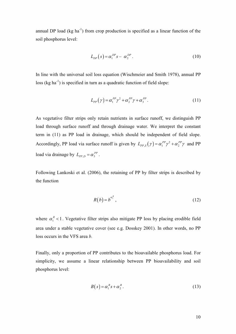
10

annual DP load (kg ha-1

) from crop production is specified as a linear function of the

soil phosphorus level:

( ) 1 2– DP DP

DPL s sα α= . (10)

In line with the universal soil loss equation (Wischmeier and Smith 1978), annual PP

loss (kg ha-1

) is specified in turn as a quadratic function of field slope:

( ) 2

1 2 3

PP PP PP

PPL γ α γ α γ α= + + . (11)

As vegetative filter strips only retain nutrients in surface runoff, we distinguish PP

load through surface runoff and through drainage water. We interpret the constant

term in (11) as PP load in drainage, which should be independent of field slope.

Accordingly, PP load via surface runoff is given by ( ) 2

, 1 2

PP PP

PP SL γ α γ α γ= + and PP

load via drainage by , 3

PP

PP DL α= .

Following Lankoski et al. (2006), the retaining of PP by filter strips is described by

the function

( ) 1R

R b bα

= , (12)

where 1 1Rα < . Vegetative filter strips also mitigate PP loss by placing erodible field

area under a stable vegetative cover (see e.g. Dosskey 2001). In other words, no PP

loss occurs in the VFS area b.

Finally, only a proportion of PP contributes to the bioavailable phosphorus load. For

simplicity, we assume a linear relationship between PP bioavailability and soil

phosphorus level:

( ) 1 2

B BB s sα α= + . (13)

11

From (10)-(13), the total bioavailable phosphorus load is given by

( ) ( ) ( )( ) ( )( ) ( ), ,, , 1 1DP PP D PP SL s b L s B s b L R b Lγ γ = + − + − . (14)

The parameter estimates 1

DPα = 0.0567 and 2

DPα = 0.0405 for equation (10) were

obtained by multiplying the estimates of DP concentration in mg l-1

in Uusitalo and

Jansson (2002) by an estimated runoff volume of 270,000 l ha-1

(Ekholm et al. 2005)

and converting the units to kg ha-1

. The data in Uusitalo et al. (2007) produce

parameter estimates of 1 0.035PPα = , 2 0.12PPα = and 3 0.37PPα = for equation (11).

The parameter value 1 0.3Rα = was obtained from Lankoski et al. (2006), who used

results from a Finnish study on grass filter strips (Uusi-Kämppä and Kilpinen 2000) in

calculating their estimate. The data in Uusitalo et al. (2003) yield parameter estimates

of 1 0.48Bα = and 2 19.7 Bα = for equation (13).

4.4 Damage from phosphorus loading

Following Gren and Folmer (2003), damage from phosphorus loading is described by

the function

( )( ) ( )1, , , , .DD L s b L s bγ α γ= (15)

Gren and Folmer estimated the constant marginal damage from nitrogen loading in

the Baltic Sea countries. We use their estimate and multiply phosphorus loading by

the Redfield ratio of 7.2 to convert it into nitrogen equivalents, which yields the

parameter value 1 47Dα = (EUR kg-1

).

4.5 Prices and costs

Product price p and input price w, obtained from Myyrä et al. (2007), are 0.11 € kg-1

and 1.22 € kg-1

, respectively. The annual fixed costs of production, FC, were

obtained from Helin et al. (2006) and equal 113 € ha-1

. The costs of establishing a

vegetative filter strip derive primarily from removing plant residue each year in order

12

to prevent phosphorus in the residue from leaching into the environment. The VFS

cost function thus takes the form

( ) 1

CC b bα= . (16)

Palva (2003) and Pentti and Laaksonen (2005) estimated the costs in Finland to be 31

€ ha-1

for mowing and 65 € ha-1

for baling and transportation, yielding a total of 1

Cα =

96 € ha-1

. Finally, the discount rate was set at 5%.

4.6 Solution method

To determine the optimal phosphorus control policies over time, the dynamic program

in (3) was solved numerically using the collocation method. This technique involves

writing the value function approximant as a linear combination of n known basis

functions φ1, φ2, …, φn whose coefficients c1, c2, …, cn are determined by the

equation

( ) ( )1

n

j j

j

V s c sφ

=

≈∑ (17)

The coefficients c1, c2, …, cn are defined by requiring the value function approximant

to satisfy the Bellman equation (3) at a finite set of collocation nodes. The solution

was implemented using the CompEcon Toolbox for Matlab.5 The solution produces

policy functions for ( )x s and ( )b s that provide a mapping from the current soil

phosphorus level to the optimal fertilization and VFS policies.

5 The Matlab code is available from the authors upon request. The CompEcon Toolbox is a library of

Matlab functions, developed to accompany Miranda and Fackler (2002), for numerically solving

problems in economics and finance . The library is downloadable at

http://www4.ncsu.edu/~pfackler/compecon/toolbox.html.

13

5 Results

5.1 Base parameterization

Optimal steady state outcomes

Table 1 displays the socially and privately optimal steady state outcomes. The socially

optimal steady state soil phosphorus level and phosphorus application rate are almost

equal across the three field slopes considered. By contrast, the socially optimal VFS

width differs notably across slopes. For the moderately sloped and level fields, the

optimal steady state VFS width is practically zero (0.06 meters). For the steepest

slope, the optimal VFS width is 0.6 meters, which produces an overall abatement of

15% in bioavailable phosphorus loss. As slope only affects phosphorus runoff, which

does not enter the farmer’s objective function, it has no impact on the privately

optimal solution. The steady state phosphorus application rate is 5-6% above the

socially optimal level, and no VFSs are constructed. The privately optimal soil

phosphorus level exceeds the socially optimal value by 16-18%, depending on field

slope. The impact of field slope on phosphorus loading is apparent in the results. Even

with erosion control, the bioavailable phosphorus loading from the steepest slope is

twice as high as that from the most level slope. The bioavailable fraction of PP is not

very sensitive to soil phosphorus level and remains at approximately 23% for all the

outcomes reported in Table 1.

Table 1. Socially and privately optimal steady state outcomes for the base

parameterization.

Fertilization

kg/ha

VFS

m

Soil P

mg/l

PP load

kg/ha

DP load

kg/ha

Bioavailable P load

kg/ha/year

Social optimum

Slope 0.5% 24.4 0 6.1 0.44 0.31 0.41

Slope 2% 24.4 0.06 6.1 0.71 0.31 0.47

Slope 7% 24.1 0.60 6.0 2.35 0.30 0.83

Private optimum

Slope 0.5% 25.6 0 7.3 0.44 0.37 0.47

Slope 2% 25.6 0 7.3 0.75 0.37 0.55

Slope 7% 25.6 0 7.3 2.97 0.37 1.0

14

Optimal policy functions

Figure 1 shows the socially optimal fertilization rate and filter strip width as functions

of the current soil phosphorus level. For all three slopes considered, the optimal

fertilization rate is sensitive to the current soil phosphorus status, ranging from 0 to 70

kg/ha/year for soil phosphorus levels between 2 and 26 mg/l. By contrast, slope has

no noticeable effect on the rate. The result reflects the role of phosphorus in crop

production: crop response is dependent primarily on soil phosphorus level, while the

annual fertilization rate is chosen mainly to control soil phosphorus reserves. Field

slope is a determinant of optimal VFS width, however: for the small and moderate

slopes (0.5 and 2%), the optimal VFS width is practically zero regardless of the soil

phosphorus level. Erosion control becomes important in the case of the steep slope

(7%), with the optimal VFS width ranging from 0.6 to 1.2 meters. The results for the

private farmer are qualitatively similar to those in Figure 1, but the VFS width

remains zero for all soil phosphorus levels and all field slopes. Nevertheless, the

optimal fertilizer application rate changes markedly as field phosphorus status

changes, even with environmental damage excluded from the objective function.

The optimal VFS policy on a steeply sloped field is non-monotonic in soil phosphorus

level: filter strips are wider when the phosphorus reserves are either very low or very

high. The two opposite forces producing this result are the opportunity cost of land

and the bioavailability of PP load. Constructing VFSs requires setting land aside from

production. When the soil phosphorus reserve is low, land is relatively unproductive

and the opportunity cost of establishing VFSs is low. At the same time, the optimal

fertilization rate is high, increasing the need to reduce runoff by planting VFSs where

effective. As the soil phosphorus level increases, fertilization decreases along the

optimal path, and the cost of VFSs increases, resulting in an initial decrease in the

optimal VFS width. On the other hand, the bioavailability of PP increases linearly

with soil phosphorus, heightening the importance of erosion control on steeply sloped

fields and resulting in an eventual increase in the optimal VFS width. For the small

and moderate slopes, the optimal VFS width decreases with soil phosphorus for the

range considered here.

15

5 10 15 20 250

10

20

30

40

50

60

70Optimal Fertilization Rate

Soil Phosphorus Level (mg/l)

Fertilization (kg/ha)

5 10 15 20 250

0.2

0.4

0.6

0.8

1

1.2

1.4

1.6

1.8

2Optimal Filter Strip Width

Soil Phosphorus Level (mg/l)

Filter Strip W

idth (m)

Slope 0.5%

Slope 2%

Slope 7%

Steady States

Figure 1. Optimal fertilizer application rate and vegetative filter strip width as

functions of soil phosphorus.

Optimal paths to the socially optimal steady state

The previous section discussed optimal fertilization rate and VFS width as functions

of the current soil phosphorus level. We next consider optimal depletion of excessive

soil phosphorus reserves where the social planner takes over the management of land

previously managed by a private farmer. Here the focal questions to be addressed are:

How fast is soil phosphorus driven towards its new steady state value, and how do the

optimal fertilization rate and VFS width evolve over time? What would be the

associated reduction in phosphorus loading, relative to the load in the privately

optimal solution? Figure 2 illustrates the optimal state and policy paths, with the

initial soil phosphorus level set equal to the privately optimal steady state value of 7.3

mg/l.

16

0 20 40 6010

15

20

25Fertilization Paths

Year

Fertilization (kg/ha)

0 20 40 606

6.5

7

7.5Soil Phosphorus Paths

Year

Soil Phosphorus (mg/l)

0 20 40 600

0.2

0.4

0.6

0.8Filter Strip Paths

Year

Filter Strip W

idth (m)

0 20 40 600

10

20

30Phosphorus Abatement Paths

Year

Abatement (%

)

Slope 0.5%

Slope 2%

Slope 7%

Figure 2. Socially optimal state and control paths and the associated phosphorus

abatement. The initial soil phosphorus level is equal to the privately optimal steady

state value of 7.3 mg/l.

While the socially and privately optimal steady state fertilization levels differ little,

the privately optimal steady state soil phosphorus level is 16-18% above the socially

optimal level; the discrepancy between the two solutions increases with field slope. In

the initial years of depletion, the socially optimal policy actively drives the soil

phosphorus reserve towards its socially optimal level. Fertilization is first reduced to

less than 15 kg/ha/year to induce a rapid decline in the phosphorus reserves. As the

excessive reserves are depleted, the fertilization rate increases towards its optimal

steady state level. Depleting the soil phosphorus reserves nevertheless takes time,

even though in absolute terms the difference between the socially and privately

optimal steady state soil phosphorus levels is on the order of 1 mg/l. The socially

optimal steady state reserve level is only reached some 20 to 40 years after the

beginning of depletion. A VFS would in practice only be planted on the steep slope of

7%, and the optimal VFS width remains almost unchanged for the period considered.

If a VFS is implemented, the environmental benefits of intensified erosion control are

17

realized immediately, with abatement at approximately 12%. Contrastingly,

abatement through depleted soil phosphorus is achieved slowly; there are no fast ways

to reduce phosphorus loading from level or moderately sloped fields.

Comparison of the socially optimal dynamic solution, fixed fertilizer application

rates, and the privately optimal dynamic solution

There are many ways to deplete the soil phosphorus reserve towards its socially

optimal level. To illustrate the impact of optimally adjusting fertilizer application in

response to changes in the soil phosphorus level, we considered a simple fixed policy

rule as an alternative: in all periods, apply fertilizer at a rate equal to the socially

optimal steady state level. The fixed policy rule reflects a situation where the social

planner has the knowledge to determine the optimal steady state, but not the optimal

adjustment path. Adjusting the policy may also be politically infeasible. Table 2

displays the present value of social welfare for the first hundred years of the socially

optimal dynamic solution, the fixed fertilization rule, and the privately optimal

dynamic solution; the initial soil phosphorus level is set equal to the privately optimal

steady state value of 7.3 mg/l. Efficiency losses from following a suboptimal policy

were computed as a percentage change relative to the welfare from the socially

optimal solution. The differences in the overall level of welfare between the optimal

dynamic solution and the fixed policy rule are negligible, due to the small difference

between the initial and the optimal steady state soil phosphorus levels. Thus, where

the existing soil nutrient stock is close to the target level, a fixed fertilizer application

rate performs relatively well. The difference between the socially and privately

optimal solutions is also relatively small.

18

Table 2. Net present value of social welfare (EUR) when initial soil

phosphorus is 7.3 mg/l. Values in parentheses give the efficiency loss,

measured as the percentage change in welfare relative to the socially

optimal solution.

Socially optimal

dynamic solution

Fixed policy rule Privately optimal

dynamic solution

Slope 0.5% 4022 4008 (-0.3) 3995 (-0.7)

Slope 2% 3959 3945 (-0.3) 3928 (-0.7)

Slope 7% 3571 3553 (-0.5) 3456 (-3.2)

5.2 Sensitivity analysis

Optimal depletion of high soil phosphorus reserves

The soil phosphorus level is an important factor determining the runoff potential of a

field. In the previous sections we considered socially optimal depletion of soil

phosphorus reserves when the initial soil phosphorus was at the privately optimal

level, which proved to be no more than 18% above the socially optimal level.

Changes in land use, such as converting land previously used to produce sugar beets

to grow grains, might bring about situations where both the private farmer and social

planner would like to deplete the soil phosphorus reserve significantly.6 We next

analyze to what extent the optimal state and policy paths and the performance of the

alternative policy approaches change if we consider land very rich in phosphorus, for

example, with an initial soil phosphorus level of 20 mg/l.

Figure 3 shows the outcomes of the socially optimal solution, the fixed fertilization

rule, and the privately optimal solution for a slope of 7%. For the first decades, the

socially and privately optimal fertilization rates are low, starting from close to zero

and gradually increasing to their steady state levels of 24.1 and 25.6 kg/ha/year,

respectively. The privately optimal fertilization rate always remains slightly above the

socially optimal one. Depleting the soil phosphorus to the optimal steady state level,

whether social or private, takes decades. The notable cuts in fertilizer application in

6 In the European Union, for example, the arable land allocated to sugar beet production has decreased

by about 20% between 2004 and 2007 (Eurostat 2009).

19

the first years nevertheless provide a fast reduction in soil phosphorus when compared

to the fixed policy rule, which would only approach the socially optimal steady state

level in hundreds of years. The environmental impacts of the dynamically optimal and

fixed solutions differ notably. Over the first hundred years, phosphorus loads

produced by the fixed fertilization rate remain at more than twice the level produced

by the socially optimal solution. The results for 0.5% and 2% slopes are qualitatively

similar to those shown in Fig. 3, but the optimal VFS width is essentially zero for all

solutions and all soil phosphorus levels.

The discounted present value of social welfare generated by the three alternative

solutions also differs markedly (Fig. 4). Both the socially optimal and the privately

optimal solutions deplete the phosphorus stock and reduce phosphorus loading much

more rapidly than the fixed fertilization rule. Here, the depletion path for a private

farmer with the same information as the social planner is much closer to the socially

optimal one than is the path associated with the fixed fertilization rule. As a

consequence, the efficiency loss associated with the fixed policy rule is substantially

higher than that associated with the privately optimal solution. The results emphasize

the importance of taking changes in the soil phosphorus stock into account in

choosing fertilizer application rates when the initial soil phosphorus level is

significantly above the optimal steady state value. This result holds even when

damage from phosphorus losses is not included in the objective function.

20

0 50 1000.5

1

1.5

2Phosphorus Loss Paths

Year

Phosphorus Loss (kg/ha)

0 50 1005

10

15

20Soil Phosphorus Paths

Year

Soil Phosphorus (mg/l)

0 50 1000

10

20

30Fertilization Paths

Year

Fertilization (kg/ha)

0 50 1000

0.2

0.4

0.6

0.8Filter Strip Paths

Year

Width (m)

Socially Optimal Path

Fixed Policy

Privately Optimal Path

Figure 3. Depletion of high soil phosphorus reserves through the socially optimal

policy, the fixed policy rule, and the privately optimal policy. Field slope 7%, initial

soil phosphorus 20 mg/l.

21

Figure 4. Social welfare and efficiency loss for the alternative depletion paths when

initial soil phosphorus level is 20 mg/l

Alternative damage parameterizations

One would expect the environmental damage measure to be an important factor

determining the divergence between the privately and socially optimal outcomes.

However, monetizing the damage from agricultural phosphorus losses poses a key

challenge in the model parameterization. In order to analyze to what extent the

damage measure affects the socially optimal outcome and the welfare produced by the

different solutions, we solved the model for two alternative damage

parameterizations. Even significant increases in the marginal damage have relatively

little impact on the socially optimal steady state soil phosphorus level and fertilization

rate; instead, phosphorus loading is best controlled through substantial increases in the

0

1000

2000

3000

4000

5000

0,5 2 7

Field slope (%)

Social welfare (EUR)

Socially optimal solution

Privately optimal solution

Fixed policy rule

0

5

10

15

20

0,5 2 7

Field slope (%)

Efficiency loss (%))

22

VFS width on moderately and steeply sloped fields. Again, the most level fields

remain without VFSs. (Table 3).

Table 3. Socially optimal steady state outcomes for alternative damage

parameterizations. Values in parentheses are the percentage change relative to the

base parameterization.

Fertilization

kg/ha

VFS width

m

Soil P

mg/l

Bioavailable P

loss kg/ha

Marginal damage 94 €/kg

(+100%)

Slope 0.5% 23.4 (-4.1) 0.0 (0) 5.4 (-13) 0.36 (-12)

Slope 2% 23.3 (-4.5) 0.1 (+150) 5.4 (-12) 0.42 (-11)

Slope 7% 22.8 (-5.8) 1.9 (+217) 5.2 (-13) 0.72 (-13)

Marginal damage 141 €/kg

(+200%)

Slope 0.5% 22.5 (-7.8) 0.0 (0) 4.8 (-23) 0.33 (-20)

Slope 2% 22.4 (-8.2) 0.2 (+400) 4.8 (-21) 0.38 (-19)

Slope 7% 21.5 (-11.2) 3.9 (+550) 4.5 (-25) 0.63 (-24)

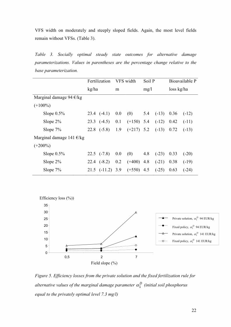
Figure 5. Efficiency losses from the private solution and the fixed fertilization rule for

alternative values of the marginal damage parameter 1

Dα (initial soil phosphorus

equal to the privately optimal level 7.3 mg/l)

0

5

10

15

20

25

30

35

0,5 2 7

Field slope (%)

Fixed policy, 1αD 94 EUR/kg

Private solution, 1αD 141 EUR/kg

Fixed policy, 1αD 141 EUR/kg

Private solution, 1αD 94 EUR/kg

Efficiency loss (%))

23

For both alternative damage parameterizations, the fixed fertilizer application rule

outperforms the privately optimal outcome in terms of social welfare, with an

efficiency loss of less than 6% even for the steeply sloped parcel (Figure 5). Here, the

need for depletion is relatively small compared to the high initial phosphorus reserve

discussed in the previous section: The difference between the socially and privately

optimal steady state phosphorus levels is on the order of 2-3 mg/l. The result still

holds for the alternative damage parameterizations that the privately optimal path

produces higher welfare than the fixed fertilization rate when the initial soil

phosphorus is at a high level.

6 Policy implications

The results show that efficient policies to reduce phosphorus loading from agricultural

land should adjust fertilization application rates in response to changes in the soil

phosphorus level, in particular where the initial soil phosphorus stock is notably above

the target level. The empirical illustration shows that adjustments can be significant:

the optimal fertilizer rate ranged from 0 to almost 70 kg/ha/year for an empirically

reasonable range of soil phosphorus levels. The results also indicate that erosion

control policy should focus on land most susceptible to erosion and is not very

sensitive to changes in soil phosphorus level. A similar result was discussed by Iho

(2007) who, however, considered only steady state results. The modest interlinkage

between soil phosphorus level and erosion control is somewhat surprising, given that

the bioavailability of particulate phosphorus in the empirical model considered here,

and hence the environmental damage from erosion, increases with soil phosphorus.

The sensitivity of optimal fertilization rate to soil phosphorus level indicates that

matching fertilizer application with the existing soil phosphorus stock has an

important impact on welfare. We quantified this impact by comparing the welfare

generated by the socially optimal path to that generated by a fixed fertilization rule

and the privately optimal path. When the initial soil phosphorus level is very high –

significantly above the privately optimal steady state – adjusting phosphorus

application based on the soil phosphorus level, even without accounting for

environmental damage from phosphorus loading, produces notable efficiency gains

relative to following a fixed application rate. If, for example, land previously in sugar

24

beet production is allocated to grains, phosphorus reserves are likely to be markedly

above the level optimal for grains. Our empirical example suggests that as long as a

private farmer knows the role of phosphorus in crop production and how the soil

phosphorus reserves develop in response to phosphorus fertilization, the social

welfare produced by the privately optimal depletion path can be very close to that of

the socially optimal path. In our example, where the private farmer employed

precision phosphorus management, the efficiency loss from no policy intervention

was less than 5%. The efficiency loss from a simple fixed policy rule was markedly

higher, close to 20%. These findings emphasize the importance of improved precision

in phosphorus application as a means to reduce phosphorus loading from agricultural

land. Furthermore, information provision through farmer education and training may

offer a means to manage phosphorus loading at a relatively low cost.

7 Discussion

This paper presents a bioeconomic model for efficient phosphorus management in

agriculture. The model tailors phosphorus application to existing soil phosphorus

stock and accounts for environmental damage from phosphorus loading. It considers

depletion of soil phosphorus reserves and erosion control through vegetative filter

strips as measures to reduce phosphorus loading. The proposed dynamic programming

approach and numerical solution method make it possible to incorporate state-of-the-

art descriptions of crop production and agricultural phosphorus loading into the

dynamic optimization framework. The model provides guidelines for the timing and

intensity of phosphorus application and erosion control in different conditions. We

calibrated the model for barley production in southern Finland in order to provide an

empirical illustration of the importance of precision phosphorus management in

reducing agricultural phosphorus loading.

The empirical results indicate that optimal dynamic adjustments in phosphorus

application rates can have an important impact on social welfare. In fact, when

starting from initially very high phosphorus levels, even a privately optimal solution

matching fertilization to the existing soil phosphorus stock outperformed a fixed

fertilization rule based on the socially optimal steady state. The results also confirm

that reducing agricultural phosphorus loading requires long-term efforts: for soils

25

initially very rich in phosphorus, phosphorus losses remain elevated for decades even

when fertilization is reduced markedly.

The analysis presented here focused on determining optimal dynamic policy rules for

agricultural phosphorus management. We considered a field parcel homogenous in

soil characteristics and assumed perfect information about the soil phosphorus level.

An important extension to this study would be to address the implications for

phosphorus management of spatial variability in soil characteristics, which entails

uncertainty about existing soil phosphorus. As pointed out by Lichtenberg (2002),

appropriate sampling can reduce such uncertainty or even eliminate it, but there have

been few studies investigating optimal sampling or testing strategies in an economic

context. Regulations and incentive mechanisms to correct the externality associated

with phosphorus loading were also not considered. An important focus for future

work would be to investigate regulatory policies such as taxes and subsidies, and, as

Xabadia et al. (2008) have done, to assess the gains from adjusting policies

dynamically in response to soil phosphorus levels and from targeting policies to areas

susceptible to erosion. While our analysis showed that tailoring fertilizer application

to the prevailing field conditions produces the highest welfare, policy makers need to

know whether the welfare gains suffice to offset the costs of investments in human

and physical capital and increased monitoring that such policies may entail. Khanna

and Zilberman (1997) provide a framework for studying the adoption of precision

technology that could be combined with our model of crop production and pollution

generation in order to design policies that would encourage more precise phosphorus

management. Extending the model to optimal dynamic control of phosphorus loading

from animal farms is also left for illumination by future research.

26

Acknowledgements

A part of this research was done while Marita Laukkanen was visiting the Department

of Agricultural and Resource Economics at the University of California, Berkeley,

and Laukkanen wishes to thank the department for its hospitality. Iho wishes to thank

the Finnish Cultural Foundation and the Kyösti Haataja Foundation for financial

support. A part of the research was done while Iho was working at the Department of

Economics and Management, University of Helsinki. The authors also thank Markku

Ollikainen, Petri Ekholm, Marko Lindroos, Eila Turtola and David Zilberman for

insightful comments. All remaining errors are the authors’ responsibility.

27

References

Bellman, R. 1957. Dynamic Programming. Princeton: Princeton University Press.

Ekholm, P. and Krogerus, K. 2003. “Determining Algal-Available Phosphorus of

Differing Origin: Routine Phosphorus Analyses versus Algal Assays.”

Hydrobiologia 492: 29-42.

Ekholm, P., Turtola, E. Grönroos, J., Seuri, P. and Ylivainio, K. 2005. “Phosphorus

Loss from Different Farming Systems Estimated from Soil Surface

Phosphorus Balance.” Agriculture, Ecosystems and Environment 110: 266-

278.

Eurostat (2009). Sugar beet: Number of farms and area by size of farm (UAA) and

size of sugar beet area. Retrieved May 26, 2009, from

http://nui.epp.eurostat.ec.europa.eu/nui/show.do?dataset=ef_lu_alsbeet&lang=

en.

Goetz, R-U. and Keusch, A. 2005. “Dynamic Efficiency of Soil Erosion and

Phosphorus Reduction Policies Combining Economic and Biophysical

Models.” Ecological Economics 52: 201-218.

Goetz, R-U. and Zilberman, D. 2000. “The Dynamics of Spatial Pollution: the Case of

Phosphorus Runoff from Agricultural Land.” Journal of Economic Dynamics

and Control. 24:143-163.

Gren, I-M. and Folmer, H. 2003. “Cooperation with Respect to Cleaning of an

International Water Body with Stochastic Environmental Damage: the Case of

the Baltic Sea.” Ecological Economics 47:33– 42

Helsinki Commission 2004. “The Fourth Baltic Sea Pollution Load Compilation.”

Helsinki: Baltic Sea Environment Proceedings 93.

Helin, J., Laukkanen, M., Koikkalainen, K. 2006. ”Abatement Costs for Agricultural

Nitrogen and Phosphorus Loads: a Case Study of Crop Farming in South-

Western Finland.” Agricultural and Food Science 15(4): 351-374.

Hooda, P., Truesdale, V., Edwards, A., Withers, P., Aitken, M., Miller, A. and

Rendell, A. 2001. “Manuring and Fertilization Effects on Phosphorus

Accumulation in Soils and Potential Environmental Implications.” Advances

in Environmental Research 5: 13–21.

Iho, A. 2007. Dynamically and Spatially Efficient Phosphorus Policies in Crop

Production. University of Helsinki, Department of Economics and

28

Management. Publications 43. Licentiate thesis. Available online:

http://www.mm.helsinki.fi/mmtal/abs/Pub43.pdf.

Khanna, M. and and Zilberman, D. 1997. “Incentives, Precision Technology and

Environmental Protection.”. Ecological Economics 23: 25-43.

Kennedy, J.O.S 1986. Dynamic Programming, Applications to Agriculture and

Natural Resources. Elsevier.

Lambert, D.M., Lowenber-DeBoer, J. and Malzer, G. 2007. “Managing Phosphorus

Soil Dynamics over Space and Time.” Agricultural Economics 37:43-53.

Lankoski, J., Ollikainen, M. and Uusitalo, P. 2006. ”No-till Technology: Benefits to

Farmers and the Environment? Theoretical Analysis and Application to

Finnish Agriculture.” European Review of Agricultural Economics 33(2): 193-

221.

Lichtenberg, E. 2002. Agriculture and Environment. In B. Gardner and G. Rausser

(eds.), Handbook of Agricultural Economics. Vol 2. North Holland,

Amsterdam, pp. 1249-1313.

Miranda, J.M. and Fackler, P.L. 2002. Applied Computational Economics and

Finance. Cambridge: MIT Press.

Myyrä, S., Pietola, K. and Yli-Halla, M. 2007. ”Exploring Long-Term land

Improvements under Land Tenure Insecurity.” Agricultural Systems 92:63-75.

Palva, R. 2003. “Vegetative Filter Strip Maintenance.” Agricultural Bulletin 4/2003

(555). Work Efficiency Institute, Helsinki, Finland (in Finnish).

Pentti, S. and Laaksonen, K. “Machinery Costs and Statistical Contractor Prices.

Agricultural Bulletin 4/2005 (577).” Work Efficiency Institute, Helsinki,

Finland (in Finnish).

Puustinen, M., Merilä, E., Palko, J. and Seuna, P. 1994. ”Drainage Status, Cultivation

Practices and Factors Affecting Nutrient Loading from Finnish Fields.”

Publications of the Water and Environment Agency, Series A (198). Finnish

Environment Institute, Helsinki, Finland (in Finnish).

Redfield, A.C., Ketchum, B.H. and Richards F.A. 1963. “The Influence of Organisms

on the Composition of Seawater.” In M.N. Hill, ed. The Sea, vol. 2. New

York: Wiley.

Saarela, I., Järvi, A., Hakkola, H. and Rinne, K. 1995. ”Field Trials on Fertilization

1977-1994.” Agrifood Research Finland Bulletin No. 16. Agrifood Research

Finland, Jokioinen, Finland (in Finnish).

29

Sharpley, A.N. 1993. “Assessing Phosphorus Bioavailability in Agricultural Soils and

Runoff.” Fertilizer Research 36:259-272.

Sharpley, A. N. and Rekolainen, S. 1997. “Phosphorus in Agriculture and

Environmental Implications.” In H. Tunney, O. T. Carton, P. C. Brookes, and

A. E. Johnson, eds. Phosphorus Losses from Soil to Water. Cambridge, UK:

CAB International, pp. 1–54.

Schnitkey, G., D. and Miranda, M., J. 1993. “The Impact of Pollution Controls on

Livestock-Crop Producers.” Journal of Agricultural and Resource Economics

18(1): 25-36.

Shortle, J.S. and Abler, D.G. 1999. “Agriculture and the Environment.” In J. van den

Bergh ed. Handbook of Environmental and Resource Economics.

Cheltenhamn: Edward Elgar, pp. 159-176.

Turtola, E. and Paajanen, A. 1995. “Influence of Improved Subsurface Drainage on

Phosphorus Losses and Nitrogen Leaching from a Heavy Clay Soil.”

Agricultural Water Management 28: 295-310.

Uusi-Kämppä, J. and Kilpinen, M. 2000. Mitigation of Nutrient Loss through

Vegatative Filter Strips. Agrifood Research Finland Bulletin 83. Agrifood

Research Finland, Jokioinen, Finland (in Finnish).

Uusitalo, R. and Jansson, H. 2002. “Dissolved Reactive Phosphorus in Runoff

Assessed by Soil Extraction with an Acetate Buffer.” Agricultural and Food

Science in Finland 11: 343-353.

Uusitalo, R., Turtola, E., Puustinen, M., Paasonen-Kivekäs, M. and Uusi-Kämppä, J.

2003. “Contribution of Particulate Phosphorus to Runoff Phosphorus

Bioavailability.” Journal of Environmental Quality 32: 2007-2016.

Uusitalo, R., Ekholm, P., Turtola, E., Pitkänen, H., Lehtonen, H., Granlund, K., Bäck,

S., Puustinen, M., Räike, A., Lehtoranta, J., Rekolainen, S., Walls, M. and

Kauppila, P. 2007. ”Agriculture and Baltic Sea Eutrophication.” Agriculture

and Food Production 96, Agrifood Research Finland. Jokioinen, Finland (in

Finnish).

Wischmeier, W.H. and Smith, D.D. 1978. “Predicting Rainfall Erosion Losses.”

Washington D.C: U.S. Department of Agriculture, Agricultural Handbook

537.

30

Xabadia, A., Goetz, R. and Zilberman, D. 2008. “The Gains from Differentiated

Policies to Control Stock Pollution when Producers Are Heterogenous.”

American Journal of Agricultural Economics 90(4): 1059-1073.

Yli-Halla, M., Hartikainen, H., Ekholm, P., Turtola, E., Puustinen, M. and Kallio, K.

1995. ”Assessment of Soluble Phosphorus Load in the Surface Runoff by Soil

Analyses.” Agriculture, Ecosystems and Environment 56: 53–62.

ISSN 1795-5300

MTT Discussion Papers 4 • 2009MTT Discussion Papers 4 • 2009

Dynamically Optimal Phosphorus Management

and Agricultural Water Protection

Antti Iho & Marita Laukkanen