dynamic simulation of mitral valve using the immersed boundary method
DESCRIPTION
Dynamic simulation of mitral valve using the Immersed boundary method. Dr. Xiao Yu Luo Department of Mathematics University of Glasgow Glasgow, G12 8QW UK. Acknowledgement. Dr. Paul Watton, Mr. Min Yin Dept. of Mathematics, University of Glasgow. Professor Wheatley, Dr. G. Bernacca - PowerPoint PPT PresentationTRANSCRIPT
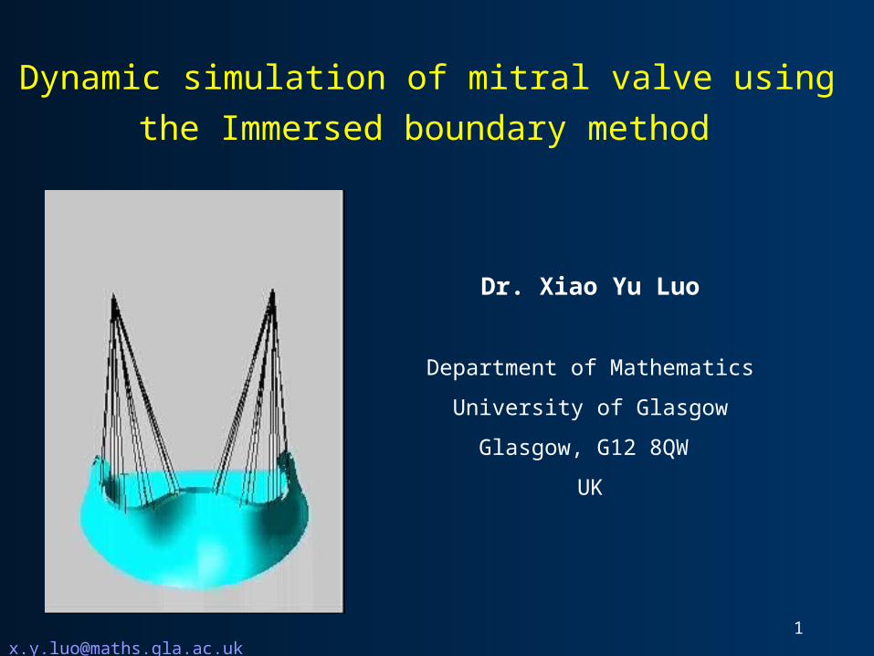
Dynamic simulation of mitral valve using
the Immersed boundary method
Dr. Xiao Yu Luo
Department of Mathematics
University of Glasgow
Glasgow, G12 8QW
UK

Acknowledgement
Dr. Paul Watton, Mr. Min Yin
Dept. of Mathematics, University of Glasgow.
Professor Wheatley, Dr. G. Bernacca
Dept of Cardiac Surgery, University of Glasgow, Glasgow, UK
Professor Xiaodong Wang
Department of Mathematical Sciences, New Jersey Institute of Technology.

• MV: two leaflets, anterior leaflet (larger), and posterior leaflet (smaller).
• Chordae run from valve leaflets to papillary muscles at the base of ventricle.
Anatomy of a mitral valve (MV)
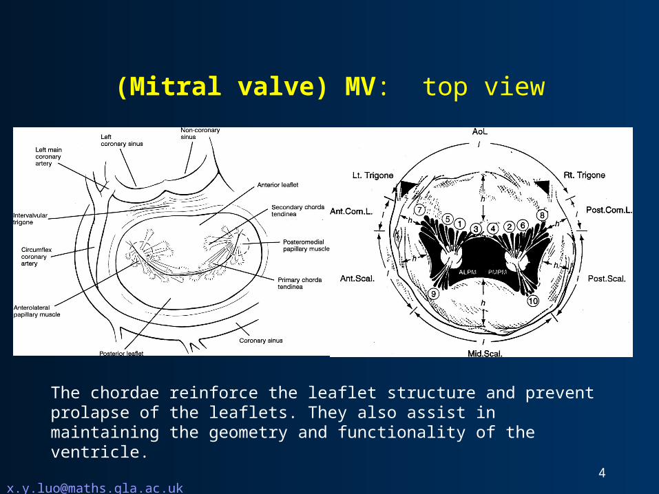
(Mitral valve) MV: top view
The chordae reinforce the leaflet structure and prevent prolapse of the leaflets. They also assist in maintaining the geometry and functionality of the ventricle.
MV diseases
• Typical diseases of MV: Mitral stenosis & mitral regurgitation.
• MV needs to be repaired or replaced when damaged.
• Two types of valve replacements: mechanical and bioprosthetic valves.
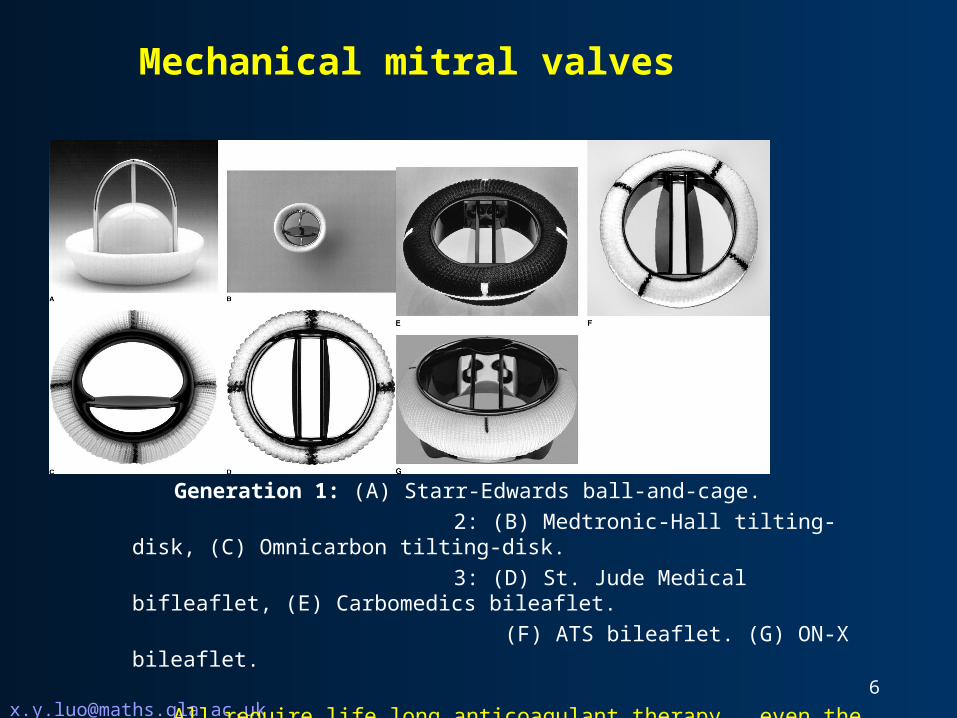
Mechanical mitral valves
Generation 1: (A) Starr-Edwards ball-and-cage.
2: (B) Medtronic-Hall tilting-disk, (C) Omnicarbon tilting-disk.
3: (D) St. Jude Medical bifleaflet, (E) Carbomedics bileaflet.
(F) ATS bileaflet. (G) ON-X bileaflet.
All require life long anticoagulant therapy, even the best designs have risks of
hemorrhage related to anticoagulant therapy and thromboembolism

Bioprosthetic mitral valves.
Generation 1: (A) Hancock II porcine heterograft,
2: (B) Carpentier-Edwards standard porcine heterograft, (C) Mosaic porcine
heterograft.
3: (D) Carpentier-Edwards pericardial bovine heterograft.
20% failing with 10 years. Rate of deterioation accelerates for young patients.

Use of aortic valve design, and put in reversed configuration:
Potential of changing the vortex structure in the flow inside the ventricle.
Have no chordae attached:
Potential of changing the ventricle wall mechanics, and causes prolapse.
Clinical observation: The durability of porcine valves is less with mitral bioprostheses than with aortic bioprostheses.
Current designs offer no ideal substitutes
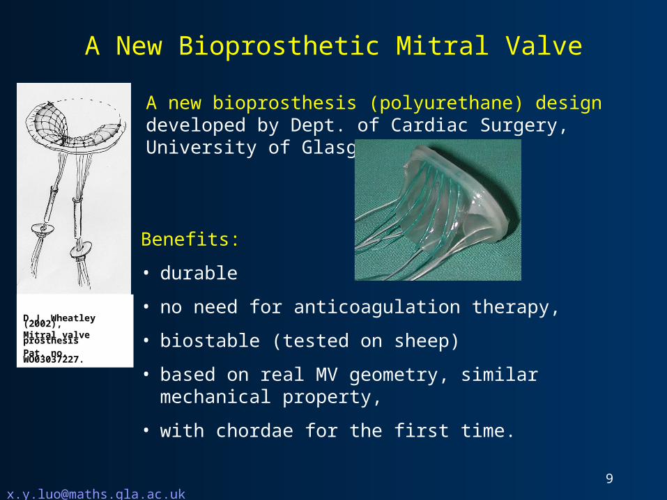
A New Bioprosthetic Mitral Valve
D.J. Wheatley (2002), Mitral valve prosthesis
Pat. no. WO03037227.
A new bioprosthesis (polyurethane) design developed by Dept. of Cardiac Surgery, University of Glasgow
Benefits:
• durable
• no need for anticoagulation therapy,
• biostable (tested on sheep)
• based on real MV geometry, similar mechanical property,
• with chordae for the first time.
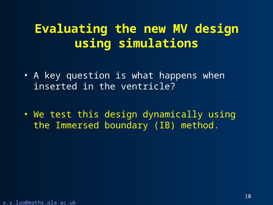
Evaluating the new MV design using simulations
• A key question is what happens when inserted in the ventricle?
• We test this design dynamically using the Immersed boundary (IB) method.

Fluid:
, , , ,
1, 0
Rei
i j j i i jj j j
uu u p u u
tf
where solid behaves like fibres immersed in the fluid. It imposes force f on the fluid, and is moved by the fluid.
( , ) ( ),X
F r t T Ts s
r: fibre point coordinates, T: tension
x: fluid coordinates,
ss
X(r,t)
Immersed Boundary (IB) Method
( , )( , ) ( ( , )) ,X
r t X r tt
u x t x dx
( , ) ( ( , )) ,F r t X r t dsf x
Solid:
Interactions:
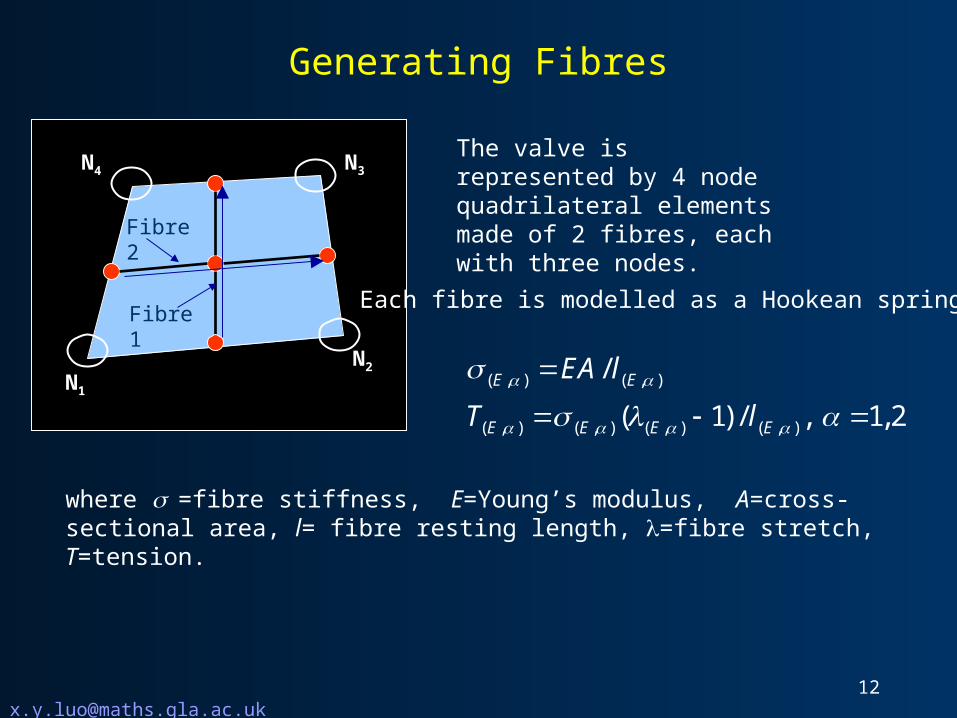
Generating Fibres
The valve is represented by 4 node quadrilateral elements made of 2 fibres, each with three nodes.
N1
N2
N3N4
Fibre 1
Fibre 2
( , ) ( , )
( , ) ( , ) ( , ) ( , )
/
( 1) / , 1, 2
E E
E E E E
EA l
T l
where =fibre stiffness, E=Young’s modulus, A=cross-sectional area, l= fibre resting length, =fibre stretch, T=tension.
Each fibre is modelled as a Hookean spring:

where, u(r,t) is the velocity of the fibres.
Note if two nodal points on two different fibres have identical spatial positions at t=0, then this will be true for all successive times. Tethering fibres with a great stiffness, make use of this fact to enforce boundary conditions.
The tethering fibres
( , )) ( ( , ))
)
)( ,
( ,
u x t x dxX
r
u r
t X r tt
t

Smooth approximation of Delta function
3
1( ) ( ) ( )h
x y z
h h h h
h: grid size
Fluid: on a fixed Eulerian grid, Solid: network of fibres on a Lagrangian mesh.

Solving Fluid equations with FFT
• The matrix equation of the discretized Navier-Stokes equations are
Kun+1=F(un)
where un is the solution vector at the nth time step.
• This is linear in un+1, thus can be solved using the Fast Fourier Transform method (recall that the Eulerian grid is uniform).
• In other words, we now need to have periodic boundary conditions.
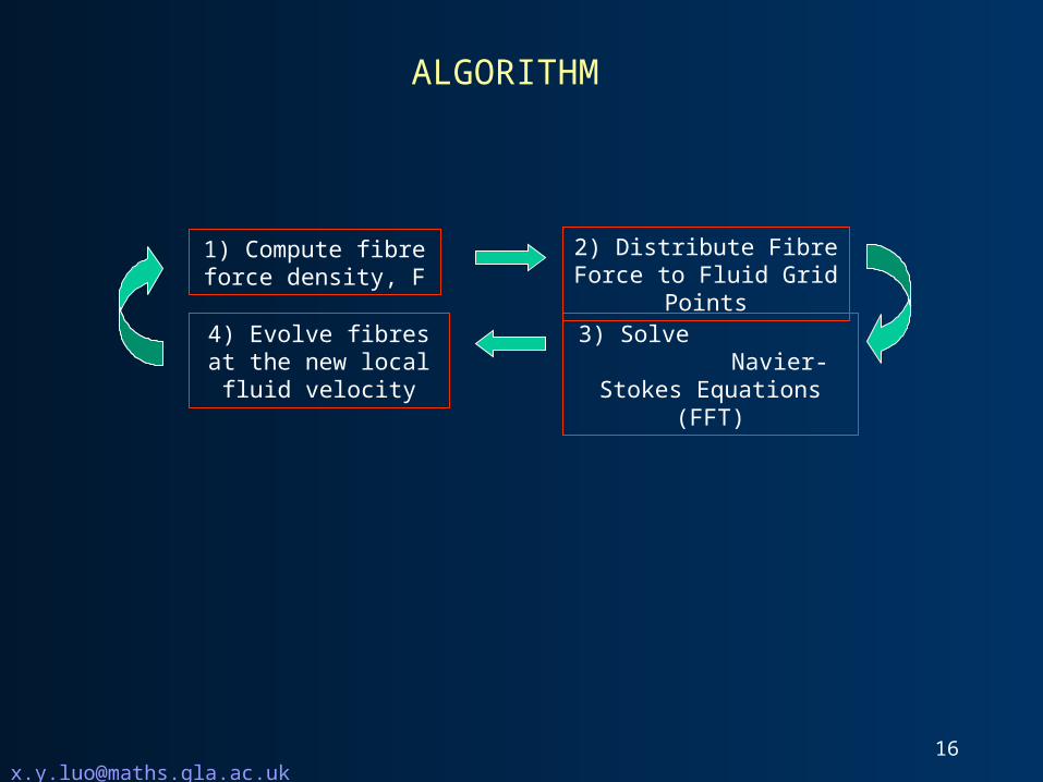
ALGORITHM
1) Compute fibre force density, F
2) Distribute Fibre Force to Fluid Grid
Points3) Solve
Navier-Stokes Equations (FFT)
4) Evolve fibres at the new local fluid
velocity
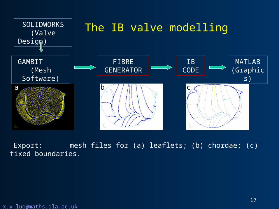
Export: mesh files for (a) leaflets; (b) chordae; (c) fixed boundaries.
GAMBIT (Mesh Software)
FIBRE GENERATOR
IB CODE
a cb
MATLAB (Graphics)
SOLIDWORKS (Valve Design)
The IB valve modelling
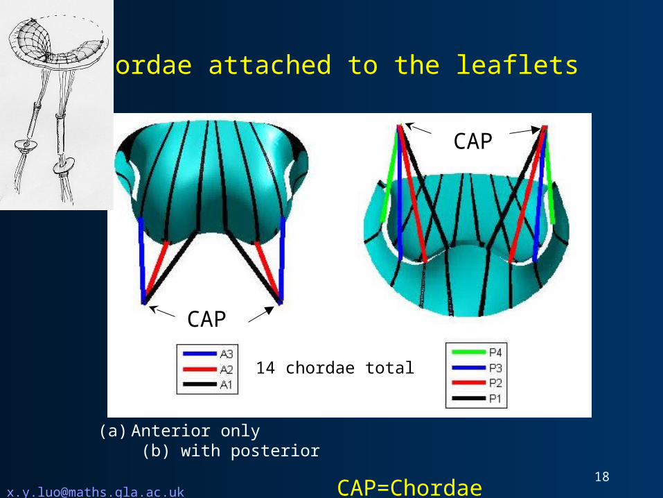
Chordae attached to the leaflets
(a) Anterior only (b) with posterior
CAP=Chordae Attachment Points
CAP
CAP
14 chordae total

The IB Model
• Cylindrical Tube: Length 16cm Diameter 5.6cm.
• Experimentally determined periodic velocity profile prescribed.
• Viscosity: 0.01g/m.s Density: 1g/cm3
• Submerged within a fluid mesh: size 64x64x64
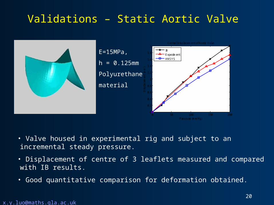
Validations – Static Aortic Valve
E=15MPa,
h = 0.125mm
Polyurethane
material
• Valve housed in experimental rig and subject to an incremental steady pressure.
• Displacement of centre of 3 leaflets measured and compared with IB results.
• Good quantitative comparison for deformation obtained.
0 50 100 150 2000
0.2
0.4
0.6
0.8
1
1.2
1.4
1.6
1.8
2
Pressure (mmHg)
Dis
plac
emen
t (m
m)
Central Displacement of Aortic Valve
IB
Experiment
ANSYS
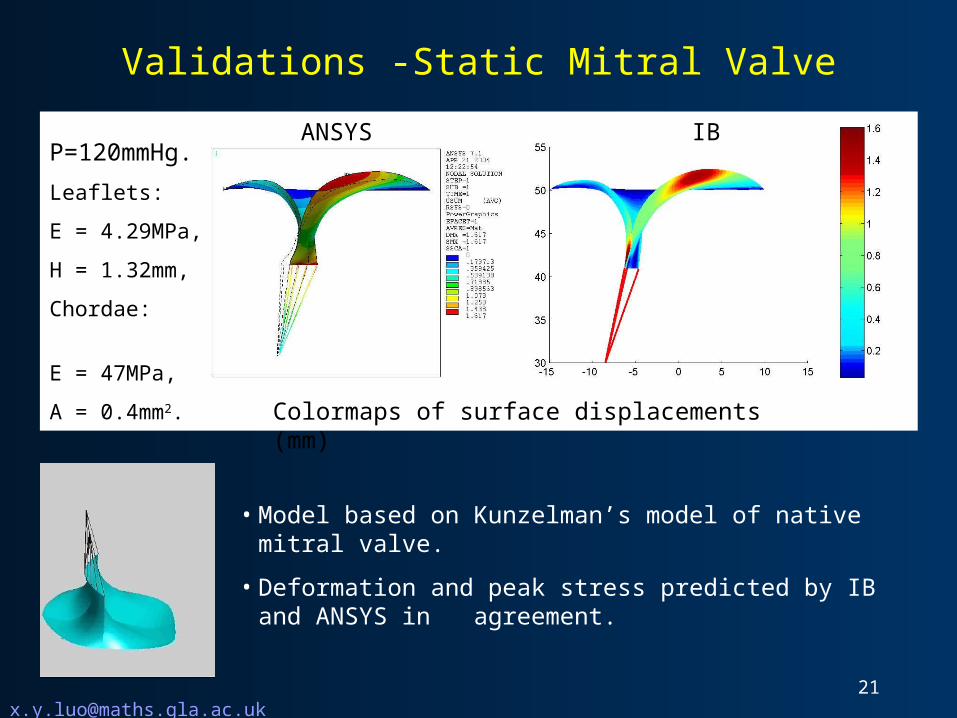
Validations -Static Mitral Valve
• Model based on Kunzelman’s model of native mitral valve.
• Deformation and peak stress predicted by IB and ANSYS in agreement.
P=120mmHg.
Leaflets:
E = 4.29MPa,
H = 1.32mm,
Chordae:
E = 47MPa,
A = 0.4mm2.
ANSYS IB
Colormaps of surface displacements (mm)

IB versus ANSYS
• IB is much better with thin structures. Ansys has “locking” phenomenon, hence a thicker shell has to be used (increasing thickness by 3-4 times, while reducing Young’s modulus by the same scale).
• IB is fast• IB is designed for dynamic modelling. Ansys is
not.
• Current IB has no bending.• Current IB is not so good with contact problems.

Validations: Dynamic MV with fixed CAP
Polyurethane leaflets: E = 5MPa, h = 0.125mm Chordae: E = 30MPa, Area = 0.4mm2
• Computation model of valve behaves too flexibly.
• Unrealistic crimping of leaflets occurs.
• IB unable to model bending effects.
Experimentally determined flow profile prescribed.
NOTE: Chordae are in leaflet surface in computational model but not visually represented.
Time (s)
Flo
w R
ate
(ml/s
)
0 0.1 0.2 0.3 0.4 0.5 0.6 0.7 -200
-100
0
100
200
300
Time (s)
Flo
w R
ate
(m
l/s)
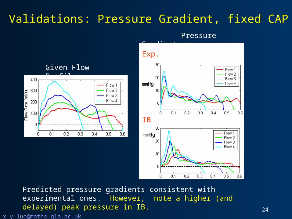
Validations: Pressure Gradient, fixed CAP
Given Flow Profiles
Pressure Gradients
mmHg
Predicted pressure gradients consistent with experimental ones. However, note a higher (and delayed) peak pressure in IB.
Exp.
IB
mmHg
mmHg

• Analyse Human MRI data with CMRTOOLS - software package for analysing Cardiovascular Magnetic Resonance (CMR) images (Imperial College www.cmrtools.com)
• Determine dynamic geometry of ventricle and papillary muscle axes.
• Intersection of data enables papillary muscle regions of ventricle to be identified
Physiological Chordae Attachemnt Points (CAP) motions

Track Mitral Annulus
DIASTOLE SYSTOLE
• Software package Slice-o-Matic used to analyse MRI data.
• Tracks motion of Mitral Annulus through 2 planes (32 Time Slices of Data)
• Note relative displacement of mitral annulus plane to apex of ventricle is obtained.
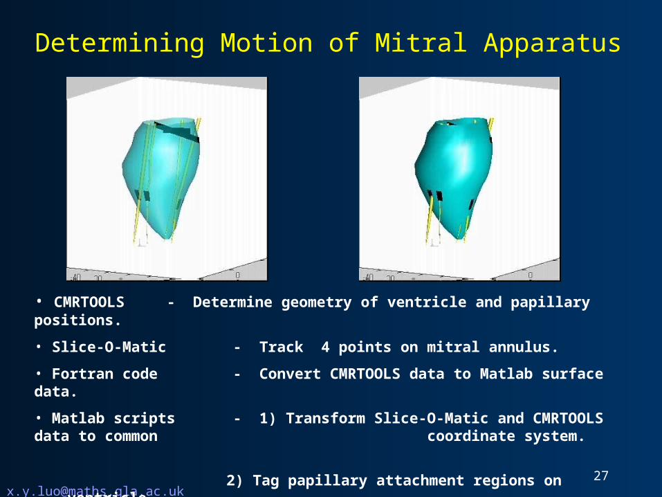
Determining Motion of Mitral Apparatus
• CMRTOOLS - Determine geometry of ventricle and papillary positions.
• Slice-O-Matic - Track 4 points on mitral annulus.
• Fortran code - Convert CMRTOOLS data to Matlab surface data.
• Matlab scripts - 1) Transform Slice-O-Matic and CMRTOOLS data to common coordinate system.
2) Tag papillary attachment regions on ventricle.
3) Determine relative motion of mitral apparatus.
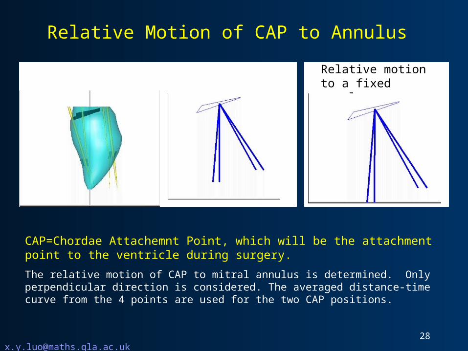
Relative motion to a fixed annulus
Relative Motion of CAP to Annulus
CAP=Chordae Attachemnt Point, which will be the attachment point to the ventricle during surgery.
The relative motion of CAP to mitral annulus is determined. Only perpendicular direction is considered. The averaged distance-time curve from the 4 points are used for the two CAP positions.
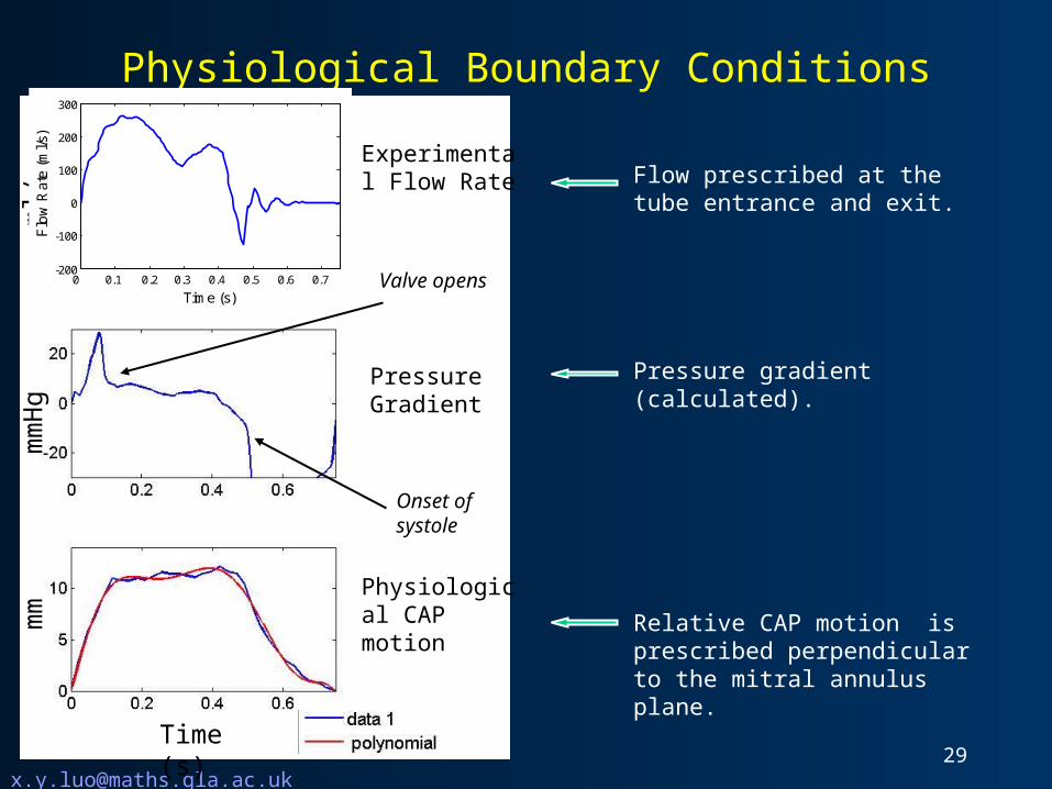
Flow prescribed at the tube entrance and exit.
Pressure gradient (calculated).
Relative CAP motion is prescribed perpendicular to the mitral annulus plane.
Physiological Boundary Conditions
Time (s)
ml/s
mm
Hg
mm
Experimental Flow Rate
Pressure Gradient
Physiological CAP motion
Valve opens
Onset of systole
0 0.1 0.2 0.3 0.4 0.5 0.6 0.7 -200
-100
0
100
200
300
Time (s)
Flo
w R
ate
(m
l/s)

Pressure Gradients
Opening pressure gradient reduces with CAP motion.
0 0.2 0.2 0.3 0.4 0.5 0.6 0.7-60
-40
-20
0
20
40
time (s)
Pre
ssu
re (
mm
Hg
)Fixed CAP
CAP Motion

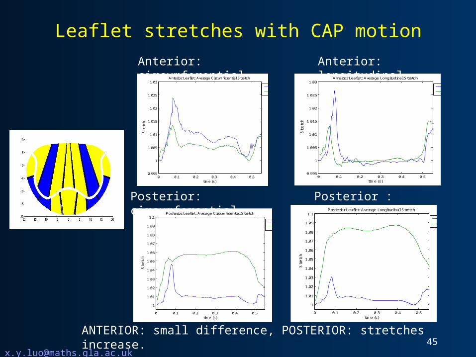
Leaflet stretches with CAP motion
ANTERIOR: small difference, POSTERIOR: stretches increase.
Anterior: circumferential
Posterior: circumferential
Anterior: longitudinal
Posterior : longitudinal
0 0.1 0.2 0.3 0.4 0.5 0.6 0.70.995
1
1.005
1.01
1.015
1.02
1.025
1.03
time (s)
Str
etc
h
Anterior Leaflet: Average Circumferential Stretch
Fixed CAP
CAP Motion
0 0.1 0.2 0.3 0.4 0.5 0.6 0.70.995
1
1.005
1.01
1.015
1.02
1.025
1.03
time (s)
Str
etc
h
Anterior Leaflet: Average Longitudinal Stretch
Fixed CAP
CAP Motion
0 0.1 0.2 0.3 0.4 0.5 0.6 0.7
1
1.02
1.04
1.06
1.08
1.1
time (s)
Str
etc
h
Posterior Leaflet: Average Circumferential Stretch
Fixed CAP
CAP Motion
0 0.1 0.2 0.3 0.4 0.5 0.6 0.7
1
1.02
1.04
1.06
1.08
1.1
time (s)
Str
etch
Posterior Leaflet: Average Longitudinal Stretch
Fixed CAP
CAP Motion
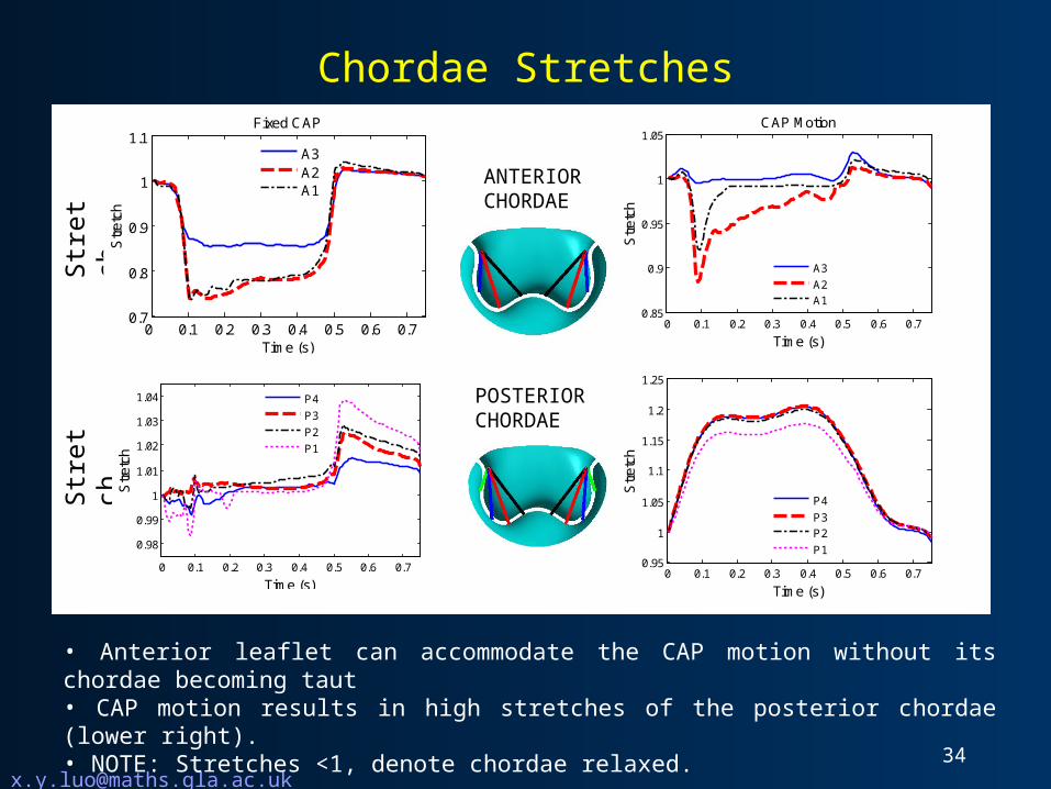
• Anterior leaflet can accommodate the CAP motion without its chordae becoming taut• CAP motion results in high stretches of the posterior chordae (lower right).• NOTE: Stretches <1, denote chordae relaxed.
Chordae StretchesS
tret
chS
tret
ch
NoANTERIOR CHORDAE
POSTERIOR CHORDAE
0 0.1 0.2 0.3 0.4 0.5 0.6 0.70.7
0.8
0.9
1
1.1
Time (s)
Str
etc
hFixed CAP
A3A2A1
0 0.1 0.2 0.3 0.4 0.5 0.6 0.70.85
0.9
0.95
1
1.05
Time (s)
Str
etc
h
CAP Motion
A3
A2A1
0 0.1 0.2 0.3 0.4 0.5 0.6 0.7
0.98
0.99
1
1.01
1.02
1.03
1.04
Time (s)
Str
etc
h
P4
P3
P2
P1
0 0.1 0.2 0.3 0.4 0.5 0.6 0.70.95
1
1.05
1.1
1.15
1.2
1.25
Time (s)
Str
etc
h
P4
P3P2
P1

• Anterior leaflet can accommodate CAP motion.
• Posterior leaflet subject to significantly higher stretches detrimental effect on the long-term durability of the valve.
Up to 20% strain increase due to papillary motion
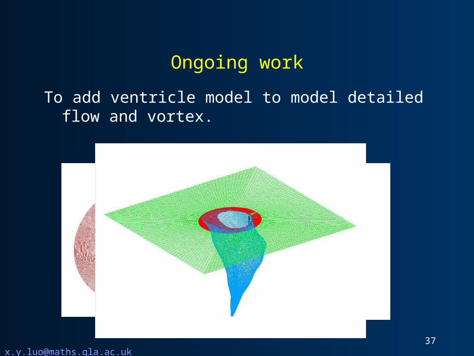

Ongoing work
Improvements for IB code:
• Developing a better solid model with bending stiffness.
• Use adaptive mesh to get rid of sticking effects when opening.
• Better boundary conditions.

Summary Dynamic analysis for a mitral valve with chordae attachment points
(CAP) moving with ventricle is carried out with a IB code. Results show that:
• CAP motion assists the opening of the valve (lower opening pressure gradients).
• Current design: posterior is over-stretched.
Recommendation for design improvements:
• Modify geometry to allow a greater movement of the posterior leaflet.
• Modify stiffness of posterior chordae: low modulus external chordae that can accommodate high stretches, and high modulus internal leaflet chordae, which resist deformation
• Design a stiffer posterior leaflet which does not require chordae.

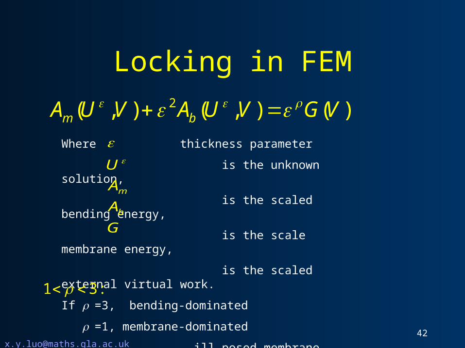
Locking in FEM2( , ) ( , ) ( )m bA U V A U V G V
Where thickness parameter
is the unknown solution,
is the scaled bending energy,
is the scale membrane energy,
is the scaled external virtual work.
If =3, bending-dominated
=1, membrane-dominated
ill-posed membrane problem
m
b
U
A
A
G
1 3:
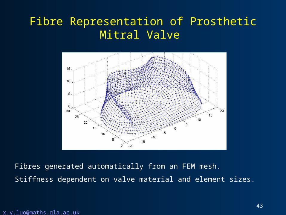
Fibre Representation of Prosthetic Mitral Valve
Fibres generated automatically from an FEM mesh.
Stiffness dependent on valve material and element sizes.
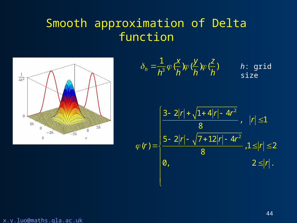
Smooth approximation of Delta function
3
1( ) ( ) ( )h
x y z
h h h h
2
2
3 2 1 4 4, 1
8
5 2 7 12 4( ) ,1 2
80, 2 .
r r rr
r r rr r
r
h: grid size
Leaflet stretches with CAP motion
ANTERIOR: small difference, POSTERIOR: stretches increase.
Anterior: circumferential
Posterior: circumferential
Anterior: longitudinal
Posterior : longitudinal
0 0.1 0.2 0.3 0.4 0.50.995
1
1.005
1.01
1.015
1.02
1.025
1.03
time (s)
Str
etc
h
Anterior Leaflet: Average Circumferential Stretch
Fixed CAP
CAP Motion
0 0.1 0.2 0.3 0.4 0.50.995
1
1.005
1.01
1.015
1.02
1.025
1.03
time (s)
Str
etc
h
Anterior Leaflet: Average Longitudinal Stretch
Fixed CAP
CAP Motion
0 0.1 0.2 0.3 0.4 0.5
1
1.01
1.02
1.03
1.04
1.05
1.06
1.07
1.08
1.09
1.1
time (s)
Str
etc
h
Posterior Leaflet: Average Circumferential Stretch
Fixed CAP
CAP Motion
0 0.1 0.2 0.3 0.4 0.5
1
1.01
1.02
1.03
1.04
1.05
1.06
1.07
1.08
1.09
1.1
time (s)
Str
etc
h
Posterior Leaflet: Average Longitudinal Stretch
Fixed CAP
CAP Motion