Facolta di IngegneriaDipartimento di Ingegneria Meccanica

Laurea Triennale in Ingegneria Meccanica

ESTIMATION OF THE IMMERSEDBOUNDARY TECHNIQUE FORINDUSTRIAL FLUID DYNAMIC

SIMULATIONS

Relatore:Prof. Ing. Roberto Verzicco

Candidato:Paolo Marafini

Triennio accademico 2009-2012

Abstract

The purpose of this work is to corroborate a new computational fluid dynamicssoftware produced by Karalit CFD.This program aims to provide reliable results for industrial applications withCFD, overcoming limitations that other codes have in front of complex geome-tries.The Immersed Boundary (IB) technique can satisfy the previous requests; thismethod adds to the Navier-Stokes equations a body-force f and maintains aCartesian computational domain.Two and three dimensional cases were analyzed with this method, the flow con-ditions were: steady flow or buoyancy-induced flow.Several three-dimensional examples of flow over a sphere for some Reynoldsnumbers were simulated and then compared with experimental results.In order to show the potential of Karalit CFD, in this paper, there are appli-cations that present significant difficulties for the traditional methods: so, thesoftware has been used with the same ease and satisfaction for objects with verycomplex geometry.

Abstract

Il presente lavoro e nato con l’intento di validare un nuovo software di fluidodi-namica computazionale prodotto dall’azienda Karalit.Il programma in questione mira a fornire alle industrie risultati attendibili nellaCFD, superando i limiti che i programmi precedentemente impiegati riscontra-vano di fronte a oggetti con geometrie complesse.Il metodo usato per fare cio e il metodo dei contorni immersi, il quale intervienenelle equazioni di Navier-Stokes aggiungendo un termine di forza di volume fmantenendo pero un dominio di calcolo basato su griglie cartesiane.Sono stati analizzati con questo metodo casi in due e tre dimensioni, sia incondizioni di moto del fluido stazionario sia con moto dovuto a gradienti ditemperatura.In particolare, per il caso 3D, si sono svolte piu simulazioni, variando solo ilnumero di Reynolds, riguardanti il flusso intorno ad una sfera, e si sono poiconfrontati i risultati con dati di letteratura.Per mostrare ulteriormente le potenzialita di Karalit CFD, si e pensato di stu-diare anche casi che, contrariamente alla sfera immersa in un fluido, presentanodifficolta ingenti di analisi con i metodi tradizionali: ebbene, la stessa facilita diapplicazione del programma si e potuta riscontrare con soddisfazione anche peroggetti a geometria molto complessa.

1

1 Karalit CFD

In the past the Immersed Boundary method was considered a mere researchtool, but now thanks to its “simplicity without compromise” is also used forindustrial applications.In this context the Karalit’s software has been created and implemented, thanksto cooperation between the Karalit CFD and the University of Rome “Tor Ver-gata” it has been possible to perform independent testing validation.This thesis was developed in three phases:

1. The simulation of several two-dimensional cases with the integration ofequations on structured grids, since the code used only this type of gridsin the early stages.

2. The use of the software to reproduce laboratory experiments followingthe possibility of using unstructured grids, and compare the simulationresults with the data available in the literature; in this way it was possibleto validate the data obtained by computational fluid dynamics.

3. The use of Karalit to simulate applications that present significant diffi-culties for the traditional methods, to emphasize Karalit’s versatility andspeed of use.

1.1 Karalit CFD Introduction

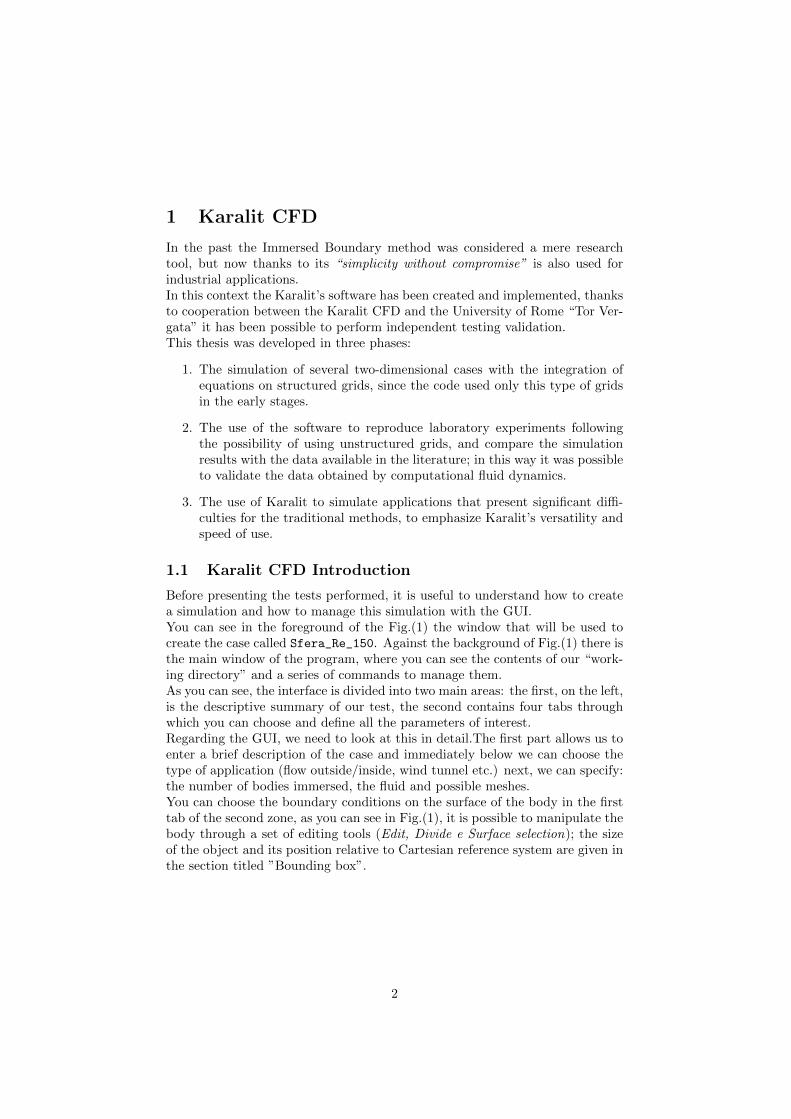
Before presenting the tests performed, it is useful to understand how to createa simulation and how to manage this simulation with the GUI.You can see in the foreground of the Fig.(1) the window that will be used tocreate the case called Sfera_Re_150. Against the background of Fig.(1) there isthe main window of the program, where you can see the contents of our “work-ing directory” and a series of commands to manage them.As you can see, the interface is divided into two main areas: the first, on the left,is the descriptive summary of our test, the second contains four tabs throughwhich you can choose and define all the parameters of interest.Regarding the GUI, we need to look at this in detail.The first part allows us toenter a brief description of the case and immediately below we can choose thetype of application (flow outside/inside, wind tunnel etc.) next, we can specify:the number of bodies immersed, the fluid and possible meshes.You can choose the boundary conditions on the surface of the body in the firsttab of the second zone, as you can see in Fig.(1), it is possible to manipulate thebody through a set of editing tools (Edit, Divide e Surface selection); the sizeof the object and its position relative to Cartesian reference system are given inthe section titled ”Bounding box”.

2

Figure 1: User interface.

2 The flow past a sphere at varying Reynoldsnumbers

For the validation of Karalit CFD has been relied on this kind of simulationssince for this problem have been made many experiments and therefore thereare many laboratory data. All the simulations were made with the followingassumptions:

1. Steady axisymmetric flow 5 < Re < 200

2. Incompressible fluid

3. Characteristics of the simulations

• Density ρ = 1000 Kgm3

• Components of the velocity vector Vx = 2, 225 10−4 ms , Vy = Vz = 0

• Diameter of the sphere D = 1m

• Pressure p = 101325 Pa

• Temperature T = 228.15 K

• CFL = 100

• Maximum number of iterations equal to 500

• Monitoring x-momentum residual, stop when convergence reaches 10−4

The viscosity of the fluid µ has been changed in order to obtain the variationof the Reynolds number. The sphere was positioned in the center of a compu-tational domain, which is of cubic shape and twenty times larger Fig.(2).

The characteristics of the grid are:

3

Figure 2: Computational domain.

• Initial size of the grid to the extreme of the domain equal to the charac-teristic size of the sphere D;

• number of layers equal to 10;

• number of refinement equal to 5, so the minimum size of the cell is d =0.03125

The integration was performed according to the method of Gauss-Seidel andusing the scheme 2nd order symmetric TVD.

4

2.1 Simulations

In this work, four simulations are shown and the Reynolds numbers selected are:Re = 50, Re = 100, Re = 150, Re = 200. The software has been validated bythe results obtained from these cases. The geometric characteristics consideredare shown in Fig.(3)

Figure 3: Flow at Re = 50.

As illustrated in Fig.(3), the flow is seen to separate from the surface of thesphere at an angle ϑs from the front stagnation point, it forms a closed sepa-ration bubble (length Ls) and a toroidal vortex centred at (xc, yc). The com-parison between the literature data and the simulation data has been done onthese parameters. In the Fig.s(3-7) are shown the results of simulation, whilein Tab.(1) are reported the number of total cells for each simulation.

Re number of cells50 194216100 265420150 614552200 614552

Table 1: Re and number of cells

5

Figure 4: Flow at Re = 50. Figure 5: Flow at Re = 100.

Figure 6: Flow at Re = 150. Figure 7: Flow at Re = 200.

2.2 Comparison between simulations and data from theliterature

In addition to the geometric characteristics in Sec.(2.1) was also considered thedrag coefficient CD.

CD =Fx

12 ρVx

2 S

S is defined as S = πD2

4The comparison result is shown in Fig.s(8-11).The Fig.(9) was considered significant because the data reported by Johnson

and Patel and the data obtained from Magnaudet differ between them of 11.5%,exceeded the threshold of Re = 150, while those obtained from Karalit CFDare placed approximately in the middle between the two: in fact these resultsdeviate by 5% from the results of Johnson and Patel and 6.9% from the resultsof Magnaudet.

6

Figure 8: ϑs. Figure 9: Lb.

Figure 10: (xc, yc). Figure 11: CD.

7

Conclusions

After analyzing the results of simulations made with Karalit, a selection of whichis shown in this paper, the software can be considered validated. In fact, thecomparison between the data obtained from the simulator and those found inthe literature have always shown a substantial agreement.The immersed boundary method proved to be excellent also in simulations thatwere performed on objects of very complex form, which would cause considerabledifficulties when faced following the traditional methods.Another important factor is the ease with which Karalit CFD can be usedthrough its interface, so the user should not program, in fact, the user will onlyhave to enter the parameters simulation will be based on and choose the settingprovided by the software which he considers best for his test.The immersed boundary method, in combination with KARALIT, can breakdown considerably the setup time, in fact the methods normally used wouldhave required also a month of preparation, instead with this software only takesa few seconds to switch to simulation.The conclusion that can be drawn is that the usability of the immersed boundarymethod through a GUI turned out to be an excellent alternative to methods thatare normally used in the simulations of industrial applications.

8

References

[1] Vieceli JA (1969), A method for including arbitrary external boundaries inthe MAC incompressible fluid computing technique, J.Comput. Phys.

[2] Vieceli JA (1971), A computing method for incompressible flows bounded bymoving walls, J. Comput. Phys.

[3] Peskin CS (1972), Flow patterns around heart valves: A digital computermethod for solving the equations of motion, PhD thesis, Physiology, AlbertEinstein College of Medicine.

[4] Peskin CS and McQueen DM (1989), A three-dimensional computationalmethod for blood flow in the heart: (I) immersed elastic fibers in a viscousincompressible fluid, J. Comput. Phys.

[5] McQueen DM and Peskin CS (1989), A three-dimensional computationalmethod for blood flow in the heart: (II) contractile fibers, J. Comput. Phys.

[6] Briscolini M and Santangelo P (1989), Development of the mask method forincompressible unsteady flows, J. Comput. Phys.

[7] Saiki EM and Biringen S (1996), Numerical simulation of a cylinder in uni-form flow: Application of a virtual boundary method, J. Comput. Phys.

[8] L. J. Fauci and A. L. Fogelson (1993), Truncated newton method and mod-eling of complex immersed elastic structures, Comm. Pure Appld. Math.

[9] L. J. Fauci and C. S. Peskin (1988), A computational model of acquaticanimal locomotion, J. Comp. Phys.

[10] R. Dillon, L. J. Fauci, and D. Gaver (1995), A microscale model of bacterialswimming, chemotaxis and substrate support, J. Theor. Biol.

[11] Goldstein D, Handler R, and Sirovich L (1993), Modeling no-slip flowboundary with an external force field, J. Comput. Phys.

[12] J. Mohd-Yusof (1997), Combined Immersed Boundaries/B-Splines Methodsfor Simulations of Flows in Complex Geometries, CTR Annual ResearchBriefs, NASA Ames/Stanford University.

[13] E. A. Fadlun, R. Verzicco, P. Orlandi, and J. Mohd-Yusof (2000), Com-bined Immersed-Boundary Finite-Difference Methods for Three-DimensionalComplex Flow Simulations, J. Comput. Phys.

[14] De Zeeuw D and Powell KG (1993), An adaptive Cartesian mesh methodfor the Euler equations, J. Comput. Phys.

[15] Pember RJ, Bell BJ, Colella P, Crutchfield WJ, and Welcome ML (1995),An adaptive Cartesian grid method for unsteady compressible flow in irreg-ular regions, J. Comput. Phys.

9

[16] D. Angeli, P. Levoni, G. S. Barozzi (2008), Numerical predictions for stablebuoyant regimes within a square cavity a heated horizontal cylinder, Inter-national Journal of Heat and Mass Transfer.

[17] T. A. Johnson, V. C. Patel (1999), Flow past a sphere up to a Reynoldsnumber of 300, Iowa Institute of Hydraulic Research and Department ofMechanical Engineering.

[18] R. Verzicco (2006), Appunti di Turbolenza, Universita degli studi di Roma“Tor Vergata” Dipartimento di Ingegneria Meccanica.

10