dynamic model for stock market risk evaluation kasimir kaliva and lasse koskinen insurance...
TRANSCRIPT
Dynamic Model for Stock Market Risk Evaluation
Kasimir Kaliva and Lasse Koskinen
Insurance Supervisory Authority
Finland

Goal: Stock Market Risk Modelling in Long Horizon
• Phenomenon: Stock market bubble
• Model should work from one quarter to several years– Prices should be mean reverting
• Fundament: Dividend / Price – ratio
• Explanatory factor: Inflation
• Usage: Risk Assessment and DFA

Background• Theory: Gordon growth model for dividend
Dynamics: Campbell et al, also near Wilkie– Dividend-price-ratio (P/D) time-varying,
stationary=>Mean reversion in stock pricesInflation expectation: Modigliani and Cohn (79)
• Statistical model: – Logistic Mixture Autoregression with
exogenous variable (Wong and Li (01))– Conditional (dynamic) on P/D -ratio

Data
• U.S. quarterly stock market (SP500) and inflation series; Log returns and dividens– Prices and dividends
• Period: 1959 –1994
• Structural breaks in dividend series and price/dividend –series in 1958 and 1995
• 1995- 2001 – share repurchases and growth strategies won popularity

Structural Break in Dividends in 1955
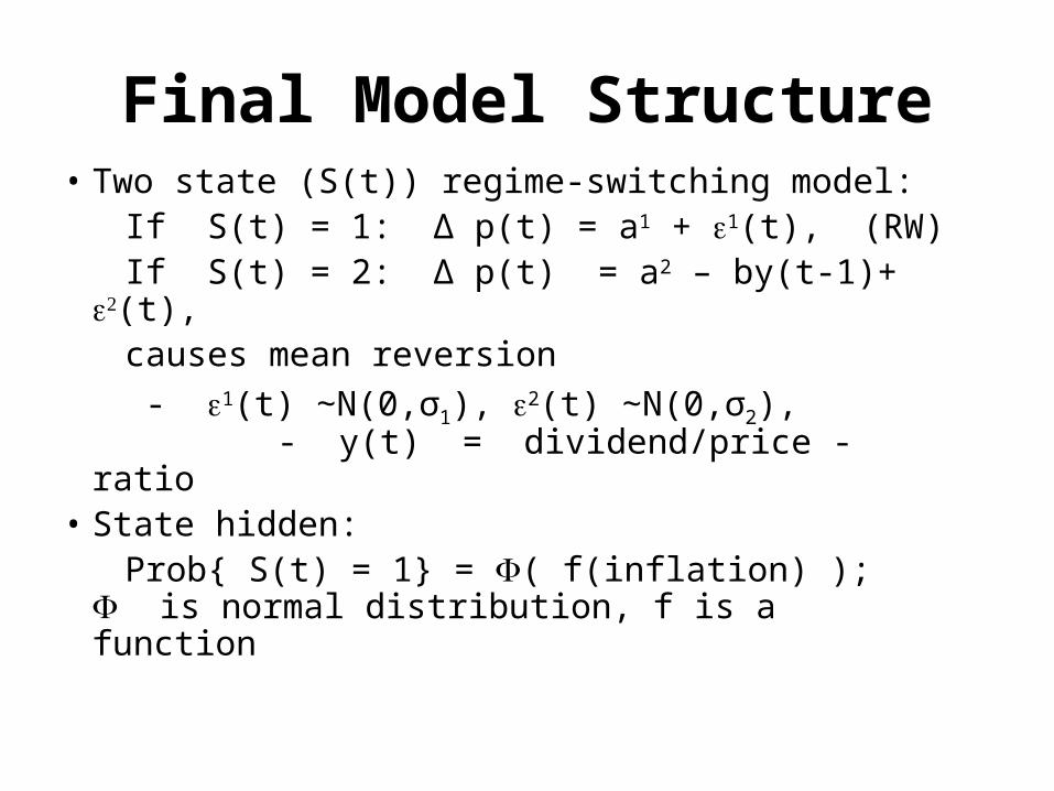
Final Model Structure• Two state (S(t)) regime-switching model: If S(t) = 1: Δ p(t) = a1 + 1(t), (RW) If S(t) = 2: Δ p(t) = a2 – by(t-1)+ (t), causes mean reversion
- 1(t) N(0,σ∼ 1), 2(t) N(0,σ∼ 2), - y(t) = dividend/price -ratio
• State hidden: Prob{ S(t) = 1} = ( f(inflation) ); is
normal distribution, f is a function

Statistical Model for Dividend and Inflation
• Dividend: AR(2)-ARCH(4) –model
- Dividend is the driving factor.
• Inflation: AR(4) –model where dividend is explanatory variable
- Note! This is just statistical relation, not causal. See fig on cross-correlation!
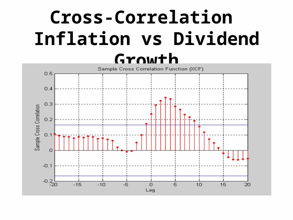
Cross-Correlation Inflation vs Dividend Growth

Price Dynamics
Log-Likelihood method results in the
following significant relation:
S(t) = 1: Δ p(t) = 0.027 + 1(t)
S(t) = 2: Δ p(t) = 1.078 – 0.357y(t-1)+ (t),
- 1(t) N(0,0.052), ∼ 2(t) N(0,0.077)∼• Return distribution conditional:
State S(t) and y(t) = log(P(t) /D(t))
Model Testing
• The model is compared to 1) more general and 2) linear alternatives:
- More general LMARX (that include standard RW and more complicated models) is rejected at 5 % level
- Information criterion AIC and BIC select the nonlinear model instead of linear one

Model Diagnostic
• Quantile (QQ) –plot shows:
- Normal distribution assumption for the residuals of the linear model is wrong (fig)
• Quantile residual plot shows:
- Excellent fit for LMARX
See fig. (Can see that it is not from normal distribution?)
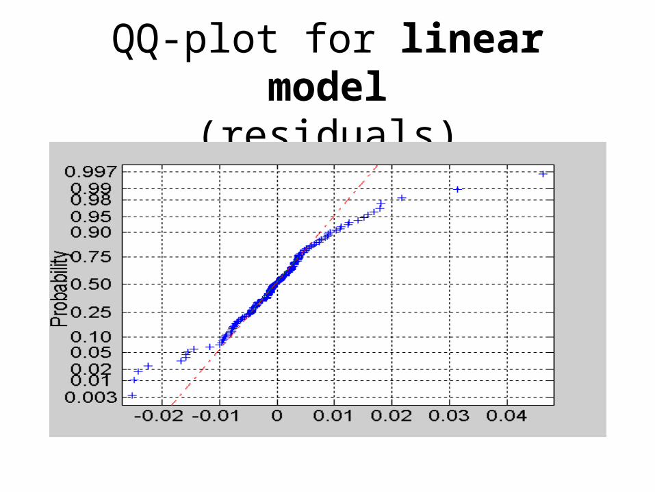
QQ-plot for linear model(residuals)
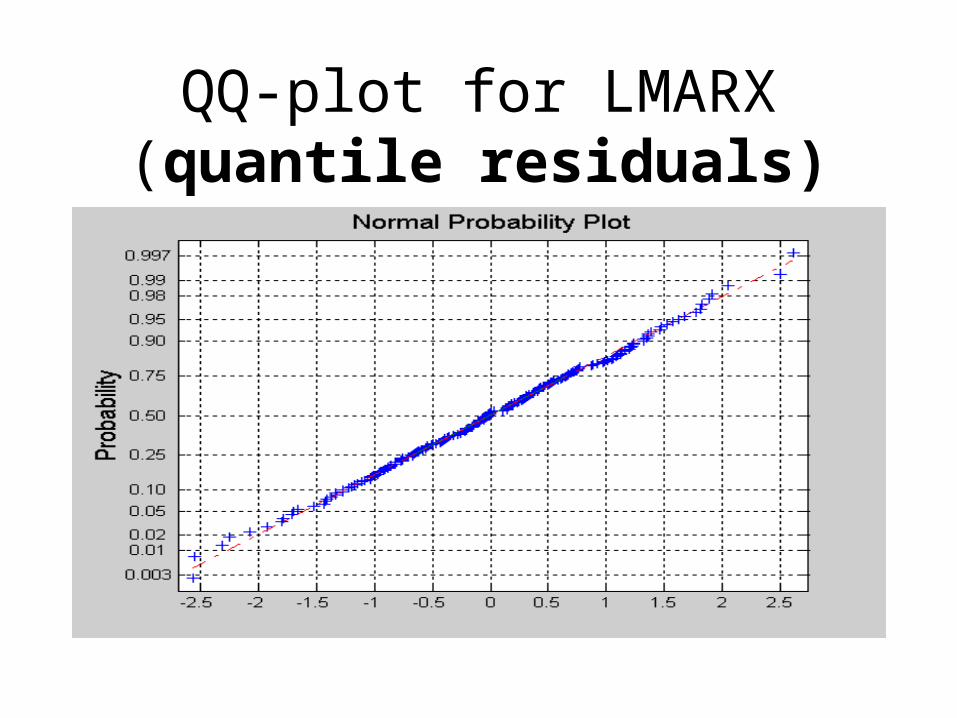
QQ-plot for LMARX(quantile residuals)

Prob{S=2 } as a function of inflation - High inflation is tricker for state-switch
Intrerpretation• Model operates much more often in state 1
than in state 2; that is RW is a good description most of the time
• E(Δ d) = 0.014 < 0.027 = E(RW | S =1).
=> process generates bubbles
=> switch from S=1 to S=2 causes a market crash, since b < 0 (b is the coefficient of log(P(t) /D(t)) in state 2)
=> process is mean reverting

UK – data (not in the paper)
• Overfitting is a danger especially when nonlinear model is used
=> We tested also the UK -data
=>The model structure remains invariant (heteroscedastic residuals)
Risk Assessment
• The proposed model has shape-changing predictive distribution
• Shape depends on
- prediction horizon
- inflation
- P/D –ratio
=> Risk is time-varying
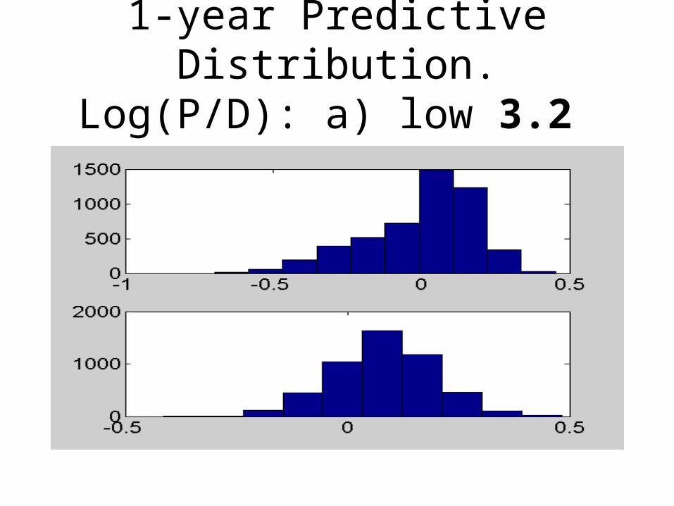
1-year Predictive Distribution.Log(P/D): a) low 3.2 b) high 3.8

1-year Predictive Distribution.Log(P/D) is 3.8, Inflation 4 %
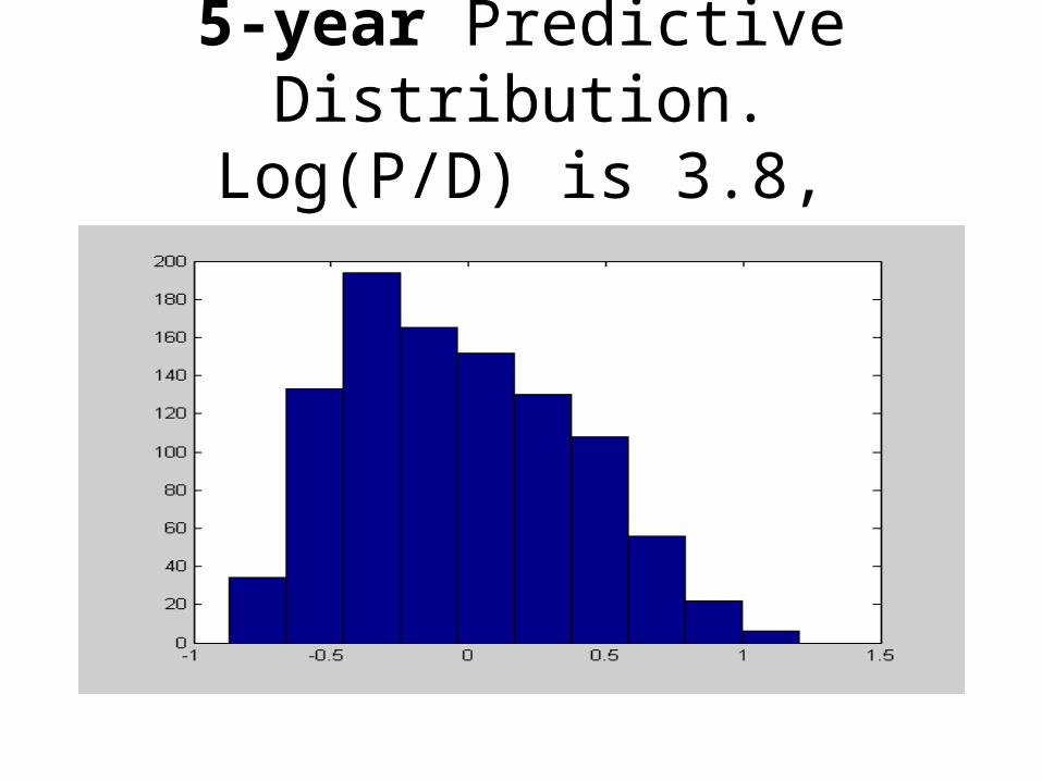
5-year Predictive Distribution.Log(P/D) is 3.8, Inflation 4 %

10-year Predictive Distribution.Log(P/D) is 3.8, Inflation 4 %

Present Situation
• Good: Stock market risk is much lower than in 2000
• Bad: P/D –ratio still high in the U.S.