May 17, 2001

Dynamic Imagery:A Computational Model of Motion and Visual Analogy

David Croft and Paul ThagardUniversity of Waterloo

Abstract:

This paper describes DIVA (Dynamic Imagery for Visual Analogy), a

computational model of visual imagery based on the scene graph, a powerful

representational structure widely used in computer graphics. Scene graphs make possible

the visual display of complex objects, including the motions of individual objects. Our

model combines a semantic-network memory system with computational procedures

based on scene graphs. The model can account for people’s ability to produce visual

images of moving objects, in particular the ability to use dynamic visual analogies that

compare two systems of objects in motion.

Address for correspondence:

Paul Thagard, Philosophy Department, University of Waterloo, Waterloo,

Ontario, Canada, N2L 3G1. E-mail: pthagard@uwaterloo.ca.

2

Dynamic Imagery:A Computational Model of Motion and Visual Analogy

David Croft and Paul ThagardUniversity of Waterloopthagard@uwaterloo.ca

INTRODUCTION

How is a gymnast’s cartwheel like a windmill? Answering this question cannot

rely just on the verbal information that we have about gymnasts and windmills, or just on

the static visual images we have of them. Rather, the comparison becomes interesting

when we mentally construct dynamic images of a person whose limbs are in motion and a

windmill whose blades are turning.

Mental imagery is often used to visualize a static scene, but it can also be

dynamic, when people imagine objects in motion. For example, Pedone, Hummel, and

Holyoak (in press) found that the use of animated diagrams significantly improved

analogical problem solving. How do people construct and use dynamic mental images?

It has become increasingly accepted that problem solving sometimes uses mental imagery

that employs pictorial representations in addition to the verbal representations that

commonly support problem solving (Larkin and Simon, 1987). But little research has

been done on how people represent motion and use it in analogical problem solving and

other kinds of thinking.

This paper describes a computational model of dynamic imagery based on a

powerful representational structure widely used in computer graphics, the scene graph.

We hypothesize that human thinking uses dynamic representations that have some of the

same computational powers. Scene graphs employ a hierarchical organization that makes

possible the visual display of complex objects, including the motions of individual

3

objects. Organizing visual information in a hierarchy allows motions to be represented

as discrete behaviors that can be applied to specific objects in a scene. We adapt this

technology to explain how the mind can apply motions to objects that it has not

previously seen in action. For example, people can imagine a computer monitor falling

off a desk even if they have never previously perceived such an event.

This paper describes a computational model of human dynamic imagery that

combines a semantic-network memory system with computational procedures based on

scene graphs. We have exploited the computational power of a recently developed

programming library, Java 3D, to model how people are able to construct and transform

complex visual scenes. Our model simulates visual operations such as object

combination, rotation, and imagined motion, as well as mapping of scenes in dynamic

visual analogies. We will argue that the scene graph representation makes possible a

computationally and psychologically richer account of mental imagery than has

previously been achieved in cognitive science and artificial intelligence (see the

comprehensive collection of papers in Chandrasekaran, Glasgow, and Narayanan, 1995).

ARCHITECTURE AND REPRESENTATION

Dynamic imagery requires a cognitive architecture that uses working memory to

integrate and operate on representations derived from perception and long term memory.

After describing our theoretical assumptions about the interactions of perception and

memory, we will describe how scene graphs can be used for the representation of visual

information including motion.

4

Perception and Memory

Our model of dynamic imagery assumes that mental imagery is tied in with three

major processing systems: perception, working memory, and long-term memory.

Perception provides the input, and long-term memory serves as a high-level store that

integrates visual memories with semantic information. Working memory serves as the

arena for combining and processing visual information, as illustrated in Figure 1. The

large arrows in Figure 1 emphasize the two-way interaction and ongoing exchange of

information between the two memory systems. Later, when we present our computational

model of dynamic imagery, we will say much more about the processes involved in

perception and memory.

The world Working memory Long-term memory

Perception

Visual Buffer

Figure 1. Processing systems contributing to mental imagery.

Our model emphasizes the organizational role of long-term memory in mental

imagery. For example, given a visual concept such as dog, long-term memory stores

images of particular dogs derived from perception, and it also provides non-visual

information about how dog relates to other concepts (eg. dog isa animal, Spot isa dog).

Working memory serves to extract and compare visual concepts, as well as to update our

visual database when a novel concept is imagined. For example, you can imagine a

futuristic all-terrain vehicle with no wheels but rather large spider-like legs for moving it

5

about. Imagining involves retrieving from long-term memory visual representations of

concepts such as vehicle and spider, combining the two together in working memory, and

finally storing the assembled spider-vehicle back into long-term memory. Similarly,

processing the cartwheel-windmill analogy requires retrieving from long-term memory

representations of gymnasts and windmills derived from previous perceptions, then using

working memory to analyze motion similarities between the two concepts. Working

memory is able to infer information that was not previously stored in long-term memory,

as when we answer the question: How many dialing keys are there on a standard phone?

To answer this question, our working memory constructs a mental image of the telephone

and we can count the 12 keys.

Scene Graphs as Mental Representations

What is the representational format in which visual information is stored in long-

term memory and manipulated in working memory? Skeptics about mental imagery

such as Pylyshyn (1984) maintain that no special pictorial representations need to be

postulated, but there is much evidence that human thinking employs visual as well as

verbal representations (e.g. Larkin and Simon, 1989; Kosslyn, 1994). But the exact

nature of these visual representations remains a major problem in cognitive science. It is

not helpful to think of them as collections of pixels like the display on a computer screen,

because a pixel representation does not support operations such as object combination

and motion analysis.

The image in Figure 2 could in principle be decomposed into a verbal

representation such as “There is a rectangle with a circle on the left half, and a star on the

right half. A pyramid of three triangles is centered inside the circle.” The verbal

6

representation, however, awkwardly makes inferences that are automatic from a visual

representation, such as that the top triangle is to the left of the star. A pixel

representation would not support interesting visual operations such as imagining that the

star moving into the circle and that the triangles moving to the original location of the

star.

Figure 2. Image containing a discrete set of objects

The human mind has to organize visual information in a way that enables

complex visual inputs to be broken apart, stored and recombined to form new wholes.

Computer graphics researchers have converged upon the idea of a 'scene graph' to

represent visual information. A scene graph is a hierarchical representation that provides

a powerful means of representing the world. It consists of an inverted tree in which each

branching point or leaf of the tree is used to store a piece of information about a visual

scene. This piece of information could be about the size of an object, the position of a

group of objects, or the color of an object. Any branching point or leaf of the tree is

referred to as a node. Figure 3 shows how the picture in Figure 2 can be translated into a

hierarchical scene graph.

7

rectangle

circle

triangle 1

triangle 2

triangle 3

star

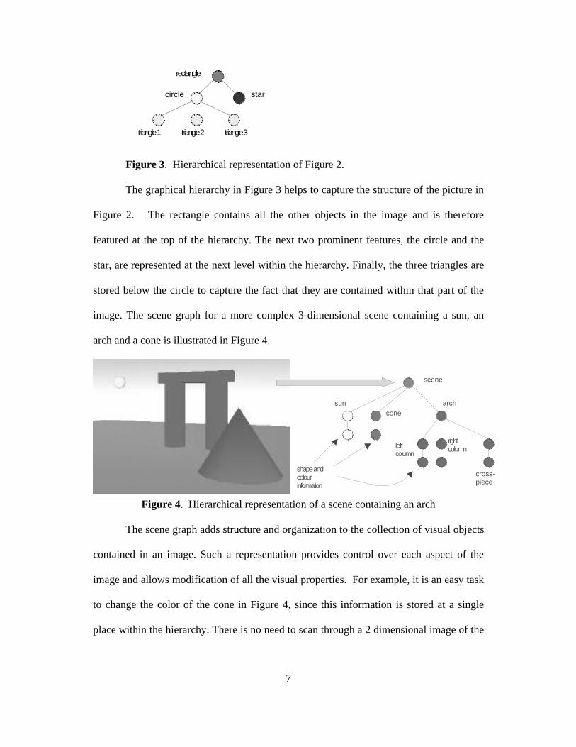
Figure 3. Hierarchical representation of Figure 2.

The graphical hierarchy in Figure 3 helps to capture the structure of the picture in

Figure 2. The rectangle contains all the other objects in the image and is therefore

featured at the top of the hierarchy. The next two prominent features, the circle and the

star, are represented at the next level within the hierarchy. Finally, the three triangles are

stored below the circle to capture the fact that they are contained within that part of the

image. The scene graph for a more complex 3-dimensional scene containing a sun, an

arch and a cone is illustrated in Figure 4.

sun

scene

cone

arch

shape and colour information

left column

right column

cross- piece

Figure 4. Hierarchical representation of a scene containing an arch

The scene graph adds structure and organization to the collection of visual objects

contained in an image. Such a representation provides control over each aspect of the

image and allows modification of all the visual properties. For example, it is an easy task

to change the color of the cone in Figure 4, since this information is stored at a single

place within the hierarchy. There is no need to scan through a 2 dimensional image of the

8

arch-scene and modify the color of each cone-pixel. It is important to note that the scene

graph representation is also viewpoint independent.

Procedures such as translation or rotation are controlled by adding nodes to the

graph structure. For example, a node could be added to rotate an object contained in the

graph. If a rotation node was placed above the section of the graph containing the

information for the arch, the entire arch would be rotated while maintaining the spatial

relationship between the pieces of the arch.

Representing Motion

Unlike verbal and pixel representations, scene graphs provide a powerful means

to store and process motion. Consider the example illustrated in Figure 5, and imagine

the car driving down the road, losing control, and swerving off the road. Scene graphs

provide a way of representing the motion of the car by inserting nodes into the graph that

describe the motion of an object. These motion nodes, called behaviors, contain

information about how a property of an object changes over a given period of time. Any

property of an object can change over time, whether it be position, shape or color.

Multiple behavior nodes can be added into a visual hierarchy to represent complex

changing scenes. For example, one behavior node might specify the pathway of the car

swerving off the road and hitting the tree. Another behavior node could specify that after

the collision, the tree falls down across the hood of the car.

9

Figure 5. Car crash – an example of motion in visual images.

Note the advantage of associating motion with particular objects in the form of

behaviors rather than with the entire scene. Dynamic images are not like movies

retrieved from memory and run as a whole. Rather, individual visual concepts can be

combined with behaviors to create any number of novel scenarios. We can imagine the

car in Figure 5 starting up and driving around all the trees, or even the trees starting to

dance away from the car. In scene graphs, complex motions can be decomposed into a

set of interpolations that model the behavior of an object. For example, a simple

interpolator behavior could specify the path followed by the car moving from one tree to

another.

To model the revolution of one object around another, a behavior node can be

added to the graph that specifies the rotation of an object about a central point over a

given period of time. The scene graph for a simple model of an atom in which the

electrons orbit the nucleus is shown in Figure 6, which shows how information about

dynamics can be stored within the graph representing a visual scene.

10

atom

nucleus

electron orbits

dynamics info

shape and size info for electrons shape and size info for proton and neutron

Figure 6. Scene graph for an atom with rotational behavior nodes added for each

electron.

Behavior nodes can be combined together to create very complex motions. For

example, starting with a 3-dimensional representation of a stick-man, an interpolator

behavior can be added to each arm that changes its position over time. Done properly,

these interpolators can simulate the swinging motion we observe watching the arms of

someone walking down the street. Similarly, an interpolator can be added to each leg that

simulates the stepping motion. The scene graph for this construct would look something

like that illustrated in Figure 7. Some interpolator behaviors require many co-ordinates in

their path to accurately simulate a motion. For example, a simple orbital motion only

requires a radius for the pathway and a point of rotation, whereas the pathway followed

by a human leg in an average step would require an accurate representation of the

rotation and acceleration at the hip, the knee, and the ankle.

11

stick-man

body

head

legs

arms

Figure 7. Scene graph for a stick man with behaviors that represent walking.

The use of behaviors within a visual hierarchy permits a dynamic scene to be

represented in a very compact fashion, not as a complete movie composed of 2-

dimensional images where each image is slightly different from the others. If people

stored dynamic scenes in movie-like format, we would not be able to create new movies,

let alone solve problems that involve reasoning about the motions involved. Our ability to

compose mental movies relies upon the creative ability to combine behaviors with static

visual concepts stored in our long-term memory. For example, our minds are able to

visualize a cat typing at the computer even though we have probably never perceived this

situation. To visualize the typing cat, we transfer the behaviors responsible for the human

typing motion to our representation of the cat.

Evidence for a recombinant set of motions in human thinking is provided by the

dream research of Hobson (1988). He carefully analyzed the dream journal of “Engine

Man” who copiously recorded his dreams over a 3-month period in 1939. Of the 110

diagrams contained in Engine Man’s dream entries, 25 contain explicit representation of

12

“dream trajectories” that use a dashed line to represent the path and an arrowhead to label

the direction. These trajectories describe a set of motions that could be represented as

behaviors in scene graphs.

In sum, scene graphs have many advantages as a form of representation for visual

information and imagery. First, their hierarchical form enables them to capture a broad

range of information about the properties of objects and the relations between them.

Second, the inclusion of behaviors in scene graphs makes possible the representation and

simulation of complex motions and allows novel scenes to be created from a finite set of

objects and motions. Third, scene graphs are computationally feasible - in fact, this

representation was developed by the computer graphics community for applications such

as virtual reality and digital animation. Before going into the details of how we have

implemented scene graphs in our own computational model, we will contrast them with

alternative computational means of representing visual information.

Comparison with Other Methods of Visual Representation

The first computational model of visual problem solving was developed by Funt

(1980), who represented diagrams using square arrays inspired by the retina as a special

purpose parallel processor. He did not, however, attempt to represent the organization of

scenes or the motions of objects. Forbus (1995) and his colleagues developed the PV /

MD model of qualitative spatial reasoning, in which spatial representations consist of two

parts: a metric diagram, which includes quantitative information and thus provides a

substrate which can support perceptual-like processing, and a place vocabulary, which

makes explicit qualitative distinctions in shape and space relevant to the current task.

This model is useful for reasoning about the behavior of mechanisms such as clocks, but

13

is not proposed as a general theory of human visualization. Chella, Frixione, and Gaglio

(2000) propose a framework for the representation of visual knowledge in a robotic agent

to understand dynamic scenes, using a combination of high level verbal descriptions and

low level conceptual spaces realized by time-delay neural networks. Their architecture

is plausible for recognizing dynamic scenes, but does not use visual representations to

manipulate and make inferences about them.

Glasgow and Papadias (1992) presented a broad and insightful theory of

computational imagery based on a formal theory of arrays and implemented in the array-

based programming language Nial. An array is a collection of items held at positions in a

rectangular arrangement along multiple axes. Arrays serve well to capture spatial

relations such as left-of and north-of, and can be nested to capture hierarchical

information. For example, the picture in Figure 2 could be represented by an array of two

items, a circle and a star, with another array nested inside the circle containing 3

triangles. Unfortunately, because of their rectangular organization, arrays are somewhat

limited in their ability to represent spatial relations. It is not clear, for example, how an

array can capture the information that a single top triangle is over both of the lower

triangles. Moreover, the array formalism does not, to our knowledge, support any means

of putting arrayed objects in motion. Hence for developing a computational model of

dynamic imagery, scene graphs appear superior to arrays as a representational

mechanism.

Tabachnik-Schijf, Leonardo, and Simon (1997) proposed the CaMeRa model of

multiple representations to explain how experts use diagrammatic and verbal

representations to complement each other. In this model, pictorial information consists of

14

a bitmap and associated node-link structures. The latter enable CaMeRa to represent

hierarchical information in ways similar to scene graphs, but this model has no means to

represent and make inferences about objects in motion. We will now provide

computational details about how scene graphs can be used to model dynamic imagery.

COMPUTATIONAL IMPLEMENTATION

We have developed a computer program which produces animated visual displays

and which can be used for simulating visual analogies involving motion. The program is

called DIVA: Dynamic Imagery for Visual Analogy. DIVA is written in the language

Java, which includes a library named Java 3D for representing and animating 3-

dimensional information. Java 3D uses scene graphs in which different types of nodes

store different pieces of information. Some nodes are used to group objects together,

whereas another type of node might specify a translation or rotation. Behaviors are

represented as another type of node that includes information about changing properties

of an object, whether it be position, shape or colour. Technical details about Java 3D can

be found at the Web site: http://java.sun.com/products/java-media/3D/. DIVA combines

visual representations based on scene graphs with a network that represents semantic

components of long-term memory. Simulated perceptual input to the program is

provided by VRML, a tool developed to exchange and display 3-dimensional models on

the Web.

Perception via VRML

The Virtual Reality Modeling Language (VRML) was developed to serve as a

standard means of representing 3-dimensional information on the Internet (see

http://www.vrml.org). The second proposed standard for VRML was called Moving

15

Worlds, reflecting the fact that it permits motion information to be included within a

model. VRML is a text-based descriptive file format, not a full-fledged programming

library, and consequently does not provide any tools for manipulating 3-dimensional

scenes.

We use VRML for input into DIVA because there is an abundance of VRML

models available on the Internet. VRML models of common objects, from chairs to

castles to avatars (human shapes), are easily located on the Internet and parsed into the

program. This allows us to simulate perception without having to create our own visual

representations.

Working Memory via Java 3D

Java 3D provides the representation and some of the processing for DIVA’s

working memory component. Java 3D provides functionality to parse the text-based

VRML files and load them into memory as a scene graph. This 3-dimensional structure

can then be rendered to the screen of the computer from any viewing perspective.

Information is extracted from the scene graph by traversing up, down or across the graph

and querying information stored at each node. Some examples of the types of node used

within the Java 3D scene graph are:

• Transform: specifies a translation, rotation or scale for all children below this node.

• Group: groups one or more children nodes together.

• Shape: specifies a shape using geometric primitives such as squares and spheres or

using complex groupings of triangles to represent curved or irregular surfaces.

• Material: specifies a color or texture that should be applied to the 3 dimensional

surface of a shape node.

16

• Behavior: specifies a changing condition such as movement for some section of the

scene graph.

Java 3D assembles the information from all the nodes in the scene graph into a 3-

dimensional model that can be viewed on the computer screen.

Java 3D provides a rich set of behaviors that can be added to a scene graph. These

include rotation interpolators (such as the motion of planets about the sun), complex path

interpolators (such as walking through a winding wilderness trail) and scaling

interpolators (something that grows or shrinks over a period of time). All of the

interpolators operate using x, y and z co-ordinates to describe positions, and matrices to

describe rotations about one or more of the x, y or z axes.

Java 3D includes functionality for specifying the location where the viewer is

looking at the current visual scene. For example, if we load in a VRML model of a car,

we can view the car from an external perspective watching it drive by the street, or from

the perspective of the driver sitting behind the steering wheel. Given a certain perspective

or ‘viewpoint’, the Java 3D library is able to convert the 3-dimensional model into a 2-

dimensional image that can be observed on the computer monitor.

The operation of working memory in DIVA employs built-in Java 3D functions

for simulating basic operations such as translation, rotation and scaling. These operations

involve finding and modifying a node within the scene graph.

Long-term Memory via a Semantic Network and Scene Graphs

Long-term memory can be thought of as a database containing memories of

sensory input and relationships between these memories. It requires storage of visual

scenes, but also includes semantic information about objects or abstract concepts that we

17

have learned. Our program models long-term memory using a structure like the semantic

networks in the ACT model of Anderson (1983). It can store simple propositions such as

“stick-man is drawing.” or “stick-man represents human.” A concept such as stick-man

is represented by a node within the network, and is defined by its associations with other

nodes.

It is important to distinguish between a node within the semantic network, which

represents a complete concept, and a node within a scene graph, which is simply part of a

hierarchy representing a single visual object. A node within a semantic network can have

a chunk of encoded data attached to it that stores a visual representation. For example, a

stick-man node in a semantic network might have a scene graph structure attached to it

that could be decoded in working memory and viewed. Figure 8 illustrates the

relationship between a scene graph and the overall semantic network.

legs

body

head

arms

stick-man

drawing

human

land 3D input Semantic network

walks-on

is is

Scene graph attached to the stick-man concept

represents

Figure 8. A concept in the semantic network can have a scene graph

attached to it that stores the visual representation.

18

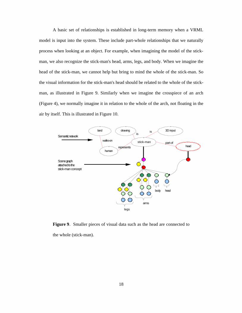
A basic set of relationships is established in long-term memory when a VRML

model is input into the system. These include part-whole relationships that we naturally

process when looking at an object. For example, when imagining the model of the stick-

man, we also recognize the stick-man's head, arms, legs, and body. When we imagine the

head of the stick-man, we cannot help but bring to mind the whole of the stick-man. So

the visual information for the stick-man's head should be related to the whole of the stick-

man, as illustrated in Figure 9. Similarly when we imagine the crosspiece of an arch

(Figure 4), we normally imagine it in relation to the whole of the arch, not floating in the

air by itself. This is illustrated in Figure 10.

legs

body

head

arms

stick-man

drawing

human

land 3D input

Semantic network walks-on

is is

Scene graph attached to the stick-man concept

represents head part-of

Figure 9. Smaller pieces of visual data such as the head are connected to

the whole (stick-man).

19

semantic network

columns

arch part-of crosspiece

scene graph

crosspiece

Figure 10. Relation of the concept of a ‘crosspiece’ in the scene graph of an arch

DIVA uses a simple mechanism for exchanging information between long-term

memory and working memory. Concepts can be retrieved from memory using their

names or by association with concepts that might already be active in working memory.

For example, a working memory process could retrieve all the concepts that are

associated with arch. These might include column, crosspiece, support, or Romans,

depending on the semantic associations that have been input into the model. The long-

term memory system is able to extract associated concepts using spreading-activation

algorithms similar to those in ACT.

Scene Manipulation via a Graphical Interface

In addition to the VRML perceptual input and the working and long-term memory

processes, DIVA has a graphical interface that allows a user to view three-dimensional

scenes, browse the long-term memory structure, and input commands to the program. A

command-line enables the user to control the actions of the program. For example, a

command such as “rotate gearbox y 30”, would load the visual information for a gearbox

into working memory, rotate the model 30 degrees about the y axis, and display the

resulting scene to the lower-left window of the user interface. Providing the program

20

with such input commands enables it to simulate how people intentionally manipulate

their mental images.

MODELING VISUAL ANALOGIES

Dynamic imagery can contribute to many important kinds of thinking, including:

• Problem solving, when we imagine objects (possibly ourselves) moving physically

from a starting position to a goal;

• Diagnosis, when we visualize the operation of a physical device or biological system

to determine why it is faulty;

• Thought experiments, when scientists imagine unusual motions to draw insights

about the principles governing the motions of objects.

Our modeling efforts to date have largely concentrated on simulating visual analogies

which involve comparisons of visual representations, including ones in which the source

and target analogs both involve objects in motion.

Algorithm for Analogical Mapping of Scene Graphs

If visual images are represented by scene graphs, then the problem of finding

analogies between images is at least as hard as the computational problem of subgraph

isomorphism, which requires deciding if there is a subgraph of one graph which is

isomorphic to another graph. This problem is known to be NP-complete, that is, it

belongs to a large class of problems that are believed to be computationally intractable.

However, visual analogical mapping can be performed by an algorithm adapted from the

constraint-satisfaction algorithm used for mapping verbal representations in the program

ACME (Holyoak and Thagard, 1989). DIVA performs analogical mapping by creating a

constraint network representing possible mappings between a source and target scene

21

graph and then uses a connectionist algorithm to settle the network and select the best

mappings between the two graphs.

Creating the constraint network requires generating mapping hypotheses

concerning the possible correspondences between the nodes in the two scene graphs,

establishing positive constraints between mapping hypotheses that fit together, and

establishing negative constraints between incompatible mapping hypotheses. Here is an

outline of the algorithm that generates mapping hypotheses and positive constraints, and

then selects the best mappings. The visual similarity comparison made in the first step of

the algorithm is discussed in the next section.

1. For each node Si in the source scene graph, search through the nodes in the target

graph, identifying each Tj that is visually similar to Si.

2. Create a mapping unit Si=Tj that hypothesizes that Tj corresponds to Si.

3. Create a positive constraint (symmetric excitatory link) between a SPECIAL unit that

is always active and each mapping unit concerning two nodes that are visually similar.

The weight on these links is proportional to the degree of visual similarity between the

two nodes.

4. For the parent node SiP of Si and the parent node TjP of Tj, create a mapping unit

SiP=TjP, unless (as is often the case) it has been already been created. Establish a

positive constraint between Si=Tj and SiP=TjP, i.e. make a symmetric excitatory link

between the two units.

5. For each pair of incompatible mapping units, e.g. Si=Tj and Si=Tk, create a negative

constraint using inhibitory links between the units, so that the two hypotheses militate

against each other.

22

6. Spread activation through the network until it settles. For each node Si in the source

scene graph, determine which mapping unit Si=Tj has the highest activation, which

indicates that Tj is the best mapping for Si.

This algorithm is similar to the one used in ACME in that it employs the

constraints of similarity and structure that are part of the multiconstraint theory of

analogy (Holyoak and Thagard, 1995), but it implements the constraints based upon the

scene graph representation. In ACME, similarity is semantic similarity, whereas DIVA

uses visual similarity as defined below. Unlike ACME, DIVA uses similarity to help

limit the number of mapping hypotheses; in this respect it is like the DRAMA model of

analogical mapping between distributed representations (Eliasmith and Thagard,

forthcoming). As in ACME, one-one mappings are encouraged by the inhibitory links

established by step 5 of the algorithm, but they are not strictly required as they are in the

SME model (Gentner, 1983; Falkenhainer, Forbus, and Gentner, 1989).

Step 4 of the algorithm that establishes constraints between parent-child mappings

(Si=Tj and SiP=TjP) is an essential aspect of the algorithm since it conserves the

structural organization of the source and target scene graphs. The parent-child constraints

help to conserve relational consistency or parallel connectivity: R(a,b) tends to map to

S(c,d) only if R tends to map to S, a tends to map to c, and b tends to map to d. In the

scene graphs there is no verbal representation of relations and objects, so relational

consistency is established by connecting mappings between nodes with mappings

between their parents as specified in step 4.

Visual Similarity in Scene Graphs

23

Step 1 of the algorithm for mapping between scene graphs requires a way of

computing the visual similarity of two nodes. This is accomplished by considering the

type of each node, and then querying the properties corresponding to that node type. Only

nodes of the same type are compared, as a node that represents a transform will never

map with a node representing a shape. A very important aspect of the visual similarity

comparisons is that wherever possible, a ratio is established that represents the degree of

visual similarity. For example, if we are comparing two group nodes, Si and Tj, if Si has

2 children and Tj has 3 children, then a similarity ratio of 2/3 = 0.667 is used as the initial

activation for the mapping unit between these nodes. This reduces the number of hard-

coded variables in the model, and makes flexible comparisons between nodes of the same

type. Unlike ACME, which implements similarity constraints by means of differential

weights from a special, always active units to units representing mapping hypotheses,

DIVA implements similarity constraints by means of differential initial activations of

units representing mapping hypotheses.

Another important aspect of the similarity comparisons is that wherever possible,

comparisons are made relative to the overall dimensions of the scenes. For example, if a

50m-wide field contains a pyramid with a 10m a base, this would be considered visually

similar to a pyramid-shaped object with a base of 10cm sitting on a 50cm-wide tabletop.

The two pyramid objects are the same size relative to the scenes that contain them. The

specific similarity comparisons that establish the initial activation for a mapping unit

between a source node Si and a target node Tj are as follows:

24

1. If the nodes are both group types, which group subordinate nodes together, then the

initial activation for this mapping unit will be a ratio of the number of children for

each group node. Group nodes with only one child are ignored.

2. If the nodes are both transform nodes, which specify three-dimensional translation,

rotation, or a scaling factors, then establish a similarity ratio based upon the 4x4

matrices containing the x, y, z translation, rotation and scaling information. This is a

detailed comparison involving considerable matrix algebra. Note that the ratio is

made relative to the size of the scenes containing the transforms.

3. Some nodes include group and transform information (items 1 and 2 above), and if

this is the case, the similarity ratio is composed of the group similarity in addition to

the transform similarity. The consequence of this is that some nodes can have

similarity ratios greater than 1.0 (but still always less than 2.0).

4. If the nodes represent a primitive shape (eg. box, cylinder, sphere, cone), then

establish a similarity ratio only if the nodes represent the same type of shape (eg. both

nodes represent a sphere), and make the initial ratio based upon the dimensions of the

objects. Again, the ratio is made relative to the size of the scene containing each

object.

5. If the nodes represent an irregular geometric shape, then compare the arrays

containing the vertices for this shape. After comparing the co-ordinates for each

vertex, establish a ratio that is the average for all the vertices. Note that vertices are

compared relative to the size of each shape.

6. If the nodes represent a shape (items 4 and 5 above), it is possible they also contain

appearance information. If the appearance for both nodes is a color value specified

25

using three decimals representing red-green-blue colour components, then establish a

ratio based upon these decimals. For example, the color value red (1, 0, 0) would

compare with another color (1, 0.5, 0) with a ratio of (1.0 + 0.5 + 1.0)/3 = 0.833. The

ratio that is established for the similarity of the appearance is then added to the ratio

generated in steps 3 and 4. Note that this will potentially generate a similarity ratio

greater than 1.0 (but still less than 2.0). By enabling nodes to have an activation

greater than 1.0, nodes that contain two types of properties (group and transform

information, or shape and color information) are able to stand out amongst other

nodes that specify only a single piece of information.

7. If the nodes are both behavior nodes that contribute to a specific motion pattern (eg.

convergence), then a comparison is made based upon the type of motion pattern. For

example, if both the scenes contain a convergence pattern, then behavior nodes are

compared based upon the angle and pathway they follow when converging towards

the center of the scene.

An example that illustrates the application of the visual similarity algorithm is a

scenario between two scenes that both contain arch-like shapes. In the first scene, shown

on the left side of Figure 11, the arch is composed of rectangular columns with a block

resting on top. In the scene on the right side of Figure 11, the arch is red in colour,

slightly to the right and built with larger cylindrical columns (this is the same scene

illustrated in Figure 4). Note than both scenes contain a sun-like shape in the sky, and

ground upon which the arches rest.

26

Figure 11. Comparison between two scenes containing arch-like shapes.

The output of DIVA’s visual similarity algorithm that analyzes the scenes illustrated

in Figure 11 is shown in Figure 12. There are a few things to notice in Figure 12. First,

the output appears quite busy since the complete graph for both scenes has been drawn.

The second thing to notice is that the 3 arcs drawn between the two graphs represent the 3

most prominent mappings after the constraint network has settled. In total there were 43

mappings and 103 constraints within the constraint network. The top three mappings

established by the algorithm are as follows.

First, the most prominent mapping illustrated in Figure 12 is between the two group

nodes that collect together the four major objects in each scene (the sun, ground,

box/cone, and the arches). This corresponds to the top-most arc illustrated in Figure 12

and has a settled activation of 1.83. Initially this mapping has a value of 1.0, since both

group nodes have four children. However, since there is also a mapping for each child

node (there is a mapping between the two suns, the two ground surfaces, the two different

box/cone shape, and the mapping between the arches) the activation from these mappings

spreads to the parent mapping. This result indicates that when all the objects are

considered, the two scenes are highly analogous.

27

The second most prominent mapping after the constraint network has settled is

between the two nodes representing the arches (this is the bottom-most arc in Figure 12

and has a settled activation of 1.75). This result is very important since it recognizes the

‘whole’ that establishes the arch-like shapes. Initially, the mapping between the two

group nodes that represent the arches only has a value of 1.2, since both nodes have the

same number of children (ratio of 1.0), and since they are roughly in the same position

(ratio of 0.2). The value of this mapping is considerably less than many of the other

mappings that are initially established. For example, the initial mapping between the two

ground surfaces has the maximum value of 2.0 (1.0 since they are exactly the same

geometric shape, and another 1.0 since they are exactly the same color). However,

because the constraint network conserves the structural relationship of the scene graph,

the mappings between the columns of each arch and between the crosspiece feed

activation to the parent mapping representing the arch. This is a major strength of the

constraint network approach as it identifies the ‘wholes’ that are composed of a number

of pieces (two columns and a crosspiece).

Finally, tied for second is the mapping between the Shape3D nodes that

represents the ground in both scenes. This is represented by the middle arc in Figure 12

and also has a settled activation of 1.75. These two nodes have an identical shape (1.0

similarity) and are also the same color (1.0 similarity), giving the mapping an initial

activation of 2.0. It is interesting to note that although the mapping between the ground

shapes has twice the initial activation compared to the most prominent mapping between

the group nodes described in (1), it ends up with less activation due to the structural

properties of the graph. This illustrates the effectiveness of the constraint network at

28

capturing structural relationships. After the constraint network has settled, the mapping

between the ground surfaces only has a value of 1.75, whereas the mapping between the

group nodes in (1) has a value of 1.83.

Another interesting result illustrated by Figure 12 is that the mapping between the

two ground surfaces has a higher settled activation than the mapping between the sun-like

objects represented by the left-most branch of the two graphs. Both these mappings start

with an initial activation of 2.0, since their respective objects are the same shape and

color. After the constraint network has settled, the mapping between the sun-like shapes

only has a value of 1.63 (this is the ninth-most prominent mapping). This is likely

because the mapping between the ground surfaces is directly connected with the most

prominent mapping in the constraint network (between the two group nodes illustrated by

the top-most arc in Figure 12). The mapping between the sun-like shapes is one-level

removed from most prominent mapping, and therefore does not receive as much

activation as the network settles.

Figure 12. Top 3 mappings output by DIVA's visual similarity algorithm for the

arch example.

29

Another example that demonstrates the ability of DIVA’s visual analogy algorithm to

recognize whole shapes are the two scenes illustrated below in Figure 13. The scene on

the left contains a snowman like object, built of traditional white spheres, with a carrot-

nose and coal-eyes. The scene on the right of Figure 13 contains more of a “block-man”

composed of cubes but with the same carrot-nose and coal-eyes.

Figure 13. Two scenes, one containing a traditional snowman, the other

containing a figure built from blocks.

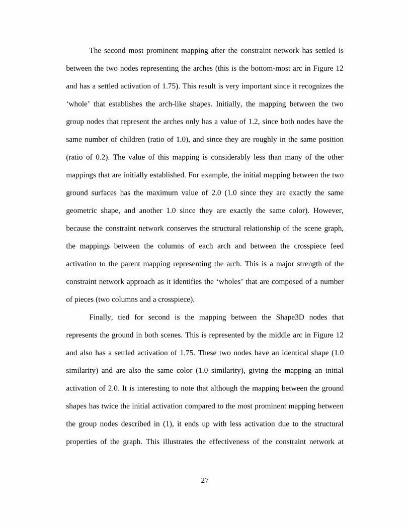
Figure 14 illustrates the output of DIVA’s visual analogy algorithm. The most prominent

mapping is between the head of the snowman and the head of the blockman, illustrated

by the bottom-most arc in Figure 14. This is not surprising since both head objects are

composed with a similar carrot-nose and coal-eyes. The second most-prominent

mappings is between the group nodes representing the overall snowman and the overall

blockman (illustrated by the middle arc in Figure 14). The third-most prominent mapping

is between the group node that collects the objects in the scene, illustrated by the top-

most arc in Figure 14.

30

Figure 14. Top 3 mappings output by DIVA's visual similarity algorithm for the

snowman-blockman example.

Dynamic Visual Similarity

Mapping dynamic visual analogies requires comparing the motions of the objects

in the source and target scenes. Pedone, Hummel and Holyoak (in press) investigated

the use of animated diagrams in analogical problem solving. As a target, they used the

much-investigated radiation problem, in which a way must be found to destroy a tumor

without injuring the flesh that surrounds it. One solution to the problem is to use a

number of radiation beams from all sides of the patient that converge on the tumor but are

not intense enough individually to harm the surrounding tissue. Pedone et al. found that

spontaneous retrieval and noticing the relevance of a problem analogous to the radiation

problem were increased markedly by animating displays representing converging forces.

Subjects were more successful using the convergence animations as a source analogy to

solve the tumor problems than were subjects given static diagrams or animated

divergence diagrams.

31

To test the applicability of our dynamic imagery program to complex visual

analogies, we produced VRML representations of the tumor problem and the fortress

problem, in which a general manages to destroy a fortress by dispersing his forces and

having them converge on the fortress. Holyoak and Thagard (1995) review the many

experiments that have been done using these problems. Unlike Pedone, Hummel and

Holyoak, who used an abstract diagram to represent a dynamic convergence solution, we

implemented dynamic versions of both the tumor and fortress problems using animated

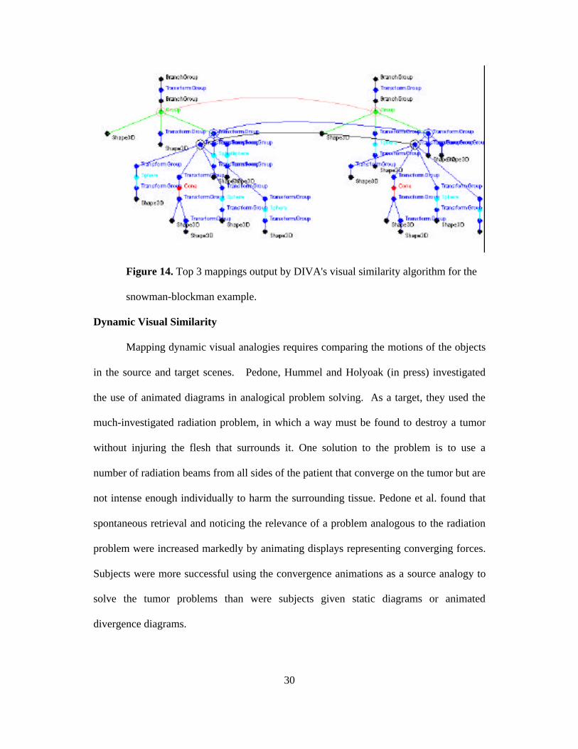
Java3D representations. Figure 15, a screen shot from the user interface, depicts the

tumor problem using a patient’s head and five rays converging towards it. Similarly,

Figure 16 depicts the fortress problem as a VRML representation of a castle surrounded

by soldiers who converge on it. Unfortunately, the printed figures do not show the

animation that occurs on the screen when the soldiers converge on the castle and the rays

converge on the head.

32

Figure 15. User interface showing the animated solution to the tumor

problem on the left. The right side contains the relevant part of the

semantic network.

33

Figure 16. User interface showing the animated representation of the castle

siege problem.

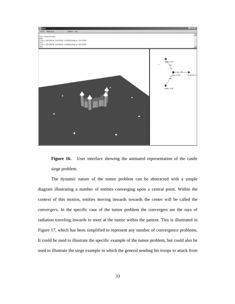
The dynamic nature of the tumor problem can be abstracted with a simple

diagram illustrating a number of entities converging upon a central point. Within the

context of this motion, entities moving inwards towards the center will be called the

convergers. In the specific case of the tumor problem the convergers are the rays of

radiation traveling inwards to meet at the tumor within the patient. This is illustrated in

Figure 17, which has been simplified to represent any number of convergence problems.

It could be used to illustrate the specific example of the tumor problem, but could also be

used to illustrate the siege example in which the general sending his troops to attack from

34

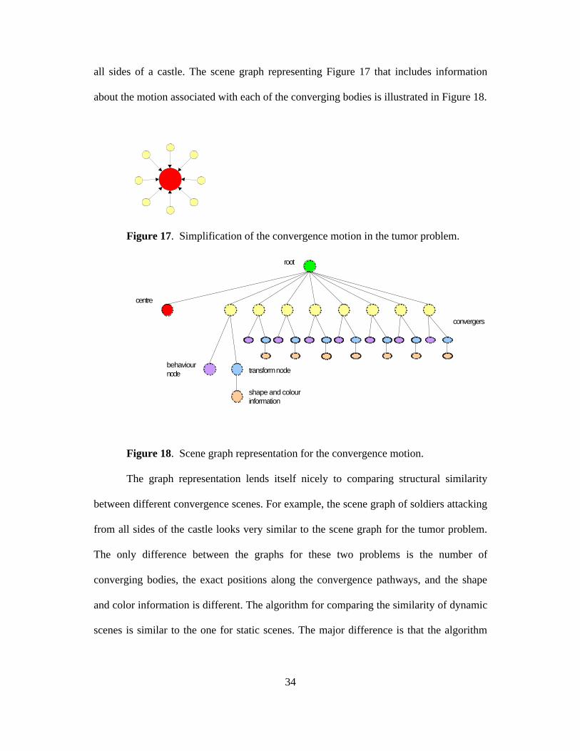
all sides of a castle. The scene graph representing Figure 17 that includes information

about the motion associated with each of the converging bodies is illustrated in Figure 18.

Figure 17. Simplification of the convergence motion in the tumor problem.

root

centre

behaviour node transform node

shape and colour information

convergers

Figure 18. Scene graph representation for the convergence motion.

The graph representation lends itself nicely to comparing structural similarity

between different convergence scenes. For example, the scene graph of soldiers attacking

from all sides of the castle looks very similar to the scene graph for the tumor problem.

The only difference between the graphs for these two problems is the number of

converging bodies, the exact positions along the convergence pathways, and the shape

and color information is different. The algorithm for comparing the similarity of dynamic

scenes is similar to the one for static scenes. The major difference is that the algorithm

35

for dynamic scenes considers all the behavior nodes present in each graph in an attempt

to identify a motion pattern such as convergence.

A general motion analysis, attempting to compare all the behavior nodes from one

scene graph with all the behavior nodes from another scene graph, is computationally

unfeasible because of the very large number of paths through 3-dimensional space that a

set of objects might take. In order to make comparison of two dynamic scenes

computational tractable, DIVA attempts to identify high-level patterns of motion,

searching through all the behavior nodes contained in each scene graph. Although the

current model focuses on convergence motion, work has also been done to identify

orbital and parallel motion patterns.

In the case of the tumor problem and castle siege, the algorithm that compares the

dynamic content of the two scenes starts by trying to classify high-level patterns of

motion, and finds that both scenes contain a convergence motion. In order to identify this

convergence motion, the algorithm looks at each behavior node within the scene graph

and tries to identify the direction of the pathway taken by that node as well as a common

point of convergence among two or more of the pathways.

Any system for dynamic imagery needs a mechanism for identifying important

patterns of motion such as convergence. According to Kosslyn (1994, p. 154), the brain

has a motion relations encoding subsystem that enables it to represent standard properties

of motion fields. Kosslyn and Koenig (1992, p. 78) state: “Computing motion relations

appears to be qualitatively distinct from computing the organization of portions of static

images, and distinct regions of the brain apparently encode motion.”

36

DIVA identifies the approximate point in space where most of the objects

converge as the convergence point. If more than one body is found in the scene moving

towards the convergence point, then the scene under consideration is classified as

containing a convergence motion. Note that the static object at the center of the scene

does not play any part in identifying the convergence motion. Whether the bodies are

moving in towards a central object, or whether they are just travelling in towards a

common point in space is irrelevant at this stage of the analysis. However, at a later stage

of the algorithm, the convergence point is used to establish a mapping between objects

that are being converged upon (eg. the head in the tumor problem and the castle in the

siege).

After identifying any motion pattern contained within two dynamic scenes, the

visual analogy algorithm proceeds in a similar fashion as explained for static visual

analogies, establishing mappings between the source and target graph. Similarity

comparisons between behavior nodes are based upon the motion pattern present in the

scenes. For example, in the case of the tumor problem and the castle siege, a ray of

radiation moving towards the front of the patient’s head would be considered visually

similar to a soldier moving towards the front of the castle.

The output of DIVA’s dynamic visual similarity algorithm for the tumor problem

and the castle siege is illustrated in Figure 19. The graph on the left represents the tumor

problem, and the graph on the right represents the castle siege. The most prominent

mapping is between the root node of the two graphs, indicating that the two dynamic

scenes are highly analogous (illustrated by the top-most arc on Figure 19). The second-

most prominent mapping is between the group nodes representing the head and the castle.

37

These two nodes are an important aspect of the analogy since they represent objects at the

center of the convergence motion (illustrated by the arc between the left-most branch of

the left graph and the left-most branch of the right graph). The other prominent mappings

output by DIVA’s dynamic visual similarity algorithm are between the converging

objects moving towards the center of their respective scenes at similar angles. If more

mappings were illustrated in Figure 19, all of the converging objects from the left graph

would have relatively strong mappings to a converging object in the right graph (these are

not shown since they add considerable clutter to the figure).

We speculate that the experimental results of Pedone et al. derive in part from the

subjects’ ability to detect convergence patterns by a means similar to DIVA’s. In

addition to common semantic associations and static visual similarities (color, shape,

structure etc..), the mind’s eye must consider high-level motion patterns when making

comparisons. The animated diagrams used in the experiments of Pedone et. al. provide

the necessary dynamic content that enables people to make the connection between the

convergence motion in the diagram and that required to solve the tumor problem. We

conjecture that people also make dynamic visual analogies based upon parallel and

orbital motion patterns.

38

Figure 19. Prominent mappings between the tumor problem and the castle siege

output by DIVA’s dynamic visual similarity algorithm.

Using scene graphs has enabled DIVA to become a much more general and

powerful model of visual analogies than previous accounts based on arrays (Conklin and

Glasgow, 1992; Thagard, Gochfeld, and Hardy, 1994). It is also representationally and

computationally richer than the Tabletop model of spatial analogies (French, 1995). In

particular, the use of behaviors in scene graphs can support a very high-level computation

of similarity between images involving motion. The examples described above show that

39

DIVA has the representational and computational power to model dynamic visual

analogies made by the human mind.

FUTURE DIRECTIONS

Our model of dynamic imagery can generate moving objects and simulate visual

analogies, but it captures only a small part of human capabilities for imagining objects in

motion. A richer model will need to add some knowledge of how objects in the world

interact physically with each other, and add more inferential mechanisms to enable it to

simulate problem solving, diagnosis, and thought experiments.

The current program lacks a physics model that would enable the behaviors of

different objects to connect with each other. For example, although the stick-man

illustrated in Figure 7 appears to be walking, there is no simulated frictional force

between the stick-man's feet and the ground, so that the stick-man would appear to

remain in the same position relative to the ground, always remaining in the same spot.

Similarly, when we imagine a ball travelling though the air, it rarely just hovers around at

a constant vertical level but is subject to our understanding of gravity. Hobson (1988)

gives the example of a dream in which a golf ball travels through the air and rebounds

from an object that it collides with. By itself, the scene graph used to represent visual

information is not subject to any natural laws. Hence a more powerful dynamic imagery

program would use physical laws to constrain motions produced through the behaviors

nodes present in a scene graph.

The addition of a physics model would improve a dynamic imagery program’s

ability to solve problems. It would be interesting, for example, to model how children

use visual information to build new structures out of LEGO blocks. A problem could be

40

posed using an image of a structure to be built, and a solution to the problem would

require a series of visual inferences about how the blocks could be combined to produce

the desired structure. It would also be desirable to simulate the role of imagery in

solving problems that require the generation of explanations. Shelley (1996) describes

numerous examples of abductive inference, the formation of explanatory hypotheses,

based on visual imagery. For example, anthropologists have explained the structure of

stone tools by visualizing them as being produced by controlled flaking using a stone

hammer. It would be natural to extend our model of dynamic imagery to simulate

hypothesis generation by visual reasoning. In addition, it should be possible to apply a

theory of dynamic imagery to the use of thought experiments and visual analogies in

scientific discoveries, as discussed by Brown (1991) and Nersessian (1992).

Finally, it would be desirable to provide a more neurologically realistic

representation of visual structure than is provided by the Java 3D scene graph. We

conjecture that the techniques that have been used to convert complex verbal

representations into distributed neural representations could also be used to produce

artificial-neural-network versions of our imagery program. Scene graphs could be

converted to complex vectors that preserve structural information (Smolensky, 1990;

Eliasmith and Thagard, forthcoming); or they could be translated into neuronal groups

that coordinate information by means of neural synchrony (Shastri and Ajjanagadde,

1993; Hummel and Holyoak, 1997). Either way, we would have steps toward a more

neurologically interesting model of dynamic imagery. A major challenge for both these

techniques, however, would be to find a means of representing motion.

41

CONCLUSION

In this paper, we have borrowed from computer graphics the idea of a scene graph

to suggest new structures and algorithms for modeling how people generate and use

dynamic visual images. Scene graphs are more flexible and inferentially powerful than

representations such as bitmaps and arrays that have been previously use to model mental

imagery. Most importantly, they provide a natural way to model how people can

generate images of objects in motion. Representation of physical objects involves not

only their static properties such as shape, color, and position, but also their behaviors.

Dynamic imagery is not like running a pre-compiled movie in the mind, but instead

requires a constructive process of combining the behaviors of different objects into novel

and flexible animations. Scene graph representations can support analogical mappings

between visual images, including ones that involve complex motions such as

convergence. We expect future work on dynamic imagery to extend our model to apply

to a wide range of cognitive processes, including problem solving, explanation, and

thought experiments.

Address for correspondence: Paul Thagard, Philosophy Department, University

of Waterloo, Waterloo, Ontario, Canada, N2L 3G1. E-mail: pthagard@uwaterloo.ca.

Acknowledgments: We are grateful to Rob Krajcarski and Micah Zarnke for

very helpful ideas and programming assistance. Thanks to Cameron Shelley and Keith

Holyoak for comments on an earlier draft. This research has been supported by the

Natural Sciences and Engineering Research Council of Canada.

42

REFERENCES

Anderson, J. R. (1983). The architecture of cognition. Cambridge, MA: Harvard University Press.

Brown, J. R. (1991). The laboratory of the mind. London: Routledge.

Chandrasekaran, B., Glasgow, J., & Narayanan, N. H. A. N. (Eds.). (1995). Diagrammatic reasoning:

Cognitive and computational perspectives. Cambridge, MA: AAAI Press/MIT Press.

Chella, A., Frixione, M., & Gaglo, S. (2000). Understanding dynamic scenes. Artificial Intelligence, 123,

89-132.

Conklin, D., & Glasgow, J. I. (1992). Spatial analogy and subsumption. In D. Sleeman & P. Edwards

(Eds.), Machine learning: Proceedings of the ninth international conference . San Mateo: Morgan

Kaufmann.

Eliasmith, C., & Thagard, P. (forthcoming). Integrating structure and meaning: A distributed model of

analogical mapping. Cognitive Science.

Falkenhainer, B., Forbus, K. D., & Gentner, D. (1989). The structure-mapping engine: Algorithms and

examples. Artificial Intelligence, 41, 1-63.

Forbus, K. (1995). Qualitative spatial reasoning: Framework and frontiers. In B. Chandrasekaran, J.

Glasgow, & N. H. A. N. Narayanan (Eds.), Diagrammatic reasoning: Cognitive and

computational perspectives . Cambridge, MA: AAAI Press / MIT Press.

French, R. (1995). Tabletop: An emergent, stochastic, computer model of analogy-making. Cambridge,

MA: MIT Press.

Funt, B. (1980). Problem solving with diagrammatic representations. Artificial Intelligence, 13, 201-230.

Gentner, D. (1983). Structure mapping: A theoretical framework for analogy. Cognitive Science, 7, 155-

170.

Glasgow, J. I., & Papadias, D. (1992). Computational imagery. Cognitive Science, 16, 355-394.

Hobson, J. A. (1988). The dreaming brain. New York: Basic Books.

Holyoak, K. J., & Thagard, P. (1989). Analogical mapping by constraint satisfaction. Cognitive Science,

13, 295-355.

43

Holyoak, K. J., & Thagard, P. (1995). Mental leaps: Analogy in creative thought. Cambridge, MA: MIT

Press/Bradford Books.

Hummel, J. E., & Holyoak, K. J. (1998). Distributed representations of structure: A theory of analogical

access and mapping. Psychological Review, 104, 427-466.

Kosslyn, S., & Koenig, O. (1992). Wet mind: The new cognitive neuroscience. New York: Free Press.

Kosslyn, S. M. (1994). Image and brain: The resolution of the imagery debate. Cambridge, MA: MIT

Press.

Larkin, J. H., & Simon, H. A. (1987). Why a diagram is (sometimes) worth ten thousand words. Cognitive

Science, 11, 65-100.

Nersessian, N. (1992). How do scientists think? Capturing the dynamics of conceptual change in science.

In R. Giere (Ed.), Cognitive Models of Science (Vol. vol. 15, pp. 3-44). Minneapolis: University of

Minnesota Press.

Pedone, R., Hummel, J. E., & Holyoak, K. J. (in press). The use of diagrams in analogical problem solving.

Memory and Cognition.

Pylyshyn, Z. (1984). Computation and cognition: Toward a foundation for cognitive science. Cambridge,

MA: MIT Press.

Shastri, L., & Ajjanagadde, V. (1993). From simple associations to systematic reasoning: A connectionist

representation of rules, variables, and dynamic bindings. Behavioral and Brain Sciences, 16, 417-

494.

Shelley, C. P. (1996). Visual abductive reasoning in archaeology. Philosophy of Science, 63, 278-301.

Smolensky, P. (1990). Tensor product variable binding and the representation of symbolic structures in

connectionist systems. Artificial Intelligence, 46, 159-217.

Tabachneck-Schuf, H. J. M., Leonardo, A. M., & Simon, H. A. (1997). CaMeRa: A computatioanal model

of multiple repesentations. Cognitive Science, 21, 305-350.

Thagard, P., Gochfeld, D., & Hardy, S. (1992). Visual analogical mapping, Proceedings of the Fourteenth

Annual Conference of the Cognitive Science Society (pp. 522-527). Hillsdale, NJ: Erlbaum.