dynamic curvature regulation accounts for the symmetric ... · pdf file(satir and matsuoka,...
TRANSCRIPT

For correspondence jonathon
howardyaleedu
daggerThese authors contributed
equally to this work
Competing interest See
page 19
Funding See page 19
Received 22 November 2015
Accepted 08 May 2016
Published 11 May 2016
Reviewing editor Raymond E
Goldstein University of
Cambridge United Kingdom
Copyright Sartori et al This
article is distributed under the
terms of the Creative Commons
Attribution License which
permits unrestricted use and
redistribution provided that the
original author and source are
credited
Dynamic curvature regulation accountsfor the symmetric and asymmetric beatsof Chlamydomonas flagellaPablo Sartori1dagger Veikko F Geyer2dagger Andre Scholich1 Frank Julicher1Jonathon Howard2
1Max Planck Institute for the Physics of Complex Systems Dresden Germany2Department of Molecular Biophysics and Biochemistry Yale University NewHaven United States
Abstract Cilia and flagella are model systems for studying how mechanical forces control
morphology The periodic bending motion of cilia and flagella is thought to arise from mechanical
feedback dynein motors generate sliding forces that bend the flagellum and bending leads to
deformations and stresses which feed back and regulate the motors Three alternative feedback
mechanisms have been proposed regulation by the sliding forces regulation by the curvature of
the flagellum and regulation by the normal forces that deform the cross-section of the flagellum In
this work we combined theoretical and experimental approaches to show that the curvature
control mechanism is the one that accords best with the bending waveforms of Chlamydomonas
flagella We make the surprising prediction that the motors respond to the time derivative of
curvature rather than curvature itself hinting at an adaptation mechanism controlling the flagellar
beat
DOI 107554eLife13258001
IntroductionCilia and flagella are long thin organelles whose oscillatory bending waves propel cells through flu-
ids and drive fluid flows across the surfaces of cells The internal motile structure the axoneme con-
tains nine doublet microtubules a central pair of single microtubules motor proteins of the
axonemal dynein family and a large number of additional structural and regulatory proteins
(Pazour et al 2005) The axonemal dyneins power the beat by generating sliding forces between
adjacent doublets (Summers and Gibbons 1971 Brokaw 1989) The sliding is then converted to
bending (Satir 1965) by constraints at the base of the axoneme (eg the basal body) andor along
the length of the axoneme (eg nexin links) (Brokaw 2009)
While the mechanism by which the sliding of a doublet is converted to bending is well estab-
lished it is not known how the activities of the dyneins are coordinated in space and time to produce
the periodic beating pattern of the axoneme For example bending the axoneme in one direction
requires higher dynein activity on one side of the axoneme than on the other if the activities are
equal then the forces will cancel and there will be no bending Therefore to alternatively bend in
one direction and then the other requires dynein activity to alternate between the two sides
(Satir and Matsuoka 1989) The switching of dynein activity is rapid taking place twice per beat
cycle and at rates above 100 times per second for Chlamydomonas The coordination required for
such rapidly alternating bending is thought to result from mechanical feedback the axonemal
dyneins generate forces that bend and deform the axoneme and the deformations in turn regulate
the dyneins Because of the geometry of the axoneme deformation leads to stresses and strains
Sartori et al eLife 20165e13258 DOI 107554eLife13258 1 of 26
RESEARCH ARTICLE
that have components in various directions (eg axial and radial) However which component (or
components) regulates the dyneins is not known
Three different but not mutually exclusive molecular mechanisms for dynein coordination have
been suggested in the literature (Figure 1D) (i) In the sliding control-mechanism the dyneins
behave as rsquoslip bondsrsquo they detach when subject to forces acting parallel to the long axis of the
microtubule doublets and that oppose sliding (Brokaw 1975 Julicher and Prost 1997
Camalet and Julicher 2000 Riedel-Kruse et al 2007) The build-up of sliding forces on one side
of the axoneme therefore induces detachment of the dyneins on the other side (and vice versa) the
two sides are antagonistic The resolution of this reciprocal inhibition or rsquotug of warrsquo is a catastrophic
detachment of dyneins on one side of the axoneme leading to an imbalance of sliding forces and
therefore to axonemal bending (ii) In the curvature-control mechanism the detachment of dynein is
regulated by doublet curvature (Morita and Shingyoji 2004 Brokaw 1972 Brokaw 2009) This
leads to a similar reciprocal inhibition because the sign of the curvature is opposite on opposite
sides of the axoneme (iii) In the normal-force control mechanism also called the geometric clutch
the detachment of dynein is regulated by transverse forces that act to separate adjacent doublets
when they are curved (Lindemann 1994b) Which if any of these mechanisms regulates the beating
of the axoneme is not known
In this work we developed a two-dimensional mathematical model of the axoneme that can
incorporate any or all of these different feedback mechanisms The model extends earlier models
(Camalet and Julicher 2000 Riedel-Kruse et al 2007) by including static curvature which gives
rise to asymmetric beats such as those of Chlamydomonas and of ciliated epithelial cells This model
is similar to a recent model (Bayly and Wilson 2014) We then tested the different feedback mecha-
nisms by comparing the predictions of the associated models with high spatial and temporal resolu-
tion measurements of the bending waveforms of isolated reactivated Chlamydomonas axonemes
(Hyams and Borisy 1975 Bessen et al 1980) We found that the curvature-control mechanism
accorded with experiments using both wild type cells which have an asymmetric beat and with
experiments using the mbo2 mutant which has a nearly symmetric beat By contrast the sliding
mechanism gave poor fits to both the wild type and mbo2 data and the normal-force mechanism
gave unsatisfactory fits to the mbo2 data
Theoretical modelTwo-dimensional model of the axonemeIn the two dimensional model we project the cross-section of the three-dimensional axoneme onto
a pair of filaments (Figure 1AB) The projection retains the key idea that motors on opposite sides
of the axoneme generate bends in opposite directions (Satir and Matsuoka 1989) The dyneins
that give rise to the principle bend (this corresponds to bends that lie on the outside of the curved
path along which an axoneme swims [Gibbons and Gibbons 1972] Figure 1AB green) which in
Chlamyodomonas has the same sign as the static curvature are combined to generate sliding in one
direction The dyneins that give rise to the reverse bend (Figure 1AB blue) are combined to gener-
ate sliding in the opposite direction
The two filaments have the same polarity (all motors move towards the base) and have combined
bending rigidity k They are assumed to be inextensible and held together by elastic elements that
maintain the filaments at a constant distance (a) from each other Although there is some evidence
that doublet separation is not constant (Lindemann and Mitchell 2007) our assumption simplifies
the theory while still allowing us to calculate the normal force in the elastic elements that keeps the
separation constant (Mukundan et al 2014) In our normal-force mechanism the motors are regu-
lated by the force rather than by the separation of the doublets as in Lindemann (1994a) However
if the normal force is small the separation is proportional to the force and the two models are
equivalent
The filaments are immersed in an aqueous fluid and experience drag forces arising from the fluid
viscosity The hydrodynamic forces are proportional to the velocity with friction coefficients n and
t (per unit length) for motion normal to and tangential to the axis of the filament The values of the
mechanical parameters are estimated in Appendix 5
The position of each point on the filament pair is specified at each time by the vector r seth THORN a func-
tion of the arc-length s along the centerline between the filaments Calculating the tangent vector
Sartori et al eLife 20165e13258 DOI 107554eLife13258 2 of 26
Research article Biophysics and structural biology Cell biology
as t seth THORN frac14 _r seth THORN where dots denote arc-length derivatives allows us to define the tangent angle seth THORN
with respect to the horizontal axis of the laboratory frame The tangent angle characterizes the
shape of the filament For a given filament shape the pair of filaments will have a local sliding dis-
placement D seth THORN We assume that the filaments are incompressible though they can support tension
along their centerline For incompressible filaments sliding is linearly related to the tangent angle
via
D seth THORN frac14 Dbthorn a seth THORN 0eth THORNfrac12 (1)
where Db frac14 D 0eth THORN is the basal sliding (Figure 1C) The sign convention is defined in Figure 10 and
Appendix 4
C
D sliding control normal force controlcurvature control
detach load
force
+ + +
A
reverse bend
principal bend
11
11
bending plane
dynein
nexin
cross-links
1
2
3 4
5
7
8
9
6
z
y x
y
xz
3
9
4
8
B
base
tip
(-)
(+)
detach detach
projection
two 90deg
rotations
normal
force
Figure 1 Two-dimensional model of the axoneme and mechanisms of dynein regulation (A) Cross-section of an
axoneme as seen from the basal end looking towards the distal tip The numbering of the doublets follows the
convenstion for Chlamydomonas (Hoops and Witman 1983) The green dyneins bend the axoneme such that the
center of curvature is to the right (B) The projection of the cross section onto two filaments to form the two-
dimensional model The green and blue motors bend the filament pair in opposite directions (C) Two-
dimensional model of the axoneme as seen in the bending plane xy The two filaments are constrained to have
spacing a The point at arc-length s has position vector r (relative to the origin) tangent vector t normal vector n
and tangent angle with respect to the horizontal axis of the lab-frame xy Dyneins on the upper filament (green)
have microtubule-binding domains (MTBs denoted by filled circles) that walk along the lower filament towards the
base and produce a (tensile) force density thornf on the lower filament This force slides the lower filament towards
the distal end The dyneins on the opposite filament (blue) create sliding (and bending) forces in the opposite
direction The local sliding displacement is given by D and the sliding at the base is Db The sign convention is
defined in Figure 10 and Appendix 4 The springs between the filaments oppose filament separation by the
normal force f The spring and dashpot at the base consitute the basal compliance with stiffness kb and friction
coefficient b (D) Schematic of dynein regulation mechanisms In curvature control the dynein MTB detaches due
to an increase in curvature In sliding control detachment is enhanced by a tangential loading force and in normal
force control the normal force which tends to separate the filaments enhances detachment Signs indicate
doublet polarity
DOI 107554eLife13258002
Sartori et al eLife 20165e13258 DOI 107554eLife13258 3 of 26
Research article Biophysics and structural biology Cell biology
To compare the observed periodic beats to those predicted by the model we write the tangent
angle as a sum of Fourier modes
s teth THORN frac14X
yen
nfrac14yen
n seth THORNexp inteth THORN (2)
where is the angular frequency of the beat (=2p is the beat frequency in cycles per second) t is
time i is the imaginary unit and n are the modes (indexed by n) The modes are complex-valued
functions of arc-length that represent the amplitude and phase of the beat waveforms They satisfy
n frac14 n to keep the angle real ( represents the complex conjugate) For each value of ngt1 there is
an associated equation of motion We refer to nfrac14 0 as the static mode which corresponds to the
time-averaged shape We refer to nfrac14 1 as the fundamental mode which corresponds to the
dynamic shape at the beat frequency The static and fundamental modes are the only ones consid-
ered in this work In this case we can write s teth THORN frac14 0 seth THORNthorn j 1 seth THORN j sin tthornf seth THORNfrac12 where j 1 seth THORN j is
the amplitude of the fundamental mode and f seth THORN is the phase (arg ) We use the complex formula-
tion because it simplifies the theory whose goal is to make predictions for j 1 seth THORN j and f seth THORN to com-
pare to the experimental data (eg Figure 3iindashiii) The same modal decomposition can be done for
all other parameters that depend on time including the sliding displacement D seth THORN the basal sliding
Db the sliding force between the filaments f and the tension t in the centerline of the filaments
Force balance in the axonemeThe shape of the axoneme depends on the balance between the mechanical forces (from the motors
and the elastic elements) and the hydrodynamic forces The mechanical force is the derivative (with
respect to the position vector r) of the work functional U (Appendix 1 Equation 11) which depends
on the bending rigidity of the doublets the stiffness of the cross linkers motor forces and the shape
of the filament This force is balanced by the hydrodynamic force from the fluid which is propor-
tional to the velocity (qtr) of the axoneme at each point P qtr frac14 dU=dr where P is the friction
matrix (Lauga and Powers 2009) For a slender body at low Reynolds number the friction matrix is
P frac14 nnnthorn ttt where n seth THORN a unit vector normal to the tangent vector t seth THORN (Figure 1C) Force bal-
ance yields non-linear equations of motion (Equations 14ndash16 in Appendix 1 also see Sartori 2015)
We then derive the static solution corresponding to mode n frac14 0 and the periodic solution at the
beat frequency corresponding to mode n frac14 1
Static modeIf the motor forces do not change with time then the axoneme will not move and the hydrodynamic
forces are zero causing the tension in the axoneme to be zero The static mode of the filament pair
can be calculated from the static force-balance equation
k _ 0 seth THORN frac14 aF0 seth THORN F seth THORN frac14
Z L
s
f s0eth THORNds0 (3)
where _ 0 seth THORN the arc-length derivative of the tangle angle is the curvature of the static mode and
F0 seth THORN is the static mode of the integrated motor force (Appendix 1 Equation 19) The static mode is
the time-averaged shape which in Chlamydomonas axonemes has approximately constant curva-
ture all along the length and as a result _ 0 seth THORNraquoC0 (Geyer et al 2016 Eshel and Brokaw 1987)
(see Results) In our theoretical analysis we therefore ignore deviations from constant curvature
Such deviations are not expected to significantly affect the conclusions of this work because we
found that the static curvature had little effect on the dynamics (the wild type and mbo2 axonemes
have similar beats see Results) According to the static force-balance equation bending an axo-
neme into a shape with constant curvature requires the integrated motor force to be independent of
arc-length which in turn requires the motor forces be concentrated near the distal end
(Mukundan et al 2014) We therefore approximate the static component of the motor force den-
sity by
f0 frac14d sLeth THORNkC0=a (4)
Sartori et al eLife 20165e13258 DOI 107554eLife13258 4 of 26
Research article Biophysics and structural biology Cell biology
where d is the Dirac delta function and the minus sign ensures that a positive dynein force produces
a negative curvature in accord with our sign convention (Appendix 4)
Dynamic modeTo obtain the equation of motion at the beat frequency (ie the n frac14 1 dynamic mode) we substitute
the modal expansions of the tangent angle (Equation 2) the motor force and the tension into the
non-linear dynamic equations and keep only the terms at the fundamental frequency (n frac14 1)
in 1 frac14k euroeuro1 thorn aeurof1 thorn 1thorn n=tfrac12 C0 _t1 thorn n=teth THORNC20ethk
euro 1 af1THORN
n=teth THORNeurot1 C20t1 frac14 1thorn n=teth THORNfrac12 C0 k euro_ 1 a_f1
(5)
(Appendix 1 Equations 14ndash16 Appendix 2 Equation 21) Associated with these equations are
boundary conditions specifying the tangent angle (and its spatial derivatives) and the tension at the
basal and distal ends (Appendix 2 Equation 20) The boundary conditions for a freely swimming
axoneme correspond to no external forces or torques acting at the ends
Equation 5 generalizes previous models of symmetrically beating axonemes (Machin 1958 Rie-
del-Kruse et al 2007 Camalet and Julicher 2000 in which the static curvature (C0) and the axial
tension (t1) are zero For C0 6frac14 0 new terms appear and the system of equations is of order six rather
than four in the symmetric case The magnitude of the new terms can be estimated by considering
the plane-wave approximation in which 1 seth THORN frac14 exp 2pis=leth THORN with lraquo L the wavelength The plane
wave is sinusoidal s teth THORN frac14 sin t 2ps=leth THORN Though the plane wave is only an approximation to the
(i)
10 microm
500 nm
500 nm
B
10 microm
(i) (ii)
(i) (ii)
002 006 01
0
2
4
6
Time t (s)
Ta
ng
en
t a
ng
le
(ra
d)
002 006 01
0
2
4
6
Time t (s)T
an
ge
nt
an
gle
(ra
d)
(m
rad)
(n
m)
Arc-length s ( microm)0 5 10
0
10
20
0
20
40
60
(m
rad)
(iii)
(iii)
(iv)
(v)
(iv)
(v)
A wild type
mbo2 mutant
0 5 10
0 5 10
0 5 100
10
20
0
20
40
60
Arc-length s ( microm)
Arc-length s ( microm)
Arc-length s ( microm)
(n
m)
Figure 2 High precision tracking of isolated reactivated axonemes Panel A corresponds to Chlamydomonas wild type axonenes panel B to mbo2
mutant axonemes (A) (i) Inverted phase-contrast image of a wild type axoneme The orange curve represents the tracked centerline The points depict
the basal end (red) the distal end (green) and the center position (black) of the axoneme The yellow line depicts the trajectory of the basal end which
is the leading end during swimming (Geyer 2012) (ii) Same image as in Ai magnified around the center region The tangent angle s teth THORN is defined
with respect to the lab frame (iii) Tangent angle at three different arc-length positions (depicted in Ai) as a function of time The linearly increasing
tangent angle corresponds to a counter-clockwise rotation of the axoneme during swimming Mean uncertainty measured over 1000 adjacent frames of
the position dr y (iv) (the dr x error gives a similar result) and the tangent angle d in (v) (B) is analogous to (A) but for mbo2 mutant axonemes
DOI 107554eLife13258003
Sartori et al eLife 20165e13258 DOI 107554eLife13258 5 of 26
Research article Biophysics and structural biology Cell biology
shape and does not satisfy the boundary conditions (eg the curvature at the distal end of an axo-
neme is always zero) it is nevertheless useful for calculating approximate values of parameters For
example the fourth term on the right hand side of the upper equation is of order n=teth THORNC20k 2p=leth THORN2
and is in phase with the first term which is of order k 2p=leth THORN4 For Chlamydomonas axonemes l ~ L
and C0 ~p=L and since n=t raquo 2 (Appendix 5) the ratio of these terms is ~ 05 A similar reasoning
shows that the third term is in anti-phase and its contribution is of order ~ 1 This shows that the
new terms which enter through the asymmetry can not be neglected a priori Thus for the large
observed asymmetry of the Chlamydomonas axoneme we expect that there is coupling between
the n frac14 0 and n frac14 1 modes significantly modifying the dynamics of the beating axoneme As we will
see the static curvature C0 has little effect in the curvature-control model but has a large effect in
the normal-force model
Equation 5 shows how an oscillatory active sliding force f s teth THORN frac14 f1 seth THORNeit thorn f 1 seth THORNeit can produce
dynamic bending of the axoneme (with appropriate parameter and boundary conditions) To see
this note that the upper equation can be rearranged to provide an expression for t1 in terms of 1
and f1 (and their derivatives) This expression can then be substituted into the lower equation to
provide a relationship between 1 and f1 so that if f1 is known 1 can be calculated A trivial exam-
ple is when f1 frac14 0 in which case the only solutions are 1 frac14 0 and t1 frac14 0 If f1 is non zero the equa-
tion may have non-trivial solutions corresponding to bending oscillations
Three mechanisms of motor controlWe now build the three molecular mechanisms of motor control into the two-dimensional model of
the axoneme Equation 5 shows that an oscillating sliding force can produce a dynamic beating pat-
tern However we do not expect the motor proteins themselves to be the oscillators because oscil-
lations have never been observed in single-molecule recordings (but see Shingyoji et al 1998)
Rather we expect that the sliding forces generated by the dyneins are regulated directly or indi-
rectly by the shape of the axoneme Such regulation constitutes mechanical feedback If we have an
expression for how the motor force depends on the tangent angle (and its derivatives) this can be
substituted into the equation of motion which can then be solved (using the boundary conditions)
to predict bending waveforms
The most general linear expression for the dependence of the motor force on sliding curvature
and normal force is
fn seth THORN frac14 neth THORNDn seth THORNthornb neth THORN
n seth THORNthorng neth THORNfn seth THORN (6)
where n 0 is the mode index eth THORN b eth THORN and g eth THORN are complex frequency-dependent coefficients
describing how the motor force responds to sliding curvature and normal forces respectively The
coefficients depend on the molecular properties of the dyneins such as their density along the dou-
blets their force-velocity curves and the sensitivity of their unbinding on load force on curvature or
on normal force they also depend on the elastic and viscous resistance to sliding between the dou-
blets (Camalet and Julicher 2000 Riedel-Kruse et al 2007) If the density of motors and the
mechanical properties are independent of arc-length then the coefficients will also be independent
of the arc-length Though light and electron microscopy studies have shown that there are longitudi-
nal variations in dynein isoforms and dynein density (Yagi et al 2009 Bui et al 2012) we ignore
these variations in the present work Such variation could be included in more elaborate models
(eg Riedel-Kruse et al 2007) The coefficients are complex because in general the force could
depend on the instantaneous value of the parameter (the real part) and or on the rate of change of
the parameter (the imaginary part) To see this suppose that the force depends on the sliding dis-
placement (D) and the sliding velocity (qtD) Then f s teth THORN frac14 kD s teth THORNthorn qtD s teth THORN and in the Fourier repre-
sentation f1 seth THORN frac14 kthorn ieth THORND1 seth THORN so frac14 kthorn i Finally the coefficients will in general depend on
frequency through delays caused by the finite detachment times The response coefficients are the
generalization to active motors of the linear response coefficient of a passive system For example
the basal force of the axoneme Fb frac14 F 0eth THORN is described by Fb frac14 kbDb thorn bqtDb where kb is the basal
stiffness and b is the basal damping coefficient Thus the fundamental mode of the basal force is
given by Fb1 frac14 b eth THORNDb1 with basal impedance b eth THORN frac14 kbthorn ib
Sartori et al eLife 20165e13258 DOI 107554eLife13258 6 of 26
Research article Biophysics and structural biology Cell biology
In our model the response coefficients are small at zero frequency This is because the observed
nearly constant static curvature implies that the static component of the force (f0) is approximately
zero all along the length except near the distal end of the axoneme (see Equation 4)
The motor force equation (Equation 6) together with the equation of motion (Equation 5) define
a dynamical system which can become unstable and produce spontaneous oscillations (Julicher and
Prost 1997 Camalet et al 1999) At the critical point these oscillations are periodic and we only
retain the fundamental mode (n frac14 1) These critical-point oscillations constitute the predicted beat
waveforms of our two-dimensional model (see last paragraph of Appendix 1)
Normal-force controlWe conclude the theory section with a discussion of the normal force Unlike the sliding control and
curvature control mechanisms in which the motor force depends linearly on the tangent angle (and
its derivatives) the feedback in the normal-force model is non-linear This is because the normal
force is the product of the integrated sliding force and the curvature f frac14 F _ (Appendix 1
0 200 400Frequency (Hz)
10-6
10-4
10-2
Arc-lengths0 5 10
-3
-2
-1
0
00
04
08
12
-6
-4
0
-2
Arc-lengths0 5 10
Arc-lengths0 5 10
(i) (ii) (iii) (iv)
0 200 400Frequency (Hz)
10-6
10-4
10-2
0 5 10-3
-2
-1
00
04
08
12
-6
-4
0
-2
0 5 10 0 5 10
0
data reconstruction data reconstruction
A
B
C D
(i) (ii) (iii) (iv)
wild type
mbo2
wild type mbo2
Phase
Mean P
ow
er
s
2
Arc-lengths Arc-lengths Arc-lengths
Phase
Mean P
ow
er
s
2
Figure 3 Fourier decomposition of the beat Panel A shows the Fourier decomposition of the waveform of wild
type axonemes panel B the decomposition of the mbo2 axoneme waveform (A) (i) Power spectrum of the
tangent angle averaged over arc-length The fundamental mode (n frac14 1) and three higher harmonics (n frac14 2 3 4) are
labeled (ii) Angular representation of the static (n frac14 0) mode as a function of arc-length The approximately
constant slope indicates that the static curvature is close to constant
0 frac14 C0 (iii) The amplitude and phase
(argument) of the fundamental mode are shown in iii and iv respectively The approximately linear decrease in
phase indicates steady wave propagation The data of a representative axoneme is highlighted in the panels iindashiv
with error bars indicating the standard error of the mean calculated by hexadecimation (B) Equivalent plots to (A)
for mbo2 axonemes (C) Beat shapes of one representative beat cycle of the wild type axoneme highlighted in
panel A (left panel data) and shapes reconstructed from the superposition of the static and fundamental modes
neglecting all higher harmonics The progression of shapes through the beat cycle is represented by the rainbow
color code (see inset) (D) Same as (C) for an mbo2 mutant axoneme
DOI 107554eLife13258004
Sartori et al eLife 20165e13258 DOI 107554eLife13258 7 of 26
Research article Biophysics and structural biology Cell biology
Equation 16) both of which depend on arc-length However under the assumption that the static
curvature is constant 0
frac14 C0 the normal force can be linearized simplifying the solution of the
dynamical equations Expanding F and _ into their static and fundamental Fourier modes and using
the static force balance aF0 frac14 kC0 we obtain the following expression for the fundamental mode of
the normal force
f1 frac14C0 F1 thornk _ 1=a
(7)
where F1 is the fundamental mode of the integrated sliding force (Appendix 1 Equation 19) Thus
the force is linear in the curvature and the integrated motor force Equation 7 vanishes for symmet-
ric beats in which the static curvature is zero (C0 frac14 0THORN The important implication is that for symmetric
beats there is no reciprocal inhibition across the axoneme unlike sliding and curvature control This
is related to the property that static bends produce normal forces that always tends to separate fila-
ments independent of the sign of the bend (Mukundan et al 2014) Thus the static curvature
C0 6frac14 0 of the Chlamydomonas beat opens a way for regulation by normal forces something impos-
sible in symmetrically beating cilia of which sperm is an approximate example (Riedel-Kruse et al
2007)
Results
Quantification of the beat of wild type and mbo2 ciliaTo test the different mechanisms of beat regulation we measured the flagellar beating waveforms in
wild type and mbo2 axonemes with high temporal and spatial precision (Materials and methods and
Figure 2i-ii) We tracked trajectories of 20 points along the arc-length of the axoneme as a function
of time over up to 200 beat cycles (Figure 2iii) Copies of the movies and the extracted tangent
angles are available (see Sartori et al 2016) The uncertainty of the position in xy space was
raquo 5 nm and the uncertainty in the tangent angle was raquo20 mrad (Figure 2iv-v) The latter corre-
sponds to a sliding displacement between adjacent doublet microtubules of only 13 nm
Because the beat of Chlamydomonas is periodic in time it is convenient to decompose the tan-
gent angle s teth THORN into Fourier modes n (Equation 2) Before doing so we note that wild type Chla-
mydomonas axonemes swim counterclockwise in circles at a slow angular rotation speed
rot raquo 30 rad=s (Figure 2Aiiii) While the effect of this rotation is small for a single beat it becomes
large for a long time series Before performing the Fourier decomposition we therefore subtracted
rott from the tangent angle s teth THORN (for simplicity we use the same notation for s teth THORN and
s teth THORN rott) The power spectrum of the tangent angle (averaged over the flagellar length) shows
clear peaks at harmonics of its fundamental frequency (Figure 3Ai) Because the peak at the funda-
mental frequency n frac14 1eth ) accounts for 90 of the total power we neglected the higher harmonics
(n = 234 ) for reconstructing the flagellar shape We found that using just the n frac14 0 and n frac14 1
modes gave excellent reconstitutions of both the wild type and mbo2 beats (Figure 3CndashD) Thus
the static and fundamental modes provide a good description of the beats
The amplitude of the static mode (n frac14 0) and the amplitude and phase of the fundamental mode
(n frac14 1) are shown in (Figure 3iindashiv) The main difference between the wild type and mutant axo-
nemes comes from the static mode 0 (Figure 3ii Eshel and Brokaw 1987 Geyer et al 2016)
For wild type axonemes 0 decreased approximately linearly over arc-length This corresponds to
an approximately constant static curvature raquo 025 radmm and indicates that the time-averaged
shape is close to a semi-circular arc of radius raquo 4 mm The static curvature of wild type axonemes
leads to the highly asymmetric waveform In contrast mbo2 mutant axonemes have a small static
mode with a curvature raquo0025 radmm corresponding to an approximately symmetric waveform
In comparison to the large differences in the static mode between wild type and mutant axo-
nemes the fundamental modes 1 are similar The amplitude of 1 is roughly constant and has a
characteristic dip in the middle (Figure 3iii) The argument of 1 which determines the phase of the
wave decreases at a roughly constant rate in both cases (Figure 3iv) indicating that the beat is a
traveling wave Because the total phase shift is about 2p the wavelength of the beat is approxi-
mately equal to the length of the axoneme Thus both wild type and mutant axonemes have
Sartori et al eLife 20165e13258 DOI 107554eLife13258 8 of 26
Research article Biophysics and structural biology Cell biology
approximately sinusoidal dynamic beats whose amplitudes dip in the middle of the axoneme and
whose wavelengths are approximately equal to their lengths
Motor regulation in the axoneme experiment versus theoryTo gain insight into how molecular motors in the axoneme are controlled we compared experimen-
tal beating patterns to those calculated from theory In the sliding-control model the motor force
depends only on sliding through the sliding coefficient frac14 0 thorn i00 The single and double primes
denote real and imaginary parts 0 and i00 describe the dependence of force on the sliding dis-
placement and the sliding velocity They are the elastic and damping components of the sliding
response respectively Because the response must be active for oscillations to occur we have
0 00 0 (Machin 1958) In the sliding-control model the motor force is independent of curvature
and normal forces so the curvature coefficient (b) and the normal force coefficient (g) were set to
zero In the curvature-control model the curvature coefficient is non-zero (b 6frac14 0) In addition we
allow the possibility that the motors have a passive response to sliding (corresponding to elastic
resistance to shear between adjacent doublets at the beat frequency) so that 0gt0 The motors are
not regulated by normal force (g frac14 0) In the normal-force model g 6frac14 0 We again allow for the pos-
sibility that the motors have a passive response to sliding (0gt0) The motors are not regulated by
curvature (b frac14 0THORN) Note that for backward traveling waves the signs of b0b00 and g0 g00 change but
those of 0 00 do not
Sliding control Curvature control Normal force control
00 02 04 06 08 10
-10
-05
00
05
10
Arc-length sL
R2 052 R
2 095 R2 095
02 04 06 08 10
-10
-05
00
05
10
Arc-length sL02 04 06 08 10
-10
-05
00
05
10
Arc-length sL00 00
Sliding control Curvature control Normal force controlR2 067 R
2 097 R2 097
02 04 06 08 10
-10
-05
00
05
10
Arc-length sL0002 04 06 08 10
-10
-05
00
05
10
Arc-length sL0002 04 06 08 10
-10
-05
00
05
10
Arc-length sL
Re(Ψ
1)
ampIm
(Ψ1)
00
wild type mbo2 mutant
theory experiment theory experiment
Re(Ψ
1)
ampIm
(Ψ1)
Re(Ψ
1)
ampIm
(Ψ1)
Re(Ψ
1)
ampIm
(Ψ1)
Re(Ψ
1)
ampIm
(Ψ1)
Re(Ψ
1)
ampIm
(Ψ1)
C D
B
A wild type
mbo2 mutant=
= = =
==
Figure 4 Comparison of theoretical and experimental beating patterns (A) Comparison of the theoretical (lines)
and experimental (dots) beating patterns of a typical wild type axoneme The real and imaginary part of the first
mode of the tangent angle 1 seth THORN is plotted for beats resulting from sliding control curvature control and normal
force control (B) Analogous to (A) for mbo2 Note that here also curvature control and normal force control
provide good agreement but not sliding control (C) and (D) Theoretical and experimental shape reconstruction in
position space for the wild type and mbo2 beats under curvature control
DOI 107554eLife13258005
Sartori et al eLife 20165e13258 DOI 107554eLife13258 9 of 26
Research article Biophysics and structural biology Cell biology
We tested the three motor models by adjusting the appropriate response coefficients together
with the basal stiffness (kb) and the basal damping coefficient (b) to obtain the closest fit of their
predictions to the dynamic mode The fitting procedure is described in Appendix 3 using the
mechanical parameters described in Appendix 5 The result of a typical fit for wild type axonemes is
shown in Figure 4A The real and imaginary parts of the fundamental mode 1ethsTHORN ndash corresponding
to the cosine and sine components of the waveforms ndash agree well with the data in the cases of curva-
ture control and normal-force control but not for sliding control In the latter case the real and
imaginary parts of the predicted mode are in anti-phase (Figure 4A left panel) corresponding to a
standing wave and contradicting the observed propagating wave The xy representation of the beat-
ing pattern predicted by the curvature-control model agrees well with the experimental beating pat-
tern reconstructed from the static and fundamental modes (Figure 4C) The good agreement
reinforces the conclusion from Figure 4A that the curvature control model accords with the experi-
mental data for wild type axonemes Similar good agreement for wild type axonemes was found
with the normal-force model Table 1 summarizes average parameters resulting from the fits to data
from 9 wild type axonemes
We compared the theory to the dynamic modes measured from the mbo2 mutant where the
static curvature is reduced by at least one order of magnitude compared to wild type beats (Fig-
ure 3) The results were similar to those of wild type (Figure 4B) sliding control could not produce
bend propagation while curvature and normal force control were in good agreement with the
experimental data The parameters obtained from the fit of mbo2 beats are given in Table 2 We
also fit the model to the wild type waveforms in which the static curvature had been subtracted A
good fit to the curvature control model was obtained but not to the sliding control model Thus
the fundamental mode was well fit by the curvature and normal-force models but not sliding control
Regulation of the beat by slidingThe sliding-control model provides a poor fit to the observed beating patterns This can be under-
stood using three different but related arguments First in the plane-wave approximation 1 frac14
expeth2pis=lTHORN the wavelength satisfies
in=kfrac14eth2p=lTHORN4 eth2p=lTHORN2a2=k (8)
Because the equation is unchanged when ll there are solutions for propagation from base to
tip (lgt0) and for propagation from tip to base (llt0) These two waves superimpose to form a stand-
ing wave inconsistent with the observed traveling wave
The second argument is that in the limit of very short axonemes (L 0) sliding control predicts
that there will only be standing waves irrespective of whether the boundary conditions are
Table 1 Parameters for beat generation in wild type axonemes
Sliding control Curvature control Normal-force control
Coefficient of determination R2 eth THORN 49 4 95 1 95 1
Sliding coefficient 0 00 nN m2eth THORN 122 3011 01 198 33 0 132 36 0
Curvature coefficient b0b00 nNeth THORN 0 065 04 0
Normal-force coefficient g0 g00 0 0 012 005 20 02
Basal impedance 0b
00b nN m1eth THORN 424 07 2800 6900 422 12 22 07 80 115 13000 34000
Basal sliding (0th mode) Db0 ethnmTHORN 41 41 36 12 144 196
Basal sliding (1st mode) jDb1j ethnmTHORN 23 19 22 5 12 11
The values reported are mean and standard deviation calculated from 9 axonemes The average static curvature is C0 frac14 0232 0009 m1 the
length L frac14 117 04 m and the frequency frac14 427 19 rads (68 Hz) Note that for curvature controlled beats using the value of b and an estimate
curvature of 01 rad=m results in a sliding force of raquo 700 pN=m Since the motor density of an active half of the axoneme is raquo 500m1 the individual
motor force is ~ 1 pN For the case of normal force control the sliding force generated by the motors is of the order of the normal force that they expe-
rience since jgjraquo 2
DOI 107554eLife13258006
Sartori et al eLife 20165e13258 DOI 107554eLife13258 10 of 26
Research article Biophysics and structural biology Cell biology
symmetric or not (Camalet and Julicher 2000) Chlamydomonas axonemes are short in the sense
that are much shorter than the critical length
lsquofrac14 2pk
n
1=4
(9)
which is 26m using the Chlamydomonas parameters (Appendix 5) Based on this limit we only
expect standing waves
The third argument is a generalization of the second Though short Chlamydomonas axonemes
have a non-zero length We therefore computed the bend propagation speed according to
v frac14R L
0j 1j
2qs arg 1ds Using the amplitude and phase of the experimental data for Chlamydomonas
j 1j ~ 068 (Figure 2Aiii and (Geyer et al 2016) and arg 1 frac14 2ps=L (Figure 2Aiv) the bend prop-
agation speed is raquo 3 By contrast the bend propagation speed predicted by the sliding control
model is only 0005 3 Thus the sliding-control model predicts a bend propagation speed much
lower than observed
That the low bend propagation speed is due to the short length of the Chlamydomonas axoneme
can be appreciated by plotting the predicted speed (normalized by the measured speed of Chlamy-
domons) against length L (normalized by the critical length) Figure 5A shows that at short lengths
such as for Chlamydomonas the wave propagation speed is very slow whereas for lengths above
the critical length such as for sperm the propagation speed is high
Thus there are several arguments for why sliding control does not work for the short flagella of
Chlamydomonas
Regulation of the beat by normal forcesThe normal-force model provides a good fit to the beating patterns of wild type and mbo2 axo-
nemes However there are two related arguments against the normal-force model First despite the
similarities in the dynamics of the beats of wild type and mbo2 axonemes (Figure 3iiindashiv) the normal
force model requires very different values for the response coefficient g for wild type and mbo2
axonemes (Tables 1 and 2) Second the normal-force model applied to mbo2 requires large differ-
ences in g from axoneme to axoneme despite the similarity in the dynamics among the axonemes
(Figure 3Biiindashiv) To understand why this is the case we plotted g as a function of the inverse of the
curvature The two are strongly correlated jgj jC0j1(Figure 6A) This correlation follows from
Equation 7 which predicts that the dynamic component of the normal force is linearly proportional
to the static curvature C0 In other words the normal-force model requires there be static curvature
if the static curvature were exactly equal to zero then the model would break down However the
static curvature in mbo2 axonemes is so small as few as 3 degrees over the length of the axoneme
that it is likely to be residual and of no significance It is therefore puzzling why the key control
parameter would depend so strongly on a residual property By contrast the curvature-control
Table 2 Parameters for beat generation in mbo2 mutant axonemes
Sliding control Curvature control Normal-force control
Coefficient of determination R2 ethTHORN 72 5 95 1 96 1
Sliding coefficient 0 00 ethnNm2THORN 150 1004 01 174 25 0 105 43 0
Curvature coefficient b0b00 ethpNTHORN 0 0066 04 0
Normal-force coefficient g0 g00 0 0 152 152 32 25
Basal impedance 0b
00b ethnNm1THORN 306 141 16 07 21 2 23 17 23 03 136 60
Basal sliding (0th mode) Db0 ethnmTHORN 6 6 73 44 64 40
Basal sliding (1st mode) jDb1j ethnmTHORN 51 10 60 11 77 28
Values are averages and standard deviations for 9 axonemes The static curvature was C0 frac14 00276 0005 m1 the length L frac14 92 03 m and the
frequency frac14 176 44 rads (28 Hz) Note that the values of g in normal force control are very spread out and compared to the wild type fits In fact
in one case we obtained g raquo 80 indicating that motors must amplify the normal force they sense by almost two orders of magnitude The values for cur-
vature control are very similar to those of wild type fits
DOI 107554eLife13258007
Sartori et al eLife 20165e13258 DOI 107554eLife13258 11 of 26
Research article Biophysics and structural biology Cell biology
coefficient b is similar for wild type and mbo2 axonemes and is independent of the static curvature
(Figure 6B) Thus we conclude that normal force is not a plausible parameter for controlling the cili-
ary beat
Regulation of the beat by curvatureThe curvature control model provides a good fit to the experimental data for both wild type and
mbo2 axonemes (Figure 4A and B middle panel) Initially we fitted the data using non-zero values
for both the sliding control parameters (0 00) and for both the curvature control parameters (b0
b00) We found that the best fit values of 00 and b0 were not significantly different from zero Further-
more the quality of the fits were as good when we set both to zero We therefore took 00 = b0 frac14 0
(Tables 1 and 2) We present an argument in the Discussion for why these two parameters are
expected to be zero Thus the curvature control model is specified by just two free parameters the
sliding elasticity between doublet microtubules at the beat frequency eth0THORN and the rate of change of
axonemal curvature (b00) (note that the parameters 0b and 00
b which characterize the stiffness and
viscosity at the base respectively are determined once 0 and b00 are specified in order to satisfy the
boundary conditions [final paragraph of Appendix 2])
The average values of 0 and b00 varied little between wild type and mbo2 mutant axonemes
(compare the third column of Table 1 with that of Table 2 see also Figure 6B) This accords with
the observation that there is little difference in the dynamical properties of the beat between wild
type and mbo2 axonemes Furthermore the standard deviations of 0 and b00 are small indicating
that there is little variation from axoneme to axoneme Thus the tight distribution of values of the
parameters in the model reflects the similarity in the observed shapes in different axonemes In other
words 0 and b00 are well constrained by the experimental data
To understand what aspects of the experimental data specify these two parameters we per-
formed a sensitivity analysis on 0 and b00 In Figure 7A we show a density map of the mean square
distance R2 between the theoretical waveforms and a reference experimental beating pattern as a
function of 0 and b00 The red ellipse delimits a region of good fit in which R2gt090 This region
closely coincides with the region where 0b and 00
b are both positive which is delimited by the central
pair of black lines This is important because negative values of the basal parameters imply an active
process at the base which would result in a whip-like motion of the axoneme as noted by Machin
(Machin 1958) From the shapes of beating spermatozoa Machin argued against such an active
base
We systematically varied 0 and b00 parallel and perpendicular to the long axis of the ellipse Mov-
ing perpendicular into the region of active base indeed results in whip-like beats with a larger ampli-
tude at the base (Figure 7B blue circles) This argues against a basal whip-like driving of the
Waveform 2Waveform 1B C
Waveform 1
Waveform 2
Chlamydomonas Bull sperm
A
-06
Norm
aliz
ed w
ave s
peed v
-03
0
03
06
Normalized axoneme length
13 13
02 0205 10 15 20
Figure 5 The role of length in sliding-regulated beats (A) Wave speed versus relative length of the first two
unstable waveforms of a freely swimming axoneme regulated by sliding For short lengths in the range of
Chlamydomonas the modes lose directionality and become standing waves Long axonemes have directional
waves that can travel either forward as in waveform 1or backwards as in waveform 2 (B) Two examples of
waveform 1 for long (top) and short (bottom) axonemes Note that the short axonemes have standing waves See
(Sartori 2015) for more details (C) Beating patterns of waveform 2 for a long (top) and short (bottom) axonemes
In B and C arrows denote direction of wave propagation
DOI 107554eLife13258008
Sartori et al eLife 20165e13258 DOI 107554eLife13258 12 of 26
Research article Biophysics and structural biology Cell biology
motion of Chlamydomonas axonemes Moving parallel affects the amplitude of the beat with the
middle-dip becoming more or less prominent (Figure 7B green circles) Thus the arc-length depen-
dence of the amplitude of the fundamental mode constrains the value of the response coefficients
and the sign of the basal response
To better understand the cell-to-cell variability we plotted data from all the axonemes in the
eth0b00THORN space (Figure 8A) Points scatter mainly along the long axis of the ellipse where there is a
large region of small shape variation We consistently saw a shift perpendicular to the long axis
between the wild type and mbo2 axonemes This variation correlates with the difference in normal-
ized lengths between wild type and mutant axonemes (Figure 8B) suggesting a possible depen-
dence of the response coefficients on length andor frequency
A striking difference between the wild type and mbo2 axonemes is that the curve-fitting indicates
that the basal stiffness in the mutant is about 20-fold smaller than in the wild type (Table 1 and
2) This softening at the base is associated with a larger basal sliding in the mutant Whether this dif-
ference causes the difference in beat frequency (the mutant beats more slowly) or whether it is a
consequence of the shorter lengths of the mutant axonemes (Figure 8C) will require additional
study
DiscussionIn this work we imaged isolated axonemes of Chlamydomonas with high spatial and temporal resolu-
tion We decomposed the beating patterns into Fourier modes and compared the fundamental
mode which is the dominant dynamic mode with theoretical predictions of three motor control
mechanisms built into a two-dimensional model of the axoneme (Figure 1) The sliding control
model provided a poor fit to the experimental data We argued that the reason for this is that sliding
control cannot produce wave propagation for axonemes as short as those of Chlamydomonas (Fig-
ure 5) While the normal-force model (also termed the geometric clutch model) provided good fits
to the experimental data it relies on the presence of static curvature (Bayly and Wilson 2015)
which varies greatly between the mbo2 and wild type axonemes As a result of this large difference
in static curvature the control parameters in this model had to be varied over a wide range to fit the
data from the different axonemes (Figure 6) Because the waveforms of mbo2 and wild type axo-
nemes have similar dynamic characteristics such variation in the control parameter seems implausi-
ble and we therefore argue against regulation by normal forces in the two-dimensional model
Finally the curvature-control model provided a good fit to the experimental data with similar param-
eters for mbo2 and wild type axonemes Thus we conclude that only the curvature-control model is
fully consistent with our experimental data
A potential caveat of these conclusions is that the model used here is two-dimensional Impor-
tantly in order to simplify the geometry the model only contains one pair of filaments While this
captures the essential features of the sliding control and curvature control models it oversimplifies
the normal-force model because in the three-dimensional axoneme there are radial and transverse
forces acting on the doublets as the axoneme bends Yet the two-dimensional model does not
Radius of curvature
Norm
al fo
rce
coeffic
ient
0 50 100 150 2000
40
80
Radius of curvature0 50 100 150 200
Curv
atu
re c
oeffic
ient
nN
0
4
8
mbo2
wild-type
A B
mbo2
wild-type
Figure 6 Scaling of response coefficients with static curvature (A) Because the normal force f1 is proportional to
the static curvature C0 the normal force response coefficient g is inversely proportional to the curvature Red
symbols are mbo2 and green symbols are wild type (B) The curvature control response coefficient b00 is
independent of the static curvature and remains constant even for a fifty-fold change in static curvature
DOI 107554eLife13258009
Sartori et al eLife 20165e13258 DOI 107554eLife13258 13 of 26
Research article Biophysics and structural biology Cell biology
distinguish between them To bridge this gap in
other work (Sartori et al 2015) we developed
a full three-dimensional model of the axoneme
to calculate the radial and transverse stresses
The three-dimensional model shows that even
when there is a static curvature (without twist)
normal (transverse) forces are not antagonistic
across the centerline and therefore cannot serve
as a control parameter for motors
Relation with past workEarlier results showed that sliding control can
account for the beating patterns of sperm
(Camalet and Julicher 2000 Riedel-
Kruse et al 2007 Brokaw 1975) This is con-
sistent with the present results because the bull
sperm axoneme is approximately five times lon-
ger than the Chlamydomonas axoneme and we
have shown that sliding control can lead to bend
propagation in long axonemes (Figure 5 and
see Brokaw 2005) Thus it is possible that dif-
ferent control mechanisms operate in different
cilia and flagella with sliding control being used
in longer axonemes and curvature control being
used in shorter ones However we do note that
curvature control models can account for the
bull sperm data (Riedel-Kruse et al 2007) as
well as data from other sperm (Brokaw 2002
Brokaw 1985 Bayly and Wilson 2015) so
there is no strong morphological evidence favor-
ing either sliding or curvature control in sperm The normal-force model produces beating patterns
that resemble those of sperm (Lindemann 1994b Bayly and Wilson 2015 Bayly and Wilson
2014) However these models rely on there being an asymmetry which is small and variable in
sperm arguing against normal-force control Thus the curvature control model unlike the other two
models robustly describes symmetric and asymmetric beats in short and long axonemes and could
serve as a rsquouniversalrsquo regulator of flagellar mechanics
Dynamic curvature control as a mechanism for motor regulationAn unexpected feature of our curvature control model is that the motor force depends only on the
time derivative of the curvature This follows from the fact that the curvature response function b has
no real part (Table 1 and 2 see Theoretical Model section) Such a model is fundamentally different
from the current views of curvature control in which motors are thought to respond to instantaneous
curvature (Brokaw 1972 Brokaw 2002 Brokaw 2009) and not to its time derivative
While motors can respond to time derivatives of sliding displacement through their force-velocity
relation it is hard to understand how a similar mechanism could apply to curvature One possibility
is that there is a curvature adaptation system analogous to that of sensory systems like the signaling
pathway of bacterial chemotaxis (Macnab and Koshland 1972 Yi et al 2000 Shimizu et al
2010) In an adaptation mechanism curvature (or motor activity) would be rsquorememberedrsquo and the
average curvature (or motor activity) over past times would in turn down-regulate the activity of the
motors on a long time-scale Such regulation could occur for example via phosphorylation sites in
the dynein regulatory complex or the radial spokes (Witman 2009 Smith and Yang 2004
Porter and Sale 2000) Just as methylation of the chemoreceptors of bacteria modifies their ligand
affinity phosphorylation of regulatory elements within the axoneme could modify the motor sensitiv-
ity to curvature over times long compared to the period of the beat
04 08 12 16
08
12
098
091
096
Arc-length sL00 05 10
00
04
08
12
Arc-length sL00 05 10
Arc-length sL00 05 10
B
A
Norm
aliz
ed
Normalized
Figure 7 Phase space of curvature control (A) Heat
map of the mean-square distance R2 between the
theoretical and a reference experimental beat as a
function of the sliding response coefficient 0 and the
curvature response coefficient b00 The ellipsoid delimits
the region with R2 frac14 090 Each pair of nearby black
lines delimits a region with a passive base Moving
along the long axis (green circles) affects the amplitude
dip in the midpoint of the axonemem left panel in (B)
Moving along the short axis towards the region of
active base results in waveforms with a large amplitude
at the base (blue and red circles) central and right
panels in B The axis in A is normalized by the
reference fit such that eth0 frac14 1b00 frac14 1THORN corresponds to
the highest value of R2
DOI 107554eLife13258010
Sartori et al eLife 20165e13258 DOI 107554eLife13258 14 of 26
Research article Biophysics and structural biology Cell biology
The molecular mechanisms underlying curva-
ture sensing are unknown A difficulty with
dyneins directly sensing microtubule curvature is
that the strain in a curved microtubule (radius of
curvature 4 mm) is very small ( raquo 1) correspond-
ing to a sub-angstrom strain in a tubulin dimer
Such a small strain would be difficult for an indi-
vidual dynein microtubule-binding domain to
detect though this difficulty could be circum-
vented if dynein binding were cooperative as
found for microtubule curvature-sensing by dou-
blecortin (Bechstedt et al 2014) On the other
hand indirect curvature-sensing mechanisms
that rely on the central pair pathway (Wit-
man 2009) are difficult to reconcile with
mutants missing the central pair and radial
spokes (Yagi and Kamiya 2000 Frey et al
1997) Thus our findings highlight the question
of how curvature might be sensed in the
axoneme
Independence of static anddynamic waveform componentsOur dynamic curvature control model adds to
the view that dynamic and static components of
the beat are regulated independently The prob-
lem with models in which dynein activity is regu-
lated by the instantaneous value of the curvature
is that both the static and dynamic components
of the beat would contribute to regulation and
hence the dynamic component of the waveform
would be highly dependent on the static compo-
nent (Sartori 2015) Yet the dynamic beats of wild type and mbo2 are similar as also noted in
(Eshel and Brokaw 1987) Our dynamic curvature control model provides a solution to this problem
because static curvature is rsquoadaptedrsquo away We now bring together several lines of evidence sup-
porting the notion that the static and dynamic modes are separable in their origin and in their affect
on the beat
1 Dynamic and static components of the beat can exist independently of each other This is evi-denced by the existence of bent non-motile cilia at low ATP concentrations on the one handas well as symmetrically beating mutants on the other (Geyer et al 2016)
2 The waveform of mbo2 has a fundamental dynamic mode similar to that of wild type Figure 3Aiii and Biii However the static mode is absent in the former Figure 3 Aii and Bii The samealso holds for the two beating modes of the uniflagellar mutant (Eshel and Brokaw 1987)Thus altering the static mode of Chlamydomonas has little effect on the dynamic mode
3 The dynamic motor response coefficients are largely independent of the asymmetry and verysimilar for mbo2 and wild type axonemes (Figure 6 A)
If the dynamic and static modes are indeed independently controlled the dynamic motor
response is robust to changes in the asymmetry This has important biological implications power
generation (the beat) and steering (the asymmetry) can be independently controlled so that the
swimming direction can be adjusted without having to alter the motor properties We note how-
ever that the molecular origin of asymmetry is not known nor is the mechanism by which the mbo2
mutation leads to symmetric beats (see Geyer et al 2016 for a discussion of possible mechanisms)
04 08 16
Dis
tan
ce
to
axis
08
12
024 032 040 048
005
010
000024 032 040 048
100
10-1
10-2
015
12
mbo2
wild-type
Axoneme lengthAxoneme length
No
rma
lize
d
Normalized
Figure 8 Axonemal variability in phase space (A)
Circles represent values obtained from fits for each of
the axonemes green corresponds to wild type and red
to mbo2 In the background we have the same heat
map as in Figure 7 Note that mbo2 points lie away
from wild type circles in the direction of the short axis
of the ellipse All values are normalized by those of the
reference fit used also to normalize the heat map axis
(B) The distance of the circles to the long axis of all fits
shows a clear correlation with normalized axonemal
length Note also that mbo2 axonemes are
systematically shorter than wild type axonemes (C) The
basal compliance (b) also correlates with the
normalized length resulting in a high value for wild
type axonemes which are longer The values are
normalized by the value for a reference axoneme
DOI 107554eLife13258011
Sartori et al eLife 20165e13258 DOI 107554eLife13258 15 of 26
Research article Biophysics and structural biology Cell biology
Phase of motor activity during the beatOur work predicts how the timing of motor activity drives the bending of the axoneme during the
beat The simplest way to understand the spatio-temporal relationship between motor force f and
axoneme curvature _ is to use the plane-wave approximation eths tTHORN frac14 sinetht 2ps=lTHORN where is
the frequency in radians per second and l is the wavelength in microns Differentiation with respect
to time t leads to a phase advance by p=2 (90 degrees or a quarter of a cycle) This can be appreci-
ated by noting that the cosine function (the derivative of sine) reaches its maximum before the sine
function (in the complex representation expfrac12ietht 2ps=lTHORN differentiation with respect to time leads
to multiplication by i which is equivalent to a phase lead of p=2 since i frac14 expethip=2THORN) For a traveling
wave moving from base to tip (ie moving in the direction of increasing arc-length s) the wave-
length is positive and differentiation with respect to arc-length leads to a phase delay by p=2 This
can be appreciated by noting that cosethsTHORN the derivative of sinethsTHORN reaches its maximum after the
original function Thus time derivatives lead and spatial derivatives lag
Using these differentiation rules we can represent the phase relations between the axonemal
parameters on a phase plot (Figure 9A) For the reference phase we use the sliding displacement
D or the tangent angle which are proportional to each other in the plane-wave approximation
ethD frac14 a THORN we define them (arbitrarily) to zero degrees (compass bearing east E) The sliding velocity
qtD has a phase lead of p=2 (ie compass bearing N on the phase plot) The curvature the derivative
of tangent angle with respect to arc-length qs frac14 _ has a phase delay of p=2 (ie S on the phase
plot) The key parameter is motor force which in the curvature-control model is
f1 frac14 0D1 thorn ib00qs 1 raquo frac12a
0 thorn b00eth2p=lTHORN 1 Using the parameters for wild type axonemes in Table 1
the sliding stiffness 0 frac14 thorn20 nN=m2 and the dynamic curvature coefficient b00 frac14 65 nN together
with a frac14 0066m and l frac14 L frac14 117m we find that the absolute magnitude of the first term in the
square bracket is smaller than the second term which is negative Thus in the plane-wave approxi-
mation the sign of the force is opposite that of the tangent angle and so the motor force is out of
phase with the tangent angle and sliding (compass bearing W)
An exact calculation shows that the phases predicted by the curvature control model are similar
to those of the plane-wave approximation Thus the tangent angle (Figure 9A gray arrow) lags
slightly behind the sliding displacement (Figure 9A black arrow E) due to the delay associated with
the basal compliances Furthermore the curvature (Figure 9A blue arrow) lags the plane-wave cur-
vature (S) due to the basal compliance and because the wavelength has a small imaginary compo-
nent Likewise the motor force (Figure 9A red arrow) lags slightly behind the plane-wave force (W)
Thus the exact theory shows that curvature leads the motor force by approximately one quarter of a
cycle and is nearly out of phase with the sliding displacement The time series for the various param-
eters are plotted in Figure 9B
From these phase relations we can use the curvature-control model to predict the activity of the
motors in relation to the curvature of the axoneme These predictions can then be compared to
structural studies such as cryo-electon microscopy Because the motor force lags the curvature
(Figure 9B) the motor force is in phase with the spatial derivative of the curvature Thus the motor
force is positive in the region marked green in Figure 9D and negative in the blue region In other
words the motors whose bases are statically attached to the upper filament are actively interacting
with the lower filament with their microtubule-binding domains to drive the bend that will develop
at this place as the wave travels towards the distal tip The motors with opposite polarity (ie on the
opposite side of the axoneme) will be active proximal to the bend Such a relative phase of the
motor activity with respect to curvature is a consequence of the dynamic curvature mechanism the
force that generates the curvature (Figure 9C green) is activated by the rate of change in curvature
with a sign (b00 lt 0) consistent with our sign convention Note that if these predictions are to be com-
pared to experiments then the static curvature needs to be subtracted
Efficiency and energeticsOur finding that the motor force is nearly out of phase with the sliding displacement (and tangent
angle) shows that the Chlamydomonas flagellum does not operate close to optimal efficiency The
maximally efficient phase was defined as the phase of the motors that maximized the swimming
speed while minimizing the elastic and viscous dissipation (ie minimizing energy consumption)
(Machin 1958) Machin showed that for a plane wave the optimum occurs when the phase of the
Sartori et al eLife 20165e13258 DOI 107554eLife13258 16 of 26
Research article Biophysics and structural biology Cell biology
motors is at 225 degrees (compass bearing SW) considerably different from our predicted motor
phase which is lt180 degrees Thus unlike sperm which Machin calculated to be close to the opti-
mum the short cilia of Chlamydomonas deviate considerably from optimum efficiency
The reason that Chlamydomonas deviates from optimum efficiency is that the elastic dissipation
dominates over the viscous dissipation Elastic dissipation arises from the straightening of the bent
axoneme and the loss of the associated bending energy (for an asymmetric beat like that of Chlamy-
domonas in which the static and dynamic modes have approximately equal amplitudes the elastic
loss is almost twice as great as that for a symmetric beat) Indeed in the plane wave approximation
the ratio of the viscous to elastic dissipation is p=2eth THORN L=lsquoeth THORN4 1 This inequality which was noted
recently (Chen et al 2015) holds for Chlamydomonas because Chlamydomonas axonemes are
shorter than the critical length (lsquo) By contrast the inequality is 1 for the much longer mammalian
sperm axonemes (and raquo 1 for sea-urchin sperm) Note that the dependence of the critical length
(Equation 9) on the mechanical parameters - drag coefficient and bending rigidity - is very weak due
to the 14 power dependence As a result even if the bending rigidity were five times smaller than
our estimate (Pelle et al 2009) our argument would still be valid Thus the short length of Chlamy-
domonas axonemes has important implications for the energetics of the flagellar beat
The reasoning behind the relatively small viscous dissipation also allows us to understand why the
curvature mechanism is sensitive to the rate of change of curvature rather than the instantaneous
value Equation 5 for a symmetric plane wave (C0 frac14 0) regulated by curvature (using
f1 frac14 a thornb _ frac14 a thorn ib 2p=l) gives
Phase
A B
Time
Recovery stroke
C D
Forc
e (
)
lead lag
Breast stroke
travelling wave
Figure 9 Phase delays and active force distribution on the axoneme (A) Polar representation of the phases of
sliding D curvature _ normal force f and the sliding force f for a beating axoneme regulated by curvature For a
plane wave eths tTHORN frac14 sin etht 2ps=lTHORN a time derivative rotates the phase counter-clockwise through p=2 radians
while a spatial derivative rotates the phase clockwise by p=2 radians Deviations from the compass points (E S W
N) are due to deviations of the axonemal beat from a plane wave Machinrsquos prediction for an optimum flagellum is
shown as the red dashed line (B) Time evolution of the quantities in A(C) Illustration of the local sliding force for a
shape of a symmetrically beating axoneme (eg mbo2) The regions of motor activity on the upper and lower
filament are highlighted in blue and green respectively (D) Asymmetrically beating wild type axoneme with two
shapes highlighted during the breast and recovery strokes The arrows represent direction of motion of the
axoneme and the colored patches represent the local sliding force on the respective filaments (see panel C and
Figure 1)
DOI 107554eLife13258012
Sartori et al eLife 20165e13258 DOI 107554eLife13258 17 of 26
Research article Biophysics and structural biology Cell biology
nthorn a200eth2p=lTHORN2 ab0eth2p=lTHORN3 frac14 0
keth2p=lTHORN4 thorn a20eth2p=lTHORN2thorn ab00eth2p=lTHORN3 frac14 0(10)
The upper line of Equation 10 shows that b0 produces an active motor force to counter the vis-
cous dissipation due to the fluid and the inter-filament sliding If the fluid damping coefficient is
small then we can have solutions with 00 frac14 b0 raquo0 Furthermore if the sliding response coefficient is
small (000 small) then j b0=b00 j raquo ethl=lTHORN4 1 showing that the dynamic curvature response domi-
nates over the instantaneous response Thus the dynamic curvature dependence is a consequence
of the viscous forces being small compared to the elastic forces
Summary and outlookWe finish the discussion by noting that the short length of Chlamydomonas flagella relative to the
critical length lsquo frac14 2pethk=nTHORN1=4 is key to understanding not just the energetics but also the mecha-
nism of motor control Indeed it was the shortness of the axonemes that implied that the sliding
control model only generated a standing wave and so could not recapitulate the observed traveling
wave Furthermore it was the shortness that gave rise to the imaginary curvature control coefficient
leading to the dynamic curvature-control mechanism In addition the shortness implies that the vis-
cous dissipation is small compared to the elastic dissipation These conclusions are robust because
the power of 14 in the expression for the critical length makes it quite insensitive to the parameter
values The long length of sperm leads to quantitatively different properties (eg the viscous and
elastic energies are of similar magnitude leading to efficient motion as argued by Machin) Whether
the long axonemes use the same dynamic curvature-control mechanism as short axonemes will
require further study
Materials and methods
Preparation and reactivation of axonemesAxonemes from Chlamydomonas reinhardtii wild type cells (CC-125 wild type mt+ 137c RP Levine
via NW Gillham 1968) and mutant cells that move backwards only (CC-2377 mbo2 mt- David
Luck Rockefeller University May 1989) were purified and reactivated The procedures described in
the following are detailed in Alper et al (2013)
Chemicals were purchased from Sigma Aldrich MO if not stated otherwise In brief cells were
grown in TAP+P medium under conditions of illumination (2x75 W fluorescent bulb) and air bub-
bling at 24˚C over the course of 2 days to a final density of 106 cellsml Flagella were isolated using
dibucaine then purified on a 25 sucrose cushion and demembranated in HMDEK (30 mM HEPES-
KOH 5 mM MgSO4 1 mM DTT 1 mM EGTA 50 mM potassium acetate pH 74) augmented with
1 (vv) Igpal and 02 mM Pefabloc SC The membrane-free axonemes were resuspended in HMDEK
plus 1 (wv) polyethylene glycol (molecular weight 20 kDa) 30 sucrose 02 mM Pefabloc and
stored at 80˚C Prior to reactivation axonemes were thawed at room temperature then kept on
ice Thawed axonemes were used for up to 2 hr
Base
(-)
Tip
(+)
y
x
Figure 10 Sign convention for motors that step towards the base See text for details
DOI 107554eLife13258013
Sartori et al eLife 20165e13258 DOI 107554eLife13258 18 of 26
Research article Biophysics and structural biology Cell biology
Reactivation was performed in flow chambers of depth 100 mm built from easy-cleaned glass and
double-sided sticky tape Thawed axonemes were diluted in HMDEKP reactivation buffer containing
1 mM ATP and an ATP-regeneration system (5 unitsml creatine kinase 6 mM creatine phosphate)
used to maintain the ATP concentration The axoneme dilution was infused into a glass chamber
which was blocked using casein solution (from bovine milk 2 mgmL) for 10 min and then sealed
with vacuum grease Prior to imaging the sample was equilibrated on the microscope for 5 min and
data was collected for a maximum time of 20 min
Imaging of axonemesThe reactivated axonemes were imaged by either phase constrast microscopy (wild type axonemes)
or darkfield microscopy (mbo2 axonemes) Phase contrast microscopy was set up on an inverted
Zeiss Axiovert S100-TV microscope using a Zeiss 63 Plan-Apochromat NA 14 Phase3 oil lens in
combination with a 16 tube lens and a Zeiss oil condenser (NA 14) Data were acquired using a
EoSens 3CL CMOS highspeed camera The effective pixel size was 139 nmpixel Darkfield micros-
copy was set up on an inverted Zeiss Axiovert 200 microscope using a Zeiss 63 Plan achromat NA
iris 07ndash14 oil lens in combination with an 125 tube lens and a Zeiss oil darkfield condenser (NA
14) Data were acquired using a pco dmaxS highspeed camera In both cases the illumination was
performed using a Sola light engine with a 455 LP filter Movies of up to 3000 frames were recorded
at a frame rate of 1000 fps The sample temperature was kept constant at 24˚C using an objective
heater (Chromaphor)
High precision tracking of isolated axonemesTo track the axoneme in each movie frame with nm precision the Matlab-based software tool
FIESTA was used (Ruhnow et al 2011) Prior to tracking movies were background subtracted to
remove static inhomogeneities arising from uneven illumination and dirt particles The background
image contained the mean intensity in each pixel calculated over the entire movie This procedure
increased the signal-to-noise ratio by a factor of 3 (Alper et al 2013) Phase-contrast images were
inverted darkfield images were tracked directly
The tracking algorithm FIESTA uses manual thresholding to determine the filament skeleton
which is then divided into square segments During tracking the filament position in each segment
is determined independently For tracking a segment size of 733 nm (approximately 5x5 pixels) was
used corresponding to the following program settings a full width at half maximum of 750 nm and
a ldquoreduced box size for tracking especially curved filamentsrdquo of 30 Along the arc-length of each
filament 20 equally spaced segments were fitted using two-dimensional Gaussian functions Two
examples of spline-fitted shapes are presented in Figure 2Ai and Bi superimposed on the image
The mean localization uncertainty of the center position of each of these segments was about 5 nm
(Figure 2Aiv and Biv) For localization of the ends the program uses a different fitting function
resulting in an increased uncertainty
Additional information
Competing interestsFJ Reviewing editor eLife The other authors declare that no competing interests exist
Funding
Funder Author
Yale University Jonathon Howard
Max-Planck-Gesellschaft Frank Julicher
The funders had no role in study design data collection and interpretation or thedecision to submit the work for publication
Sartori et al eLife 20165e13258 DOI 107554eLife13258 19 of 26
Research article Biophysics and structural biology Cell biology
Author contributions
PS FJ JH Participated in conception and design Analysis and interpretation of data Drafted and
revised the article VFG Participated in conception and design Analysis and interpretation of data
Drafted and revised the article Acquired data AS Participated in analysis and interpretation of data
Author ORCIDs
Frank Julicher httporcidorg0000-0003-4731-9185
Jonathon Howard httporcidorg0000-0003-0086-1196
Additional files
Major datasets
The following dataset was generated
Author(s) Year Dataset title Dataset URL
Database licenseand accessibilityinformation
Sartori P Geyer VFScholich A JulicherF Howard J
2016 Data from Dynamic curvatureregulation accounts for thesymmetric and asymmetric beats ofChlamydomonas flagella
httpdxdoiorg105061dryad0529j
Available at DryadDigital Repositoryunder a CC0 PublicDomain Dedication
ReferencesAlper J Geyer V Mukundan V Howard J 2013 Reconstitution of flagellar sliding Methods in Enzymology 524343ndash369 doi 101016B978-0-12-397945-200019-6
Bayly PV Wilson KS 2014 Equations of interdoublet separation during flagella motion reveal mechanisms ofwave propagation and instability Biophysical Journal 1071756ndash1772 doi 101016jbpj201407064
Bayly PV Wilson KS 2015 Analysis of unstable modes distinguishes mathematical models of flagellar motionJournal of the Royal Society Interface 1220150124 doi 101098rsif20150124
Bechstedt S Lu K Brouhard GJ 2014 Doublecortin recognizes the longitudinal curvature of the microtubuleend and lattice Current Biology 242366ndash2375 doi 101016jcub201408039
Bessen M Fay RB Witman GB 1980 Calcium control of waveform in isolated flagellar axonemes ofchlamydomonas The Journal of Cell Biology 86446ndash455 doi 101083jcb862446
Brokaw C 1989 Direct measurements of sliding between outer doublet microtubules in swimming spermflagella Science 2431593ndash1596 doi 101126science2928796
Brokaw CJ 1972 Computer simulation of flagellar movement I demonstration of stable bend propagation andbend initiation by the sliding filament model Biophysical Journal 12564ndash586 doi 101016S0006-3495(72)86104-6
Brokaw CJ 1975 Molecular mechanism for oscillation in flagella and muscle Proceedings of the NationalAcademy of Sciences of the United states of America 723102ndash3106 doi 101073pnas7283102
Brokaw CJ 1985 Computer simulation of flagellar movement VI simple curvature-controlled models areincompletely specified Biophysical Journal 48633ndash642 doi 101016S0006-3495(85)83819-4
Brokaw CJ 2002 Computer simulation of flagellar movement VIII Coordination of dynein by local curvaturecontrol can generate helical bending waves Cell Motility and the Cytoskeleton 53103ndash124 doi 101002cm10067
Brokaw CJ 2005 Computer simulation of flagellar movement IX oscillation and symmetry breaking in a modelfor short flagella and nodal cilia Cell Motility and the Cytoskeleton 6035ndash47 doi 101002cm20046
Brokaw CJ 2009 Thinking about flagellar oscillation Cell Motility and the Cytoskeleton 66425ndash436 doi 101002cm20313
Bui KH Yagi T Yamamoto R Kamiya R Ishikawa T 2012 Polarity and asymmetry in the arrangement of dyneinand related structures in the chlamydomonas axoneme The Journal of Cell Biology 198913ndash925 doi 101083jcb201201120
Camalet S Julicher F Prost J 1999 Self-organized beating and swimming of internally driven filaments PhysicalReview Letters 821590ndash1593 doi 101103PhysRevLett821590
Camalet S Julicher F 2000 Generic aspects of axonemal beating New Journal of Physics 224 doi 1010881367-263021324
Chen DT Heymann M Fraden S Nicastro D Dogic Z 2015 ATP consumption of eukaryotic flagella measured ata single-cell level Biophysical Journal 1092562ndash2573 doi 101016jbpj201511003
Cross MC Hohenberg PC 1993 Pattern formation outside of equilibrium Reviews of Modern Physics 65851ndash1112 doi 101103RevModPhys65851
Eshel D Brokaw CJ 1987 New evidence for a biased baseline mechanism for calcium-regulated asymmetry offlagellar bending Cell Motility and the Cytoskeleton 7160ndash168 doi 101002cm970070208
Sartori et al eLife 20165e13258 DOI 107554eLife13258 20 of 26
Research article Biophysics and structural biology Cell biology
Frey E Brokaw CJ Omoto CK 1997 Reactivation at low ATP distinguishes among classes of paralyzed flagellamutants Cell Motility and the Cytoskeleton 3891ndash99 doi 101002(SICI)1097-0169(1997)381lt91AID-CM8gt30CO2-K
Friedrich BM Riedel-Kruse IH Howard J Julicher F 2010 High-precision tracking of sperm swimming finestructure provides strong test of resistive force theory The Journal of Experimental Biology 2131226ndash1234doi 101242jeb039800
Geyer VF 2012 Characterization of the Flagellar Beat of the Single Cell Green Alga Chlamydomonas ReinhardtiiQucosa httpnbn-resolvingdeurnnbndebsz14-qucosa-130922
Geyer VF Sartori P Friedrich BM Julicher F Howard J 2016 Independent control of the static and dynamiccomponents of the chlamydomonas flagellar beat Current Biology 261098ndashndash1103 doi 101016jcub201602053
Gibbons BH Gibbons IR 1972 Flagellar movement and adenosine triphosphatase activity in sea urchin spermextracted with triton X-100 The Journal of Cell Biology 5475ndash97 doi 101083jcb54175
Gittes F Mickey B Nettleton J Howard J 1993 Flexural rigidity of microtubules and actin filaments measuredfrom thermal fluctuations in shape The Journal of Cell Biology 120923ndash934 doi 101083jcb1204923
Hoops HJ Witman GB 1983 Outer doublet heterogeneity reveals structural polarity related to beat direction inchlamydomonas flagella The Journal of Cell Biology 97902ndash908 doi 101083jcb973902
Howard J 2001 Mechanics of Motor Proteins and the Cytoskeleton Sunderland MA Sinauer AssociatesHyams J Borisy G 1975 Flagellar coordination in chlamydomonas reinhardtii Isolation and reactivation of theflagellar apparatus Science 189891ndash893 doi 101126science1098148
Johnson RE Brokaw CJ 1979 Flagellar hydrodynamics A comparison between resistive-force theory andslender-body theory Biophysical Journal 25113ndash127 doi 101016S0006-3495(79)85281-9
Julicher F Prost J 1997 Spontaneous oscillations of collective molecular motors Physical Review Letters 784510ndash4513 doi 101103PhysRevLett784510
Lauga E Powers TR 2009 The hydrodynamics of swimming microorganisms Reports on Progress in Physics 72096601 doi 1010880034-4885729096601
Lindemann CB Mitchell DR 2007 Evidence for axonemal distortion during the flagellar beat of chlamydomonasCell Motility and the Cytoskeleton 64580ndash589 doi 101002cm20205
Lindemann CB 1994a A Geometric Clutch Hypothesis to Explain Oscillations of the Axoneme of Cilia andFlagella Journal of Theoretical Biology 168175ndash189 doi 101006jtbi19941097
Lindemann CB 1994b A model of flagellar and ciliary functioning which uses the forces transverse to theaxoneme as the regulator of dynein activation Cell Motility and the Cytoskeleton 29141ndash154 doi 101002cm970290206
Machin KE 1958 Wave propagation along flagella Journal of Experimental Biology 35796ndash806Macnab RM Koshland DE 1972 The gradient-sensing mechanism in bacterial chemotaxis Proceedings of theNational Academy of Sciences of the United States of America 692509ndash2512 doi 101073pnas6992509
Morita Y Shingyoji C 2004 Effects of imposed bending on microtubule sliding in sperm flagella CurrentBiology 142113ndash2118 doi 101016jcub200411028
Mukundan V Sartori P Geyer VF Julicher F Howard J 2014 Motor regulation results in distal forces that bendpartially disintegrated Chlamydomonas axonemes into circular arcs Biophysical Journal 1062434ndash2442 doi101016jbpj201403046
Nicastro D 2006 The molecular architecture of axonemes revealed by cryoelectron tomography Science 313944ndash948 doi 101126science1128618
Pazour GJ Agrin N Leszyk J Witman GB 2005 Proteomic analysis of a eukaryotic cilium The Journal of CellBiology 170103ndash113 doi 101083jcb200504008
Pelle DW Brokaw CJ Lesich KA Lindemann CB 2009 Mechanical properties of the passive sea urchin spermflagellum Cell Motility and the Cytoskeleton 66721ndash735 doi 101002cm20401
Porter ME Sale WS 2000 The 9 + 2 axoneme anchors multiple inner arm dyneins and a network of kinases andphosphatases that control motility The Journal of Cell Biology 151F37ndashF42 doi 101083jcb1515F37
Riedel-Kruse IH Hilfinger A Howard J Julicher F 2007 How molecular motors shape the flagellar beat HFSPJournal 1192ndashndash208 doi 10297612773861
Ruhnow F Zwicker D Diez S 2011 Tracking single particles and elongated filaments with nanometer precisionBiophysical Journal 100158andash2828 doi 101016jbpj2010121080
Sartori P Geyer VF Julicher F Howard J 2015 Beat regulation in twisted axonemes arXiv 151107673Sartori P Geyer VF Scholich A Julicher F Howard J 2016 Data from Dynamic curvature regulation accountsfor the symmetric and asymmetric beats of Chlamydomonas flagella Dryad Digital Repository doi 105061dryad0529j
Sartori P 2015 Effect of Curvature and Normal Forces on Motor Regulation of Cilia Technische UniversitaetDresden
Satir P Matsuoka T 1989 Splitting the ciliary axoneme Implications for a switch-point Model of dynein armactivity in ciliary motion Cell Motility and the Cytoskeleton 14345ndash358 doi 101002cm970140305
Satir P 1965 STUDIES ON CILIA Ii examination of the distal region of the ciliary shaft and the role of thefilaments in motility The Journal of Cell Biology 26805ndash834 doi 101083jcb263805
Schaedel L John K Gaillard J Nachury MV Blanchoin L Thery M 2015 Microtubules self-repair in response tomechanical stress Nature Materials 141156ndash1163 doi 101038nmat4396
Shimizu TS Tu Y Berg HC 2010 A modular gradient-sensing network for chemotaxis in escherichia coli revealedby responses to time-varying stimuli Molecular Systems Biology 6382 doi 101038msb201037
Sartori et al eLife 20165e13258 DOI 107554eLife13258 21 of 26
Research article Biophysics and structural biology Cell biology
Shingyoji C Higuchi H Yoshimura M Katayama E Yanagida T 1998 Dynein arms are oscillating forcegenerators Nature 393711ndash714 doi 10103831520
Smith EF Yang P 2004 The radial spokes and central apparatus Mechano-chemical transducers that regulateflagellar motility Cell Motility and the Cytoskeleton 578ndash17 doi 101002cm10155
Summers KE Gibbons IR 1971 Adenosine triphosphate-induced sliding of tubules in trypsin-treated flagella ofsea-urchin sperm Proceedings of the National Academy of Sciences of the United States of America 683092ndash3096 doi 101073pnas68123092
Witman G 2009 The Chlamydomonas Sourcebook Cell Motility and Behavior Vol 3 Cambridge MA AcademicPress
Yagi T Kamiya R 2000 Vigorous beating of chlamydomonas axonemes lacking central pairradial spokestructures in the presence of salts and organic compounds Cell Motility and the Cytoskeleton 46190ndash199 doi1010021097-0169(200007)463lt190AID-CM4gt30CO2-
Yagi T Uematsu K Liu Z Kamiya R 2009 Identification of dyneins that localize exclusively to the proximalportion of chlamydomonas flagella Journal of Cell Science 1221306ndash1314 doi 101242jcs045096
Yi T-M Huang Y Simon MI Doyle J 2000 Robust perfect adaptation in bacterial chemotaxis through integralfeedback control Proceedings of the National Academy of Sciences of the United States of America 974649ndash4653 doi 101073pnas9794649
Sartori et al eLife 20165e13258 DOI 107554eLife13258 22 of 26
Research article Biophysics and structural biology Cell biology
Appendices
1 Non-linear dynamics of the axonemeThe equations that describe the dynamics of the axoneme are obtained by balancing
mechanical and fluid forces We used a variational approach similar to that in Camalet and
Julicher (2000) Riedel-Kruse et al (2007) Sartori (2015) The work done on the filament
pair when it is bent and tensed by the motor force f is
U frac14
Z L
0
k
2_ 2 thorn fDthorn fetha
0 aTHORNthornL
2eth _r2 1THORN
dsthornkb
2D2b (11)
where k is the bending rigidity and kb the stiffness of cross-linkers at the base The normal
force f is a Lagrange multiplier that ensures that the interfilament spacing a0 is a constant
Similarly L is a multiplier that ensures the incompressibility constraint _r2 frac14 1 and is related to
the tension in the centerline through t frac14 Lthorn k _ 2 aF _ where F is the integrated motor force
(Equation 3)
The instantaneous mechanical force that the axoneme exerts on the fluid is given by dU=dr
and calculating it requires computing d _ From the relation
rethsTHORN frac14 r0 thornR s
0ethcoseth eths0THORNTHORN sineth eths0THORNTHORNTHORNds0 where r0 is the position of the base it follows that _ frac14
n _t and d _ frac14 n deuror Using this we arrive at dU=dr frac14 qs ethk euro af THORNn tt
(Camalet and Julicher
2000 Sartori 2015) The net sliding force exerted at the base is
dU=dDb frac14 Feth0THORN thorn kbDb(Mukundan et al 2014) To obtain the dynamics of the axoneme we
balance these mechanical forces by the fluid friction P qtr and the basal friction bqtDb which
results in
qtrfrac14eth1n nnthorn 1
t ttTHORNqs ethk euro af THORNn tt
(12)
qtDb frac141b ethkbDb Feth0THORNTHORN (13)
We can calculate a dynamic equation for the tangent angle using that qt _r frac14 nqt which results
in
qt frac14 1n ethk
thorn aeurof thorn _ _tthorn t euro THORNthorn 1t
_ ethk _ euro af _ thorn _tTHORN (14)
This equation contains no information about the trajectory of the basal point r0ethtTHORN which can
be determined from the condition that the total force on the cilium vanishes (Friedrich et al
2010 Sartori 2015 Johnson and Brokaw 1979)
The tension t and normal force f are obtained by imposing the corresponding constraints
For the case of the tension we take the time derivative of _r2 frac14 1 This gives t qt _r frac14 0 where
we can replace the dynamic equation for r For the normal force f we use the force balance
dG=da frac14 0 (Camalet and Julicher 2000 Mukundan et al 2014) The resulting equations are
nteurot _ 2tfrac14 _ ethk
a _f THORNthornntqsfrac12 _ ethaf k euro THORN (15)
f frac14 F _ (16)
Because Equation 16 plays a key role in normal-force control we expand out the modes
Sartori et al eLife 20165e13258 DOI 107554eLife13258 23 of 26
Research article Biophysics and structural biology Cell biology
f frac14 ethF0thornF1eit thorn THORNeth _ 0thorn _ 1e
it thorn THORN (17)
frac14 ethkC0
athornF1e
it thorn THORNethC0 thorn _ 1eit thorn THORN (18)
frac14k
aC20 thornC0frac12F1 thorn
k
a_ 1e
it thornF1_ 1e
2it (19)
where the second term corresponds to Equation 7 To solve the dynamic equations we need
to use boundary conditions These represent force and torque balances at the ends of the
filament pair For the case of a freely swimming axoneme (no external forces or torques at
either end) we have
sfrac14 0 k euro eth0THORN frac14 af eth0THORN teth0THORN frac14 0 k _ eth0THORN frac14 aFb
sfrac14 L k euro ethLTHORN frac14 af ethLTHORN tethLTHORN frac14 0 _ ethLTHORN frac14 0 (20)
where the basal force is Fb frac14 kbDb thorn bqtDb Equation 14ndash16 together with the boundary
conditions and the force-response equation Equation 6 constitute the full non-linear model
for the axonemal beat Rather than solving this non-linear model we only considered the first
two modes and assumed that the static curvature was constant This leads to an ordinary
differential equation in arc-length for the tangent angle with constant coefficients A discrete
set of solutions can then be obtained by solving the boundary value problem as described in
Appendix 2 Each periodic solution corresponds to the critical point of a non-linear dynamic
solution at the point of a Hopf bifurcation as described in Camalet et al (1999)
2 Asymmetric equation for the fundamental modeThe periodic dynamics of the tangent angle can be decomposed into Fourier modes as defined
in Equation 2 For asymmetric beating patterns in which _ 0 6frac14 0 the static mode is
characterized by the force balance k _ 0 frac14 aF0 obtained from integrating Equation 12 and
using the boundary conditions The static mode of the tension vanishes (also by Equation 12)
The dynamics of a small amplitude oscillation dominated by the fundamental mode can be
described by expanding Equation 14 and 15 around the static component and keeping only
terms in the n=1 mode This results in
i 1 frac14 1
thorneurof1thorn _ 0 _t1 thorn euro 0t1 thorn _ 0ethk _ 0euro 1 _ 0f1 thorn _t1THORN
eurot1 _ 20t1 frac14 _ 0eth
1 _f1THORNthorn qsfrac12 _ 0ethf1 euro 1THORN(21)
The equations above have been made dimensionless using the following rescalings frac14 n=t
s frac14 s=L D frac14 D=a frac14 nL4=k f frac14 aL2f =k t frac14 L2t=k kb frac14 a2Lkb=k and b frac14 a2Lb=k This
choice results in the additional rescalings f frac14 aL2f=k frac14 a2L2=k b frac14 aLb=k and g frac14 g
since g is already dimensionless This pair of equations is the generalization of the equations
for the symmetric beat (Machin 1958 Camalet et al 1999) In them the fundamental mode
is coupled to the static mode For the particular case in which the static shape has constant
curvature _ 0 frac14 C0 Equation 21 reduces to the asymmetric beat equations used in the main
text (Equation 5)
Equation 5 together with Equation 6 form a system of ordinary differential equations with
constant coefficients Using the boundary conditions the discrete spectrum of solutions can
be obtained (Cross and Hohenberg 1993 Camalet and Julicher 2000 Sartori 2015)]
While the system is of sixth order it contains an integral term in the expression for the normal
force Equation 7 It is thus convenient to convert the system to seventh order by taking the
derivative of Equation 7 which eliminates the integral term Provided values for the response
coefficients b and g we can then use the ansatz 1 frac14 Aeks to obtain a characteristic
Sartori et al eLife 20165e13258 DOI 107554eLife13258 24 of 26
Research article Biophysics and structural biology Cell biology
polynomial of order seven in k The general solution to the boundary value problem is
1 frac14P7
ifrac141 Aiekis where the roots kiethb gTHORN of the characteristic polynomial are implicit
functions of the motor response coefficients The amplitudes Ai are then determined up to an
arbitrary factor imposing that the boundary conditions be satisfied Determining the
amplitudes will in turn result in a fixed discrete spectrum of solutions for the possible basal
compliances Conversely if the basal compliance is provided calculating the amplitudes will
return a discrete set of solutions for the real and imaginary parts of one of the response
coefficients These are the critical modes in Camalet and Julicher (2000) two examples are
shown in Figure 5
3 Fitting procedureThe fitting procedure was done as follows Given a set of values for the response coefficients
b and g a theoretical solution the was obtained in the manner described in the previous
section up to an arbitrary complex amplitude Given this solution the force balance bDb frac14
Feth0THORN allows us to determine b If the value for the real or imaginary parts of b were negative
corresponding to an active base the solution was discarded If they were positive then the
complex amplitude was chosen as to minimize the mean square displacement R2eth the expTHORN
given by
R2 frac14 1
PNifrac141 j expethsiTHORN theethsiTHORNj
2
PNifrac141 j expethsiTHORNj
(22)
where N frac14 20 and the points si were equally spaced along the axonemal length Finally a
value of R2lt1 was obtained This quality function which takes the response coefficients as an
input was maximized with the routine Find Minimum of Mathematica 10 using the Principal
Axis method
4 Sign conventionThe signs of the geometric parameters such as sliding displacement tangent angle and
curvature as well as the forces are defined in Figure 10 The tangent angle is measured with
respect to the horizontal x axis and grows counter-clockwise (the xy frame has the usual
orientation) When a dynein motor is attached to the upper filament and walks towards the
base on the lower filament (corresponding to the minus end of the microtubule) the filament
pair bends downwards the tangent angle is therefore negative ( lt 0) as is the curvature
( _ lt 0) The sliding displacement in which the lower filament extends beyond the upper
filament is therefore also negative (D lt 0) The force generated by this motor on the lower
filament is defined as positive (f gt 0) as the lower filament slides with its distal end leading
The integrated force acting at the base Fb frac14 R L
0f ethsTHORNds is therefore negative This is
consistent with the static force balance equation k _ eth0THORN frac14 aFb in which the basal curvature
( _ eth0THORN) and the basal force have the same sign The sliding force will tend to make the upper
filament extend leftwards beyond the lower one because the basal force and the basal shear
have the same sign this shear is therefore negative (Db lt 0)
The signs of the parameters shown in the Figures and defined in the equations are consistent
with this convention For example because the flagellum swims counterclockwise the tangent
angle slowly grows more positive over time as shown in Figure 2Aiii Also the average angle
shown in Figure 3Aii has a negative slope which corresponds to a negative static curvature
C0 lt 0
Sartori et al eLife 20165e13258 DOI 107554eLife13258 25 of 26
Research article Biophysics and structural biology Cell biology
5 Estimation of mechanical parameters of the axonemeThe only mechanical parameters entering the problem are the bending rigidity k the spacing a
of the filaments and the two friction coefficients n and t
The bending rigidity of a single microtubule is raquo 20 pNm2 (Gittes et al 1993) and see
(Schaedel et al 2015) and the bending rigidity of one doublet is expected to be
approximately three times that of a single microtubule (Howard 2001) Together the
axoneme is comprised of 9 doublet and 2 singlet microtubules which amounts to a bending
rigidity of 580 pNm2
The diameter D of the axoneme determined from a circle through the centers of the 9
doublets is 192 4 nm (SD n=19) measured from two different axonemes in Figure 1 of
Bui et al (2012) and Nicastro (2006) The spacing between the centers of adjacent doublets
a is given by a frac14 D sinethp=9THORN which is 66 nm The hydrodynamic radius r of the axoneme was
calculated as r frac14 ethDthorn 25 nmTHORN=2 and was 108 nm
The tangential and normal friction coefficients per unit length of a slender rod of
hydrodynamic radius r near a surface (at height h from surface to rod center) are given by
t raquo 2ph=lneth2h=rTHORN where h is the viscosity and n frac14 2t (Riedel-Kruse et al 2007) Considering
the axoneme being immersed in water at 24C (h frac14 091 103pN sm2) and beating at height
h frac14 055m from the surface then t raquo 00025 pN sm2 and n raquo 00049 pN sm2
Sartori et al eLife 20165e13258 DOI 107554eLife13258 26 of 26
Research article Biophysics and structural biology Cell biology
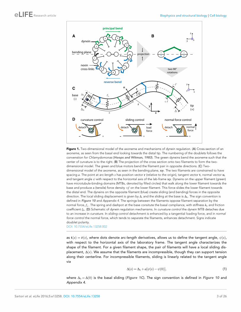