dynamic control of formula - towards driverless
TRANSCRIPT
Dynamic Control of Formula - Towards Driverless
Jing Lu
A thesis
submitted in partial fulfillment of therequirements for the degree of
Master of Science in Mechanical Engineering
University of Washington2020
Committee:Ashley F. EmeryRobert B. Darling
Joseph Garbini
Program Authorized to Offer Degree:Mechanical Engineering
1

c©Copyright 2020Jing Lu
2
Abstract
Dynamic Control of Formula - Towards Driverless
Jing Lu
Chair of the Supervisory Committee:
Ashley F. Emery
Department of Mechanical Engineering
This paper presents vehicle dynamic control algorithms for a dual-motor rear-wheel-drive electric racingcar of UW Formula Motorsports. Team-31 vehicle was designed for human driver only, so the team pro-posed an PID (proportional-integral-derivative) based yaw rate and slip ratio control on dynamic bicycle orfour-wheel vehicle dynamics model. The algorithm aimed to improve acceleration behavior in straight-lineevent and cornering maneuverability. It will also serve as the low-level stability control for the futureautonomous racing car.
Team-32 aimed to compete in FSG driverless events in 2022 - 2023, so the control system should merge intoautonomous driving hardware platform with a MPC (model predictive control) based trajectory trackingalgorithm. Vehicle behavior and control effectiveness were analyzed using MATLAB Simulink, and hope-fully would be validated in HiL (Hardware-in-loop) setup or RC car in the future.
In Section 2: Vehicle handling and performance, the author explained the derivation of vehicle lateral andlongitudinal dynamics model, critical parameters for cornering behavior evaluation and their effects onturn stability. Analysis of a traditional torque vectoring and traction control strategy was explained understeady states condition. In section 3: Model predictive control for autonomous driving, an optimization-based trajectory tracking method was introduced based on kinematic vehicle model. The controller behaviorwas evaluated under simulated competition events. Section 4: Hardware implementation covered key pointsin modeling and configuring critical actuators and sensors for vehicle test preparation.
3
Contents
1 Introduction 6
1.1 Dynamic Control Milestones . . . . . . . . . . . . . . . . . . . . . . . . . . . . . . . . . . . . . . 6
1.2 Autonomous Driving Overview . . . . . . . . . . . . . . . . . . . . . . . . . . . . . . . . . . . . 6
1.3 FSG Motivation . . . . . . . . . . . . . . . . . . . . . . . . . . . . . . . . . . . . . . . . . . . . 7
2 Vehicle Handling Performance 8
2.1 Bicycle Model . . . . . . . . . . . . . . . . . . . . . . . . . . . . . . . . . . . . . . . . . . . . . . 8
2.2 Yaw Stability . . . . . . . . . . . . . . . . . . . . . . . . . . . . . . . . . . . . . . . . . . . . . . 9
2.3 Understeer & Oversteer . . . . . . . . . . . . . . . . . . . . . . . . . . . . . . . . . . . . . . . . 10
2.4 Torque Vectoring & Traction Control . . . . . . . . . . . . . . . . . . . . . . . . . . . . . . . . . 12
2.4.1 Slip Ratio . . . . . . . . . . . . . . . . . . . . . . . . . . . . . . . . . . . . . . . . . . . . 12
2.4.2 Slip Angle . . . . . . . . . . . . . . . . . . . . . . . . . . . . . . . . . . . . . . . . . . . . 13
2.4.3 Tire Force Estimation . . . . . . . . . . . . . . . . . . . . . . . . . . . . . . . . . . . . . 13
2.4.4 Body Force Estimation on Four-Wheels . . . . . . . . . . . . . . . . . . . . . . . . . . . 14
2.4.5 Control Design . . . . . . . . . . . . . . . . . . . . . . . . . . . . . . . . . . . . . . . . . 15
2.4.6 Results . . . . . . . . . . . . . . . . . . . . . . . . . . . . . . . . . . . . . . . . . . . . . 16
3 MPC for Autonomous Driving 20
3.1 Overview . . . . . . . . . . . . . . . . . . . . . . . . . . . . . . . . . . . . . . . . . . . . . . . . 20
3.2 Vehicle Model for MPC . . . . . . . . . . . . . . . . . . . . . . . . . . . . . . . . . . . . . . . . 20
3.3 Prediction & Control . . . . . . . . . . . . . . . . . . . . . . . . . . . . . . . . . . . . . . . . . . 21
4 Hardware Implementation 24
4.1 System Identification . . . . . . . . . . . . . . . . . . . . . . . . . . . . . . . . . . . . . . . . . . 24
4.2 Pedal Map . . . . . . . . . . . . . . . . . . . . . . . . . . . . . . . . . . . . . . . . . . . . . . . . 25
4.3 IMU . . . . . . . . . . . . . . . . . . . . . . . . . . . . . . . . . . . . . . . . . . . . . . . . . . . 26
4.3.1 Error Model . . . . . . . . . . . . . . . . . . . . . . . . . . . . . . . . . . . . . . . . . . . 26
4.3.2 Calibration Method . . . . . . . . . . . . . . . . . . . . . . . . . . . . . . . . . . . . . . 27
5 Conclusion and Outlook 29
6 Acknowledgement 30
4

7 Appendix 31
5
1 Introduction
1.1 Dynamic Control Milestones
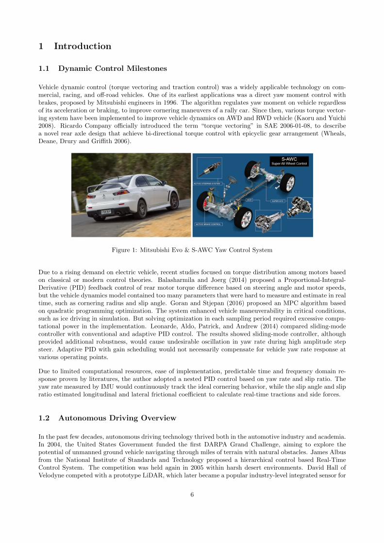
Vehicle dynamic control (torque vectoring and traction control) was a widely applicable technology on com-mercial, racing, and off-road vehicles. One of its earliest applications was a direct yaw moment control withbrakes, proposed by Mitsubishi engineers in 1996. The algorithm regulates yaw moment on vehicle regardlessof its acceleration or braking, to improve cornering maneuvers of a rally car. Since then, various torque vector-ing system have been implemented to improve vehicle dynamics on AWD and RWD vehicle (Kaoru and Yuichi2008). Ricardo Company officially introduced the term “torque vectoring” in SAE 2006-01-08, to describea novel rear axle design that achieve bi-directional torque control with epicyclic gear arrangement (Wheals,Deane, Drury and Griffith 2006).
Figure 1: Mitsubishi Evo & S-AWC Yaw Control System
Due to a rising demand on electric vehicle, recent studies focused on torque distribution among motors basedon classical or modern control theories. Balasharmila and Joerg (2014) proposed a Proportional-Integral-Derivative (PID) feedback control of rear motor torque difference based on steering angle and motor speeds,but the vehicle dynamics model contained too many parameters that were hard to measure and estimate in realtime, such as cornering radius and slip angle. Goran and Stjepan (2016) proposed an MPC algorithm basedon quadratic programming optimization. The system enhanced vehicle maneuverability in critical conditions,such as ice driving in simulation. But solving optimization in each sampling period required excessive compu-tational power in the implementation. Leonarde, Aldo, Patrick, and Andrew (2014) compared sliding-modecontroller with conventional and adaptive PID control. The results showed sliding-mode controller, althoughprovided additional robustness, would cause undesirable oscillation in yaw rate during high amplitude stepsteer. Adaptive PID with gain scheduling would not necessarily compensate for vehicle yaw rate response atvarious operating points.
Due to limited computational resources, ease of implementation, predictable time and frequency domain re-sponse proven by literatures, the author adopted a nested PID control based on yaw rate and slip ratio. Theyaw rate measured by IMU would continuously track the ideal cornering behavior, while the slip angle and slipratio estimated longitudinal and lateral frictional coefficient to calculate real-time tractions and side forces.
1.2 Autonomous Driving Overview
In the past few decades, autonomous driving technology thrived both in the automotive industry and academia.In 2004, the United States Government funded the first DARPA Grand Challenge, aiming to explore thepotential of unmanned ground vehicle navigating through miles of terrain with natural obstacles. James Albusfrom the National Institute of Standards and Technology proposed a hierarchical control based Real-TimeControl System. The competition was held again in 2005 within harsh desert environments. David Hall ofVelodyne competed with a prototype LiDAR, which later became a popular industry-level integrated sensor for
6
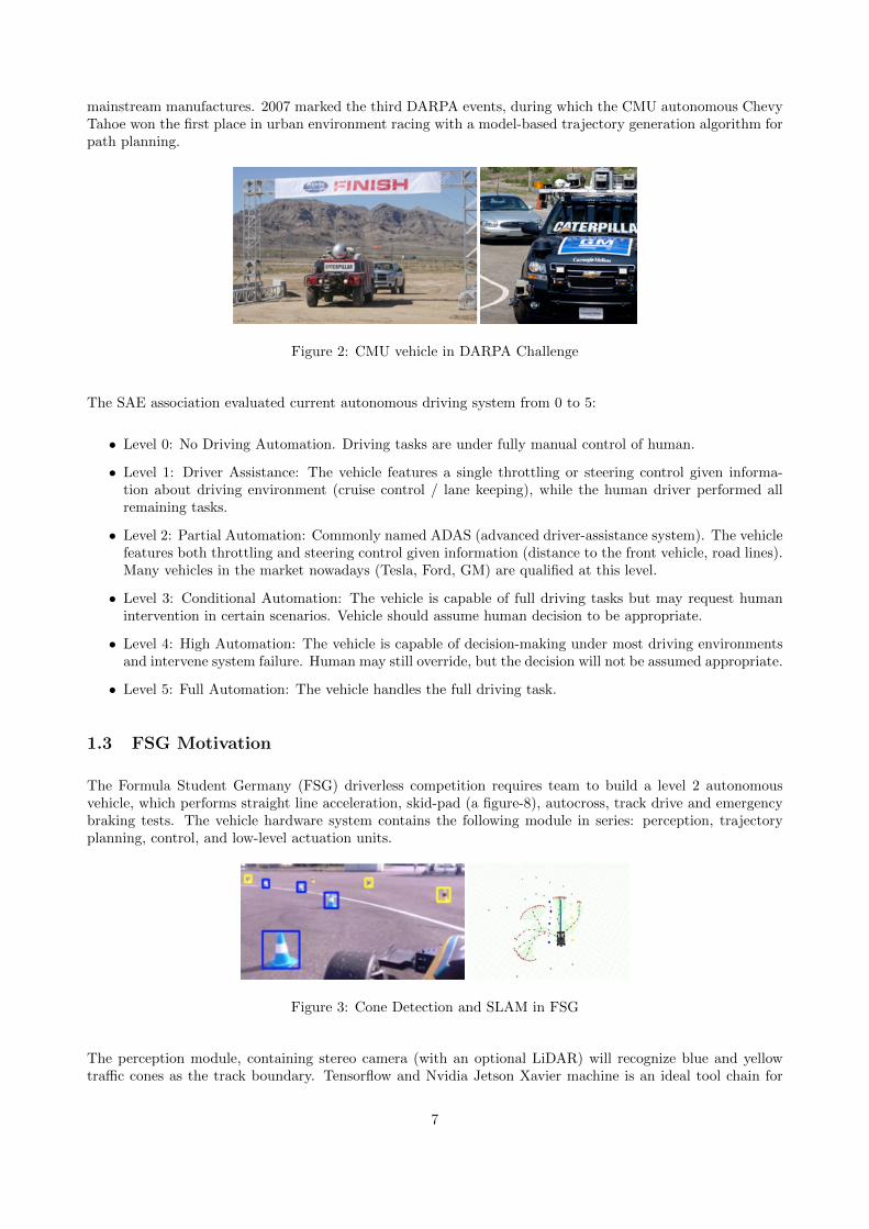
mainstream manufactures. 2007 marked the third DARPA events, during which the CMU autonomous ChevyTahoe won the first place in urban environment racing with a model-based trajectory generation algorithm forpath planning.
Figure 2: CMU vehicle in DARPA Challenge
The SAE association evaluated current autonomous driving system from 0 to 5:
• Level 0: No Driving Automation. Driving tasks are under fully manual control of human.
• Level 1: Driver Assistance: The vehicle features a single throttling or steering control given informa-tion about driving environment (cruise control / lane keeping), while the human driver performed allremaining tasks.
• Level 2: Partial Automation: Commonly named ADAS (advanced driver-assistance system). The vehiclefeatures both throttling and steering control given information (distance to the front vehicle, road lines).Many vehicles in the market nowadays (Tesla, Ford, GM) are qualified at this level.
• Level 3: Conditional Automation: The vehicle is capable of full driving tasks but may request humanintervention in certain scenarios. Vehicle should assume human decision to be appropriate.
• Level 4: High Automation: The vehicle is capable of decision-making under most driving environmentsand intervene system failure. Human may still override, but the decision will not be assumed appropriate.
• Level 5: Full Automation: The vehicle handles the full driving task.
1.3 FSG Motivation
The Formula Student Germany (FSG) driverless competition requires team to build a level 2 autonomousvehicle, which performs straight line acceleration, skid-pad (a figure-8), autocross, track drive and emergencybraking tests. The vehicle hardware system contains the following module in series: perception, trajectoryplanning, control, and low-level actuation units.
Figure 3: Cone Detection and SLAM in FSG
The perception module, containing stereo camera (with an optional LiDAR) will recognize blue and yellowtraffic cones as the track boundary. Tensorflow and Nvidia Jetson Xavier machine is an ideal tool chain for
7
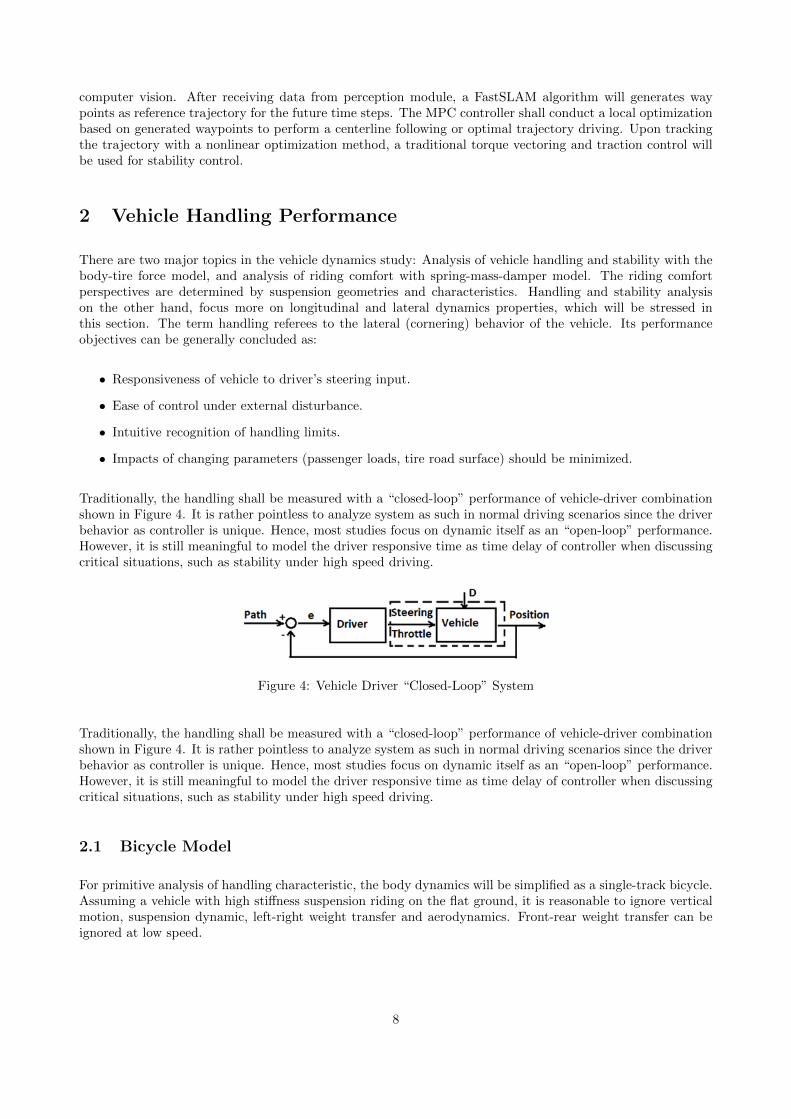
computer vision. After receiving data from perception module, a FastSLAM algorithm will generates waypoints as reference trajectory for the future time steps. The MPC controller shall conduct a local optimizationbased on generated waypoints to perform a centerline following or optimal trajectory driving. Upon trackingthe trajectory with a nonlinear optimization method, a traditional torque vectoring and traction control willbe used for stability control.
2 Vehicle Handling Performance
There are two major topics in the vehicle dynamics study: Analysis of vehicle handling and stability with thebody-tire force model, and analysis of riding comfort with spring-mass-damper model. The riding comfortperspectives are determined by suspension geometries and characteristics. Handling and stability analysison the other hand, focus more on longitudinal and lateral dynamics properties, which will be stressed inthis section. The term handling referees to the lateral (cornering) behavior of the vehicle. Its performanceobjectives can be generally concluded as:
• Responsiveness of vehicle to driver’s steering input.
• Ease of control under external disturbance.
• Intuitive recognition of handling limits.
• Impacts of changing parameters (passenger loads, tire road surface) should be minimized.
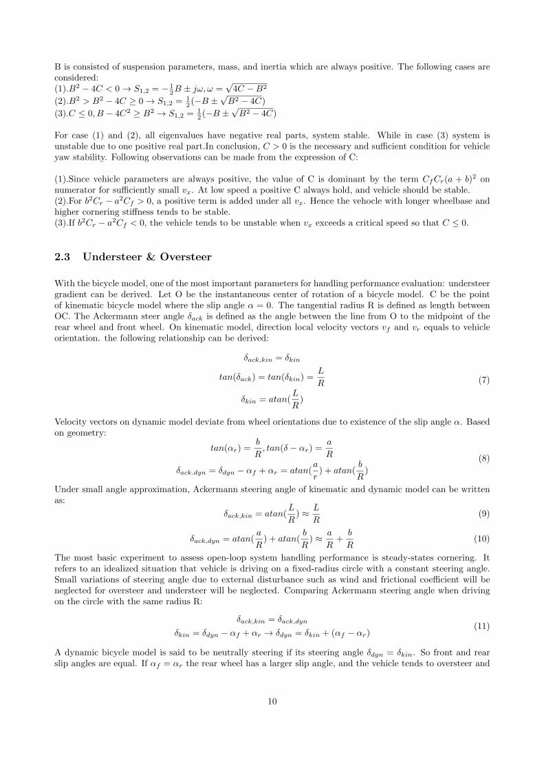
Traditionally, the handling shall be measured with a “closed-loop” performance of vehicle-driver combinationshown in Figure 4. It is rather pointless to analyze system as such in normal driving scenarios since the driverbehavior as controller is unique. Hence, most studies focus on dynamic itself as an “open-loop” performance.However, it is still meaningful to model the driver responsive time as time delay of controller when discussingcritical situations, such as stability under high speed driving.
Figure 4: Vehicle Driver “Closed-Loop” System
Traditionally, the handling shall be measured with a “closed-loop” performance of vehicle-driver combinationshown in Figure 4. It is rather pointless to analyze system as such in normal driving scenarios since the driverbehavior as controller is unique. Hence, most studies focus on dynamic itself as an “open-loop” performance.However, it is still meaningful to model the driver responsive time as time delay of controller when discussingcritical situations, such as stability under high speed driving.
2.1 Bicycle Model
For primitive analysis of handling characteristic, the body dynamics will be simplified as a single-track bicycle.Assuming a vehicle with high stiffness suspension riding on the flat ground, it is reasonable to ignore verticalmotion, suspension dynamic, left-right weight transfer and aerodynamics. Front-rear weight transfer can beignored at low speed.
8
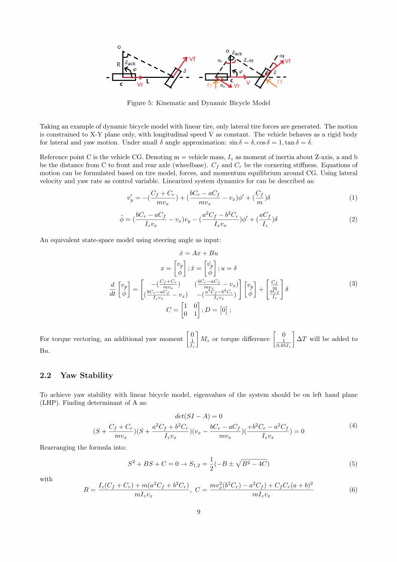
Figure 5: Kinematic and Dynamic Bicycle Model
Taking an example of dynamic bicycle model with linear tire, only lateral tire forces are generated. The motionis constrained to X-Y plane only, with longitudinal speed V as constant. The vehicle behaves as a rigid bodyfor lateral and yaw motion. Under small δ angle approximation: sin δ = δ, cos δ = 1, tan δ = δ.
Reference point C is the vehicle CG. Denoting m = vehicle mass, Iz as moment of inertia about Z-axis, a and bbe the distance from C to front and rear axle (wheelbase). Cf and Cr be the cornering stiffness. Equations ofmotion can be formulated based on tire model, forces, and momentum equilibrium around CG. Using lateralvelocity and yaw rate as control variable. Linearized system dynamics for can be described as:
v′y = −(Cf + Crmvx
) + (bCr − aCf
mvx− vx)φ′ + (
Cfm
)δ (1)
φ = (bCr − aCf
Izvx− vx)vy − (
a2Cf − b2CrIxvx
)φ′ + (aCfIz
)δ (2)
An equivalent state-space model using steering angle as input:
x = Ax+Bu
x =
[vyφ
]; x =
[vyφ
];u = δ
d
dt
[vyφ
]=
[−(
Cf+Cr
mvx) (
bCr−aCf
mvx− vx)
(bCr−aCf
Izvx− vx) −(
a2Cf−b2Cr
Izvx)
] [vyφ
]+
[Cf
maCf
Iz
]δ
C =
[1 00 1
];D =
[0]
;
(3)
For torque vectoring, an additional yaw moment
[01Iz
]Mz or torque difference
[01
0.05Iz
]∆T will be added to
Bu.
2.2 Yaw Stability
To achieve yaw stability with linear bicycle model, eigenvalues of the system should be on left hand plane(LHP). Finding determinant of A as:
det(SI −A) = 0
(S +Cf + Crmvx
)(S +a2Cf + b2Cr
Izvx)(vx −
bCr − aCfmvx
)(+b2Cr − a2Cf
Izvx) = 0
(4)
Rearranging the formula into:
S2 +BS + C = 0→ S1,2 =1
2(−B ±
√B2 − 4C) (5)
with
B =Iz(Cf + Cr) +m(a2Cf + b2Cr)
mIzvx, C =
mv2x(b2Cr)− a2Cf ) + CfCr(a+ b)2
mIzvx(6)
9
B is consisted of suspension parameters, mass, and inertia which are always positive. The following cases areconsidered:(1).B2 − 4C < 0→ S1,2 = − 1
2B ± jω, ω =√
4C −B2
(2).B2 > B2 − 4C ≥ 0→ S1,2 = 12 (−B ±
√B2 − 4C)
(3).C ≤ 0, B − 4C2 ≥ B2 → S1,2 = 12 (−B ±
√B2 − 4C)
For case (1) and (2), all eigenvalues have negative real parts, system stable. While in case (3) system isunstable due to one positive real part.In conclusion, C > 0 is the necessary and sufficient condition for vehicleyaw stability. Following observations can be made from the expression of C:
(1).Since vehicle parameters are always positive, the value of C is dominant by the term CfCr(a + b)2 onnumerator for sufficiently small vx. At low speed a positive C always hold, and vehicle should be stable.(2).For b2Cr − a2Cf > 0, a positive term is added under all vx. Hence the vehocle with longer wheelbase andhigher cornering stiffness tends to be stable.(3).If b2Cr − a2Cf < 0, the vehicle tends to be unstable when vx exceeds a critical speed so that C ≤ 0.
2.3 Understeer & Oversteer
With the bicycle model, one of the most important parameters for handling performance evaluation: understeergradient can be derived. Let O be the instantaneous center of rotation of a bicycle model. C be the pointof kinematic bicycle model where the slip angle α = 0. The tangential radius R is defined as length betweenOC. The Ackermann steer angle δack is defined as the angle between the line from O to the midpoint of therear wheel and front wheel. On kinematic model, direction local velocity vectors vf and vr equals to vehicleorientation. the following relationship can be derived:
δack,kin = δkin
tan(δack) = tan(δkin) =L
R
δkin = atan(L
R)
(7)
Velocity vectors on dynamic model deviate from wheel orientations due to existence of the slip angle α. Basedon geometry:
tan(αr) =b
R, tan(δ − αr) =
a
R
δack.dyn = δdyn − αf + αr = atan(a
r) + atan(
b
R)
(8)
Under small angle approximation, Ackermann steering angle of kinematic and dynamic model can be writtenas:
δack,kin = atan(L
R) ≈ L
R(9)
δack,dyn = atan(a
R) + atan(
b
R) ≈ a
R+b
R(10)
The most basic experiment to assess open-loop system handling performance is steady-states cornering. Itrefers to an idealized situation that vehicle is driving on a fixed-radius circle with a constant steering angle.Small variations of steering angle due to external disturbance such as wind and frictional coefficient will beneglected for oversteer and understeer will be neglected. Comparing Ackermann steering angle when drivingon the circle with the same radius R:
δack,kin = δack,dyn
δkin = δdyn − αf + αr → δdyn = δkin + (αf − αr)(11)
A dynamic bicycle model is said to be neutrally steering if its steering angle δdyn = δkin. So front and rearslip angles are equal. If αf = αr the rear wheel has a larger slip angle, and the vehicle tends to oversteer and
10
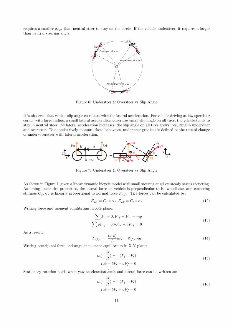
requires a smaller δdyn than neutral steer to stay on the circle. If the vehicle understeer, it requires a largerthan neutral steering angle.
Figure 6: Understeer & Oversteer vs Slip Angle
It is observed that vehicle slip angle co-relates with the lateral acceleration. For vehicle driving at low speeds orcorner with large radius, a small lateral acceleration generates small slip angle on all tires, the vehicle tends tostay in neutral steer. As lateral acceleration increases, the slip angle on all tires grows, resulting in understeerand oversteer. To quantitatively measure these behaviors, understeer gradient is defined as the rate of changeof under/oversteer with lateral acceleration.
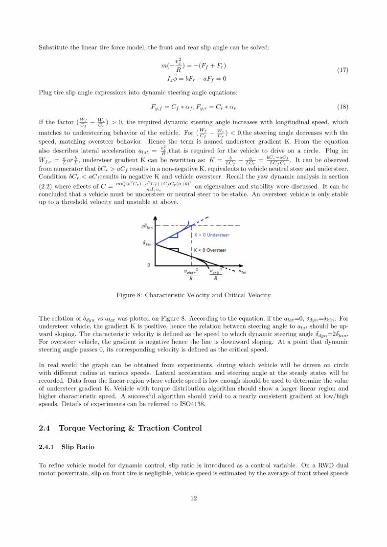
Figure 7: Understeer & Oversteer vs Slip Angle
As shown in Figure 7, given a linear dynamic bicycle model with small steering angel on steady states cornering.Assuming linear tire properties, the lateral force on vehicle is perpendicular to its wheelbase, and corneringstiffness Cf , Cr is linearly proportional to normal force Fz,fr. Tire forces can be calculated by:
Fy,f = Cf ∗ αf , Fy,r = Cr ∗ αr (12)
Writing force and moment equilibrium in X-Z plane:∑Fz = 0, Fzf + Fzr = mg∑
Mi,y = 0, bFzr − aFzf = 0(13)
As a result:
Fzf,zr =(a, b)
Lmg = Wf,rmg (14)
Writing centripetal force and angular moment equilibrium in X-Y plane:
m(−v2x
R) = −(Ff + Fr)
Izφ = bFr − aFf = 0
(15)
Stationary rotation holds when yaw acceleration φ=0, and lateral force can be written as:
m(−v2x
R) = −(Ff + Fr)
Izφ = bFr − aFf = 0
(16)
11
Substitute the linear tire force model, the front and rear slip angle can be solved:
m(−v2x
R) = −(Ff + Fr)
Izφ = bFr − aFf = 0
(17)
Plug tire slip angle expressions into dynamic steering angle equations:
Fy,f = Cf ∗ αf , Fy,r = Cr ∗ αr (18)
If the factor (Wf
Cf− Wr
Cr) > 0, the required dynamic steering angle increases with longitudinal speed, which
matches to understeering behavior of the vehicle. For (Wf
Cf− Wr
Cr) < 0,the steering angle decreases with the
speed, matching oversteer behavior. Hence the term is named understeer gradient K. From the equation
also describes lateral acceleration alat =v2xR ,that is required for the vehicle to drive on a circle. Plug in:
Wf,r = aLor
bL , understeer gradient K can be rewritten as: K = b
LCf− a
LCr=
bCr−aCf
LCfCr. It can be observed
from numerator that bCr > aCf results in a non-negative K, equivalents to vehicle neutral steer and understeer.Condition bCr < aCf results in negative K and vehicle oversteer. Recall the yaw dynamic analysis in section
(2.2) where effects of C =mv2x(b
2Cr)−a2Cf )+CfCr(a+b)2
mIzvxon eigenvalues and stability were discussed. It can be
concluded that a vehicle must be understeer or neutral steer to be stable. An oversteer vehicle is only stableup to a threshold velocity and unstable at above.
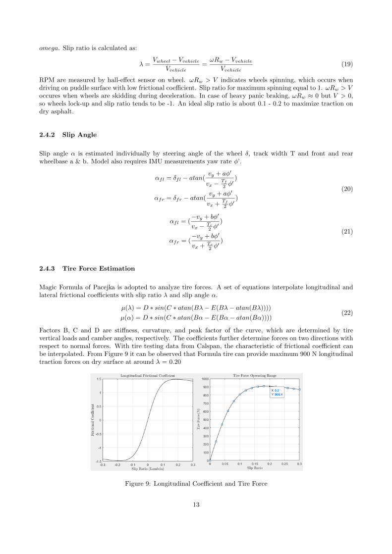
Figure 8: Characteristic Velocity and Critical Velocity
The relation of δdyn vs alat was plotted on Figure 8. According to the equation, if the alat=0, δdyn=δkin. Forundersteer vehicle, the gradient K is positive, hence the relation between steering angle to alat should be up-ward sloping. The characteristic velocity is defined as the speed to which dynamic steering angle δdyn=2δkin.For oversteer vehicle, the gradient is negative hence the line is downward sloping. At a point that dynamicsteering angle passes 0, its corresponding velocity is defined as the critical speed.
In real world the graph can be obtained from experiments, during which vehicle will be driven on circlewith different radius at various speeds. Lateral acceleration and steering angle at the steady states will berecorded. Data from the linear region where vehicle speed is low enough should be used to determine the valueof understeer gradient K. Vehicle with torque distribution algorithm should show a larger linear region andhigher characteristic speed. A successful algorithm should yield to a nearly consistent gradient at low/highspeeds. Details of experiments can be referred to ISO4138.
2.4 Torque Vectoring & Traction Control
2.4.1 Slip Ratio
To refine vehicle model for dynamic control, slip ratio is introduced as a control variable. On a RWD dualmotor powertrain, slip on front tire is negligible, vehicle speed is estimated by the average of front wheel speeds
12
omega. Slip ratio is calculated as:
λ =Vwheel − Vvehicle
Vvehicle=ωRw − Vvehicle
Vvehicle(19)
RPM are measured by hall-effect sensor on wheel. ωRw > V indicates wheels spinning, which occurs whendriving on puddle surface with low frictional coefficient. Slip ratio for maximum spinning equal to 1. ωRw > Voccures when wheels are skidding during deceleration. In case of heavy panic braking, ωRw ≈ 0 but V > 0,so wheels lock-up and slip ratio tends to be -1. An ideal slip ratio is about 0.1 - 0.2 to maximize traction ondry asphalt.
2.4.2 Slip Angle
Slip angle α is estimated individually by steering angle of the wheel δ, track width T and front and rearwheelbase a & b. Model also requires IMU measurements yaw rate φ’.
αfl = δfl − atan(vy + aφ′
vx − Tf
2 φ′)
αfr = δfr − atan(vy + aφ′
vx +Tf
2 φ′)
(20)
αfl = (−vy + bφ′
vx − Tr
2 φ′)
αfr = (−vy + bφ′
vx + Tr
2 φ′)
(21)
2.4.3 Tire Force Estimation
Magic Formula of Pacejka is adopted to analyze tire forces. A set of equations interpolate longitudinal andlateral frictional coefficients with slip ratio λ and slip angle α.
µ(λ) = D ∗ sin(C ∗ atan(Bλ− E(Bλ− atan(Bλ))))
µ(α) = D ∗ sin(C ∗ atan(Bα− E(Bα− atan(Bα))))(22)
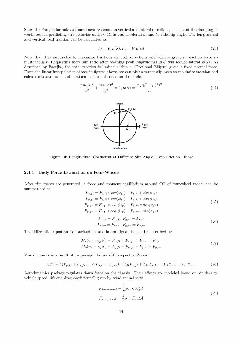
Factors B, C and D are stiffness, curvature, and peak factor of the curve, which are determined by tirevertical loads and camber angles, respectively. The coefficients further determine forces on two directions withrespect to normal forces. With tire testing data from Calspan, the characteristic of frictional coefficient canbe interpolated. From Figure 9 it can be observed that Formula tire can provide maximum 900 N longitudinaltraction forces on dry surface at around λ = 0.20
Figure 9: Longitudinal Coefficient and Tire Force
13
Since the Pacejka formula assumes linear response on vertical and lateral directions, a constant tire damping, itworks best in predicting tire behavior under 0.4G lateral acceleration and 5o side slip angle. The longitudinaland vertical load traction can be calculated as:
Ft = Fzµ(λ), Fs = Fzµ(α) (23)
Note that it is impossible to maximize tractions on both directions and achieve greatest reaction force si-multaneously. Requesting more slip ratio after reaching peak longitudinal µ(λ) will reduce lateral µ(α). Asdescribed by Pacejka, the total traction is limited within a “Frictional Ellipse” given a fixed normal force.From the linear interpolation shown in figures above, we can pick a target slip ratio to maximize traction andcalculate lateral force and frictional coefficient based on the circle.
mu(λ)2
x2+mu(α)2
y2= 1, µ(α) =
x√y2 − µ(λ)2
n(24)
Figure 10: Longitudinal Coefficient at Different Slip Angle Given Friction Ellipse
2.4.4 Body Force Estimation on Four-Wheels
After tire forces are generated, a force and moment equilibrium around CG of four-wheel model can besummarized as:
Fx,fl = Ft,fl ∗ cos(φfl)− Fs,fl ∗ sin(φfl)
Fy,fl = Ft,fl ∗ cos(φfl) + Fs,fl ∗ sin(φfl)
Fx,fr = Ft,fl ∗ cos(φfr)− Fs,fr ∗ sin(φfr)
Fy,fr = Ft,fl ∗ cos(φfr) + Fs,fr ∗ sin(φfr)
(25)
Fx,rl = Ft,rl, Fy,rl = Fs,rl
Fx,rr = Ft,rr, Fy,rr = Fs,rr(26)
The differential equation for longitudinal and lateral dynamics can be described as:
Mv(vx − vyφ′) = Fx,fl + Fx,fr + Fx,rl + Fx,rr
Mv(vx + vyφ′) = Fy,fl + Fy,fr + Fy,rl + Fy,rr
(27)
Yaw dynamics is a result of torque equilibrium with respect to Z-axis:
Izφ′′ = a(Fy,fl + Fy,fr)− b(Fy,rl + Fy,rr)− TflFx,fl + TfrFx,fr − TrlFx,rl + TrrFx,rr (28)
Aerodynamics package regulates down force on the chassis. Their effects are modeled based on air density,vehicle speed, lift and drag coefficient C given by wind tunnel test:
Fdown,total =1
2ρairClv
2xA
Fdrag,total =1
2ρairCdv
2xA
(29)
14
2.4.5 Control Design
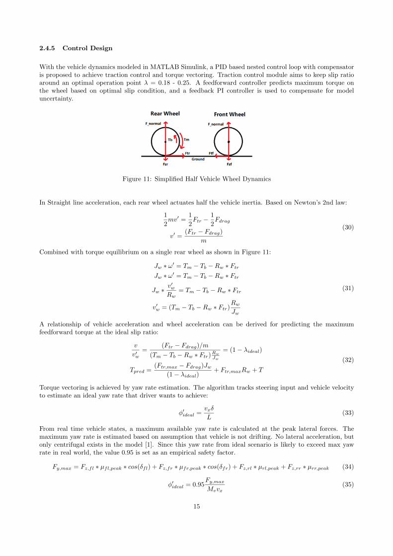
With the vehicle dynamics modeled in MATLAB Simulink, a PID based nested control loop with compensatoris proposed to achieve traction control and torque vectoring. Traction control module aims to keep slip ratioaround an optimal operation point λ = 0.18 - 0.25. A feedforward controller predicts maximum torque onthe wheel based on optimal slip condition, and a feedback PI controller is used to compensate for modeluncertainty.
Figure 11: Simplified Half Vehicle Wheel Dynamics
In Straight line acceleration, each rear wheel actuates half the vehicle inertia. Based on Newton’s 2nd law:
1
2mv′ =
1
2Ftr −
1
2Fdrag
v′ =(Ftr − Fdrag)
m
(30)
Combined with torque equilibrium on a single rear wheel as shown in Figure 11:
Jw ∗ ω′ = Tm − Tb −Rw ∗ FtrJw ∗ ω′ = Tm − Tb −Rw ∗ Ftr
Jw ∗v′wRw
= Tm − Tb −Rw ∗ Ftr
v′w = (Tm − Tb −Rw ∗ Ftr)RwJw
(31)
A relationship of vehicle acceleration and wheel acceleration can be derived for predicting the maximumfeedforward torque at the ideal slip ratio:
v
v′w=
(Ftr − Fdrag)/m(Tm − Tb −Rw ∗ Ftr)Rw
Jw
= (1− λideal)
Tpred =(Ftr,max − Fdrag)Jw
(1− λideal)+ Ftr,maxRw + T
(32)
Torque vectoring is achieved by yaw rate estimation. The algorithm tracks steering input and vehicle velocityto estimate an ideal yaw rate that driver wants to achieve:
φ′ideal =vxδ
L(33)
From real time vehicle states, a maximum available yaw rate is calculated at the peak lateral forces. Themaximum yaw rate is estimated based on assumption that vehicle is not drifting. No lateral acceleration, butonly centrifugal exists in the model [1]. Since this yaw rate from ideal scenario is likely to exceed max yawrate in real world, the value 0.95 is set as an empirical safety factor.
Fy,max = Fz,fl ∗ µfl,peak ∗ cos(δfl) + Fz,fr ∗ µfr,peak ∗ cos(δfr) + Fz,rl ∗ µrl,peak + Fz,rr ∗ µrr,peak (34)
φ′ideal = 0.95Fy,maxMvvx
(35)
15
For skidpad events, the vehicle drives two laps on a “figure-8” with constant radius. Vehicle reaches steadystates in middle of the 1st lap and maintain such dynamics until cornering exit. The max yaw rate in this casemaintains constant as:
φ′skid =vxR
(36)
It is reasonable to set φ′skid as control target during skidpad event. Once optimal yaw rate is not dependingon steering angle, driver may adjust steering angle to achieve a time-saving trajectory: by slightly decreasingsteering angle, a larger traction force will be distributed to longitudinal direction, so vehicle speed will increase[1]. During track drive, system sets φ′ideal as the control target to achieve driver intended maneuvers unlessφ′ideal > φ′max. A proportional controller distributes torque difference between two rear wheels:
∆T = Kp(φ′target − φ′measured) (37)
Oversteer sometimes occurs when driver requests yaw rate drastically at performance limits. Most tractionsare distributed on longitudinal direction to achieve high speed. And vehicle tends to slide out due to lack oflateral tractions that maintain angular motion. To fix this, driver commonly releases throttle and applies anopposite steer. In order not to intervene driver’s instinct, system compares direction of φ′measured and φ′idealto detect counter-steer action, and assists vehicle status recovering by applying torque as below:
∆Tcountersteer = ∆T (1− |φ′ideal|φ′limit
), φ′limit = 0.25 (rad/s) (38)
When torque requests from traction control and torque vectoring modules are infused, a logic check is set priorto inverter and motor, such that:
∆T = TR − TLmax(TR, TL) = min(Trequest − TTCmax(R,L))
(39)
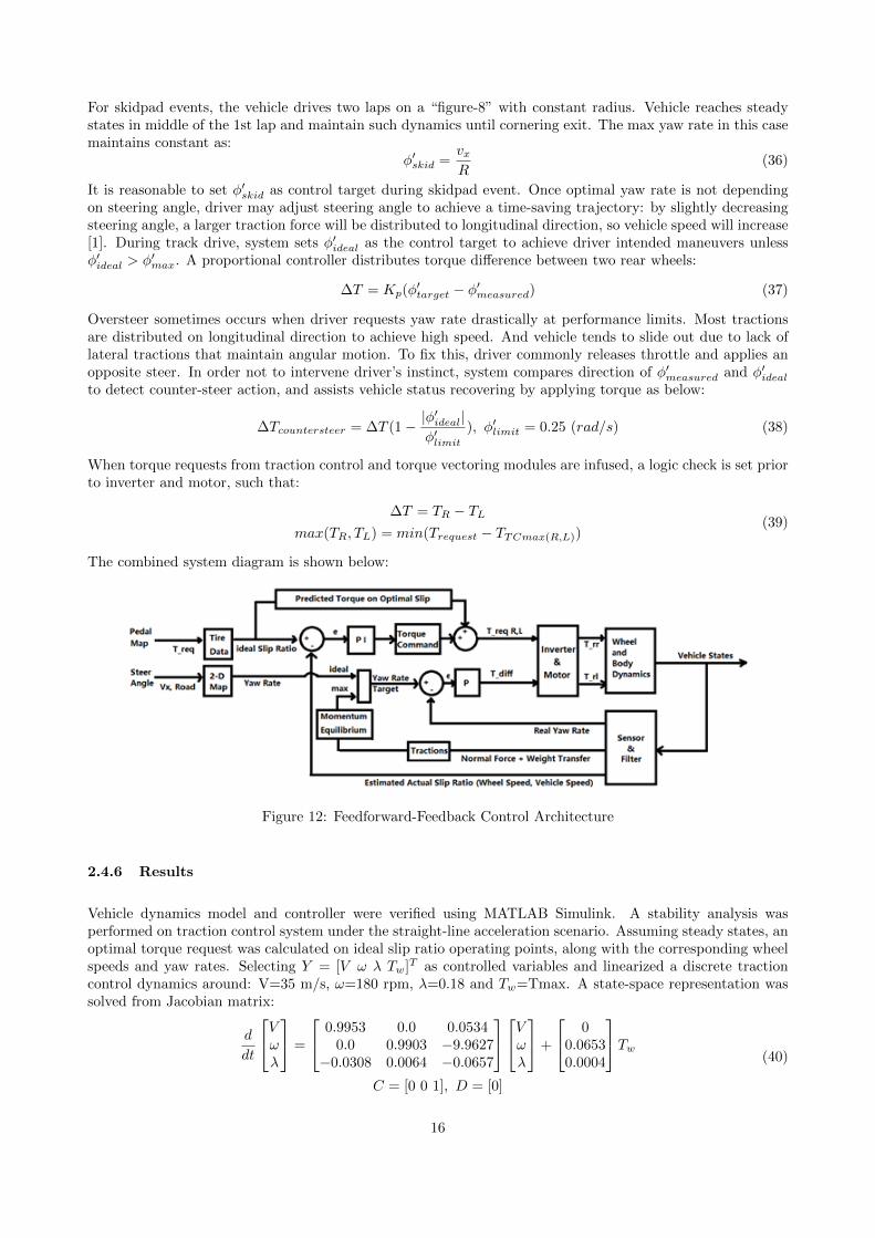
The combined system diagram is shown below:
Figure 12: Feedforward-Feedback Control Architecture
2.4.6 Results
Vehicle dynamics model and controller were verified using MATLAB Simulink. A stability analysis wasperformed on traction control system under the straight-line acceleration scenario. Assuming steady states, anoptimal torque request was calculated on ideal slip ratio operating points, along with the corresponding wheelspeeds and yaw rates. Selecting Y = [V ω λ Tw]T as controlled variables and linearized a discrete tractioncontrol dynamics around: V=35 m/s, ω=180 rpm, λ=0.18 and Tw=Tmax. A state-space representation wassolved from Jacobian matrix:
d
dt
Vωλ
=
0.9953 0.0 0.05340.0 0.9903 −9.9627
−0.0308 0.0064 −0.0657
Vωλ
+
00.06530.0004
TwC = [0 0 1], D = [0]
(40)
16
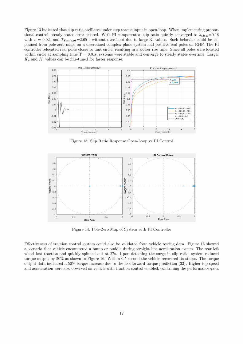
Figure 13 indicated that slip ratio oscillates under step torque input in open-loop. When implementing propor-tional control, steady states error existed. With PI compensator, slip ratio quickly converged to λideal=0.18with τ = 0.02s and TSettle,98=2.65 s without overshoot due to large Ki values. Such behavior could be ex-plained from pole-zero map: on a discretized complex plane system had positive real poles on RHP. The PIcontroller relocated real poles closer to unit circle, resulting in a slower rise time. Since all poles were locatedwithin circle at sampling time T = 0.01s, systems were stable and converge to steady states overtime. LargerKp and Ki values can be fine-tuned for faster response.
Figure 13: Slip Ratio Response Open-Loop vs PI Control
Figure 14: Pole-Zero Map of System with PI Controller
Effectiveness of traction control system could also be validated from vehicle testing data. Figure 15 showeda scenario that vehicle encountered a bump or puddle during straight line acceleration events. The rear leftwheel lost traction and quickly spinned out at 27s. Upon detecting the surge in slip ratio, system reducedtorque output by 50% as shown in Figure 16. Within 0.5 second the vehicle recovered its status. The torqueoutput data indicated a 50% torque increase due to the feedforward torque prediction (32). Higher top speedand acceleration were also observed on vehicle with traction control enabled, confirming the performance gain.
17
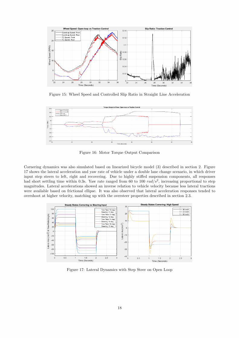
Figure 15: Wheel Speed and Controlled Slip Ratio in Straight Line Acceleration
Figure 16: Motor Torque Output Comparison
Cornering dynamics was also simulated based on linearized bicycle model (3) described in section 2. Figure17 shows the lateral acceleration and yaw rate of vehicle under a double lane change scenario, in which driverinput step steers to left, right and recovering. Due to highly stiffed suspension components, all responseshad short settling time within 0.3s. Yaw rate ranged from 60 to 100 rad/s2, increasing proportional to stepmagnitudes. Lateral accelerations showed an inverse relation to vehicle velocity because less lateral tractionswere available based on frictional ellipse. It was also observed that lateral acceleration responses tended toovershoot at higher velocity, matching up with the oversteer properties described in section 2.3.
Figure 17: Lateral Dynamics with Step Steer on Open Loop
18
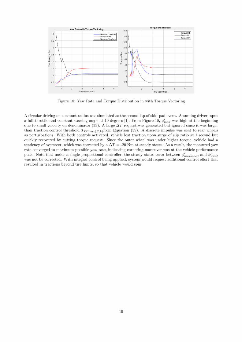
Figure 18: Yaw Rate and Torque Distribution in with Torque Vectoring
A circular driving on constant radius was simulated as the second lap of skid-pad event. Assuming driver inputa full throttle and constant steering angle at 10 degrees [1]. From Figure 18, φ′max was high at the beginningdue to small velocity on denominator (33). A large ∆T request was generated but ignored since it was largerthan traction control threshold TTCmax(R,L)from Equation (39). A discrete impulse was sent to rear wheelsas perturbations. With both controls activated, vehicle lost traction upon surge of slip ratio at 1 second butquickly recovered by cutting torque request. Since the outer wheel was under higher torque, vehicle had atendency of oversteer, which was corrected by a ∆T = -20 Nm at steady states. As a result, the measured yawrate converged to maximum possible yaw rate, indicating cornering maneuver was at the vehicle performancepeak. Note that under a single proportional controller, the steady states error between φ′measured and φ′idealwas not be corrected. With integral control being applied, system would request additional control effort thatresulted in tractions beyond tire limits, so that vehicle would spin.
19
3 MPC for Autonomous Driving
3.1 Overview
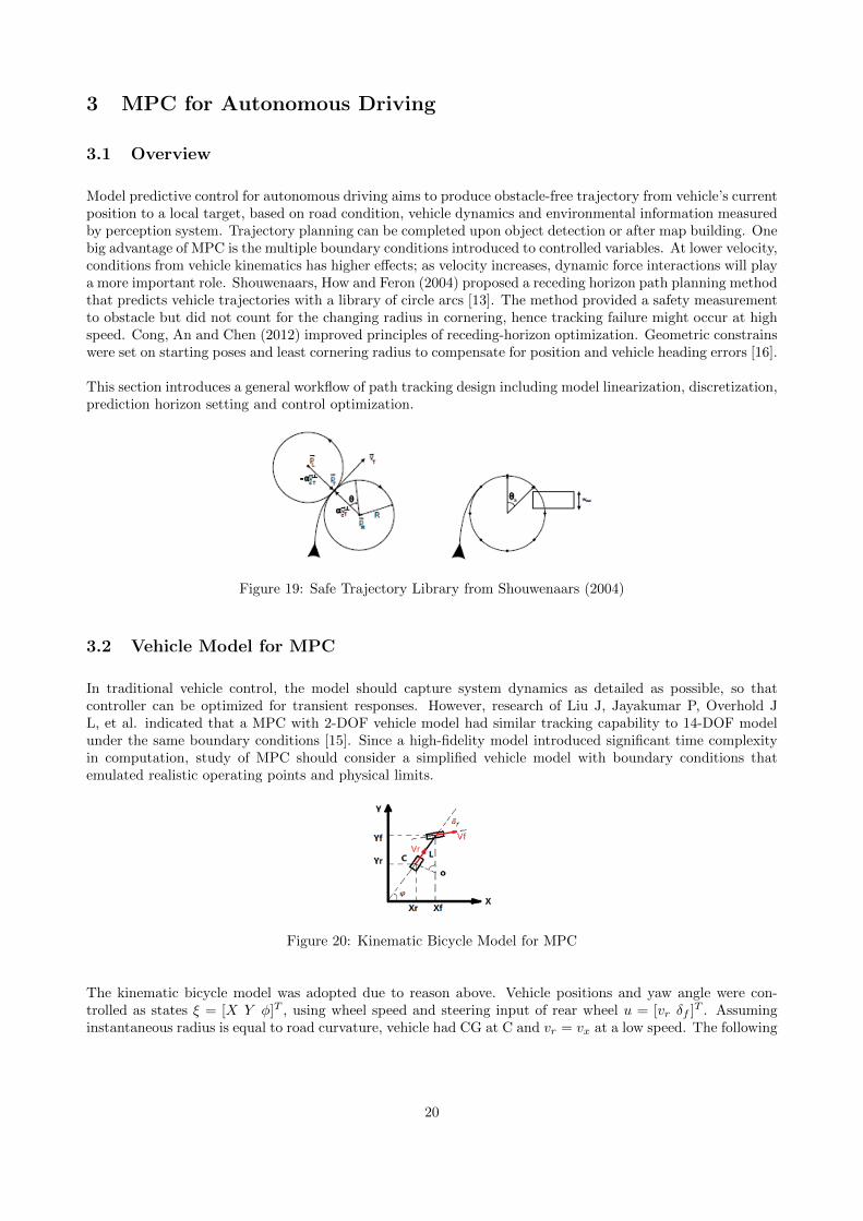
Model predictive control for autonomous driving aims to produce obstacle-free trajectory from vehicle’s currentposition to a local target, based on road condition, vehicle dynamics and environmental information measuredby perception system. Trajectory planning can be completed upon object detection or after map building. Onebig advantage of MPC is the multiple boundary conditions introduced to controlled variables. At lower velocity,conditions from vehicle kinematics has higher effects; as velocity increases, dynamic force interactions will playa more important role. Shouwenaars, How and Feron (2004) proposed a receding horizon path planning methodthat predicts vehicle trajectories with a library of circle arcs [13]. The method provided a safety measurementto obstacle but did not count for the changing radius in cornering, hence tracking failure might occur at highspeed. Cong, An and Chen (2012) improved principles of receding-horizon optimization. Geometric constrainswere set on starting poses and least cornering radius to compensate for position and vehicle heading errors [16].
This section introduces a general workflow of path tracking design including model linearization, discretization,prediction horizon setting and control optimization.
Figure 19: Safe Trajectory Library from Shouwenaars (2004)
3.2 Vehicle Model for MPC
In traditional vehicle control, the model should capture system dynamics as detailed as possible, so thatcontroller can be optimized for transient responses. However, research of Liu J, Jayakumar P, Overhold JL, et al. indicated that a MPC with 2-DOF vehicle model had similar tracking capability to 14-DOF modelunder the same boundary conditions [15]. Since a high-fidelity model introduced significant time complexityin computation, study of MPC should consider a simplified vehicle model with boundary conditions thatemulated realistic operating points and physical limits.
Figure 20: Kinematic Bicycle Model for MPC
The kinematic bicycle model was adopted due to reason above. Vehicle positions and yaw angle were con-trolled as states ξ = [X Y φ]T , using wheel speed and steering input of rear wheel u = [vr δf ]T . Assuminginstantaneous radius is equal to road curvature, vehicle had CG at C and vr = vx at a low speed. The following
20
equation of motions were written:vfcos(δf ) = vr, vfsin(δf ) = vy
vy = vrtan(δf ), φ′ = vftan(δf )
L
(41)
A nonlinear state space was derived:
d
dy
XYφ
=
cos(φ)sin(φ)
0
vr +
001
φ′ =
cos(φ)sin(φ)tan(δf )
L
(42)
Apply linear approximation. Assuming a reference system passed waypoints on ideal trajectory so that statesand control input of reference system at any time can be measured:
ξ′ref = f(ξref , uref ) (43)
Errors between measured system and referenced system can be derived as:
ξe = ξ − ξr =
X −Xr
Y − Yrφ− φr
, ue = u− ur =
[vr − vrefδf − δref
](44)
Solving a 1st order Tayler Series expansion at reference trajectory (ξref , uref ):
ξ′ = f(ξref , uref ) +df
dξ(ξ − ξr) +
df
du(u− ur) (45)
Subtracted equation (43) from equation (45), the state space of vehicle error states was derived:
ξe = ξ − ξr =df
dξ(ξ − ξ(r)) +
df
du(u− ur) (46)
ξ′e = Aξe +Bue (47)
Where A,B should be solved as Jacobian matrix Jf (x1 . . . xn) =
dy1dx1
. . . dy1dyn
.... . .
...dymdx1
. . . dymdyn
, as a result:
d
dy
Xe
Yeφe
=
0 0 −vrsin(φr)0 0 vrcos(φr)0 0 0
cos(φr) 0sin(φr) 0tan(δf )
Lvr
Lcos2(δf )
[vr,eδf,e
](48)
The state space was further discretized with Forward-Euler method, where A=(I+TA),B=(TB). Given:
ξe =ξe(k + 1)− ξe(k)
T= Aξe(k) +Bue(k)
ξe(k + 1) = A(k)ξe(k) +B(k)ue(k) = (I + TA)ξe(k) + (TB)ue(k)(49)
As a result, a linear time variant states-space for vehicle state-error dynamics was derived:
d
dy
Xe
Yeφe
=
1 0 −Tvrsin(φr)0 1 Tvrcos(φr)0 0 1
Tcos(φr) 0Tsin(φr) 0
Ttan(δf )
L T vrLcos2(δf )
[vr,eδf,e
](50)
3.3 Prediction & Control
Based on equation (49), setting prediction horizon Np = 4 and control horizon Nc = 3, the effect of controleffort ue(k) to vehicle states and outputs within horizon should be:
21

ξe(k + 1) = Aξe(k) +Bue(k)ξe(k + 2) = A2ξe(k) +ABue(k) +Bue(k + 1)ξe(k + 3) = A3ξe(k) +A2Bue(k) +ABue(k + 1) +Bue(k + 2)ξe(k + 4) = A4ξe(k) +A3Bue(k) +A2Bue(k + 1) +ABue(k + 2) +Bue(k + 3)Equations could be summarized as a general form:
Y = Aξe(k) + BU(k)
Y =
ξe(k + 1)...
ξe(k +Np)
A =
A...ANp
ξe(k) =
Xe
Yeφe
=
X −Xr
Y − Yrφ− φr
B =
B 0 0 0AB B 0 0A2B AB B 0
......
......
ANp−1B ANp−2B . . . ANp−Nc−1B
U(k) =
ue(k)ue(k + 1)ue(k +Np)
(51)
To find the optimal control effort at each step, a quadratic cost function was formulated. The target wasto quickly converge vehicle states Y to reference states Yref with a minimum effort U at each time. In thisprocess, the weighted square sum of each variable should be minimized, so the problem could be solved asquadratic optimization. A general form of cost functions can be derived:
J =
N∑j=1
(Y − Yref )TQ(Y − Yref ) + UTRU (52)
The Q and R matrix penalized system’s tracking capability and control smoothness, respectively. Defined aterm:
E = Aξe(k)− Aξe(k)ref = Aξe(k)− YrefY − Yref = Aξe(k) + BU(k)− Yref = E + BU(k)
(53)
Rewrote the cost function with a single variable U, ET QE was not controllable:
J = (E + BU)TQ(E + BU) + UTRU (54)
= ETQE + (BU)T + 2ETQ(BU) + UTRU (55)
= UT BTQBU + 2RTQBU + UTRU (56)
To optimize U with QP, minimize:
J = UT (BTQB +R)U + 2ETQBU =1
2UHU + fTU
s.t.
[vminδmin
]≤ U ≤
[vmaxδmax
] (57)
The optimal U for one step further was selected and implemented to wheel speed and steering. As vehiclestates was changing, a new set of optimums U had to be predicted at each time interval and the control loopcould be summarized as:
Figure 21: MPC Feedback Control Loop
22
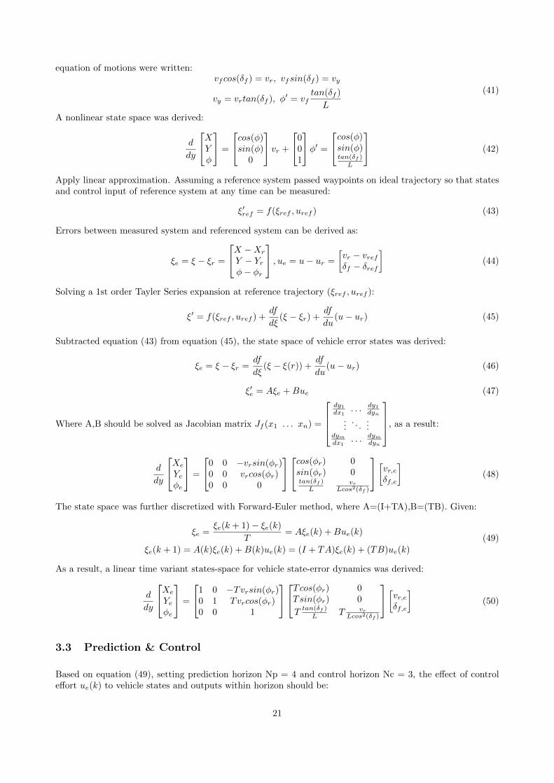
Based on Jianwei Qiu (2014) [11], quadprog solver in MATLAB was applied to generate results in Figure 22.Red-dot trajectory indicated that vehicle was able to track straight line closely at all speeds. Blue line wasgenerated as the vector of U at each time steps. An offset of 1.5 m and heading angle 60 degrees were manuallyintroduced assuming vehicle could not start right on the track center. It was observed from Figure 22 thatlarge speed and steering was required at beginning to correct the trajectory. With a higher speed or largerheading error, trajectory might overshoot but eventually converge.
Figure 22: Trajectory Tracking for Straight Line
On curved trajectory, error occurred with naive controller at higher speed. Index of Q matrix was set as higherpriority to penalize large deviation from reference track. Hence on Figure 23, a spike of 1.7 rad/s yaw ratewas requested from steering to correct Y position error at T = 1 second. Algebraic-Riccati Equation could besolved to define Q matrix. It was also applicable to tune the index’s order of magnitude to be (1/error). Forexample, QX = QY = 100 was expected to bring position error down to 0.01m. R matrix should be tuned forsmoother control effort with a trade-off on position.
Note that a longer prediction and control horizon were beneficial for performance only below a threshold.Time complexities of optimizations should be evaluated in code. From simulation a bifurcation of trajectorieswas observed in the end. One possible reason was that the last waypoint had been detected at X = 7m, so alltrajectories were planned towards the point when approaching. Such behavior might not affect vehicle maneu-ver and should not exist on a close-loop track map. For next iteration effects of time should be incorporatedto improve the tracking precision.
23

Figure 23: Trajectory Tracking Curve with Penalized Error State
4 Hardware Implementation
4.1 System Identification
An experimental method to determine motor dynamic characteristic was system identification. Multiple torquecommands were applied to motor and corresponding steady states rotational speeds were measured. With lin-earity examined, slopes of the fitting lines were the damping coefficients of motors. As shown in figure,damping coefficients were 0.1595 on the left and 0.1997 on the right. The difference was a result of manu-facturing quality. Moreover, an impulse response test could determine the motor system bandwidth. Motorswere first driven to a constant torque output. Current, voltage, RPM and torque data were recorded as soonas torque commends stepped to zero and torque output ramped down. Given the bode plot of this process,motor transfer functions could be established accordingly.
24
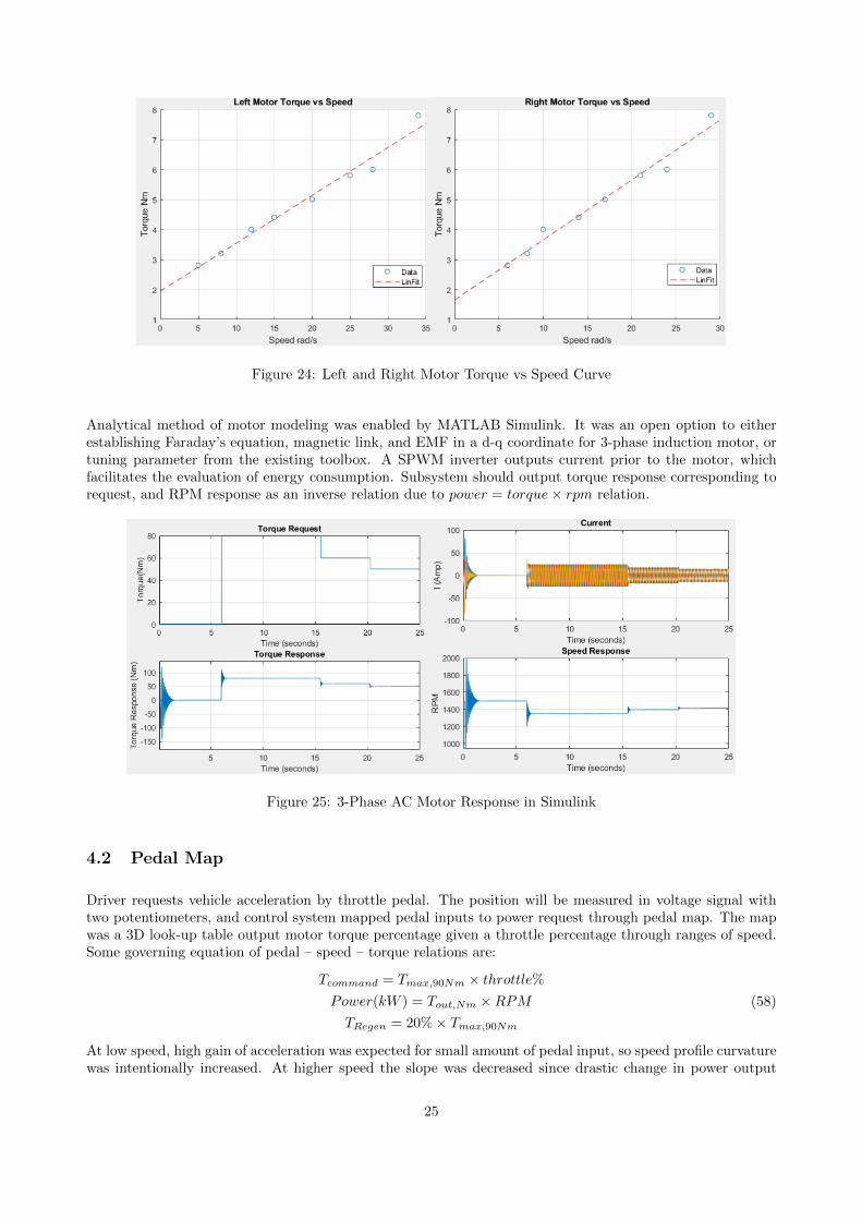
Figure 24: Left and Right Motor Torque vs Speed Curve
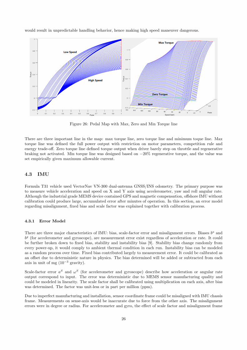
Analytical method of motor modeling was enabled by MATLAB Simulink. It was an open option to eitherestablishing Faraday’s equation, magnetic link, and EMF in a d-q coordinate for 3-phase induction motor, ortuning parameter from the existing toolbox. A SPWM inverter outputs current prior to the motor, whichfacilitates the evaluation of energy consumption. Subsystem should output torque response corresponding torequest, and RPM response as an inverse relation due to power = torque× rpm relation.
Figure 25: 3-Phase AC Motor Response in Simulink
4.2 Pedal Map
Driver requests vehicle acceleration by throttle pedal. The position will be measured in voltage signal withtwo potentiometers, and control system mapped pedal inputs to power request through pedal map. The mapwas a 3D look-up table output motor torque percentage given a throttle percentage through ranges of speed.Some governing equation of pedal – speed – torque relations are:
Tcommand = Tmax,90Nm × throttle%Power(kW ) = Tout,Nm ×RPMTRegen = 20%× Tmax,90Nm
(58)
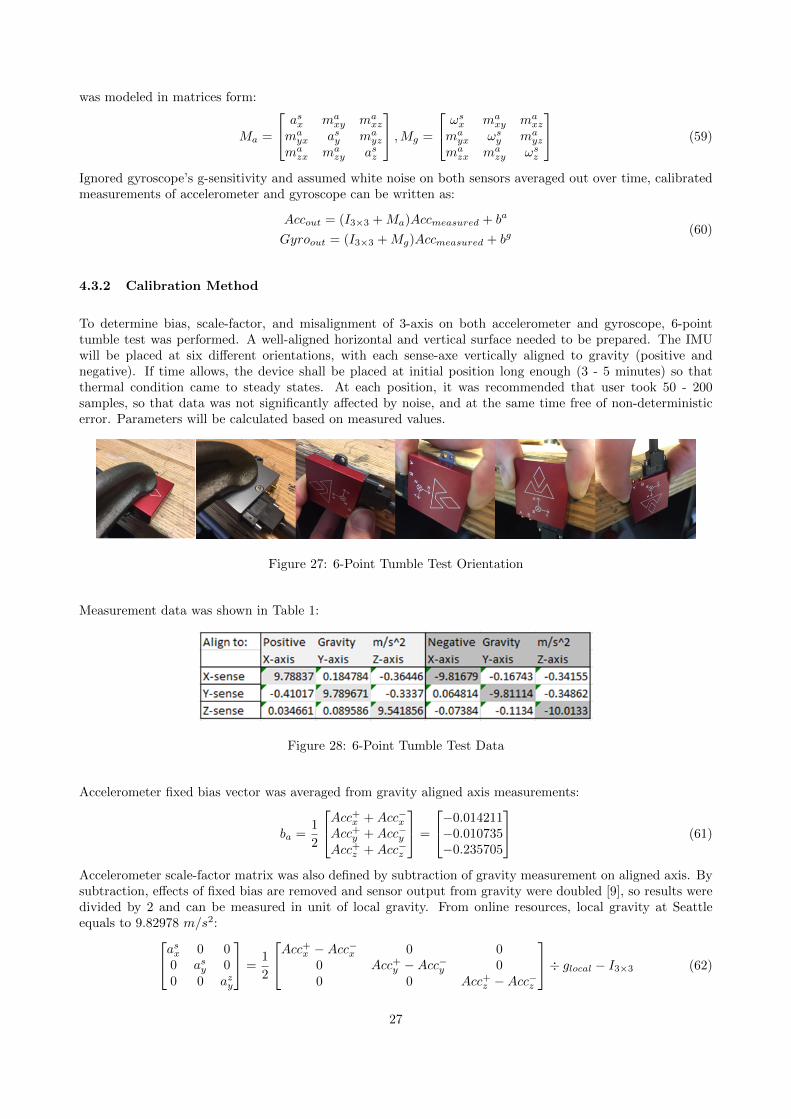
At low speed, high gain of acceleration was expected for small amount of pedal input, so speed profile curvaturewas intentionally increased. At higher speed the slope was decreased since drastic change in power output
25
would result in unpredictable handling behavior, hence making high speed maneuver dangerous.
Figure 26: Pedal Map with Max, Zero and Min Torque line
There are three important line in the map: max torque line, zero torque line and minimum toque line. Maxtorque line was defined the full power output with restriction on motor parameters, competition rule andenergy trade-off. Zero torque line defined torque output when driver barely step on throttle and regenerativebraking not activated. Min torque line was designed based on −20% regenerative torque, and the value wasset empirically given maximum allowable current.
4.3 IMU
Formula T31 vehicle used VectorNav VN-300 dual-antenna GNSS/INS odometry. The primary purpose wasto measure vehicle acceleration and speed on X and Y axis using accelerometer, yaw and roll angular rate.Although the industrial grade MEMS device contained GPS and magnetic compensation, offshore IMU withoutcalibration could produce large, accumulated error after minutes of operation. In this section, an error modelregarding misalignment, fixed bias and scale factor was explained together with calibration process.
4.3.1 Error Model
There are three major characteristics of IMU: bias, scale-factor error and misalignment errors. Biases ba andbg (for accelerometer and gyroscope), are measurement error exist regardless of acceleration or rate. It couldbe further broken down to fixed bias, stability and instability bias [9]. Stability bias change randomly fromevery power-up, it would comply to ambient thermal condition in each run. Instability bias can be modeledas a random process over time. Fixed bias contributed largely to measurement error. It could be calibrated asan offset due to deterministic nature in physics. The bias determined will be added or subtracted from eachaxis in unit of mg (10−3 gravity).
Scale-factor error aS and ωS (for accelerometer and gyroscope) describe how acceleration or angular rateoutput correspond to input. The error was deterministic due to MEMS sensor manufacturing quality andcould be modeled in linearity. The scale factor shall be calibrated using multiplication on each axis, after biaswas determined. The factor was unit-less or in part per million (ppm).
Due to imperfect manufacturing and installation, sensor coordinate frame could be misaligned with IMU chassisframe. Measurements on sense-axis would be inaccurate due to force from the other axis. The misalignmenterrors were in degree or radius. For accelerometer and gyro, the effect of scale factor and misalignment frame
26
was modeled in matrices form:
Ma =
asx maxy ma
xz
mayx asy ma
yz
mazx ma
zy asz
,Mg =
ωsx maxy ma
xz
mayx ωsy ma
yz
mazx ma
zy ωsz
(59)
Ignored gyroscope’s g-sensitivity and assumed white noise on both sensors averaged out over time, calibratedmeasurements of accelerometer and gyroscope can be written as:
Accout = (I3×3 +Ma)Accmeasured + ba
Gyroout = (I3×3 +Mg)Accmeasured + bg(60)
4.3.2 Calibration Method
To determine bias, scale-factor, and misalignment of 3-axis on both accelerometer and gyroscope, 6-pointtumble test was performed. A well-aligned horizontal and vertical surface needed to be prepared. The IMUwill be placed at six different orientations, with each sense-axe vertically aligned to gravity (positive andnegative). If time allows, the device shall be placed at initial position long enough (3 - 5 minutes) so thatthermal condition came to steady states. At each position, it was recommended that user took 50 - 200samples, so that data was not significantly affected by noise, and at the same time free of non-deterministicerror. Parameters will be calculated based on measured values.
Figure 27: 6-Point Tumble Test Orientation
Measurement data was shown in Table 1:
Figure 28: 6-Point Tumble Test Data
Accelerometer fixed bias vector was averaged from gravity aligned axis measurements:
ba =1
2
Acc+x +Acc−xAcc+y +Acc−yAcc+z +Acc−z
=
−0.014211−0.010735−0.235705
(61)
Accelerometer scale-factor matrix was also defined by subtraction of gravity measurement on aligned axis. Bysubtraction, effects of fixed bias are removed and sensor output from gravity were doubled [9], so results weredivided by 2 and can be measured in unit of local gravity. From online resources, local gravity at Seattleequals to 9.82978 m/s2:asx 0 0
0 asy 00 0 azy
=1
2
Acc+x −Acc−x 0 00 Acc+y −Acc−y 00 0 Acc+z −Acc−z
÷ glocal − I3×3 (62)
27
It can be solved that:asx = −0.00277, asy = −0.00299, asz = 0.00531 (gravity)
Accelerometer misalignment were calculated based on non-gravity axes measurements due to cross coupling.For the same reason results were divided by 2 and measured in local gravity: 0 ma
xy mxzamayx 0 ma
yz
mazx ma
zy 0
=1
2
0 Acc+y −Acc−y Acc+z −Acc−zAcc+x −Acc−x 0 Acc+z −Acc−zAcc+x −Acc−x Acc+y −Acc−y 0
÷ glocalmayx = mxya,m
azx = mxza,m
azy = myza,
(63)
Note that misalignment angle of sensor and casing are small and ignorable compared to misalignment whenbeing installed on the car.
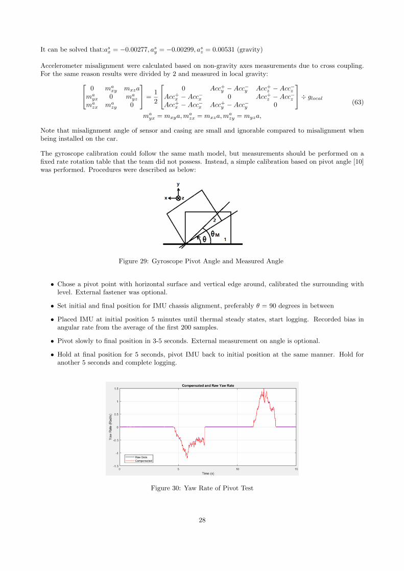
The gyroscope calibration could follow the same math model, but measurements should be performed on afixed rate rotation table that the team did not possess. Instead, a simple calibration based on pivot angle [10]was performed. Procedures were described as below:
Figure 29: Gyroscope Pivot Angle and Measured Angle
• Chose a pivot point with horizontal surface and vertical edge around, calibrated the surrounding withlevel. External fastener was optional.
• Set initial and final position for IMU chassis alignment, preferably θ = 90 degrees in between
• Placed IMU at initial position 5 minutes until thermal steady states, start logging. Recorded bias inangular rate from the average of the first 200 samples.
• Pivot slowly to final position in 3-5 seconds. External measurement on angle is optional.
• Hold at final position for 5 seconds, pivot IMU back to initial position at the same manner. Hold foranother 5 seconds and complete logging.
Figure 30: Yaw Rate of Pivot Test
28

Based on averaged yaw rate at first 200 sample, the offset bias error of gyroscope Z axis is: 0.003865 rad/s,comply to manual accuracy. By integrating uncompensated angular rate from 4 - 9 seconds, a rotation angleabout 120 degrees were calculated. Scale-factor error were defined as:
average(
9∑t=4
ActualAngle
IntegrationResult) = 0.7271 (64)
VectorNav claimed to have built-in kalman filter that compensated for various readings, but its effectivenesshad been unclear. As shown in the following graph, optional output of filtered angular rate was close touncompensated rate within 15 seconds. With numerical integration, both angular rates resulted in angleprediction far from actual input. All rotational axis could be calibrated using method above.
Figure 31: Scale-Factor Error of Gyroscope with Integration
All errors for accelerometer and gyroscope shall be removed using VectorNav control center. Calibratingon-vehicle IMU on a flat ground during competition shall be the first task after boot-up. The accelerationcalibration was performed under 40 Hz and gyroscope under 80 Hz. When connected to serial CAN, frequencycould be tuned as long as maximum baud rate does not exceed 115200.
5 Conclusion and Outlook
In this paper the author examined a PID based feedforward/feedback control to improve vehicle handlingperformance. A simulation of NMPC algorithm was performed as the skeleton when UWFM progressingtoward L2 autonomous driving. Yet the full potential of vehicle had not been explored. Here are some of thetopics that future members should investigate:
• Transient model of suspension should be investigated for riding analysis.
• System identification on roll dynamics should be performed to improve accuracy of normal force estima-tions. System identification of AC motor should be performed for FOC control.
• Understeer gradient should be measured by conducting constant radius experiments, on vehicle at openloop and with control. So that the handling limit can be quantitatively defined.
• Redundant sensors such as linear potentiometer on suspension and wireless torque control should beequipped for real-time feedback. A proper nonlinear kalman filter is needed on IMU.
• Vehicle models, and cost function for MPC should be well defined. Techniques such as pure-pursuit couldbe combined. Horizon and look-ahead distance should be optimized.
• When redesigning algorithm based on in-hub 4 motor powertrain, ground speed sensor may be requiredfor accurate vehicle speed estimation.
29
6 Acknowledgement
The author would like to express sincere gratitude to Romain, Cedric, Antonio and Ryan from University ofWashington Formula Motorsports. Special thanks to my committee for all the support to make this opportunityhappen.
References
[1] Nguyen,H.(2019) Traction Control and Torque Vectoring for the UWFM Electric Independent RWD VehicleKorper. University of Washington, 2019.
[2] Goran,v.,Bodan,S.(2016) Model Predictive Control Based Torque Vectoring Algorithm for Electric Car withIndependent Drives Korper. 2016 24th Mediterranean Conference on Control and Automation (MED), 2016.
[3] Leonardo De Novellis, Aldo Sorniotti, Ptrick Gruber, Andrew Pennnycott.(2014) Comparison ofFeedback Control Techniques for Torque Vectoring Control of Fully Electric Vehicles Korper. IEEE,10.1109/TVT.2014.2305475 2014
[4] Kun Jiang, Adina Pavelescu, Alessandro Correa Victorino, Ali Charara. Estimation of Vehicle’s Verti-cal and Lateral Tire Forces Consider Road Angle and Road Irregularityorper. 17th International IEEEConference on Intelligent Transportation Systems, Oct 2014.
[5] Antunes,J., Antunes,A. Outeriro,P. Cardeira,C. Oliveira,P.(2019) Testing of a Torque Vectoring Controllerfor a Formula Student Prototype, Robotics and Autonomous Systemsorper. Robotics and AutonomousSystems, March 2019.
[6] Wheals, J. Deane, M. Drury, S. Griffith, G et al.(2006) Design and Simulation of a Torque VectoringTMRear Axleorper. SAE Technical Paper 2006-01-0818,2006.
[7] Sawase,K., Ushiroda,Y.(2008) Improvement of Vehicle Dynamics by Right-and-Left Torque Vectoring Sys-tems in Various Drivetrainsorper. Misubishi Motors Technical Review, 2008
[8] Tedaldi,D., Pretto,A., Menegatti,E.(2014) A Robust and Easy to Implement Method for IMU CalibrationWithout External Equipmentorper. 2014 IEEE International Conference on Robotics Autonation, May 312014.
[9] Ferguson,J.(2015). Calibration of Deterministic IMU Errors orper. Embry-Riddle Aeronautical University,2015
[10] Looney,M.(2010) A Simple Calibration for MEMS Gyroscopes orper. Analog Device, EDN Europe July2010.
[11] Qiu,J.W., Jiang,Yan., Xu,Wei.,et al.(2014) Model Predictive Control for Self-driving Vehicles orper. Bei-jing Institute of Technology Press, April 2014.
[12] Schildbach,G.(2020) Vehicle Dynamics & Control YouTube Seriesorper. University of Luebeck, May 2020.
[13] Schouwenaars,T., How,J., Feron,E.(2004) Receding Horizon Path Planning with Implicit Safety Guaran-teesorper. American Control Conference, June 2004.
[14] Liniger,A., Domahidi,A., Morari,A.(2017) Optimization Based Autonomous Racing of 1:43 Scale RCCarsorper. Automatic Control Laboratory, ETH Zurich, 2017
[15] Liu,J., Jayakumar,P., Overhold,J.L., et al.(2013) The Role of Model Fidelity in Model Predictive ControlBased Hazard Avoidance in Unmanned Ground Vehicle Using LIDAR Sensors [C] orper. Proceeding ofASME Dynamic Systems and Control Conference, 2013:1-10.
[16] Cong,Y., An,X., Chen,H., et.al.(2012) Mobile Robotics Path Tracking Control Based on Receding Horizonorper. Jilin University, 2012.
30
7 Appendix
Symbols Variables Units
δ Steering Angle deg(rad)a,b Front Rear wheelbase mL Total wheelbase mR Instantaneous radius mm Vehicle mass Kgg Gravitation Constant 9.81m/s2
a Acceleration m/s2
Iz Yaw moment of inertia Kg ∗m2
Cf,r Cornering stiffness N/deg(N/rad)vx,y Long/Lat velocity m/sF Force Nφ Yaw angle Deg(rad)M Rotational momentum Nmα Slip angle Deg(rad)λ Slip ratio ratio
Wf,r Weight ratio ratioK Understeer gradient deg ∗ s2/mω Wheel speed RPM(rad/s)Rw Wheel radius mTf,r Trackwidth mµλ,α Frictional coefficient unitlessρair Air density Kg ∗m3
Ftr Traction force NTm Motor torque NmTb Damping torque NmJw Wheel assembly inertia Kg ∗m2
∆T Torque difference Nm
List of Figures
1 Mitsubishi Evo & S-AWC Yaw Control System . . . . . . . . . . . . . . . . . . . . . . . . . . . 6
2 CMU vehicle in DARPA Challenge . . . . . . . . . . . . . . . . . . . . . . . . . . . . . . . . . . 7
3 Cone Detection and SLAM in FSG . . . . . . . . . . . . . . . . . . . . . . . . . . . . . . . . . . 7
4 Vehicle Driver “Closed-Loop” System . . . . . . . . . . . . . . . . . . . . . . . . . . . . . . . . 8
5 Kinematic and Dynamic Bicycle Model . . . . . . . . . . . . . . . . . . . . . . . . . . . . . . . . 9
6 Understeer & Oversteer vs Slip Angle . . . . . . . . . . . . . . . . . . . . . . . . . . . . . . . . 11
7 Understeer & Oversteer vs Slip Angle . . . . . . . . . . . . . . . . . . . . . . . . . . . . . . . . 11
8 Characteristic Velocity and Critical Velocity . . . . . . . . . . . . . . . . . . . . . . . . . . . . . 12
9 Longitudinal Coefficient and Tire Force . . . . . . . . . . . . . . . . . . . . . . . . . . . . . . . 13
10 Longitudinal Coefficient at Different Slip Angle Given Friction Ellipse . . . . . . . . . . . . . . 14
31
11 Simplified Half Vehicle Wheel Dynamics . . . . . . . . . . . . . . . . . . . . . . . . . . . . . . . 15
12 Feedforward-Feedback Control Architecture . . . . . . . . . . . . . . . . . . . . . . . . . . . . . 16
13 Slip Ratio Response Open-Loop vs PI Control . . . . . . . . . . . . . . . . . . . . . . . . . . . . 17
14 Pole-Zero Map of System with PI Controller . . . . . . . . . . . . . . . . . . . . . . . . . . . . . 17
15 Wheel Speed and Controlled Slip Ratio in Straight Line Acceleration . . . . . . . . . . . . . . . 18
16 Motor Torque Output Comparison . . . . . . . . . . . . . . . . . . . . . . . . . . . . . . . . . . 18
17 Lateral Dynamics with Step Steer on Open Loop . . . . . . . . . . . . . . . . . . . . . . . . . . 18
18 Yaw Rate and Torque Distribution in with Torque Vectoring . . . . . . . . . . . . . . . . . . . 19
19 Safe Trajectory Library from Shouwenaars (2004) . . . . . . . . . . . . . . . . . . . . . . . . . . 20
20 Kinematic Bicycle Model for MPC . . . . . . . . . . . . . . . . . . . . . . . . . . . . . . . . . . 20
21 MPC Feedback Control Loop . . . . . . . . . . . . . . . . . . . . . . . . . . . . . . . . . . . . . 22
22 Trajectory Tracking for Straight Line . . . . . . . . . . . . . . . . . . . . . . . . . . . . . . . . 23
23 Trajectory Tracking Curve with Penalized Error State . . . . . . . . . . . . . . . . . . . . . . . 24
24 Left and Right Motor Torque vs Speed Curve . . . . . . . . . . . . . . . . . . . . . . . . . . . . 25
25 3-Phase AC Motor Response in Simulink . . . . . . . . . . . . . . . . . . . . . . . . . . . . . . . 25
26 Pedal Map with Max, Zero and Min Torque line . . . . . . . . . . . . . . . . . . . . . . . . . . 26
27 6-Point Tumble Test Orientation . . . . . . . . . . . . . . . . . . . . . . . . . . . . . . . . . . . 27
28 6-Point Tumble Test Data . . . . . . . . . . . . . . . . . . . . . . . . . . . . . . . . . . . . . . . 27
29 Gyroscope Pivot Angle and Measured Angle . . . . . . . . . . . . . . . . . . . . . . . . . . . . 28
30 Yaw Rate of Pivot Test . . . . . . . . . . . . . . . . . . . . . . . . . . . . . . . . . . . . . . . . 28
31 Scale-Factor Error of Gyroscope with Integration . . . . . . . . . . . . . . . . . . . . . . . . . . 29
32