DYNAMIC CLOUD SIMULATION USING

CELLULAR AUTOMATA AND TEXTURE SPLATTING

by

ERIC MAURICE UPCHURCH

B.S., University of Colorado at Colorado Springs, 2001

A thesis submitted to the Faculty of the Graduate School of the

University of Colorado at Colorado Springs

in partial fulfillment of the requirements for the degree of

Master of Science

Department of Computer Science

2009

2

This thesis entitled:Dynamic Cloud Simulation Using Cellular Automata and Texture Splatting

written by Eric Maurice Upchurchhas been approved for the Department of Computer Science

by

__________________________________Dr. Sudhansu Semwal

_________________________________________Dr. Tim Chamillard

__________________________________________Dr. C. Edward Chow

Date__________________

The final copy of this thesis has been examined by the signatories, and weFind that both the content and the form meet acceptable presentation standards

Of scholarly work in the above mentioned discipline.

3

Upchurch, Eric Maurice (M.S., Computer Science)

Dynamic Cloud Simulation Using Cellular Automata and Texture Splatting

Thesis directed by Professor Sudhansu K. Semwal

Visually convincing simulation of natural environments and natural phenomena has been a

goal of computer graphics for decades, and has broad applications in modeling environments and

entertainment venues, such as flight simulation, games, and film. This includes modeling of all sorts

of natural phenomena, ranging from water surfaces, fire, smoke, and clouds, to individual flora and

forests of trees.

Clouds in particular represent a challenge for modelers, since their formation, extinction, and

movement are amorphous and dynamic in nature. This project implements a computationally

inexpensive, real-time (or near real-time, depending on the hardware used) method for the simulation

of clouds using cellular automata, as put forth by Dobashi et al [9]. The model developed by Dobashi

is extended to incorporate cloud textures sampled from actual images of cloud systems. The

simulation model is also extended with an enhanced wind model for more organic cloud movement.

Furthermore, a graphical user interface for manipulating simulation and cloud model rendering

parameter values is provided, so that users may interactively control the simulation and its rendered

results.

4

ACKNOWLEDGMENTS

Many thanks to my graduate advisor, Dr. Sudhansu K. Semwal for helping me gain direction

for my project, and providing constant encouragement. Thanks to my wife Mindi for putting up with

long hours spent at the computer, always giving me time to work on my project, and always providing

the emotional support I needed.

5

CONTENTS

CHAPTER

INTRODUCTION.............................................................................................................................2

BACKGROUND................................................................................................................................2

Cloud Growth........................................................................................................................2

Cellular Automata.................................................................................................................2

PREVIOUS WORK..........................................................................................................................2

METHODOLOGY............................................................................................................................2

SIMULATION METHOD................................................................................................................2

Cloud Growth........................................................................................................................2

Cloud Extinction...................................................................................................................2

Controlling Clouds with Ellipsoids.......................................................................................2

Cloud Advection by Wind....................................................................................................2

RENDERING.....................................................................................................................................2

Continuous Density Distribution...........................................................................................2

Splatting................................................................................................................................2

Billboarding...........................................................................................................................2

IMPLEMENTATION.......................................................................................................................2

Simulation.............................................................................................................................2

Rendering..............................................................................................................................2

Graphical User Interface.......................................................................................................2

RESULTS...........................................................................................................................................2

6

CONCLUSIONS................................................................................................................................2

BIBLIOGRAPHY..............................................................................................................................2

7

TABLES

Table 1. Rendering frame rate results.......................................................................................................2

8

FIGURES

Figure 1. Air ascension caused by atmospheric thermal currents created by convection .......................2

Figure 2. Two-dimensional cellular automaton displaying regular but organic patterns..........................2

Figure 3. Conus textile shell exhibits a cellular automaton pattern..........................................................2

Figure 4. Example of Gardner's cloud rendering using 2D background textures and ellipsoids .............2

Figure 5. Cellular automaton representing voxels in 3D volume.............................................................2

Figure 6. Rendering process, smoothing binary to continuous density distribution.................................2

Figure 7. Basic cloud simulation transition rules......................................................................................2

Figure 8. Cloud simulation state transitions..............................................................................................2

Figure 9. Cloud simulation with control probabilities set too high...........................................................2

Figure 10. Pictoral view of Wyvill's field function...................................................................................2

Figure 11. Volume rendering by splatting................................................................................................2

Figure 12. Collective versus individual billboarding................................................................................2

Figure 13. Calculating billboard orientation.............................................................................................2

Figure 14. Simulation graphical user interface.........................................................................................2

Figure 15. Examples of different textures used on the same cellular automaton system.........................2

Figure 16. Cloud evolution through multiple time steps in a single cloud simulation.............................2

Figure 17. Cloud renderings produced by Dobashi et al...........................................................................2

9

CHAPTER I

INTRODUCTION

Algorithmic simulation of natural environments in a convincing manner is an open problem in

the realm of computer graphics, and presents an ongoing challenge to modelers and developers. The

ultimate goal is to present a computer-generated artificial environment that is indistinguishable from a

photographed natural landscape which, at the same time, is completely interactive in real-time. As

computer graphics hardware becomes more sophisticated, developers are reaching ever closer to this

goal. Of particular challenge in simulating natural environments is the dynamic creation and

animation of clouds.

Clouds are a ubiquitous feature of the earth and our everyday lives, and an important

component of the visual simulation of any outdoor scene. They provide a dynamic backdrop to the

outdoors, creating an infinite variety of shapes and patterns, and dramatically altering lighting

conditions in an environment. Because clouds constantly evolve into new shapes, or dissipate

completely, they also have a dramatic effect on outdoor scenes over time. The complexity of their

physical and visual properties has made clouds an important area of study in fields as diverse as

meteorology, physics, modeling and simulation, and computer gaming.

Clouds are complex phenomena that can be greatly affected by many different variables, at

both micro and macro levels. The dynamics of cloud formation, growth, motion and dissipation are

governed by many physical properties, including fluid dynamics, thermodynamics, and buoyant forces.

The complex physical nature of clouds makes simulation and rendering of cloud animations difficult in

real-time.

Several different methods of cloud generation have been proposed [1][6][14][29][31][32][35].

Many of these methods produce extremely realistic cloud images, but the images generated are static in

nature. In order to produce animations of clouds, some type of simulation component is needed for

dynamically changing the cloud system. Furthermore, since cloud color and shape changes based upon

10

the position of the sun and the viewer, as well as reflected light within a scene, the density distribution

of clouds needs to be defined in three-dimensional space in order to create realistic images.

One approach to creating realistic cloud animation is to simulate the physical phenomena.

This has proven, however, to be computationally intensive, and therefore does not lend itself well to

real-time applications. Thus, a simplified and computationally efficient method is needed, while still

maintaining a visually convincing result. To this end, this project expands upon a method of cloud

simulation put forth by Dobashi et al [9]. In this method, a three-dimensional cellular automaton is

employed as the simulation space. A set of simple cell transition rules, originally developed by Nagel

in [27], and a set of stochastic processes are utilized to simulate cloud formation, extinction, and

advection by wind.

This method of simulation is not sufficient if a user needs physically exact cloud motion, as it

only approximates the dynamics of clouds instead of modeling them directly. Instead, this simulation

technique allows us to approximate cloud shapes and motion without the need for computationally

expensive physical simulation. This is suitable for those who need a simple, computationally

inexpensive method to create cloud animations.

Dobashi’s method produces very good results, but there is always room for further

improvement to the technique. Our efforts aim to extend Dobashi’s simulation and rendering

techniques in several areas. First, we modified the rendering techniques used by Dobashi to

incorporate cloud textures captured from real images of clouds. These textures are then used as splats

upon the voxels represented by the cellular automaton employed by the simulation. Additionally, the

simulation includes an enhanced wind model, using user-defined functions to simulate wind vector

fields that alter the motion of the simulated cloud systems. In addition, all of the simulation and

rendering parameters are exposed through a graphical user interface (GUI) application. The GUI

provides a user the ability to alter simulation parameters with relative ease, and change rendering

parameters on the fly as the simulation results are used to generate the cloud images.

11

CHAPTER II

BACKGROUND

This section will cover some background material that is useful or important for

understanding the processes being simulated by this project, as well as how they are simulated. Details

on the actual simulation method will be covered in section .

Cloud Growth

The physical process of cloud formation within our atmosphere is quite a complicated

process. Clouds are comprised of liquid water droplets suspended within the atmosphere, not water

vapor as many people may think. The entire process begins with the presence of tiny particles within

the air, called cloud condensation nuclei (CCNs, also referred to as hygroscopic nuclei), upon which

water vapor can condense. Water requires such a non-gaseous surface upon which to make the

transition from vapor to liquid. Without such particles, the air would have to be supersaturated with

water vapor, at least several hundred percent relative humidity, in order for water droplets to

spontaneously form [17].

Next, the air must be saturated with water vapor (near 100% relative humidity). Water can

actually condense with lower levels of humidity if the air contains a high concentration of cloud

condensation nuclei. This is often the case in cities with severe air pollution, where pollution particles

act as CCNs, and can also occur during forest fires, where smoke particles act as CCNs. In fact, clouds

can be artificially seeded to grow by releasing fine particles into saturated air to catalyze the

condensation process [6].

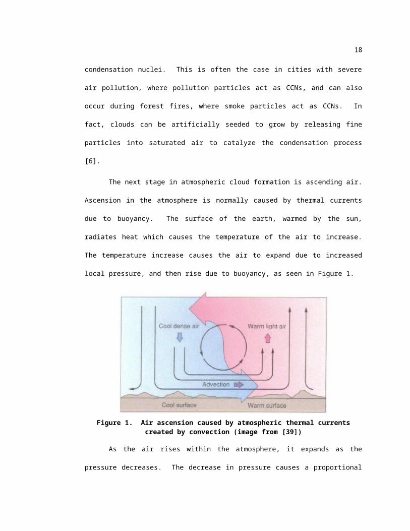
The next stage in atmospheric cloud formation is ascending air. Ascension in the atmosphere

is normally caused by thermal currents due to buoyancy. The surface of the earth, warmed by the sun,

radiates heat which causes the temperature of the air to increase. The temperature increase causes the

air to expand due to increased local pressure, and then rise due to buoyancy, as seen in Figure 1.

12

Figure 1. Air ascension caused by atmospheric thermal currents created by convection (image from [39])

As the air rises within the atmosphere, it expands as the pressure decreases. The decrease in

pressure causes a proportional decrease in temperature. Since cool air is able to contain less water

vapor than warm air, the decreased temperature results in an increase in relative humidity as a moist air

parcel rises. This, in turn, eventually leads to the rising air parcel reaching the point of saturation. The

temperature at which this process occurs is called the dew point.

Once the dew point has been reached, and if cloud condensation nuclei are present,

condensation of the water vapor will occur. This phenomenon is referred to as phase transition.

Furthermore, since the process of condensation is exothermic, it causes the release of latent heat of

condensation. This heat causes an additional increase in the temperature of nearby air, which in turn

increases its buoyancy, causing the air to rise even more. This is why many clouds seem to grow

upward. We believe cellular automata (described next) can provide one efficient platform for

simulating such an interaction.

Cellular Automata

A cellular automaton (CA) is a discrete dynamical model which consists of a regular grid or

lattice of cells (often referred to as the universe), each of which is in one of a finite number of states.

The grid can be specified in any finite number of dimensions – most generally in one, two, or three

dimensions. Time is also discrete, and the state of a cell at time step t is a function of the states of a

13

finite number of cells, called its neighborhood, at time step t − 1. The neighbors of a cell consist of a

selection of cells relative to the specified cell, and do not change.

A finite set of local transition rules are applied to cells in order to transition them to new

states. Transition rules specify how to update a cell’s state based upon the cell’s current state and the

states of the cell’s neighbors, as defined by its neighborhood. That is, the state of a cell at a given time

depends only on its own state one time step previously, and the states of its defined neighbors at the

previous time step. Every cell in the automaton has the same rules for updating, based upon the values

in this neighborhood. Each time the rules are applied to the entire grid of the cellular automaton, a

new generation is created. All cells on the lattice are updated synchronously. Thus, the state of the

entire lattice advances in discrete time steps. It is also feasible to use new updated values of

neighboring states easily, if desired.

The automaton does not have any input, and hence is autonomous. The collection of cell

states at any time point is called a configuration or global state of the CA, and describes the stage of

evolution of the CA. The initial state of the universe must be specified, and can sometimes (and

usually will) have a dramatic impact on the evolution of the CA. In general, the initial state consists of

having every cell in the universe placed in the same state, except for a finite number of cells in other

states. The initial configuration also commonly specifies that the universe starts out covered with a

periodic pattern, and only a finite number of cells violate that pattern. Furthermore, the configuration

may initially be set completely randomly. Henceforth after the initial configuration, the CA proceeds

deterministically under the effect of the transition rules, which are applied to each cell for every time

step.

Cellular automata were originally proposed by von Neumann as a means to generate self-

replicating systems. The main purpose of von Neumann was to bring the rigor of axiomatic and

deductive treatment to the study of “complicated” natural systems. The basic idea of a self-

reproducing automaton was presented by von Neumann as an adaptation of the idea of constructing a

universal Turing machine.

14

Figure 2. Two-dimensional cellular automaton displaying regular but organic patterns

Work on cellular automata within computing theory blossomed due to John Conway’s Game

of Life in the 1970’s, which used a two-dimensional, two-state CA. Despite its simplicity, the system

achieves an impressive diversity of behavior, fluctuating between apparent randomness and order.

Although originally viewed as a recreational topic, it has been shown that it is possible to arrange the

automaton so that the cells within the CA interact to perform computations, and can emulate a

universal Turing machine.

In 1983, Stephan Wolfram began publishing a series of papers that systematically studied a

basic class of cellular automata that were essentially unknown (an example is shown in Figure 2). The

unexpected complexity of the behavior of these simple cellular automata led Wolfram to suspect that

complexity in nature may be due to similar mechanisms. Indeed, similar patterns can be seen in

nature, such as the patterning present on the shell of Conus textile, as seen in Figure 3. Wolfram

published a treatise on his work, A New Kind of Science [41], in which he gives proof that certain CA

demonstrate the capability of universal computation. That is, these CA act as universal Turing

machines, capable of simulating any other Turing machine.

15

Figure 3. Conus textile shell exhibits a cellular automaton pattern

Cellular automata have since become an important tool in computational theory as well as

modeling and simulation. CA have been employed in computing topics as diverse as physical

modeling, data mining, random number generation, and networking. Cellular automata have been used

to model various physical processes, such as fire and smoke [7][12][20], clouds [9][27], landslides [5],

crack patterns [21], and material surfaces [11].

PREVIOUS WORK

Extensive research has been applied to the area of cloud modeling, both within the field of

computer science as well as meteorology. Both fields have had, and still have, active research in

methods for simulating, visualizing, and predicting clouds and other atmospheric phenomena.

Computer simulation of clouds has generally been implemented using mathematical models,

falling into one of two categories: physics-based simulation or procedural modeling. Physics-based

cloud simulation methods produce realistic images by approximating the physical processes within a

cloud. This involves computational simulation of fluid dynamics by solving Navier-Stokes equations,

or simplified models such as Stable Fluid and coupled map lattice (CML) [13][25][29][38]. A CML is

a mapping of continuous dynamic state values to nodes on a lattice that interact (i.e. coupled) with a set

of other nodes in the lattice according to specified rules [16]. Fluid dynamics simulations accurately

model the physical processes of cloud formation, whereas CML models, instead of solving for the

global behavior of a phenomenon, model the behavior by a number of very simple local operations.

16

When aggregated, these local operations produce a reasonably accurate representation of the desired

global behavior being simulated.

Fluid simulations produce some of the most convincing and realistic images of gaseous

phenomena, but are extremely computationally intensive. Large-scale and high-quality physics-based

simulation still exhausts all current commodity computational resources. This makes such simulation

approaches to cloud modeling a slow, offline process. Fine tuning of the models in such simulation

thus becomes difficult, and is a very slow iterative process. Due to the nature of the complexity of the

models, tweaking physical parameters may have no observable effect on the resulting images

produced, or may give rise to undesirable side-effects, including loss of precision and numeric

instability [36]. The complexity of physics-based models and their associated parameters also

introduces interfaces for manipulating the models that are cumbersome and non-intuitive for artists.

As such, rendering of the cloud models becomes a slow, tedious trial and error process. This is not to

say that such physical simulations are always slow. Simplifications of the physical process of cloud

evolution have resulted in some very convincing real-time simulations. In [17], Harris et al. present a

physically-based interactive cloud simulation that produces visually convincing results. Their system

models clouds using partial differential equations describing fluid motion, thermodynamic processes,

buoyant forces, and water phase transitions.

Procedural cloud models, on the other hand, rely on mathematical computations often

involving heuristics or stochastic processes such as volumetric implicit functions, fractals, Fourier

synthesis, and noise to create cloud-like structures [9][24][33][35]. Several early implementations of

cloud modeling were based upon the work by Perlin in [33]. Here, Perlin presented a method for

generating continuous random data within a volumetric space, based on using harmonics. This method

is referred to as Perlin noise, and has use in many applications, including fast cloud modeling for

gaming [34].

While these procedural models do not accurately represent the physical properties of clouds

such as formation and movement, they typically provide a much faster means of generating clouds, yet

maintain results that are visually convincing. Procedural modeling systems also generally produce

17

more controllable results than those of physics-based simulations [9]. Procedural models begin by

formulating the high-level structure of a cloud system, using methods such as fractal motion or cellular

automata [27][28][36]. The model is then used as the basis for a rendering scheme, which may use any

number of methods, such as fractals or particle systems. Often, clouds may be modeled initially as

rough volumetric ellipsoids, atop which detail is added procedurally using these modeling methods.

Once the cloud model is generated, it can be rendered in the context of an environment.

Dozens of rendering techniques have been used, with varying degrees of success in creating a realistic,

visually convincing image. Some early work on volume rendering with clouds was done by Blinn in

[1]. Blinn’s work attempted to accurately model light diffusion through clouds, accounting for

reflection, refraction, absorption and scattering by addressing the light interactions that occur when

light passes through a low-albedo particle cloud. Gardner used a combination of 2D and 3D

representations to create a cloud scene [14]. This method used a 2D texture to display high-level

clouds in the background, far away from the user viewpoint, while using 3D textured ellipsoids to

model foreground clouds (see Figure 4). This general method of combining 2D and 3D textures to

model clouds has also been used by others, such as Harris in [17], where cloud “imposters” are

rendered as 2D textures based on the current viewpoint, and swapped out for 3D volumes as the user

approaches the cloud in 3D space.

Correct lighting and shading is an essential component in producing visually convincing

cloud images and animations. Since clouds are partially translucent and refractive, lighting is an

extremely complex and difficult problem. In addition to light diffusion through clouds, which must

account for reflection, refraction, absorption, and scattering, some reflection of light occurs between

clouds, creating interdependency between separate cloud models. This can be handled using ray-

tracing techniques [22]. While ray tracing produces beautiful results with extremely accurate lighting,

such methods can be very time consuming and are not conducive to animation in real-time.

18

Figure 4. Example of Gardner's cloud rendering using 2D background textures and textured ellipsoids (image from [14])

Lighting calculations can be simplified, yet still produce convincing results in real time, as

seen with the approximate volumetric lighting model in [36]. Much of the recent research into

rendering methods for clouds and other volumetric data has focused on accounting for effects such as

skylight and atmospheric light attenuation. Dobashi presents an efficient method for rendering

volumetric cloud data based upon the density at each voxel in a volume [9]. His technique is based

upon the splatting method for volume rendering using billboards - 2D textured polygons whose normal

vectors always face the user. Here, he calculates the color of clouds taking into account the single

scattering of light. The color is computed by summing the scattered light reaching from the sun, the

attenuated light reaching from behind the clouds, and the color transmitted from the sky. Dobashi’s

method is efficient for a relatively small number of voxels in a volumetric data set, but does not scale

well to larger systems, as it requires traversal of all of the volumetric data, with some voxels

potentially being traversed multiple times depending upon viewing angle.

Commercial modeling applications also have some support for modeling and animating

clouds. Most modeling programs, such as Autodesk Maya simulate clouds as a collection of particles.

Particles serve as placeholders for offline rendering of high quality cloud media, including high-

resolution cloud imposter textures. The modeler application renders the clouds by developing an

19

interrelation between particle and renderable regions by building up a dependency graph of attributes

and filters (referred to as a shader graph) and assigning numerous variables and bindings to each node

in the tree. This is a generic rendering technique that may be used for rendering any number of

models, including clouds, but the generality comes at a price – high quality renderings require offline

processing, and thus do not support real-time applications.

20

CHAPTER III

METHODOLOGY

Dobashi’s method for cloud simulation, as presented in [9], is used as the basis for simulating

cloud systems within this project. The simulation starts with a three-dimensional cellular automaton,

whereby each cell in the automaton represents a single voxel in the simulation space, as shown in

Figure 5.

Figure 5. Cellular automaton representing voxels in 3D volume (image from [9])

At each cell of the automaton, three logical variables – vapor/humidity (hum), cloud presence

(cld), and phase transition/activation (act) – are assigned. Since the variables are simple Booleans,

they have only two possible states: on (value of 1), or off (value of 0). Cloud evolution is then

simulated by applying a set of simple state transition rules at each time step, as originally specified by

Nagel in [27], and extended by Dobashi in [9]. The transition rules allow the system to simulate cloud

formation, extinction, and advection by wind. Since the states are stored as simple logical variables,

we can apply correspondingly simple and fast Boolean logic for state transitions. Furthermore, since

each variable can be stored in a single bit, the memory required is relatively low (three bits per cell for

each time step that we need to store), and the simulation process can be accomplished even faster using

bit manipulation functions available in almost all programming languages.

The simulation results serve as the basis for the rendering step, which occurs next. As a result

of running a simulation time step, we obtain a discrete binary distribution of cloud presence, where

21

each cell either has clouds (cld = 1), or does not have clouds (cld = 0). The discrete binary distribution

provides a rough shape of cloud structure, but for rendering purposes, we want a continuous

distribution. To accomplish this, we can smooth the binary distribution into a continuous density

distribution based upon cloud presence in neighboring cells, as shown in Figure 6. We can then use

volume rendering techniques to render the density distribution. For this project, we use 2D texture

billboarding techniques utilizing the density at each cell as the basis for the color, opacity, and of the

textured billboard.

Figure 6. Rendering process, smoothing binary to continuous density distribution (image from [9])

SIMULATION METHOD

This section will describe in detail the simulation method used for creating clouds. It will

detail the points of Nagel’s original method, Dobashi’s extensions, and the extensions created for this

project.

Cloud Growth

To simulate cloud growth, we use Nagel’s method, which employs a three-dimensional

cellular automaton to simulate the processes outlined in section . For simplicity, the lattice of the

cellular automaton is aligned parallel to the major axes (x, y, z) in three-dimensional space. The

number of cells is then defined as nx× ny× nz. As previously mentioned, three logical variables, hum,

act, and cld are assigned at each cell (Figure 5). The state of each variable is either 0 or 1; hum=1

represents the presence of enough vapor to form a cloud, act=1 specifies that phase transition from

vapor to water droplets is ready to occur, and cld=1 specifies the presence of water droplets (that is,

clouds).

22

If we represent the states of each cell located at spatial coordinates (i, j, k) as a function of the

time step t, then the three basic transition rules for the cellular automata are given below, and are

summarized in Figure 7. In the formulae for the rules, A⋀B and A∨B represent logical

conjunction (i.e. AND), and logical disjunction (i.e. OR) operations between A and B. Similarly, ¬A

indicates negation (i.e. NOT) of A.

humijk ( t+1 )=humijk (t )∧¬ actijk (t) (1)

cld ijk ( t+1 )=cldijk( t)∨ act ijk(t) (2)

act ijk ( t+1 )=¬act ijk( t)∧humijk (t )∧f act(i , j , k) (3)

Here, fact is a Boolean operation that calculates its value based upon the phase transition state

(act) of a defined neighborhood around the cell. This function accounts for the fact that clouds grow

upward and outward by relying more on the phase transition state of cells above and beside the cell

than that of those below the cell.

f act (i , j , k )=act i+1 , j ,k ( t )∨ acti , j+1, k ( t )∨act i , j ,k +1(t)∨ act i−1, j , k (t )∨act i , j−1, k (t)∨act i , j ,k−1(t)∨acti−2 , j ,k (t )∨acti+2 , j ,k (t)∨acti , j ,k −2(t )∨ acti , j , k+2(t )∨act i , j−2 ,k (t )(4)

Dobashi et al. tried several variations of fact without significant differences in the generated

images, and thus used the original function as presented in equation (4). For this project, I also

experimented with several different options, including using diagonal neighbors, with no discernable

difference in output. Thus, the original function is also used for this project. The transition rules and

effects are summarized in Figure 7.

23

Figure 7. Basic cloud simulation transition rules (image from [9])

The rules are thus interpreted as follows. If there is currently enough humidity (hum=1) in a

cell, but phase transition has not yet occurred (act=0), then the cell remains humid. If there is enough

humidity in a cell (hum=1), but phase transition has not yet occurred (act=0), and phase transition has

occurred in one or more of the cell’s neighbors (fact =1), then phase transition occurs for that cell (act

becomes 1). This is displayed in the first row of Figure 7. After this, both act=1 and hum=1 for the

cell. Next, as displayed in the middle row of Figure 7, hum becomes 0, indicating that phase transition

is now ready to occur. Finally, when act=1, phase transition occurs, and clouds form at the cell (cld

becomes 1).

To initialize the cellular automaton, hum and act are randomly set using a pseudorandom

number generator (i.e. a coin flip), and cld is set to zero for all cells. Thus, the simulation starts with a

clear sky, and clouds form based upon updating the state of each cell using the rules presented above at

each time step. Furthermore, the cellular automaton’s simulation space is used as a boundary, where

all states are assumed to be zero outside of the CA’s lattice.

Cloud Extinction

As evidenced in formula (2), and shown in the bottom row of Figure 7, once the cld state

variable becomes 1, it remains 1 forever. Thus, cloud extinction never occurs. This is a distinct

24

disadvantage to Nagel’s method. In [9], Dobashi et al. introduced an extinction probability, pext, to deal

with this problem. This formulates a new transition rule, whereby a random draw is performed against

pext at each cell where cld=1. A random number, rnd in [0,1], is generated and checked against pext. If

rnd < pext, then cld is transitioned to 0. By changing pext at each cell at different times during the

simulation, we can control regions where cloud extinction occurs. While this provides cloud

extinction, it also introduces the converse problem. Once cloud extinction occurs at a given cell, it

never reforms. To solve this problem, Dobashi et al. also introduced similar rules for both

vapor/humidity (hum) and phase transition/activation (act). Thus, probability of vapor, phum, and

probability of phase transition, pact, are introduced in order to randomly re-seed these states into the

simulation. By controlling these probabilities, pext, phum, and pact, we can control cloud motion within

the simulation. The new transition rules are defined below.

cld ijk ( t+1 )=cldijk( t)∧ IS(rnd> pext (i , j , k , t )) (5)

humijk ( t+1 )=humijk (t)∨ IS (rnd> phum(i , j , k , t)) (6)

act ijk ( t+1 )=act ijk(t)∨ IS (rnd> pact (i , j , k , t)) (7)

Figure 8. Cloud simulation state transitions

Here, rnd is a uniform random number in [0,1], and IS(e) is a Boolean test function which

returns 1 if e is true, and 0 if e is false. Figure 8 summarizes the cloud evolution process as defined by

25

equations 1-8, and displays the lifecycle of cell states through the simulation process within the cellular

automaton.

Controlling Clouds with Ellipsoids

As mentioned previously, cloud motion can be controlled by controlling the vapor probability,

phum, phase transition probability, pact, and cloud extinction probability, pext. Defining these

probabilities can be accomplished in a number of manners, including ellipsoids [9] and meatball filters

[24]. Since cumulous clouds often have a generally ellipsoidal meta-structure, ellipsoids provide a

convenient model for calculating the probabilities. Ellipsoids roughly simulate wet air parcels,

whereby the vapor probability and phase transition probability are higher near the center of the

ellipsoid, and gradually approach zero near the edges. Inversely, since clouds dissipate from the edges

inward, the cloud extinction probability is higher at the edges and proportionately lower near the

center.

As in Dobashi’s work [9], we utilize ellipsoids to control the distribution of probability values

in the simulation space. Our method of computing the probability values is linear, based upon the

magnitude of the distance from the center of each ellipsoid to the location of each cell in the cellular

automaton. Other functions could be used to determine probability distribution within the ellipsoids.

It would be an interesting extension to allow the probability distribution function to be user-defined.

We limit the ellipsoid radii to be aligned along the global x, y, and z axes for convenience in

calculating probabilities for each cell. Furthermore, if multiple ellipsoids overlap, we short-circuit

probability calculation for cells within the intersection such that the first ellipsoid processed defines the

probabilities for that cell.

Controlling the ellipsoid parameters, such as the radii, position, and function for calculating

state probabilities, allows us to generate different resulting cloud structures. This could potentially be

used to generate different types of clouds, though the cellular automaton transition rules are primarily

oriented at producing cumulous-type cloud structures.

26

Cloud Advection by Wind

Wind can have a dramatic effect on cloud motion, often completely changing the structure of

a cloud by altering different sections of the cloud in different directions. Dobashi et al. introduced a

new set of transition rules for the cellular automaton to simulate a simple wind effect [9]. In their

method, the cells in the automaton are simply shifted in the wind’s direction, which is always assumed

to be the global x-axis. Additionally, wind velocity in their method is determined linearly as a function

of height of a cell within the CA lattice (that is, v(yk)=c∙yk). While this method works quite well, it is

also limited, and extending it for multiple wind vectors becomes cumbersome in implementation due

to the shifting of cell states that must occur.

In this project, we take a different approach to both wind definition and how wind affects the

simulation. Instead of shifting cells within the CA directly to achieve wind movement, our simulation

shifts the ellipsoids that define the distribution of vapor probability, phum, phase transition probability,

pact, and cloud extinction probability, pext. Thus, the probability distributions are constantly in flux

based upon winds defined as simulation parameters. This provides a great deal of control over cloud

movement, and is easily extendable to handle multiple wind functions – not only in the y-direction, but

in any direction within three-dimensional space.

Two different approaches may be used for calculation of the probabilities at each cell. The

first approach is to dynamically calculate the probability at each cell during each time step of the

cellular automaton, when the transition rules are applied. This requires intersection testing with the

ellipsoids in order to find the ellipsoid which contains the cell (if indeed any of the ellipsoids actually

contain the cell). This can be accomplished by using an octree data structure in order to quickly

determine which ellipsoids are in the same general area as the cell, and then only testing for cell

inclusion within those ellipsoids. Since octrees provide an efficient and fast means for

sorting/traversal of three-dimensional spatial data, this approach would scale well to larger cellular

automata grids, as the octree can be searched in O(NlogN) time.

An alternate method of calculating the probabilities is to pre-process the ellipsoids, storing the

values of pext, phum, and pact at each cell location. This then makes probability lookup trivial, as it

27

becomes a simple (and fast) array access. However, this method has the distinct disadvantage of being

much more memory intensive than the previously described method, since we must store three floating

point numbers, one for each probability factor (4 bytes each), for each cell in the CA. With current

computing hardware levels, memory is inexpensive and abundant, so this is not a large issue. For

example, a CA lattice of 256×256×32 cells would consume 24 megabytes of memory for probability

storage. However, it should be noted that this method will not scale well to very large CA lattices, as

the memory requirement increases accordingly (i.e. if we have N cells in the CA, then the memory

required is O(N)). Since this project deals with CA lattices that are near this size, this method was

deemed adequate, and is used in the project implementation.

To compute the probabilities, the application uses a simple ellipsoid traversal. We loop

through each of the defined ellipsoids and, leveraging the constraint that ellipsoids are axis-aligned

with the global xyz axes, get the bounding box of the ellipsoid. We then go through each integral index

within the bounding box, which corresponds to a cell in the CA, and compute and store the

probabilities at that index. Probabilities are computed linearly based upon the distance from the CA

cell to the center of the ellipsoid.

Figure 9. Cloud simulation with control probabilities set too high

28

During project implementation, it was found that the raw probabilities (simply calculating the

previously mentioned ratio) were far too high for pext, phum, and pact. Use of the raw probabilities

without any adjustment cause the clouds to become far too dense, and cells transition to clouds (cld=1)

nearly all of the time. As a result, the simulation effectively just volumetrically fills all of the

ellipsoids. This results an unnatural, “puff-ball” cloud structure, as shown in Figure 9. To alleviate

this issue, our simulation utilizes a user-definable scalar dampening factor for each of the probabilities

(pext, phum, and pact) that are multiplied against the calculated probability to adjust the probability used to

a reasonable level. Users can adjust these dampening factors to achieve different simulation results.

By setting the dampening factors higher, clouds become more puffy and full, whereas setting the

dampening factors lower results in more sparse, wispy cloud structures.

RENDERING

Cloud rendering can be accomplished in dozens of manners, from use of 2D or 3D texturing

to complex volume rendering techniques which take into account multiple scattering of light due to the

albedo of water droplets in the air. Dobashi et al. in [9] use a volume rendering technique known as

splatting to accumulate color information at each voxel in the simulated system based upon the density

at each cell, and the amount of light passing through each cell along rays cast from the view plane

through the cellular automaton’s cells.

For rendering of our simulated clouds, we treat the cellular automaton simulation results as a

particle system, and use 2D texture billboarding, with color and opacity values defined based upon a

density distribution which is calculated from the simulation results. For texturing, we use real images

of clouds captured in digital photographs, with the sky color removed and replaced with a transparency

layer.

Continuous Density Distribution

At the end of each time step, our simulation produces a distribution of cloud presence among

the cells of the cellular automaton lattice. This distribution is discrete and binary, having only one of

two values – either 0 (no clouds) or 1 (clouds). However, in the real world, clouds are comprised of a

29

continuous density distribution with values ranging from 0 to 1. This continuous change in density

among a cloud’s structure is what uniquely defines the appearance of a cloud. In order to smooth the

simulation’s discrete distribution into a continuous one, we utilize the smoothing method put forth by

Dobashi et al. in [9], and described here.

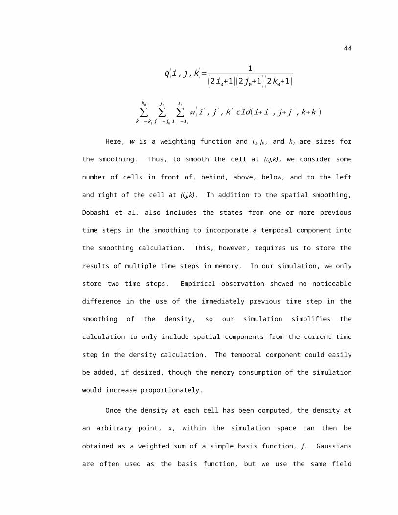
To begin, we calculate the density, q(i,j,k) at each cell (i,j,k) within the cellular automaton.

This is accomplished by considering the presence or absence of clouds in neighboring cells along the x,

y, and z directions from a cell. Thus, the density at each cell is computed as:

q (i , j , k )= 1(2 i0+1 ) (2 j0+1 ) (2k0+1 )

∑k '=−k0

k0

∑j'=− j0

j0

∑i'=−i0

i0

w (i' , j' , k ' ) cld (i+i' , j+ j' , k+k ')

Here, w is a weighting function and i0, j0, and k0 are sizes for the smoothing. Thus, to smooth

the cell at (i,j,k), we consider some number of cells in front of, behind, above, below, and to the left

and right of the cell at (i,j,k). In addition to the spatial smoothing, Dobashi et al. also includes the

states from one or more previous time steps in the smoothing to incorporate a temporal component into

the smoothing calculation. This, however, requires us to store the results of multiple time steps in

memory. In our simulation, we only store two time steps. Empirical observation showed no

noticeable difference in the use of the immediately previous time step in the smoothing of the density,

so our simulation simplifies the calculation to only include spatial components from the current time

step in the density calculation. The temporal component could easily be added, if desired, though the

memory consumption of the simulation would increase proportionately.

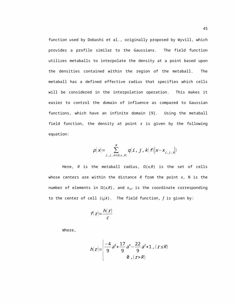
Once the density at each cell has been computed, the density at an arbitrary point, x, within

the simulation space can then be obtained as a weighted sum of a simple basis function, f. Gaussians

are often used as the basis function, but we use the same field function used by Dobashi et al.,

originally proposed by Wyvill, which provides a profile similar to the Gaussians. The field function

utilizes metaballs to interpolate the density at a point based upon the densities contained within the

30

region of the metaball. The metaball has a defined effective radius that specifies which cells will be

considered in the interpolation operation. This makes it easier to control the domain of influence as

compared to Gaussian functions, which have an infinite domain [9]. Using the metaball field function,

the density at point x is given by the following equation:

ρ ( x )= ∑i , j ,k∈Ω (x , R)

N

q ( i , j , k ) f (|x−x i , j ,k|)

Here, R is the metaball radius, Ω(x,R) is the set of cells whose centers are within the distance

R from the point x, N is the number of elements in Ω(x,R), and xi,j,k is the coordinate corresponding to

the center of cell (i,j,k). The field function, f is given by:

f (r )=h(r )c

Where,

h (r )={−49

a6+179

a4−229

a2+1 ,(r ≤ R)

0 ,(r>R)

a= rR

c=748405

πR

Here, r is the distance from the center of the metaball to the calculation point; in our case,

r=|x−x i , j ,k|. The constant divisor, c, is used to normalize the result (for derivation and details, see

[9] and [43]). Pictorially, the use of the field function is shown in Figure 10.

31

Figure 10. Pictoral view of Wyvill's field function used to smooth density distribution in simulation

Splatting

Once the smoothed density distribution has been calculated, we then proceed to render the

results. For rendering to the screen, Dobashi et al. use a splatting technique combined with billboards

[9].

Splatting is an object-order rendering technique whereby the volume being rendered is

decomposed into a set of basis functions, or kernels, which are individually projected onto the screen

plane in order to assemble an image [23]. We can consider the volume as a field of basis functions, h,

with one such basis kernel located at each grid point within the volume. The kernel is modulated by

the grid point’s value, and the ensemble of modulated basis functions comprises the continuous object

representation (see Figure 11). One can then interpolate a value at an arbitrary location within the

volume by adding up the contributions of the modulated kernels which overlap at that location. This is

the same idea as presented in the previous section, whereby we interpolate the density at an arbitrary

point within the volume based upon a metaball basis function. Thus, the density distribution serves as

the basis function used for splatting in Dobashi’s technique.

32

Figure 11. Volume rendering by splatting

Dobashi et al. use the splatting technique to acquire a texture based upon the density

distribution within each metaball, and the light passing through it. They take into account the light

reaching from the sun to the viewpoint through the density distribution, as well as the attenuated light

reaching from behind the clouds. Using this, the color of a voxel within the rendering volume is a

combination of the sun’s color, scattered along the viewing ray, the transmitted color of the sky behind

the clouds, and the attenuation of light through cloud particles.

Because we have a continuous density distribution, the attenuated light passing through each

metaball will have a different value, and will thus result in production of a different texture.

Implementing this would require a large amount of memory, proportional to the number of metaballs

used to render the volume. As a result, Dobashi discretizes the density into nq levels, and thus uses

only nq individual textures (64 in their case). The texture corresponding to the nearest density value is

then used for each metaball. Once the texture for each metaball is obtained, it is placed onto a

billboard, and the splatting algorithm is used to composite them into the viewing plane, producing the

image as viewed on screen.

Billboarding

In order to project textures onto the screen in the splatting algorithm, the textures must be

oriented so that their normal vectors face the viewpoint. This process is referred to as billboarding. A

billboard is simply a two-dimensional object, often a square, which always faces the viewer in a three-

dimensional scene. Dobashi et al. use texture-mapped billboards indirectly in their rendering

camera cameraCollective Billboarding Individual Billboarding

33

algorithm by projecting them directly onto a frame buffer. In this project, we use textured billboards

directly as rendering primitives, and let the OpenGL graphics library composite them through

blending.

Billboards constantly change orientation within a scene as the user’s viewpoint changes, or

the billboarded object itself moves. To accomplish this change in orientation, one can use two types of

billboarding: point or axis. Point billboards, also commonly referred to as point sprites, are centered at

a point, and the billboard rotates about that central point to face the user. Axis billboards only rotate

around a defined axis to face the user. Axis billboards are easier to implement, but are limited in their

orientation, making them ineffective for use in scenes where the user has full freedom of movement.

Since our simulation allows six degrees of freedom, we utilize point billboards for rendering.

Point billboards can either be billboarded collectively or individually (see Figure 12).

Collective billboarding orients all billboards in one direction, using the inverse of the camera direction.

Collective billboarding is very fast, as only one transformation matrix is calculated, but has the issue

that objects start to look flat as they get closer to the edges of the screen. Individual billboards, on the

other hand, use a unique orientation based upon the location of the object, and thus always truly face

the user, regardless of the distance from the object to the camera.

Figure 12. Collective versus individual billboarding

not 90°up

Camera up vector

billboard

camera

look

right

34

Individual billboards require more computation time, since each object has a unique

transformation matrix. To compute the transformation matrix, we need to know the camera position,

the camera up vector, and the billboard position. These are used to calculate the local billboard’s axis

of rotation. The billboard look vector is calculated from the camera position and the billboard position.

The look vector is oriented from the billboard toward the camera:

l⃗ookbillboard=poscamera−posbillboard

Once we have the look vector, we need to calculate the up and right vector for the billboard.

To do this, we can use the camera up vector as the temporary up vector for the billboard. This works

because the final billboard up vector, the billboard look vector, and the camera up vector lie along the

plane that contains the camera and billboard locations, as shown in Figure 13. The plane also has a

normal equal to the billboard right vector.

With the billboard look vector and the camera up vector, we calculate the right vector by

taking the cross product of the two vectors:

¿⃗billboard=⃗upcamera×⃗look billboard

Finally, we calculate the up vector for the billboard with another cross product:

u⃗pbillboard=⃗look billboard × ¿⃗billboard

Figure 13. Calculating billboard orientation - all green vectors lie in the plane outlined in dark grey, as does the blue vector of the billboard. The red vector of the billboard is perpendicular to

this plane.

35

Once we have calculated the local coordinate system of the billboard, we utilize the vectors to

create a transformation matrix to orient the billboard to face the camera. With the vectors normalized,

we use the rule of orthogonal matrices to create a rotation matrix for the billboard:

[r1 u1 l1 px

r2 u2 l2 p y

r3 u3 l3 pz

0 0 0 1]

Here, r represents the right vector, u represents the up vector, l represents the look vector, and

p represents the billboard’s position in global coordinate space. This matrix effectively transforms the

billboard coordinate system into the global coordinate system, orienting the billboard toward the

camera.

36

CHAPTER IV

IMPLEMENTATION

The simulation software developed for the project is implemented using the Java

programming language. It features a graphical user interface that is built using the standard

Java/Swing user interface library, and uses a multi-threaded simulation engine to decouple the

simulation from the GUI and rendering. Rendering is accomplished using the Java OpenGL bindings

(JOGL).

Simulation

The simulation engine is multi-threaded, with the cellular automaton updates occurring in one

thread, and wind simulation taking place in another thread. Having multiple threads allows the CA

updates and wind calculations to be executed independently of each other, and in parallel (the amount

of parallelism is dependent upon the multi-processing capability of the host system). The thread

performing wind calculations processes the defined wind equations, and moves the controlling

ellipsoids accordingly. Once all ellipsoids have been moved based upon the wind definitions, the

probability of extinction (pext), probability of phase transition (pact), and probability of humidity (phum)

are recalculated for each cell in the CA lattice as described in section . This asynchronous update of

probabilities means that the CA will access whichever probability numbers are currently calculated and

stored. That is, depending upon the speed of the CA update versus the speed of the probability

calculations, it may access probability factors from a previous wind time step or the current wind time

step. In practice, this does not have a negative impact on the simulation results.

Wind equations in the simulation are defined as quadratic equations that move ellipsoids in

the x-direction based upon y-values of the ellipsoid centers, and can be specified to operate on a

specific range of y-values. Having such range values allow, for example, clouds higher in the CA to

move in a different direction than those lower in the CA. While the equations are currently limited to

the x-direction, this could easily be extended to include other directions as well. As the wind thread

37

processes the defined wind equations on the collection of ellipsoids, the ellipsoids may move

completely out of the simulation space (that is, the cellular automaton grid), and thus no longer have

any impact in the simulation. Furthermore, if there is any wind at all, eventually all ellipsoids will exit

the simulation space. To handle this, each ellipsoid is checked against the boundaries of the CA after

the wind has been processed. If the ellipsoid is no longer within the bounds of the CA, then it is

reintroduced to the simulation space. The current implementation randomly mutates the ellipsoid

(redefining the ellipsoid’s radii) and then translates the ellipsoid back within the CA bounds such that

it has random y and z coordinates, and the x-coordinate is such that the ellipsoid is completely

contained within the CA bounds, but its leading edge coincides with the leading edge of the CA. This

random re-introduction of the ellipsoids produces very good results, and generally keeps the cloud

density near to what was initially defined by the simulation parameters.

For the cellular automaton implementation, the simulation leverages the fact that the state

variables required for each cell in the cellular automaton represent Boolean values. Since these

variables may only have the value of 0 (false) or 1 (true), we can save memory by storing the variables

in bit fields. This idea was proposed by Dobashi et al. in [9], and is implemented here as well. Using

bit fields has two distinct advantages. First, it reduces the memory footprint required for the CA,

allowing us to run simulations with larger numbers of cells with a relatively low memory requirement.

Secondly, and perhaps more importantly, we can use fast bit manipulation functions provided by

nearly all high-level programming languages such as C, C++, and Java to implement the transition

rules.

Using this method, we can store all state variables in arrays of integers. Assume that m is the

bit length of an integer in the system being used for the simulation, that we have a cellular automaton

with nx× ny× nz cells, and we are storing nt time steps. We can then store each of the state variables as

integer arrays of the form:

∫ [⌈ nx

m⌉ ] [ny ] [nz ] [nt ]

38

We then have three parallel integer arrays: one array for cloud presence (cld), one for

vapor/humidity (hum), and one for phase transition/activation (act). Transition rules can then be

implemented using bit manipulation functions to process m cells at a time. This procedure results in

extremely fast and efficient computation for state transitions compared to processing logical variables

directly using Boolean operators.

Use of bit fields for the state variables introduces a difficulty when dealing with random

numbers generated to check against the probability factors pext, phum, and pact when implementing the

transition rules. The problem lies in the fact that random numbers need to be generated at each cell in

order to check against the probability factors at that cell for state transition rules. To get around this

issue, Dobashi et al. used a look-up table that stores several random bit sequences which obey the

probability i/np (i=0,…,np). These are then retrieved based upon the current simulation probability

factors, and utilized in the transition rules.

The thread that controls processing of the cellular automaton sleeps for a specified time step

delay, measured in milliseconds, which can be defined by the user. The thread which controls wind

movement also utilizes this time step delay as a factor in how long the wind thread sleeps. Thus, the

two threads run independently, but within the same time scale. This allows the simulation processing

to be sped up or slowed down, based upon user desire.

Rendering

Rendering of the cloud simulation results is performed using the OpenGL graphics library

through the Java OpenGL bindings (JOGL). The binary cloud distribution produced by the simulation

is smoothed into a continuous density distribution, as described in section . After this smoothing, the

rendering of the clouds is performed as if the cells within the cellular automaton are particles within a

particle system, and the particles are rendered as texture-mapped billboards.

Each cell which has a density greater than zero contributes to the scene, and is assigned a

texture from the pool of cloud image textures that the user has defined. The texture assigned is based

upon the position of the cell in the cellular automaton, so that we do not have to store in memory

39

which texture is used by each cell. The calculated density for the cell is used to determine the

billboard’s white color saturation, opacity, and size. So, if a cell has a high density value, it will

contribute a more opaque, whiter color, as well as a larger textured billboard. Blending is performed

by the OpenGL graphics library, using front-to-back color blending. This effectively implements the

splatting algorithm by attenuating the color contributed by each cell.

Simulation time steps can cause fairly large changes across the cellular automaton. While the

smoothing of binary cloud presence into a continuous density distribution helps smooth the generated

images, the changes in density between time steps causes animation of the rendered cloud system to

appear choppy. To alleviate this, and make the animation between time steps more fluid, we utilize

linear interpolation between the calculated densities at each cell at each time step. In order to calculate

the interpolated density, we store two density values – one from the previous time step, and one from

the current time step. We then vary a time factor, t, from 0 to 1, between subsequent time steps. In

this manner, the density at a given time, t, between simulation time steps is given as:

ρt=ρ0+t ( ρ1−ρ0 ) , t∈ [ 0..1 ]

Since the density defines the color saturation, opacity, and size of the billboards, the

interpolation of the density between time steps in turn interpolates these values. This results in a

smoother, more visually appealing transition of the clouds between simulation time steps.

OpenGL provides direct support of billboarding via the GL_POINT_SPRITE extension,

which was standardized in OpenGL 1.4. This extension allows you to draw a textured quad by sending

a single vertex through the graphics pipeline, which is much faster than sending all four vertices of the

quad (plus a normal vector for lighting). The quad is then automatically oriented to face the camera

viewpoint. This technique was implemented originally, but was found to be inadequate due to

constraints placed on point sprites by OpenGL. The first constraint is that point sprites are always

rendered based upon a fixed pixel size. This is a problem in a dynamic system, which allows freedom

of movement, since the perspective matrix is not applied to the point sprites, and thus they have no

distance attenuation based upon the viewer’s viewpoint. To alleviate this problem, OpenGL allows

40

you to define a distance attenuation equation to use on the point sprites via the point parameter

GL_POINT_DISTANCE_ATTENUATION. This works well, but upon using it, we immediately ran

into another issue. Apparently, OpenGL places a maximum pixel size on the point sprites, based upon

the maximum point rendering size supported by the graphics card and driver. This limitation was

insurmountable, as the maximum point size was far too small to be useful when zoomed in close to the

clouds being rendered. As a result, we implemented billboarding directly, as described in section .

Graphical User Interface

The application software developed for the project features a graphical user interface (GUI)

which provides user control over nearly all of the simulation and rendering parameters, as shown in

Figure 14. The user interface uses the model-view-controller (MVC) software design pattern, and the

design thus decouples the simulation from the user interface. A simulation model class stores all of the

pertinent parameter information for the simulation, which the user defines via the GUI.

Figure 14. Simulation graphical user interface

The graphical user interface is divided into two main sections: simulation/rendering parameter

input, and rendering area. The divider between the two sections can be moved to resize or completely

41

hide either section. The parameter input area features user inputs for the following simulation and

rendering parameters:

Cellular automaton dimensions (i.e. number of cells in the x, y, and z directions)

Probability dampener factors for pext, phum, and pact

Ellipsoids for controlling cloud structure

Wind equations that control ellipsoid movement

Simulation time-step delay

Render mode (user-defined cloud textures, generated texture, points by density, points by

cloud presence)

Scale factor for scaling the CA/cloud area when rendering

Billboard scale factor

Toggling of billboard interpolation between time steps

Time between interpolation steps

Color multiplier (used to dampen color based upon density of a cell)

Textures used for billboarding when rendering clouds

Toggling of ellipsoid rendering, cloud rendering, skybox rendering, and CA boundary

rendering

When the user changes a simulation parameter via the user interface, it is immediately stored

within the simulation model. The model is then used as the data provider for the simulation, and

provides accessor functions to retrieve the value of each of the simulation parameters. Once the user

has configured the simulation parameters as they wish, they simply click the “Start” button on the GUI

to begin the simulation. The results are then rendered directly within the same window using OpenGL,

allowing the user to immediately see results in an interactive fashion. Additionally, the user can

modify nearly all of the simulation and rendering parameters on the fly during a simulation run. The

only parameters that are not allowed to be changed during a simulation run are the cellular automaton

dimensions, which are statically set at the start of the simulation. The user can also pause the

simulation at any time by pushing the “Pause” button, or stop the simulation by pushing the “Stop”

button.

The user interface allows users to directly define probability controlling ellipsoids via a dialog

window, in which they enter the ellipsoid radii (along the x, y, and z directions) and center location.

The defined ellipsoids are displayed in a list widget, which allows the user to edit or delete selected

42

ellipsoids. When the user selects one or more ellipsoids, the rendering of those ellipsoids changes to

red to show the user which ellipsoids are currently selected. Additionally, a random ellipsoid

generator is provided, which allows the user to enter the number of ellipsoids they wish to generate,

and a minimum and maximum radius (used for all three spatial dimensions) to use for the generated

ellipsoids. The random ellipsoid generator will then create those random ellipsoids, ensuring that they

are fully contained within the currently defined bounds of the cellular automaton.

The user may define any number of quadratic wind equations to be used in simulating cloud

advection by wind. The equations modify the center x-position of ellipsoids as a function of the center

y-position of the ellipsoid, though this could easily be extended to handle other direction vectors in the

future. Equation coefficients, as well as the range of y-values to use for the equation, are defined via a

dialog window. The defined equations are then displayed in a list widget, which allows the user to edit

or delete selected equations.

Users can select any number of texture images to use for billboarding when rendering the

simulation results. The user interface provides a list widget which displays all of the currently defined

textures. A user can add new textures via a file browsing dialog, in which the user can traverse the file

system and choose one or more image files to utilize as textures. The rendering system currently

supports files in both portable network graphics (PNG) and graphics interchange format (GIF) formats.

Other image formats (such as the popular JPEG format) are not supported due to their lack of support

for transparency, which is essential for proper rendering. Users can double-click their mouse on

texture images in the list widget in order to see a preview screen, which displays the image on a sky-

colored background. Texture images can be dynamically added and removed during the simulation in

order to produce different rendering results. Texture images are assumed to already have their sky

coloring removed and replaced with a transparency layer. A useful extension to the user interface

would be the ability to crop and add transparency to images in order to produce adequate cloud

textures directly within the GUI, rather than requiring users to use a third-party graphics utility to

accomplish this.

43

The rendering section of the application window features a “skybox” which provides a sky-

like, gradient colored background against which the clouds are rendered. The rendering area provides

the user complete control over the three-dimensional environment via mouse and keyboard control.

The user may left-click and drag their mouse to rotate the scene, use the arrow keys to move about the

scene (alternatively, the user may also use the W, A, S, and D keys similar to many computer video

games), use the Page Up and Page Down keys for direct vertical movement within the scene, and use

the mouse wheel to zoom in and out of the scene.

The simulation application also features the ability to store the simulation parameter

definitions to a file for later use. The parameter definitions are stored in XML format, which allows

for easy parsing, extensibility, and human readability. Additionally, the user interface provides the

ability to toggle display of current rendering frames per second (FPS), display of current simulation

time step, and capture screenshots of either the entire application window, or just the rendering area, as

portable network graphics (PNG) images.

44

CHAPTER V

RESULTS

The simulation software was implemented and tested on a 2.4 GHz Intel Core2 Duo machine

with 3GB of RAM, and a NVidia GeForce GTX 260 graphics card with 896MB of video memory.

Real-time simulations were accomplished using cellular automaton sizes of up to 256x20x256 using

billboarding. Using OpenGL’s built in point sprites, the frame rate increases significantly, more than

doubling. This shows how relatively slow manual billboarding is. The time spent performing

billboarding calculations could potentially be reduced dramatically by offloading billboarding

calculations to the graphics card’s GPU by utilizing an OpenGL Shading Language (GLSL) vertex

shading program. Furthermore, the simulation rendering currently does not perform any culling of

hidden billboards, which would cut down on the amount of geometry processed by the graphics card,

which would also provide a performance increase.

Table 1. Rendering frame rate results

CA Size # Cells # Ellipsoids Frame Rate64x20x64 82K 25 70 fps

128x20x128 328K 50 35 fps256x20x256 1311K 100 15 fps

The simulation time steps, on average, consume 0.3 seconds of computation time with a

cellular automaton size of 256x20x256. This time includes the application of the transition rules as

well as the continuous density distribution computation. Computation of the probability tables for the

wind thread takes approximately 0.3 seconds on average utilizing 100 ellipsoids within a 256x20x256

cellular automaton. The computation time for the probability tables will vary in proportion to the

number of ellipsoids present.

Several rendering results are displayed in Figure 15 and Figure 16. Figure 15 shows the

effects of using different textures on the same simulation model. The cellular automaton state and all

45

simulation and rendering parameters are the same through this series of images, with the only

difference being the texture(s) used.

(a) Generated cloud texture (b) Nine different cloud textures

(c) Single cirrus cloud texture (d) Single stratocumulus cloud texture

Figure 15. Examples of different textures used on the same cellular automaton system

Figure 16 shows the evolution of a system of clouds through simulation time steps. The

evolution of the cloud system is strongly dependent upon the ellipsoids defining the simulation

probability parameters.

46

(a) ti = 10 (b) ti = 20

(c) ti = 50 (d) ti = 100

(e) ti = 200 (f) ti = 500

Figure 16. Cloud evolution through multiple time steps in a single cloud simulation

47

The rendering method employed by Dobashi et al. in [9] produces very good results of

“puffy” cloud types, such as cumulus clouds, as seen in Figure 17, but does not handle other types of

clouds. In contrast, our rendering method, despite using the same core simulation method, produces

nice renderings of more “wispy” cloud structures, such as those of altocumulus, stratocumulus,

cirrocumulus, and cirrus type clouds. The use of real cloud images adds flexibility to the rendering,

allowing a larger variety of clouds to be produced without modifications to the rendering method

(though modifications to the rendering parameters may be necessary to achieve desired results, which

can be done interactively within the user interface for the software). Furthermore, our dynamic wind

model provides further flexibility in the animation of the generated cloud structures, as we can easily

define cloud layers which move in different directions, a phenomenon which often occurs in nature.

Figure 17. Cloud renderings produced by Dobashi et al. in [9] (image taken from [9])

A disadvantage of our rendering method is the lack of proper lighting. Without lighting

calculations, our simulation results tend to look somewhat “flat”, and blending of textures without

lighting can cause bright white splats in the rendering results (as can be seen in Figure 16 (b)), which

look unnatural. Dobashi’s rendering method includes lighting calculations, which adds further detail

and definition to the rendered results. Thus, lighting calculations would be a highly desired extension

to our rendering method, and would likely provide the ability to properly render cumulus style cloud

structures, which are heavily reliant on lighting and shadowing to achieve natural appearance.

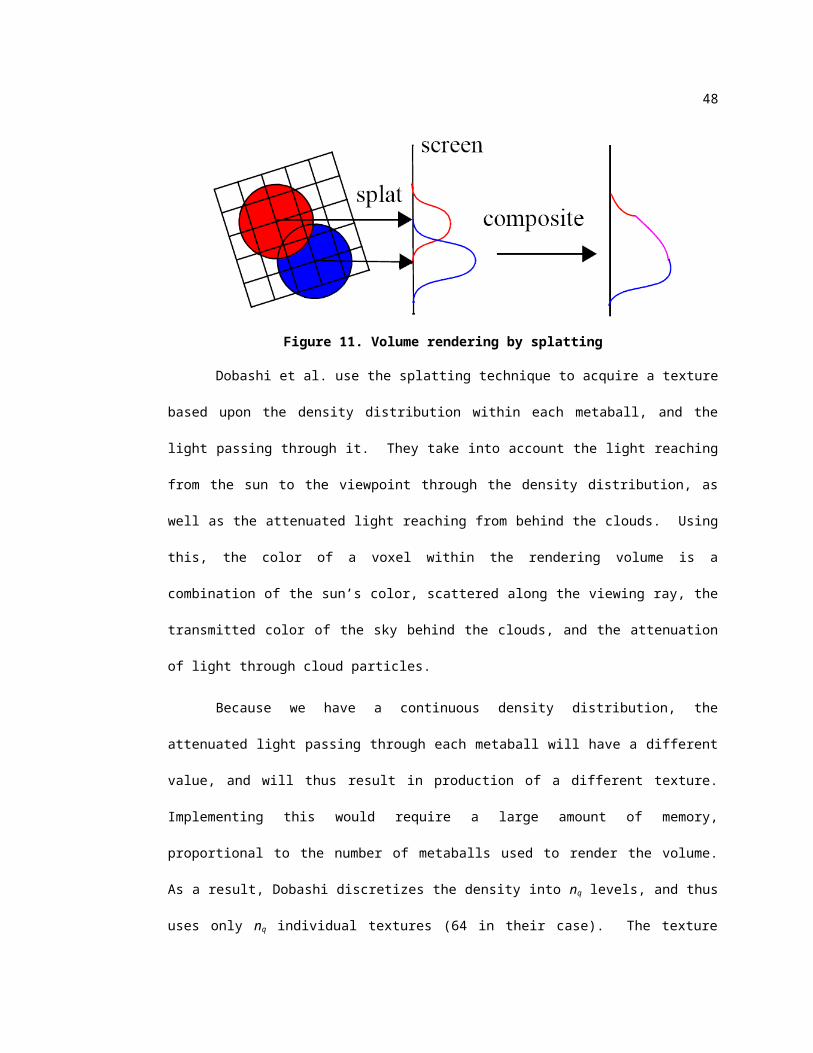
48

CHAPTER VI

CONCLUSIONS

In this project, we have implemented a parameterized, user-controllable graphical user

interface for simulating clouds in real-time. Cloud structures are simulated in a three-dimensional

volume utilizing a cellular automaton, and rendered with OpenGL. The simulation produces visually

convincing cloud-like structures based upon a set of simple transition rules which model actual cloud

growth and extinction. Wind is simulated by moving the ellipsoids which control cloud formation

probabilities based upon a set of wind equations, providing dynamic cloud movement as the simulation

progresses. By incorporating actual images of clouds as textures for rendering, we add further realism

to the cloud structure without adding more computation time to the simulation.

Several areas of improvement remain open for further investigation. First, our rendering

method includes all active voxels in the cellular automaton, and does not perform any culling of non-

visible voxels. This greatly decreases performance of the rendering as potentially millions of pieces of

geometry are rendered that have no effect on the scene. Also, our simulation rendering does not

perform any true lighting calculations, and thus the clouds end up with a somewhat flat appearance,

particularly in areas where many voxels with high density values lie atop each other, and are blended

together. Dobashi et al. included lighting calculations in their rendering, which added depth to the

scene, giving the clouds a more realistic appearance. Due to differences in how the clouds are

rendered, this approach does not lend itself easily to our rendering method. Instead, we could

potentially use OpenGL lighting directly to accomplish this. Finally, the billboards utilized for

rendering are implemented in such a way that their orientation calculations are performed on the CPU.

This is rather slow, and also takes processing time away from other jobs that are performed on the

CPU, such as the simulation itself. To alleviate this, the billboarding calculations could potentially be

performed on the graphics card’s GPU via a vertex shading program, which would allow the CPU to

be utilized for other calculations.

49

BIBLIOGRAPHY

[1] Blinn, J. F. 1982. Light reflection functions for simulation of clouds and dusty surfaces. SIGGRAPH Comput. Graph. 16, 3 (Jul. 1982), 21-29. DOI= http://doi.acm.org/10.1145/800064.801255

[2] Botsch, M., Hornung, A., Zwicker, M., Kobbelt, L. High-quality surface splatting on today's GPUs. In Proceedings Eurographics/IEEE VGTC Symposium Point-Based Graphics, vol. 0, no. 0, pp. 17-141, 2005. DOI= http://doi.ieeecomputersociety.org/10.1109/PBG.2005.194059

[3] Botsch, M. and Kobbelt, L. 2003. High-Quality Point-Based Rendering on Modern GPUs. In Proceedings of the 11th Pacific Conference on Computer Graphics and Applications (October 08 - 10, 2003). PG. IEEE Computer Society, Washington, DC, 335. DOI= http://doi.ieeecomputersociety.org/10.1109/PCCGA.2003.1238275

[4] Brickman, N., Olsen, D., Smith, G. Shapes in the Clouds: Interactive, Artist-Guided, Cloud Simulation. University of California at Santa Cruz. Computer Science Project, 2007. URL= http://www.soe.ucsc.edu/classes/cmps262/Winter07/projects/clouds/finaldraft.pdf

[5] Calidonna, C. R., Napoli, C. D., Giordano, M., Furnari, M. M., and Gregorio, S. D. 2001. A network of cellular automata for a landslide simulation. In Proceedings of the 15th international Conference on Supercomputing (Sorrento, Italy). ICS '01. ACM, New York, NY, 419-426. DOI= http://doi.acm.org/10.1145/377792.377900

[6] Cloud Condensation Nuclei. Wikipedia. Online at http://en.wikipedia.org/wiki/Cloud_condensation_nuclei.

[7] Deusen, O., Ebert, D. S., Fedkiw, R., Musgrave, F. K., Prusinkiewicz, P., Roble, D., Stam, J., and Tessendorf, J. 2004. The elements of nature: interactive and realistic techniques. In ACM SIGGRAPH 2004 Course Notes (Los Angeles, CA, August 08 - 12, 2004). SIGGRAPH '04. ACM, New York, NY, 32. DOI= http://doi.acm.org/10.1145/1103900.1103932

[8] Dobashi, Y., Nishita, T., Yamashita, H., and Okita, T. 1998. Modeling of Clouds from Satellite Images using Metaballs. In Proceedings of the 6th Pacific Conference on Computer Graphics and Applications (October 26 - 29, 1998). PG. IEEE Computer Society, Washington, DC, 53. DOI= http://doi.ieeecomputersociety.org/10.1109/PCCGA.1998.731998

[9] Dobashi, Y., Kaneda, K., Yamashita, H., Okita, T., and Nishita, T. 2000. A simple, efficient method for realistic animation of clouds. In Proceedings of the 27th Annual Conference on Computer Graphics and interactive Techniques International Conference on Computer Graphics and Interactive Techniques. ACM Press/Addison-Wesley Publishing Co., New York, NY, 19-28. DOI= http://doi.acm.org/10.1145/344779.344795

[10] Dobashi, Y., Nishita, T., Okita, T. 1998. Animation of Clouds Using Cellular Automaton. In Proceedings of Computer Graphics and Imaging ’98, 251-256.

[11] Dorsey, J., Rushmeier, H., and Sillion, F. 2008. Advanced material appearance modeling. In ACM SIGGRAPH 2008 Classes(Los Angeles, California, August 11 - 15, 2008). SIGGRAPH '08. ACM, New York, NY, 1-145. DOI= http://doi.acm.org/10.1145/1401132.1401140

50

[12] Fedkiw, R., Stam, J., and Jensen, H. W. 2001. Visual simulation of smoke. In Proceedings of the 28th Annual Conference on Computer Graphics and interactive Techniques SIGGRAPH '01. ACM, New York, NY, 15-22. DOI= http://doi.acm.org/10.1145/383259.383260

[13] Foster, N. and Metaxas, D. 1997. Modeling the motion of a hot, turbulent gas. In Proceedings of the 24th Annual Conference on Computer Graphics and interactive Techniques International Conference on Computer Graphics and Interactive Techniques. ACM Press/Addison-Wesley Publishing Co., New York, NY, 181-188. DOI= http://doi.acm.org/10.1145/258734.258838

[14] Gardner, G. Y. 1985. Visual simulation of clouds. SIGGRAPH Comput. Graph. 19, 3 (Jul. 1985), 297-304. DOI= http://doi.acm.org/10.1145/325334.325248

[15] Griebel, M., Dornseifer, T., and Neunhoeffer, T. 1998 Numerical Simulation in Fluid Dynamics: a Practical Introduction. Society for Industrial and Applied Mathematics.

[16] Harris, M. J., Coombe, G., Scheuermann, T., and Lastra, A. 2002. Physically-based visual simulation on graphics hardware. In Proceedings of the ACM SIGGRAPH/EUROGRAPHICS Conference on Graphics Hardware (Saarbrucken, Germany, September 01 - 02, 2002). SIGGRAPH/EUROGRAPHICS Conference On Graphics Hardware. Eurographics Association, Aire-la-Ville, Switzerland, 109-118.

[17] Harris, M. J. 2005. Real-time cloud simulation and rendering. In ACM SIGGRAPH 2005 Courses (Los Angeles, California, July 31 - August 04, 2005). J. Fujii, Ed. SIGGRAPH '05. ACM, New York, NY, 222. DOI= http://doi.acm.org/10.1145/1198555.1198792

[18] Harris, M. J., Baxter, W. V., Scheuermann, T., and Lastra, A. 2003. Simulation of cloud dynamics on graphics hardware. In Proceedings of the ACM SIGGRAPH/EUROGRAPHICS Conference on Graphics Hardware (San Diego, California, July 26 - 27, 2003). SIGGRAPH/EUROGRAPHICS Conference On Graphics Hardware. Eurographics Association, Aire-la-Ville, Switzerland, 92-101.

[19] Hawkins, T., Einarsson, P., and Debevec, P. 2005. Acquisition of time-varying participating media. In ACM SIGGRAPH 2005 Papers (Los Angeles, California, July 31 - August 04, 2005). J. Marks, Ed. SIGGRAPH '05. ACM, New York, NY, 812-815. DOI= http://doi.acm.org/10.1145/1186822.1073266

[20] Hu, X., Muzy, A., and Ntaimo, L. 2005. A hybrid agent-cellular space modeling approach for fire spread and suppression simulation. In Proceedings of the 37th Conference on Winter Simulation (Orlando, Florida, December 04 - 07, 2005). Winter Simulation Conference. Winter Simulation Conference, 248-255.

[21] Iben, H. N. and O'Brien, J. F. 2006. Generating surface crack patterns. In Proceedings of the 2006 ACM Siggraph/Eurographics Symposium on Computer Animation (Vienna, Austria, September 02 - 04, 2006). Symposium on Computer Animation. Eurographics Association, Aire-la-Ville, Switzerland, 177-185.

[22] Kajiya, J. T. and Von Herzen, B. P. 1984. Ray tracing volume densities. In Proceedings of the 11th Annual Conference on Computer Graphics and interactive Techniques H. Christiansen, Ed. SIGGRAPH '84. ACM, New York, NY, 165-174. DOI= http://doi.acm.org/10.1145/800031.808594

[23] Kaufman, A., Mueller, K., Johnson, C. (ed), Hansen, C. (ed). Overview of Volume Rendering. In The Visualization Handbook. Elsevier Butterworth-Heinemann, Burlington, MA 2005.

51

[24] Liao, H., Chuang, J., and Lin, C. 2004. Efficient rendering of dynamic clouds. In Proceedings of the 2004 ACM SIGGRAPH international Conference on Virtual Reality Continuum and Its Applications in industry (Singapore, June 16 - 18, 2004). VRCAI '04. ACM, New York, NY, 19-25. DOI= http://doi.acm.org/10.1145/1044588.1044591

[25] Miyazaki, R., Yoshida, S., Nishita, T., and Dobashi, Y. 2001. A Method for Modeling Clouds Based on Atmospheric Fluid Dynamics. In Proceedings of the 9th Pacific Conference on Computer Graphics and Applications (October 16 - 18, 2001). PG. IEEE Computer Society, Washington, DC, 363. DOI= http://doi.ieeecomputersociety.org/10.1109/PCCGA.2001.962893

[26] Mueller, K., Shareef, N., Jian Huang, Crawfis, R. High-quality splatting on rectilinear grids with efficient culling of occluded voxels. In IEEE Trans. on Visualization and Computer Graphics, Vol. 5, No 2, 1999.

[27] Nagel, K., Raschke, E. Self-Organizing Criticality in Cloud Formation. Physica A, 182, 1992, pp. 519-531.

[28] Neyret, F. Qualitative simulation of convective cloud formation and evolution. In Eurographics Workshop on Animation and Simulation '97, September 1997.

[29] Nishita, T. and Dobashi, Y. 1999. Modeling and Rendering Methods of Clouds. In Proceedings of the 7th Pacific Conference on Computer Graphics and Applications (October 05 - 07, 1999). PG. IEEE Computer Society, Washington, DC, 218. DOI= http://doi.ieeecomputersociety.org/10.1109/PCCGA.1999.803365

[30] Nishita, T., Dobashi, Y. Modeling and rendering of various natural phenomena consisting of particles. In Computer Graphics International 2001. Proceedings , vol., no., pp.149-156, 2001. DOI= http://doi.ieeecomputersociety.org/10.1109/CGI.2001.934669

[31] Nishita, T., Dobashi, Y., and Nakamae, E. 1996. Display of clouds taking into account multiple anisotropic scattering and sky light. In Proceedings of the 23rd Annual Conference on Computer Graphics and interactive Techniques SIGGRAPH '96. ACM, New York, NY, 379-386. DOI= http://doi.acm.org/10.1145/237170.237277

[32] Overby, D., Melek, Z., and Keyser, J. 2002. Interactive Physically-Based Cloud Simulation. In Proceedings of the 10th Pacific Conference on Computer Graphics and Applications (October 09 - 11, 2002). PG. IEEE Computer Society, Washington, DC, 469. DOI= http://doi.ieeecomputersociety.org/10.1109/PCCGA.2002.1167904

[33] Perlin, K. and Hoffert, E. M. 1989. Hypertexture. In Proceedings of the 16th Annual Conference on Computer Graphics and interactive Techniques SIGGRAPH '89. ACM, New York, NY, 253-262. DOI= http://doi.acm.org/10.1145/74333.74359

[34] Pallister, K., Deloura, M. (ed). 2001. Generating Procedural Clouds Using 3D Hardware. In Game Programming Gems 2. Charles River Media, Inc, Rockland, MA.

[35] Roden, T. and Parberry, I. 2005. Clouds and stars: efficient real-time procedural sky rendering using 3D hardware. In Proceedings of the 2005 ACM SIGCHI international Conference on Advances in Computer Entertainment Technology (Valencia, Spain, June 15 - 17, 2005). ACE '05, vol. 265. ACM, New York, NY, 434-437. DOI= http://doi.acm.org/10.1145/1178477.1178574

[36] Sarkar, P. 2000. A brief history of cellular automata. ACM Comput. Surv. 32, 1 (Mar. 2000), 80-107. DOI= http://doi.acm.org/10.1145/349194.349202

52

[37] Schpok, J., Simons, J., Ebert, D. S., and Hansen, C. 2003. A real-time cloud modeling, rendering, and animation system. In Proceedings of the 2003 ACM Siggraph/Eurographics Symposium on Computer Animation (San Diego, California, July 26 - 27, 2003). Symposium on Computer Animation. Eurographics Association, Aire-la-Ville, Switzerland, 160-166.

[38] Stam, J. 1999. Stable fluids. In Proceedings of the 26th Annual Conference on Computer Graphics and interactive Techniques International Conference on Computer Graphics and Interactive Techniques. ACM Press/Addison-Wesley Publishing Co., New York, NY, 121-128. DOI= http://doi.acm.org/10.1145/311535.311548

[39] Wallen, R. N. 1992. Introduction to Physical Geography. Wm. C. Brown Publishers, Dubuque, IA.

[40] Wei, X., Li, W., Mueller, K., and Kaufman, A. 2002. Simulating fire with texture splats. In Proceedings of the Conference on Visualization '02 (Boston, Massachusetts, October 27 - November 01, 2002). VISUALIZATION. IEEE Computer Society, Washington, DC, 227-235.

[41] Wolfram, S. 2002. A New Kind of Science. Wolfram Media, Inc, Champaign, IL.

[42] Wolfram, S. Cellular Automaton. From Wolfram Math World. URL= http://mathworld.wolfram.com/CellularAutomaton.html

[43] Wyvill, G. and Trotman, A. 1990. Ray-tracing soft objects. In Proceedings of the Eighth international Conference of the Computer Graphics Society on CG international '90: Computer Graphics Around the World (Institute of Systems Science, Singapore). T. Chua and T. L. Kunii, Eds. Springer-Verlag New York, New York, NY, 469-476.

[44] Zwicker, M., Pfister, H., van Baar, J., and Gross, M. 2001. Surface splatting. In Proceedings of the 28th Annual Conference on Computer Graphics and interactive Techniques SIGGRAPH '01. ACM, New York, NY, 371-378. DOI= http://doi.acm.org/10.1145/383259.383300

[45] Zwicker, M., Räsänen, J., Botsch, M., Dachsbacher, C., and Pauly, M. 2004. Perspective accurate splatting. In Proceedings of Graphics interface 2004 (London, Ontario, Canada, May 17 - 19, 2004). ACM International Conference Proceeding Series, vol. 62. Canadian Human-Computer Communications Society, School of Computer Science, University of Waterloo, Waterloo, Ontario, 247-254.