Dynamic Bandwidth Allocation for Multimedia Traffic withRate Guarantee and Fair Access in WCDMA Systems ∗

Chih-Min Chao1, Yu-Chee Tseng2, and Li-Chun Wang3

1 Department of Information Management

Tamkang University, 25165, Taiwan

Tel: +886-3-2652914, Fax: +886-3-2652999

Email: cmchao@axp1.csie.ncu.edu.tw (corresponding author)2 Department of Computer Science and Information Engineering

National Chiao-Tung University, 30050, Taiwan

Tel: +886-3-5712121 ext. 54782, Fax: +886-3-5724176

Email: yctseng@csie.nctu.edu.tw3 Department of Communication Engineering

National Chiao-Tung University, 30050, Taiwan

Tel: +886-3-5712121 ext. 54511, Fax: +886-3-5710116

Email: lichun@mail.nctu.edu.tw

Abstract

Packet scheduling in a WCDMA system poses a new challenge due to its nature

of variable bit rates and location-dependent, time-varying channel conditions. In

this work, three new downlink scheduling algorithms for a WCDMA base station

are proposed to support multimedia transmissions. Using a credit management

and a compensation mechanism, our algorithms provide rate guarantee and fair

access to mobile terminals. In particular, we propose to allow a user to simultane-

ously use multiple OVSF codes in a time-sharing manner, which we call a multi-

code, shared model. Using multiple codes allows us to compensate those users

suffering from bad communication quality or even errors. The proposed schemes

can tolerate a multi-state link condition (compared to the typically assumed two-

state, or good-or-bad, link condition) by adjusting the number of OVSF codes

∗Y. C. Tseng’s research is co-sponsored by the MOE Program for Promoting Academic Excellence ofUniversities under grant number 89-E-FA04-1-4, by NSC of Taiwan under grant numbers NSC92-2213-E009-076 and NSC92-2219-E009-013, by the Institute for Information Industry and MOEA, R.O.C,under the Handheld Device Embedded System Software Technology Development Project, by the Leeand MTI Center of NCTU, and by Computer and Communications Research Labs., ITRI, Taiwan.

1

and the spreading factor of each code. Simulation results show that the proposed

schemes do achieve higher bandwidth utilization while keeping transmission delay

low.

Keywords: Mobile computing, OVSF, Personal communication services, WCDMA,

Wireless communication, 3G.

1 Introduction

Supporting multimedia applications with quality of service (QoS) requirements is one of

the ultimate goals in next-generation wireless systems. The current second-generation

(2G) systems, such as IS-95 (CDMA) and GSM (TDMA), are circuit-switched, fixed-

rate, and voice-traffic-oriented, and thus not appropriate to support multimedia services.

The third-generation (3G) wireless standards [1, 2, 12] will be based on the WCDMA

technologies and can flexibly support mixed- and variable-rate services. Two transmis-

sion schemes are proposed in the 3G wireless standard: multicode-CDMA (MC-CDMA)

and Orthogonal Variable Spreading Factor CDMA (OVSF-CDMA). In MC-CDMA,

multiple Orthogonal Constant Spreading Factor (OCSF) codes can be assigned to a

user [10, 13]. The maximum data rate a user can receive depends on the number of

transceivers in the device. In OVSF-CDMA, a single OVSF code can provide a data

rate that is several times than that of an OCSF code, depending on its spreading factor

[2].

In CDMA systems, multiple connections are allowed to receive packets simultane-

ously. This is opposite to TDMA systems where only one connection can be active at

any moment. Thus, the scheduling problem for WCDMA systems is harder than that for

TDMA systems. It can neither be solved directly by wireline scheduling disciplines, such

as WFQ [19], virtual clock [27], and EDD [15], since they do not consider the variability

of wireless connections, nor be solved by wireless scheduling strategies, such as IWFQ

[16], CIF-Q [18], and SBFA [21], since they only consider a single-server, two-state link

2

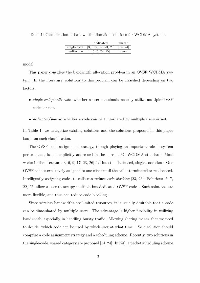
Table 1: Classification of bandwidth allocation solutions for WCDMA systems.

dedicated sharedsingle-code [3, 6, 9, 17, 23, 26] [14, 24]multi-code [5, 7, 22, 25] ours

model.

This paper considers the bandwidth allocation problem in an OVSF WCDMA sys-

tem. In the literature, solutions to this problem can be classified depending on two

factors:

• single-code/multi-code: whether a user can simultaneously utilize multiple OVSF

codes or not.

• dedicated/shared: whether a code can be time-shared by multiple users or not.

In Table 1, we categorize existing solutions and the solutions proposed in this paper

based on such classification.

The OVSF code assignment strategy, though playing an important role in system

performance, is not explicitly addressed in the current 3G WCDMA standard. Most

works in the literature [3, 6, 9, 17, 23, 26] fall into the dedicated, single-code class. One

OVSF code is exclusively assigned to one client until the call is terminated or reallocated.

Intelligently assigning codes to calls can reduce code blocking [23, 26]. Solutions [5, 7,

22, 25] allow a user to occupy multiple but dedicated OVSF codes. Such solutions are

more flexible, and thus can reduce code blocking.

Since wireless bandwidths are limited resources, it is usually desirable that a code

can be time-shared by multiple users. The advantage is higher flexibility in utilizing

bandwidth, especially in handling bursty traffic. Allowing sharing means that we need

to decide “which code can be used by which user at what time.” So a solution should

comprise a code assignment strategy and a scheduling scheme. Recently, two solutions in

the single-code, shared category are proposed [14, 24]. In [24], a packet scheduling scheme

3

is provided but the code allocation issue is not addressed. A credit-based scheduling

scheme is proposed in [14]. However, this scheme does not consider channel quality,

which may impact the selected spreading factor. A more comprehensive review is in

Section 1.1.

In this paper, we propose three new credit-based bandwidth allocation schemes that

allow a user to utilize multiple time-shared codes. This is more flexible than what

proposed in existing works. With our credit management mechanism and the compen-

sation mechanism provided by additional codes, the schemes can provide fair access and

data rate guarantee. Using multiple OVSF codes has two purposes. First, it is for

compensation purpose when a terminal encounters errors. Second, it can adapt to a

multi-link-state environment, in the sense that a higher spreading factor can be used

when the link quality is bad; however, the user can still enjoy the guaranteed bandwidth

supported by multiple codes. Simulation results show that the proposed schemes can

achieve higher bandwidth utilization and keep average delay low.

The rest of this paper is organized as follows. In Section 2, we introduce the sys-

tem model. Section 3 presents the proposed dynamic bandwidth allocation algorithms.

Performance evaluations are in Section 4. Concluding remarks are given in Section 5.

1.1 Related Works

In the dedicated, single-code class, reference [23] shows that significant improvement can

be obtained by using a leftmost-first or a crowded-first strategy, compared to a random

assignment. When a code tree is used for long time, it is possible that the tree may

become too fragmented, due to calls arriving and leaving the system. Code replacement

can be conducted to improve bandwidth utilization. The dynamic code assignment

(DCA) scheme [17] is designed for this purpose. In this case, code assignment is semi-

dedicated, in the sense that a call can be moved to a different code when relocation is

conducted.

4

Allowing a user to occupy multiple dedicated codes provides more adaptability. The

works in [7, 22] address the relationship between a requested data rate and the number of

codes to be assigned to the request. However, the placement of codes in the OVSF code

tree is left unspecified. A multi-code scheduling scheme to be run on the base station

is proposed in [25], where fair scheduling for users to share the resources is addressed.

Again, the important code placement issue is left unaddressed. In [5], both the code

placement and replacement issues are addressed for such an environment.

The scheme proposed in [14] is a member in the single-code, shared class. Initially,

each user is assigned a leaf code (of the lowest rate). However, the scheduling algorithm

would allow a user to utilize any ancestor code of its assigned code. In each time frame,

the algorithm will repeatedly pick the user with the highest credit, say A, and try to

move A’s code one level up from its current stand if A still has backlog packets to be

sent. This increase also means sacrificing other users’ assigned, but unused, codes. That

is, the latter will be inhibited from transmission in this round. The process is repeated

until all capacities in the code tree are consumed or no packet is pending. Inhibited

users’ credits will be increased in the next frame. This scheme fails to consider the

possible higher bit error rate (BER) that is caused by using a lower spreading factor.

Depending on the channel condition, the spreading factor should not be unlimitedly

reduced. Otherwise, a lot of retransmissions may be incurred, resulting in even worse

performance. The scheme also includes an exception handling mechanism to solve the

starvation problem that may occur during scheduling.

2 System Model

In the WCDMA system [20], data transmission involves two steps. The first step is

channelization, which transforms every data bit into a code sequence. The length of

the code sequence per data bit is called the spreading factor (SF), which is typically a

power of two. The second step is scrambling, which applies a scrambling code to the

5

C1,1

C2,1

SF=1

SF=2

SF=4

SF=8

C4,2 C4,3 C4,4C4,1

C8,1 C8,5 C8,6 C8,7 C8,8C8,2 C8,3 C8,4

C2,22

1

11

1

1

1

3

0

0000

1

1

Figure 1: A code blocking scenario (busy codes are marked by gray).

spread signal. Scrambling codes are used to separate signals from different sources, while

channelization codes multiplex data to different users from the same source.

The OVSF codes are used as the channelization codes in the WCDMA system. The

possible OVSF codes can be represented by a code tree as shown in Fig. 1. Each OVSF

code is denoted as CSF,k, where SF is the spreading factor and k is the branch number,

1 ≤ k ≤ SF . The number of codes at each level is equal to the value of SF . All codes

in the same layer are orthogonal, while codes in different layers are orthogonal only if

they do not have ancestor-descendant relationship. Leaf codes have the minimum data

rate, which is denoted by 1Rb. The data rate is doubled whenever we go one level up

the tree. For example, in Fig. 1, C4,1 has rate 2Rb, and C2,1 has rate 4Rb. The resource

units in a code tree are codes. Fig. 1 shows an example where codes C4,2, C8,1, and

C8,5 are occupied by users. The remaining capacity is 4Rb. If the dedicated, single-code

model is assumed, a new call requesting a rate of 4Rb will be rejected because there is

no such code available. Such situation is called code blocking. However, the problem can

be solved if up to three codes can be used by a user under the multi-code model.

A main characteristic of wireless communications is link variability, which could be

time-dependent and location-dependent. It is time-dependent because interference can

come to hit at any time. One example frequently seen is bursty errors. The capacity

of a wireless link is location-dependent because a longer distance typically has to suffer

6

lower transmission rate. These properties necessitate the design of dynamic bandwidth

allocation mechanisms.

Since the quality of a wireless link is both time- and location-dependent, we assume

that its capacity follows a multi-state model. Specifically, a wireless link’s symbol error

rate is inversely proportional to its received signal strength, which is given by Eb

N0=

SNR×SF , where Eb is the energy per bit, N0 is two times the power spectral density of

additive white Gaussian noise, SNR is the signal-to-noise ratio, and SF is the spreading

factor. To achieve a target Eb/N0, one can either increase SNR through power control

or increase the spreading factor SF . When the transmission power is up to a limit,

increasing SF is the only way to reduce bit error rate. In this work, we assume that

there exists a target BER for all users. As a result, at any moment, there is always

a maximum data rate (and thus minimum spreading factor) for each user. In such

an environment, the scheduling problem is still an open question [4]. Most existing

scheduling strategies [8, 11, 16, 18, 21] consider a simple two-state channel model where

a channel can be either good or bad, receiving full or none capacity, respectively.

This paper considers the downlink bandwidth allocation problem for a base station.

The resource at the base station is an OVSF code tree. Each user i, when entering the

system, needs to specify its peak data rate piRb and guaranteed data rate aiRb. Both pi

and ai are powers of two and pi ≥ ai. The base station maintains a queue Qi for user

i’s packets to be delivered. So the inputs to our scheduling algorithms are pi, ai, and Qi,

for all users i = 1..n. The base station is responsible of utilizing its code tree to serve

users efficiently and fairly. According to the current 3G standard, each frame is 10 ms,

which consists of 15 slots. So in every 10 ms, we can reschedule codes for users. The

purpose of bandwidth allocation is to achieve high utilization while providing guarantee

rates for individual users.

We assume the shared, multi-code model, where a user can simultaneously use up

to Nmax codes. This model has several advantages: (1) when a user suffers severe

7

interference, we can increase the spreading factor to improve reliability but maintain

the promised data rate by using multiple codes, and (2) when a user suffers temporary

degradation, compensation can be made up to it by using multiple codes for fairness.

3 Dynamic Bandwidth Allocation Strategies

This section presents our dynamic bandwidth allocation strategies to provide QoS-

guaranteed services. Our solutions consist of three parts: code assignment, credit man-

agement, and packet scheduling.

3.1 Code Assignment Part

This part decides which codes should be assigned to each user to satisfy his/her demand.

We assume that there is an admission control mechanism such that a user is accepted

only if the sum of guaranteed data rates over all users does not exceed the capacity of

the code tree. For each code k in the code tree, the base station maintains a variable

(SCk) (read as shared count) to keep track of the number of users who are currently

sharing k, either partially or completely. Specifically, a user is said to share code k if the

user is using code k, a descendant code of k, or an ancestor code of k. For example, in

Fig. 1, the number in each node is the corresponding code’s shared count. It is easy to

maintain the shared counts. Whenever a code k is allocated to a user, the shared counts

of k and k’s ancestor and descendant codes are all increased by one. These counts are

decreased by one when this user leaves.

Note that, in contrast to the code assignment in [14], which assigns a leaf code to

each user initially, we allocate codes to users according to their maximal data rates.

During transmission, a user can use any of the descendent codes of the initially assigned

one, which is compatible to the 3gpp standard [1].

8

3.1.1 Scheme 1: Multiple Fixed Codes

In this scheme, we allocate Nmax fixed codes, each of rate pi ·Rb, to user i. Under normal

situations, only one code is sufficient. The additional codes can be used for interference

reduction or bandwidth compensation. This will be further elaborated in Section 3.3.

Given user i’s request, the scheme sequentially picks Nmax codes. To allocate each

code, the following rules are applied:

1. Scan all codes in the code tree with rate piRb. Pick the one(s) with the least shared

count. If there is only one candidate, assign this code to user i. Otherwise, go to

step 2.

2. If the shared counts of these candidate codes are 0s, we follow the crowded-first rule

to do the allocation. Specifically, if x and y are two codes such that SCx = SCy =

0, we compare x’s and y’s parent codes. The one with a larger SC is selected.

If they tie again, we further compare their parents. This is repeated until the tie

breaks. One special case is that x’s and y’s parents could be the same code. If so,

we simply select the one on the left-hand side.

3. If the shared counts of the candidate codes are non-zero, we follow the fairness

rule. Specifically, if x and y are two codes such that SCx = SCy 6= 0, we compare

x’s and y’s parent codes similar to the recursive procedure in step 2. However, we

select the code with a smaller shared count, instead of a larger one.

Intuitively, when there are still free codes, we try to place users’ requests in the code

tree as compact as possible (this is what suggested in [23]). Otherwise, some degree of

sharing among users is necessary, and we try to assign codes as fairly as possible.

Take the scenario in Fig. 2(a) as an example. Suppose Nmax = 2 and a new user

requests for a 2Rb rate. After searching for all 2Rb codes, we find that C8,2, C8,5, C8,6,

and C8,8 all have zero shared counts. So we further compare their ancestors, C4,1, C4,3,

9

C4,1 C4,1C4,3 C4,2C4,4 C4,4

C2,1C2,1C2,2

C2,2

C8,2 C8,4 C8,6C8,5 C8,8C8,1

(a)

C8,3

C16,1

C8,3 C8,4C8,7 C8,7 C8,8

(b)

6

4

1

1 1 1 11 1 11

1

2

2

2 2 2 2 2

244

5

11

4

11

1111

1

1

1 1 1 1111

1

11111

2 0

0 000

0

6

00 0000 0

2

2

Figure 2: A code assignment example when the code tree has (a) free 2Rb codes and (b)no free 2Rb code. The number in each node is its shared count.

and C4,4. Among them, C4,1 and C4,4, which have the same shared counts of two, tie

again. After going one level up, we see that C2,1 has a larger shared count than C2,2. So

C8,2 is allocated to the user. The same procedure is applied to allocate the second code.

This time C8,8 will be picked. Another example where the code tree is fully occupied is

shown in Fig. 2(b). Again, assuming the same situation, step 1 will pick C8,3, C8,4, C8,7,

and C8,8, all of which have the same shared count = 1. After going one level up, we see

that C4,2 has a smaller shared count. Since C8,3 and C8,4 tie, following the leftmost-first

rule, we will select C8,3. To assign the second code, we see that C8,4, C8,7, and C8,8 all

have the same least SC value. Their ancestors, C4,2 and C4,4, tie again with the same

SC value of two. Another tie is found when coming to codes C2,1 and C2,2. Since C2,1

and C2,2 have the same ancestor, the leftmost candidate, C8,4, will be assigned to the

user.

3.1.2 Scheme 2: Single Fixed Code with Multiple Dynamic Codes

This scheme only assigns one fixed code to each user. The other Nmax − 1 codes are

all assigned in a dynamic manner. Specifically, the OVSF code tree is partitioned into

two areas: partially shared area on the left and fully shared area on the right (how to

select a good partition point will be evaluated in Section 4). Given a user requesting a

rate piRb, it is assigned a code of rate piRb in the partially shared area. The assignment

follows the same rule in the previous scheme except that only the partially shared area

10

is assignable. The remaining Nmax − 1 codes will be assigned to the fully shared area,

but the assignment will not be done in this stage and will be decided at the scheduling

stage.

3.1.3 Scheme 3: No Fixed Codes

In contrast to the previous schemes, this scheme does not assign any fixed code to users.

All Nmax codes will be allocated dynamically at the scheduling stage. This scheme

provides the maximal flexibility (alternatively, one can consider the whole OVSF code

tree as a fully shared area in Scheme 2).

3.1.4 Remark on Code Notification

The codes used in our schemes can be directly mapped to the transport channels in 3gpp.

To schedule users, the Forward Access Channel (FACH) can be used to notify them their

transmission data rates as well as codes. An additional ID field is needed in the header

to distinguish users (we will analyze the signaling overhead in Section 3.4). In schemes 1

and 3, all codes allocated to a user can be mapped to the Dedicated Transport Channel

(DCH). In scheme 2, the single fixed code can be mapped to DCH, while the remaining

dynamic codes to Downlink Share Channel (DSCH). According to 3gpp, a DSCH is

always associated with a DCH, which provides necessary signaling for the DSCH.

3.2 Credit Management Part

In the above part, we already assigned each user multiple codes which exceed the user’s

guaranteed data rate. These codes are not necessarily always used by the user. We

employ a credit management mechanism to dynamically allocate bandwidths to users.

The base station maintains a credit Ci for each user i. Initially, Ci = 0. After every

10 ms, ai credits, i.e., user i’s guaranteed rate, are granted to user i and added to Ci.

However, for every code of rate 2kRb that is consumed by user i, 2k credits are paid by

decreasing 2k from Ci. Hence, as a user’s perceived data rate is below its guaranteed

11

rate, its credits can be accumulated for later use. The value of Ci can also be negative,

if the user is over-served (which happens, for example, if other users under-use their

capacities due to poor channel condition). Long-term fairness and rate guarantee are

provided if the base station honors all users’ credits.

Care should be taken if a user’s perceived data rate is below his/her request rate

for long time, due to reasons such as poor channel condition, sudden congestion, or

simply low data arrival rate. In this case, a lot of credits may be accumulated for the

user. Later on, if a large amount of traffic arrives for the user, the user may take up a

lot of bandwidth, thus blocking the opportunity of other users. This is alright if only

long-term rate guarantee is required, but it does cause a problem viewed for a short

term. Short-term fairness is not guaranteed if we allow a user to accumulate credits

unlimitedly. To resolve this problem, we propose to maintain a credit limit Li for each

user i such that Ci ≤ Li is always true. The value of Li can be negotiated with the base

station in a per-user basis when the connection was first established according to the

user’s priorities, degree of burstiness, or even the system loading.

Note that we do not distinguish the situation that a user has lower traffic than

expected from that it suffers from bad channel condition. In both situations, it can

accumulate credits. An alternative is to apply the credit limit only in the former case

[14]. However, we believe that it is more reasonable to apply the limit to both cases

because wireless channels may suffers from burst errors more frequently.

3.3 Packet Scheduling Part

The scheduling algorithm is executed once every 10 ms (frame length). It examines all

users with backlog data at the base station, and determines which users to be served by

which codes. The goal is to provide a fair and rate-guaranteed service to each user.

12

3.3.1 Scheduling for Scheme 1 (Multiple Fixed Codes)

To facilitate the scheduling scheme, we introduce the term normalized credit of user i,

which is defined to be the ratio Ci/ai. The normalized credit represents the amount of

services a user i should receive relative to his/her guaranteed rate ai. A user with the

greatest normalized credit, instead of credit, should be scheduled first. The scheduling

algorithm for scheme 1 has six steps.

• STEP 1. Sort all users according to their normalized credits.

• STEP 2. Pick the user, say i, with the greatest normalized credit such that user

i has backlog packets and at least one of user i’s codes is free. If there is no such

user, the procedure terminates.

• STEP 3. Let Mi be the maximum bit rate for user i such that the BER is satisfied

(this can be obtained by monitoring the channel condition).

• STEP 4. Let Ti = min{Mi, pi}, which represents the feasible transmission rate

considering user i’s channel quality. We search all free codes of user i. If there

exists at least one free code, we allocate the leftmost one for user i. Otherwise,

we go one level down by searching all descendant codes (of rate Ti

2Rb) of user i’s

codes. If there exist at least one free code, we allocate the leftmost one for user

i. Otherwise, we repeat the same procedure and search the descendant codes of

rates Ti

4, Ri

8, · · · , etc.

• STEP 5. For the code allocated in STEP 4, we decrease user i’s credit Ci by the

corresponding amount. Then, user i is put in to the sorted list.

• STEP 6. Go back to STEP 2.

Take Fig. 3 as an example. Suppose that user i has the greatest normalized credits

and C8,1, C8,2, and C8,3 are user i’s codes. When user i is selected for the first time, only

13

C4,1 C4,3 C4,4

C2,1 C2,2

C8,2 C8,4 C8,6C8,5 C8,8C8,1

C16,1 C16,2 C16,16

C8,3 C8,7

4

Figure 3: A scheduling example. Codes marked by gray are occupied.

C8,2 is free. So C8,2 is allocated to serve user i in the next frame and two credits are

subtracted from Ci. If user i is selected for the second time, C16,2 will be allocated to it.

3.3.2 Scheduling for Scheme 2 (Single Fixed Codes with Multiple DynamicCodes)

The scheduling algorithm is similar to the previous case. The difference lies on how a

user’s codes are used. All steps are the same as the previous case, except step 4, which

is described below.

• STEP 4′. If this is the first time user i is selected in this frame, go to (a). Otherwise,

go to (b).

– (a) Let Ti = min{Mi, pi}. We search the single fixed code of user i. We

allocate it to user i if it is free. Otherwise, we go one level down by searching

all descendant codes (of rate Ti

2Rb) of user i’s code. If there exists at least

one free code, we allocate the leftmost one to user i. Otherwise, we repeat

the same procedure and search the descendant codes of rates Ti

4, Ti

8, · · · , etc.

If we can’t find a free code, user i is skipped for further scheduling in the

current time frame.

– (b) Allocate a free code at the fully shared area (this is similar to case (a)

but we have more freedom because any free code can be allocated).

14

Again, take Fig. 3 as an example. Let the quarter of the code tree on the right-hand

side be the fully shared area. Suppose that user i has the highest normalized credit and

C8,1 is his/her initial code. The scheduling algorithm will allocate C16,2 to user i’s in

the first round. If user i is selected again for next two rounds, C16,15 and C16,16 in the

fully shared area will be allocated to it. On the contrary, if C8,3 is user i’s initial code,

it can’t be scheduled in the current frame because C8,3 is already occupied by another

user.

3.3.3 Scheduling for Scheme 3 (No Fixed Codes)

The algorithm is similar to the previous two schemes. It follows scheme 1, except the

following modifications:

• STEP 2′′. The same as STEP 2 except that we only need to make sure that user

i has not exhausted its Nmax codes.

• STEP 4′′. The same as STEP 4 except that any free space in the code tree can be

used by user i.

3.4 Time Complexity and Signaling Overhead Analysis

Next, we analyze the time complexity of our schemes. Consider the code assignment

part. There are SF codes in the code tree with a spreading factor of SF . So the cost

is O(SF ) to search for such a code. For the fixed code assignment part of scheme 1, we

may need to compare the shared counts of candidate codes’ ancestors. Each time when

we go one level up the code tree, the number of ancestors reduces by half. It is easy to

see that the cost to allocate a code with a specific SF is SF + SF2

+ · · · + 1 = O(SF ).

Thus, to assign Nmax codes, the searching cost is O(Nmax × SF ) = O(SF ) because

Nmax is a constant. The time complexity for the fixed code assignment part of scheme

2 is similar to that of scheme 1, except that the searching domain is restricted to the

partially shared area. So the time complexity is the same.

15

For the credit assignment part, it is easy to see that the time complexity is O(n)

for all three schemes, where N is the number of users currently in the system. For

the packet scheduling part, all three schemes need to sort all users, giving a cost of

O(n log n). The STEP 4 of scheme 1 may spend 1 + 2 + · · · + SFmax

SF= O(SFmax

SF) time

to find a free code, where SFmax is the maximum allowable SF . So the total searching

cost is O(n′× SFmax

SF), where n′ is the actual number of transmissions that are scheduled

in this time frame. STEP 5 takes O(n) to put the scheduled user back to the sorted

list. For scheme 2, the searching cost of STEP 4’(a) is O(np × SFmax

SF), where np is the

number of scheduled transmissions in the partially shared area. In STEP 4’(b), each

code assignment takes O(SF ) time, so the total cost is O(nf × SF ), where nf is the

number of scheduled transmissions in the fully shared area. Similarly, for scheme 3, the

searching cost of STEP 4” is O(n′ × SF ).

Overall, the time complexity for scheme 1 is O(SF +n log n+n′× SFmax

SF). For scheme

2, the time complexity is O(SF + n log n + np × SFmax

SF+ nf × SF ). For scheme 3, the

time complexity is O(SF + n log n + n′ × SF ). The complexities are typically low. For

example, in our simulations, with SFmax = 256, the value of n is around 68, which should

take less than tens of microseconds to complete these calculations in modern processors.

The signaling overhead for scheme 1 is n′×dlg S1e, where S1 is the maximum number

of users that use the same code. For scheme 2, the signaling overhead is np × dlg S2e+

nf × dlg n2e, where S2 is the maximum number of users that use the same code in

the partially shared area and n2 is the number of codes in the fully shared area. The

signaling overhead for scheme 3 is n′ × dlg n3e, where n3 is the number of codes in the

code tree.

4 Performance Evaluation

We have implemented a simulator to evaluate the performance of the proposed strategies.

The max SF is set to 256. We control the call generation such that the overall guaranteed

16

traffic load falls between 10% and 90%. Three traffic models are tested [14]:

• Model I (constantly backlogged model) : Each user has queued packets all the

time. Each user’s peak transmission rate is uniformly distributed between 4Rb

and 32Rb, and guaranteed rate one fourth of the peak rate (i.e., ai = 14pi).

• Model II (highly bursty traffic model) : Calls are generated into the system with

a peak rate uniformly distributed between 4Rb and 32Rb and a guaranteed rate

equal to one fourth of the peak rate. Packet arrival of each connection follows a

2-state Markov model. A connection can transit between an idle state or an active

state. No packet is generated during the idle state, while P packets per 10 ms are

generated during the active state, where P is uniformly distributed between 2ai

and 4ai. A state transition can be made every 10 ms, with probabilities of 1/3 and

2/3 from idle to active and from active to idle, respectively.

• Model III (lowly bursty traffic model) : Calls are generated into the system with

a peak rate uniformly distributed between 2Rb and 16Rb and a guaranteed rate

equal to one half of the peak rate. Packet arrival also follows the above 2-state

Markov model, but P is uniformly distributed between ai and 2ai while state

transition probabilities are 2/3 and 1/3 from idle to active and from active to idle,

respectively.

Each transport block is set to 150 bits, which means a 1Rb code can transmit 150

bits every 10 ms. A transport block will be retransmitted if an error is detected by the

cyclic redundancy check (we assume no channel coding is applied). In schemes 1, 2, and

3, Nmax ranges from 2 to 4. In scheme 2, the first three quarters of the code tree is the

partially shared area, and the last quarter is the fully shared area.

Using the QPSK modulation, we model the symbol error probability by

PE ≈ 2Q

(√2Eb

N0

), (1)

17

0

5

10

15

20

25

30

35

40

45

50

10 20 30 40 50 60 70 80 90traffic load (%)

unsa

tisf

acto

ryitra

nsm

issi

on

(%) = 1

= 2.5= 5= 10= 25= 50

Figure 4: Unsatisfactory transmission versus traffic load at different γ for the KMSscheme [14].

where

Q(x) =

∫ ∞

x

e−y2/2

√2π

dy

and

Eb

N0

= SNR× SF.

Intuitively, the transmission rate is inversely proportional to the SF being applied. A

lower SF has a higher transmission rate but the potential penalty, according to Eq.(1),

is a higher PE. To achieve a better throughput, we should choose the smallest SF that

meets the required PE. A scheme without considering channel condition, such as [14]

(denoted by KMS below), is impractical because it may choose an improper SF and

thus suffer from severe performance degradation. In this paper, the upper bound of PE

is set to 10−5. We assume a Rayleigh fading channel, so signal power is modelled by an

exponential random variable X with mean γ, i.e., f(x) = 1γe−xγ for x ≥ 0 [20].

We first experiment on the KMS scheme on traffic model II by varying γ and eval-

uating the unsatisfactory transmission, which is defined to be the percentage of frames

that experiences a symbol error rate PE exceeding the threshold 10−5. As expected,

KMS performs highly depending on the channel condition. At low γ, a lot of packets

may experience failures. So the scheme is not channel-sensitive. To keep the failure rate

18

Figure 5: Code utilization (in curves) and effective code utilization (in bars) versustraffic load under traffic model II with (a) γ = 1 and (b) γ = 25.

low, say under 5%, γ should be maintained 25 or higher. Note that traffic load would

increase the error rate because the KMS scheme favors users with more backlogged

packets. This would aggravate error transmission.

Below, we further experiment on four aspects. Each result below is from an average

of 50 simulation runs, where each run contains at least 3000 frames.

A) Impact of Code Assignment Strategies: This experiment tests different code as-

signment strategies. We evaluate three metrics: code utilization, effective code utiliza-

tion, and average delay. Code utilization is the average capacity of the code tree that is

actually used for transmission. However, considering those transmissions experiencing

failure, effective code utilization counts only those successfully transmitted bits. In ad-

dition to the KMS scheme, we also simulate the “single-code, shared” scheme and the

“single-code, dedicated” scheme.

Fig. 5 shows the code utilization and effective code utilization at various traffic loads.

For our schemes, Nmax is set to 2. For code utilization, our scheme 3 performs the best,

which is sequentially followed by the KMS scheme, our scheme 2, our scheme 1, and then

the single-code schemes. After taking failure transmissions into account, effective code

utilization of KMS scheme reduces significantly when γ = 1. For example, when the

19

(a) (b)

0

20

40

60

80

100

120

10 20 30 40 50 60 70 80 90

traffic load (%)

aver

agei

del

ay

Single, sharedScheme 1Scheme 2Scheme 3KMS

0

20

40

60

80

100

120

140

160

10 20 30 40 50 60 70 80 90

traffic load (%)

av

era

gei

dela

y

Single, sharedScheme 1Scheme 2Scheme 3KMS

Figure 6: Average delay versus traffic load under traffic model II with (a) γ = 1 and (b)γ = 25.

code tree is 90% fully loaded, KMS’s effective utilization reduces to around 51%, while

our schemes can still maintain an effective utilization over 85%. Only when the channel

condition is extremely good (such as γ = 25), can KMS maintain high effective code

utilization. Since our schemes have considered channel condition, the code utilization

and effective code utilization are very close.

Fig. 6 shows the average delay, which is defined as the average time, measured in

time frames, a transport block is queued at the base station. With γ = 1, our scheme

3 experiences the least delay, which is subsequently followed by our scheme 2, scheme

1, single-code, shared scheme, and KMS. Our scheme 3 produces low delay since there

is no code blocking. The delays for scheme 1 and single-code, shared scheme increase

significantly when the code tree is above 80% loaded, which means the system is unstable

then. The KMS scheme makes the system unstable after traffic load is over 30%. These

results reveal that our scheme 3 and scheme 2 can accept more time-bounded services.

The delays of KMS reduces significantly when γ = 25, which is reasonable since the

channel condition is pretty good.

B) Fairness Properties: Next, we verify how our schemes support rate guarantee and

fairness. We set Nmax = 4 since it achieves better performance than Nmax = 2 and 3

20

a =4Ri b

a =2Ri b

a =1Ri b

a =8Ri b

tran

smit

ted

tra

nsp

ort

blo

ck

s

time

Scheme 1

3000

3000

6000

9000

12000

15000

18000

21000

24000

25002500150010005000

0

Scheme 2

Scheme 3

}

}

}

}

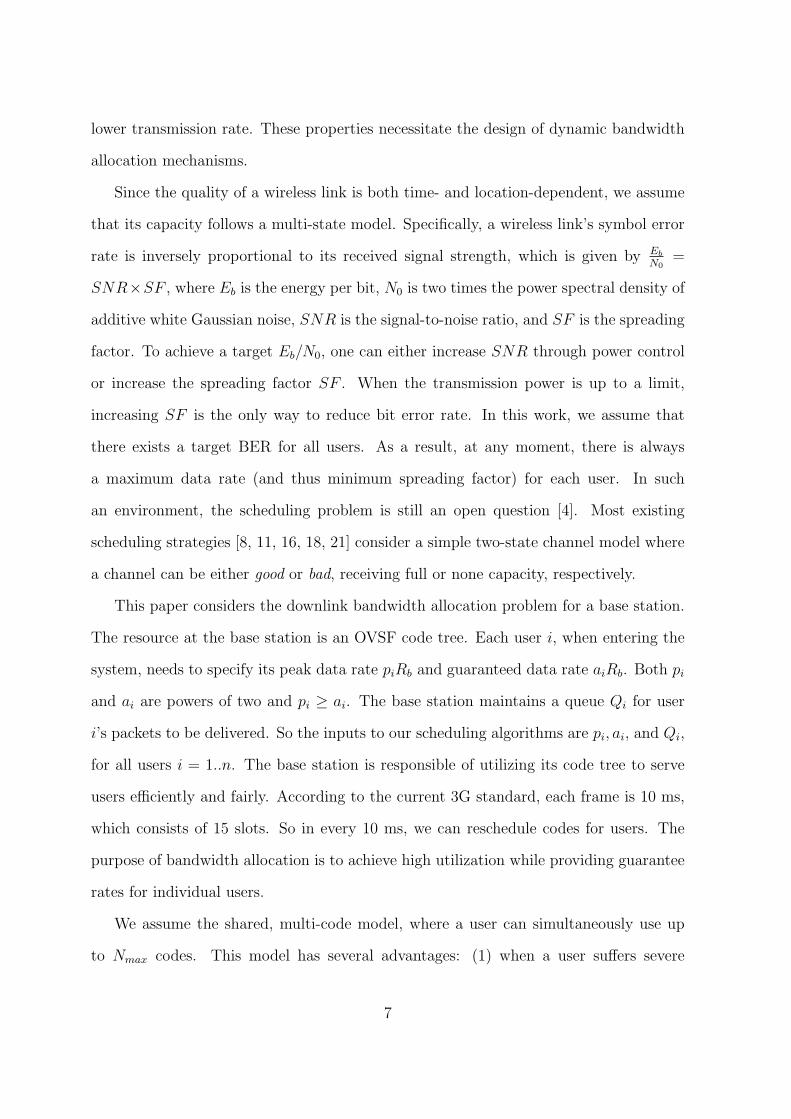
Figure 7: Transmitted transport blocks versus time under traffic model II.

(performance comparisons of different Nmax are not reported here due to space limit).

To see rate guarantee, we randomly choose a user i with request ai = 1, 2, 4, or 8Rb and

observe the number of transmitted transport blocks. As shown in Fig. 7, both schemes

2 and 3 support rate guarantee well. For scheme 1, there is some lag for ai = 4 and 8Rb,

which stems from the higher failure probabilities when allocating codes for such calls.

To verify access fairness, we introduce a metric called inter-service time, which is

the interval that a backlogged user experiences, measured in time frames, between two

successive transmissions. We observe the maximum difference of inter-service times of

two backlogged users who are waiting for scheduling. The result is in Table 2. In all

three traffic models, scheme 3 has the least difference, which is followed by scheme 2

and then scheme 1. For the constantly backlogged model, the differences are low for

all schemes and are proportional to traffic load. For example, at traffic load=80%, the

most unfortunate user will experience at most 15.1, 8.1, and 3.9 time frames of delay

for schemes 1, 2, and 3, respectively. For both bursty traffic models, the difference is

relatively independent to traffic load. Scheme 3 performs the best, and scheme 1 the

worst. In general, the differences are larger for the highly bursty traffic model, which is

21

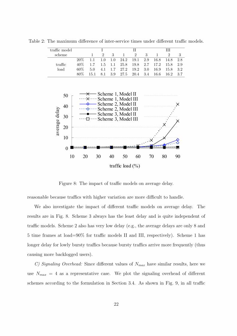
Table 2: The maximum difference of inter-service times under different traffic models.

traffic model I II IIIscheme 1 2 3 1 2 3 1 2 3

20% 1.1 1.0 1.0 24.2 19.1 2.9 16.8 14.8 2.8traffic 40% 1.7 1.5 1.1 25.8 19.8 2.7 17.2 15.8 2.9load 60% 5.0 4.1 1.7 27.2 19.2 3.0 16.9 15.8 3.2

80% 15.1 8.1 3.9 27.5 20.4 3.4 16.6 16.2 3.7

0

10

20

30

40

50

10 20 30 40 50 60 70 80 90

traffic load (%)

av

era

ge

dela

y

Scheme 1, Model IIScheme 1, Model IIIScheme 2, Model IIScheme 2, Model IIIScheme 3, Model IIScheme 3, Model III

Figure 8: The impact of traffic models on average delay.

reasonable because traffics with higher variation are more difficult to handle.

We also investigate the impact of different traffic models on average delay. The

results are in Fig. 8. Scheme 3 always has the least delay and is quite independent of

traffic models. Scheme 2 also has very low delay (e.g., the average delays are only 8 and

5 time frames at load=90% for traffic models II and III, respectively). Scheme 1 has

longer delay for lowly bursty traffics because bursty traffics arrive more frequently (thus

causing more backlogged users).

C) Signaling Overhead: Since different values of Nmax have similar results, here we

use Nmax = 4 as a representative case. We plot the signaling overhead of different

schemes according to the formulation in Section 3.4. As shown in Fig. 9, in all traffic

22

Scheme 1Scheme 2Scheme 3

sig

nali

ng o

verh

ead (

bit

s)

Model IModel II

Model III

traffic load (%)10

90

200

400

600

800

1000

1200

1400

050

1600

Figure 9: Signaling overhead of different schemes.

models, scheme 2 incurs the least signaling overhead while scheme 3 the highest. Note

that we should also take into account the utilization issue while evaluating these schemes.

When this factor is considered, scheme 2 will be the best for traffic models II and III. For

example, for model II under load = 90%, the signaling overheads are 152 and 720 bits

for schemes 2 and 3, respectively. The effective utilization of scheme 3 is only 1% higher

than scheme 2, which means around 1%×256×150 = 384 bits of reward at the expense

of 720− 152 = 568 bits of overhead when comparing scheme 3 and scheme 2. However,

for model I, scheme 3 performs the best when the utilization factor is considered.

D) Impact of Fully Shared Code Space for Scheme 2: Lastly, we investigate how the

ratio of fully shared code space in scheme 2 affects its performance. Four ratios, 18, 2

8, 3

8,

and 48, are tested with different Nmax values. Due to the space limit, we report the results

without figures. When Nmax = 2, the one with 28

fully shared code space performs the

best. As Nmax increases, larger ratios would be more beneficial. It is because calls can

more freely utilize the fully shared space, causing less blocking problem. When Nmax is

large enough to better utilize the fully shared space, the utilization would be the best.

23

(However, the advantage can not be seen when Nmax is too small.) When Nmax = 3 and

4, the one with 38

fully shared code space performs the best.

To conclude, we believe that a scheme does not consider channel condition, such as

the KMS scheme, may perform poorly. In our proposal, scheme 3 has the best behavior

in terms of utilization, delay, rate guarantee, and fair access. However, it also imposes the

highest signaling overhead. Scheme 2 falls behind scheme 1, but has the least signaling

overhead. Taking all these issues into account, we recommend to use scheme 3 under

constantly backlogged traffic model (Model I) and scheme 2 under bursty traffic models

(Model II and III) by properly tuning the fully shared code space depending on the

given Nmax.

5 Conclusions

Wireless bandwidth is a precious resource. Thus, resource management is an important

issue for WCDMA. Existing mechanisms supporting multimedia traffic either do not

consider channel condition or fail to address the exact code position in the code tree,

which may result in inefficiency in resource utilization. In this paper, we have proposed

three algorithms to provide fair and rate guaranteed service for multimedia traffic in

a WCDMA system. The essence of our protocols is a credit-based scheduler which

considers channel condition and explores the concept of compensation codes. With our

channel-sensitive scheduling algorithms, a user with more credits will have more chance

to transmit without compromising to the transmission quality. Simulation results do

justify that schemes 2 and 3 work well.

References

[1] Third generation partnership project; Technical specification group radio access net-

work. Spreading and modulation (FDD), http://www.3gpp.org, 1999.

24

[2] F. Adachi, M. Sawahashi, and H. Suda. ”Wideband DS-CDMA for next-generation

mobile communications systems”. IEEE Commun. Mag., 36:56–69, Sept., 1998.

[3] R. Assarut, K. Kawanishi, U. Yamamoto, Y. Onozato, and Masahiko. ”Region

division assignment of orthogonal variable-spreading-factor codes in W-CDMA”.

IEEE VTC 2001 Fall, pages 1184–1898, 2001.

[4] Y. Cao and V. O. Li. ”Scheduling algorithms in broad-band wireless networks”.

Proceedings of the IEEE INFOCOM, 89(1):76–87, Jan, 2001.

[5] C.-M. Chao, Y.-C. Tseng, and L.-C. Wang. ”Reducing internal and external

fragmentations of OVSF codes in WCDMA systems with multiple codes”. IEEE

WCNC, pages 693–698, 2003.

[6] W.-T. Chen, Y.-P. Wu, and H.-C. Hsiao. ”A novel code assignment scheme for

W-CDMA systems”. IEEE VTC 2001 Fall, pages 1182–1186, 2001.

[7] R.-G. Cheng and P. Lin. ”OVSF code channel assignment for IMT-2000”. IEEE

VTC 2000 Spring, pages 2188–2192, 2000.

[8] D. Eckhardt and P. Steenkiste. ”Effort-Limited Fair (ELF) scheduling for wireless

networks”. IEEE INFOCOM, pages 1097–1106, 2000.

[9] R. Fantacci and S. Nannicini. ”Multiple access protocol for integration of variable

bit rate multimedia traffic in UMTS/IMT-2000 based on wideband CDMA”. IEEE

Journal on Selected Areas in Communications, 18(8):1441–1454, Aug., 2000.

[10] V. K. Garg. IS-95 CDMA and cdma2000. Prentice Hall, 2000.

[11] J. Gomez, A. T. Campbell, and H. Morikawa. ”The Havana framework for sup-

porting application and channel dependent QoS in wireless networks”. ICNP, pages

235–244, 1999.

25

[12] H. Holma and A. Toskala. WCDMA for UMTS. John Wiley & Sons, 2000.

[13] C.-L. I et al. ”IS-95 enhancements for multimedia services”. Bell Labs. Tech. J.,

pages 60–87, Autumn, 1996.

[14] A. Z. Kam, T. Minn, and K.-Y. Siu. ”Supporting rate guarantee and fair access for

bursty data in W-CDMA”. IEEE Journal on Selected Areas in Communications,

19(12):2121–2130, Nov., 2001.

[15] D. Kandlur, K. Shin, and D. Ferrari. ”Real-time communication in multi-hop

networks”. ACM SIGCOMM, pages 300–307, 1991.

[16] S. Lu and V. Bharghavan. ”Fair scheduling in wireless packet networks”.

IEEE/ACM Trans. Networking, 7(4):473–489, 1999.

[17] T. Minn and K.-Y. Siu. ”Dynamic assignment of orthogonal variable-spreading-

factor Codes in W-CDMA”. IEEE Journal on Selected Areas in Communications,

18(8):1429–1440, Aug., 2000.

[18] T. S. E. Ng, I. Stoica, and H. Zhang. ”Packet fair queueing algorithms for wireless

networks with location-dependent errors”. INFOCOM, pages 1103–1111, 1998.

[19] A. Parekh and R. G. Gallager. ”A generalized processor sharing approach to flow

control in integrated services networks: The single-node case”. IEEE/ACM Trans.

on Networking, 1:334–357, June, 1993.

[20] J. G. Proakis. Digital Communications. McGraw-Hill, forth ed., 2001.

[21] P. Ramanathan and P. Agrawal. ”Adapting packet fair queueing algorithms to

wireless networks”. ACM/IEEE MOBICOM, pages 1–9, 1998.

26

[22] F. Shueh, Z.-E. P. Liu, and W.-S. E. Chen. ”A fair, efficient, and exchangeable

channelization code assignment scheme for IMT-2000”. IEEE ICPWC 2000, pages

429–436, 2000.

[23] Y.-C. Tseng and C.-M. Chao. ”Code placement and replacement strategies for wide-

band CDMA OVSF code tree management”. IEEE Trans. on Mobile Computing,

1(4):293–302, Oct.-Dec. 2002.

[24] J. Wigard, N. A. H. Madsen, P. A. Gutierrez, I. L. Sepulveda, and P. Mogensen.

”Packet scheduling with qoS differentiation”. Wireless Personal Communications,

23:147–160, 2002.

[25] L. Xu, X. Shen, and J. W. Mark. ”Dynamic bandwidth allocation with fair schedul-

ing for WCDMA systems”. IEEE Wireless Communications, 9(2):26–32, April,

2002.

[26] Y. Yang and T.-S. P. Yum. ”Nonrearrangeable compact assignment of orthogonal

variable-spreading-factor codes for multi-rate traffic”. IEEE VTC 2001 Fall, pages

938–942, 2001.

[27] L. Zhang. ”Virtual clock: A new traffic control algorithm for packet switching

networks”. ACM SIGCOMM, pages 19–29, 1990.

27