DYNAMIC AND STATIC FIELD TESTS ON A SMALL INSTRUMENTED PILE

by

Kenneth W. Korb

Research Assistant

and

Harry M. Coyle

Associate Research Engineer

Research Report Number 125-2

Bearing Capacity for Axially Loaded Piles

Research Study Number 2-5-67-125

Sponsored by

The Texas Highway Department

In Cooperation with the

U.S. Department of Transportation,

Federal Highway Administration,

Bureau of Public Roads

February 1969

TEXAS TRANSPORTATION INSTITUTE Texas A&M University College Station, Texas

i

T&chnlcal Reports Center TCICII Transportatiof11nstituf6

Preface The information contained herein was developed on Research Study 2-5-67-125

entitled "Bearing Capacity for Axially Loaded Piles" which is a cooperative research study sponsored jointly by the Texas Highway Department and the U. S. Department of Transportation, Federal Highway Administration, Bureau of Public Roads. The broad objective of this project is to develop a procedure whereby the bearing ca­pacity of an axially loaded pile can be determined for any combination of soil and driving conditions.

This is the second research report on this study. This report presents the results of a series of field tests which were conducted with a small instrumented pile. The small instrumented pile was used to measure dynamic and static skin friction and point loads in a variety of field soils. The soils at the test sites included clays of high and low plasticity and silty sands. The small pile was instrumented in such a manner that separate measurements of skin friction and point bearing were made simul­taneously.

A mathematical model in current use which describes the action of the pile-soil system during dynamic or static loading was examined. load test data were used to evaluate soil damping constants both in skin friction and point bearing in accord­ance with this model. The load test data were also used to evaluate the elastic deformation or quake of the soil and to determine the distribution of the total dynamic and static load between skin friction and point bearing.

A modification of the mathematical model was made in order to achieve a con­stant damping factor for skin friction in clays and point bearing in saturated sands. Conclusions are given regarding the practical application of test results in wave equation studies of piling behavior. The use of the soil parameters evaluated in this study should give better correlation when determining blow-count or driving resist­ance by the wave equation method.

The opinions, findings, and conclusions expressed in this report are those of the authors and not necessarily those of the Bureau of Public Roads.

ii

TABLE OF CONTENTS

LIST OF TABLES ... --------------------------------------------------------------------------------------------------------------------------····-·-------------------------------··-.iv

LIST OF FIGURES·--------------------------------------------------------·---------------------------------------------------------------·-···· ... ···-···-·-··---------------------- v

Chapter Page

I. INTRODUCTION .. ---------------------------------------------------------------------------------------------------------------------------------------------------------- 1

Background Information .. -------------------------------------·------------------------------------------------------------------------------------------------- 1

Present State of the Question .... ----------------------------------------------------------------------------------------------------------------------------- 1 Objectives __________________________________________________________________________________________________________________________________________________________________ -2

II. EQUIPMENT AND INSTRUMENTATION _____________________________________________________________________________________________________________ 3

GeneraL .... --------------------------------·------------------------------------------------------·------------------------------------------------------------------------- 3

The Small Instrumented Pile·--------------------------------------------------------------------------------------------------------------------------------- 3

Loading Equipment .... _.---------------------------------------------------------------------------------------------------------------------------------·--------- 4

Displacement Measurement .... ------------------------------------·-------------------------------------------------------------------------------------------- 4

Recording Equipment.·------------------------------------------·------------------------------------------------------------------------------------------------- 5

Calibration ............ ---------------------------------------------------------------------------------------------------------------------------------------------------- 6

III. TEST SITES.------------------------------------------------------------------------------------------------------------------------------------------------------------------- 7

Site Locations.--------------------------------------------------------------------------------------------------------------------------------------------------------- 7

Engineering Properties of the Test Soils .............. : ......... -------·------------------------------------------------------------------------------ 7

IV. TEST PROCEDURE .............. ----------------------------------------------------------------------------------------------------------------------------------------- 8

The Pilot Hole ..... -----------------------------------------------------------------------------------------------------------------·-··-------------------------------- &

Insta Uation of the Pile, ________________ .. -------------------------. _______ .................... ----------------------- __ ... ____________ ----------- .. ------------- 9

Dynamic Test Procedure------------------------------------·-------------------------------------------------------------------------------------------------- 9

Static Test Procedure ................ ----------------------------·-------------------------------------------------------------------------------------------------10 V. ANALYSIS OF TIP DAMPING DATA _______________________________________________________________________________________ : ______________________________ lO

Fine-Grained Soils ........... ----------------------------------------------------------------------------------------------------------------------------------------1l> Coarse-Grained Soils _______________________________________________________________________________________________________________________________________________ 11

VI. ANALYSIS OF FRICTION DAMPING DATA ........ -------------------------------------------------------------------------------------------------13

Fine-Grained Soils ......... ------------------------------------------------------------------------------------------------------------------------------------------13

Coarse-Grained Soils ........ : ............ ---------------------------------------------------------------------------------------------------------------------------14

VII. ANALYSIS OF OTHER DATA OBTAINED .. __________ ---------------------------------------------------------------------·--···----------------------15

Quake .. -------------------··-------------------------------------------------------------------------------------------·······-----------·-----------------------------------15

Load Distribution ..... -----------------------------------------------------------------------------------------------------------------------------------------------15 VIII. CONCLUSIONS AND RECOMMENDATIONS _________________________________________________________________________________________________________ 17

Conclusions ..... --;:--···--------·----------------------·-·:··------------------------------------------------------------------------------------------------------------17

Recommendations ............. -----------------------------------------------------------------------------------------------·---------------------------------------17

REFERENCES·--·-------------------------------------------------------------------------------------------------------------------------------------------------------------18

APPENDIX A-Load-Deformation Curves·----------------------------------------------------------------------------------------------------------------19

APPENDIX B-Data Reduction from the Visicorder Trace·----------------------------------------------------------------------------------24

iii

LIST OF TABLES

Table Page

I. Engineering Properties of the Test Soils. ..................................................................................................................... 9

II. Tip Damping Data for Fine-Grained Soils .................................................................................................................. ll

III. Tip Damping Data for Coarse-Grained Soils .................................................... , ......................................................... 12

IV. Friction Damping Data for Fine-Grained Soils .......................................................................................................... 13

V. Friction Damping Constants from Modified Smith Model .................................................................................... 13

VI. Friction Damping Data for Coarse-Grained Soils .................................................................................................. 14

VII. Quake Data from Field Test Program .......................................................................................................................... 15

VIII. Load Distribution Data ................................ -............................................................................................................ 16-17

iv

LIST OF FIGURES

Figure Page

l A Comparison of a Typical Pile Driving System with Smith's Idealization ______________ ,: __________________________________________ l

2 Assumed Soil Load-Deformation Characteristics---------------------------------------------------------------------------------------------------------- 2

3 Small Instrumented Pile·------------------------------------------------------------------------------------------------------------------------------------------------- 3

4 Load Frame·------------------------------------------·--------------------------------------------------------------------------------------------------------------------------_ 5

5 Static Loading Equipment---------------------------------------------------------------------------------------------------------------------------------------------- 6

6 Recording Equipment·----------------------------------------------------------------------------------------------------------------------------------------------------- 6

7 Typical Visicorder Trace ---------------------------------------------------------------------------------------------------------------------------------------------- 6

8 Bridge Calibration ---------------------------------------------------------------------------------------------------------------------------------------------------------- 6

9 Generator Calibration ______ _- _________________________________________________________ ·--------------------------------------------------------------------------------------- 7

10 Cohron Sheargraph and Typical Plot___ _______________________________________________________________________________________________________________________ 8

ll Test Site Layout------------------------------------------------------------------------------------------------------------------=------------------------------------------- 9

12 Setup for a Dynamic Test.·-------------------------------------------------------------------------------------------------------------------------------------------- 9

13 Setup for a Static Test. ________________________________________________ -------------------------------------------------------------------------------------------------10

14 J vs. Displacement Velocity in Fine-Grained Soils ____ ---------------------------------·---------------------------------------------------------------10

15 Tip Damping Constant vs. Pile Displacement Velocity in Coarse Soils ________________________________________________________________ l2

16 Friction Damping Constant vs. Pile Displacement VelocitY--------------------------------------------------------------------------------------13

17 J' from Modified Smith Model vs. Pile Displacement Velocity _______________________________________ -----------------------------------------13

18 Friction Damping Constants vs. Pile Displacement Velocity in Coarse-Grained Soils _________________________________________ l4

19 Frictional Load vs. Settlement in Coarse-Grained Soils --------------------------------------------------------------------------------------14

A-l Load-Deformation Curves ----------------------------------------------------------------------------------------------------------------------------------------------19

A-2 Load-Deformation Curves ----------------------------------------------------------------------------------------------------------------------------------------------19

A-3 Load-Deformation Curves -------------------------------------------- -------------------------------------------------------------------------------------------------20

A-4 Load-Deformation Curves --------------------------------------------·-------------------------------------------------------------------------------------------------20

A-5 Load-Deformation Curves ----------------------------------------------------------------------------------------------------------------------------------------------20

A-6 Load-Deformation Curves ------------------------------------------···-------------------------------------------------------------------------------------------------21

A-7 Load-Deformation Curves ----------------------------------------------------------------------------------------------------------------------------------------------21

A-8 Load-Deformation Curves ----------------------------------------------------------------------------------------------------------------------------------------------21

A-9 Load-Deformation Curves ----------------------------------------------------------------------------------------------------------------------------------------------22

A-10 Load-Deformation Curves ----------------------------------------------------------------------------------------------------------------------------------------------22

A-ll Load-Deformation Curves -------------------------------------------- -------------------------------------------------------------------------------------------------23

A-12 Load-Deformation C"urves ---------------------------------------------------------------------------------------------------------------------------------------------23

B-l Typical Oscillograph -----------------------------------------------------------------------------------------------------------------------------------------------------24

Bl2 Typical Static Load-Settlement Curves-------------------------------------------------------------------------------------------------------------------------24

v

NOTATION

The following notation was used in this report:

Pdynamic

Pstatic

c

J

J'

X

N

Wn

Tu

the peak dynamic resistance,

the peak static resistance,

additional soil resistance due to dynamic load,

a viscous damping constant in pound-sec­onds per foot,

a viscous tip damping constant, in seconds per foot,

a viscous friction damping constant, in sec­onds per foot,

the velocity of a pile segment in any time interval, in feet per second,

an exponent to which the loading velocity is raised,

liquidity index,

soils natural moisture content,

soils liquid limit,

soils plastic limit,

unconfined shear strength,

vi

e

Sr

n

Cu

sc SM

CH

CL Qt

shear strength obtained with Cohron Shear­graph,

soil's specific gravity,

void ratio,

percent saturation,

standard penetration blow count,

coefficient of uniformity,

- a clayey sand,

a silty sand,

a highly plastic clay,

a low plasticity clay,

the quake, or elastic deformation of the soil at the pile tip,

the quake, or elastic deformation of the soil at the side of the pile,

the total capacity of the pile,

the load carried at the pile tip,

the load carried by friction along the pile soil contact area,

the ratio Rt!Ru.

the ratio Rt/Ru.

Dynamic and Static Field Tests On A Small Instrumented Pile

CHAPTER I

INTRODUCTION

Background Information

The behavior of a pile-soil system when subjected to dynamic loads has generated considerable interest in recent years. With the advent of large marine struc­tures, it has become necessary to drive very long piles with large diameters. The driving of such large piles often proves difficult and inefficient. In some cases, destructive stresses have been generated in piles during the driving operation. A method of studying and pos­sibly solving some of these problems was suggested by E. A. L. Smith (8) * in 1962.

Present State of the Question

Smith (8) suggested a numerical method to analyze the pile driving problem. He used the passage of stress waves through the pile as the basis for his method. The mathematical model he suggested to describe the soil resistance when a pile is loaded dynamically is:

Pdynamic = Pstatlc (l + J~) (l)

where: P dynamic

Pstatic

the peak dynamic resistance,

the peak static resistance,

J . , a viscous tip damping constant used · '" ·when describing the soif resistance

at the tip. A viscous friction damp­ing constant J' is used when de­scribing the frictional resistance of

tR<J' the pile-soil system,

X the velocity of a pile segment in any time interval.

This mathematical model is more easily understood when Smith's idealization of a pile-soil system is exam­ined (see Figure l). It can he seen that all parts of the pile driving system are included in this idealized model. The pile driving ram, cushion, follow block, and the pile itself are all treated as lumped masses and springs. The soil's resistance is represented by springs, sliding blocks, and dashpots.

Assumed load-deformation curves for the soil are shown in Figure 2. Figure 2(a) is a curve representing the assumed static load-deformation characteristics of soil. The soil deforms ehlstically along line OA until the friction in the sliding block is overcome. The soil then deforms plastically along line AB. After the load is removed, the elastic portion of the deformation is regained along line BC. In the case of frictional resist-

*Numbers in parentheses refer to corresponding items in list of references. The citations on the following pages follow the style of the Journal of Soil Mechanics and Foundation Division, American Society of Civil Engi­neers.

ance, the soil then goes into tension, and is deformed elastically along line CD until the sliding block friction is again overcome. The soil then deforms plastically along line DE. At this point, the elastic tensile defor­mation is regained along line EF, and the cycle begins again. The lower or tensile portion of the curve does not apply for loads at the tip.

The slope of the elastic portion of the static curve is assumed to be the soil's spring constant (K). There­fore, the soil static resistance for any deformation (x) can be computed using:

P = Kx

When the soil is loaded dynamically, its load defor­mation curve is assumed to be similar to the one shown in Figure 2 (b) . The increased soil resistance is assumed to be due to the action of the dashpots, and is propor­tional to the velocity of soil deformation. Therefore, the load increase is:

ex

ijQ-RAM llZZ2I CUSHION-----

H-FOLLOW BLOCK-~...1...~

SEGMENT #1

SOIL SIDE

FRICTIONAL

RESISTANCE

Figure 1. A comparison of a typical pile driving system with Smith's idealization.

.PAGE ONE

·---·----~------------------------------------

0 c( 0 ....

0 c( 0 ....

T P STATIC

DEFORMATION

P STATIC

I t

P STATIC

DE FORMATION

P STATlC

l Figure 2. Assumed soilload·deformation characteristics.

where: Pa additional soil resistance due to dynamic load,

c a viscous damping constant,

x - the velocity of soil deformation for a given time interval in feet per second.

Therefore, the total dynamic soil resistance is:

P dynamic = Kx + ex

In an attempt to take the pile's size and shape into consideration, Smith let:

c = Kx(J or J')

where: J a viscous tip damping constant,

J' a viscous friction damping constant.

therefore: P dynamic Kx + Kx J~

Kx (1 + Jx)

PAGE TWO

The maximum static soil resistance is:

Pstatlc = QK

where: Pstatlc the maximum static soil resist· ance,

Q the maximum elastic deformation or quake of the soil.

The maximum dynamic soil resistance is therefore:

Pdynamic = Pstauc [1 + (J or J')~] (1)

where: P dynamic the- maximum dynamic soil resistance, the viscous damping constant used when computing the maxi· mum soil resistance at the tip of the pile,

J' = the viscous damping constant used when computing the maxi­mum frictional soil resistance.

When Smith proposed this model, he recommended values to be used for the soil constants involved. He recommended that a value of 0.15 be used for J, and that J' should be assumed to be about one-third of J, or 0.05. He also suggested that a value of 0.10 be used for the soil's quake.

Samson, Hirsch, and Lowery (6) (7) adopted Smith's method so that the driving of a pile could be simulated on the large high speed digital computer. Chan ( 1) and Reeves ( 5) conducted both dynamic and static loading tests on specially prepared samples in order to obtain information about the viscous damping properties of sands. Raba ( 4) conducted a laboratory investigation of the friction damping properties in re­molded clay samples, and related these damping proper­ties to several common soil parameters.

Gibson (3) did laboratory research on the damping properties of sands and clays. His research indicated that if some modifications were made to Smith's mathe­matical model, truly constant values of viscous damping could be obtained for any loading velocity. Gibson's modification of Smith's model is:

Pdynamic = Pstatlc (1 + J~N) (2)

where: N = an ·exponent to which the loading velocity is raised. This exponent varies with soil type.

It can be seen that a considerable amount of labora· tory work has been done in order to obtain representa­tive values of soil viscous damping constants. To date, all work has been done on specially prepared soil sam­ples, and no effort has been made to examine the inter· action between friction and tip damping for the actual field situation.

Objectives

The objectives of this investigation are: (1) to de­sign and fabricate a small instrumented pile and the necessary equipment to conduct loading tests, (2) to conduct a field test program to include both static and dynamic loading tests, and ( 3) to evaluate soil damping constants, elastic soil deformation or quake, and distri­bution of load between skin friction and point bearing in the soils tested.

CHAPTER II

EQUIPMENT AND INSTRUMENTATION

General

In order to obtain the desired data, a small instru­mented pile was needed. Since both friction and tip damping were studied, a pile capable of measuring both side friction and tip loads was required. Loading equip­ment capable of applying both variable velocity dynamic loads and static loads was also required. Electronic equipment was needed which could record applied load and pile displacement for both the dynamic and static load tests.

The Small Instrumented Pile

V esic ( 9) conducted a series of model pile tests in sands. He used a model pile constructed on the princi­ple of deep cone penetrometers. It consisted of an outer tubular shaft, and a piston like tip connected to an inner shaft. This principle was used in the design of the pile used in this study. (See Figure 3.)

The upper 20.5 in. of the outer shaft was constructed of extruded 606l-T6 aluminum tubing with an outside diameter of 2.5 in. and a wall thickness of .125 in. A joint was made four inches from the top of the outer shaft in order to accommodate a linear ball bushing. This bushing is 4 in. in length, and the joint was ac­complished by press fitting the two four in. sections of outer shaft onto either end of the bushing until the two sections were joined.

Overlapped joints with four screw connectors were used at points 8 in. and 16 in. below the top of the outer shaft. The primary reason for these joints was to ease strain gauge application.

The bottom 3.5-in. section of the outer shaft was constructed of 2.5-in. O.D. stainless steel tubing. This tubing had a wall thickness of 0.083 in. and was jointed to the aluminum by the use of an overlapped joint. A cutting edge was machined at the tip of this stainless steel section at a 30o angle. This was done in order to minimize tip load pickup at the lower edge of the outer shaft. A l-in. long cantilever was attached l in. from the top on the outer shaft. This cantilever served the purpose of an anchor for the device which measured vertical displacement.

The top 18.5 in. of the inner shaft consisted of an unjointed section of 1.5-in. O.D. SMLS 304 stainless steel tubing with a wall thickness of 0.065 in. The upper portion of this inner shaft rides in the linear ball bushing mentioned earlier. The lower 3 in. of the inner shaft consists of a section of 1.5-in. outside diameter extruded 606l-T6 aluminum tubing .with a wall thickness of 0.065 in. The joint between these two sections is an over­lapped joint with a 1.57-in. diameter, 0.5-in. long, and 0.125-in. thick stabilization ring inside the shaft and secured with three screws. A 2.1-in. diameter aluminum base plate was attached to the inner shaft by means of a threaded connection. To obtain the piston effect at the tip, a 3-in. long section of 2.324 in. O.D. stainless steel tubing was press fitted onto the aluminum base plate. The gap between the piston tip and the outer

N1fSS run

ALUMINUM

TUBE 6 ~ .... '

Figure 3. Small instrumented pile.

P'AGE THREE

r--------------------------------------------------------------------------------------------------------------------

shaft was sealed by the use of a teflon "0" ring which was seated in a machined groove. This groove is 0.125 in. from the bottom on the inside of the outer shaft.

A 1.5-in. long cantilever was attached 0. 75 in. from the top of the inner shaft 180 degrees from the cantilever attached to the outer shaft. This cantilever also serves as an anchor for the measurement of displacement for the inner shaft. In order for this cantilever to extend outside the outer shaft, and to have freedom of vertical movement, a 0.375-in. by 1.0-in. slot was cut in the outer shaft.

Four 90-degree Budd SR-4 strain gage rosettes were mounted 90 degrees apart on the inner surface of the outer shaft. They were placed 10 in. from the top of the outer shaft. These gauges were then wired to read only axial loads. A similar gauge arrangement was also mounted on the inner surface of the inner shaft 1 in. from the bottom.

The pile was designed to enable the tip and inner shaft to move relative to the outer shaft and vice-versa. The original plan was to load the tip and side separately. Preliminary dynamic tests showed, however, that when the tip and frictional loads obtained by separate meas­urements were compared with the simultaneous measure­ments, the totals and the distributions were different. For example in sand the separate frictional load was 280 pounds and the separate tip load was 575 pounds for a total of 855 pounds. Simultaneous measurements in sand yielded 60 pounds in friction and 775 pounds in tip load for a total of 835 pounds. In clay, the sep­arate frictional load was 420 pounds and the separate tip load was 180 pounds for a total of 600 pounds. Simultaneous measurements in clay yielded 350 pounds in friction and 140 pounds in tip load for a total of 490 pounds. From these figures it can be seen that the two methods of measurement yielded considerably dif­ferent results.

It was concluded that the interaction between tip and frictional loads was responsible for the results ob­tained in the preliminary tests. It was further concluded that in order to obtain conclusive data, separate but simultaneous measurements of tip and frictional resist­ance must be made. A three-piece aluminum cap was designed to accomplish this separate and simultaneous load measurement. It enabled the pile tip to be extended slightly beyond the end of the outer shaft. This ar­rangement enabled the gages mounted on the outer shaft to measure only the strain induced by frictional load on the outer shaft. Likewise, the gages mounted on the inner shaft measured only strain induced by load at the tip. This three-piece cap is shown in Figure 3.

Loading Equipment

In order to obtain the desired data, it was felt that the loading equipment should possess at least the fol­lowing characteristics:

l. 'It should be massive enol\gh to conduct static load tests.

2. It should be capable of applying variable mass and variable velocity dynamic loads to the small pile.

3. It should be simple.

4. It should be portable enough for two men to handle.

PAGE FOUR

The first and last specifications listed above were very difficult to fulfill simultaneously. It was estimated that the pile-soil system would experience static load in the 1000-pound to 1500-pound range in some soils. This meant that the loading equipment would have to be anchored, which would seriously limit the number of tests possible. The other possible solution was to make the loading equipment heavy enough to resist these large static loads. This would hinder its portability.

The design finally used was that of the load frame shown in Figure 4. The two vertical members were 6 WF 15.5, 6 ft. in length. A 20-in. by 20-in. by 0.50-in. plate was welded to the bottom of each vertical member.

The top horizontal member is an important com­ponent of the dynamic loading system. It consists of a 32-in. long 4 WF 13 member with two 6-in. by 6-in. by 0.50-in. plates welded on both ends. These plates are drilled and serve as a mounting bracket when this hori­zontal member is bolted between the two vertical mem­bers. A spherical ball bearing is mounted at the mid­point of this member (Figure 4a).

This bearing acted as the guide for a 5-ft. long, 0.50-in. diameter hardened stainless steel shaft. The ball and socket makes it possible to adjust the plumb of this stainless steel shaft. A 50-pound weight with a 1.5-in. diameter, 1.05-in. thick stiff neoprene rubber striker head was attached to the end of this stainless steel shaft (Figure 4b). This assembly acted as the dynamic load­ing mechanism, or simulation of the pile driving ham­mer. The weight was released to strike the pile with a special trip mechaJ?.ism.

The static load test was accomplished by bolting a 6 WF 15.5 bottom horizontal member between the two vertical members. This horizontal section acted as a reaction member. The total weight of this frame was approximately 300 pounds. Since total loads of 1500 pounds were expected, the weight of the frame was not sufficient to react against. To solve this problem and continue to maintain the frame's portability, it was necessary to design some easily moveable weights which could become an integral part of the static load reaction frame. Ten 18-in. by 18-in. by 6-in. reinforced concrete weights were constructed with a 6-in. by 6-in. slot in one side. Stirrup shaped reinforcing steel bars were extended from the sides of these weights and were used as handles. The weights were 150 pounds each for a total possible 1500 pounds. These weights were stacked on the base plate with the vertical members of the frame fit into the 6-in. by 6-in. slot. These additional weights gave the frame a possible reaction of approximately 1800 pounds.

An Allstate 1.5-ton capacity hydraulic jack with an attached 10,000 pound capacity proving ring and dial gauge were used to apply the static load (see Figure 5).

Displacement Measurement

Since one of the variables in Smith's mathematical model is displacement velocity, it was necessary to obtain the pile's displacement velocity during impact loading. Load-displacement data were also needed to determine the soil's elastic and dynamic quake.

A Sanborn Model 7DCDT-1000 linear displacement transducer was used to obtain the required displacement data. The output signal of the transducer is proportional

------ ---------------------------------------------------------------------------------------------------

to the distance traveled by a high flux density permanent magnet through the bore of a differentially wound coil. Virtually no frictional resistance was imparted to the system by the transducer's operation. The transducer shaft was anchored to the cantilevers mentioned earlier. The transducer itself was mounted on a specially de­signed bracket.

DYNAMIC TESTS

DROP ASSEMBLY

\ \

STAINLESS STEEL SHAFT

HYDRAULIC

PROVING Rl NG

IIIII

MAIN LOAD FRAME

Recording Equipment A modelll9 Carrier Amplifier System and a Honey­

well 1508 Visicorder Oscillograph which were used to record the test data are shown in Figure 6.

The signals from the two strain gage bridges were fed into the bridge balance unit and amplifier. The am-

DROP ASSEMBLY

iPPORT FRAME

-

STATIC REACTION

MEMBER

STATIC LOAD

" , a

" , b

HAMMER ASSEMBLY

Figure 4. Load frame.

PAGE FIVE

Figure 5. Static loading equipment.

plified signals were then fed into the Visicorder. The sig­nal from the linear displacement transducer was fed into a calibration unit, then into the Visicorder.

Kodak Linograph Direct Print Light sensitive paper

Figure 6. Recording equipment.

PAGE SIX

7 11

SLOPE = [ ISPLAC EMENT 1/ H TIME LINES VELO CITY / \\ -

/ ~

-0.0[5£( I- !.-.. / 7

\ J ~\

Figure 7. Typical visicorder trace.

DISP LACEMENT

F RICTION LOAD -

-' Tl P OAD

was used in the Visicorder to record the data. The paper speeds used were 0.1 in. per second for static tests and 80 in. per second for dynamic tests. A sample visicorder trace for a dynamic test is shown in Figure 7.

Calibration Calibration of the system was accomplished in sev·

eral ways. It was first necessary to determine the lineari­ty of the strain gauge output. This was accomplished by loading the bridges separately in an lnstron loading machine and measuring the strain with a Budd SR-4 digital strain indicator. The resulting load-strain curves were plotted and were found to be linear.

The next step in calibration was to balance the strain gage bridges using the Honeywell bridge balance

Figure 8. Bridge calibration.

Figure 9. Generator calibration.

unit and carrier amplifier. A known weight was then applied to one of the bridges (see Figure 8), and the amplifier gain adjusted so that this known load caused the Visicorder trace to deflect a convenient distance. The weight was then removed, and an external calibra­tion resistance was plugged into the circuit and the deflection of the trace was noted. The same procedure was then followed on the other bridge. Throughout this test program, a l-in. trace deflection was calibrated to represent a 200-potind load on the tip bridge and a 400-pound load on the skin friction bridge.

After the above procedure had been followed, all that was required to calibrate the system was to balance the bridges, plug the calibration resistance into each cir­cuit, and adjust each amplifier's gain until the previ­ously noted trace deflections were obtained for each circuit.

Calibration of the linear displacement transducer was accomplished by moving the magnetic core through a known distance as observed on an Ames dial indicator. The trace deflection was then adjusted using a variable resistance until a convenient scale was obtained. Throughout this test program, a l-in. trace deflection was calibrated to represent a 0.1-in. pile displacement.

The power source, a 2.5-Kilowatt gasoline powered generator, was calibrated to insure an operating fre­quency of 60 cycles per second. This was accomplished by checking the time required for the second hand on an electric clock, which was powered by the generator, to make a full revolution. (See Figure 9.) If more than 60 seconds were required, the generator was running at a frequency less than 60 cycles per second, and the R.P.M. of the gasoline engine had to be increased. Adjustments of the engine speed were made by manipu­lating the throttle.

CHAPTER III TEST SITES

Site Locations

A preliminary site location survey was conducted in order to locate a variety of soils in which to test. It was desirous to test in soils ranging from highly plastic clays to sands.

Eleven locations yielding a reasonable variety of soils were located in the vicinity of Bryan, Texas. The site locations and the unified soil classifications are as follows:

l. The north side of F.M. Road 1687, approxi­mately 3 miles east of its intersection with Old San Antonio Road. Soil type-SC.

2. Fifty feet east of ~ite l. Soil type-SC.

3. The north side of F.M. Road 1687, approximate­ly :Y2 mile east of its intersection with F.M. Road 50. Soil type-CH.

4. Approximately 1 mile east of Site 3. Soil type -CH.

5. Adjacent to a pond at the southwest corner of the Texas A&M Research Annex. Soil type-SC.

6. Approximately 100 yards north of Site 5. Soil type-CL.

7. A lot east of the Texas Transportation Institute nondestructive test pavement section on the south end of the Research Annex. Soil type-CH.

8. West of a pond on the north end of the second runway at the Research Annex. Soil type-SM.

9. The west side of F.M. Road 50 approximately 4 miles south of its intersection with State Highway 21. Soil type-CL.

10. The south side of F.M. Road 1687 approxi­mately lf4 mile west of Sites 1 and 2. Soil type-SM.

11. The east side of State Highway 30 approxi­mately 4 miles south of its intersection with F.M. Road 158. Soil type-SM.

Engineering Properties of the Test Soils One of the purposes of this study was to compare

the damping constants obtained with several common soil parameters. In order to accomplish this purpose, a number of properties were determined for each soil tested.

PAGE SEVEN

NORMAL STRE 55 ~p s (a) (b)

Figure 10. Cohron sheargraph and typical plot.

In the fine-grained soils, such properties as liquidity index (I1), natural moisture content ( wn), percent satu­ration ( S,.), and shear strength ( r) were determined. In the coarse-grained soils, the percent saturation (S,.), standard penetration blow count (n), and the coeffi­cient of uniformity (Cu) were determined.

In all cases, accepted standard procedures were used to determine the properties for each soil tested. The only unusual procedure in this program was that used to obtain the in-situ shear strength ( rc) at the various sites. A Cohron (2) Sheargraph, marketed by Soiltest, Incorporated, was used for this purpose. This device

plots the normal pressure applied in pounds per square inch versus the soil shear strength in pounds per square inch. A Mohr failure envelope is obtained, and values of cohesion (c) , and angle of internal friction ( cp) can be obtained. Figure lOa shows a picture of the device. A sample sheargraph is shown in Figure lOb.

A summary of the engineering properties of all the soils is given in Table I. The analysis of test data re­vealed that it was not possible to correlate damping constants with any one soil parameter. The data in Table I are presented so that the reader can see the wide range of soil properties involved in the test sites.

Table I

Site % Passing Wn No. #200 Sieve %

1 41.2 26.0 2 22.4 21.1 3 95 36.6 4 94 37.8 .5 27.8 19.9 6 85 25.6 7 85 27.8 8 27.5 9.6 9 100 24.5

10 22.4 22.5 11 45 6.6

The Pilot Hole

ENGINEERING PROPERTIES OF THE TEST SOILS

W1 Wp % %

63.8 21.1 60.0 15.8 76.2 32.2 84.8 33.6 38.8 18.0 47.2 21.4 59 26.9 29.5 22.1 32.5 22.5 30.1 23.0 28.7 24.2

Tc

Tu c I1 psi psi

.885 13.4 3

.88

.9 13.95 10.8

.935 7.12 8.8

.91 14.75 3

.84 10.88 8.2

.975 5.77 6.6 2

.80 8.35 2 2.5 2

CHAPTER IV TEST PROCEDURE

"' G, e

45° 2.532 .48 2.525

8.5° 2.53 .81 5.2° 2.53 1.22

48° 2.615 .54 14° 2.50 .55 31° 2.475 .72 33° 2.625 .725 41° 2.60 .653 33° 2.652 .90 42° 2.650 .68

Unified . Soil

s n Cu Class.

91.0 sc sc

88.6 CH 48.7 CH 74.5 sc 93.0 CL 70.6 CH 21.1 8 36.7 SM 71 CL 42.6 6 19.5 SM 16.3 12 30.3 SM

During preliminary tests, it became apparent that the insertion of the small instrumented pile would be

impossible without some sort of pilot hole. The pile is relatively fragile and would have been torn apart under the repeated impact loads it would receive during actual

PAGE EIGHT

so"

-'\ -"\ -j -HOLE I) HOLE 2) HOLE 3 HOLE 4) 3"

6"

9"

6"

9" 9"

STATIC* STATIC* STATIC* STATIC*

* NOT RUN IN COARSE GRAINED MATERIAL

Figure 11. Test site layout.

I

driving. Also, it was felt that the instrumentation would not have held up under repeated dynamic loads.

Other investigations have us~d pilot holes in con­nection with their test programs. Raba ( 4) used a 0. 75-in. diameter pilot hole before inserting his l in. diameter pile in the soil sample. He found that this pilot hole did not affect the results of his tests signifi­cantly.

For this study, a 7-in. deep, 1.5-in. diameter pilot hole was used at all sites involving fine-grained soils. The pilot hole to pile diameter ratio which Raba ( 4) used was 0.75/l.O or, the pilot hole diameter was 75 percent of the pile diameter. The ratio used during this test program was 1.50/2.50 or, the pilot hole diameter was 60 percent that of the pile diameter. It may be assumed therefore, that if the pilot hole Raba ( 4) used did not affect his results, the pilot hole used in the fine­grained soils during this test program probably did not seriously affect the results contained herein.

In the coarse-grained soils tested, it was necessary to cut a pilot hole which had the same diameter as the pile. It was also necessMy to cut this pilot hole to the same depth as the planned depth of insertion. This was 8 in. in all cases.

The pilot holes did serve a useful purpose other than easing pile insertion. Two moisture samples were taken from each core obtained, and the remainder of the core was kept for laboratory use in classification and determining the engineering properties of the soils (Table I).

Installation of the Small Pile

Prior to digging the pilot hole, a hole 4 in. in diam­eter and 8 in. deep was augered at the side to be tested. This hole was dug in an attempt to remove the dry upper crust and organic material at the surface. The pilot hole was then dug to the depth needed for pile insertion.

In all cases, the pile was jacked to a penetration of 8 inches into the soil. Care was taken during this jack­ing procedure to insure that the pile was properly aligned vertically.

Since it was necessary in the coarse-grained soils, to use a pilot hole with the same diameter as the pile, an attempt was made to densify the soil around the pile in order to better simulate the actual soil conditions during driving. This was done by dropping the ham­mer onto the pile from a height of 6 in. The soil around the pile was then tamped with a small hammer in an attempt to accomplish this densification.

Dynamic Test Procedure

A standard test series was conducted at each test site. The pile was tested in four different holes (see Figure ll) . After insertion into the first hole, a series

Figure 12. Setup for a dynamic test.

PAGE NINE

Figure 13. Setup for a static test.

of dynamic tests was run. The test set-up for the dy­namic test is shown in Figure 12. This test series in­cluded a 3-in. hammer drop, a 6-in. drop, and a 9-in. drop. After this dynamic series was completed, a static test was run on the pile. The pile was removed and inserted into Hole 2. A dynamic test series consisting of a 6-in. and a 9-in. drop was conducted. A static test was then run on the pile. The pile was removed and inserted into Hole 3. A test series consisting of a 9-in. drop and a static test was then run. The pile was re­moved, inserted into Hole 4, and a static test was run. This concluded the test program at a given site.

This procedure was modified in the coarse-grained soils in that only one static test was run, and it was run in Hole 4.

Static Test Procedure As was mentioned in the previous section, several

static tests were run at each site. The procedure fol­lowed when conducting these static tests was as follows:

1. The static reaction member was bolted into the load frame assembly.

2. The bridges and transducer were balanced and calibrated.

3. The hydraulic jack and proving ring were then centered on the pile. The static test set-up is shown in Figure 13.

4. A 50-pound load was then applied to the pile and held for 2 minutes after which time an additional 50 pounds was applied. This load application procedure was continued until failure occurred.

During both the dynamic and static tests, both strain gage bridges and the displacement transducer were moni­tored, and the data were recorded.

CHAPTER V

ANALYSIS OF TIP DAMPING DATA

Fine-Grained Soils The terms fint<- and coarse-grained soils will be used

in the following discussion on analysis of test data. It would seem advantageous to define their meaning at this time. A slight departure is made from the defini­tions used in the. Unified Soil Classification System. In this study, the term fine-grained soils is used to signify clays (CL or CH) and clayey sands (SC). The term coarse-grained is used to signify silty sands (SM). The (SC) materials are considered fine-grained because the

· clay seems to be the dominant factor influencing the results.

The tip damping properties of all fine-grained soils ( CL, CH, SC) tested will be analyzed in this section. Smith's mathematical model as presented in Chapter I was used to determine these damping constants. With the data obtained from the test program, the tip damping constant (J) was calculated using:

PAGE TEN

Pdynamic- 1

J = Pstatic

X

(3)

Table II shows the data obtained in the field test program, and the values of J calculated using Equation 3. The values of Pst tlhown in Table II are values oh-. tained from the static test at that particular hole. Figure 14 shows the values of J from Table II plotted versus the displacement velocity of the pile. It is apparent that J

.s

.4

·.3

.2

D 0 2 3 4

DISPLACEMENT VELOCITY (1.~~

0 HOLE.l A HOLE 2

e HOLE 3

0 6 EXPONENT REPRESENTS SITE NUMBER

Figure 14. ! versus displacement velocity in fine-grained soils.

Table II

TIP DAMPING DATA FOR FINE-GRAINED SOILS

Site & Height Pdy P,, Hole of Drop (pounds) (pounds)

1-1 3" 420 355 1-1 6" 500 355 1-1 9" 550 355 1-2 6" 560 420 1-2 9" 590 420 1-3 9" 550 340

2-1 3" 380 340 2-1 6" 460 340 2-1 9" .510 340 2-2 6" 390 300 2-2 9" 450 300 2-3 9" 560 400

3-1 3" 270 180 3-1 6" 310 180 3-1 9" 340 180 3-2 6" 330 185 3-2 9" . 340 185 3-3 9" 330

4-1 3" 170 90 4-1 6" 205 90 4-1 9" 230 90 4-2 6" 225 145 4-2 9" 285 145 4-3 9" 280 115

5-1 3" 5-1 6" 690 630 5-1 9" 770 630 5-2 6" 755 710 5-2 9" 850 710 5-3 9" 800 680

6-1 3" 285 205 6-1 6" 320 205 6-1 9" 360 205 6-2 6" 320 190 6-2 9" 365 190 6-3 9" 385 185

7-1 3" 200 140 7-1 6" 240 140 7-1 9" 260 140 7-2 6" 230 125 7-2 9" 270 125 7-3 9" 260 130

9-1 6" 790 560 9-1 9" 820 560 9-2 6" 800 615 9-2 9" 900 615

is relatively constant for all of the fine-grained soils tested, and that a value of J equal to 0.15 sec/ft. would seem acceptable.

Gibson (3) found it necessary to modify Smith's model in order to obtain constant values of J in fine· grained soils. He found that by raising velocity to a power (see Equation 2) this could be accomplished. Gibson ( 3) obtained values of J ranging from 0. 7 to 1.25, and they seemed to be related to the liquidity index of the soil tested. Gibson ( 3) obtained these J values by raising the velocity to the 0.18 power. The variation in results could be explained by the fact that Gibson ( 3)

Pile Displacement J

Pdy/P,. Velocity (fps) (sec/ft.)

1.18 .083 .216 1.41 1.92 .214 1.55 3.48 .158 1.33 1.50 .220 1.40 2.78 .144 1.62 2.69 .231

1.12 1.10 .109 1.35 2.29 .153 1.50 3.68 .136 1.30 2.56 .117 1.50 4.17 .120 1.40 3.42 .117

1.50 1.86 .269 1.72 3.50 .206 1.89 4.20 .212 1.78 3.12 .250 1.84 4.00 .210

3.67

1.89 2.79 .319 2.28 4.45 .288 2.56 5.75 .272 1..55 3.37 .163 1.96 4.34 .221 2.44 5.33 .270

1.10 0.77 .131 1.22 1.56 .141 1.06 0.83 .072 1.20 1.00 .200 1.18 1.42 .127

1.39 2.17 .180 1.56 4.13 .136 1.75 5.33 .141 1.68 3.33 .204 1.92 4.75 .194 2.08 4.79 .226

1.43 2.21 .195 1.72 4.66 .154 1.86 7.00 .123 1.84 3.76 .224 2.16 5.16 .224 2.00 5.00 .200

1.41 1.96 .209 1.46 3.08 .149 1.30 1.63 .184 1.46 2.26 .204

did his work in the laboratory, and that his tests did not really simulate the action at the tip of a pile.

Coarse-Grained Soils

The tip damping data obtained in the coarse-grained soils (SM) were analyzed using Equation 3. Table III shows the data, and the values of J obtained. Figure 15 is a plot of the J values from Table III plotted versus the displacement velocity of that particular test. It can be seen that there is a large variation in results, and in some cases, negative values of J are obtained. It should be noted that percent saturation for field sites 8, 10,

PAGE EL.EVEN

Table III

TIP DAMPING DATA FOR COARSE-GRAINED SOILS

Site & Hole

8-1 8-1 8-1 8-2 8-2 8-3

10-1 10-1 10-1 10-2 10-2 10-3

11-1 11-1 11-1 11-2 11-2 11-3

LAB-1 LAB-1 LAB-1 LAB-1 LAB-1

3.0

2.0 I I

Height of Drop

3" 6" 9" 6" 9" 9"

3" 6" 9" 6" 9" 9"

3" 6" 9" 6" 9" 9"

%" Ph" 3" 6" 9"

P.y Pst (pounds) (pounds)

160 770 260 770 260 770 240 770 420 770 100 770

620 260 700 260 700 260 450 260 535 260 540 260

580 775 840 775 890 775 910 775 950 775 960 775

470 290 690 570 990 770

1340 1000 1300 1200

0

1.0

I I \ \ \ \

' ' ' '

10 []

'0- -- _0u II (.')JI d' Z>olr- -A- -t:::Y---

J 0~------------~------------~----

-LO

-20

-3.0

0

8 0

8 ~8

8 []

EXPONENTS REPRESENT SITE NUMBER

o HOLE I

A HOLE 2 c HOLE 3

0 LAB TEST (SATURATED OTTAWA SAND)

.5 1.0 1.5 DISPLACEMENT VELOCITY ( FPS)

Figure 15. Tip damping constant versus pile displace­ment velocity in coarse soils.

PAGE TWELVE

Pile Displacement J

P.y/P,. Velocity (fps) (sec/ft.)

.208 0.25 -3.16 .338 0.38 -1.77 .338 0.67 -0.99 .213 0.38 -1.84 .545 0.58 -0.78 .130 1.00 -0.87

2.38 0.75 1.84 2.69 0.81 2.04 2.69 0.97 1.74 1.73 0.62 1.17 2.06 0.92 1.15 2.08 1.17 0.92

0.75 0.56 -.450 1.08 0.77 .104 1.15 1.12 .134 1.17 1.10 .155 1.23 1.32 .174 1.25 1.54 .156

1.62 0.33 1.88 1.21 0.66 0.32 1.28 0.92 0.31 1.34 1.50 0.22 1.08 1.50 0.05

and ll varied from 16% to 42%. These percentages were considered low compared to what might be expected in sands below the water table in the field. Therefore, a series of tests was conducted in saturated Ottawa Sand in the laboratory. The results of these tests are given in Table III and plotted on Figure 15. The dashed curve on Figure 15 shows J values similar to those obtained by Gibson (3).

Gibson ( 3) ran a series of static and dynamic load tests on saturated sand samples. He found that by using the modified mathematical model (Equation 2) he could obtain relatively constant values of J for the sands tested. His results indicated that the best value of N to use in Equation 2 was about 0.20. The constant J values he obtained were J. = 0.92 for Ottawa Sand and l = 0.46 to 0.50 for the field sands he tested.

Static and dynamic Load-Deformation curves for both tip load and skin friction can he found in Appendix A. An examination of the static curves for the pile's tip from the coarse·grained soils (SM) reveals that these soils do not exhibit the elasto·plastic failure character­istics that Smith assumed (see Figure 2).

CHAPTER VI ANALYSIS OF FRICTION DAMPING DATA

Fine-Grained Soils

The friction damping data from the eight sites involving fine-grained soils was analyzed using Equa­tion l. Only the first dynamic test in each hole was used when analyzing the data from a particular site. This means that the P dynamic values and the velocities from the 3-inch drop in Hole 1, the 6 inch drop in Hole 2, and the 9-inch drop in Hole 3, were used in this analysis. In most cases, the P static values used were the average values for the sites. In some cases, where the Pstatic value varied considerably, the value of Pstatic from each hole was used.

Table IV shows the friction damping data, and the values of J' obtained using Equation l. These values of J' are shown plotted versus the pile's displacement velocity in Figure 16. It can be seen that a band of points is obtained. A curve is drawn in an attempt to best fit the data. Several points are taken from this

d th p dynamic . • d • h h curve an e P rahos associate Wit t ese static

points are found. The modified Smith model (Equation 2) is then used to obtain a constant value of J' using the ratios mentioned above. The data used in this pro­cedure are shown in Table V. Figure 17 is a plot of the friction damping constants (J') obtained by the above procedure plotted versus the pile's displacement velocity. The value of N used in Equation 2 was 0.35, and the average value of J' obtained was about 1.25.

Table IV FRICTION DAMPING DATA FOR FINE-GRAINED

SOILS

Displacement Velocity

Site Drop Pdy P,t (fps) J'

1 3" 680 350 0.83 1.13 1 6" 840 350 1.50 0.93 1 9" 880 350 2.69 0.56

2 3"" 640 2.50 1.10 1.42 2 6" 740 250 2.56 0.76 2 9" 880 250 3.42 0.74

3 3" 560 235 1.86 0.74 3 6" 780 235 3.12 0.74 3 9" 830 235 3.67 0.69

4 3" 460 220 2.79 0.39 4 6" 740 290 3.37 0.70 4 9" 680 220 5.33 0.39

5 3" 425 0.61 5 6" 1040 425 0.83 1.75 5 9" 1060 - 42.5 1.42 1.06

6 3" 450 163 2.17 0.81 6 6" 710 240 3.?3 0.59 6 9" 640 160 4.79 0.63

7 3" 560 275 2.21 0.47 7 6" 630 275 3.76 0.34 7 9" 780 275 5.00 0.37

9 3" 425 230 1.33 0.64 9 6" 520 230 1.96 0.64 9 9" 530 230 3.08 0.42

Raba ( 4) obtained values of J' ranging from 1.25 to about 2.0 using Equation 2, with a value of N = 0.50. He also found that J' could be related to the soil's liquidi­ty index. The variation in results obtained could be due to the fact that Raba ( 4) examined pure skin friction, and the interaction between tip load and skin friction was not considered.

Table V FRICTION DAMPING CONSTANTS FROM MODIFIED

SMITH MODEL

Velocity from

Fig. 16

0.5 1.0 1.5 2.0 2.5 3.0 3.5 4.0 4.5 .5.0

J'

J' from

Fig. 16

1.75 1.25 1.00 0.80 0.70 0.60 0.50 0.50 0.45 0.45

05SC

09CL

Pdynamtc

Pstntic N VN

1.88 0.35 0.77.5 2.25 0.35 1.000 2.50 0.35 1.152 2.60 0.35 1.274 2.75 0.35 1.378 2.80 0.35 1.470 2.75 0.35 1.550 3.00 0.35 1.625 3.02 0.35 1.693 3.25 0.35 1.756

FOR N = 1.0 AND EQUATION I

· 6CL 3CH o 3cH 02SC o OJ 2SC

09CL 4cH03CH OISCL 09CL

07CH 04CH

07CH

DISPLACEMENT VELOCITY (fps)

Modified J'

1.13 1.25 1.30 1.25 1.27 1.22 1.13 1.23 1.19 1.28

06CL

0 0 7CH 4CH

Figure 16. Friction damping constant versus pile dis­placement velocity.

J' 1.25

FOR N = 035 AND EQUATION 2

- - o- ..a -o- ...a_ -u- - -o- 0 --0- -· 0 0

DISPLACEMENT VELOCITY (fps)

Figure 17. !' from modified Smith model versus pile displacement velocity.

PAGE: THIRTEEN

Coarse-Grained Soils

The friction damping data, from the coarse-grained soils tested, and the values of J' calculated using Equa­tion 1, are shown in Table VI. The values of J' from Table VI are plotted versus the pile's displacement velocity in Figure 18. It can be seen that the friction damping constants (J') are negative at two of the three field sites. They are positive at Site 10, but only in­stantaneously. Figure 19 shows a typical set of load­displacement curves for skin friction from Site 10. Ob­viously, the value of P dynamic is larger than that of P static

initially. However, this is quickly reversed, and J' be­comes negative. These results would seem to indicate that an assumption of J' equal to 0 would be appropriate for coarse-grained soils. Smith (8) suggested that a very small value should be assumed for J' in sand.

Again, the field coarse-grained soils (SM) tested were not saturated. The results of the laboratory tests conducted on the saturated Ottawa Sand are given in

Table VI FRICTION DAMPING DATA FOR COARSE-GRAINED

SOILS

Pile Displace-

ment Site & Pdy P,, Velocity J' Hole Drop (pounds) (pounds) (fps) (sec/ft.)

8-1 3" 80 190 0.25 -2.32 8-1 6" 80 190 0.38 -1.54 8-1 9" 60 190 0.67 -1.03 8-2 6" 40 190 0.38 -2.10 8-2 9" 150 190 0.58 -0.3G 8-3 9" 120 190 1.00 -0.3'/

10-1 3" 105 75 0.75 0.53 10-1 6" 120 75 0.81 0.74 10-1 9" 135 75 0.99 0.82 10-2 6" 80 75 0.62 0.11 10-2 9" 110 7.5 0.92 0.51 10-3 9" 160 75 1.17 0.98

11-1 3" 120 300 0.56 -1.07 11-1 6" 70 300 0.77 -1.00 11-1 9" 120 300 1.12 -0.54 11-2 6" 190 300 1.10 -0.33 11-2 9" 190 300 1.32 -0.28 11-3 9" 180 300 1.54 -0.26

LAB-1 %/' 100 40 0.3;3 3.80 LAB-1 1%" 120 80 0.66 0.62 LAB-1 3" 170 60 0.92 1.15 LAB-1 6" 190 90 1.50 0.53 LAB-1 9" 240 120 1.50 0.57

PAGE FOURTEEN

10 D

1.0 18

180

~ 10 A g

~ J' 0~------------------------------------

II

-1.0

-2.0

-3.0

0

Figure 18.

8 0

8 0

8 A

8 A

II 0

.5

81~1 011

8 II 0 0

1.0

DISPLACEMENT

D

EXPONENTS REPRESENT SITE NUMBER

o HOLE I

A HOLE 2

a HOLE 3

0 LAB TEST (SATURATED OTTAWA SAND)

1.5 2,0

VELOCITY (FPS)

Friction damping constants versus pile dis-placement velocity in coarse-grained soils.

200 .... ., c

" 0

.9-0 100 <t 0 .J

0 .05 .10

DISPLACEMENT (inches)

Figure 19. Frictional load versus settlement in coarse-grained soils.

Table III and plotted on Figure 18. The J' values are all positive but there is considerable scatter as was ob-tained in the field tests. It would seem practical to use a J' of zero based on the data shown in Figure 18.

CHAPTER VII ANALYSIS OF OTHER DATA OBTAINED

Quake The maximum elastic deformation of a soil has been

defined in Chapter I as the quake (Q). Since the pile's displacement was recorded for all tests, it was possible to measure the quake for the static tests, and the dynamic soil rebound for the dynamic tests. These quake values can be found in Table VII. The dynamic soil rebound values were obtained by subtracting the soil's permanent set from the maximum displacement. The procedure for determining the dynamic soil rebound can be found in Appendix B.

The static quake values are obtained from plotted load-displacement curves (Appendix A). In most cases, these curves had to be idealized in order to determine a specific value of quake. See Appendix B for this procedure.

As mentioned in Chapter I, the quake ( Q) used in Smith's model is the static quake (Q). In practice it has been assumed that the static quake ( Q) and the

Table VII QUAKE DATA FROM FIELD TEST PROGRAM

Site & Hole

1-1 1-1 1-1 1-2 1-2 1-3

2-1 2-1 2-1 2-2 2-2 2-3

3-1 3-1 3-1 3-2 3-2 3-3

4-1 4-1 4-1

4-2 4-2 4-3

5-1 5-1 5-1 5-2 5-2 5-3

6-1 6-1 6-1 6-2 6-2 6-3

Drop (in.)

3" 6" 9" 6" 9" 9"

3" 6" 9" 6" 9" 9"

3" 6" 9" 6" 9" 9"

3" 6" 9"

6" 9" 9"

3" 6" 9" 6" 9" 9"

3" 6" 9" 6" 9" 9"

Static Tip

Quake (in.)

.035

.035

.035 .030 .030 .028

.047

.047

.047

.022

.020 .020 . 020 .034 .034

.047

.047

.047

.038

.038 .035

.062

.062-

.062

.077

.043

.043 .043 .042 .042 .025

Static Fric.

Quake (in.)

.030

.030

.030 .015 .015 .013

.014 .014 .014

.012

.013

.013

.013

.028

.028

.030

.030

.030

.031

.031

.045

.035

.035

.035

.038

.023

.023 .023 .023 .023 .016

Dynamic Soil

Rebound (in.)

.032

.045

.050

.042

.045

.049

.038

.050

.050

.057

.059

.048

.065

.085

.091

.080

.090

.090

.078

.082 Ran Off

Scale .080 . 096

Ran Off Scale

.025

.041

.040

.040

.058

.056

.061

.072

.085

.074

.082

.065

Site & Hole

7-1 7-1

7-1

7-2 7-2 7-2

7-3

8-1 8-1 8-1 8-2 8-2 8-3

9-1 9-1 9-1 9-2 9-2

10-2 10-2 10-2 10-3 10-3 10-4

11-2 11-2 11-2 11-3 11-3 11-4

Drop (in.)

3" 6"

9"

3" 6" 9"

9"

3" 6" 9" 6" 9" 9"

3" 6" 9" 6" 9"

3" 6" 9" 6" 9" 9"

3" 6" 9" 6" 9" 9"

Table VII (Cont'd.)

Static Tip

Quake (in.)

.063

.063

.063

.040

.040

.040

.048

.015

.015

.015

.058

.058

.058

.050 .050

.085

.085

.085

.038 .038 .038

Static Fric.

Quake (in.)

.031 .031

.031

.024

.024

.024

.031

.017 .017 .017

.020

.030

.020

.031

.031

.090

.090

.090

.038

.038

.038

Dynamic Soil

Rebound (in.)

.105 Ran Off

Scale Ran Off

Scale .096 .110

Ran Off Scale

Ran Off Scale

.040

.067

.085

.052

.062 Ran Off

Scale

.046

.051

.050

.053

.048

.045

.055

.061

.060

.047 Ran Off

Scale

.045

.058

.070

.052

.067

.061

dynamic soil rebound were equal. Smith's recommenda­tion of 0.1 inch for quake (Q) was based on dynamic soil rebound values obtained from many pile driving records .

Examination of Table VII reveals that the static quake ( Q) and the dynamic soil rebound are not the same for any particular test, and that the tip and fric­tional quakes are also different for a given test. Con­sideration should be given as to which value of Q should be used when applying Smith's method to a pile driving problem .

Load Distribution Another item of interest when applying Smith's

model is the distribution of load. What percent is car­ried at the tip, and what percent is friction? This information can be found in Table VIII. The average distributions for each site are also given in Table VIII. When applying Smith's method, the static load distri­bution immediately after driving should be used. The static load distribution is, of course, not always the same for a given pile, particularly in clays. Results from field load tests of instrumented piles have shown that the distribution will change with time.

PAGE FIFTEEN

Table VIII

LOAD DISTRIBUTION DATA

Dynamic Static Site & Ru Ru Hole Drop (pounds) r, r, (pounds) r, r,

1-1 3" 1100 38.2% 61.8% 795 44.0% 56.0% 1-1 6" 1330 37.6 62.4 795 44.0 56.0 1-1 9" 1400 39.3 60.7 795 44.0 56.0 1-2 6" 1400 40.0 60.0 725 58.0 42.0 1-2 9" 1510 39.1 60.9 725 - 58.0 42;0 1-3 9" 1430 38.5 61.5 615 55.3 44.7

Avg 38.75 61.25 50.55 49.45

2-1 3" 1020 37.2 62.8 615 55.3 44.7 2-1 6" 1420 32.4 67.6 615 55.3 44.7 2-1 9" 1300 39.2 60.8 615 55.3 44.7 2-2 6" 1130 34.5 65.5 2-2 9" 1150 39.1 60.9 2-3 9" 1440 38.9 61.1 650 61.5 38.5

Avg 36.88 63.12 56.85 43.15

3-1 3" 830 32.6% 67.4% 415 43.4% 56.6% 3-1 6" 990 31.3 68.7 415 43.4 56.6 3-1 9" 1140 29.8 70.2 415 43.4 56.6 3-2 6" 1110 29.8 70.2 340 54.5 45.5 3-2 9" 1180 28.8 71.2 340 54.5 4.5.5 3-3 9" 1160 28.4 71.6

Avg 30.12 69.88 47.84 52.16

4-1 3" 630 27.0 73.0 280 32.2 67.8 4-1 6" 725 28.3 71.7 280 32.2 67.8 4-1 9" 810 28.4 71.6 280 32.2 67.8 4-2 6" 965 23.3 76.7 485 39.2 60.8 4-2 9" 1085 26.3 73.7 485 39.2 60.8 4-3 9" 960 29.2 70.8 355 32.4 67.6

Avg 27.08 72.92 34.57 65.43

5-1 3" 1190 43.7% 56.3% 1045 60.3% 39.7o/o 5-1 6" 1690 40.8 59.2 1045 60.3 39.7 5-1 9" 1770 43.5 56.5 1045 60.3 39.7 5-2 6" 1795 42.0 58.0 5-2 9" 2140 39.7 60.3 5-3 9" 1860 43.0 57.0 1130 60.2 39.8

Avg 42.12 57.88 60.3 39.7

6-1 3" 730 38.4 61.6 295 69.5 30.5 6-1 6" 860 37.2' 62.8 295' 69.5 30.5 6-1 9" 9.50 37.9 62.1 295 69.5 30.5 6-2 6" 1030 31.1 68.9 440 43.2 56.8 6-2 9" 1110 32.4 67.6 440 43.2 56.8 6-3 9" 1030 37.9 62.1 350 52.9 47.1

Avg 35.82 64.18 .57.97 42.03

7·1 3" 790 29.1% 70.9% 385 36.4% 63.6% 7-1 6'' 960 25.0 75.0 385 36.4 63.6 7-1 9" 680 38.2 61.8 385 36.4 63.6 7-2 3" 760 26.3 73.7 360 34.8 65.2 7-2 6" 860 26.8 73.2 360 34.8 65.2 7-2 9" 950 28.2 71.8 360 34.8 65.2 7-3 9" 1040 25.0 75.0 410 31.7 68.3

Avg 28.37 71.63 35.04 64.96

8-1 3" 730 82.2 17.8 1325 79.3 20.7 8-1 6" 1060 84.0 16.0 1325 79.3 20.7 8-1 9" 1130 86.7 13.3 1325 79.3 20.7 8-2 6" 1050 81.0 19.0 8-2 9" 1170 84.6 15.4 8-3 9" 1040 80.8 19.2

PAGE SIXTEEN

Table VIII (Cont'd.)

Dynamic Site & Ru Hole Drop (pounds) r,

Avg 83.21

9-1 3" 1040 59.6% 9-1 6" 1320 59.8 9-1 9" 1350 60.7 9-2 6" 1220 65.5 9-2 9" 1360 66.2

Avg 62.36

10-1 3" 925 88.6 10-1 6" 1055 87.7 10-1 9" 1120 88.4 10-2 6" 1000 90.0 10-2 9" 1100 90.0 10-3 9"'' 1010 83.2

Avg 87.98

11-1 3" 1050 86.7 11-1 6" 1070 89.7 11-1 9" 1200 81.7 11-2 6" 1250 80.0 11-2 9" 1320 77.3 11-3 9" 1270 80.3

Avg 82.62

r,

16.79

40.4% 40.2 39.3 34.5 33.8

37.64

11.4 12.3 11.6 10.0 10.0 16.8

12.02

13.3 10.3 18.3 20.0 22.7 19.7

17.38

Ru (pounds)

750 750 750 845 845

950 9.50 950

1370 1370 1370

Static

r,

79.3

74.7% 74.7 74.7 72.8 72.8

73.94

78.5 78.5 78.5

78.5

68.6 68.6 68.6

68.6

r,

20.7

25.3% 25.3 25.3 27.2 27.2

26.06

21.5 21.5 21.5 '

21.5

31.4 31.4 31.4

31.4

CHAPTER VIII CONCLUSIONS AND RECOMMENDATIONS

Conclusions The following conclusions can be drawn from this

research: 1. The tip damping constant (J) as determined

from field test data was relatively constant in the fine­grained soils tested. The average value of J was 0.18 sec/ft.

2. The tip damping constant (J) as determined from field test data in the coarse-grained soil tested was inconclusive. The laboratory tests conducted in satu­rated sand indicated a variable J as determined from equation 1. The use of equation 2 as recommended by Gibson ( 3) would yield a constant J. ·

3. The friction damping data from the fine-grained soils tested indicate that equation 2 should be used. The data indicate that the best N value is 0.35, and the con­stant J' obtained with this N is 1.25.

4. The values of J' in coarse-grained soils were either very small or negative, and a value of J' equal to zero would seem to be the best value to use with equation 1 in coarse-grained soils.

5. The elastic deformation of the soil, referred to as quake (Q), is a very elusive number. Its value is most certainly a function of the size of the pile, and of the dimensions of the semi-infinite soil mass stressed by the pile. The values reported in Table VII are presented to indicate the magnitude of Q measured on this small model pile. Examination of Table VII reveals that the dynamic soil rebound on which Smith (8) based his recommendation of 0.1 inch for quake (Q) is not equal

to the value of static quake for any particular soil. The results also indicate that for the fine·grained soils tested (SC, CH, CL), the values of static tip quake and static frictional quake are not equal for any given test. In the coarse-grained soils tested (SM), the results seem to indicate that the static tip quake, and the static fric­tional quake are approximately equal.

6. Although it is doubtful that the load would be distri~ute~ in the same way on a full sized pile, as it was d1stnbuted on the small pile used in this test pro­gram, the distribution information obtained is of interest. Significantly, the data shown in Table VIII show that the loads on the pile were distributed between the pile's tip and skin friction in different proportions for the static tests than for the dynamic tests even though the static tests were conducted immediately after the dynamic tests.

Recommendations

A limited number of soils were tested during this program, and some trends were developed. Further tests, particularly in saturated coarse-grained soils, would help to either substantiate or modify tile trends obtained, and would make a more accurate analysis possible.

It would also seem advisable to conduct a test pro­gram wiili a longer and larger diameter pile. This would make it possible to test at greater depilis, and to examine the effects of overburden pressure on the results obtained. More representative values of Q might be obtained from such a program, and the effect of time on load distribu­tion in clays could be studied in greater detail.

PAGE SEVENTEEN

References

l. Chan, P. C., Hirsch, T. J., and Coyle, H. M., "A Study of Dynamic Load-Deformation and Damping Prop­erties of Soils Concerned with a Pile Soil System," Research Report No. 33-7, Texas Transportation In­stitute, Texas A&M University, June, 1967.

2. Cohron, G. T., "The Soil Sheargraph," ASAE Tech­nical Paper No. 62-133, June 1962.

3. Gibson, G. C. and Coyle, H. M., "Soil Damping Con­stants Related to Common Soil Properties in Sands and Clays," Research Report No. 125-1, Texas Trans­portation Institute, Texas A&M University, Septem­ber, 1968.

4. Raba, Carl F., "The Static and Dynamic Response of a Miniature Friction Pile in Remolded Clay," Ph.D. Dissertation, January 1968, Texas A&M University.

5. Reeves, G. N., Coyle, H. M., and Hirsch, T. J., "In­vestigation of Sands Subjected to Dynamic Load­ings," Research Report No. 33-7A, Texas Transpor·

PAGE EIGHTEEN

tation Institute, Texas A&M University, December 1967.

6. Samson, Charles H., Jr., "Pile-Driving Analysis by the Wave Equation (Computer Application)," Re­port of the Texas Transportation Institute, A&M College of Texas, May 1962.

7. Samson, C. H., Jr., Hirsch, T. J., and Lowery, L. L., "Computer Study of Dynamic Behavior of Piling," a paper presented to the 'Third Conference on Elec­tronic Computation, A.S.C.E., Boulder, Colorado, June 1963.

8. Smith, E. A. L., "Pile Driving Analysis by the Wave Equation," Transactions of A.S.C.E., Paper No. 3306, Vol. 127, Part 1, 1962.

9. Vesic, A. S., "Investigation of Bearing Capacity of Piles in Sands," a paper presented to the North American Conference on Deep Foundations, Mexico City, December 1964.

APPENDIX A LOAD-DEFORMATION CURVES

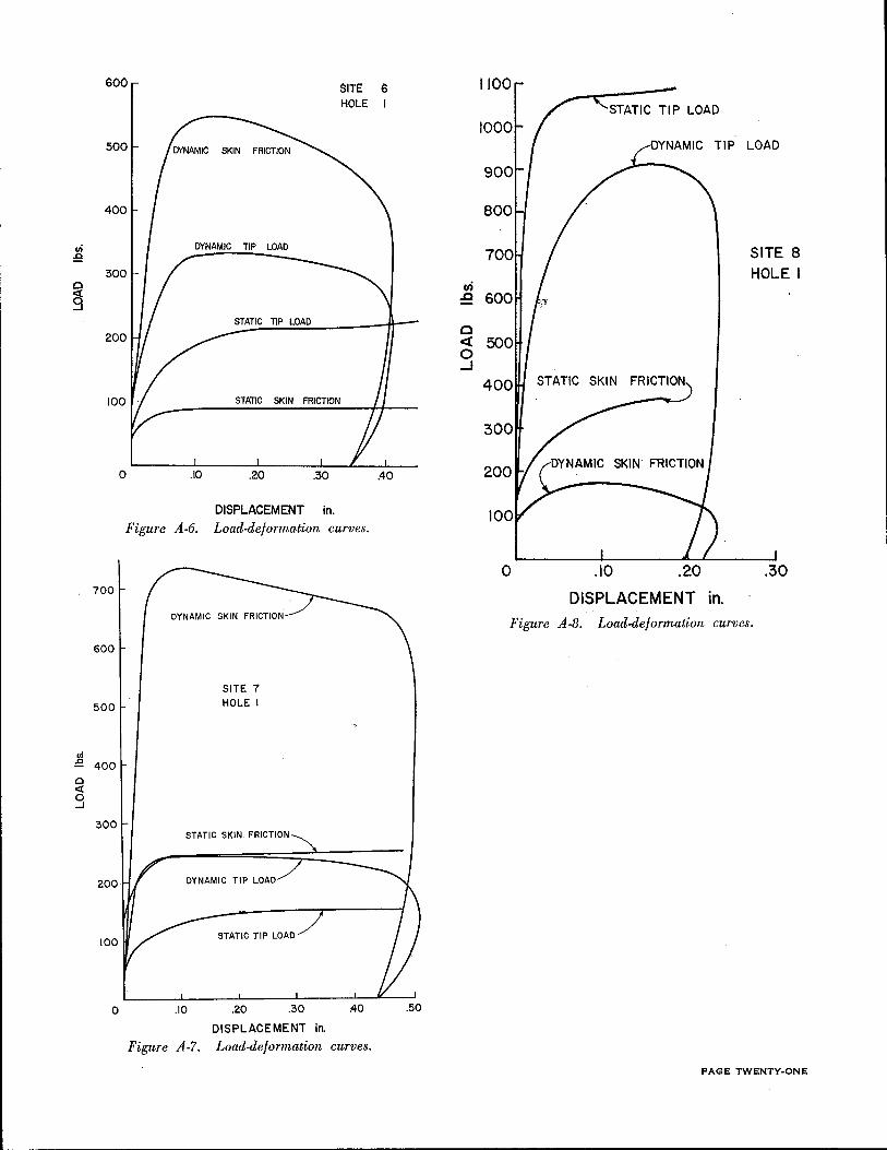
The load-deformation relationships for soil behavior recommended by Smith (8) have been discussed in detail in Chapter I (see Figure 2). Figures A-l through A-12 are static and dynamic load-deformation curves from the tests run in this study. There is one typical set of curves from each test site. A comparison can be made between

800

6 in. DROP

7001

I I

5oo 1 STATIC SKIN FRICTION

ui :e 400

0 <(

g

300

200 SITE HOLE

100

0 .10 .20 .30 .40

DISPLACEMENT in.

Figure A-1. Load-deformation curves.

these curves and Smith's assumed load-deformation curves for soil. This comparison will give some insight into the validity of Smith's model.

In all cases, the dynamic curves shown are from the 6-in. drop in Hole l, and the static curves are from the static test in Hole L

700

SITE 2

HOLE I

500

en m ...J

400 0 <( 0 ...J STATIC TIP LOAD

300

STATIC SKIN FRICTION

200

100

0 .10 .20 .30 AO

DISPLACEMENT IN.

Figure A-2. Load-deformation curves.

PAGE NINETEEN

~-~---~~~~~~--~~~~-~~~------

700

600 DYNAMIC SKIN

500

Ill 400 .a

0 <t 0 ..J 300

0 1.0 2.0 DISPLACEMENT

3.0 in

SITE 3

HOLE I

4.0

Figure A-3. Load-deformation curves.

500 DYNAMIC SKIN FRICTION

400 SITE

HOLE

.; 300 :£!

0 <t DYNAMIC TIP lOAD 9 200

100

0

DISPLACEMENT in.

Figure A-4. Load-deformation curves.

PAGE TWENTY

Tooo~ f'\'ov••"" sKIN FRICTioN

STATIC TIP LOAD

500

eli .0

0 400 <( 0 ..J

300

SITE 5

2.00 HOLE

0 .10 .20 .30 AO

DISPLACEMENT in.

Figure A-5. Load-deformation curves. :J:

600 SITE 6 HOLE

500 LOAD

400

ui :e 300

0

9 STATIC TIP LOAD

200

100 STATIC SKIN FRICTION

0 .10 .20 .30 .40

DISPLACEMENT in. Figure A-6. Load-deformation curves.

0 .10 .20 .30 700 DISPLACEMENT in.

Figure A-8. Load-deformation curves.

600

SITE 7

500 HOLE I

cri :9 400 0 <( 0 ...1

300 STATIC SKIN FRICTION

200 DYNAMIC TIP LOAD

STATIC TIP LOAD

0 .10 .20 .30 :40 .50

DISPLACEMENT in.

Figure A-7. Load-deformation curves.

PAGE TWENTY-ONE

DYNAMIC TIP LOAD 800

700

600 700

500 SITE 10

600 HOLE I SITE 9

en HOLE I ~ DYNAMIC TIP LOAD 0

400

g DYNAMIC SKIN FRICTION u; 500 .0

300 0 <t 0 ..J 300 200

STATIC SKIN FRICTION

100 200

0 .10 .20 .30

DISPLACEMENT in.

Figure A-9. Load-deformation curves. DYNAMIC SKIN FRICTION

.10 .20 .30

DISPLACEMENT in.

Figure A-10. Load-deformation curves.

PAGE TWENTY-TWO

1400

STATIC TIP LOAD

900 1200

~DYNAMIC TIP LOAD 1000.

800 ~ 800

0 LABOflATORY 500 < TEST

0 ..J SATURATED

600 OTTAWA SAND

SITE II

u; 400 HOLE l

400 .c STATIC SKIN

0 FRICTION

~ 20 ....J

300 0

0 .05 .I

DISPLACEMENT in.

200 STATIC SKIN FRICTION Figure A·l2. Load-deformation curves.

100

-DYNAMIC SKIN FRICTION

0 10 20

01 SPLACEMENT in. Figure A-11. Load-deformation curves.

PAGE TWENTY-THREE

APPENDIX B

DATA REDUCTION FROM THE VISICORDER TRACE

The Oscillograph of a Dynamic Test

Several items of data were required from each dy­namic test run. Figure B-1 is a typical oscillograph of a dynamic test.

The maximum dynamic load at the tip of the pile is found at Point A. The maximum dynamic skin fric­tion is found at Point B. The displacement velocity of the pile is obtained by determining the slope of line C-D. The maximum pile displacement is the quantity E. The dynamic soil rebound is quantity F. The pile's perma­nent set is quantity G.

The Static Test The tip load, skin friction, and pile displacement

were recorded during the static tests. With these data, the pile load-settlement curves for the test could be drawn (see Figure B-2). From these curves, the maximum static tip load (A), the maximum static skin friction (B), and the soil's static quake (Qt and Qf) can be determined.

F --;J I I 1\ I I B\ E

G "\ I 1 J I DISPLACE MENT

v i--!-../ / lo~IM FRI CTJON

\ _/ I\._\ ITIPLO D

'o

500

400

IIi ~

0 300 <( 0 ..J

200

100

.10 .20 .30

DISPLACEMENT in.

.40

Figure B-1. Typical oscillograph. Figure B-2. Typical static load-settlement curves.

PAGE TWENTY.,FOUR