i

Dynamic analysis of tapered circular discs made of

isotropic and orthotropic materials using Rayleigh-Ritz

method and ANSYS

Chirag Delvadiya

A thesis

in

the Department

of

Mechanical and Industrial Engineering

Presented in Partial Fulfillment of the Requirements

For the Degree of

Master of Applied Science (Mechanical Engineering) at

Concordia University

Montreal, Quebec, Canada

Sept 30

©Chirag Delvadiya 2016

ii

CONCORDIA UNIVERSITY School of Graduate Studies

This is to certify that the thesis prepared

By: Chirag Kantilal Delvadiya

Entitled: Dynamic analysis of tapered circular discs made of isotropic and

orthotropic materials using Rayleigh-Ritz method and ANSYS

and submitted in partial fulfillment of the requirements for the degree of

Master of Applied Science (Mechanical Engineering)

complies with the regulations of the University and meets the accepted standards with respect to originality and quality.

Signed by the final examining committee:

Dr. W.Ghaly Chair

Dr. J. Dargahi Examiner

Dr. L. Lin Examiner

Dr. R. Ganesan Supervisor

Approved by

Chair of Department or Graduate Program Director

Dean of Faculty

Date November 4, 2016

iii

ABSTRACT

Dynamic analysis of tapered circular discs made of isotropic and orthotropic materials

using Rayleigh-Ritz method and ANSYS

Tapered rotating circular disc provides advantages of preferred stress state compared to

the uniform-thickness circular disc rotating at the same speed. Hence, linearly-tapered circular

disc and circular disc with hyperbolic profile along radial direction, often known as Stodola’s

disc, are increasingly being used in many engineering applications such as in automobiles,

turbomachinery, steam turbines, flywheels, and space structures. It is important to study the in-

plane dynamics and out-of-plane dynamics of such circular discs as they play a vital role in

causing vibration and noise. Design of circular disc for such applications also requires the

knowledge of three-dimensional bending vibration characteristics of the disc. The present

thesis aims at developing a generalized formulation and then to investigate the three-

dimensional in-plane and out-of-plane vibration characteristics of uniform-thickness circular

annular disc, linearly-tapered circular annular disc, and Stodola’s disc with clamped-free

boundary condition.

The trigonometric functions in circumferential coordinate are employed in all the three

displacement components in Rayleigh-Ritz method to calculate the natural frequencies. The

numerical approach based on Rayleigh-Ritz method with finite-element-like modification has

been developed to study the free vibration behaviour of the tapered circular discs made of

isotropic and orthotropic materials and of clamped-free boundary condition. Numerical and

symbolic computations have been performed using MATLAB and MAPLE software. The

results for natural frequencies have been validated using Finite Element Method using ANSYS

and results from previous literature wherever available. A comprehensive parametric study is

conducted to study the effects of various design parameters.

iv

ACKNOWLEDGEMENTS

Firstly, I would like to dedicate this accomplishment to my parents, Mr. Kantilal

Delvadiya and Mrs. Lalitaben Delvadiya. I want thank my brother Hardik for providing

continuous moral support and my fiancée Krishna for her love, care, understanding and

patience. I am blessed because you all love me.

Then, I am grateful to my thesis supervisor Professor Rajamohan Ganesan for his time,

continuous support and valuable guidance provided during my research. I am grateful to

receive the valuable suggestions from my supervisor during thesis writing period. His

perfectionism has self-realized me lifelong learning. I gratefully acknowledge the funding

sources for my research provided by NSERC and Concordia University.

Finally, I am thankful to my friends, Jignesh and Reynaldo, for the time we spent

together.

v

Table of Contents

ABSTRACT ............................................................................................................................. iii

ACKNOWLEDGEMENTS ...................................................................................................... iv

List of Figures ........................................................................................................................... ix

List of Tables ........................................................................................................................... xii

Nomenclature .......................................................................................................................... xiv

Chapter 1 Introduction ............................................................................................................... 1

1.1 General .......................................................................................................................... 1

1.2 Three-dimensional vibration analysis in mechanical design ........................................ 4

1.3 Hamilton’s principle and approximate methods ........................................................... 5

1.3.1 Rayleigh-Ritz method ............................................................................................... 5

1.4 Literature survey ........................................................................................................... 7

1.4.1 Review of vibration analysis of uniform thickness circular discs ............................ 8

1.4.2 Review of vibration analysis of linearly-tapered and non-linearly tapered circular

discs.................................................................................................................................. 10

1.4.3 Review of vibration analysis of rotating circular discs ........................................... 11

1.5 Objective of thesis....................................................................................................... 13

1.6 Layout of thesis ........................................................................................................... 14

Chapter 2 Three-dimensional in-plane and out-of-plane vibrations of annular clamped-free

disc of uniform thickness ......................................................................................................... 16

2.1 Introduction ................................................................................................................. 16

2.2 Modelling .................................................................................................................... 17

vi

2.2.1 Formulation for strain energy ................................................................................. 17

2.2.2 Formulation for kinetic energy ............................................................................... 20

2.3 Solution by Rayleigh-Ritz method.............................................................................. 21

2.3.1 Maximum Strain energy ......................................................................................... 24

2.3.2 Maximum kinetic energy ........................................................................................ 25

2.3.3 Rayleigh’s quotient ................................................................................................. 25

2.3.4 Formulation of eigenvalue problem ........................................................................ 27

2.4 Results and Discussion ............................................................................................... 28

2.4.1 Pure circumferential mode and pure transverse mode ............................................ 29

2.4.2 Coupled mode shapes ............................................................................................. 30

2.5 Example ...................................................................................................................... 31

2.6 Rayleigh’s damping .................................................................................................... 45

2.7 Formulation for Orthotropic disc ................................................................................ 49

2.7.1 Modelling strain energy and kinetic energy ............................................................ 49

2.7.2 In-plane and out-of-plane vibration analysis of orthotropic disc ............................ 51

2.8 Parametric study.......................................................................................................... 54

2.9 Conclusion .................................................................................................................. 57

Chapter 3 Three-dimensional in-plane and out-of-plane vibrations of linearly-tapered

clamped-free disc ..................................................................................................................... 59

3.1 Introduction ................................................................................................................. 59

3.2 Modelling .................................................................................................................... 61

3.2.1 Maximum strain energy and maximum kinetic energy .......................................... 63

vii

3.3 Rayleigh-Ritz solution ................................................................................................ 66

3.3.1 Eigenvalue problem for in-plane vibrations ........................................................... 66

3.3.2 Eigenvalue problem for out-of-plane vibrations ..................................................... 67

3.4 Parametric study on isotropic disc .............................................................................. 68

3.4.1 In-plane vibrations of linearly-tapered isotropic disc ............................................. 68

3.4.2 Out-of-plane vibrations of linearly-tapered isotropic disc ...................................... 70

3.5 Vibration analysis of linearly-tapered orthotropic disc .............................................. 71

3.5.1 In-plane vibrations of linearly-tapered orthotropic disc ......................................... 72

3.5.2 Transverse vibrations of linearly-tapered orthotropic disc ..................................... 73

3.6 Parametric study on orthotropic discs ......................................................................... 74

3.7 Rayleigh’s damping for linearly-tapered disc ............................................................. 80

3.8 Conclusion .................................................................................................................. 83

Chapter 4 Three-dimensional in-plane and out-of-plane vibrations of non-linearly tapered

clamped-free disc ..................................................................................................................... 85

4.1 Introduction ................................................................................................................. 85

4.2 Modelling .................................................................................................................... 85

4.3 Parametric study on isotropic Stodola’s discs ............................................................ 88

4.4 Parametric study on orthotropic Stodola’s discs ......................................................... 90

4.5 Rayleigh’s damping for Stodola’s disc ....................................................................... 91

4.6 Conclusion .................................................................................................................. 94

Chapter 5 Bending mode vibrations of rotating disc of non-linear thickness variation .......... 95

5.1 Introduction ................................................................................................................. 95

viii

5.2 Modelling .................................................................................................................... 96

5.3 Equations of motion .................................................................................................. 101

5.4 Bending mode vibrations of rotating Stodola’s disc ................................................. 105

5.4.1 Maximum strain energy and maximum kinetic energy for bending mode ........... 106

5.4.2 Solution using Rayleigh-Ritz method ................................................................... 107

5.4.3 Solution using Finite element method (using ANSYS) ........................................ 108

5.4.4 Example ................................................................................................................ 109

5.5 Parametric study........................................................................................................ 110

5.5.1 Effect of rotational speed on lowest bending mode natural frequency ................. 110

5.5.2 Effect of taper parameter on the lowest bending mode natural frequency ........... 113

5.5.3 Effect of degree of orthotropy on natural frequency ............................................ 114

5.6 Conclusion ................................................................................................................... 116

Chapter 6 Conclusion and future work .................................................................................. 117

6.1 Major Contributions ..................................................................................................... 117

6.2 Conclusions .................................................................................................................. 118

6.3 Future recommendations .............................................................................................. 120

Appendix A ............................................................................................................................ 121

Appendix B ............................................................................................................................ 124

Appendix C ............................................................................................................................ 127

Bibliography .......................................................................................................................... 129

ix

List of Figures

Figure 1.1: Application of non-linearly tapered circular disc in turbomachinery [3] ............... 3

Figure 1.2: Application of uniform thickness circular disc in automobile [4] .......................... 3

Figure 2.1: Geometry and coordinate system for uniform-thickness disc .............................. 31

Figure 2.2 : SOLID186 homogeneous structural solid element geometry [41] ...................... 33

Figure 2.3: SHELL 281 element geometry [41] ..................................................................... 34

Figure 2.4: Comparison of transverse deformations in the lowest out-of-plane mode obtained

using ANSYS and second-degree polynomial ................................................................. 36

Figure 2.5: Comparison of transverse deformations in the lowest out-of-plane mode obtained

using ANSYS and third-degree polynomial .................................................................... 37

Figure 2.6: Comparison of transverse deformations in the lowest out-of-plane mode obtained

using ANSYS and fourth-degree polynomial .................................................................. 38

Figure 2.7: Comparison of radial deformations in the lowest out-of-plane mode obtained

using ANSYS and second-degree polynomial ................................................................. 40

Figure 2.8: Comparison of radial deformations in the lowest out-of-plane mode obtained

using ANSYS and third-degree polynomial .................................................................... 40

Figure 2.9: Comparison of radial deformations in the lowest out-of-plane mode obtained

using ANSYS and fourth-degree polynomial .................................................................. 41

Figure 2.10: Comparison of radial deformations in the lowest out-of-plane mode obtained

using ANSYS and fifth-degree polynomial ..................................................................... 41

Figure 2.11: Comparison of radial deformations in the lowest out-of-plane mode obtained

using ANSYS and sixth-degree polynomial .................................................................... 42

Figure 2.12: The 𝑛 = 0 bending mode vibration and circumferential mode vibration........... 44

Figure 2.13:The 𝑛 = 1 mode vibration and 𝑛 = 2 mode vibration ....................................... 44

Figure 2.14: The 𝑛 = 3 mode vibration and 𝑛 = 4 mode vibration ...................................... 44

x

Figure 2.15: Variation of damping ratio with circular natural frequency ............................... 48

Figure 2.16: Geometry of SHELL 181 [41] ............................................................................ 53

Figure 3.1: CAD geometry of turbofan of GEnx .................................................................... 60

Figure 3.2: Cross-sectional geometry and coordinate system of linearly-tapered disc .......... 63

Figure 3.3: Variation of the lowest in-plane mode frequency with outer thickness and radius

ratio .................................................................................................................................. 69

Figure 3.4: Variation of the lowest in-plane mode frequency with taper angle of linearly-

tapered isotropic disc for beta value of 0.3 ...................................................................... 70

Figure 3.5: Variation of the lowest transverse mode frequency with taper angle of linearly-

tapered isotropic disc for beta value of 0.25 .................................................................... 70

Figure 3.6: Variation of the lowest transverse mode frequency with linear taper and radius

ratio .................................................................................................................................. 71

Figure 3.7: The lowest bending and the lowest circumferential mode vibrations of linearly-

tapered disc made of Graphite-Polymer composite material having beta value of 0.2 ... 75

Figure 3.8: Variation of the lowest in-plane mode natural frequency of linearly-tapered

orthotropic disc with respect to linear-taper and radius ratio .......................................... 76

Figure 3.9: Behaviour of orthotropic disc in in-plane vibration mode with respect to taper

angle and radius ratio ....................................................................................................... 77

Figure 3.10: Variation of damping ratio with circular natural frequency of linearly-tapered

isotropic disc .................................................................................................................... 82

Figure 4.1: Cross-sectional geometry and coordinate system for Stodola’s disc ................... 86

Figure 4.2: Variation of damping ratio with circular natural frequency of isotropic Stodola’s

disc ................................................................................................................................... 93

Figure 5.1: Variation of natural frequency 𝑓3 of Stodola’s disc with taper parameter and

rotational speed for beta value of 0.2 ............................................................................. 113

xi

Figure 5.2: Variation of frequency parameter with the degree of orthotropy for Stodola’s disc

of beta value of 0.2 and 𝑣21 = 0.3 ................................................................................ 115

xii

List of Tables

Table 2.1: Lowest non-dimensional frequencies grouped according to corresponding mode

shapes ............................................................................................................................... 32

Table 2.2: Transverse displacement values for different radial coordinate values in the lowest

out-of-plane mode ............................................................................................................ 35

Table 2.3: Radial deformation values for circumferential coordinate values in the lowest out-

of-plane mode .................................................................................................................. 39

Table 2.4: Comparison of Rayleigh-Ritz solution with ANSYS solution .............................. 43

Table 2.5: Estimation of Rayleigh's damping coefficients ...................................................... 47

Table 2.6: Material properties of the orthotropic disc [43] ..................................................... 52

Table 2.7: Comparison of natural frequencies for the orthotropic disc .................................. 53

Table 2.8: Variation of non-dimensional frequency parameter with thickness of the disc ..... 54

Table 2.9: Effect of thickness on in-plane and out-of-plane natural frequencies of

Graphite-Polymer composite disc .................................................................................... 55

Table 2.10: Variation of non-dimensional frequency parameter with Poisson’s ratio of the

circular clamped-free disc of uniform thickness .............................................................. 56

Table 3.1: Variation of natural frequency of the lowest transverse mode with outer thickness

of linearly-tapered orthotropic disc for beta value of 0.2 ................................................ 78

Table 3.2: Variation of natural frequency of lowest transverse mode with outer thickness of

linearly-tapered orthotropic disc for beta value of 0.25 ................................................... 79

Table 3.3: Variation of natural frequency of the lowest transverse mode with outer thickness

of linearly-tapered orthotropic disc for beta value of 0.3 ................................................ 79

Table 3.4: Effect of taper angle on natural frequency of lowest transverse mode of linearly-

tapered orthotropic disc for beta values of 0.2, 0.25 and 0.3 ........................................... 80

xiii

Table 3.5: Estimation of Rayleigh’s damping coefficients for linearly-tapered isotropic disc

.......................................................................................................................................... 81

Table 4.1: Variation of natural frequency of the lowest in-plane mode with taper parameter

of Stodola’s disc for beta value of 0.2 ............................................................................. 88

Table 4.2: Variation of natural frequency of the lowest bending mode with taper parameter of

Stodola’s disc for beta value of 0.2 .................................................................................. 89

Table 4.3: Variation of natural frequency of lowest in-plane mode with taper parameter of

orthotropic Stodola’s disc for beta values of 0.2, 0.25 and 0.3 ........................................ 90

Table 4.4: Estimation of Rayleigh’s damping coefficients for isotropic Stodola’s disc ......... 92

Table 5.1: Comparison of lowest transverse mode natural frequency of Stodola’s disc

rotating at constant angular velocity of 100 rad/sec and beta value of 0.2 .................... 109

Table 5.2: Variation of bending mode natural frequency with rotational speed for the

isotropic Stodola’s disc having radius ratio of 0.2 ......................................................... 110

Table 5.3: Variation of bending mode natural frequency with rotational speed for the

orthotropic Stodola’s disc having radius ratio of 0.2 ..................................................... 112

Table B. 1: Comparison of natural frequencies of uniform-thickness annular C-F disc…...124

Table B. 2: Comparison of natural frequencies of linearly-tapered annular C-F disc……...126

Table C. 1: Selection of number of divisions to calculate the natural frequencies of linearly-

tapered disc….................................................................................................................127

Table C. 2: Selection of number of divisions to calculate the natural frequencies of Stodola’s

disc……………………………………………………………………………………128

xiv

Nomenclature

Symbol Description

Π Total strain energy of disc

𝑇 Total kinetic energy of disc

Π𝑚𝑎𝑥 Maximum strain energy of uniform thickness disc

𝑇𝑚𝑎𝑥 Maximum kinetic energy of uniform thickness disc

ζ Non-dimensional radius

ξ Non-dimensional thickness

𝛽 Radius ratio of disc

𝜍 Damping ratio

Ω Non-dimensional frequency parameter of disc

Ω𝐿𝑇 Frequency parameter of linearly-tapered disc

Ω𝐿𝑇𝑜 Frequency parameter of linearly-tapered orthotropic disc

𝜔 Circular natural frequency of disc

𝛼 Mass-proportional damping coefficient

𝛽𝑘 Stiffness-proportional damping coefficient

𝑎 Ratio of outer radius to thickness

𝐴𝑖𝑗 , 𝐵𝑘𝑙, 𝐶𝑝𝑞 Constant coefficients in assumed displacement polynomials in

in 𝑟, 𝜃 and 𝑧 directions respectively

xv

𝑢𝑟 , 𝑢𝜃 , 𝑢𝑧 Displacements in 𝑟, 𝜃 and 𝑧 directions respectively

𝑈, 𝑉,𝑊 Amplitudes of deformation in 𝑟, 𝜃 and 𝑧 directions respectively

𝑛 Nodal diameter number

𝐶𝑖𝑗 Elements of stiffness matrix

𝑐𝑐 Critical damping

𝑅𝑖 Inner radius of disc

𝑅𝑜 Outer radius of disc

𝐸 Modulus of elasticity

𝐺 Modulus of rigidity

𝑛𝑟 , 𝑛𝜃 , 𝑛𝑧 Constraint functions in 𝑟, 𝜃 and 𝑧 directions respectively

𝑁 Numerator of equation of Rayleigh’s quotient

𝐷 Denominator of equation of Rayleigh’s quotient

𝐸1 Modulus of elasticity in radial direction

𝐸2 Modulus of elasticity in circumferential direction

𝐺12 In-plane shear modulus

𝜌 Density of isotropic material

𝜌𝑜 Density of orthotropic material

𝑣12 Major Poisson’s ratio

𝑣21 Minor Poisson’s ratio

xvi

𝐼, 𝐽 Upper limit of polynomial of radial direction

𝐾, 𝐿 Upper limit of polynomial of circumferential direction

𝑃, 𝑄 Upper limit of polynomial of transverse direction

(Π𝑚𝑎𝑥)𝐿𝑇 Maximum strain energy of linearly tapered disc

(T𝑚𝑎𝑥)𝐿𝑇 Maximum kinetic energy of linearly tapered disc

ℎ𝑚𝑖𝑑 Mid-point thickness of tapered disc

ℎ𝑜 Outer thickness of tapered disc

ℎ𝑖 Inner thickness of tapered disc

𝑠 Taper parameter of Stodola’s disc

(Π)𝑟𝑜𝑡 Strain energy of rotating Stodola’s disc

(T)𝑟𝑜𝑡 Kinetic energy of rotating Stodola’s disc

�� Degree of orthotropy

1

Chapter 1

Introduction

1.1 General

Rotating and non-rotating circular discs of uniform thickness and/or with linear

and non-linear thickness variations have many engineering applications such as

automobiles, turbomachinery, planetary gear box, steam turbines, flywheels, space

structures, etc. Moreover, in some of the applications, the circular discs of non-linear

thickness variations provide certain advantages compared to the uniform thickness or

linearly-tapered profiles. The rotating discs of non-linear thickness variations are well

studied in terms of the stresses generated due to rotational effect and proved to be

advantageous compared to the stressed state of rotating discs of uniform thickness.

Modal analysis of any structural component is performed in order to determine

the natural frequencies and associated mode shapes at the design stage. Moreover, the

modal analysis provides the basis for further detailed dynamic analysis such as transient

analysis, harmonic analysis, etc. For designing the circular disc for specified

application, knowledge of in-plane mode vibrations and out-of-plane mode vibrations

is essential.

In the automotive application of thick circular disc as a disk brake, it is observed

that sound radiates from disc effectively when the disc is vibrating at lowest bending

mode natural frequency [1]. Hence, it is important to study the bending mode vibration.

Moreover, frictional stresses over the disc serve as external forces and excite in-plane,

out-of-plane and coupled modes of vibrations. Due to the friction between rotor and

braking pads, the upper surface of the rotor (i.e. circular disc) wears out with the passage

2

of time due to friction between them, which indeed depends on the material capabilities

of the rotor (i.e. wear resistance and heat resistance). As a result, slight taper is observed

at the top rotor side, which can be dealt as tapered circular disc and as a consequence

dynamic response of the same is changed (in most cases, natural frequency of the

structure is increased because of the taper), which disturbs the initially investigated

design parameters of the uniform thickness rotor and results in higher vibration of car

at higher speed. This is the reason behind the to-and-fro motion of an old car when one

applies the brake or one drives it at higher speed. Hence, out-of-plane vibration

response of the thick tapered circular clamped-free disc with respect to rotational speed

should be studied well in advance in order to increase the robustness in design. In any

application, if this aspect isn’t studied properly, severe vibrations occur which result in

the fatigue failure. Therefore, studying the dynamic behaviour of the thick discs is one

of the major research interests of the researchers.

Consider the application of the thick circular disc in railway wheels, where the

lowest in-plane mode and the lowest out-of-plane mode vibrations are to be studied at

the preliminary design stage. Although there are many factors responsible for the noise

generation during operation of rail-wheel, a significant reduction in the noise can be

achieved by minimizing bending mode vibration frequency of the disc [2] (if the rail-

wheel is modelled as circular tapered clamped-free disc).

The following Figures 1.1 and 1.2 show the application of circular discs of

clamped-free boundary condition in turbomachinery and automobile.

3

Figure 1.1: Application of non-linearly tapered circular disc in turbomachinery [3]

Figure 1.2: Application of uniform thickness circular disc in automobile [4]

4

1.2 Three-dimensional vibration analysis in mechanical design

In actual practice, the critical structural components used for various industrial

applications may be modelled as specific structural elements such as bar, rod, beam,

plate or shell, based on their size/shape characteristics. Researchers have developed

various theories with suitable initial assumptions to study the dynamic behaviour of

such structural elements. For the realistic dynamic analysis of certain problems like

thick beams, thick pressure vessels, thick circular discs in turbomachinery or in

automotive applications, one should go for three-dimensional analysis. Further, the

advantage of developing three-dimensional elasticity problem is that it can be applied

to any structural element irrespective of the size/shape of the structural element.

Furthermore, in many cases, the exact or closed-form solutions to such problems

are not available. Nowadays, modern three-dimensional finite element solutions are

available but to achieve accurate results they can’t justify the time and computational

costs involved in the project. Therefore, researchers always seek accurate and efficient

three-dimensional Rayleigh-Ritz approximate solutions or two-dimensional

approximate solutions based on the criticality of the problem. In the three-dimensional

dynamic analysis, there are no kinematic constraints imposed upon the displacements

of middle surface unlike the case of classical one-dimensional or two-dimensional plate

theories. To solve such three-dimensional elasticity problem, various approximate

methods are widely used which are discussed in the following Section 1.3.

It is possible to solve the structural dynamics problem with the breakdown of the

assemblies and subassemblies partially and applying the structural dynamic analysis

and testing procedures. Modal analysis is one of them and of course the root of all the

advanced dynamic analysis procedures. Modal analysis can be performed with the

5

analytical techniques or experimental techniques. By carrying out analysis, we describe

the structure in terms of its natural characteristics such as natural frequencies and

associated mode shapes and damping.

1.3 Hamilton’s principle and approximate methods

In many cases, it is cumbersome to describe the physical system by applying

Newton’s law, especially when the forces acting on the system are uncertain. Trying to

describe such a system in terms of Newton’s equations of motion requires the

estimation of the total force, which does not seem feasible always. In such cases, the

system can be easily described by equations of motion derived by applying Hamilton’s

principle.

Hamilton’s principle can be stated as follows:

𝛿 ∫ 𝐿 𝑑𝑡 = 0𝑡2

𝑡1

(1.1)

where 𝐿 = 𝑇 − 𝑊 is the Lagrangian function. Here, 𝑇 is the kinetic energy of the

system and 𝑊 is the strain energy of the system under consideration. The above integral

is often known as “action integral”. It states that the variation of integral of Lagrangian

from time 𝑡1 to 𝑡2 is zero provided that variations of displacements are zero at 𝑡1 and 𝑡2.

1.3.1 Rayleigh-Ritz method

Walter Ritz has developed the method that is an extension of Rayleigh’s method,

known as Rayleigh-Ritz method. It provides a better approximation for the fundamental

natural frequency. To use this method, it is necessary to represent the deformed shape

of the structure by series of shape functions multiplied by the constant coefficients. We

know that by taking a finite number of terms in a polynomial, we impose a certain

limitation on the possible shapes of the deflection of the structure. Therefore, the

6

frequencies calculated using a finite number of terms in Rayleigh-Ritz polynomial often

overestimate the values of natural frequencies compared to their exact solutions.

Let Φ1(𝑥),Φ2(𝑥), .. be a series of functions Φ𝑗(𝑥) that suitably represent X, the

deformed shape of the structure under consideration and also satisfy the boundary

conditions. Then we have,

𝑋 = a1Φ1(𝑥) + a2Φ2(𝑥) + ⋯+ a𝑗Φ𝑗(𝑥) (1.2)

where, a1, a2.. are constant coefficients.

From the principle of conservation of energy, Rayleigh’s quotient can be derived as

follows:

𝜔2 =𝑈𝑚𝑎𝑥

𝑇𝑚𝑎𝑥∗

(1.3)

Here, maximum kinetic energy is expressed as 𝜔2𝑇𝑚𝑎𝑥∗ . The accuracy of results also

depends on the selection of the polynomial i.e. how good the polynomial represents the

deformed shape of vibrating body.

In order to have the approximation as close as possible to the exact value, Ritz

proposed to choose the coefficients a1, a2.. such that the result of Equation (1.3) be

minimum [5]. Hence, a system of equations are obtained as follows:

𝜕𝜔2

𝜕𝑎𝑗= 0 (1.4)

Upon simplification,

𝜕𝑈𝑚𝑎𝑥

𝜕𝑎𝑗− 𝜔2

𝜕𝑇𝑚𝑎𝑥∗

𝜕𝑎𝑗= 0 (1.5)

The number of such equations will be the number of coefficients in Equation (1.2). This

system of equation can yield non-zero solution if the determinant of the coefficients of

a1, a2.. is equal to zero. A system of Equation (1.5) can be rewritten as follows:

7

[[𝐾] − 𝜔2[𝑀]][{𝑎𝑗}] = 0 (1.6)

where, [{𝑎𝑗}] = [a1 a2 … ]𝑇 is the column matrix consisting of coefficients. The

determinant of augmented matrix in Equation (1.6) yields the frequency equation and

the roots of this equation represent the circular natural frequencies of vibrations.

1.4 Literature survey

A comprehensive literature review is presented on in-plane and out-of-plane

vibrations of linearly-tapered and non-linearly tapered circular discs. Research work on

vibration analysis of circular discs using Ritz method and finite element method have

been chronicled. The majority of work done in the past is limited to the vibration

analysis of linearly-tapered disc and the non-linearly tapered disc of parabolic profiles

(i.e. convex shape profiles) considering Classical plate theory or Mindlin plate theory.

At the end of this section, the research work conducted on vibration analysis of

rotating discs is presented. From that, it can be concluded that the work on the

transverse vibration of rotating disc with hyperbolic thickness variation is very rare or

limited. The following is the up to date survey categorized based on the subject:

8

1.4.1 Review of vibration analysis of uniform thickness circular discs

At first, vibration problem of a circular disc of free-free boundary conditions was

tackled by Love [6] who derived the equations of motion from the concepts of elasticity

and provided the general solutions. Deresiewicz and Mindlin [7] studied the axially

symmetric transverse vibrations of a circular disc. The frequency responses for the

circular disc of free-free boundary condition obtained using both the classical thin plate

theory and the Mindlin plate theory were presented.

Venkatesan and Kunukkasseril [8] studied the free vibration response of layered

circular plates using shear deformation theory. Guruswamy and Yang [9] developed an

element of 24 DOFs (Degrees Of Freedom) to study the static and dynamic behaviour

of thick circular plates. Irie et al. [10] conducted free vibration analysis based on the

Mindlin plate theory considering nine different boundary conditions. Liew et al. [11]

studied the free flexural vibration of circular and annular Mindlin plates using

Rayleigh-Ritz method. So and Leissa [12] have proposed the three-dimensional

Rayleigh-Ritz solution to study the three-dimensional in-plane and out-of-plane

vibration response of thick circular annular plates. They used the admissible functions

in all three directions by employing trigonometric function in circumferential

coordinate and algebraic polynomials in radial and axial coordinates. The scope of their

formulation was limited to the thick circular discs made of isotropic materials. Kang

[13] applied this three-dimensional Ritz solution to conduct free vibration analysis of

shallow spherical dome. Zhou et al. [14] developed the three-dimensional solution for

circular and annular plates using the Chebyshev-Ritz method. Park [15] introduced 2D

exact solution for in-plane vibration of a clamped circular plate. He used Helmholtz

decomposition to derive uncoupled equations of motion from highly coupled equations

of motion, which were obtained by applying Hamilton’s principle. Recently, Bashmal

9

et al. [16] used the boundary characteristic orthogonal polynomials in the Rayleigh-Ritz

method to obtain the frequency parameters of the annular disc with point elastic

support. Moreover, Bashmal et al. [17] also conducted in-plane free vibration of circular

annular disks considering characteristic orthogonal polynomials in Rayleigh-Ritz

method. The material properties considered in their model were isotropic. Huang and

Chen [18] estimated natural frequency of circular discs with V-notches using Ritz

method. Sridhar and Rao [19] developed a four noded 48 DOF sector element to

conduct large deformation Finite Element Analysis of laminated circular composite

plates. They employed Newton-Raphson method as the nonlinear solution technique.

Recently, Gupta et al [20] studied dynamic behaviour of fiber reinforced composite

discs considering SHELL 181 element using ANSYS. Wang et al. [21] have developed

modified Fourier-Ritz approach to study free in-plane vibration of orthotropic annular

plates with general boundary conditions. They studied the effect of different fiber

reinforcement configurations and rotational speed on natural frequency.

Kim and Dickinson [22] studied flexural vibration of thin, flat annular circular

plates using Rayleigh-Ritz method. They have used a series comprising of orthogonally

generated polynomial functions in Rayleigh-Ritz method. Comparison is made between

natural frequency results obtained using three-dimensional Rayleigh-Ritz approach

(presented in Chapter-2) with results obtained by Kim and Dickinson [22]. This

validation is presented in Appendix B.

10

1.4.2 Review of vibration analysis of linearly-tapered and non-linearly tapered

circular discs

The effect of taper on the dynamic behaviour of the circular disc is an important

parameter to investigate. Early works on analysing the effect of taper were that of

Chandrika Prasad et al. [23] and Gupta and Lal [24], who conducted a dynamic analysis

of linearly-tapered circular discs and parabolically-tapered circular discs respectively.

Soni and Amba Rao’s [25] paper contains the analysis for free axisymmetric

vibrations of orthotropic circular plates of linear thickness variation. Their study

doesn’t account for the non-linear thickness variation. Kirkhope and Wilson [26] have

used the annular finite element method to study the stress and vibration behaviour of

thin rotating discs. Moreover, their element allows the specific thickness variation in

the radius direction. They presented numerical data for free vibration response of

linearly-tapered circular discs and parabolically-tapered circular discs. Mota and Petyt

[27] developed the semi-analytical finite element based on Mindlin theory for the

dynamic analysis of circular disc of varying thickness in the radial direction. Their

formulation was limited to the discs made of isotropic materials.

Lenox and Conway [28] developed an exact, closed-form solution for transverse

vibrations of a thin plate having a parabolic thickness variation. Their proposed solution

involves only the power of radius and constant coefficients which are way simpler than

that for the case of uniform thickness solution with the involvement of Bessel functions.

Reddy and Huang [29] presented the finite element formulation for the non-linear

axisymmetric bending of annular plates considering Reissner-Mindlin plate theory and

Von Karman non-linearity. Singh and Saxena [30] used the Rayleigh-Ritz method to

study the axisymmetric transverse vibration of a circular plate of linear thickness

11

variation and made of isotropic materials. In their study, radial direction deformation is

not accounted in axisymmetric transverse vibration analysis unlike the three-

dimensional formulation presented in this thesis.

Recently, Duan et al. [31] introduced the transformation of variables to translate

the governing equation for the free vibration of the thin annular plate into a fourth-order

generalized hypergeometric equation. Gupta et al. [32] employed the differential

quadrature method to analyse the free vibration response of non-linearly tapered

isotropic discs considering classical plate theory assumption. Vishwanathan and Sheen

[33] used the point collocation method to study free vibration of a circular plate of

variable thickness.

To validate the results of linearly-tapered disc of clamped-free boundary

condition, natural frequencies of linearly-tapered disc of small taper angle are

calculated and compared with that of uniform-thickness circular disc with comparable

thickness. This comparison is given in Appendix B.

1.4.3 Review of vibration analysis of rotating circular discs

The above literature survey is limited to the free vibration analysis of non-rotating

circular discs. The modelling of such discs with the inclusion of rotational effects makes

the problem more relevant to their actual applications. In that case, a problem of rotating

disc involves the gyroscopic effect and the centrifugal forces generated due to the

rotation.

At first, Lamb and Southwell [34] tackled the problem of spinning disc of uniform

thickness using Rayleigh’s method. Nowinski [35] conducted the non-linear transverse

vibration analysis of spinning circular discs rotating at constant angular speed and of

uniform thickness using two-term polynomial in Ritz method. Barasch and Chen [36]

12

have reduced the fourth-order equation of motion to a set of four first-order equations.

They used the modified Adam’s method to study the variation of transverse mode

natural frequency of rotating disc of uniform thickness with rotational speed.

Recently, Baddour [37] derived non-linear equations of motion accounting for the

rotary and in-plane inertia terms for spinning circular disc using Hamilton’s principle

for the first time. She proposed the solution of Helmholtz equations via separation of

variables and further considering the classical Bessel functions. This study was limited

to thin rotating circular disc of uniform thickness. Khoshnood and Jalali [38] conducted

the transverse vibration analysis of rotating orthotropic discs of uniform thickness by

expanding the transverse deformation in Fourier series. Hamidzadeh [39] conducted in-

plane free vibration analysis and stability analysis of rotating annular discs on the basis

of two-dimensional linear plane stress theory of elasticity. He proposed the time

independent solution and time dependent solution of governing equations of motion to

study the influence of rotational speed and radios ratio on the natural frequency of the

disc. Dousti and Jalali [40] calculated the eigenmodes of linearized questions using

collocation method and compared the mode shapes of composite disc and isotropic disc.

The above work is limited to free vibration analysis of the circular rotating discs

of uniform thickness or the linearly-tapered rotating discs.

13

1.5 Objective of thesis

The main objectives of the present study are as follow:

1) To calculate the Rayleigh’s damping coefficients based on modal mass participation

factor to obtain the realistic damping natural frequencies of in-plane mode and out-

of-plane mode vibration of uniform thickness disc, linearly-tapered disc and

Stodola’s disc.

2) To investigate the three-dimensional free vibration response of uniform thickness

circular discs, and linearly-tapered and non-linearly tapered circular discs using

Rayleigh-Ritz method and finite element method using ANSYS.

3) To conduct a comprehensive parametric study to study the effects of taper angles,

taper shapes, radius ratios, material properties, and the degree of orthotropy on free

vibration frequency response of circular disc considering clamped-free boundary

condition.

4) To study the effect of rotational speed on the lowest bending mode natural frequency

of Stodola’s disc considering Kirchhoff hypothesis and linear strain-displacement

relationship. Equations of motion are proposed for a hyperbolic profile for the first

time for further future investigations.

5) The accuracy of proposed Rayleigh-Ritz solutions and Rayleigh-Ritz solutions with

finite-element-like modification is verified by comparing them to finite element

solutions using ANSYS.

14

1.6 Layout of thesis

The present chapter provides a brief introduction, overview of applications and

literature review on free vibrations of uniform thickness and tapered circular discs.

In Chapter 2, the modelling of three-dimensional vibration problem is articulated

considering the theory of elasticity. Then the application of Rayleigh-Ritz method to

free vibration problem of the uniform thickness discs is presented. The selection

procedure is proposed to determine the order of polynomials in Rayleigh-Ritz method.

The procedure for estimation of Rayleigh’s damping coefficients based on modal mass

participation factor is presented. At the end of the Chapter, strain energy and kinetic

energy equations are determined for orthotropic discs. Rayleigh-Ritz solutions are

validated by comparing them with ANSYS solutions.

Chapter 3 contains the proposed analytical approach to investigate the three-

dimensional vibration response of linearly-tapered circular discs which is developed

based on the classical Rayleigh-Ritz method with finite-element-like modification. The

complete mathematical formulation is presented and explained along with the

numerical data of the lowest in-plane and the lowest out-of-plane modes natural

frequencies for the linearly-tapered circular disc. Considering clamped-free boundary

condition, the parametric study is conducted based on taper angles and radius ratios.

In Chapter 4, the analytical method derived in Chapter 3 is re-employed to study

the free vibration behaviour of Stodola’s disc. The parametric study is conducted based

on the taper parameters of the Stodola’s disc.

Chapter 5 is devoted to the bending mode vibrations of Stodala’s disc rotating at

constant speed. The effect of rotation on the lowest bending mode natural frequency of

Stodola’s disc is studied by considering the Kirchhoff’s hypothesis and linear strain-

15

displacement relationship. Here, Rayleigh-Ritz method is employed for the first time

for the rotating Stodola’s discs. Moreover, the parametric study on the effects of

constant rotational speeds and degree of orthotropy on free vibration bending mode

natural frequency is conducted.

Finally, major contributions of the present thesis and recommendations for future

work are presented in Chapter 6.

16

Chapter 2

Three-dimensional in-plane and out-of-plane vibrations of annular

clamped-free disc of uniform thickness

2.1 Introduction

This chapter describes the generalized formulation for in-plane and out-of-plane

vibration analyses of a thick circular disc of clamped-free boundary condition and made

of isotropic or orthotropic material. The clamped-free boundary condition is taken into

consideration since this has a wide range of applications. Rayleigh-Ritz method is

employed to obtain the natural frequencies and mode shapes. To study the free vibration

response of the circular disc of uniform thickness, trigonometric functions are

employed in the circumferential coordinate for all the three displacement components

in Rayleigh-Ritz method. The formulation for the three-dimensional vibration analysis

is first developed for the isotropic disc and then extended for the orthotropic disc. The

material chosen for the isotropic disc is Structural Steel having Young’s modulus of

200 GPa and Poisson’s ratio of 0.3. For the orthotropic disc, Graphite-Polymer

Composite material are considered. The material properties for the Graphite-Polymer

Composite material is given in Table 2.6. Rayleigh-Ritz solutions are compared with

the finite element solutions obtained using ANSYS.

A three-dimensional vibration model can reveal more comprehensive and

accurate vibration characteristics of the circular disc involving both in-plane and out-

of-plane modes and coupling between in-plane and out-of-plane motions. For thick

discs, this coupling between in-plane mode and the out-of-plane mode is strong and this

fact necessitates the requirement for the development of efficient three-dimensional

17

Rayleigh-Ritz solutions. In many applications, it is required to know the in-plane and

the out-of-plane response of the disc at the design stage.

2.2 Modelling

In order to use Rayleigh-Ritz method, expressions for total kinetic energy and

total strain energy must be formulated. Here, kinetic energy and strain energy of the

element of the infinitesimal volume are calculated and later integrated over the entire

volume (non-deformed or initial volume) of the disc to derive the expressions for the

total strain energy and total kinetic energy. This approach holds true for the continuous

systems.

2.2.1 Formulation for strain energy

Strain energy is the energy stored in a body due to deformation. It is difficult to

keep track of the displacements (deformations), which are usually unknown if it is to

be measured with respect to the Eulerian frame of reference. Hence, it is advantageous

to consider the Lagrangian coordinates and they can be employed by fixing a coordinate

frame on the body. The motion of this body-fixed frame indicates the rigid body motion

of the body. Displacements (deformations) measured from this frame of reference

contribute to the strain energy. Hence, it is clear that the strain energy of stationary disc

and rotating disc are the same if they are derived from this approach.

As discussed earlier, consider the infinitesimal volume element of the disc. Strain

energy of such an element can be written as follows:

Π𝑒𝑙𝑒𝑚𝑒𝑛𝑡 =1

2𝜎𝑖𝑗𝜖𝑖𝑗 (2.1)

where, 𝜎𝑖𝑗 and 𝜖𝑖𝑗 are the stress and strain tensors respectively.

18

By integrating the Equation (2.1) over the entire domain of the disc, total strain energy

of the disc can be calculated.

This way total strain energy of the uniform disc is given by:

Π = 1

2∫ ∫ ∫ [𝜎𝑟𝑟 𝜎𝜃𝜃 𝜎𝑧𝑧 𝜎𝑟𝜃 𝜎𝜃𝑧 𝜎𝑧𝑟

𝑅𝑜

𝑅𝑖

2𝜋

0

ℎ2

−ℎ2

]

[ 휀𝑟𝑟

휀𝜃𝜃휀𝑧𝑧

2휀𝑟𝜃

2휀𝜃𝑧

2휀𝑧𝑟]

𝑟𝑑𝑟 𝑑𝜃 𝑑𝑧 (2.2)

where, h is the total thickness of the disc and 𝑅𝑖 and 𝑅𝑜 are the inner radius and the

outer radius of the circular disc respectively. Note that the engineering strains are

considered in Equation (2.2).

Assuming small strains, the stress-strain relations follow the Hooke’s law and

hence the relationship is linear. Again, this doesn’t mean that the deformations in r, θ,

and z directions are small. To derive the expression for strain energy of the disc in

terms of displacements, the first step is to write the stresses in terms of strains and the

strains in terms of displacements. In cylindrical coordinate system, they are as follow:

σrr = λ(εrr + εθθ + εzz) + 2Gεrr (2.3)

σθθ = λ(εrr + εθθ + εzz) + 2Gεθθ (2.4)

σzz = λ(εrr + εθθ + εzz) + 2Gεzz (2.5)

σrθ = 2Gεrθ (2.6)

σθz = 2Gεθz (2.7)

σzr = 2Gεzr (2.8)

εrr =∂ur

∂r (2.9)

19

εθθ =ur

r+

1

r

∂uθ

∂θ (2.10)

εzz =∂uz

∂z (2.11)

εrθ =1

2(1

r

∂ur

∂θ+

∂uθ

∂r−

uθ

r) (2.12)

εzr =1

2(∂ur

∂z+

∂uz

∂r) (2.13)

εθz =1

2(1

r

∂uz

∂θ+

∂uθ

∂z) (2.14)

Substituting Equations (2.3) to (2.14) into Equation (2.2), total strain energy as a

function of displacements (i.e. 𝑢𝑟 , uθ and uz) can be derived. Upon simplification, it

can be written as below:

Π =𝐸

4(1 + 𝑣)∫ ∫ ∫

2𝑣

(1 − 2𝑣)(𝜕𝑢𝑟

𝜕𝑟+

ur

r+

1

𝑟

∂uθ

∂θ+

∂uz

∂z)

𝑅𝑜

𝑅𝑖

2𝜋

0

ℎ2

−ℎ2

2

+ 2(𝜕𝑢𝑟

𝜕𝑟)

2

+ 2(ur

r+

1

𝑟

∂uθ

∂θ)2

+ 2(∂uz

∂z)2

+ (1

r

∂ur

∂θ+

∂uθ

∂r−

uθ

r)2

+ (∂ur

∂z+

∂uz

∂r)2

+ (1

r

∂uz

∂θ+

∂uθ

∂z)2

𝑟𝑑𝑟 𝑑𝜃 𝑑𝑧

(2.15)

In Equation (2.15), E and 𝑣 are the Young’s modulus and Poisson’s ratio of the material

respectively. Moreover, 𝑢𝑟 , uθ and uz are the displacements in 𝑟, θ and z directions

respectively.

To simplify the mathematical calculations, the Equation (2.15) can be reduced to

the non-dimensional form in r and z coordinates by letting ζ and ξ as non-dimensional

parameters respectively.

Let, ζ =𝑟

𝑅𝑜 and ξ =

𝑧

h

20

Recall that h is the total thickness of the disc.

Let’s introduce β as a radius ratio in the lower limit of integration in Equation (2.15).

Rewriting the Equation (2.15) in terms of newly introduced non-dimensional

parameters, one gets:

Π = 𝐸 ℎ

4(1 + 𝑣)∫ ∫ ∫

2𝑣

(1 − 2𝑣)(𝜕𝑢𝑟

𝜕ζ+

ur

ζ+

1

ζ

∂uθ

∂θ+

𝑅𝑜

ℎ

∂uz

∂ξ)

2𝜋

0

1

β

12

−12

2

+ 2(𝜕𝑢𝑟

𝜕ζ)

2

+ 2(ur

ζ+

1

ζ

∂uθ

∂θ)2

+ 2(𝑅𝑜

ℎ

∂uz

∂ξ)2

+ (1

ζ

∂ur

∂θ+

∂uθ

∂ζ−

uθ

ζ)2

+ (𝑅𝑜

ℎ

∂ur

∂ξ+

∂uz

∂ζ)2

+ (1

ζ

∂uz

∂θ+

𝑅𝑜

ℎ

∂uθ

∂ξ)2

ζ𝑑𝜃 𝑑ζ 𝑑ξ

(2.16)

where, β is the radius ratio defined by 𝑅𝑖

𝑅𝑜 . The above Equation (2.16) describes the

strain energy of the disc in terms of displacements 𝑢𝑟 , uθ and uz of an arbitrary point

of the disc.

2.2.2 Formulation for kinetic energy

It is confirmed from the formulation developed in sub-section 2.2.1 that the strain

energy of a stationary disc and that of a rotating disc are the same. It is the kinetic

energy that is not the same and hence the corresponding two vibration models are

different based on the kinetic energy.

The kinetic energy of an infinitesimal volume element of stationary disc is given

by:

𝑇𝑒𝑙𝑒𝑚𝑒𝑛𝑡 = 1

2𝜌𝑣2𝑑𝑉 (2.17)

21

where, 𝜌 is the density of the material and 𝑑𝑉 is the volume of an element. Equation

(2.17) can be re-written as follows:

𝑇𝑒𝑙𝑒𝑚𝑒𝑛𝑡 = 1

2𝜌 [(

𝜕𝑢𝑟

𝜕𝑡)2

+ (𝜕𝑢𝜃

𝜕𝑡)2

+ (𝜕𝑢𝑧

𝜕𝑡)2

] 𝑑𝑉 (2.18)

This kinetic energy of an infinitesimal volume element is integrated over the un-

deformed domain of the disc to determine the total kinetic energy of the non-rotating

disc. This way one gets:

𝑇 = 1

2𝜌ℎ𝑅𝑜

2 ∫ ∫ ∫ [(𝜕𝑢𝑟

𝜕𝑡)2

+ (𝜕𝑢𝜃

𝜕𝑡)2

+ (𝜕𝑢𝑧

𝜕𝑡)2

] 휁𝑑𝜃 𝑑휁 𝑑𝜉2𝜋

0

1

𝛽

12

−12

(2.19)

The above Equation (2.19) describes the total kinetic energy of the disc in terms of

displacements 𝑢𝑟 , uθ and uz of an arbitrary point on the disc.

2.3 Solution by Rayleigh-Ritz method

The equations of motion could have been derived for the uniform thickness disc

by applying Hamilton’s principle. Hamilton’s principle states that the variation of the

integral of the Lagrangian function over time 𝑡1 to 𝑡2 is zero provided that variations of

displacements are zero at time 𝑡1 and 𝑡2. Lagrangian function can be calculated by

assembling strain energy and kinetic energy, which are derived in Section 2.2. Variation

can be performed with respect to each generalized coordinate to generate equations of

motion i.e. to get the first equation of motion, one should perform the variation of

Langrangian function with respect to 𝑢𝑟. For deriving second equation of motion,

perform the variation of Langrangian function with respect to 𝑢𝜃 and so on. This

approach is handy only for the uniform thickness discs but for non-linearly tapered

discs, exact or closed-form solutions for the partial differential equations are not

available.

22

To overcome such difficulty, many approximate methods have drawn the

attention of researchers such as Ritz method, Rayleigh-Ritz method and Galerkin

method and are extensively used to solve the structural dynamic problems. In the

present work, Rayleigh-Ritz method is employed to calculate the approximate natural

frequencies of the uniform-thickness disc.

Rayleigh-Ritz method is the extension of the Ritz’s method. To use this method,

it is necessary to make some assumption of the deflected shape of the vibrating elastic

body. The frequency of vibration will then be found by employing the conservation of

energy principle [5]. In Rayleigh-Ritz method, a number of assumed functions are taken

into consideration to have the closest approximation to the exact solution. Hence, this

method provides not only the lowest approximate frequency but also higher mode

approximate frequencies. The accuracy of this method depends on the choice of

assumed approximation functions that one should select to represent the configuration

of the system during vibration, which also should satisfy the geometric boundary

conditions of structural dynamics problem. It is necessary to find the maximum strain

energy and the maximum kinetic energy of the system in order to derive the Rayleigh’s

quotient, which is the ratio of maximum strain energy to maximum kinetic energy.

Let the displacements in 𝑟, θ and z directions be expressed as the following

assumed sinusoidal variation of vibration response:

𝑢𝑟 = 𝑈 𝑠𝑖𝑛 𝑛𝜃 𝑠𝑖𝑛 𝜔𝑡 (2.20)

𝑢𝜃 = 𝑉 𝑐𝑜𝑠 𝑛𝜃 𝑠𝑖𝑛 𝜔𝑡 (2.21)

𝑢𝑧 = 𝑊 𝑠𝑖𝑛 𝑛𝜃 𝑠𝑖𝑛 𝜔𝑡 (2.22)

where, 𝑛 is the circumferential wave number (i.e. nodal diameter number). It is taken

into consideration in order to distinguish between different mode shapes. Here, 𝑈, 𝑉

23

and 𝑊are the amplitudes of vibration in 𝑟, θ and z directions respectively. 𝜔 is the

circular natural frequency of vibration.

Furthermore, amplitudes U, V and W can be expressed in terms of the

combination of the arbitrary coefficients and algebraic polynomials [12].

𝑈 = 𝑛𝑟 ∑∑ 𝐴𝑖𝑗

𝐽

𝑗=0

𝐼

𝑖=0

ζi ξj (2.23)

𝑉 = 𝑛𝜃 ∑ ∑ 𝐵𝑘𝑙

𝐿

𝑙=0

𝐾

𝑘=0

ζk ξl (2.24)

𝑊 = 𝑛𝑧 ∑ ∑ 𝐶𝑝𝑞

𝑄

𝑞=0

𝑃

𝑝=0

ζp ξq (2.25)

where, 𝑛𝑟 , 𝑛𝜃 𝑎𝑛𝑑 𝑛𝑧 are the constraint functions that depend on geometric boundary

conditions. The functions 𝑛𝑟 , 𝑛𝜃 𝑎𝑛𝑑 𝑛𝑧 are used to impose the necessary boundary

conditions to the model.

Let 𝑛𝑟 = 𝑛𝜃 = 𝑛𝑧 =ζ(ζ−β)

(1−β) for the clamped-free disc.

For example,

At inner edge (𝑟 = 𝑅𝑖), 𝑛𝑟 = 𝑛𝜃 = 𝑛𝑧 = 0. Hence, displacements at inner radius are

restricted to zero.

At outer edge (𝑟 = 𝑅𝑜), 𝑛𝑟 = 𝑛𝜃 = 𝑛𝑧 = 1. Hence, there are no constraints for

displacements at outer radius.

Consider the Equation (2.23). It expresses the amplitude of vibration in 𝑟-direction

which is again the function of combination of arbitrary coefficients, non-dimensional

radius and non-dimensional thickness terms. Here, 𝐼 and 𝐽 indicate the maximum

24

number of non-dimensional radius and thickness terms respectively. For example,

for 𝐼 = 𝐽 = 2, the amplitude in 𝑟 direction consists of 9 terms, which is given by:

𝑈 = 𝑛𝑟 (𝐴22ζ2ξ2 + 𝐴21ζ

2ξ1 + 𝐴12ζ1ξ2 + 𝐴20ζ

2 + 𝐴11ζ1ξ1

+ 𝐴02ξ2 + 𝐴10ζ

1 + 𝐴01ξ1 + 𝐴00)

(2.26)

As a rule of thumb, Equation (2.23) yields (𝐼 + 1)(𝐽 + 1) number of terms for the

specific values of 𝐼 and 𝐽.

2.3.1 Maximum Strain energy

As discussed in earlier Sections, maximum strain energy and maximum kinetic

energy are the building blocks for the Rayleigh’s quotient. After substitution of the

assumed displacements expressed by Equations (2.23), (2.24) and (2.25) into Equation

(2.16), the following maximum strain energy is obtained using MAPLE:

Π𝑚𝑎𝑥 = 𝐸 ℎ

4(1 + 𝑣)∫ ∫ ∫ (

2𝑣

1 − 2𝑣((

𝜕𝑈

𝜕ζ) sin 𝑛𝜃 −

𝑛 𝑉 sin 𝑛𝜃

ζ

2𝜋

0

1

β

12

−12

+ 𝑈 sin 𝑛𝜃

ζ+ 𝑎 (

∂W

∂ξsin 𝑛𝜃)

2

) + 2 (𝜕𝑈

𝜕ζsin 𝑛𝜃)

2

+ 2 (𝑈 sin 𝑛𝜃

ζ−

𝑛 𝑉 sin 𝑛𝜃

ζ)2

+ 2𝑎2 (∂W

∂ξsin 𝑛𝜃)

2

+ (𝑛 𝑈 cos 𝑛𝜃

ζ+

𝜕𝑉

𝜕ζcos 𝑛𝜃 −

𝑉 cos 𝑛𝜃

ζ)2

+ (𝑎∂V

∂ξcos 𝑛𝜃 +

𝑛 𝑊 cos 𝑛𝜃

ζ)2

+ (𝑎∂U

∂ξsin 𝑛𝜃 +

𝜕𝑊

𝜕ζsin 𝑛𝜃)

2

) ζ 𝑑𝜃 𝑑ζ 𝑑ξ

(2.27)

25

In above Equation (2.27), the maximum value of 𝑠𝑖𝑛2 𝜔𝑡 is considered in order to

derive the maximum strain energy.

2.3.2 Maximum kinetic energy

After substitution of the assumed displacements expressed by Equations (2.23),

(2.24) and (2.25) into Equation (2.19), the following total kinetic energy expression is

obtained using MAPLE:

𝑇 =

1

2𝑅𝑜

2ℎ𝜌 𝜔2 ∫ ∫ ∫ (𝑈2 sin2 𝑛𝜃 + 𝑉2 cos2 𝑛𝜃2𝜋

0

1

β

12

−12

+ 𝑊2 sin2 𝑛𝜃) cos2 𝜔𝑡 ζ 𝑑𝜃 𝑑ζ 𝑑ξ

(2.28)

To calculate maximum kinetic energy of the disc, consider the maximum value of

cos2 𝜔𝑡 in the Equation (2.28). This way one gets:

𝑇𝑚𝑎𝑥 =

1

2𝑅𝑜

2ℎ𝜌 𝜔2 ∫ ∫ ∫ (𝑈2 sin2 𝑛𝜃 + 𝑉2 cos2 𝑛𝜃2𝜋

0

1

β

12

−12

+ 𝑊2 sin2 𝑛𝜃) ζ 𝑑𝜃 𝑑ζ 𝑑ξ

(2.29)

Later, complementary displacement functions are used to derive different mode shapes,

which are discussed in the following sub-section 2.4.1. Formulations for maximum

kinetic energy and maximum strain energy hold true for the complementary set of

displacement functions too.

2.3.3 Rayleigh’s quotient

The law of conservation of energy implies that the total energy of the isolated

system is constant. Hence, comparing the maximum kinetic energy and the maximum

strain energy, neglecting damping, Rayleigh’s quotient can be derived as follows:

26

Π𝑚𝑎𝑥 = 𝜔2𝑇∗𝑚𝑎𝑥 (2.30)

where, 𝑇∗𝑚𝑎𝑥 =

1

2 𝜌ℎ𝑅𝑜

2 ∫ ∫ ∫ (𝑈2 sin2 𝑛𝜃 + 𝑉2 cos2 𝑛𝜃 +2𝜋

0

1

β

1

2

−1

2

𝑊2 sin2 𝑛𝜃) ζ 𝑑𝜃 𝑑ζ 𝑑ξ

Therefore,

𝐸ℎ

4(1 + 𝑣)∫ ∫ ∫ (Π𝑢𝑛𝑖 𝑡𝑒𝑟𝑚𝑠) ζ𝑑𝜃 𝑑ζ 𝑑ξ

2𝜋

0

1

β

12

−12

=1

2𝜔2𝜌ℎ𝑅𝑜

2 ∫ ∫ ∫ (𝑇∗𝑢𝑛𝑖

𝑡𝑒𝑟𝑚𝑠) ζ𝑑𝜃 𝑑ζ 𝑑ξ 2𝜋

0

1

β

12

−12

(2.31)

Here,

(Π𝑢𝑛𝑖 𝑡𝑒𝑟𝑚𝑠) =2𝑣

1 − 2𝑣((

𝜕𝑈

𝜕ζ) sin 𝑛𝜃 −

𝑛 𝑉 sin 𝑛𝜃

ζ+

𝑈 sin 𝑛𝜃

ζ

+ 𝑎 (∂W

∂ξsin 𝑛𝜃)

2

) + 2(𝜕𝑈

𝜕ζsin 𝑛𝜃)

2

+ 2(𝑈 sin 𝑛𝜃

ζ−

𝑛 𝑉 sin 𝑛𝜃

ζ)2

+ 2𝑎2 (∂W

∂ξsin 𝑛𝜃)

2

+ (𝑛 𝑈 cos 𝑛𝜃

ζ+

𝜕𝑉

𝜕ζcos 𝑛𝜃 −

𝑉 cos 𝑛𝜃

ζ)

2

+ (𝑎∂V

∂ξcos 𝑛𝜃 +

𝑛 𝑊 cos 𝑛𝜃

ζ)2

+ (𝑎∂U

∂ξsin 𝑛𝜃 +

𝜕𝑊

𝜕ζsin 𝑛𝜃)

2

(2.32)

and

(𝑇∗𝑢𝑛𝑖

𝑡𝑒𝑟𝑚𝑠) = 𝑈2 sin2 𝑛𝜃 + 𝑉2 cos2 𝑛𝜃 + 𝑊2 sin2 𝑛𝜃 (2.33)

27

Hence, Rayleigh’s quotient (Ω2) becomes:

Ω2 =

∫ ∫ ∫ (Π𝑢𝑛𝑖 𝑡𝑒𝑟𝑚𝑠) ζ𝑑𝜃 𝑑ζ 𝑑ξ 2𝜋

0

1

β

12

−12

∫ ∫ ∫ (𝑇∗𝑢𝑛𝑖

𝑡𝑒𝑟𝑚𝑠) ζ𝑑𝜃 𝑑ζ 𝑑ξ 2𝜋

0

1

β

12

−12

=𝑁

𝐷 (2.34)

Note that N and D are the numerator and the denominator of the Rayleigh’s quotient

respectively. In above Equations (2.32), (2.33) and (2.34), subscript ‘𝑢𝑛𝑖’refers to the

vibration model of uniform thickness circular disc.

Upon simplifying the Equations (2.31) and (2.34),

Ω = √2𝜔2𝑅02𝜌(1 + 𝑣)

𝐸 (2.35)

Equation (2.35) represents the non-dimensional frequency parameter of the uniform

disc.

2.3.4 Formulation of eigenvalue problem

To obtain the best possible approximation of natural frequencies for the assumed

shape functions, arbitrary coefficients are adjusted and natural frequency is made

stationary. Minimizing the Rayleigh’s quotient with respect to arbitrary constants

considered in Equations (2.23), (2.24) and (2.25), one gets:

𝜕Ω2

𝜕𝐴𝑖𝑗= 0

(2.36)

𝜕Ω2

𝜕𝐵𝑘𝑙= 0

(2.37)

𝜕Ω2

𝜕𝐶𝑝𝑞= 0

(2.38)

28

These give the set of (𝐼 + 1)(𝐽 + 1) + (𝐾 + 1)(𝐿 + 1) + (𝑃 + 1)(𝑄 + 1) linear

algebraic equations in terms of arbitrary coefficients (i.e. 𝐴𝑖𝑗 , 𝐵𝑘𝑙 𝑎𝑛𝑑 𝐶𝑝𝑞). These

equations are given as follow:

𝜕𝑁

𝜕𝐴𝑖𝑗− Ω2

𝜕𝐷

𝜕𝐴𝑖𝑗= 0 (2.39)

𝜕𝑁

𝜕𝐵𝑘𝑙− Ω2

𝜕𝐷

𝜕𝐵𝑘𝑙= 0 (2.40)

𝜕𝑁

𝜕𝐶𝑝𝑞− Ω2

𝜕𝐷

𝜕𝐶𝑝𝑞= 0 (2.41)

The above equations can be rewritten and represented as the eigenvalue problem,

[[𝐾] − Ω2[𝑀]] [

{𝐴𝑖𝑗}

{𝐵𝑘𝑙}{𝐶𝑝𝑞}

] = 0 (2.42)

where, {𝐴𝑖𝑗}, {𝐵𝑘𝑙} 𝑎𝑛𝑑 {𝐶𝑝𝑞} are column matrices. The dimensions of these matrices

depend on the number of terms considered in Equations (2.23), (2.24) and (2.25).

To have a non-trivial solution, in Equation (2.42) let the determinant of the

augmented matrix be zero. MAPLE code is developed to determine this determinant

and solve for unknowns and, as a result, non-dimensional frequency parameters

(Ω𝑖 , 𝑖 = 1, 2, 3…) are calculated for the assumed nodal diameter numbers.

To study three-dimensional vibrations of the tapered disc, the presented approach

is useful after suitable modifications. For this purpose, the modified Rayleigh-Ritz

procedure is developed and explained in Chapter 3.

2.4 Results and Discussion

It is very clear by now that the number of natural frequencies that can be obtained

from solving the augmented matrix of Equation (2.42) is equal to the number of terms

considered in the assumed shape functions. At this point, it is advisable to conduct

convergence study to determine the exact number of terms to be used in the assumed

29

polynomials, which gives the closest approximation to the exact solution. In Rayleigh-

Ritz method, frequencies should converge to their exact solutions in the upper bound

manner. This study is conducted and explained in the following section.

2.4.1 Pure circumferential mode and pure transverse mode

For the stationary uniform-thickness disc case, the in-plane mode is the pure

circumferential mode, in which there are no radial and transverse deformations present.

If there is no circumferential deformation, the mode shape can be described as a pure

transverse mode. In this formulation, assumed displacement functions and their

complimentary sets are considered to investigate pure transverse mode frequencies and

pure circumferential mode frequencies of the disc.

Assumed set (A):

𝑢𝑟 = 𝑈 𝑐𝑜𝑠 𝑛𝜃 𝑠𝑖𝑛 𝜔𝑡 (2.43)

𝑢𝜃 = 𝑉 𝑠𝑖𝑛 𝑛𝜃 𝑠𝑖𝑛 𝜔𝑡 (2.44)

𝑢𝑧 = 𝑊 𝑐𝑜𝑠 𝑛𝜃 𝑠𝑖𝑛 𝜔𝑡 (2.45)

For 𝑛 = 0, Set (A) describes the lowest transverse mode (i.e. the lowest out-of-plane

mode or the lowest bending mode) and the displacements for this mode are as follows,

𝑢𝑟 = 𝑈 𝑠𝑖𝑛 𝜔𝑡 (2.46)

𝑢𝜃 = 0 (2.47)

𝑢𝑧 = 𝑊 𝑠𝑖𝑛 𝜔𝑡 (2.48)

Complimentary set (B):

𝑢𝑟 = 𝑈 𝑠𝑖𝑛 𝑛𝜃 𝑠𝑖𝑛 𝜔𝑡 (2.49)

𝑢𝜃 = 𝑉 𝑐𝑜𝑠 𝑛𝜃 𝑠𝑖𝑛 𝜔𝑡 (2.50)

𝑢𝑧 = 𝑊 𝑠𝑖𝑛 𝑛𝜃 𝑠𝑖𝑛 𝜔𝑡 (2.51)

30

For 𝑛 = 0, Set (B) yields pure circumferential mode (i.e. the lowest in-plane mode) and

the displacements for this mode are as follows,

𝑢𝑟 = 0 (2.52)

𝑢𝜃 = 𝑉 𝑠𝑖𝑛 𝜔𝑡 (2.53)

𝑢𝑧 = 0 (2.54)

2.4.2 Coupled mode shapes

In the lowest bending mode vibrations, there exist ‘small’ radial deformation and

the transverse component of displacement as the present study is based on a three-

dimensional analysis and is not limited to plane stress or plane strain assumptions.

For 𝑛 ≥ 1, Set (A) functions are considered. Hence, there exist all the three

displacement components and hence named as coupled mode shapes, which can be

identified based on the nodal diameter numbers. If Set (B) functions are chosen to

investigate the coupled mode shapes, it can be inferred that mode shapes may be rotated

by 90 degrees due to the nature of assumed trigonometric functions but they should

have the same frequencies as reported by Set (A).

31

2.5 Example

A uniform thickness disc made of a structural steel material is considered. Let the

inner radius and the outer radius of the disc be 0.4 m and 2 m. The thickness of the disc

is 0.15 m. For the structural steel material, the values of modulus of elasticity and

Poisson’s ratio are 200 GPa and 0.3 respectively.

Figure 2.1: Geometry and coordinate system for uniform-thickness disc

Note that in Rayleigh-Ritz method, if the upper limit of summation is set to

1(which gives four constants coupled with four displacement terms), it generates 12x12

matrix. Just to start with, an equal number of polynomial terms are taken for the ease

of calculations, though these results may not be closest to their exact solutions. These

results are given in the following Table 2.1. Non-dimensional frequency parameters

obtained using MAPLE for 𝐼 = 𝐽 = 𝐾 = 𝐿 = 𝑃 = 𝑄 = 1 are given in the third column.

h

z

𝑅𝑜

𝑅𝑜

𝑅𝑖

𝜃

𝑢𝜃

𝑢𝑧

r

𝑢𝑟

32

Mode set

Non-dimensional frequency

without convergence study

Ω = √2𝜔2𝑅02𝜌(1 + 𝑣)

𝐸

Non-dimensional

frequency

parameter

after convergence

study

Set A

𝑛 = 0

out-of-plane

0.3639

2.6783

3.9915

0.2025

-

-

Set B

𝑛 = 0

in-plane

0.8248

9.0738

46.1847

0.5945

-

-

Set A

𝑛 = 1

coupled

0.3469

1.7524

2.7464

0.1856

-

-

Set A

𝑛 = 2

coupled

0.3526

2.8408

2.9564

0.2406

-

-

Set A

𝑛 = 3

coupled

0.5042

3.3160

-

0.4565

-

-

Set A

𝑛 = 4

coupled

0.8155

3.7955

-

0.7829

-

-

Set A

𝑛 = 5

coupled

1.2383

4.1983

-

1.0818

-

-

Table 2.1: Lowest non-dimensional frequencies grouped according to corresponding

mode shapes

33

In above Table 2.1, frequencies of the lowest in-plane mode, the lowest out-of-

plane mode and the coupled modes for the stated example are demonstrated. For three-

dimensional vibrations of the stationary uniform disc case, the lowest out-of-plane

mode has deformations in transverse as well as in radial directions.

At this point, convergence study is necessary to get the frequencies approximation

closest to the exact frequencies. This can be achieved by the following procedure. Here,

convergence procedure is only explained for the lowest bending mode.

The natural frequencies and mode shapes are calculated for the above-stated example

using ANSYS. In the modal analysis in ANSYS, mode 3 represents pure transverse

mode. In the simulation, SOLID 186 elements are used for the analysis and later results

are compared with that obtained using SHELL 281.

The following Figure 2.2 and Figure 2.3 show the geometry of SOLID 186 and

SHELL 281 elements. The brief descriptions of these elements are given next:

Figure 2.2 : SOLID186 homogeneous structural solid element geometry [41]

SOLID 186 is a higher-order 3-D element that consists of 20 nodes and it exhibits

quadratic displacement behaviour. This element has three degrees of freedom per node

(translations in the nodal X, Y, and Z directions). It supports plasticity, creep, stress

34

stiffening, large deflection and large strain capabilities. The SOLID 186 homogeneous

structural solid element is well suited to modelling irregular meshes that can be

produced by various CAD/CAM systems.

Figure 2.3: SHELL 281 element geometry [41]

The above Figure 2.3 describes the geometry and coordinate system for SHELL 281

element. Furthermore, a triangular-shaped element option is available by defining the

same node number for nodes K, L and O. This element has eight nodes with six degrees

of freedom at each node (three translations in the X, Y and Z axes and rotations about

X, Y and Z axes). SHELL 281 is well suited for analysing thin to moderately thick shell

structures. It is well suited for linear, and large rotation and large strain nonlinear

applications.

Consider the lowest transverse mode. Now it is possible to extract the deformation

values of each point, which are deformed in the transverse direction. Later, these can

be represented as a plot of transverse deformation versus radial coordinate. This

procedure helps to develop more accurate polynomial that can be fed into the above

Rayleigh-Ritz formulation. This results in deriving approximate in-plane and out-of-

plane frequencies which are closer to the exact solutions.

35

A total of 49 points are selected in the radial direction lying on the face of the circular

disc and their respective z-direction deformations are calculated using ANSYS. The

numerical values of transverse deformation are presented in Table 2.2.

26 0.0083 0.00E+00

27 1.6667 0.00E+00

28 0.25 0.00E+00

29 0.3333 0.00E+00

30 0.4166 4.91E-05

31 0.5 3.00E-04

32 0.5833 6.45E-04

33 0.6667 1.10E-03

34 0.75 1.65E-03

35 0.8333 2.28E-03

36 0.9167 2.97E-03

37 1 3.70E-03

38 1.0833 4.47E-03

39 1.1667 5.26E-03

40 1.25 6.07E-03

41 1.3333 6.89E-03

42 1.4167 7.71E-03

43 1.5 8.54E-03

44 1.5833 9.35E-03

45 1.6667 1.02E-02

46 1.75 1.10E-02

47 1.8333 1.18E-02

48 1.9167 1.25E-02

49 2 1.33E-02

Table 2.2: Transverse displacement values for different radial coordinate values in the

lowest out-of-plane mode

It is obvious and clear from Table 2.2 that there is no transverse deformation at the

center of the disc and at the inner radius.

Radial

Coordinate

(m)

Transverse

Displacement

(m)

1 -2 1.33E-02

2 -1.9167 1.25E-02

3 -1.8333 1.17E-02

4 -1.75 1.09E-02

5 -1.6667 1.01E-02

6 -1.5833 9.34E-03

7 -1.5 8.52E-03

8 -1.4167 7.70E-03

9 -1.3333 6.88E-03

10 -1.25 6.06E-03

11 -1.1667 5.25E-03

12 -1.0833 4.46E-03

13 -1 3.70E-03

14 -0.9167 2.96E-03

15 -0.8333 2.28E-03

16 -0.75 1.65E-03

17 -0.6667 1.10E-03

18 -0.5833 6.44E-04

19 -0.5 3.00E-04

20 -0.4166 5.09E-05

21 -0.3333 0.00E+00

22 -0.25 0.00E+00

23 -1.6667 0.00E+00

24 -0.0083 0.00E+00

25 0 0.00E+00

36

The comparison between deformation data of the lowest out-of-plane mode with

different degrees of a polynomial function is given next.

It is clear from the following Figure 2.4 that second-degree polynomial doesn’t

represent accurately the deformation that was obtained using ANSYS. This concludes

the requirement of higher degree polynomial in Rayleigh-Ritz procedure to represent

the actual deformation shape.

Figure 2.4: Comparison of transverse deformations in the lowest out-of-plane mode

obtained using ANSYS and second-degree polynomial

y = 0.0036x2 + 9E-06x - 0.0001

-2.00E-03

0.00E+00

2.00E-03

4.00E-03

6.00E-03

8.00E-03

1.00E-02

1.20E-02

1.40E-02

1.60E-02

-2.5 -2 -1.5 -1 -0.5 0 0.5 1 1.5 2 2.5

Def

orm

atio

n i

n z

-dir

ecti

on (

m)

Radial coordinate (m)

z-direction deformation

in pure transverse mode

ANSYS

37

In the following Figure 2.5, the comparison is made between transverse deformations

in the lowest out-of-plane mode obtained using ANSYS and third-degree polynomial.

Figure 2.5: Comparison of transverse deformations in the lowest out-of-plane mode

obtained using ANSYS and third-degree polynomial

It is concluded from the following Figure 2.6 that 4th-degree polynomial best fits the z-

direction deformation obtained using ANSYS. Both curves coincide in Figure 2.6,

where the 4th-degree polynomial equation is used. It means that to represent the

transverse mode shape, one needs higher degree polynomial terms for W.

In Figure 2.4 to Figure 2.6, the dark dotted line represents the transverse deformation

curve plotted using the transverse deformation data obtained using ANSYS. The light

dotted line represents the curve obtained using the equation with assumed degree of the

polynomial.

y = 3E-06x3 + 0.0036x2 + 2E-06x - 0.0001

-2.00E-03

0.00E+00

2.00E-03

4.00E-03

6.00E-03

8.00E-03

1.00E-02

1.20E-02

1.40E-02

1.60E-02

-2.5 -2 -1.5 -1 -0.5 0 0.5 1 1.5 2 2.5

Def

orm

atio

n i

n z

-dir

ecti

on (

m)

Radial coordinate (m)

z-direction deformation

in pure transverse mode

ANSYS

38

Figure 2.6: Comparison of transverse deformations in the lowest out-of-plane mode

obtained using ANSYS and fourth-degree polynomial

There exists a small radial deformation in the lowest out-of-plane mode, which

should be taken into account in Rayleigh-Ritz procedure. As it is ‘small’ radial

deformation in the lowest out-of-plane mode, a number of deformation points are

considered from ANSYS.

A total of 491 points are selected in the whole circumference of the disc and radial

deformations are noted at each point. These deformations are shown in Table 2.3. In

Table 2.3, the first column indicates the circumferential position of the point and the

second column indicates the respective radial deformation.

y = -0.0003x4 + 3E-06x3 + 0.0046x2 + 2E-06x - 0.0005

-2.00E-03

0.00E+00

2.00E-03

4.00E-03

6.00E-03

8.00E-03

1.00E-02

1.20E-02

1.40E-02

1.60E-02

-2.5 -2 -1.5 -1 -0.5 0 0.5 1 1.5 2 2.5

Def

orm

atio

n i

n z

-dir

ecti

on

(m

)

Radial coordinate (m)

z-direction deformation

in pure transverse mode

ANSYS

39

Circumferential

Coordinate

(m)

Radial

deformation

(m)

470 12.029 0.013274

1 0 0.013274 471 12.055 0.013274

2 2.56E-02 0.013274 472 12.08 0.013274

3 5.12E-02 0.013274 473 12.106 0.013274

4 7.69E-02 0.013274 474 12.131 0.013274

5 0.10253 0.013274 475 12.157 0.013274

6 0.1282 0.013274 476 12.182 0.013274

7 0.15387 0.013274 477 12.207 0.013274

8 0.17953 0.013274 478 12.233 0.013274

9 0.20519 0.013274 479 12.259 0.013274

10 0.23092 0.013274 480 12.285 0.013274

11 0.25665 0.013274 481 12.31 0.013274

12 0.28253 0.013274 482 12.336 0.013274

13 0.30841 0.013274 483 12.362 0.013274

14 0.33406 0.013274 484 12.388 0.013274

15 0.35971 0.013274 485 12.413 0.013274

85 2.1545 0.013277 486 12.439 0.013274

86 2.18 0.013278 487 12.465 0.013274

87 2.2055 0.013278 488 12.49 0.013274

88 2.2312 0.013278 489 12.516 0.013274

89 2.2569 0.013278 490 12.541 0.013274

90 2.2824 0.013278 491 12.566 0.013274

Table 2.3: Radial deformation values for circumferential coordinate values in the

lowest out-of-plane mode

In the following Figure 2.7 to Figure 2.11, the dark dotted line represents the radial

deformation curve in pure transverse mode, plotted using the r-deformation data

obtained using ANSYS. The light dotted line represents the curve represented by the

40

equation with assumed degree of the polynomial.

Figure 2.7: Comparison of radial deformations in the lowest out-of-plane mode

obtained using ANSYS and second-degree polynomial

Figure 2.8: Comparison of radial deformations in the lowest out-of-plane mode

obtained using ANSYS and third-degree polynomial

y = -5E-07x2 + 6E-06x + 0.0133

0.013265

0.013270

0.013275

0.013280

0.013285

0.013290

0.013295

0 2 4 6 8 10 12 14

Def

orm

atio

n i

n r

-dir

ecti

on

(m

)

Circumferential coordinate (m)

r-direction deformation

in pure transverse mode

ANSYS

y = 2E-09x3 - 6E-07x2 + 7E-06x + 0.0133

0.013265

0.013270

0.013275

0.013280

0.013285

0.013290

0.013295

0 2 4 6 8 10 12 14

Def

orm

atio

n i

n r

-dir

ecti

on (

m)

Circumferential coordinate (m)

r-direction deformation

in pure transverse mode

ANSYS

41

Figure 2.9: Comparison of radial deformations in the lowest out-of-plane mode

obtained using ANSYS and fourth-degree polynomial

Figure 2.10: Comparison of radial deformations in the lowest out-of-plane mode

obtained using ANSYS and fifth-degree polynomial

y = 2E-08x4 - 5E-07x3 + 3E-06x2 - 4E-06x + 0.0133

0.013270

0.013275

0.013280

0.013285

0.013290

0.013295

0 2 4 6 8 10 12 14

Def

orm

atio

n i

n r

-dir

ecti

on

(m

)

Circumferential coordinate (m)

r-direction deformation

in pure transverse mode

ANSYS

y = -1E-10x5 + 2E-08x4 - 5E-07x3 + 4E-06x2 - 5E-06x + 0.01330.013272

0.013274

0.013276

0.013278

0.013280

0.013282

0.013284

0.013286

0.013288

0.013290

0.013292

0.013294

0 2 4 6 8 10 12 14

Def

orm

atio

n i

n r

-dir

ecti

on (

m)

Circumferential coordinate (m)

r-direction deformation

in pure transverse mode

ANSYS

42

Figure 2.11: Comparison of radial deformations in the lowest out-of-plane mode

obtained using ANSYS and sixth-degree polynomial

It is interpreted from Figure 2.7 to Figure 2.11 that, a 6th-degree polynomial best fits

the radial deformation graph obtained from the ANSYS. Hence, a higher degree of z-

direction terms is needed in ‘U’ to have a closer approximation of the out-of-plane

mode natural frequency.

The above convergence study is strictly for the lowest out-of-plane mode vibration

analysis. The same methodology can be repeated to study the lowest in-plane mode and

the coupled modes.

Comparison of Rayleigh-Ritz solutions obtained after convergence study is made

with Finite Element solutions for natural frequencies of the lowest in-plane mode, the

lowest out-of-plane mode, and the coupled modes. The comparison is shown in the

following Table 2.4.

y = -4E-10x6 + 2E-08x5 - 2E-07x4 + 1E-06x3 - 1E-06x2 + 1E-06x + 0.0133

0.013270

0.013275

0.013280

0.013285

0.013290

0.013295

0 2 4 6 8 10 12 14

Def

orm

atio

n i

n r

-dir

ecti

on

(m

)

Circumferential coordinate (m)

r-direction deformation

in pure transverse mode

ANSYS

43

Nodal

diameter

number

Degree

of

Polynomial

Size of

augmented

matrix

Rayleigh-Ritz

solution

ANSYS

solution

Non-

dimensional

frequency

Natural

Frequency

(in Hz)

Natural

frequency

(in Hz)

SOLID

186

SHELL

281

𝑛 = 0

bending

mode

𝐽 = 𝑃 = 4

and

𝐼 = 𝑄 = 2

30x30 0.2025 50.44 47.45 46.74

𝑛 = 0

in-plane

mode

𝐾 = 𝐿 = 4 25x25 0.5945 148.09 148.65 148.49

𝑛 = 1

coupled

mode

𝐽 = 𝑃 =

𝐿 = 4

and

𝐼 = 𝐾 =

𝑄 = 2

45x45

0.1856 46.23 43.67 42.08

𝑛 = 2

coupled

mode

0.2406 59.93 57.78 57.05

𝑛 = 3

coupled

mode

0.4565 113.72 112.81 112.39

𝑛 = 4

coupled

mode

0.7829 195.02 193.88 193.39

Table 2.4: Comparison of Rayleigh-Ritz solution with ANSYS solution

Recall that 𝐼, 𝐽, 𝐾, 𝐿, 𝑃 and 𝑄 denote the upper limit of summation in Equations (2.23),

(2.24) and (2.25).

The mode shapes of the uniform thickness disc in the lowest bending mode

vibration, the lowest circumferential mode vibration, and for nodal diameter values of

one, two, three and four are presented in the following Figure 2.12 to Figure 2.14:

44

Figure 2.12: The 𝑛 = 0 bending mode vibration and circumferential mode vibration

Figure 2.13:The 𝑛 = 1 mode vibration and 𝑛 = 2 mode vibration

Figure 2.14: The 𝑛 = 3 mode vibration and 𝑛 = 4 mode vibration

45

2.6 Rayleigh’s damping

Rayleigh’s damping is proportional to a linear combination of mass and stiffness.

The damping matrix can be written as follows:

[𝐶] = 𝛼[𝑀] + 𝛽𝑘[𝐾] (2.55)

One may assume a constant damping ratio for all significant modes. That’s indeed

unrealistic. It is observed that modal mass participation decreases as mode number

increases. From this, it is clear that as mode number increases, frequency increases

according to the formula, 𝜔𝑛 = √𝐾

𝑀 . Considering critical damping formula,

𝑐𝑐 = 2√𝐾𝑀 it can be concluded that as mode number increases, critical damping

should decrease. Damping ratio can be defined as 𝜍 = 𝐶

𝐶𝑐. Hence, with an increase in

mode number damping ratio should increase and this fact violates if one assumes a

constant damping ratio for all the modes that are taken into consideration.

Hence, for the system where higher mode contribution is significant, which are pure

transverse mode and pure circumferential mode in the present analysis, it is unrealistic

to consider the constant damping ratio for all the modes. The main objective of the

method followed here is to derive the values of 𝛼 and 𝛽𝑘 such that they should respect

the variation of mass participation.

It is desirable to consider the first few modes that have significant mass

participation. It is observed from the FEA of above example that 90% mass

participation occurs within the 11th mode. Hence, instead of assigning 5% constant

damping ratio to all modes, let’s define for the structural steel, minimum damping of

2% for the first mode and 5% damping for the 11th mode. Now, the primary question is

to determine damping ratios for the intermediate modes, and they can be best estimated

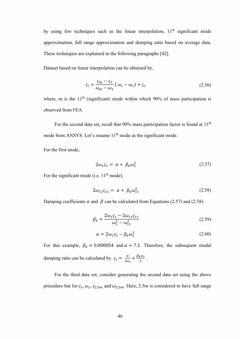
46

by using few techniques such as the linear interpolation, 11th significant mode

approximation, full range approximation and damping ratio based on average data.

These techniques are explained in the following paragraphs [42].

Dataset based on linear interpolation can be obtained by,

𝜍𝑖 =𝜍𝑚 − 𝜍1

𝜔𝑚 − 𝜔1

( 𝜔𝑖 − 𝜔1) + 𝜍1 (2.56)

where, m is the 11th (significant) mode within which 90% of mass participation is

observed from FEA.

For the second data set, recall that 90% mass participation factor is found at 11th

mode from ANSYS. Let’s rename 11th mode as the significant mode.

For the first mode,

2𝜔1𝜍1 = 𝛼 + 𝛽𝑘𝜔12 (2.57)

For the significant mode (i.e. 11th mode),

2𝜔11𝜍11 = 𝛼 + 𝛽𝑘𝜔112 (2.58)

Damping coefficients 𝛼 and 𝛽 can be calculated from Equations (2.57) and (2.58).

𝛽𝑘 =2𝜔1𝜍1 − 2𝜔11𝜍11

𝜔12 − 𝜔11

2 (2.59)

𝛼 = 2𝜔1𝜍1 − 𝛽𝑘𝜔12 (2.60)

For this example, 𝛽𝑘 = 0.000054 and 𝛼 = 7.1. Therefore, the subsequent modal

damping ratio can be calculated by 𝜍𝑖 = 𝛼

2𝜔𝑖+

𝛽𝑘𝜔𝑖

2 .

For the third data set, consider generating the second data set using the above

procedure but for 𝜍1, 𝜔1, 𝜍2.5𝑚 and 𝜔2.5𝑚. Here, 2.5m is considered to have full range

47

approximation. This way we have Rayleigh’s damping coefficients 𝛽𝑘 = 0.0000465

and 𝛼 = 7.9.

The fourth data set is based on the average of the second and the third data sets.

Results of all four data sets are given in Table 2.5.

Estimation of Rayleigh's damping coefficients

Mo

de

nu

mb

er

Natural

Frequency

from

ANSYS

(Hz)

Circular

natural

frequency

from

ANSYS

(rad/sec)

Damping

ratio

based on

linear

interpolation

Damping ratio

based on

11th mode

approximation

Damping

ratio

based on

full range

approximation

Damping

ratio based

on average

data

1 43.436 273.0263 0.0200 0.0200 0.0208 0.0204

2 43.487 273.3469 0.0200 0.0204 0.0208 0.0206

3 47.216 296.7863 0.0205 0.0200 0.0202 0.0201

4 57.635 362.2771 0.0218 0.0196 0.0193 0.0195

5 57.659 362.4280 0.0218 0.0196 0.0193 0.0195

6 112.75 708.7143 0.0287 0.0241 0.0221 0.0231

7 112.76 708.7771 0.0287 0.0241 0.0221 0.0231

8 148.61 934.1200 0.0332 0.0290 0.0259 0.0275

9 193.9 1218.8000 0.0388 0.0358 0.0316 0.0337

10 193.91 1218.8629 0.0388 0.0358 0.0316 0.0337

11 283.15 1779.8000 0.0500 0.0500 0.0436 0.0468

12 294.04 1848.2514 0.0514 0.0518 0.0451 0.0485

13 294.07 1848.4400 0.0514 0.0518 0.0451 0.0485

14 301.26 1893.6343 0.0523 0.0530 0.0461 0.0496

15 301.66 1896.1486 0.0523 0.0531 0.0462 0.0496

16 363.51 2284.9200 0.0601 0.0632 0.0549 0.0590

17 363.72 2286.2400 0.0601 0.0633 0.0549 0.0591

18 387.35 2434.7714 0.0630 0.0672 0.0582 0.0627

19 387.35 2434.7714 0.0630 0.0672 0.0582 0.0627

20 411 2583.4286 0.0660 0.0711 0.0616 0.0664

21 411.04 2583.6800 0.0660 0.0711 0.0616 0.0664

22 476.76 2996.7771 0.0742 0.0821 0.0710 0.0765

23 476.89 2997.5943 0.0742 0.0821 0.0710 0.0766

24 543.47 3416.0971 0.0826 0.0933 0.0806 0.0869

25 543.52 3416.4114 0.0826 0.0933 0.0806 0.0869

26 631.91 3972.0057 0.0936 0.1081 0.0933 0.1007

27 632.02 3972.6971 0.0937 0.1082 0.0934 0.1008

28 649.57 4083.0114 0.0959 0.1111 0.0959 0.1035

Table 2.5: Estimation of Rayleigh's damping coefficients

48

Figure 2.15: Variation of damping ratio with circular natural frequency

It is concluded from above Figure 2.15 that Rayleigh’s damping coefficients

based on 11th mode approximation are closer to that of the linear approximation and

hence they are considered as the input for further dynamic analysis. This data set is also

fed to ANSYS to get the damped natural frequencies.

This procedure is used here as it is simple to get the spreadsheet for different damping

ratio values and corresponding values of Rayleigh’s damping coefficients, which

indeed respect the increasing nature of damping ratio as the mode number increases.

The obtained values of ‘alpha’ and ‘beta-k’ can be fed as the input data for the dynamic

analysis to estimate damped natural frequencies.

0.0000

0.0100

0.0200

0.0300

0.0400

0.0500

0.0600

0 500 1000 1500 2000

Dam

pin

g r

atio

Circular natural frequency in rad/sec

ESTIMATION OF ALPHA AND BETA -K

Damping ratio based on linear interpolation

Damping ratio based on 11th mode approximation

Damping ratio based on full range approximation

Damping ratio based on average data

49

2.7 Formulation for Orthotropic disc

Formulations presented from Section 2.2 to Section 2.5 are limited to the materials

having isotropic property. Nowadays, composite materials have drawn the attention of

researchers in many applications due to their many advantageous properties such as

light weight and higher stiffness to name a few. This section presents in-plane and out-

of-plane vibration analysis of the orthotropic disc.

2.7.1 Modelling strain energy and kinetic energy

In the presented formulation, the principal material coordinate system is used. The

axis 1 is aligned with the fiber direction and the axis 2 is in the plane of the layer and

also perpendicular to the fiber direction. Let axis 3 be in the direction perpendicular to

the layer and also perpendicular to the fiber direction.

Recall the strain energy formulation for isotropic disc described in sub-section 2.1.1,

rewriting it with newly defined coordinate system,

Π𝑜𝑟𝑡ℎ𝑜 = 1

2∫ ∫ ∫ [𝜎1 𝜎2 𝜎3 𝜎12 𝜎23 𝜎13

𝑅𝑜

𝑅𝑖

2𝜋

0

ℎ2

−ℎ2

]

[

휀1

휀2휀3

2휀12

2휀23

2휀13]

𝑟𝑑𝑟 𝑑𝜃 𝑑𝑧 (2.61)

For orthotropic disc, stress-strain relationship is as follows:

[ 𝜎1

𝜎2𝜎3

𝜎23𝜎13

𝜎12]

=

[ 𝐶11

𝐶12

𝐶13

000

𝐶12

𝐶22

𝐶23

000

𝐶13

𝐶23

𝐶33

000

000

𝐶44

00

0000

𝐶55

0

00000

𝐶66]

[

휀1

휀2휀3

2휀23

2휀13

2휀12]

(2.62)

50

Furthermore, the strain-displacement relationship is assumed linear. In cylindrical

coordinate system,

ε1 =∂u1

∂r (2.63)

ε2 =u1

r+

1

r

∂u2

∂θ (2.64)

ε3 =∂u3

∂z (2.65)

ε12 =1

2(1

r

∂u1

∂θ+

∂u2

∂r−

u2

r) (2.66)

ε13 =1

2(∂u1

∂z+

∂u3

∂r) (2.67)

ε23 =1

2(1

r

∂u3

∂θ+

∂u2

∂z) (2.68)

Substituting Equations (2.63) to (2.68) in Equation (2.61), total strain energy of the

orthotropic disc is given by,

Π𝑜𝑟𝑡ℎ𝑜 = 1

2∫ ∫ ∫ 𝐶11 (

∂u1

∂r)2𝑅𝑜

𝑅𝑖

+2𝜋

0

ℎ2

−ℎ2

𝐶22 (u1

r+

1

r

∂u2

∂θ)2

+ 𝐶33 (∂u3

∂z)2

+ 𝐶44 (1

r

∂u3

∂θ+

∂u2

∂z)2

+ 𝐶55 (∂u1

∂z+

∂u3

∂r)2

+ 𝐶66 (1

r

∂u1

∂θ+

∂u2

∂r−

u2

r)

2

+ 2𝐶12 (∂u1

∂r) (

u1

r+

1

r

∂u2

∂θ) + 2𝐶13 (

∂u1

∂r) (

∂u3

∂z)

+ 2𝐶23 (u1

r+

1

r

∂u2

∂θ) (

∂u3

∂z) 𝑟𝑑𝑟 𝑑𝜃 𝑑𝑧

(2.69)

51

Equation (2.69) is derived in non-dimensional form, which is given next:

Π𝑜𝑟𝑡ℎ𝑜 =ℎ

2∫ ∫ ∫ 𝐶11 (

∂u1

∂ζ)22𝜋

0

+1

β

12

−12

𝐶22 (u1

ζ+

1

ζ

∂u2

∂θ)2

+ 𝐶33 (𝑅𝑜

ℎ

∂u3

∂ξ)2

+ 𝐶44 (1

ζ

∂u3

∂θ+

𝑅𝑜

ℎ

∂u2

∂ξ)2

+ 𝐶55 (𝑅𝑜

ℎ

∂u1

∂ξ+

∂u3

∂ζ)2

+ 𝐶66 (1

ζ

∂u1

∂θ+

∂u2

∂ζ−

u2

ζ)

2

+ 2𝐶12 (∂u1

∂ζ) (

u1

ζ+

1

ζ

∂u2

∂θ) + 2𝐶13 (

∂u1

∂ζ) (

𝑅𝑜

ℎ

∂u3

∂ξ)

+ 2𝐶23 (𝑅𝑜

ℎ) (

u1

ζ+

1

ζ

∂u2

∂θ) (

∂u3

∂ξ) ζ 𝑑𝜃 𝑑ζ 𝑑ξ

(2.70)

Similarly, non-dimensional form of total kinetic energy of the orthotropic disc,

𝑇𝑜𝑟𝑡ℎ𝑜 =1

2 𝜌ℎ𝑅𝑜

2 ∫ ∫ ∫ [ (𝜕𝑢1

𝜕𝑡)

2

+ (𝜕𝑢2

𝜕𝑡)2

(𝜕𝑢3

𝜕𝑡)2

] ζ 𝑑𝜃 𝑑ζ 𝑑ξ 2𝜋

0

1

β

−12

−12

(2.71)

Same approach as discussed in Section 2.3.1 and Section 2.3.2 is considered in order to

derive the maximum strain energy and the maximum kinetic energy for the orthotropic

disc.

2.7.2 In-plane and out-of-plane vibration analysis of orthotropic disc

The deformed shape of pure circumferential mode can be best represented by

evaluating Equation (2.50) at n equals to zero. For in-plane vibration analysis of

orthotropic disc, an eigenvalue problem can be formulated in the similar manner as

explained in sub-section 2.3.3.

Similarly, to calculate the frequency of the lowest out-of-plane mode of the orthotropic

disc, Equations (2.43) and (2.45) are evaluated for zero nodal diameter number.

52

Afterwards, displacement polynomials in radial and transverse directions are

substituted in Equation (2.70) and Equation (2.71). Later, Rayleigh-Ritz solutions for

the lowest in-plane mode and the lowest out-of-plane mode are compared with finite

element solutions to validate the results. Material properties of the Graphite-Polymer

composite are given in Table 2.6.

Material

properties

Value Material

properties

Value

𝐸1 155 GPa 𝐺12 4.40 GPa

𝐸2 12.10 GPa 𝐺13 4.40 GPa

𝐸3 12.10 GPa 𝐺23 3.20 GPa

𝑣12 0.248 𝑣23 0.458

𝑣13 0.248 𝜌𝑜𝑟𝑡ℎ𝑜 = 1800

𝑘𝑔

𝑚3

Table 2.6: Material properties of the orthotropic disc [43]

The dimensions of the orthotropic disc are taken the same as that of the isotropic disc,

described in Section 2.5. The simulation is conducted using SHELL 281 and SHELL

181 elements in ANSYS. SHELL 181 is a four-node element with six degrees of

freedom at each node (translations in the X, Y and Z directions and rotations about the

X, Y, and Z axes) as shown in the following Figure 2.16. This type of shell element is

well suited for analysing thin to moderately thick shell structures. Moreover, SHELL

181 is well-suited for linear, and large rotation and/or large strain nonlinear

applications.

53

Figure 2.16: Geometry of SHELL 181 [41]

The following Table 2.7 shows the comparison of the lowest circumferential

mode and the lowest bending mode natural frequencies of C-F disc made of orthotropic

material calculated using Rayleigh-Ritz method and ANSYS.

Lowest in-plane and out-of-plane mode frequencies

Mode

type

Rayleigh-Ritz

solution

(in Hz)

ANSYS solution using

SHELL 281 elements

(in Hz)

ANSYS solution using

SHELL 181 elements

(in Hz)

Circumferential

𝐾 = 𝐿 = 4

75.95 78.86 74.55

Bending

𝐼 = 𝐽 = 𝑃 = 𝑄

= 3

39.71 37.00 37.82

Table 2.7: Comparison of natural frequencies for the orthotropic disc

It is observed from above Table 2.7 that the lowest bending mode natural

frequency of the disc is less than circumferential mode natural frequency. It is because

of the lower stiffness of the orthotropic disc in transverse direction.

54

2.8 Parametric study

Effect of thickness of the disc on the lowest bending mode natural frequency, the

lowest circumferential mode natural frequency and the coupled mode natural

frequencies is depicted in the following Table 2.8. It is concluded that the lowest

bending mode and the coupled mode natural frequencies increase because of the fact

that the stiffness of the disc increases with thickness. The lowest in-plane mode natural

frequency is constant with thickness variation. The dimensions and material properties

are considered as given in Section 2.5.

Mode set Ω of 0.2 m

thickness disc

Ω of 0.3 m

thickness disc

𝑛 = 0

bending

mode

0.2668 0.3919

𝑛 = 0

circumferential

mode

0.61255 0.608

𝑛 = 1

coupled

0.2494 0.3491

𝑛 = 2

coupled

0.3132 0.4485

𝑛 = 3

coupled

0.5992 0.8722

Table 2.8: Variation of non-dimensional frequency parameter with thickness of the

disc

Effect of thickness of the disc made of Graphite-Polymer composite material is shown

in the following Table 2.9.

55

Mode

type

Outer

thickness

(in m)

RR

solution

(Hz)

ANSYS

SHELL

281

element

(Hz)

ANSYS

SHELL

181

element

(Hz)

Circumferential

𝐾 = 𝐿 = 4

0.2 78.84 78.92 74.58

0.3 75.73 78.91 74.73

Bending

𝐽 = 𝑃 = 7, 𝐼 = 𝑄

= 4

0.2 46.67 47.27 48.69

0.3 66.22 65.37 67.42

Table 2.9 : Effect of thickness on in-plane and out-of-plane natural frequencies of

Graphite-Polymer composite disc

Note that higher order polynomial is chosen to represent the bending mode shape of a

composite disc. These are the minimum number of terms required to make the

polynomial mathematically complete. In Equations (2.23), (2.24) and (2.25), chosen

upper limits of summation are shown in Table 2.9. Again, in determining the upper

limits in Equations (2.23) and (2.25) to represent the deformed shape in bending mode

vibrations, the equal number of cross terms in 𝑟 and 𝑧 directions (i.e. 𝐽 = 𝑃 = 7 ) are

chosen to prevent the matrix ill-conditioning.

The variation of non-dimensional frequency parameter √2𝜔2𝑅02 𝜌(1+𝑣)

𝐸 with Poisson’s

ratio is shown in the following Table 2.10.

56

Mode set

Non-dimensional frequency

parameter √2𝜔2𝑅02 𝜌(1+𝑣)

𝐸

𝑣 = 0.33 𝑣 = 0.4

𝑛 = 0

bending

mode

0.2083 0.2243

𝑛 = 0

circumferential

mode

0.5945 0.5945

𝑛 = 1

coupled

0.1745 0.1998

𝑛 = 2

coupled

0.2243 0.2359

𝑛 = 3

coupled

0.4476 0.4527

Table 2.10: Variation of non-dimensional frequency parameter with Poisson’s ratio of

the circular clamped-free disc of uniform thickness

It can be seen from above Table 2.10 that the lowest bending mode natural

frequency increases with the Poisson’s ratio and the lowest circumferential mode

natural frequency decreases with Poisson’s ratio. The numerical data shown in above

Table 2.10 is non-dimensional. The non-dimensional factors associated with Poisson’s

ratio of 0.33 and 0.4 are 246.28 and 240.044 respectively (and they should be multiplied

with respective frequency parameters shown in above Table 2.10 to calculate natural

frequencies).

57

2.9 Conclusion

In this Chapter, the elastic behaviour of the circular disc of uniform thickness is

presented in Section 2.2. In Section 2.3, Rayleigh-Ritz method is presented. The

trigonometric functions in circumferential coordinate are employed in Rayleigh-Ritz

method. In Sections 2.5 and 2.8, free vibration analyses of the circular disc of uniform

thickness made of Structural Steel material and Graphite-Polymer composite material

are presented. A summary of observations is as follows:

For the circular disc made of Graphite-Polymer composite material, the natural

frequency of circumferential mode only depends on the shear modulus of the

material. The circumferential mode natural frequency almost remains constant

with the variation of the disc thickness parameter.

The lowest bending mode natural frequency increases with the thickness in both

isotropic and orthotropic cases.

For the isotropic disc, the lowest bending mode natural frequency increases with

the Poisson’s ratio of the material. The natural frequencies of vibration modes

of higher nodal diameter numbers increase with Poisson’s ratio.

For the moderately thick discs, it is concluded that, the lowest circumferential

mode frequency is higher than the lowest bending mode frequency because of

the fact that the circumferential mode vibration involves shearing, in which the

sole component of deformation is tangential to the disc middle surface and this

behaviour causes the higher stiffness of the disc in circumferential mode

vibration compared to the bending mode vibration in which the sole component

of displacement present is normal to the disc middle surface (although there

exists ‘small’ radial displacement component as explained in Section 2.5).

58

Rayleigh’s damping coefficients calculated based on modal mass participation

yield more realistic damping characteristic of circular clamped-free disc.

59

Chapter 3

Three-dimensional in-plane and out-of-plane vibrations of linearly-

tapered clamped-free disc

3.1 Introduction

This chapter presents the generalized formulation to investigate the lowest in-

plane mode and the lowest out-of-plane mode natural frequencies of the linearly-

tapered disc by proposed solution technique which employs conventional Rayleigh-

Ritz method with finite-element-like modification. Three-dimensional in-plane and

out-of-plane mode vibrations of a circular tapered disc made of isotropic and

orthotropic materials are investigated. In all the parametric studies for the orthotropic

disc, Graphite-Polymer composite material is considered and for the isotropic disc,

Structural Steel material is considered. The material properties of Graphite-Polymer

composite material are given in Table 2.6. The clamped-free boundary condition is

considered in this Chapter. Effect of linear taper on the lowest circumferential mode

and the lowest out-of-plane mode natural frequencies is studied. Rayleigh-Ritz

solutions are compared with the results calculated using ANSYS.

As discussed in Section 1.2, the increasing demand for realistic dynamic analysis

of thick structural components such as a tapered circular disc in automotive or

turbomachinery applications necessitates the requirement for development of robust

three-dimensional models and their solution procedures.

Nowadays, finite element solvers are used increasingly for modelling three-

dimensional problems. Industrial finite element packages make use of 3-D elements

such as tetrahedral, hexahedra etc. One of the major difficulties associated with the use

60

of such 3-D elements is that one needs a large number of elements to solve the static

analysis problem. This fact is quite true for the dynamic analysis also. Again, this makes

the finite element solver to solve a large number of simultaneous equations [44]. In this

Chapter, this problem is tackled with the presented numerical technique.

The GEnx Commercial Aircraft Engine is used for powering Boeing 747-8 and

Boeing 787 Dreamliner. It is the bypass turbofan engine of 21st century consisting of

carbon-fiber composite fan blades. GEnx-1B engine offers advantages in terms of

weight and delivers up to 15% better specific fuel consumption than its predecessors.

This engine has the fan diameter of 111.1 inch and the inner thickness of the blisk is

0.39 m [45]. The later dimension was measured through its CAD drawing. The

following Figure 3.1 shows the front view and isometric view of the same.

Figure 3.1: CAD geometry of turbofan of GEnx

The above Figure 3.1 shows one of the applications of thick circular annular

discs of clamped-free boundary condition. To study the dynamic behaviour of such

blisk, it can be modelled as a thick linearly-tapered disc of clamped-free boundary

condition. To accurately predict the in-plane and out-of-plane vibration responses of

such thick disc, the development of an efficient three-dimensional model is essential.

61

3.2 Modelling

The basic idea in the finite element method is to solve a complicated problem by

replacing it by a simpler one. More specifically, the entire domain of the problem is

represented as an assemblage of subdivisions called finite elements. These elements are

interconnected at the boundaries of the adjacent elements. These specified joints are

called nodes. Generally, we assume the variation of the displacement field (or any other

field variable of interest) inside a finite element using a simple approximation function.

These functions can be represented as the linear combination of constant coefficients

and algebraic displacement terms. By satisfying the boundary condition at a node, such

approximating functions can be defined in terms of the values of field variables (here,

displacement) at the nodes. To derive the elemental equations, the Lagrange functional

can be minimized with respect to each nodal unknown coefficients. Again, the

Lagrange functional can be written as the summation of each element contribution. The

substitution of assumed displacement polynomial which is indeed a function of

unknown nodal value matrix into the minimization of each elemental Lagrange

functional leads to the derivation of elemental mass and elemental stiffness matrices

[44]. Through the proper assemblage of such elemental mass and elemental stiffness

matrices, global stiffness and global mass matrices of the structural system can be

calculated. This way finite element method can be summarized as an element wise

application of Rayleigh-Ritz method.

Recall the explanation given in sub-section 1.3.1 for the Rayleigh-Ritz method.

In this method, an approximate solution to the problem is developed over the entire

domain.

62

In the presented numerical approach, the domain of linearly-tapered disc is

divided into subdomains, similar to finite element method. Further, an approximate

solution to the problem for each element is developed over the entire domain of

linearly-tapered disc, not just over each element as in the case of finite element method.

Hence, this approach leads to less number of terms in the approximate functions needed

to calculate the natural frequencies that are closer to the exact solutions compared to

finite element method.

In the following Figure 3.2, linearly-tapered disc of clamped-free boundary

condition is represented in cylindrical coordinate system. 𝑅𝑖 and 𝑅𝑜 represent the inner

radius and outer radius of the disc respectively. The inner and outer thicknesses of the

disc are indicated by ℎ𝑖 and ℎ𝑜.

As shown in Figure 3.2, the linearly-tapered disc is divided into a number of

divisions, let it be any positive integer number, in order to model the tapered shape of

a non-deformed disc. Midpoint thickness of each division is calculated, and strain

energy and kinetic energy are integrated over the respective division, keeping the

displacement polynomials global over each division. Later, strain energies and kinetic

energies of all divisions are added in order to derive the total strain energy and total

kinetic energy of the linearly-tapered disc.

63

Figure 3.2: Cross-sectional geometry and coordinate system of linearly-tapered disc

3.2.1 Maximum strain energy and maximum kinetic energy

For linearly-tapered disc, total strain energy is derived by adding the strain energy

of each division (which is basically derived by integrating it with reference to midpoint

thickness and respective radius ratio). It is important to note that thickness term and

radius term, according to the respective division, are multiplied inside of the equations

of energies unlike the formulation for the case of the uniform-thickness disc. Again,

recalling that the non-dimensional term 𝑎 =𝑅𝑜

ℎ appears in Equation (2.27), which holds

true for the uniform-thickness disc case, here it must be modified for each division.

Maximum strain energy of linearly-tapered disc is calculated by the following

Equation (3.1):

64

(𝜋𝑚𝑎𝑥)𝐿𝑇

= 𝐸

4(1 + 𝑣)(∫ ∫ ∫ ℎ𝑚𝑖𝑑1 (𝑡𝑒𝑟𝑚𝑠 𝑜𝑓 Π1) ζ𝑑𝜃 𝑑ζ 𝑑ξ

2𝜋

0

1

β1

12

−12

+ ∫ ∫ ∫ ℎ𝑚𝑖𝑑2 (𝑡𝑒𝑟𝑚𝑠 𝑜𝑓 Π2) ζ𝑑𝜃 𝑑ζ 𝑑ξ 2𝜋

0

1

β2

12

−12

+ ∫ ∫ ∫ ℎ𝑚𝑖𝑑3 (𝑡𝑒𝑟𝑚𝑠 𝑜𝑓 Π3) ζ𝑑𝜃 𝑑ζ 𝑑ξ 2𝜋

0

1

β3

12

−12

+ ……… ∫ ∫ ∫ ℎ𝑚𝑖𝑑𝑁 (𝑡𝑒𝑟𝑚𝑠 𝑜𝑓 Π𝑁) ζ𝑑𝜃 𝑑ζ 𝑑ξ 2𝜋

0

1

β𝑁

12

−12

)

(3.1)

where, 𝑡𝑒𝑟𝑚𝑠 𝑜𝑓 Π𝑁 are obtained from Equation (2.26). where, 𝑎𝑁 =𝑅𝑜𝑁

ℎ𝑁 and 𝑁 is the

division number.

𝑡𝑒𝑟𝑚𝑠 𝑜𝑓 Π𝑁 = 2𝑣

1 − 2𝑣((

𝜕𝑈

𝜕ζ) sin 𝑛𝜃 −

𝑛 𝑉 sin 𝑛𝜃

ζ+

𝑈 sin 𝑛𝜃

ζ

+ 𝑎𝑁 (∂W

∂ξsin 𝑛𝜃)

2

) + 2(𝜕𝑈

𝜕ζsin 𝑛𝜃)

2

+ 2(𝑈 sin 𝑛𝜃

ζ−

𝑛 𝑉 sin 𝑛𝜃

ζ)

2

+ 2𝑎𝑁2 (

∂W

∂ξsin 𝑛𝜃)

2

+ (𝑛 𝑈 cos 𝑛𝜃

ζ+

𝜕𝑉

𝜕ζcos 𝑛𝜃 −

𝑉 cos 𝑛𝜃

ζ)2

+ (𝑎𝑁

∂V

∂ξcos 𝑛𝜃 +

𝑛 𝑊 cos 𝑛𝜃

ζ)

2

+ (𝑎𝑁

∂U

∂ξsin 𝑛𝜃 +

𝜕𝑊

𝜕ζsin 𝑛𝜃)

2

(3.2)

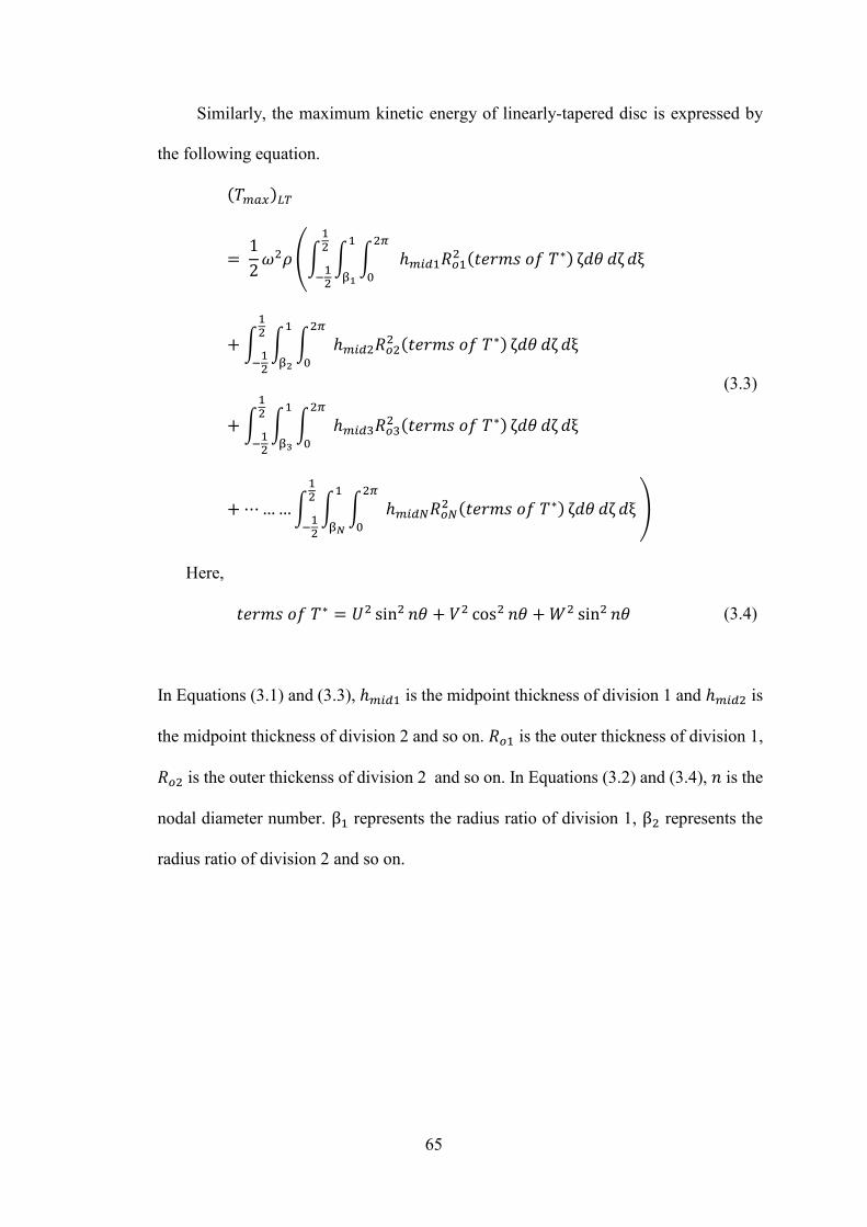
65

Similarly, the maximum kinetic energy of linearly-tapered disc is expressed by

the following equation.

(𝑇𝑚𝑎𝑥)𝐿𝑇

= 1

2𝜔2𝜌 (∫ ∫ ∫ ℎ𝑚𝑖𝑑1𝑅𝑜1

2 (𝑡𝑒𝑟𝑚𝑠 𝑜𝑓 𝑇∗) ζ𝑑𝜃 𝑑ζ 𝑑ξ2𝜋

0

1

β1

12

−12

+ ∫ ∫ ∫ ℎ𝑚𝑖𝑑2𝑅𝑜22 (𝑡𝑒𝑟𝑚𝑠 𝑜𝑓 𝑇∗) ζ𝑑𝜃 𝑑ζ 𝑑ξ

2𝜋

0

1

β2

12

−12

+ ∫ ∫ ∫ ℎ𝑚𝑖𝑑3𝑅𝑜32 (𝑡𝑒𝑟𝑚𝑠 𝑜𝑓 𝑇∗) ζ𝑑𝜃 𝑑ζ 𝑑ξ

2𝜋

0

1

β3

12

−12

+ ⋯……∫ ∫ ∫ ℎ𝑚𝑖𝑑𝑁𝑅𝑜𝑁2 (𝑡𝑒𝑟𝑚𝑠 𝑜𝑓 𝑇∗) ζ𝑑𝜃 𝑑ζ 𝑑ξ

2𝜋

0

1

β𝑁

12

−12

)

Here,

(3.3)

𝑡𝑒𝑟𝑚𝑠 𝑜𝑓 𝑇∗ = 𝑈2 sin2 𝑛𝜃 + 𝑉2 cos2 𝑛𝜃 + 𝑊2 sin2 𝑛𝜃 (3.4)

In Equations (3.1) and (3.3), ℎ𝑚𝑖𝑑1 is the midpoint thickness of division 1 and ℎ𝑚𝑖𝑑2 is

the midpoint thickness of division 2 and so on. 𝑅𝑜1 is the outer thickness of division 1,

𝑅𝑜2 is the outer thickenss of division 2 and so on. In Equations (3.2) and (3.4), 𝑛 is the

nodal diameter number. β1 represents the radius ratio of division 1, β2 represents the

radius ratio of division 2 and so on.

66

3.3 Rayleigh-Ritz solution

Rayleigh’s quotient for the uniform disc is derived in sub-section 2.3.3. For the

linearly-tapered disc, Equation (2.34) is modified as below:

(Ω)2𝐿𝑇 = 2𝜔2

𝜌(1 + 𝑣)

𝐸=

∫ ∫ ∫ ℎ𝑚𝑖𝑑1(𝑡𝑒𝑟𝑚𝑠 𝑜𝑓 Π1) 휁𝑑𝜃 𝑑휁 𝑑𝜉 + ⋯ 2𝜋

0

1

𝛽1

12

−12

+∫ ∫ ∫ ℎ𝑚𝑖𝑑𝑁 (𝑡𝑒𝑟𝑚𝑠 𝑜𝑓 Π𝑁) 휁𝑑𝜃 𝑑휁 𝑑𝜉 2𝜋

0

1

𝛽𝑁

12

−12

∫ ∫ ∫ ℎ𝑚𝑖𝑑1𝑅𝑜12 (𝑡𝑒𝑟𝑚𝑠 𝑜𝑓 𝑇∗) 휁𝑑𝜃 𝑑휁 𝑑𝜉

2𝜋

0

1

𝛽1

12

−12

+ ⋯

+∫ ∫ ∫ ℎ𝑚𝑖𝑑𝑁𝑅𝑜𝑁2 (𝑡𝑒𝑟𝑚𝑠 𝑜𝑓 𝑇∗) 휁𝑑𝜃 𝑑휁 𝑑𝜉

2𝜋

0

1

𝛽𝑁

12

−12

(3.5)

Further, 𝑡𝑒𝑟𝑚𝑠 𝑜𝑓 Π and 𝑡𝑒𝑟𝑚𝑠 𝑜𝑓 𝑇∗ for in-plane mode and out-of-plane mode

vibrations are derived from the generalized formulation for the uniform disc, presented

in Chapter 2. It is important to note that in Equations (3.1) and (3.3), set (B) functions

are employed.

3.3.1 Eigenvalue problem for in-plane vibrations

To calculate the lowest in-plane mode natural frequency of linearly-tapered disc

made of isotropic material, terms of maximum strain energy and maximum kinetic

energy, represented by Equations (3.2) and (3.4) are modified as follows:

t𝑒𝑟𝑚𝑠 𝑜𝑓 Π𝑁 = (𝜕𝑉

𝜕ζ−

𝑉

ζ)2

+ 𝑎𝑁2 (

∂V

∂ξ)2

(3.6)

𝑡𝑒𝑟𝑚𝑠 𝑜𝑓 𝑇∗ = 𝑉2 (3.7)

Let this circumferential amplitude 𝑉 be expressed as the combination of arbitrary

coefficients and non-dimensional radius and non-dimensional thickness terms.

67

𝑉 = ζ(ζ − β)

(1 − β)∑ ∑ 𝐵𝑘𝑙

𝐿

𝑙=0

𝐾

𝑘=0

ζk ξl (3.8)

As shown in Equation (3.8), the same shape function is assumed as in the case of the

uniform disc case. The advantage of presented approach is that it allows to use lower

order polynomial in Equation (3.8). To obtain the best possible approximation of

natural frequencies, arbitrary coefficients are adjusted and non-dimensional frequency

is made stationary. Minimizing Rayleigh's quotient with respect to arbitrary constants,

𝜕(Ω)2

𝐿𝑇

𝜕𝐵𝑘𝑙= 0 (3.9)

The above Equation (3.9) gives the set of (𝐾 + 1)(𝐿 + 1) linear algebraic equations in

terms of arbitrary coefficients. Upon simplifying, one gets:

𝜕𝑁

𝜕𝐵𝑘𝑙− (Ω)2

𝐿𝑇

𝜕𝐷

𝜕𝐵𝑘𝑙= 0 (3.10)

where, 𝑁 and 𝐷 are the numerator and the denominator of Equation (3.5).

Equation (3.10) can be rewritten and represented as an eigenvalue problem:

([𝐾] − (Ω)2𝐿𝑇[𝑀]){𝐵𝑘𝑙} = {0} (3.11)

To have a non-trivial solution, let the determinant of the augmented matrix be

zero in Equation (3.11). MATLAB code is developed to get the non-dimensional

frequency parameter (Ω)𝐿𝑇 = √2𝜔2 𝜌(1+𝑣)

𝐸 and subsequently the natural frequency of

in-plane mode vibration of the disc made of isotropic material is obtained.

3.3.2 Eigenvalue problem for out-of-plane vibrations

To investigate out-of-plane vibrations of the linearly-tapered disc, Equations (3.2)

and (3.4) are recalculated again using set (A) functions expressed as Equations (2.43),

(2.44) and (2.45), which hold true for bending mode and coupled modes. Further, these

equations are recalculated for 𝑛 = 0 to calculate the lowest bending natural frequency.

68

For pure transverse mode, the amplitudes in 𝑟 and 𝑧 directions are expressed by

Equations (2.23) and (2.25) respectively.

3.4 Parametric study on isotropic disc

It is assumed that linearly-tapered disc is made of Structural Steel material. The

numerical values of Young’s modulus and Poisson’s ratio for this material are 200 GPa

and 0.3 respectively. The outer radius and inner radius of the linearly-tapered disc are

0.5 m and 0.1 m respectively. The inner thickness of linearly-tapered disc is 0.4 m and

kept constant throughout the analysis.

Rayleigh-Ritz solutions are compared with the results calculated using ANSYS.

In simulation using ANSYS, SOLID 186 elements are used along with quadratic

hexahedral mesh type in order to get accurate results compared to the tetrahedral

elements without mid-side nodes. SOLID 186 is a higher-order three-dimensional 20-

node element. This element has three translation degrees of freedom per node and it

exhibits quadratic displacement behaviour.

3.4.1 In-plane vibrations of linearly-tapered isotropic disc

To study the effect of linear taper on the lowest in-plane mode frequency, consider

that the outer thickness of the linearly-tapered disc is varied up to 0.2 m. As shown in

the following Figure 3.3, for all of the three radius ratios namely 0.2, 0.25 and 0.3, it is

observed that the lowest in-plane mode frequency increases with the decrease of outer

thickness.

69

Figure 3.3: Variation of the lowest in-plane mode frequency with outer thickness

and radius ratio

As discussed in Section 1.1, in some of the engineering applications of circular

tapered discs, it is advisable to study the effect of linear taper on the lowest in-plane

mode frequency. Consider the variation of taper angle from infinitesimal taper up to 1

degree of taper. The following Figure 3.4 shows the variation of the lowest in-plane

mode frequency with taper angle for radius ratio of 0.3.

1

1.2

1.4

1.6

1.8

2

2.2

2.4

0.39 0.35 0.3 0.25 0.2

Non-d

imes

ional

fre

quen

cy p

aram

eter

Outer thickness of linearly-tapered disc (in m)

Effect of linear taper on lowest in-plane mode frequency

RR solution for radius

ratio 0.2

Non-dimensional

frequency parameter for

radius ratio 0.2

calculated using

ANSYSRR solution for radius

ratio 0.25

Non-dimensional

frequency parameter for

radius ratio 0.25

calculated using

ANSYSRR solution for radius

ratio 0.3

Non-dimensional

frequency parameter for

radius ratio 0.3

calculated using

ANSYS

70

Figure 3.4: Variation of the lowest in-plane mode frequency with taper angle of

linearly-tapered isotropic disc for beta value of 0.3

3.4.2 Out-of-plane vibrations of linearly-tapered isotropic disc

The following Figure 3.5 shows the effect of linear taper on the lowest bending

mode non-dimensional frequency parameter. This study concludes that the non-

dimensional frequency parameter of lowest bending mode increases linearly with taper-

angle.

Figure 3.5: Variation of the lowest transverse mode frequency with taper angle of

linearly-tapered isotropic disc for beta value of 0.25

1.861.88

1.91.921.94

0.2 0.4 0.6 0.8 1N

on

-dim

ensi

on

al

freq

uen

cy p

aram

eter

Taper angle (in degrees)

RR solution for lowest in-plane mode

Non-dimensional frequency parameter for lowest in-plane mode from ANSYS

2.3

2.35

2.4

2.45

2.5

2.55

0.2 0.4 0.6 0.8 1

No

n-d

imen

sio

nal

fre

qu

ency

p

aram

eter

Taper angle (in degrees)

RR solution

ANSYS

71

Comparison of lowest transverse mode non-dimensional frequency obtained using

Rayleigh-Ritz solution and Finite Element solution is made for radius ratio values of

0.2 and 0.25 in the following Figure 3.6.

Figure 3.6: Variation of the lowest transverse mode frequency with linear taper and

radius ratio

It is noted from the present three-dimensional analysis that the non-dimensional

frequency parameter for the isotropic disc, calculated using ANSYS are higher than

that obtained using Rayleigh-Ritz method. Moreover, higher mode vibration analysis

can be conducted with acceptable accuracy using presented formulation.

3.5 Vibration analysis of linearly-tapered orthotropic disc

Formulation derived in sub-section 3.2.1 is limited to a linearly-tapered disc of

clamped-free boundary condition made of isotropic material. In the present section, the

generalized formulation for the orthotropic disc of linearly-varying thickness is

0.39 0.35 0.3 0.25 0.2

RR solution for radius ratio0.2

1.902010098 1.942 2 2.0643 2.1423

Non-dimensional frequencyparameter for radius ratio0.2 calculated using ANSYS

2.230830547 2.298738475 2.383346314 2.482706897 2.602519127

RR solution for radius ratio0.25

2.378 2.410225006 2.456813392 2.511738223 2.578088557

Non-dimensional frequencyparameter for radius ratio

0.25 calculated using ANSYS2.489421737 2.573349796 2.66900336 2.784411788 2.920786699

1.5

1.7

1.9

2.1

2.3

2.5

2.7

2.9

3.1

No

n-d

imen

sio

nal

fr

equ

ency

par

amet

er

Outer thickness of linearly-tapered disc

72

developed to study the effect of linear taper on the lowest in-plane mode and the lowest

out-of-plane mode natural frequencies based on the approach discussed in Section 3.2.

For the orthotropic disc, midpoint thickness of each division is calculated.

Maximum strain energy and maximum kinetic energy for each division are integrated

uniformly over respective division considering the formulation for uniform thickness

orthotropic disc case as described in Section 2.7. Material properties of Graphite-

Polymer composite as given in Table 2.6, are considered for the present analysis.

3.5.1 In-plane vibrations of linearly-tapered orthotropic disc

To investigate three-dimensional in-plane vibration response, maximum strain

energy and maximum kinetic energy of linearly-tapered clamped-free orthotropic disc

are calculated as follow:

(𝜋𝑚𝑎𝑥)𝐿𝑇 = 0.5𝐶66 (∫ ∫ ∫ 2𝜋

0

1

β1

12

−12

ℎ𝑚𝑖𝑑1 [𝐶44

𝐶66𝑎𝑁

2 (∂V

∂ξ)2

+ (𝜕𝑉

𝜕ζ−

𝑉

ζ)

2

] ζ𝑑𝜃 𝑑ζ 𝑑ξ + ⋯

+ ∫ ∫ ∫ 2𝜋

0

1

β𝑁

12

−12

ℎ𝑚𝑖𝑑𝑁 [𝐶44

𝐶66𝑎𝑁

2 (∂V

∂ξ)2

+ (𝜕𝑉

𝜕ζ−

𝑉

ζ)

2

] ζ𝑑𝜃 𝑑ζ 𝑑ξ)

(3.12)

(𝑇𝑚𝑎𝑥)𝐿𝑇 = 1

2𝜔2𝜌𝑜

(

∫ ∫ ∫ ℎ𝑚𝑖𝑑1𝑅𝑜12 𝑉2 휁𝑑𝜃𝑑휁 𝑑𝜉

2𝜋

0

1

𝛽1

12

−12

+ ⋯

+∫ ∫ ∫ ℎ𝑚𝑖𝑑𝑁𝑅𝑜𝑁2 𝑉2 휁𝑑𝜃 𝑑휁 𝑑𝜉

2𝜋

0

1

𝛽𝑁

12

−12 )

(3.13)

where, 𝜌𝑜 is the density of orthotropic material.

73

From Equations (3.12) and (3.13), the frequency parameter can be obtained as follows:

(Ω)𝐿𝑇𝑜 = √𝜌𝑜 𝜔2

𝐶66 (3.14)

Again, it is minimized with respect to the arbitrary coefficients to calculate the

approximate natural frequency of the lowest in-plane mode. Polynomial described by

Equation (3.8) is used here for the three-dimensional in-plane mode vibration analysis

of orthotropic disc. MATLAB code is written to solve the eigenvalue problem of a

linearly-tapered orthotropic disc having clamped-free boundary condition.

3.5.2 Transverse vibrations of linearly-tapered orthotropic disc

To study three-dimensional out-of-plane vibrations, maximum strain energy and

maximum kinetic energy of linearly-tapered clamped-free orthotropic disc are

calculated as follow:

(𝜋𝑚𝑎𝑥)𝐿𝑇 =𝐶55

2(∫ ∫ ∫

2𝜋

0

1

β1

12

−12

ℎ𝑚𝑖𝑑1[𝑡𝑒𝑟𝑚𝑠 𝑜𝑓 Π1]𝑜𝑟𝑡ℎ𝑜 ζ𝑑𝜃 𝑑ζ 𝑑ξ

+ ⋯

+ ∫ ∫ ∫ 2𝜋

0

1

β𝑁

12

−12

ℎ𝑚𝑖𝑑𝑁[𝑡𝑒𝑟𝑚𝑠 𝑜𝑓 Π𝑁]𝑜𝑟𝑡ℎ𝑜 ζ𝑑𝜃 𝑑ζ 𝑑ξ)

(3.15)

(𝑇𝑚𝑎𝑥)𝐿𝑇 = 1

2𝜔2𝜌𝑜

(

∫ ∫ ∫ ℎ𝑚𝑖𝑑1𝑅𝑜12 (𝑈2 + 𝑊2) 휁𝑑𝜃 𝑑휁 𝑑𝜉

2𝜋

0

1

𝛽1

12

−12

+ ⋯

+∫ ∫ ∫ ℎ𝑚𝑖𝑑𝑁𝑅𝑜𝑁2 (𝑈2 + 𝑊2) 휁𝑑𝜃 𝑑휁 𝑑𝜉

2𝜋

0

1

𝛽𝑁

12

−12 )

(3.16)

74

where,

[𝑡𝑒𝑟𝑚𝑠 𝑜𝑓 Π𝑁]𝑜𝑟𝑡ℎ𝑜

=𝐶11

𝐶55(𝜕𝑈

𝜕ζ)2

+𝐶22

𝐶55

𝑈2

ζ2+

𝐶33

𝐶55𝑎𝑁

2 (𝜕𝑊

𝜕ξ)2

+ (𝑎𝑁

𝜕𝑈

𝜕ξ+

𝜕𝑊

𝜕ζ)2

+ 2𝐶12

𝐶55

𝑈

ζ

𝜕𝑈

𝜕ζ+ 2𝑎𝑁

𝐶13

𝐶55

𝜕𝑈

𝜕ζ

𝜕𝑊

𝜕ξ

+ 2𝑎𝑁

𝐶23

𝐶55

𝑈

ζ

𝜕𝑊

𝜕ξ

(3.17)

Equations (3.15) and (3.16) are equated and non-dimensional frequency parameter for

the lowest transverse mode can be calculated as follows:

(Ω)𝐿𝑇𝑜 = √𝜌𝑜 𝜔2

𝐶55 (3.18)

This frequency parameter is minimized with respect to the arbitrary coefficients

of Equations (2.23) and (2.25). MATLAB code is developed to solve the eigenvalue

problem and as a result, the lowest frequency parameter for the lowest transverse mode

is reported.

3.6 Parametric study on orthotropic discs

The three-dimensional response of the linearly-tapered disc made of the Graphite-

Polymer composite material is studied using the presented approach. The same

dimensions of the orthotropic disc are considered as that of the isotropic disc. The inner

thickness and outer radius of the disc are kept constant throughout the analysis.

Rayleigh-Ritz solutions are compared with results calculated using ANSYS. Effect of

taper angle and radius ratio on the lowest in-plane mode and the lowest out-of-plane

mode natural frequencies is studied. Moreover, three-dimensional higher mode

75

vibration analysis for the linearly-tapered disc of orthotropic material also can be

conducted with good accuracy with the presented formulation.

The following Figure 3.7 shows the bending mode and circumferential mode

vibration of linearly tapered circular disc of beta value of 0.2 (and taper angle of 14.04)

and made of Graphite-Polymer composite material. In ANSYS, free vibration analysis

was conducted using SOLID 186 elements. For the mentioned disc, the fundamental

mode of vibration is the circumferential mode.

Figure 3.7: The lowest bending and the lowest circumferential mode vibrations of

linearly-tapered disc made of Graphite-Polymer composite material having beta value

of 0.2

The following Figure 3.8 shows a variation of frequency parameter with outer thickness

of the disc and radius ratio. Lower order polynomial in 𝑟 and 𝑧 is used along with

considering 5, 3 and 2 numbers of divisions for the orthotropic disc of radius ratio 0.2,

0.25 and 0.3 respectively to calculate the lowest in-plane mode frequency.

76

Figure 3.8: Variation of the lowest in-plane mode natural frequency of linearly-

tapered orthotropic disc with respect to linear-taper and radius ratio

From above Figure 3.8, it is observed that for the linearly-tapered orthotropic disc,

the increase in frequency parameter is non-linear with linear increment of radius ratio.

For example, for linearly-tapered disc of outer radius of 0.3, frequency parameters

calculated using Rayleigh-Ritz method with finite-element-like modification are

1.1860, 1.538 and 1.9414 for beta values of 0.2, 0.25 and 0.3 respectively.

The variation of the frequency parameters of the lowest in-plane mode with taper

angle for different radius ratio values are depicted in the following Figure 3.9. It is

observed that for the orthotropic disc, the frequency parameters increase with taper

angle and radius ratio.

1

1.2

1.4

1.6

1.8

2

2.2

2.4

0.39 0.35 0.3 0.25 0.2

Freq

uen

cy p

aram

eter

Outer thickness of linearly-tapered orthotropic disc (in m)

Effect of linear taper on the lowest in-plane mode

frequency of orthotropic discRR solution for beta

value of 0.2

Non-dimensional

frequency parameter

for beta value of 0.2

calculated using

ANSYS

RR solution for beta

value of 0.25

RR solution for beta

value of 0.3

77

Figure 3.9: Behaviour of orthotropic disc in in-plane vibration mode with respect to

taper angle and radius ratio

The natural frequency for the lowest transverse mode of the orthotropic disc is

calculated using Rayleigh-Ritz method for the beta value of 0.2 and the variation of

natural frequency with outer thickness of the disc is noted in the following Table 3.1.

For a disc of radius ratio 0.2, lower order polynomial is considered along with six

number of divisions.

1

1.2

1.4

1.6

1.8

2

0.2 0.4 0.6 0.8 1

Freq

uen

cy p

aram

eter

Taper angle of orthotropic disc (in degrees)

Behaviour of linearly-tapered orthotropic disc in

in-plane vibration mode

RR solution for beta value of 0.2

Non-dimensional frequencyparameter for beta value of 0.2calculated using ANSYS

RR solution for beta value of 0.25

RR solution for beta value of 0.3

78

Outer

thickness

(ℎ𝑜 in m)

Taper angle

(in degrees)

RR solution

(𝑓3 in Hz)

Finite element

solution using

ANSYS

%

Difference

0.39 0.72 583.4589 573.84 -1.68

0.35 3.58 595.4906 589.29 -1.05

0.3 7.12 612.5969 611.18 -0.23

0.25 10.62 632.5566 636.65 0.64

0.2 14.04 656.1879 666.94 1.61

Table 3.1: Variation of natural frequency of the lowest transverse mode with outer

thickness of linearly-tapered orthotropic disc for beta value of 0.2

In Equations (2.23) and (2.25), the upper limit of summation is set to 1 (i.e. four

terms in the polynomial are considered) to analyse the three-dimensional out-of-plane

vibration response of orthotropic disc having a beta value of 0.25. Here, four number

of divisions are considered to determine approximate frequencies.

In above Table 3.1, percentage difference is calculated using the following

formula:

% Difference =3D FEA solution − 3D RR solution

3D FEA solution (3.19)

In Table 3.1, taper angle is calculated using the following formula:

𝑡𝑎𝑝𝑒𝑟 𝑎𝑛𝑔𝑙𝑒 = 90 − tan−12(𝑅𝑜 − 𝑅𝑖)

ℎ𝑖 − ℎ𝑜 (3.20)

where, ℎ𝑖 and ℎ𝑜 are the inner and outer thicknesses of the tapered disc and 𝑅𝑖 and 𝑅𝑜

are the inner and outer radius values of the tapered disc. The following Table 3.2 shows

the variation of natural frequency with the outer thickness of the disc.

79

Outer

thickness

(ℎ𝑜 in m)

Taper angle

(in degrees)

RR solution

(𝑓3 in Hz)

Finite element

solution using

ANSYS

%

Difference

0.39 0.76 666.1490 640.57 -3.99

0.35 3.81 677.2914 658.28 -2.89

0.3 7.59 693.1765 683.25 -1.45

0.25 11.31 711.7809 712.13 0.05

0.2 14.93 733.9158 746.27 1.66

Table 3.2: Variation of natural frequency of lowest transverse mode with outer

thickness of linearly-tapered orthotropic disc for beta value of 0.25

Variation of natural frequency of the lowest transverse mode with outer thickness of

disc is shown in Table 3.3, which is given below:

Outer

thickness

(ℎ𝑜 in m)

Taper angle

(in degrees)

RR solution

(𝑓3 in Hz)

Finite element

solution using

ANSYS

%

Difference

0.39 0.82 739.5735 715.87 -3.31

0.35 4.09 749.3756 736.27 -1.78

0.3 8.13 763.3466 764.88 0.20

0.25 12.09 779.7100 797.73 2.26

0.2 15.95 800.0 836.31(𝑓4) 4.34

Table 3.3: Variation of natural frequency of the lowest transverse mode with outer

thickness of linearly-tapered orthotropic disc for beta value of 0.3

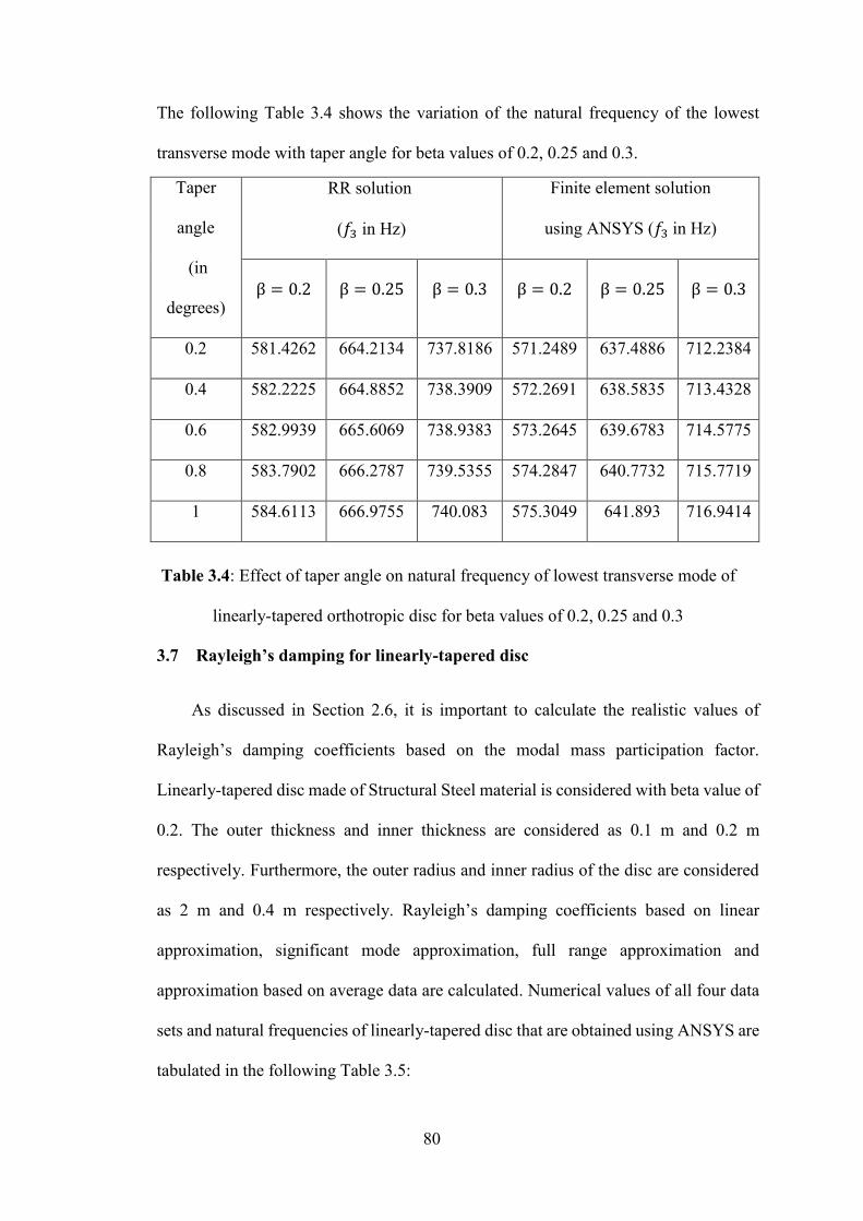
80

The following Table 3.4 shows the variation of the natural frequency of the lowest

transverse mode with taper angle for beta values of 0.2, 0.25 and 0.3.

3.7 Rayleigh’s damping for linearly-tapered disc

As discussed in Section 2.6, it is important to calculate the realistic values of

Rayleigh’s damping coefficients based on the modal mass participation factor.

Linearly-tapered disc made of Structural Steel material is considered with beta value of

0.2. The outer thickness and inner thickness are considered as 0.1 m and 0.2 m

respectively. Furthermore, the outer radius and inner radius of the disc are considered

as 2 m and 0.4 m respectively. Rayleigh’s damping coefficients based on linear

approximation, significant mode approximation, full range approximation and

approximation based on average data are calculated. Numerical values of all four data

sets and natural frequencies of linearly-tapered disc that are obtained using ANSYS are

tabulated in the following Table 3.5:

Taper

angle

(in

degrees)

RR solution

(𝑓3 in Hz)

Finite element solution

using ANSYS (𝑓3 in Hz)

β = 0.2 β = 0.25 β = 0.3 β = 0.2 β = 0.25 β = 0.3

0.2 581.4262 664.2134 737.8186 571.2489 637.4886 712.2384

0.4 582.2225 664.8852 738.3909 572.2691 638.5835 713.4328

0.6 582.9939 665.6069 738.9383 573.2645 639.6783 714.5775

0.8 583.7902 666.2787 739.5355 574.2847 640.7732 715.7719

1 584.6113 666.9755 740.083 575.3049 641.893 716.9414

Table 3.4: Effect of taper angle on natural frequency of lowest transverse mode of

linearly-tapered orthotropic disc for beta values of 0.2, 0.25 and 0.3

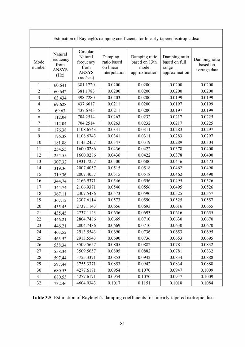
81

Estimation of Rayleigh's damping coefficients for linearly-tapered isotropic disc

Mode

number

Natural

frequency

from

ANSYS

(Hz)

Circular

Natural

frequency

from

ANSYS

(rad/sec)

Damping

ratio based

on linear

interpolation

Damping ratio

based on 13th

mode

approximation

Damping ratio

based on full

range

approximation

Damping ratio

based on

average data

1 60.641 381.1720 0.0200 0.0200 0.0200 0.0200

2 60.642 381.1783 0.0200 0.0200 0.0200 0.0200

3 63.434 398.7280 0.0203 0.0200 0.0199 0.0199

4 69.628 437.6617 0.0211 0.0200 0.0197 0.0199

5 69.63 437.6743 0.0211 0.0200 0.0197 0.0199

6 112.04 704.2514 0.0263 0.0232 0.0217 0.0225

7 112.04 704.2514 0.0263 0.0232 0.0217 0.0225

8 176.38 1108.6743 0.0341 0.0311 0.0283 0.0297

9 176.38 1108.6743 0.0341 0.0311 0.0283 0.0297

10 181.88 1143.2457 0.0347 0.0319 0.0289 0.0304

11 254.55 1600.0286 0.0436 0.0422 0.0378 0.0400

12 254.55 1600.0286 0.0436 0.0422 0.0378 0.0400

13 307.32 1931.7257 0.0500 0.0500 0.0446 0.0473

14 319.36 2007.4057 0.0515 0.0518 0.0462 0.0490

15 319.36 2007.4057 0.0515 0.0518 0.0462 0.0490

16 344.74 2166.9371 0.0546 0.0556 0.0495 0.0526

17 344.74 2166.9371 0.0546 0.0556 0.0495 0.0526

18 367.11 2307.5486 0.0573 0.0590 0.0525 0.0557

19 367.12 2307.6114 0.0573 0.0590 0.0525 0.0557

20 435.45 2737.1143 0.0656 0.0693 0.0616 0.0655

21 435.45 2737.1143 0.0656 0.0693 0.0616 0.0655

22 446.21 2804.7486 0.0669 0.0710 0.0630 0.0670

23 446.21 2804.7486 0.0669 0.0710 0.0630 0.0670

24 463.52 2913.5543 0.0690 0.0736 0.0653 0.0695

25 463.52 2913.5543 0.0690 0.0736 0.0653 0.0695

26 558.34 3509.5657 0.0805 0.0882 0.0781 0.0832

27 558.34 3509.5657 0.0805 0.0882 0.0781 0.0832

28 597.44 3755.3371 0.0853 0.0942 0.0834 0.0888

29 597.44 3755.3371 0.0853 0.0942 0.0834 0.0888

30 680.53 4277.6171 0.0954 0.1070 0.0947 0.1009

31 680.53 4277.6171 0.0954 0.1070 0.0947 0.1009

32 732.46 4604.0343 0.1017 0.1151 0.1018 0.1084

Table 3.5: Estimation of Rayleigh’s damping coefficients for linearly-tapered isotropic disc

82

The Rayleigh’s damping coefficients based on full range approximation are

calculated as explained in Section 2.6. The value of Alpha-lt and Beta-klt based on full

range approximation are 8.88 and 0.0000438 respectively, which match the best with

the datum value calculated based on linear interpolation.

The following Figure 3.10 shows the variation of damping ratio with circular

natural frequency of the linearly-tapered circular disc of clamped-free boundary

condition.

Figure 3.10: Variation of damping ratio with circular natural frequency of linearly-

tapered isotropic disc

0.0000

0.0200

0.0400

0.0600

0.0800

0.1000

0.1200

0.1400

0 500 1000 1500 2000 2500 3000 3500 4000 4500 5000

Dam

pin

g ra

tio

Circular natural frequency in rad/sec

Estimation of alpha-lt and beta-klt

Damping ratio based on linear interpolation

Damping ratio based on 13th mode approximation

Damping ratio based on full range approximation

Damping ratio based on average data

83

It is observed from above Figure 3.10 that the damping ratio variation is not significant

for the frequency range from 381.1720 rad/sec to 704.2514 rad/sec.

3.8 Conclusion

In this Chapter, free vibration analysis of linearly-tapered circular disc of

clamped-free boundary condition has been conducted. Frequency parameters for the

discs made of orthotropic and isotropic material have been reported using Rayleigh-

Ritz method with finite-element-like modification. For the circular tapered disc made

of Graphite-Polymer composite material, the frequency parameters obtained from the

presented approach are in good agreement (less than 5% difference is noted) when

compared with 3-D finite element solutions using ANSYS. A summary of observations

is as follows:

An efficient and accurate approximate solution for 3-D vibration response of

clamped-free isotropic and orthotropic discs has been developed using Rayleigh-

Ritz method. Linear strains are considered for the analysis. The presented

solution will be useful to check the accuracy of the approximate solutions derived

using 2-D approach.

The presented approach allows one to use the lower order polynomials to

calculate the lowest in-plane and the lowest out-of-plane natural frequencies for

the linearly-tapered clamped-free circular disc. Moreover, the free-vibration

analysis can be conducted using presented formulation for the clamped-clamped

and free-clamped boundary conditions considering appropriate constraint

functions in displacements polynomials. The clamped-clamped disc has found

application as locking device, which locks the connecting machine components

84

to each other by hydraulic pressure. The free-clamped disc has found application

as clamping device (or fixture), which basically holds the machining tool.

The frequency parameters of the in-plane vibration mode solely depends on shear

modulus of the composite material.

The frequency parameter for the lowest circumferential mode and the lowest

bending mode increase with radius ratio.

The variation of lowest bending mode natural frequency with taper angle is

higher when the radius ratio increases.

For the considerably-thick linearly-tapered disc (with 𝑅𝑜

ℎ𝑖 value of 1.25), it is

observed that the fundamental mode of vibration is the circumferential mode.

For the thick disc case, the bending stiffness of the structure is higher compared

to in-plane stiffness.

85

Chapter 4

Three-dimensional in-plane and out-of-plane vibrations of non-

linearly tapered clamped-free disc

4.1 Introduction

The circular discs of non-linear thickness variation have found applications in

turbomachinery. Very specific type of non-linear taper is considered in this Chapter

which is defined by the hyperbolic taper. Here, hyperbolic thickness variation along

radial direction is represented by the equation 𝑡 =𝑡1

𝑟𝑠 , where ‘s’ is the taper parameter

of the disc. Circular disc with such a thickness variation is often known as Stodola’s

disc and has wide range of applications as discussed in Chapter 1. It has higher

thickness at inner radius and lower thickness at outer radius. In this Chapter, three-

dimensional free vibration of Stodola’s disc is studied based on the numerical technique

developed in the Chapter 3. Parametric study on in-plane and out-of-plane mode natural

frequencies of isotropic and orthotropic discs based on the taper parameter of Stodola’s

disc is conducted. For the parametric studies on orthotropic Stodola’s disc and isotropic

Stodola’s disc, Graphite-Polymer composite material and Structural Steel material are

considered respectively. The material properties of Graphite-Polymer composite

material are given in Table 2.6. Throughout this Chapter, clamped-free boundary

condition is considered.

4.2 Modelling

As shown in the following Figure 4.1, Stodola’s disc is divided into a number of

divisions to model the non-linear tapered shape of non-deformed Stodola’s disc. Similar

approach as mentioned in Chapter 3 is developed to study free vibration behaviour of

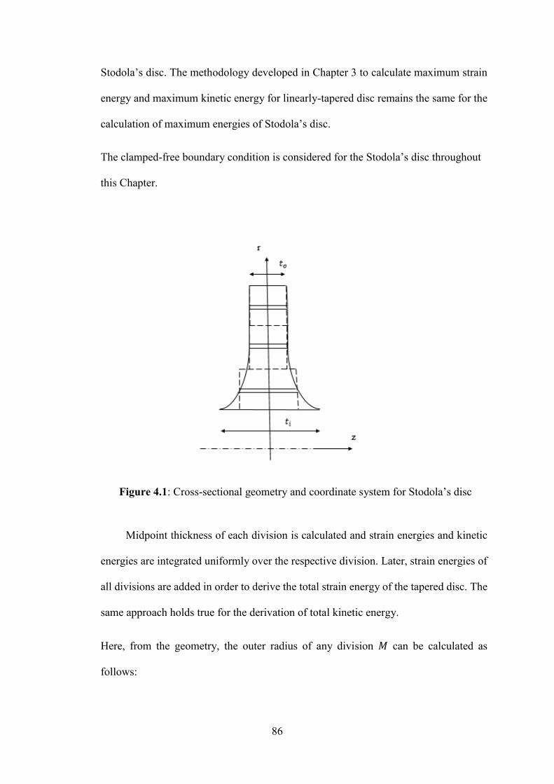
86

Stodola’s disc. The methodology developed in Chapter 3 to calculate maximum strain

energy and maximum kinetic energy for linearly-tapered disc remains the same for the

calculation of maximum energies of Stodola’s disc.

The clamped-free boundary condition is considered for the Stodola’s disc throughout

this Chapter.

Figure 4.1: Cross-sectional geometry and coordinate system for Stodola’s disc

Midpoint thickness of each division is calculated and strain energies and kinetic

energies are integrated uniformly over the respective division. Later, strain energies of

all divisions are added in order to derive the total strain energy of the tapered disc. The

same approach holds true for the derivation of total kinetic energy.

Here, from the geometry, the outer radius of any division 𝑀 can be calculated as

follows:

87

𝑅𝑜𝑁 = 𝑅𝑖 + 𝑀 𝑙𝑟 (4.1)

where 𝑀 is the number of divisions and 𝑙𝑟 is the radial length of each (equal) division.

𝑅𝑖 is the inner radius of the Stodola’s disc.

Similarly, radius ratio for each division can be calculated using following formula,

𝛽𝑁 = 𝑅𝑖 + (𝑀 − 1) 𝑙𝑟

𝑅𝑖 + 𝑀 𝑙𝑟 (4.2)

Midpoint thickness of 𝑀𝑡ℎ division can be calculated as follows:

ℎ𝑚𝑖𝑑𝑀 =ℎ𝑖𝑀 + ℎ𝑜𝑀

2 (4.3)

Here,

ℎ𝑜𝑀 = ℎ𝑖𝑅𝑖

𝑠

(𝑅𝑖 + (𝑀 − 1)𝑙𝑟)𝑠 (4.4)

Equations (3.1) and (3.3) are modified in accordance with Equation (4.2) and (4.3)

to calculate maximum strain energy and maximum kinetic energy of Stodola’s disc

made of isotropic material and subsequently to study the in-plane and out-of-plane

mode vibrations characteristics.

To study the three-dimensional vibrations of Stodola’s disc made of a Graphite-

Polymer composite material, Equations (3.12) and (3.13) should be modified by

considering Equations (4.2) and (4.3).

88

4.3 Parametric study on isotropic Stodola’s discs

It is assumed that the non-linearly tapered disc is made of Structural Steel

material. Young’s modulus and Poisson’s ratio for this material are 200 GPa and 0.3

respectively. Non-dimensional frequency parameters are calculated using Rayleigh-

Ritz method with finite-element-like modification and compared with the three-

dimensional ANSYS solutions. Three-dimensional in-plane vibration frequencies are

noted in following Table 4.1 for different taper parameters of Stodola’s disc and for

radius ratio of 0.2. The inner thickness of Stodola’s disc is 0.4 m and kept constant

throughout the analysis.

Taper

Parameter

‘s’

Outer

thickness

(in m)

RR solution

(𝑓1) in Hz

ANSYS

Solution (in Hz)

% Difference

from ANSYS

(hex mesh)

solution

Hex

mesh

Tet

mesh

0.861353 0.1 859.7902 853.45 854.62 -0.74

0.609423 0.15 736.8296 773.25 774.96 4.71

0.430677 0.2 702.7748 719.43 721.48 2.31

0.29203 0.25 677.2498 678.81 680.44 0.23

0.178747 0.3 657.0184 645.88 647.31 -1.72

Table 4.1: Variation of natural frequency of the lowest in-plane mode with taper

parameter of Stodola’s disc for beta value of 0.2

For non-rotating Stodola’s disc, the circumferential in-plane mode is the fundamental

mode of vibration. For the disc of beta value of 0.2, three numbers of divisions are

considered for the disc of taper parameter value 0.861353 and for rest of the

89

configurations of non-linear tapers, four numbers of divisions are considered. The lower

order shape function has been considered with 𝐾 = 𝐿 = 1 in Equation (2.24).

In the lowest bending mode, 𝑧-direction and 𝑟-direction deformations are coupled. The

natural frequencies of the lowest bending mode are presented in the following Table

4.2. For the bending mode vibration analysis of Stodola’s disc, two numbers of

divisions are considered for all the taper parameter values for beta value of 0.2. In

Equations (2.23) and (2.25), the values of 𝐼, 𝐽 and 𝑃, 𝑄 are considered as 2.

Taper

Parameter

‘s’

Outer

thickness

(in m)

RR solution

(𝑓3) in Hz

ANSYS

Solution (in Hz)

% Difference

from ANSYS

(hex mesh)

solution

Hex

Mesh

Tet

mesh

0.861353 0.1 1143.6069 1179.9 1180.5 3.07

0.609423 0.15 1204.9378 1223.5 1224.1 1.52

0.430677 0.2 1180.9205 1221.6 1222.0 3.33

0.29203 0.25 1165.945 1200.5 1200.8 2.88

0.178747 0.3 1154.9725 1171.3 1172.3 1.39

Table 4.2: Variation of natural frequency of the lowest bending mode with taper

parameter of Stodola’s disc for beta value of 0.2

90

4.4 Parametric study on orthotropic Stodola’s discs

It is assumed that Stodola’s disc is made of Graphite-Polymer composite material.

Material properties as given in Table 2.6 are considered. Variation of the lowest in-

plane mode natural frequency with taper parameter and radius ratio is presented in the

following Table 4.3.

Outer

thick-

ness

(in m)

Taper

Parameter

‘s’ for

𝛽 = 0.2

RR

solution

(𝑓1) in Hz

β = 0.2

Taper

Parameter

‘s’ for

𝛽 = 0.25

RR

solution

(𝑓1) in Hz

𝛽 = 0.25

Taper

Parameter

‘s’ for

𝛽 = 0.3

RR

solution

(𝑓1) in Hz

𝛽 = 0.3

𝐾, 𝐿,𝑀 1,1,4 or 5 1,1,3 or 4 1,1,2

0.1

(𝑀)

0.861353

392.9392

(4)

1 493.7140

(4)

1.151433 -

0.15

(𝑀)

0.609423 368.0136

(4)

0.707519 - 0.814661 513.6337

(2)

0.2

(𝑀)

0.430677 315.8229

(5)

0.5 403.7048

(3)

0.575717 500.4510

(2)

0.25

(𝑀)

0.29203 303.3300

(4)

0.339036 391.5931

(3)

0.390377 490.2533

(2)

0.3

(𝑀)

0.178747 293.4572

(4)

0.207519 381.9056

(3)

0.238944 481.9750

(2)

Table 4.3: Variation of natural frequency of lowest in-plane mode with taper

parameter of orthotropic Stodola’s disc for beta values of 0.2, 0.25 and 0.3

In above Table 4.3, the second row indicates the numbers of divisions and the

order of polynomial considered to conduct the free vibration analysis of the orthotropic

91

Stodola’s disc for beta values of 0.2, 0.25 and 0.3. Recall that beta is the radius ratio of

Stodola’s disc. 𝑀 denotes the number of divisions considered for the Stodola’s disc in

Table 4.3. The number given in parenthesis represents the number of divisions

considered in Rayleigh-Ritz formulation with finite-element-like modification. 𝐾 and

𝐿 represent the number of terms considered in circumferential direction polynomial.

It is observed from above Table 4.3 that the lowest in-plane mode natural

frequency for particular outer thickness increases with radius ratio. The lowest mode

natural frequency increases with increases with taper parameter for beta values of 0.2,

0.25 and 0.3.

4.5 Rayleigh’s damping for Stodola’s disc

Stodola’s disc made of Structural Steel material is considered with beta value

of 0.2. For Structural Steel material, Young’s modulus and Poisson’s ratio are taken as

200 GPa and 0.3 respectively. The outer thickness and inner thickness of the disc are

considered as 0.1 m and 0.2 m respectively. Furthermore, the inner radius and outer

radius of the disc are considered as 0.4 m and 2 m respectively. It is observed from

finite element simulation using ANSYS that 90% mass participation occurs within the

13th mode.

Results for all data set as discussed in Section 2.6 are given in the following

Table 4.4.

92

Estimation of Rayleigh's damping coefficients for isotropic Stodola’s disc

Mode

numbe

r

Natural

frequency

from

ANSYS

(Hz)

Circular

natural

frequency

from

ANSYS

(rad/sec)

Damping

ratio based

on linear

interpolation

Damping ratio

based on 13th

mode

approximation

Damping ratio

based on full

range

approximation

Damping

ratio based

on average

data

1 52.619 330.7480 0.0200 0.0200 0.0200 0.0200

2 52.62 330.7543 0.0200 0.0200 0.0200 0.0200

3 54.522 342.7097 0.0203 0.0200 0.0199 0.0199

4 60.031 377.3377 0.0210 0.0200 0.0197 0.0198

5 60.033 377.3503 0.0210 0.0200 0.0197 0.0198

6 95.561 600.6691 0.0259 0.0227 0.0213 0.0220

7 95.561 600.6691 0.0259 0.0227 0.0213 0.0220

8 152.54 958.8229 0.0336 0.0305 0.0277 0.0291

9 152.54 958.8229 0.0336 0.0305 0.0277 0.0291

10 182.67 1148.2114 0.0378 0.0352 0.0317 0.0335

11 223.99 1407.9371 0.0434 0.0419 0.0374 0.0397

12 223.99 1407.9371 0.0434 0.0419 0.0374 0.0397

13 272.29 1711.5371 0.0500 0.0500 0.0444 0.0472

14 282.99 1778.7943 0.0515 0.0518 0.0460 0.0489

15 283 1778.8571 0.0515 0.0518 0.0460 0.0489

16 307.89 1935.3086 0.0549 0.0560 0.0496 0.0528

17 307.89 1935.3086 0.0549 0.0560 0.0496 0.0528

18 323.84 2035.5657 0.0570 0.0587 0.0520 0.0554

19 323.85 2035.6286 0.0570 0.0587 0.0520 0.0554

20 403.41 2535.7200 0.0679 0.0724 0.0639 0.0682

21 403.41 2535.7200 0.0679 0.0724 0.0639 0.0682

22 406.17 2553.0686 0.0683 0.0729 0.0643 0.0686

23 406.17 2553.0686 0.0683 0.0729 0.0643 0.0686

24 431.86 2714.5486 0.0718 0.0773 0.0682 0.0728

25 431.86 2714.5486 0.0718 0.0773 0.0682 0.0728

26 509.87 3204.8971 0.0824 0.0908 0.0801 0.0855

27 509.87 3204.8971 0.0824 0.0908 0.0801 0.0855

28 523.22 3288.8114 0.0843 0.0932 0.0821 0.0876

29 523.22 3288.8114 0.0843 0.0932 0.0821 0.0876

30 626.67 3939.0686 0.0984 0.1112 0.0979 0.1045

31 626.67 3939.0686 0.0984 0.1112 0.0979 0.1045

32 661.07 4155.2971 0.1031 0.1172 0.1032 0.1102

Table 4.4: Estimation of Rayleigh’s damping coefficients for isotropic Stodola’s disc

93

The below Figure 4.2 describes the variation of damping ratio with circular

natural frequency of Stodola’s disc of clamped-free boundary condition.

Figure 4.2: Variation of damping ratio with circular natural frequency of isotropic

Stodola’s disc

The Rayleigh’s damping coefficients based on full range approximation are

calculated as explained in Section 2.6. The value of Alpha-s and Beta-ks based on full

range approximation are 7.85 and 0.0000492 respectively, which match the best with

the datum value calculated based on linear interpolation. This data may be considered

for the input for further dynamic analysis.

0.0000

0.0200

0.0400

0.0600

0.0800

0.1000

0.1200

0.1400

0 500 1000 1500 2000 2500 3000 3500 4000 4500

Dam

pin

g R

atio

Circular natural frequency in rad/sec

Estimation of Alpha-s and Beta-ks

Damping ratio based on linear interpolation

Damping ratio based on 13th mode approximation

Damping ratio based on full range approximation

Damping ratio based on average data

94

4.6 Conclusion

In this Chapter, free vibration response of the circular Stodola’s disc of clamped-

free boundary condition is studied using the Rayleigh-Ritz method with finite-element-

like modification. This method is already tested on the linearly-tapered circular disc in

Chapter 3. The frequency values obtained for the Stodola’s disc are in good agreement

with the finite element solutions obtained using ANSYS. The maximum percentage

difference noted was less than 5%. A summary of observations is as follows:

Natural frequencies of clamped-free Stodola’s disc for each taper parameter

increase with the radius ratio.

The lowest in-plane mode natural frequency increases with the taper parameter

of Stodola’s disc.

The lowest bending mode natural frequency of Stodola’s disc has parabolic

variation with the taper parameter.

Lowest in-plane mode natural frequency of Stodola’s disc made of orthotropic

material is lower than that of the linearly-tapered disc of the same outer and

inner radius as that of Stodola’s disc.

The fundamental circumferential mode natural frequencies of Stodola’s discs

made of Graphite-Polymer composite material are less than that of the Stodola’s

disc made of Structural Steel material and of the same dimensions.

Vibration analysis for the modes with nodal diameter number one or higher can

be conducted with acceptable accuracy using presented formulation.

95

Chapter 5

Bending mode vibrations of rotating disc of non-linear thickness

variation

5.1 Introduction

For the case of rotating structures, it is advisable to get the estimation of the

dynamic behaviour of rotating structures in order to prevent the damage due to

resonance.

In the present Chapter, out-of-plane vibration responses of the rotating disc of

hyperbolic thickness variation is investigated. The effects of non-linear taper on the

lowest out-of-plane mode natural frequencies are studied. In the later part of this

Chapter, the dynamic behavior of rotating hyperbolic disc made of Graphite-Polymer

composite material is investigated using Rayleigh-Ritz method. Rayleigh-Ritz

solutions are compared with ANSYS solutions.

As discussed in Chapter 1, tapered rotating discs having clamped-free boundary

condition have a wide range of industrial applications such as in automobiles, space

structures, and turbomachines. For example, typical gas or steam turbine disc has a

larger thickness at inner radius and a smaller thickness at outer radius with hyperbolic

thickness variation along radial direction often known as Stodola’s disc. Again, it is

well established that the rotating disc of hyperbolic thickness variation (i.e. Stodola’s

disc) has the favorable stress state compared to that of the uniform thickness disc.

Hence, this chapter aims to investigate the dynamic behavior of the rotating Stodola’s

disc.

96

The present study is based on the consideration of linear strain-displacement

relationship. Equations of motion for rotating Stodola’s disc are derived using

Hamilton’s principle. As explained in Chapter 2, exact or closed form solutions for the

partial differential equations of non-linearly tapered discs are not known. Hence,

Rayleigh-Ritz method is used here to calculate the approximate values of the lowest

bending mode natural frequencies.

5.2 Modelling

In the presented approach, the actual thickness variation is taken into account

unlike the formulations developed in Chapter 3, where thickness profiles are

approximated by considering piecewise uniform thicknesses.

Kirchhoff hypothesis along with linear strains is considered in deriving kinetic

energy and strain energy of rotating Stodola’s disc. Kirchhoff hypothesis assumes that

the normal perpendicular to the middle surface of the plate remains straight and

perpendicular and does not extend or contract. This assumption ignores the presence of

transverse shear effects. However, the free vibration analysis conducted assuming

Kirchhoff hypothesis is expected to give reliable results for thin to moderately thick

disc. For higher accuracy, the analysis should be conducted with the assumption of

thick plate theories. Displacements of an arbitrary point can be written in terms of

displacements of the middle surface. For the cylindrical coordinate system they are

written as follows:

𝑢𝑟(𝑟, 𝜃, 𝑧, 𝑡) = 𝑢(𝑟, 𝜃, 𝑡) − 𝑧 𝜕𝑤(𝑟, 𝜃, 𝑡)

𝜕𝑟

𝑢𝜃(𝑟, 𝜃, 𝑧, 𝑡) = 𝑣(𝑟, 𝜃, 𝑡) −𝑧

𝑟 𝜕𝑤(𝑟, 𝜃, 𝑡)

𝜕𝜃

(5.1)

97

𝑢𝑧(𝑟, 𝜃, 𝑧, 𝑡) = 𝑤(𝑟, 𝜃, 𝑡)

where, 𝑢, 𝑣 and 𝑤 are the radial, circumferential and transverse displacements

respectively, of a point on mid-plane (i.e., 𝑧 = 0) of the disc. 𝑢𝑟 , 𝑢𝜃 and 𝑢𝑧 are the

displacements of an arbitrary point on the disc in 𝑟, 𝜃 and 𝑧 directions respectively.

Linear strains as function of displacements in cylindrical coordinate system can be

expressed as follows:

εrr =∂ur

∂r (5.2)

εθθ =ur

r+

1

r

∂uθ

∂θ (5.3)

εrθ =1

2r(∂ur

∂θ− uθ + r

∂uθ

∂r) (5.4)

After substituting Equation (5.1) into Equations (5.2), (5.3), and (5.4), linear strains in

terms of displacements of the middle surface can be obtained. Further, plane stress

assumption is made unlike Chapter 2, in order to simplify calculations for the rotating

Stodola’s disc. In the presence of manufacturing defect or crack, the transverse shear

strain may exist. Hence, transverse shear strain is considered in the present analysis for

brevity.

Writing stresses in terms of strains,

σrr = Q11εrr + Q12εθθ (5.5)

σθθ = Q12εrr + Q22εθθ (5.6)

σrθ = 2Q66εrθ (5.7)

where, Q𝑖𝑗 are the elements of the reduced stiffness matrix. These elements can be

expressed in terms of the engineering properties of orthotropic or isotropic material as

follow:

98

Q11 = 𝐸1

1 − 𝑣12𝑣21 (5.8)

Q22 = 𝐸2

1 − 𝑣12𝑣21 (5.9)

Q12 = 𝑣12𝐸2

1 − 𝑣12𝑣21=

𝑣21𝐸1

1 − 𝑣12𝑣21 (5.10)

Q66 = 𝐺12 (5.11)

Let the thickness variation of the rotating disc along radial direction be expressed as

𝑡 =𝑡1

𝑟𝑠 . Here, ‘s’ is the taper parameter of the Stodola’s disc. Total strain energy of

rotating Stodola’s disc can be calculated as follow, by integrating the strain energy of

infinitesimal volume element over the entire domain of the non-linearly tapered disc.

Π𝑟𝑜𝑡 = 1

2∫ ∫ ∫ [𝜎𝑟𝑟 σθθ

𝑐1𝑟𝑠

−𝑐1𝑟𝑠

𝑅𝑜

𝑅𝑖

2𝜋

0

σrθ] [

εrr

εθθ

2εrθ

] 𝑟𝑑𝑧 𝑑𝑟 𝑑𝜃 (5.12)

where, c1 is the constant defined by 𝑡𝑖𝑅𝑖

𝑠

2 and ‘𝑠’ is the taper parameter of Stodola’s

disc. 𝑅𝑖 and 𝑅𝑜 are the inner radius and the outer radius of the Stodola’s disc.

Equations (5.5), (5.6) and (5.7) are substituted in Equation (5.12) to derive the total

strain energy of rotary disc, which is indeed a function of 𝑢, 𝑣 and 𝑤. Now, it is possible

to integrate this expression explicitly with respect to 𝑧 coordinate. MAPLE code is

developed to calculate total strain energy of disc under consideration, which is given as

follows:

Π𝑟𝑜𝑡 = 1

2∫ ∫ 𝑐1

3 𝐿1𝑟−3𝑠 + 𝑐1(𝐿2𝑟

−𝑠 + 𝐿3𝑟−2−𝑠)

𝑅𝑜

𝑅𝑖

2𝜋

0

𝑟𝑑𝑟 𝑑𝜃 (5.13)

where, 𝐿1, 𝐿2 and 𝐿3 are defined by the following Equations (5.14), (5.15) and (5.16).

99

𝐿1 = 2

3(−

1

2(− 𝑄11

∂2w

∂r2+ 𝑄12 (−

1

𝑟

∂w

∂r

− 1

𝑟2

∂2w

∂θ2))(

∂2w

∂r2)

+ 1

2(− 𝑄12

∂2w

∂r2

+ 𝑄22 (−1

𝑟

∂w

∂r−

1

𝑟2

∂2w

∂θ2))(−

1

𝑟

∂w

∂r−

1

𝑟2

∂2w

∂θ2)

+ 2𝑄66

𝑟4 (−

∂2w

∂θ∂r 𝑟 +

∂w

∂θ)

2

)

(5.14)

𝐿2 = (𝑄11 (∂u

∂r) + 𝑄12 (

𝑢

𝑟+

1

𝑟

∂v

∂θ)) (

∂u

∂r)

+ (𝑄12

∂u

∂r+ 𝑄22 (

𝑢

𝑟+

1

𝑟

∂v

∂θ)) (

𝑢

𝑟+

1

𝑟

∂v

∂θ)

(5.15)

𝐿3 = 𝑄66 (𝑟∂v

∂r+

∂u

∂θ− 𝑣)

2

(5.16)

For the derivation of kinetic energy of rotating disc, body fixed frame is

assumed, which rotates with the rotational speed of the disc. The velocity of a particle

in the disc is given as follows [37]:

∂r

∂t= (ur − Ωuθ)er + [uθ + Ω(r + ur)]eθ + uzez (5.17)

where, er, eθ and ez are the unit vectors on the body fixed frame in 𝑟, 𝜃 and 𝑧 directions

respectively. Ω is the angular velocity of the disc rotating about 𝑧 axis.

100

The total kinetic energy of the rotating Stodola’s disc is derived by integrating the

kinetic energy of infinitesimal volume element (which is expressed using Equation

(5.17)) over the entire domain of the non-linearly tapered disc. Hence, one gets:

T𝑟𝑜𝑡 = 1

2𝜌 ∫ ∫ ∫ (

∂ur

∂t− Ωuθ)

2𝑐1𝑟𝑠

−𝑐1𝑟𝑠

𝑅𝑜

𝑅𝑖

2𝜋

0

+ (∂uθ

∂t+ Ω(r + ur))

2

+ (∂uz

∂t)2

𝑟𝑑𝑧 𝑑𝑟 𝑑θ

(5.18)

Again, c1 is the constant defined by 𝑡𝑖𝑅𝑖

𝑠

2 and ‘𝑠’ is the taper parameter of Stodola’s

disc. 𝑅𝑖 and 𝑅𝑜 are the inner radius and the outer radius of the Stodola’s disc.

Equation (5.18) can be rewritten as follows:

T𝑟𝑜𝑡 = 1

2 𝜌 ∫ ∫ ∫ (𝑇1

𝑐12

−𝑐12

𝑅𝑜

𝑅𝑖

2𝜋

0

+ 𝑇2 + 𝑇3) 𝑟𝑑𝑧 𝑑𝑟 𝑑θ (5.19)

where,

𝑇1 = (∂ur

∂t)

2

+ (∂uθ

∂t)2

+ (∂uz

∂t)2

(5.20)

𝑇2 = −2Ωuθ

∂ur

∂t+ 2Ω(r + ur)

∂uθ

∂t (5.21)

𝑇3 = Ω2uθ

2 + Ω2(𝑟 + ur)2

(5.22)

Equation (5.20) represents the terms of the kinetic energy associated with the kinetic

energy of stationary disc. Equation (5.21) shows the Coriolis terms, which are

responsible for the gyroscopic effect. The final Equation (5.22) represents the terms

that generate centrifugal forces, which are ultimately responsible for the centrifugal

stiffening effect.

101

Again, after substituting Equation (5.1) into Equation (5.19) and integrating resultant

equation with respect to the 𝑧-coordinate, total kinetic energy expression becomes:

T𝑟𝑜𝑡 = 1

2∫ ∫ 𝜌 (𝐷1𝑐1

3𝑟−3𝑠 + 𝐷2𝑐1𝑟−𝑠)

𝑅𝑜

𝑅𝑖

2𝜋

0

𝑟𝑑𝑟 𝑑𝜃 (5.23)

where,

𝐷1 =2

3𝑟2((𝑟

∂2w

∂t ∂r − Ω

∂w

∂θ)

2

+ (𝑟Ω∂w

∂r+

∂2w

∂θ∂t )

2

) (5.24)

and

𝐷2 = 2(−Ω𝑣 + ∂u

∂t)

2

+ 2(Ωu + Ωr +∂𝑣

∂t)2

+ 2(∂w

∂t)2

(5.25)

In Equation (5.25), terms multiplied with the square of rotating speed and contain no

derivatives of displacements are centrifugal rotational terms. They modify the stiffness

of the structure. The Coriolis terms are neglected in the present study.

5.3 Equations of motion

The presented dynamic system has three generalized coordinates and let then be

the displacements of a point on the mid-plane surface of the disc. Hence, kinetic energy

and strain energy derived in Section 5.2 can be described as the function of these

generalized coordinates namely 𝑢, 𝑣 and 𝑤. Equations (5.13) and (5.23) can be

summarized as follows:

𝑇𝑟𝑜𝑡 = 𝑇𝑟𝑜𝑡(𝑢, 𝑣, 𝑤, ��, ��, ��) (5.26)

Π𝑟𝑜𝑡 = Π𝑟𝑜𝑡(𝑢, 𝑣, 𝑤) (5.27)

Lagrangian functional for rotating Stodola’s disc is written from above Equations (5.26)

and (5.27), which is given below:

𝐿 = 𝑇𝑟𝑜𝑡 − Π𝑟𝑜𝑡 (5.28)

102

It is clear from Equation (5.28) that Lagrangian functional for the considered dynamics

problem depends on both the generalized coordinates and the generalized velocities.

𝐿 = 𝐿(𝑢, 𝑣, 𝑤, ��, ��, ��) (5.29)

Here, it should be noted that any suitable quantities can be used for generalized

coordinates and hence the Hamilton formulation is invariant to the coordinate system

used to express the Lagrangian.

Hamilton’s principle states that the variation of integral of Lagrangian functional from

time 𝑡1to 𝑡2 is zero if the variations of the displacements are zero at time 𝑡1 and 𝑡2.

𝐼 = 𝛿 ∫ 𝐿(𝑢, 𝑣, 𝑤, ��, ��, ��)𝑑𝑡 = 0𝑡2

𝑡1

(5.30)

In other words, the motion of the system in given time interval will be such that the

action integral in Equation (5.30) gets maximized or minimized.

Applying variational operator inside of Equation (5.30), the following equation is

obtained.

∫ [(𝜕𝐿

𝜕𝑢−

𝑑

𝑑𝑡

𝜕𝐿

𝜕��) 𝛿𝑢 + (

𝜕𝐿

𝜕𝑣−

𝑑

𝑑𝑡

𝜕𝐿

𝜕��) 𝛿𝑣 + (

𝜕𝐿

𝜕𝑤−

𝑑

𝑑𝑡

𝜕𝐿

𝜕��) 𝛿𝑤]𝑑𝑡

𝑡2

𝑡1

= 0

(5.31)

From Hamilton’s principle, 𝛿𝑢(𝑡1) = 𝛿𝑢(𝑡2) = 0, 𝛿𝑣(𝑡1) = 𝛿𝑣(𝑡2) = 0

and 𝛿𝑤(𝑡1) = 𝛿𝑤(𝑡2) = 0. Integration by parts of Equation (5.31) gives the following

three equations, known as Euler-Lagrange equations:

𝜕𝐿

𝜕𝑢−

𝑑

𝑑𝑡

𝜕𝐿

𝜕��= 0 (5.32)

𝜕𝐿

𝜕𝑣−

𝑑

𝑑𝑡

𝜕𝐿

𝜕��= 0 (5.33)

103

𝜕𝐿

𝜕𝑤−

𝑑

𝑑𝑡

𝜕𝐿

𝜕��= 0 (5.34)

In the present analysis, Equations of motion are derived using MAPLE by Euler-

Lagrange equations. They are given below:

𝜌 (𝑟1−𝑠 𝑑Ω

𝑑𝑡 𝑣 + 2𝑟1−𝑠Ω

𝑑 𝑣

𝑑𝑡− 𝑟1−𝑠

∂2u

∂t2+ 𝑟1−𝑠Ω2𝑢 + 𝑟2−𝑠Ω2)

= −𝑟−𝑠(1 − 𝑠)𝑄11

𝜕𝑢

𝜕𝑟− 𝑟1−𝑠𝑄11

∂2u

∂r2

+ 𝑢𝑟−𝑠−1(𝑄22 + 𝑠𝑄12) − 𝑄66𝑟−𝑠−1

∂2u

∂θ2

+ 𝑟−𝑠−1𝜕𝑣

𝜕θ(𝑄22 + 𝑄66 + 𝑠𝑄12) − 𝑟−𝑠

∂2𝑣

∂θ𝜕𝑟(𝑄66

+ 𝑄12)

(5.35)

𝜌 (− 𝑟1−𝑠 𝑑Ω

𝑑𝑡 (𝑢 + 𝑟) − 2𝑟1−𝑠Ω

∂𝑢

∂𝑡− 𝑟1−𝑠

∂2𝑣

∂t2+ 𝑟1−𝑠Ω2𝑣)

= −𝑄22𝑟−𝑠−1

∂2𝑣

∂θ2− 𝑄66𝑟

−𝑠∂𝑣

∂𝑟(1 − 𝑠)

− 𝑟1−𝑠𝑄66

∂2𝑣

∂r2− 𝑄66𝑣𝑟−𝑠−1𝑠(𝑠 − 1)

− 𝑟−𝑠−1∂𝑢

∂θ(𝑄22 + (1 − 𝑠)𝑄66) − 𝑟−𝑠

∂2𝑢

∂θ∂r(𝑄12

+ 𝑄66)

(5.36)

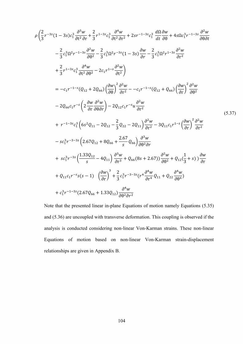
104

𝜌 (2

3𝑟−3𝑠(1 − 3𝑠)𝑐1

3∂3𝑤

∂t2 ∂r+

2

3𝑟1−3𝑠𝑐1

3∂4𝑤

∂t2 ∂r2+ 2𝑠𝑟−1−3𝑠𝑐1

3 𝑑Ω

𝑑𝑡

∂𝑤

∂θ+ 4𝑠Ω𝑐1

3𝑟−1−3𝑠∂2𝑤

∂θ𝜕𝑡

−2

3𝑐1

3Ω2𝑟−1−3𝑠∂2𝑤

∂θ2−

2

3𝑐1

3Ω2𝑟−3𝑠(1 − 3𝑠)∂𝑤

∂𝑟−

2

3𝑐1

3Ω2𝑟1−3𝑠∂2𝑤

∂r2

+2

3𝑟1−3𝑠𝑐1

3∂4𝑤

∂t2 ∂θ2− 2𝑐1𝑟

1−𝑠∂2𝑤

∂t2)

= −𝑐1𝑟−1−𝑠(𝑄12 + 2𝑄66) (

𝜕𝑤

𝜕θ)

2 ∂2𝑤

∂r2− −𝑐1𝑟

−1−𝑠(𝑄12 + 𝑄66) (𝜕𝑤

𝜕r)

2 ∂2𝑤

∂θ2

− 2𝑄66𝑐1𝑟−𝑠 (2

𝜕𝑤

𝜕r

∂2𝑤

∂θ𝜕𝑟) − 2𝑄12𝑐1𝑟

−𝑠𝑢∂2𝑤

∂r2

+ 𝑟−1−3𝑠𝑐13 (6𝑠2𝑄11 − 2𝑄12 −

2

3𝑄22 − 2𝑄11)

∂2𝑤

∂r2− 3𝑄11𝑐1𝑟

1−𝑠 (𝜕𝑤

𝜕r)

2 ∂2𝑤

∂r2

− 𝑠𝑐13𝑟−3−3𝑠 (2.67𝑄12 + 8𝑄66 +

2.67

𝑠𝑄66)

∂3𝑤

∂θ2𝜕𝑟

+ 𝑠𝑐13𝑟−3𝑠 (

1.33𝑄12

𝑠− 4𝑄11)

∂3𝑤

∂r3+ 𝑄66(8𝑠 + 2.67))

∂2𝑤

∂θ2+ 𝑄12(

1

3+ 𝑠) )

𝜕𝑤

𝜕r

+ 𝑄11𝑐1𝑟−𝑠𝑠(𝑠 − 1) (

𝜕𝑤

𝜕r)

3

+2

3𝑐1

3𝑟−3−3𝑠(𝑟4∂4𝑤

∂r4𝑄11 + 𝑄22

∂4𝑤

∂θ4)

+ 𝑐13𝑟−1−3𝑠(2.67𝑄66 + 1.33𝑄12)

∂4𝑤

∂θ2𝜕𝑟2

(5.37)

Note that the presented linear in-plane Equations of motion namely Equations (5.35)

and (5.36) are uncoupled with transverse deformation. This coupling is observed if the

analysis is conducted considering non-linear Von-Karman strains. These non-linear

Equations of motion based on non-linear Von-Karman strain-displacement

relationships are given in Appendix B.

105

5.4 Bending mode vibrations of rotating Stodola’s disc

The lowest out-of-plane mode for the rotating Stodola’s disc is the transverse

mode or it can be named as the bending mode. Transverse vibrations of the rotating

Stodola’s discs rotating about its axis at constant angular speed are studied. It is clear

from the above equations of motion of the transverse vibration that they are not coupled

with displacements of other two directions. Hence, the lowest bending mode can be

treated independently. Higher out-of-plane modes are coupled in terms of

displacements and can be grouped based on the nodal diameters (i.e. n equals to 1, 2...).

The circumferential symmetry of the circular Stodola’s disc about the circumferential

coordinate is considered. Mid-plane transverse direction displacement of the rotating

Stodola’s disc can be written in terms of the assumed shape functions, which is as

follows:

𝑤(𝑟, θ, t) = 𝑊(𝑟) cos 𝑛θ sin𝜔𝑡 (5.38)

where, 𝑊 represents the amplitude of vibration in transverse direction.

For the lowest bending mode (𝑛 = 0), let the amplitude be expressed by the following

polynomial:

𝑊(𝑟) = 𝑛𝑧 ∑𝐶𝑖

𝐼

𝑖=1

𝑟𝑖−1 (5.39)

where I is the maximum number of terms in the polynomial. The constraint function

𝑛𝑧 for the clamped-free annular disc in Equation (5.39) is 𝑟

𝑅0, which is multiplied with

each term. This constraint function is necessary to impose necessary boundary

condition to the disc. For the free-fixed boundary condition, it takes the form of

𝑟

𝑅0− 1.

106

5.4.1 Maximum strain energy and maximum kinetic energy for bending mode

Equation (5.38) is substituted in Equations (5.13) and (5.23) to derive maximum

strain energy and maximum kinetic energy of the rotating disc. Hence, one gets:

(Π𝑟𝑜𝑡)𝑚𝑎𝑥 = ∫ ∫ 𝑐13𝑟−1−3𝑠 (

1

3𝑟𝑄11 (

𝑑2𝑊

𝑑𝑟2)

2𝑅𝑜

𝑅𝑖

2𝜋

0

+2

3𝑄12 (

𝑑2𝑊

𝑑𝑟2) (

𝑑𝑊

𝑑𝑟) +

1

3𝑟𝑄22 (

𝑑𝑊

𝑑𝑟)

2

)𝑟𝑑𝑟 𝑑𝜃

(5.40)

(T𝑟𝑜𝑡)𝑚𝑎𝑥 = 𝜌 𝑐1 ∫ ∫ (1

3𝑟1−3𝑠𝑐1

2Ω2 (𝑑𝑊

𝑑𝑟)2

+ Ω2r3−s 𝑅𝑜

𝑅𝑖

2𝜋

0

+ r1−s𝑊2𝜔2)𝑟𝑑𝑟 𝑑𝜃

(5.41)

Kinetic energy of rotating disc can be seen as the kinetic energy of stationary disc plus

the kinetic energy due to rotational effect. Hence, they are maximized independently to

get the maximum kinetic energy of the rotating Stodola’s disc.

To maximize the energies, it should be noted that maximum values of sin2 𝜔𝑡

and cos2 𝜔𝑡 are considered while deriving Equations (5.40) and (5.41). In Equation

(5.41), terms 1

3𝜌 𝑟2−3𝑠𝑐1

3Ω2 (𝑑𝑊

𝑑𝑟)2

and 𝜌 𝑐1Ω2r3−s describe the work done in bending

due to the centrifugal force generated due to rotational effect, hence these terms should

be added to the maximum strain energy equation. This centrifugal effect generated due

to rotation modifies the stiffness of structure. Based on this fact, Equations (5.40) and

(5.41) are modified and rewritten as follows:

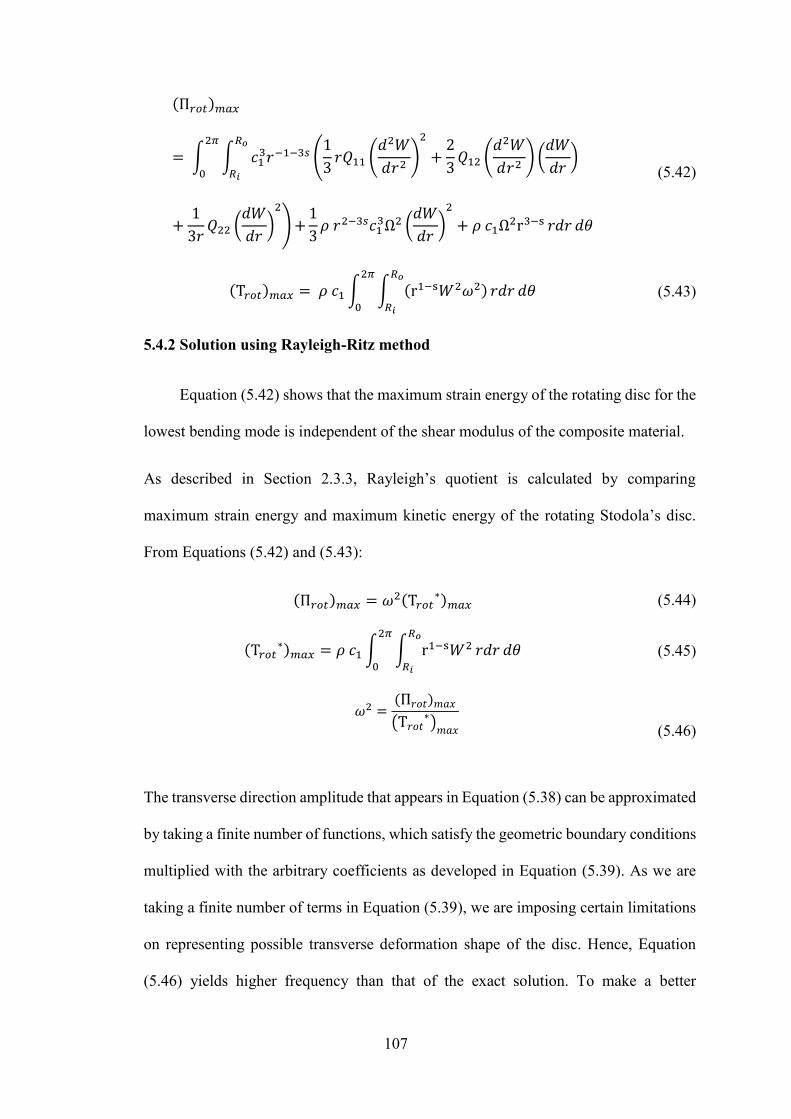
107

(Π𝑟𝑜𝑡)𝑚𝑎𝑥

= ∫ ∫ 𝑐13𝑟−1−3𝑠 (

1

3𝑟𝑄11 (

𝑑2𝑊

𝑑𝑟2)

2

+2

3𝑄12 (

𝑑2𝑊

𝑑𝑟2) (

𝑑𝑊

𝑑𝑟)

𝑅𝑜

𝑅𝑖

2𝜋

0

+1

3𝑟𝑄22 (

𝑑𝑊

𝑑𝑟)2

)+1

3𝜌 𝑟2−3𝑠𝑐1

3Ω2 (𝑑𝑊

𝑑𝑟)2

+ 𝜌 𝑐1Ω2r3−s 𝑟𝑑𝑟 𝑑𝜃

(5.42)

(T𝑟𝑜𝑡)𝑚𝑎𝑥 = 𝜌 𝑐1 ∫ ∫ (r1−s𝑊2𝜔2)𝑅𝑜

𝑅𝑖

2𝜋

0

𝑟𝑑𝑟 𝑑𝜃 (5.43)

5.4.2 Solution using Rayleigh-Ritz method

Equation (5.42) shows that the maximum strain energy of the rotating disc for the

lowest bending mode is independent of the shear modulus of the composite material.

As described in Section 2.3.3, Rayleigh’s quotient is calculated by comparing

maximum strain energy and maximum kinetic energy of the rotating Stodola’s disc.

From Equations (5.42) and (5.43):

(Π𝑟𝑜𝑡)𝑚𝑎𝑥 = 𝜔2(T𝑟𝑜𝑡∗)𝑚𝑎𝑥 (5.44)

(T𝑟𝑜𝑡∗)𝑚𝑎𝑥 = 𝜌 𝑐1 ∫ ∫ r1−s𝑊2

𝑅𝑜

𝑅𝑖

2𝜋

0

𝑟𝑑𝑟 𝑑𝜃 (5.45)

𝜔2 =(Π𝑟𝑜𝑡)𝑚𝑎𝑥

(T𝑟𝑜𝑡∗)𝑚𝑎𝑥

(5.46)

The transverse direction amplitude that appears in Equation (5.38) can be approximated

by taking a finite number of functions, which satisfy the geometric boundary conditions

multiplied with the arbitrary coefficients as developed in Equation (5.39). As we are

taking a finite number of terms in Equation (5.39), we are imposing certain limitations

on representing possible transverse deformation shape of the disc. Hence, Equation

(5.46) yields higher frequency than that of the exact solution. To make a better

108

approximation to estimate the natural frequency of the lowest bending mode,

Rayleigh’s quotient with respect to the arbitrary coefficients is minimized. Hence, one

gets:

𝜕𝜔2

𝜕𝐶𝑖= 0 (5.47)

From Equations (5.46) and (5.47),

𝜕(Π𝑟𝑜𝑡)𝑚𝑎𝑥

𝜕𝐶𝑖− 𝜔2

𝜕(T𝑟𝑜𝑡∗)𝑚𝑎𝑥

𝜕𝐶𝑖= 0 (5.48)

Equation (5.48) gives the set equations which are homogeneous and linear in

𝐶1, 𝐶2, 𝐶3, …. The number of equation obtained from Equation (5.48) is equal to the

number of coefficients in Equation (5.39). These equations can be rewritten in the

matrix form as follows:

([𝐾] − 𝜔2[𝑀])[{𝐶𝑖}] = 0 (5.49)

where, {𝐶𝑖} is the column vector consisting of coefficients. To have non-zero solution,

the determinant of augmented matrix, which consists of the coefficients

𝐶1, 𝐶2, 𝐶3, …must be zero. MAPLE code is developed to calculate the bending mode

natural frequency (𝜔𝑖, 𝑖 = 1,2, …) of rotating Stodola’s disc.

5.4.3 Solution using Finite element method (using ANSYS)

It is important to consider the pre-stressed effectes generated due to rotation of

the Stodola’s disc. It is believed that this effect modifies the overall stiffness of the

structure. Hence, the pre-stressed modal analysis is performed from a linear based

analysis. SOLID 186 elements are considered for the pre-stressed modal analysis.

SOLID 186 element is a higher-order 3-D, 20-node element. It has quadratic

109

displacement behaviour and is well suited to model structures with irregular meshes.

The element has three degrees of freedom at each node that are translation one.

Moreover, the SOLID186 element has stress stiffening and large deflection capabilities.

Large deflection option is turned off during the simulation. The inclusion of large

deflection effects means that ANSYS accounts for changes in the stiffness due to the

change in the shape of the disc.

5.4.4 Example

Consider that the outer radius and the inner radius of Stodola’s disc are 0.5m and

0.1m respectively. The inner thickness of the disc is 0.4m and taper parameter of

Stodola’s disc is taken as 0.861353(i.e. outer thickness of the disc becomes 0.1 m).

Modulus of elasticity and Poisson’s ratio for Structural Steel material are 200 GPa and

0.3 respectively. The clamped-free boundary condition is considered in the analysis.

Consider that the disc is rotating at a constant angular speed of 100 rad/sec.

Four terms are considered in Equation (5.39). Comparison of the two solution methods

explained in sub-sections 5.4.2 and 5.4.3 are given in Table 5.1 as follows:

Solution

method

Lowest bending mode

natural frequency 𝑓3 (Hz)

RR solution 1195.6283

Finite element solution

using ANSYS

(𝑓3)

1194.1

% Difference -0.128

Table 5.1: Comparison of lowest transverse mode natural frequency of Stodola’s disc

rotating at constant angular velocity of 100 rad/sec and beta value of 0.2

110

5.5 Parametric study

The effect of rotational speed on the lowest transverse mode natural frequency is

studied. Note that the Stodola’s disc of taper parameter value 0.861353 has an outer

thickness of 0.1 m and hyperbolic thickness variation along the radial direction. Such a

disc of taper parameter value 0.861353 can be considered as moderately thick disc and

Kirchhoff hypothesis is expected to give closer results. Four number of terms are

considered in the Rayleigh-Ritz polynomial for this disc of outer thickness value 0.1 m.

Parametric study with respect to rotational speed is conducted and presented in Table

5.2 as follows:

5.5.1 Effect of rotational speed on lowest bending mode natural frequency

Rotational speed

(Ω) in

rad/sec

RR solution

in Hz

Finite element

solution in Hz

(using ANSYS)

(𝑓3)

%

Difference

100 1195.6283 1194.1 -0.128

200 1195.8516 1194.3 -0.13

300 1196.2168 1194.6 -0.135

400 1196.7137 1195.0 -0.143

500 1197.3296 1195.6 -0.145

600 1198.0489 1196.2 -0.155

700 1198.8555 1197.0 -0.155

800 1199.7322 1197.9 -0.153

900 1200.6625 1198.9 -0.147

1000 1201.6304 1200.1 -0.128

1499 1206.5828 1207.5 0.076

2000 1211.0613 1217.8 0.553

2499 1214.7147 1230.7 1.3

Table 5.2: Variation of bending mode natural frequency with rotational speed for the

isotropic Stodola’s disc having radius ratio of 0.2

111

From above Table 5.2, it is concluded that effect of rotational speed on the natural

frequency of the lowest transverse mode (i.e. bending mode) is not significant for the

lower rotating speeds. As the gyroscopic couple is neglected in the present analysis,

there are no forward-whirl and backword-whirl frequencies obtained. Hence, increase

in the natural frequency with an increase in rotational speed is solely due to increasing

the stiffness due to centrifugal forces. At higher rotating speed, the gyroscopic effect

should be considered to accurately predict the critical speeds of rotating structures.

112

For orthotropic disc, material properties presented in Table 2.6 are considered.

Geometry of Stodola’s disc made of orthotropic material is considered to the same as

that of isotropic Stodola’s disc analysis presented in sub-section 5.5.1. The effect of

rotational speed on lowest bending mode is studied. The following Table 5.3 shows the

variation of 𝑓4 (in ANSYS) of orthotropic Stodola’s disc rotating at constant rotational

speed for each case.

Rotational speed

(Ω) in

rad/sec

Rotational speed

(Ω) in

rpm

RR solution

in Hz

Finite element

solution in Hz

(using ANSYS)

(𝑓4)

100 954.93 665.7915 638.62

200 1909.86 666.1405 639.01

300 2864.79 666.6692 639.65

400 3819.72 667.3167 640.56

500 4774.65 668.0253 641.72

600 5729.58 668.7432 643.13

700 6684.51 669.4392 644.8

800 7639.44 670.0922 646.71

900 8594.37 670.6931 648.86

1000 9549.30 671.2411 651.25

1499 14314.40 673.3061 666.58

Table 5.3: Variation of bending mode natural frequency with rotational speed for the

orthotropic Stodola’s disc having radius ratio of 0.2

113

5.5.2 Effect of taper parameter on the lowest bending mode natural frequency

The following Figure 5.1 shows the variation of lowest bending mode natural

frequencies of rotating Stodola’s disc with taper parameters. Consider three values of

taper parameters S1, S2 and S3 as 0.861353, 0.609423 and 0.430677 respectively.

These values of taper parameters generate the Stodola’s discs of outer thicknesses 0.1,

0.15 and 0.2 m respectively. Stodola’s disc made of Structural Steel material is

considered here. It is observed that the lowest bending mode natural frequency is

inversely proportional to the taper parameter value of the disc.

Figure 5.1: Variation of natural frequency 𝑓3 of Stodola’s disc with taper parameter

and rotational speed for beta value of 0.2

It is not advisable to study the free vibration response of the discs with lower values of

taper parameter using presented formulation as these generate considerable thickness

1190

1195

1200

1205

1210

1215

1220

1225

1230

1235

1240

0 200 400 600 800 1000 1200 1400 1600

Nat

ura

l fre

qu

ency

f3

(in

Hz)

Rotational speed (in rad/sec)

RR solution for taper parameter S1 RR solution for taper parameter S2

RR solution for taper parameter S3

114

in the transverse direction. The ignorance of transverse shear deformation makes the

present formulation inadequate for the thick discs. It is clear from Table 5.2 that,

Rayleigh-Ritz solutions for rotating discs are in good agreement with the three-

dimensional ANSYS solution.

5.5.3 Effect of degree of orthotropy on natural frequency

A parametric study based on the degree of orthotropy is conducted in this section.

Degree of orthotropy (��) can be defined as the ratio of Young’s Modulus of material in

radial direction to Young’s Modulus in circumferential direction. The value of this ratio

of taken from 0.1 to 10. Recall that the elements of material stiffness matrix consists of

Equations (5.8) to (5.11):

𝑄𝑖𝑗 =

[

𝐸1

1 − 𝑣12𝑣21

𝑣21𝐸1

1 − 𝑣12𝑣210

𝑣21𝐸1

1 − 𝑣12𝑣21

𝐸2

1 − 𝑣12𝑣210

0 0 𝐺12]

(5.50)

Upon simplifying,

𝑄𝑖𝑗 =𝐸1

1 − 𝑣12𝑣21

[

1 𝑣21 0

𝑣21 𝐸2

𝐸10

0 0𝐺12(1 − 𝑣12𝑣21)

𝐸1 ]

(5.51)

Substituting 𝐸1

𝐸2= �� in above Equation (5.51), one gets:

𝑄𝑖𝑗 =𝐸1

1 − ��𝑣212

[

1 𝑣21 0

𝑣21 1

��0

0 0𝐺12(1 − ��𝑣21

2 )

𝐸1 ]

(5.52)

115

The maximum energies given by Equations (5.42) and (5.43) are modified considering

the stiffness elements of Equation (5.52). The variation of frequency factor Ω𝑟𝑜𝑡 =

𝜔 √𝜌 (1 − ��𝑣21

2 )

𝐸1 for the bending mode with the degree of orthotropy is studied. Consider

the Stodola’s disc having radius ratio of 0.2 and taper parameter value of 0.861353. To

study the sole effect of degree of orthotropy on the lowest bending mode natural

frequency, the rotational speed of Stodola’s disc is kept at zero for this analysis. The

following Figure (5.2) shows the stated behaviour of the disc.

Figure 5.2: Variation of frequency parameter with the degree of orthotropy for

Stodola’s disc of beta value of 0.2 and 𝑣21 = 0.3

It is concluded from above Figure 5.2 that the bending mode natural frequency for each

taper parameter of Stodola’s disc decreases due to the decrease in bending stiffness with

the degree of orthotropy.

0

0.5

1

1.5

2

2.5

3

3.5

4

0 1 2 3 4 5 6 7 8 9 10

Freq

uen

cy p

aram

eter

Degree of orthotropy

frequency parameter for S1 frequency parameter for S2

frequency parameter for S3

116

5.6 Conclusion

In this Chapter, the effect of rotational speed on the lowest bending mode natural

frequency is studied based on the linear analysis. Transverse shear effects have been

neglected in the analysis to simplify the mathematical calculations. The clamped-free

boundary condition has been considered throughout this Chapter. Rayleigh-Ritz

method has been employed to calculate the lowest bending mode natural frequency.

Moreover, the effect of degree of orthotropy on bending mode natural frequency is

studied. A summary of observations is given next:

Rayleigh’s quotient for the rotating Stodola’s disc is calculated for the first time

considering the work done by centrifugal forces due to rotational effect.

Accordingly, the total strain energy of the Stodola’s disc was modified.

Overall stiffness of the disc increases and as a result the bending mode natural

frequency increases with the rotational speed.

It is observed that at lower rotating speeds, the increase in the bending mode

natural frequency is not significant.

The bending mode natural frequency of rotating Stodola’s disc decreases with

increase of taper parameter of Stodola’s disc.

117

Chapter 6 Conclusion and future work

6.1 Major Contributions

The major contributions of present study are as follow:

1) The free-vibration response of uniform thickness disc of clamped-free boundary

condition made of orthotropic material is studied based on the three-dimensional

elasticity theory.

2) Effect of damping on natural frequency of the uniform-thickness disc is studied

considering the modal mass participation factor. This procedure leads to better

prediction of damped natural frequency as it accounts for the variable nature of

damping ratios as mode increases.

3) The novel numerical approach based on the classical Rayleigh-Ritz method with

finite-element-like modification is developed to study the free vibration response of

linearly-tapered discs and non-linearly tapered discs of clamped-free boundary

condition and made of isotropic and orthotropic materials.

4) Transverse mode vibrations of rotating Stodola’s disc are investigated using

Rayleigh-Ritz method. Kirchoff hypothesis is considered to reduce the complexity

of the problem. The Rayleigh-Ritz solution is validated with three-dimensional

finite element solution. Moreover, the effect of rotational speed on the lowest

bending mode natural frequency is studied for Stodola’s disc of clamped-free

boundary condition. The effect of degree of orthotropy on lowest bending mode

natural frequency is presented for rotating Stodola’s disc.

5) The effects of taper angle and taper parameter of linearly-tapered disc and non-

linearly-tapered discs on lowest circumferential mode and bending mode natural

frequencies are studied respectively.

118

6.2 Conclusions

The principal conclusions of the present study are as follow:

1) For the uniform-thickness disc made of Graphite-Polymer Composite material, the

circumferential mode natural frequency only depends on the shear modulus of the

material. Further, it is observed that circumferential mode natural frequency of

circular disc is higher than that of the lowest bending mode natural frequency. This

is because of the fact that the circumferential mode involves pure shearing and the

sole component of displacement present is in the tangential direction of the disc

middle surface. This concludes the higher stiffness of the disc in circumferential

mode vibration compared to bending mode vibration. Furthermore, the spacing

between these two frequencies is considerably less in the uniform thickness disc

made of Graphite-Polymer composite material compared to the disc made of

Structural Steel material.

2) It is concluded from the present study that the lowest bending mode natural

frequency increases with Poisson’s ratio. Natural frequencies of modes with one or

higher nodal diameter number increase with Poisson’s ratio. The circumferential

mode natural frequency decreases slightly with increase in Poisson’s ratio. This is

because of reduction of shear modulus and subsequently due to the reduction of

stiffness of the disc in circumferential direction.

3) The Rayleigh-Ritz method with finite-element-like modification allows the use of

lower order polynomial to calculate the lowest in-plane mode and the lowest out-

of-plane mode natural frequencies of linearly-tapered circular disc and Stodola’s

disc of clamped-free boundary condition.

119

4) For linearly-tapered disc of clamped-free boundary condition, the variation of

lowest bending mode natural frequency is higher at higher radius ratios.

5) The lowest in-plane mode natural frequency increases with taper parameter of

Stodola’s disc. Whereas, the lowest bending mode natural frequency has parabolic

variation with taper parameter of Stodola’s disc of clamped-free boundary

condition.

6) The natural frequencies of in-plane mode and out-of-plane mode vibrations increase

with taper angle and radius ratio in the case of linearly-tapered isotropic or

orthotropic disc of clamped-free boundary condition.

7) The lowest bending mode natural frequency of Stodola’s disc of clamped-free

boundary condition increases with the rotational speed because of the fact that

stiffness of the structure increases due to the centrifugal forces generated due to

rotation.

8) The effect of degree of orthotropy on the lowest bending mode natural frequency is

significant at lower values of Young’s modulus ratio of orthotropic material.

120

6.3 Future recommendations

1) The present work can be extended to study the forced vibration response of the

stationary and rotating circular discs.

2) The present work is based on the consideration of linear strains. Von-Karman strain

non-linearity can be considered for non-linear analysis.

3) Coriolis effect may be considered to predict the three-dimensional dynamic

response of Stodola’s disc rotating at high rotational speeds.

4) In practical applications, the thickness of rotating discs is much beyond the limits

of thin plate theory. In such cases, FSDT (First order shear deformation theory) or

higher order shear deformation theory can be considered to have better accuracy in

determining free vibration response of moderately thick discs.

121

Appendix A

Non-linear equations of motion for orthotropic Stodola’s disc rotating at constant speed

are as follows:

𝜌 (𝑟1−𝑠 𝑑Ω

𝑑𝑡 𝑣 + 2𝑟1−𝑠Ω

𝑑 𝑣

𝑑𝑡− 𝑟1−𝑠

∂2u

∂t2+ 𝑟1−𝑠Ω2𝑢

+ 𝑟2−𝑠Ω2)

= −𝑟−𝑠(1 − 𝑠)𝑄11

𝜕𝑢

𝜕𝑟− 𝑟1−𝑠𝑄11

∂2u

∂r2

+ 𝑢𝑟−𝑠−1(𝑄22 + 𝑠𝑄12) − 𝑄66𝑟−𝑠−1

∂2u

∂θ2

− 𝑟−𝑠−1𝜕𝑤

𝜕θ

∂2w

∂θ𝜕𝑟(𝑄66 + 𝑄12)

− 2𝑄66𝑟−𝑠−1

𝜕𝑤

𝜕r

∂2w

∂θ2

+1

2𝑟−𝑠 (

𝜕𝑤

𝜕r)2

(𝑄12 − (1 − 𝑠)𝑄11)

− 𝑟1−𝑠𝑄11

𝜕𝑤

𝜕r

∂2w

∂𝑟2

+1

2𝑟−𝑠−2 (

𝜕𝑤

𝜕θ)2

(𝑄22 + (𝑠 + 1)𝑄12)

+ 𝑟−𝑠−1𝜕𝑣

𝜕θ(𝑄22 + 𝑄66 + 𝑠𝑄12)

− 𝑟−𝑠∂2𝑣

∂θ𝜕𝑟(𝑄66 + 𝑄12)

122

𝜌 (− 𝑟1−𝑠 𝑑Ω

𝑑𝑡 (𝑢 + 𝑟) − 2𝑟1−𝑠Ω

∂𝑢

∂𝑡− 𝑟1−𝑠

∂2𝑣

∂t2+ 𝑟1−𝑠Ω2𝑣)

= −𝑄22𝑟−𝑠−1

∂2𝑣

∂θ2− 𝑄66𝑟

−𝑠∂𝑣

∂𝑟(1 − 𝑠) − 𝑟1−𝑠𝑄66

∂2𝑣

∂r2

− 𝑄66𝑣𝑟−𝑠−1(𝑠 − 1) − 𝑄66𝑟−𝑠−1

∂𝑤

∂𝑟

∂𝑤

∂θ(1 − 𝑠) − 𝑄66𝑟

−𝑠∂𝑤

∂θ

∂2𝑤

∂r2

− 𝑟−𝑠∂𝑤

∂𝑟

∂2𝑤

∂θ∂𝑟(𝑄12 + 𝑄66) − 𝑟−𝑠−1

∂𝑢

∂θ(𝑄22 + (1 − 𝑠)𝑄66)

− 𝑄22𝑟−𝑠−2

∂𝑤

∂θ

∂2𝑤

∂θ2− 𝑟−𝑠

∂2𝑢

∂θ∂r(𝑄12 + 𝑄66)

123

𝜌 (2

3𝑟−3𝑠(1 − 3𝑠)𝑐1

3∂3𝑤

∂t2 ∂r+

2

3𝑟1−3𝑠𝑐1

3∂4𝑤

∂t2 ∂r2+ 2𝑠𝑟−1−3𝑠𝑐1

3 𝑑Ω

𝑑𝑡

∂𝑤

∂θ+ 4𝑠Ω𝑐1

3𝑟−1−3𝑠∂2𝑤

∂θ𝜕𝑡

−2

3𝑐1

3Ω2𝑟−1−3𝑠∂2𝑤

∂θ2−

2

3𝑐1

3Ω2𝑟−3𝑠(1 − 3𝑠)∂𝑤

∂𝑟−

2

3𝑐1

3Ω2𝑟1−3𝑠∂2𝑤

∂r2

+2

3𝑟1−3𝑠𝑐1

3∂4𝑤

∂t2 ∂θ2− 2𝑐1𝑟

1−𝑠∂2𝑤

∂t2)

= −𝑐1𝑟−1−𝑠(𝑄12 + 2𝑄66) (

𝜕𝑤

𝜕θ)

2 ∂2𝑤

∂r2− −𝑐1𝑟

−1−𝑠(𝑄12 + 𝑄66) (𝜕𝑤

𝜕r)

2 ∂2𝑤

∂θ2

− 2𝑐1𝑟−𝑠(𝑄12 + 𝑄66)

𝜕𝑤

𝜕r

∂2𝑣

∂θ𝜕𝑟− 2𝑄66𝑐1𝑟

−𝑠 (𝜕𝑤

𝜕θ

∂2𝑣

∂r2+ 2

𝜕𝑤

𝜕r

∂2𝑤

∂θ𝜕𝑟)

− 2𝑄12𝑐1𝑟−𝑠𝑢

∂2𝑤

∂r2− 𝑟−1−3𝑠𝑐1

3 ((6𝑠2𝑄11 − 2𝑄12 −2

3𝑄22 − 2𝑄11)

∂2𝑤

∂r2)

− 2𝑄12𝑐1𝑟−𝑠

𝜕𝑣

𝜕θ

∂2𝑤

∂r2− 2𝑄22𝑐1𝑟

−2−𝑠𝑢∂2𝑤

∂θ2− 2𝑄22𝑐1𝑟

−𝑠−2 (𝜕𝑤

𝜕θ

∂2𝑣

∂θ2+

𝜕𝑣

𝜕θ

∂2𝑤

∂θ2)

− 2𝑄11𝑐1𝑟1−𝑠 (

𝜕𝑤

𝜕r

∂2𝑢

∂r2+

𝜕𝑢

𝜕r

∂2𝑤

∂r2) − 𝑐1𝑟

−1−𝑠(𝑄12 + 𝑄66) − 2𝑄12𝑐1𝑟−1−𝑠

𝜕𝑢

𝜕r

∂2𝑤

∂θ2

− 2𝑄66𝑐1𝑟−1−𝑠 (

𝜕𝑤

𝜕r

∂2𝑢

∂θ2+ 2

𝜕𝑢

𝜕θ

∂2𝑤

∂θ𝜕𝑟− 2𝑣

∂2𝑤

∂θ𝜕𝑟)3𝑄22𝑐1𝑟

−3−𝑠 (𝜕𝑤

𝜕θ)

2 ∂2𝑤

∂θ2

− 3𝑄11𝑐1𝑟1−𝑠 (

𝜕𝑤

𝜕r)

2 ∂2𝑤

∂r2− 𝑠𝑐1

3𝑟−3−3𝑠 (2.67𝑄12 + 8𝑄66 +2.67

𝑠𝑄66)

∂3𝑤

∂θ2𝜕𝑟

+ 𝑠𝑐13𝑟−3𝑠 (

1.33𝑄12

𝑠− 4𝑄11)

∂3𝑤

∂r3

+ 𝑐13𝑟−3−3𝑠(𝑄12(6𝑠2 + 6𝑠 + 1.33) + 𝑄22(2𝑠 + 1.33) + 𝑄66(8𝑠 + 2.67))

∂2𝑤

∂θ2

− (8𝑄66 + 4𝑄12)𝑐1𝑟−1−𝑠

∂2𝑤

∂θ𝜕𝑟

𝜕𝑤

𝜕r

𝜕𝑤

𝜕θ+ 𝑐1𝑟

−2−𝑠(𝑠 + 1)(𝑄12 + 2𝑄66)𝜕𝑤

𝜕r(𝜕𝑤

𝜕θ)

2

+ 2𝑄66𝑐1(1 + 𝑠)𝑟−1−𝑠𝜕𝑤

𝜕θ

𝜕𝑣

𝜕r+ 2𝑐1𝑟

−1−𝑠(𝑠𝑄12 + 𝑄66)𝜕𝑣

𝜕θ

𝜕𝑤

𝜕r

+ 2𝑐1𝑟−𝑠(𝑄11(𝑠 − 1) − 𝑄12)

𝜕𝑢

𝜕r

𝜕𝑤

𝜕r+ 2𝑐1𝑟

−2−𝑠(𝑄66(𝑠 + 1) − 𝑄22)𝜕𝑤

𝜕θ

𝜕𝑢

𝜕θ

− 2𝑄66𝑐1𝑟−2−𝑠(1 + 𝑠)𝑣

𝜕𝑤

𝜕θ+ 2𝑐1

3𝑟−2−3𝑠(𝑄12 (𝑟2𝑠+1

𝑐12 𝑠𝑢 + 𝑠 + 3𝑠2) + 𝑄12(

1

3

+ 𝑠) )𝜕𝑤

𝜕r+ 𝑄11𝑐1𝑟

−𝑠𝑠(𝑠 − 1) (𝜕𝑤

𝜕r)

3

+2

3𝑐1

3𝑟−3−3𝑠(𝑟4∂4𝑤

∂r4𝑄11 + 𝑄22

∂4𝑤

∂θ4)

+ 𝑐13𝑟−1−3𝑠(2.67𝑄66 + 1.33𝑄12)

∂4𝑤

∂θ2𝜕𝑟2

124

Appendix B

Three-dimensional Rayleigh-Ritz solution for the uniform-thickness disc of clamped-

free boundary condition is presented in Chapter 2. Presented results are validated by

comparing them to the Rayleigh-Ritz solution obtained using series comprising of

orthogonally-generated polynomial functions derived by Kim and Dickinson [22] and

the 2D exact solution [46].

In this example, the uniform-thickness disc of clamped-free boundary condition made

of Structural Steel material is considered. The values for Young’s modulus and

Poisson’s ratio are considered as 200 GPa and 0.3 respectively for this material. Density

is considered as 7850 𝑘𝑔/𝑚3. Beta value of the disc is considered as 0.1, which is the

ratio of inner radius to outer radius of the disc. Thickness of the disc is taken as 0.15 m.

The inner radius and outer radius of the circular annular disc are taken as 0.2 m and 2

m. The following Table B.1 shows the comparison of presented results with Rayleigh-

Ritz solution obtained using series comprising of orthogonally-generated polynomial

functions derived by Kim and Dickinson.

Solution method Beta

value

Numbers of nodal diameter and nodal circle (𝑛, 𝑠)

(0,0) (1,0) (2,0) (3,0) (4,0)

Present

0.1

41.2609 30.1554 48.7213 110.6195 193.5625

polynomial 𝐼 = 𝑄 = 3,𝐽 = 𝑃 = 4

𝐼 = 𝐾 = 𝑄 = 4 and 𝐽 = 𝐿 = 𝑃 = 2

Kim &

Dickinson [22] 38.6330 31.7256 51.2819 113.5071 199.064

2D Exact [46]

38.5619 28.6252 51.2336 113.0421 -

Polynomial

0.5

𝐼 = 𝑄 = 3,𝐽 = 𝑃 = 3 𝐼 = 𝐽 = 𝐾 = 𝐿 = 𝑃 = 𝑄 = 3

Present

119.1250 125.5368 136.4365 168.4583 229.4701

Kim &

Dickinson [22] 118.7307 121.1556 134.046 169.2168 233.3408

2D Exact [46]

118.5119 121.2468 134.0096 168.6512 -

Table B. 1: Comparison of natural frequencies of uniform-thickness annular C-F disc

125

In above Table B.1, (𝑛, 𝑠) represents the nodal diameter number and nodal circle

number respectively. For zero nodal diameter number and zero nodal circle value, the

results are compared with that of literature for the lowest transverse mode vibration.

The boundary condition taken at inner radius is clamped and at outer radius the

boundary condition considered is free. It is shown that the presented data are in good

agreement with the 2D exact solutions for natural frequencies of transversely vibrating

uniform annular plates derived using Bessel’s functions by Vogel and Skinner [46].

Three-dimensional Rayleigh-Ritz solution for clamped-free circular annular disc,

presented in this thesis may be useful to validate the results obtained using 2-D plate

theories.

The natural frequency results obtained using Rayleigh-Ritz method with finite-element-

like modification are presented in Chapter 3. Validation is conducted by comparing the

natural frequencies of linearly-tapered disc of small taper angle with that of uniform-

thickness disc of comparable thickness.

Consider the linearly-tapered disc of clamped-free boundary condition and made

of the same material as that of the uniform-thickness disc, considered for the validation

in above Table B.1. The linearly-tapered disc with small taper angle of 0.1592 degree

is considered with beta value of 0.1. This way, outer thickness of the linearly-tapered

disc becomes 0.14 m. Thicknesses of uniform-thickness disc are considered as 0.15 m

and 0.14 m.

The following Table B.2 shows the comparison of natural frequency results of

linearly-tapered disc with small taper angle with the results of uniform-thickness

circular annular disc of clamped-free boundary condition.

126

Mode type

Linearly-

tapered disc

with taper

angle of

0.1592

degree

(ℎ𝑖 = 0.14)

Number

of

divisions

Uniform-

thickness disc

of ℎ = 0.15

Uniform-

thickness disc of

ℎ = 0.14

Lowest

circumferential

mode natural

frequency

(in Hz)

72.9074

𝐾 = 𝐿 = 1

5

71.4508

𝐾 = 𝐿 = 4

74.3620

𝐾 = 𝐿 = 4

Lowest bending

mode natural

frequency

(in Hz)

39.8818

𝐼 = 𝐽 = 2,

𝑃 = 𝑄 = 2

61

41.2609

𝐼 = 𝑄 = 3,

𝐽 = 𝑃 = 4

38.6090

𝐼 = 𝑄 = 3,

𝐽 = 𝑃 = 4

Table B. 2: Comparison of natural frequencies of linearly-tapered annular C-F disc

From above Table B.2, it is concluded that the natural frequencies of the lowest

in-plane mode and the lowest out-of-plane mode vibration changes slightly with small

taper angle. Here, for the disc with thicknesses 0.14 m and 0.15 m, it is observed that

the circumferential mode natural frequency is higher than that of the frequency of

vibration in lowest bending mode.

127

Appendix C

The selection of number of divisions considered in Chapter 3 to calculate natural

frequencies of in-plane and out-of-plane vibration modes of linearly-tapered disc is

described below:

Results presented in Figure 3.3, Figure 3.6, Figure 3.8, Table 3.1, Table 3.2 and

Table 3.3 are calculated considering the following number of divisions and the order of

polynomial.

Results Mode type Beta value

Number of

divisions

Order of

polynomial

Figure 3.3

In-plane

0.2 5

𝐾 = 𝐿 = 1 0.25 3

0.3 2

Figure 3.6 Out-of-plane

0.2 3 𝐼 = 𝑄 = 1

and

𝐽 = 𝑃 = 2

0.25 2

Figure 3.8 In-plane

0.2 5

𝐾 = 𝐿 = 1 0.25 3

0.3 2

Table 3.1 Out-of-plane 0.2 6 𝐼 = 𝑄 = 1

and

𝐽 = 𝑃 = 2

Table 3.2 Out-of-plane 0.25 4

Table 3.3 Out-of-plane 0.3 3

Table C. 3: Selection of number of divisions to calculate the natural frequencies

of linearly-tapered disc

128

The selection of number of divisions considered in Chapter 4 to calculate natural

frequencies of in-plane and out-of-plane vibration modes of Stodola’s disc is as follows:

Results presented in Table 4.1 and Table 4.2 are calculated considering the

following number of divisions and the order of polynomial.

Results Mode type

Beta

value

Taper

parameter

Number

of

divisions

Order of

polynomial

Table 4.1

In-plane

0.2

-

4 𝐾 = 𝐿 = 1

Table 4.2

Out-of-

plane

0.2

0.861353 3 𝐼 = 𝑄 = 2

and

𝐽 = 𝑃 = 2

0.609423 2

0.430677 2

0.29203 2

0.178747 2

Table C. 4: Selection of number of divisions to calculate the natural frequencies

of Stodola’s disc

129

Bibliography

[1] J. Obuchowski, A. Wylomanska, and R. Zimroz, “Vibration Engineering and

Technology of Machinery,” Mech. Mach. Sci., vol. 23, pp. 401–410, 2015.

[2] D. J. Thompson and C. J. C. Jones, “A Review of the Modelling of Wheel/Rail Noise

Generation,” J. Sound Vib., vol. 231, no. 3, pp. 519–536, 2000.

[3] “http://www.walter-tools.com/en-

gb/industry_solutions/aerospace/engine/pages/turbine_disk.aspx.” .

[4] “https://www.performanceonline.com/1937-42-ford-car-disc-brake-conversion-kits/.” .

[5] W. Weaver, S. P. Timoshenko, and D. H. Young, Vibration Problems in Engineering.

John Wiley & Sons, 1990.

[6] A. Love, A treatise on the Mathematical Theory of Elasticity. New York: Dover

Publications, 1944.

[7] H. Deresiewicz and R. Mindlin, “Axially symmetric flexural vibrations of a circular

disk,” Am. Soc. Mech. Eng. J. Appl. Mech., vol. 22, pp. 86–88, 1955.

[8] V. Kunukkasseril and S. Venkatesan, “Free Vibration of Layered Circular Plates,” J.

Sound Vib., vol. 60, no. 4, pp. 511–534, 1978.

[9] P. Guruswamy and T. Y. Yang, “A sector finite element for dynamic analysis of thick

plates,” J. Sound Vib., vol. 62, no. 4, pp. 505–516, 1979.

[10] T. Irie, G. Yamada, and K. Takagi, “Natural Frequencies of Thick Annular Plates,” J.

Appl. Mech., vol. 49, no. September 1982, pp. 633–638, 2016.

[11] K. M. Liew, Y. Xiang, C. M. Wang, and S. Kitipornchai, “Flexural Vibration of Shear

Deformable Circular and Annular Plates on Ring Supports,” Comput. Methods Appl.

130

Mech. Eng., vol. 110, pp. 301–315, 1993.

[12] J. So and A. W. Leissa, “Three-Dimensional Vibrations of Thick Circular and Annular

Plates,” J. Sound Vib., vol. 209, no. 1, pp. 15–41, 1998.

[13] J. Kang, “Free vibration analysis of shallow spherical dome by three-dimensional Ritz

method,” J. Vib. Control, pp. 1–14, 2014.

[14] D. Zhou, F. T. K. Au, Y. K. Cheung, and S. H. Lo, “Three-dimensional vibration

analysis of circular and annular plates via the Chebyshev–Ritz method,” Int. J. Solids

Struct., vol. 40, no. 12, pp. 3089–3105, 2003.

[15] C. Il Park, “Frequency Equation for the In-plane Vibration of a Clamped Circular

Plate,” J. Sound Vib., vol. 313, no. 1–2, pp. 325–333, 2008.

[16] S. Bashmal, R. Bhat, and S. Rakheja, “In-plane free vibration analysis of an annular

disk with point elastic support,” Shock Vib., vol. 18, pp. 627–640, 2011.

[17] S. Bashmal, R. Bhat, and S. Rakheja, “In-plane free vibration of circular annular

disks,” J. Sound Vib., vol. 322, no. 1–2, pp. 216–226, 2009.

[18] C. H. Huang and Y. . Chen, “Vibration Analysis for Piezoceramic Circular Plates with

V-Notches Part 1:Theory,” J. Mech., vol. 30, no. 6, pp. 603–609, 2014.

[19] C. Sridhar and K. P. Rao, “Large Deformation Finite Element Analysis of Laminated

Circular Composite plates,” Comput. Struct., vol. 54, no. 1, pp. 59–64, 1995.

[20] K. Gupta, S. . Singh, V. Tiwari, S. Takkar, R. Dev, and A. Rai, “Vibration Analysis of

Fiber Reinforced Composite Discs,” in 9th IFToMM International Conference on

Rotor Dynamics, Mechanisms and Machine Science, 2015, vol. 21, no. July, pp. 1665–

1675.

131

[21] Q. Wang, D. Shi, Q. Liang, and F. Ahad, “A Unified Solution for Free In-plane

Vibration of Orthotropic Circular, Annular and Sector Plates with General Boundary

Conditions,” Appl. Math. Model., vol. 40, pp. 9228–9253, 2016.

[22] C. S. Kim and S. M. Dickinson, “On the Lateral Vibration of Thin Annular and

Circular Composite Plates Subject to Certain Complicating Effects,” J. Sound Vib.,

vol. 130, no. 3, pp. 363–377, 1989.

[23] C. Prasad, R. K. Jain, and S. R. Soni, “Axisymmetric vibrations of circular plates of

linearly varying thickness,” J. Appl. Math. Phys., vol. 23, no. 6, pp. 941–948, 1972.

[24] U. S. Gupta and R. LaL, “Vibrations and Buckling of Parabolically Tapered Circular

Plates,” Indian J.ournal pure Appl. Math., vol. 10, no. 3, pp. 347–356, 1979.

[25] S. R. Soni and C. L. Amba-rao, “Axisymmetric Vibrations of Annular Plates of

Variable Thickness,” J. Sound Vib., vol. 38, no. 4, pp. 465–473, 1975.

[26] J. Kirkhope and G. J. Wilson, “Vibration and stress analysis of thin rotating discs using

annular finite elements,” J. Sound Vib., vol. 44, no. 4, pp. 461–474, 1976.

[27] C. A. Mota Soares and M. Petyt, “Finite Element Dynamic Analysis of Practical

Discs,” J. Sound Vib., vol. 61, no. 4, pp. 547–560, 1978.

[28] T. A. Lenox and H. D. Conway, “An exact, closed form, solution for the flexural

vibration of a thin annular plate having a parabolic thickness variation,” J. Sound Vib.,

vol. 68, no. 2, pp. 231–239, 1980.

[29] J. N. Reddy and C. L. Haung, “Nonlinear axisymmetric bending of annular plates with

varying thickness,” Int. J. Solids Struct., vol. 17, no. 8, pp. 811–825, 1981.

[30] B. Singh and V. Saxena, “Axisymmetric Vibration of a Circular Plate with Double

Linear Variable Thickness,” J. Sound Vib., vol. 179, no. 5, pp. 879–897, 1995.

132

[31] W. H. Duan, S. T. Quek, and Q. Wang, “Generalized hypergeometric function

solutions for transverse vibration of a class of non-uniform annular plates,” J. Sound

Vib., vol. 287, no. 4–5, pp. 785–807, 2005.

[32] U. S. Gupta, R. Lal, and S. Sharma, “Vibration analysis of non-homogeneous circular

plate of nonlinear thickness variation by differential quadrature method,” J. Sound

Vib., vol. 298, no. 4–5, pp. 892–906, 2006.

[33] D. Sheen and K. . Viswanathan, “Free Vibration of Layered Circular Cylindrical Shells

of Variable Thickness Using Spline Function Approximation,” Indian J. Eng. Mater.

Sci., vol. 16, no. December, pp. 433–448, 2009.

[34] H. Lamb and R. V. Southwell, “The Vibrations of a Spinning Disk,” Proc. R. Soc.

London, vol. 99, no. 699, pp. 272–280, 2016.

[35] J. Nowinski, “Nonlinear Transverse Vibrations of a Spinning Disk,” Trans. ASME, pp.

72–78, 1964.

[36] Y. C. S. Barasch, “On the Vibration of a Rotating Disk,” Am. Soc. Mech. Eng. Appl.

Mech., vol. 39, pp. 1143–1144, 1972.

[37] N. Baddour, “A Modelling and Vibration Analysis of Spinning Disks,” University of

Toronto, 2001.

[38] A. Khoshnood and M. A. Jalali, “Normal oscillatory modes of rotating orthotropic

disks,” J. Sound Vib., vol. 314, no. 1–2, pp. 147–160, 2008.

[39] H. R. Hamidzadeh, “In-plane free vibration and stability of rotating annular discs,”

Proc. Inst. Mech. Eng. Part K J. Multi-body Dyn., vol. 216, no. 4, pp. 371–380, 2002.

[40] S. Dousti and M. Abbas Jalali, “In-Plane and Transverse Eigenmodes of High-Speed

Rotating Composite Disks,” J. Appl. Mech., vol. 80, no. 011019, pp. 1–7, 2012.

133

[41] ANSYS Inc., “ANSYS Mechanical APDL Element Reference,” 2013.

[42] I. Chowdhury and S. P. Dasgupta, “Computation of Rayleigh Damping Coefficients

for Large Systems,” Electron. J. Geotech. Eng., vol. 8, no. 0, 2003.

[43] M. Hyer, “Stress analysis of fiber-reinforced composite materials.” 1998.

[44] S. S. Rao, The Finite Element Method in Engineering, Third Edit. Butterworth-

Heinemann publications, 1999.

[45] “http://www.geaviation.com/commercial/engines/genx/.” .

[46] S. M. Vogel and D. W. Skinner, “Natural Frequencies of Transversely Vibrating

Uniform Annular Plates,” J. Appl. Mech., no. 2010, pp. 926–931, 1965.