1/8/2017

1

TWO-DAY DYADIC DATA ANALYSIS

WORKSHOPRandi L. Garcia

Smith College

UCSF January 9th and 10th

@RandiLGarcia RandiLGarcia

Smith professor of:• Psychology• Statistical and Data

Sciences

A little about me…

What about you?

1/8/2017

2

Workshop Materials on GitHub

>Find the workshop schedule and data examples here:

https://randilgarcia.github.io/website/workshop/schedule.html

>Download ALL materials, including R-code, here:

https://github.com/RandiLGarcia/2day-dyad-workshop

DAY 1• Definitions and Nonindependence• Data Structures• The Actor-Partner Interdependence Model (APIM)• Generalized Mixed Modeling (i.e., for discrete outcomes)

1/8/2017

3

Definitions: Distinguishability

• Can all dyad members be distinguished from one another based on a meaningful factor?

• Distinguishable dyads• Gender in heterosexual couples

• Patient and caregiver

• Race in mixed race dyads

All or Nothing

• If most dyad members can be distinguished by a variable (e.g., gender), but a few cannot, then can we say that the dyad members are distinguishable?

• No, we cannot!

6

1/8/2017

4

Indistinguishability

• There is no systematic or meaningful way to order the two scores

• Examples of indistinguishable dyads• Same-sex couples

• Twins

• Same-gender friends

• Mix of same-sex and heterosexual couples

• When all dyads are hetero except for even one couple!

It can be complicated…

• Distinguishability is a mix of theoretical and empirical considerations.

• For dyads to be considered distinguishable:1. It should be theoretically important to make such a distinction between members.

2. Also it should be shown that empirically there are differences.

• Sometimes there can be two variables that can be used to distinguish dyad members: Spouse vs. patient; husband vs. wife.

8

1/8/2017

5

Types of Variables

• Between Dyads • Variable varies from dyad to dyad, BUT within each dyad all individuals have the same

score

• Example: Length of relationship

• Called a level 2, or macro variable in multilevel modeling

B

A

B

A A

A

AB

A

B

1/8/2017

6

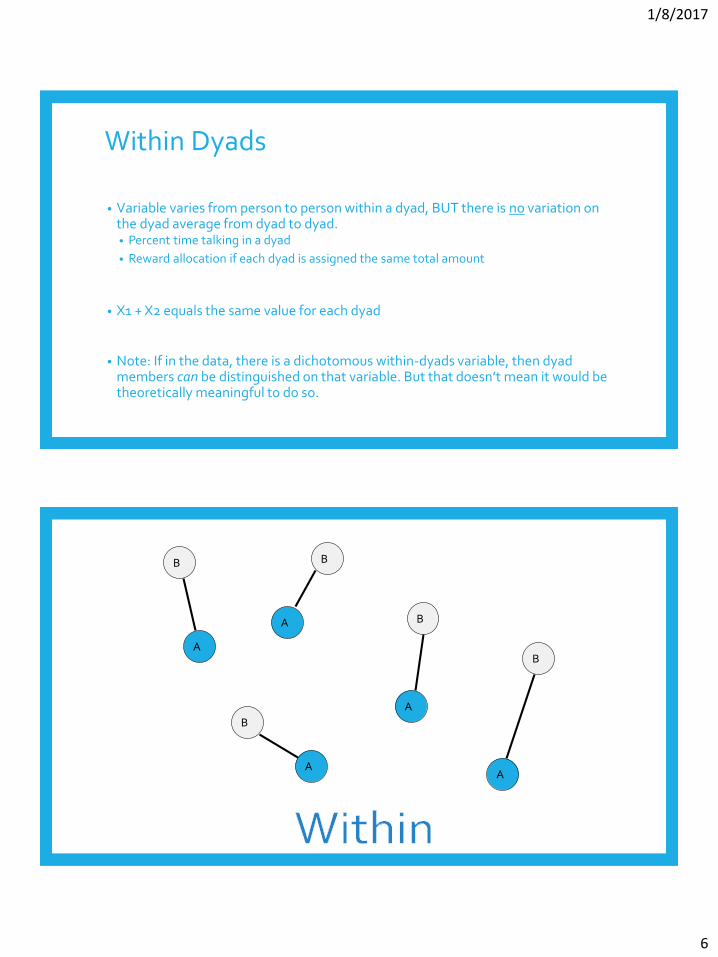
Within Dyads

• Variable varies from person to person within a dyad, BUT there is no variation on the dyad average from dyad to dyad. • Percent time talking in a dyad

• Reward allocation if each dyad is assigned the same total amount

• X1 + X2 equals the same value for each dyad

• Note: If in the data, there is a dichotomous within-dyads variable, then dyad members can be distinguished on that variable. But that doesn’t mean it would be theoretically meaningful to do so.

B

B

B

B B

A

AA

A

A

1/8/2017

7

Mixed Variable

• Variable varies both between dyads and within dyads.

• In a given dyad, the two members may differ in their scores, and there is variation across dyads in the average score.• Age in married couples

• Lots-o personality variables

• Most outcome variables are mixed variables.

It can be complicated…

Can you think of a variable that can be between-dyads, within-dyads, or mixed across different samples?

14

1/8/2017

8

TYPES OF DYADIC DESIGNS

15

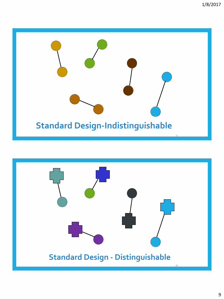
Standard Dyadic Design

• Each person has one and only one partner.

• About 75% of research with standard dyadic design

• Examples: Dating couples, married couples, friends

16

1/8/2017

9

Standard Design-Indistinguishable17

Standard Design - Distinguishable 18

1/8/2017

10

The One-with-Many Design

• All partners have the same role with the focal person

• For example, students with teachers or workers with managers

19

Round-Robin Design

• Social Relations Model (SRM)

• Examples: Team or family members rating one another

20

1/8/2017

11

DATA STRUCTURES

Illustration of Data Structures: Individual

1/8/2017

12

Illustration of Data Structures: Individual

Illustration of Data Structures: Dyad

1/8/2017

13

Illustration of Data Structures: Dyad

Illustration of Data Structures: Pairwise

1/8/2017

14

Illustration of Data Structures: Pairwise

R DEMOThen break! Then more demo…

1/8/2017

15

NONINDEPENDENCE IN DYADS

Negative Nonindependence

• Nonindependence is often defined as the proportion of variance explained by the dyad (or group).

• BUT, nonindependence can be negative…variance cannot!

• This is super important

• THE MOST IMPORTANT THING ABOUT DYADS!

1/8/2017

16

How Might Negative Correlations Arise?

Examples

• Division of labor: Dyad members assign one member to do one task and the other member to do another. For instance, the amount of housework done in the household may be negatively correlated.

• Power: If one member is dominant, the other member is submissive. For example, self-objectification is negatively correlated in dyadic interactions.

Effect of Nonindependence

• Consequences of ignoring clustering classic MLM• Effect Estimates Unbiased

• For dyads especially• Standard Errors Biased

• Sometimes too large

• Sometimes too small

• Sometimes hardly biased

1/8/2017

17

Direction of Bias Depends on

1. Direction of Nonindependence• Positive

• Negative

2. Is the predictor a between or within dyads variable? (or somewhere in between: mixed)

Effect of Ignoring Nonindependence on Significance Tests

Positive Negative

Between Too liberal Too

conservative

Within Too

conservative Too liberal

1/8/2017

18

What Not To Do!

• Ignore it and treat individual as unit

• Discard the data from one dyad member and analyze only one members’ data

• Collect data from only one dyad member to avoid the problem

• Treat the data as if they were from two samples (e.g., doing an analysis for husbands and a separate one for wives)• Presumes differences between genders (or whatever the distinguishing variable is)

• Loss of power

What To Do

• Consider both individual and dyad in one analysis!1. Multilevel Modeling

2. Structural Equation Modeling

1/8/2017

19

Traditional Model: Random Intercepts

𝑦𝑖𝑗 = 𝑏0𝑗 + 𝑏1𝑗𝑋1𝑖𝑗 + 𝑒𝑖𝑗

𝑏0𝑗 = 𝑔00 + 𝑔01𝑍1𝑗 + 𝑢0𝑗

𝑏1𝑗 = 𝑔10

• 𝑖 from 1 to 2, because there are only 2 people in each “group”.

• 𝑋1𝑖𝑗 is a mixed or within variable, and 𝑍1𝑗 is a between variable.

• Note 𝑏0𝑗 is the common intercept for dyad 𝑗 which captures the nonindependence.

• Works well with positive nonindependence, but not negative.

Micro level

Macro level

Alternative Model: Correlated Errors

𝑦1𝑗 = 𝑏0 + 𝑏1𝑗𝑋11𝑗 + 𝑒1𝑗

𝑦2𝑗 = 𝑏0 + 𝑏1𝑗𝑋12𝑗 + 𝑒2𝑗

𝑏1𝑗 = 𝑔10

• 𝜌 is the correlation between 𝑒1𝑗 and 𝑒2𝑗, the 2 members’ residuals (errors).

• Note 𝑏0 is now the grand intercept

• Works well with positive nonindependence AND negative.

Micro level

Macro level

𝜌 called “rho”

1/8/2017

20

R DEMO

ACTOR-PARTNER INTERDEPENDENCE

MODEL (APIM)

1/8/2017

21

Actor-Partner Interdependence Model (APIM)• A model that simultaneously estimates the effect of a person’s own variable (actor

effect) and the effect of same variable but from the partner (partner effect) on an outcome variable

• The actor and partner variables are the same variable from different persons.

• All individuals are treated as actors and partners.

Data Requirements

• Two variables, X and Y, and X causes or predicts Y

• Both X and Y are mixed variables—both members of the dyad have scores on X and Y.

• Example• Dyads, one a patient with a serious disease and other being the patient’s spouse. We are

interested in the effects of depression on relationship quality

1/8/2017

22

Actor Effect

• Definition: The effect of a person’s X variable on that person’s Y variable• the effect of patients’ depression on patients’ quality of life

• the effect of spouses’ depression on spouses’ quality of life

• Both members of the dyad have an actor effect.

Partner Effect

• Definition: The effect of a person’s partner’s X variable on the person’s Y variable• the effect of patients’ depression on spouses’ quality of life

• the effect of spouses’ depression on patients’ quality of life

• Both members of the dyad have a partner effect.

1/8/2017

23

Distinguishability and the APIM

• Distinguishable dyads • Two actor effects

• An actor effect for patients and an actor effect for spouses

• Two partner effects• A partner effect from spouses to patients and a partner effect from

patients to spouses

Distinguishable Dyads

• Errors not pictured (but important)

• The partner effect is fundamentally dyadic. A common convention is to refer to it by the outcome variable. Researcher should be clear!

1/8/2017

24

Indistinguishable Dyads

• The two actor effects are set to be equal and the two partner effects are set to be equal.

Nonindependence in the APIM

• Green curved line: Nonindependence in Y• Red curved line: X as a mixed variable (r cannot be 1 or -1)• Note that the combination of actor and partner effects explain some of the

nonindependence in the dyad.

1/8/2017

25

R DEMO

TEST OF DISTINGUISHABILITY

1/8/2017

26

Test of Distinguishability

• Advantages of Treating Dyad Members as Indistinguishable• Simpler model with fewer parameters

• More power in tests of actor and partner effects

• Disadvantages of Treating Dyad Members as Indistinguishable• If distinguishability makes a difference, then the model is wrong.

• Sometimes the focus is on distinguishing variable and it is lost.

• Some editors or reviewer will not allow you to do it.

Test of Distinguishability

• Four ways that dyads can be distinguishable1. Intercepts (main effect of distinguishing variable)

2. Actor effects

3. Partner effects

4. Error variances

1/8/2017

27

Test of Distinguishability

• Two runs:

• Distinguishable (either interaction or two-intercept, results are the same)• Different Actor and Partner Effects

• Main Effect of Distinguishing Factor

• Heterogeneity of Variance (CSH)

• Indistinguishable (4 fewer parameters)• Same Actor and Partner Effects

• No Main Effect of Distinguishing Factor

• Homogeneity of Variance (CSR)

Test of Distinguishability

• Run using ML, not REML

• Note the number of parameters• There should be 4 more than for the distinguishable run.

• Note the -2LogLikelihood (deviance)

• Subtract the deviances and number of parameters to get a c2 with 4df

• Conclusion: If c2 is not significant, then the data are consistent with the null hypothesis that the dyad members are indistinguishable. If however, c2 is significant, then the data are inconsistent with the null hypothesis that the dyad members are indistinguishable (i.e., dyad members are distinguishable in some way).

1/8/2017

28

R DEMO

BINARY AND COUNT OUTCOME VARIABLES

Generalized Linear Mixed Models

1/8/2017

29

Generalized Linear Models

• In general we wrap the response variables in a link function (log, logit, probit, identity, etc.).

• For example • A logistic regression is a generalized linear model making use of a logit link function.

• A log-linear of Poisson regression is a generalized linear model making use of a log link function.

• A regression model is a generalized linear model making use of an “identity” link function—the response is multiplied by 1.

Logistic Regression Review

• DV is dichotomous• probability of belonging to group 1: 𝑃1• probability of belonging to group 0: 𝑃0 = 1 − 𝑃1.

• There are only two choices!

1/8/2017

30

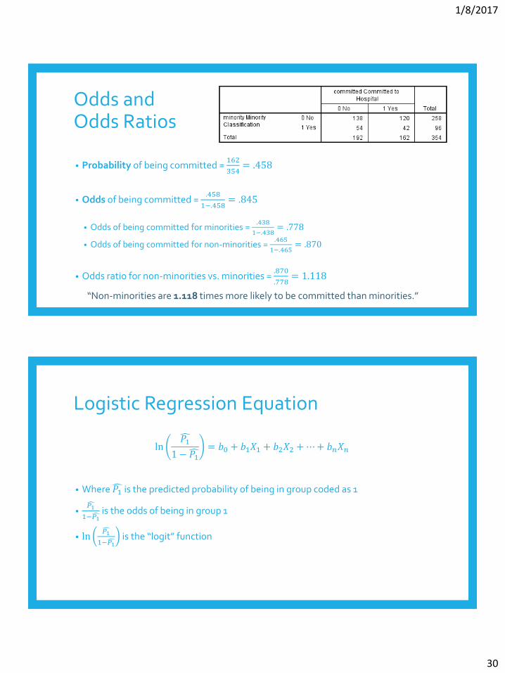
Odds and Odds Ratios

• Probability of being committed = 162

354= .458

• Odds of being committed = .458

1−.458= .845

• Odds of being committed for minorities = .438

1−.438= .778

• Odds of being committed for non-minorities = .465

1−.465= .870

• Odds ratio for non-minorities vs. minorities = .870

.778= 1.118

“Non-minorities are 1.118 times more likely to be committed than minorities.”

Logistic Regression Equation

ln 𝑃1

1 − 𝑃1= 𝑏0 + 𝑏1𝑋1 + 𝑏2𝑋2 +⋯+ 𝑏𝑛𝑋𝑛

• Where 𝑃1 is the predicted probability of being in group coded as 1

• 𝑃1

1− 𝑃1is the odds of being in group 1

• ln 𝑃1

1− 𝑃1is the “logit” function

1/8/2017

31

Logistic Regression Equation

ln 𝑃1

1 − 𝑃1= 𝑏0 + 𝑏1𝑋1 + 𝑏2𝑋2 +⋯+ 𝑏𝑛𝑋𝑛

• The b’s are interpreted as the increase in log-odds of being in the target group for 1-unit increase in X.

• Exp(b) is the increase in odds for 1 unit increase in X—this works out to the odds ratio between X = a and X = a+1.

Log-Linear (Poisson) Regression Equation

• Used when the response variable is a count (e.g., number of cigarettes smoked per day).

ln 𝑌 = 𝑏0 + 𝑏1𝑋1 + 𝑏2𝑋2 +⋯+ 𝑏𝑛𝑋𝑛

• Where 𝒀 is the response vairable

• 𝒍𝒏 𝒀 is the “log” link function

• 𝒃𝟏 is interpreted as the increase in log-Y for every increase in 𝑿𝟏

• Exp(𝒃𝟏) is interpreted in the usual way—as in the general linear model.

1/8/2017

32

Generalized Mixed Linear Models

• Generalized linear models• In general we wrap the response in a link function (log, logit, probit, identity, etc.).

• Generalized Mixed Linear Models• Do the same, include a link function that is appropriate for your response, but then

include random effects in the model.

• “Mixed” refers to the mixture of fixed and random effects in the model.

• We’ll fit these models with the lme4 package in R, specifically, the glmer() function.

Generalized Estimating Equations (GEE)

• Nonindependence treated as a “nuisance” to be removed; no statistical tests of nonindependence

• Can be extended to:• Binomial outcome

• Multinomial outcome (Categories: home/work/leisure)

• Count data (Poisson, negative binomial)

• Can also be used for continuous outcomes (normal distribution)

• Fit these models with the gee package in R, specifically, the gee() function.

1/8/2017

33

R DEMO