during the ngendei experiment1 · the mss sensors are four teledyne model s-750 seis-mometers...

8. PRELIMINARY ANALYSIS OF OCEAN-BOTTOM AND SUB-BOTTOM MICROSEISMIC NOISEDURING THE NGENDEI EXPERIMENT1

Richard G. Adair, John A. Orcutt, and Thomas H. Jordan, Scripps Institution of Oceanography2

ABSTRACT

Simultaneous measurements of ambient microseismic noise at and below the seafloor are compared over the band0.2-7.0 Hz using data collected during the Ngendei Seismic Experiment. Borehole data were collected with a triaxial setof seismometers which rested undamped at the bottom of DSDP Hole 595B, 124 m sub-bottom, 54 m within basementrock. Ocean-bottom data were collected with six 4-component ocean-bottom seismographs (OBSs) deployed at dis-tances ranging from 0.5 to 30 km from the borehole. Noise spectra of displacement power density at both borehole andocean-bottom sites typically displayed the microseism peak between 0.15 and 0.25 Hz. Vertical-component spectra felloff from this peak at 60-80 dB/decade with various peaks superposed. The peaks suggest that the noise consisted ofseismic waves trapped in the seafloor. Vertical ocean-bottom and borehole noise levels are nearly identical at the mi-croseism peak, on the order of I08 nm2/Hz, but OBS values exceed Marine Seismic System (MSS) values by 10 dB ormore at frequencies between 0.5 and 7 Hz. In the borehole, horizontal noise levels were essentially the same as the verti-cal-component levels. At the ocean bottom, horizontal noise levels exceed vertical levels between 0.4 and 7 Hz, but havecomparable values at the microseism peak. Ocean-bottom pressure measurements of ambient noise are comparable toother published measurements; Ngendei values are on the order of I04 Pa2/Hz at the microseism peak. Leg 91 noisemeasurements contrast with those from the prototype MSS deployment during DSDP Leg 78B, when levels at a proxi-mate seafloor site exceeded borehole levels by 10-30 dB over the entire band of valid comparisons (0.16-2.2 Hz). Be-tween 0.3 and 2.2 Hz, Leg 78B borehole levels were greater than those of Leg 91 by 10-20 dB. Leg 78B spectra did notdisplay any obvious peaks other than the microseism peak, where high vertical-component coherence was observed be-tween pairs of OBSs separated by 0.7 km. At the quietest land sites, vertical-component noise levels at the microseismpeak are 10-30 dB lower than those measured in the borehole during Leg 91. At higher frequencies, the noise levelsmeasured in the borehole still exceed those of the quietest land sites, but are lower than at average land sites.

INTRODUCTION

Poor sensitivity and high levels of instrumental noiseplagued the earliest generation of ocean-bottom seismo-graphs (OBSs) employed during the 1960s. Most of theseefforts were funded by the Advanced Research ProjectsAgency (ARPA) of the Air Force through Project VE-LA Uniform to facilitate the seismic discrimination ofnuclear explosions (Prentiss and Ewing, 1963; Bradnerand Dodds, 1964; Latham and Sutton, 1966; Lathamand Nowroozi, 1968; Schneider and Backus, 1964; andSchneider et al., 1964). It was hoped that ambient ocean-bottom noise levels would be substantially lower than atland sites, but in fact they were found to be comparableor higher. This result, coupled with the logistical diffi-culty of employing OBSs, led to the eventual abandon-ment of this research effort. The current revitalizationof OBS usage is due primarily to recent developments insemiconductor technology and hardware, particularly indigital recording techniques, and they have been used pri-marily to investigate seafloor structure through refrac-tion experiments. Several problems still arise, however,from the nearly ubiquitous blanket of sediments at theocean bottom. OBSs must contend with poor coupling

Menard, H. W., Natland, J., Jordan, T. H., Orcutt, J. A., et al., Init. Repts. DSDP,91: Washington (U.S. Govt. Printing Office).

2 Addresses: (Adair, Orcutt) Institute of Geophysics and Planetary Physics (A-025),Scripps Institution of Oceanography, La Jolla, CA 92093, (Adair, present address: RockwellHanford Operations, Energy Systems Group, P.O. Box 800, Richland, WA 99352); (Jordan,present address) Department of Earth, Atmospheric, and Planetary Sciences, MassachusettsInstitute of Technology, Cambridge, MA 02139.

and signal "ringing" caused by unconsolidated sediments(Sutton et al., 1981), as well as with the inherent diffi-culty of observing important converted shear phases(Spudich and Orcutt, 1980). A final difficulty, which isthe primary interest of this chapter, is the high ambientnoise levels at the ocean bottom, thought to be due tonoise propagation as low-order trapped modes confinednear the interface between the seafloor and the oceanbottom. The high noise levels may be mitigated by em-placing seismometers in the more rigid material underly-ing the sediments. Accordingly, interest has been kin-dled in the use of marine borehole seismographs as analternative to OBSs.

Several Deep Sea Drilling Project (DSDP) legs havebeen devoted to "oblique refraction" studies employingcommercially available seismometer systems in boreholes(Stephen et al., 1980, 1983). Because of high instrumen-tal noise levels, these data are not suitable for ambientnoise analysis. Two marine borehole systems have recent-ly been developed to answer these needs: the ocean sub-bottom seismometer (OSS) of the Hawaii Institute ofGeophysics and the Marine Seismic System (MSS) fund-ed by the Defense Advanced Research Projects Agency(DARPA). A detailed description of the OSS and its op-erational use is given in the Leg 88 part of this volumeand in Duennebier and Blackinton (1983).

The feasibility of the MSS design and installation pro-cedure were successfully tested with the deployment of aprototype borehole instrumentation package in Hole 395Aduring DSDP Leg 78B in late March 1981 (Hyndman,Salisbury et al., 1984). Noise data and refraction signals

357

R. G. ADAIR, J. A. ORCUTT, T. H. JORDAN

were recorded on the prototyped two vertical-compo-nent seismometers over a 26-hr, operational period. Si-multaneous measurements of vertical-component noiseat a nearby seafloor site were higher than the boreholelevels by at least 10 dB between 0.16 and 2.2 Hz (Adairet al., 1984). Encouraged by the Leg 78B results, re-searchers attempted to deploy the complete MSS ensem-ble on DSDP Leg 88, but were thwarted by foul weatherand drilling problems (Duennebier et al., Leg 88 part ofthis volume). The MSS deployment was rescheduled forLeg 91, originally a DSDP transit leg between Welling-ton, New Zealand, and Papeete, Tahiti.

The Ngendei Experiment, which includes DSDP Leg91, was designed to answer several outstanding ques-tions regarding the generation and propagation of mi-croseismic noise and the relative characteristics of seis-mic signals at and below the seafloor. In addition to theMSS, the experiment employed an array of six OBSs atvarious distances from the drill site. This chapter presentsa preliminary analysis of the Leg 91 seismic data regard-ing the relative character and levels of microseismic noiseat and below the seafloor.

MARINE SEISMIC SYSTEM DESCRIPTION

Marine Seismic System

Only the salient features of the MSS operations andseismic instrumentation will be considered here. Detaileddescriptions of the MSS and its operational use are foundelsewhere in this volume (Harris et al.; Adair, Harris, etal., this volume).

When fully operational, the MSS comprises a bore-hole sensor package connected by coaxial cable to anuntended ocean-bottom recording system. The boreholepackage and a companion shipboard recording console,referred to here as the Teledyne system, were developedby Teledyne-Geotech. The ocean-bottom recording sys-tem and its shipboard counterpart, referred to as Gouldsystems, were developed by Gould, Inc. Global MarineDevelopment Corporation built a carriage for transport-ing the borehole package to the seafloor at the bottomend of the drillstring. The Naval Civil Engineering Lab-oratory in Port Hueneme, CA, designed and tested asubmerged mooring which facilitates the installation andrecovery of the ocean-bottom recording system.

The MSS data used in this paper are transcriptions ofthe original data obtained from DARPA's Center for Seis-mic Studies in Alexandria, Virginia.

MSS InstrumentationThe instrumentation is housed in a 600.6-cm-long pres-

sure vessel of outside diameter 20.3 cm. The instrumen-tation includes seismic sensors, accelerometers, and in-ternal pressure and temperature monitors. Above thepressure vessel is a 343.9-cm-long cable terminator unit,and below it a 43.8-cm-long impact tip. The cable termi-nator incorporates cable-isolating and holelock mecha-nisms.

The MSS sensors are four Teledyne model S-750 seis-mometers configured as a triaxial set (two orthogonalhorizontals and one vertical) and a redundant backup

vertical component. The backup sensor is located 175.5cm below the primary vertical sensor. Output from thethree primary sensors is filtered in midperiod (0.05-10 s)and short-period (0.05-2 s) bands whereas output fromthe backup sensor is passed through the short-periodband only. The resultant seven data streams are thendigitized and transmitted to the recording devices via co-axial cable. For convenience, the sensors and data chan-nels are labeled in subsequent discussion. The horizon-tal sensors are X and Y, and the primary and backupverticals are Z and B, respectively. The prefixes "S" and"M" will refer to the passband of a particular channel.

MSS Recording Systems

The MSS data are collected either on two shipboardsystems employed for diagnostic checkout and recordingredundancy or on an ocean-bottom recording unit. TheGould systems differ vastly from the Teledyne system indigitizing scheme and postdigitizing processing method.Briefly, the Teledyne system samples the data after low-passing them, whereas the Gould systems convolve thedata with a digital low-pass filter after sampling them.The Gould data are initially sampled at an extremelyhigh rate to insure that the fall-off of the instrument re-sponse prevents high-frequency aliasing, and are thenresampled at the desired rate.

Teledyne Shipboard Recorder

Data destined for the shipboard Teledyne system aresampled, amplified at one of four gains (× 1, × 8, × 32,and × 128), and represented as 14-bit integers augmentedby a 2-bit gain code. Each datum is separately ampli-fied, thereby achieving a 21-bit dynamic range with 14-bit resolution. Midperiod data are routinely digitized at4 sample/s, and the short-period data at 40 sample/s,although either of the short-period vertical channels maybe sampled at 80 sample/s by excluding the other.

Gould Shipboard and Ocean-Bottom Recorders

Data transmitted to the ocean-bottom recorder andits shipboard counterpart are represented with a deltamodulator encoding technique. The encoded streams aretransmitted to the recording unit where they are digitallyconvolved with a low-pass, zero phase-shift filter. Thefilter amplitude response is nearly flat below 15°7o of theultimate Nyquist frequency, and thereafter falls at ap-proximately 750 dB/decade. The low-passed digital dataare then resampled at their proper rates and buffered totape with timing and system status information. Midpe-riod data are recorded at a rate of 4 sample/s, and theshort-period data at 40 sample/s. Details of the sam-pling technique and the low-pass filter are given else-where in this volume. The resultant digital data in prin-ciple have 24-bits of both dynamic range and resolution.

The Gould ocean-bottom recording system employs20 tape drives to achieve a 45-day maximum operatingperiod. Power is provided by two battery packs. Each ofthe packs and the data-processing electronics is housedin separate aluminum spheres. The three spheres andvarious hydroacoustic instruments are mounted on analuminum framework. A sediment-penetrating flange rim-

358

SEAFLOOR SEISMIC NOISE

ming the framework bottom secures the recorder pack-age on the seafloor. The flange is bound by magnesium-alloy bolts, which corrode, allowing detachment of thesuperstructure and aiding recovery of the recorder.

MSS Instrument Responses

Figure 1A shows the instrument responses of the MSSsystems. The dashed lines at high frequencies depict theeffect of the Gould low-pass filter. In the absence of thislow-pass filter, the mid-period response is peaked at ap-proximately 1.2 Hz and falls off at 40 and 150 dB/dec-ade towards lower and higher frequencies, respectively.The short-period response is peaked at approximately 15Hz and declines gently toward lower and higher frequen-cies at 40 and 45 dB/decade, respectively. The Gouldlow-pass filter falls at approximately 750 dB/decade be-yond 75% of the Nyquist frequencies.

OCEAN-BOTTOM SEISMOGRAPH DESCRIPTION

The six OBSs are modifications of the four-compo-nent, digital event-recorders described by Moore et al.(1981). The most important modifications incorporatedby the Ngendei OBSs are an increased memory capacityand a seismograph response which emphasizes frequen-cies below 1 Hz. Both of these changes were necessitatedby the needs of earthquake recording. Orcutt et al. (thisvolume) provide a complete description of the OBS in-strumentation employed on the Ngendei Experiment; wesummarize it here.

The OBS sensors are a 1-Hz triaxial set of velocity-transducer seismometers, the Mark Products Inc. modelLr4-3D, and an omnidirectional piezoelectric hydrophone,the Ocean and Atmospheric Sciences Inc. model E-2PD.The seismometers are configured as two orthogonal hori-

zontals and a vertical. For convenience in later discus-sion, the vertical, two horizontal, and hydrophone chan-nels will be labeled Z, X, Y and H, corresponding toOBS data channels 1 through 4, respectively.

A gimbaled mounting corrects, to within 1°, seismom-eter tilts of up to 15° from the vertical. The orientationsof the horizontal components are not directly determinedand must be inferred from, for example, particle motionstudies of seismic refraction shots. The seismic sensorsand electronics are housed in a buoyant aluminum spheremounted on a disposable tripod. A collar of syntacticfoam enhances overall buoyancy. Acoustic communica-tion with the OBS tending ship makes it easier to locatethe capsule and monitor its state of health. Explosivebolts, detonated either by acoustic command or by sched-ule, free the sphere to float to the surface for recovery.

Sensor outputs are amplified, bandpassed, sampled128 times per second with a 12-bit word, and continu-ously stored with gain and timing information in a cycli-cally overwritten buffer. Buffer lengths of approximately13 and 58 s were used during the Ngendei Experiment.The data are buffered to avoid the mechanical shakingand electrical transients caused by recorder operation.Recording proceeds either when a triggering criterion ismet or at scheduled times.

Trigger status and channel gains are determined fromaverages of the digital data. Event triggers are estab-lished with a comparison criterion of short-term andlong-term averages of vertical-component data. A chan-nel^ gain is updated at regular intervals and changedonly then if the long-term average of that channePs out-put falls outside preset bounds of a few least-significantbits. The gain is constrained to be a power of two be-tween 1 and 512, and to change only in a single, 6-dB

>CD

Eα>oCO

αenQ

1 0 8

1 0 6

10

1 0 2

10°

~ A

_

—

-

1//i

1 Mill

MSS, short period

y

/

/ (

fjS \ midperiod£r i\

sf Λ/ / . \St ' \

/ » \/ ' \

/ i \j \Gould i \filter ] \

i ^i 11111in i 11M iin

_

N

Gouldi filter

s —

iii

i

\ii

Ji

-

i i i i i mi

10" 1 0 u 10'

Frequency (Hz)

10c

10*-

Refraction

Teleseismic

Hydrophone

1 I 1 1 1 ( 1 1 1 I I I I I I I I I I Illl

10'

10"

10-3

10-5

10" 1 0 u 10'

Frequency (Hz)

Figure 1. Displacement responses of (A) Marine Seismic System (MSS) and (B) ocean-bottom seismograph (OBS) instrumentation used during theNgendei Experiment. A. The Gould MSS midperiod and short-period responses differ from the Teledyne responses by the low-pass digital filter,shown with dashed lines. B. OBS seismometer and hydrophone responses. Two responses were available for the OBSs.

359


step (a factor of two in amplitude). Because this gain-ranging scheme operates over time scales on the order ofminutes, the gain is essentially fixed during an event, sothat the dynamic range is only 12 bits, with 12-bit reso-lution.

Bandpass filters for the data streams include a re-sponse-shaping stage which reduces the dynamic rangeoccupied by ambient noise. Acoustic and seismic noise,which fall sharply with frequency from a peak near 0.2Hz, may be compensated for with responses emphasiz-ing high frequencies over low. On the other hand, thetriggering algorithm is more sensitive to teleseisms if lowerfrequencies are emphasized, because teleseisms are typi-cally depleted in high frequencies. To meet these variedneeds, two responses for the seismic channels, shown inFigure IB, were employed. The hydrophone response wasnot altered for teleseismic deployments.

OPERATIONS

Figure 2 charts a select chronology of operations andevents. The events of the Ngendei Experiment are conve-niently segregated into three phases according to whetheror not the Gould ocean-bottom recorder was in use.These three phases also roughly demark periods duringwhich the tending ships Glomar Challenger and Melvillewere or were not present. Challenger was responsible forinstallation of the MSS sensors and seafloor recorder,and Melville conducted MSS support operations, sitesurveys, and instrumentation recovery as well as all OBSoperations. The presence of the ship is of concern be-cause microseismic noise measurements are severely con-taminated by ship-generated noise in the frequency banddiscussed here. Ships were absent only during the sec-ond phase.

The 20-day-long first phase included site selections,borehole drilling, instrumentation deployment, and a re-fraction experiment. The second phase comprised a 40-day period of untended earthquake and noise recording.The instrumentation was recovered during the final phase.

Figures 3 and 4 show the MSS borehole site and theOBS locations throughout the Ngendei Experiment. TheMSS site is computed relative to the best satellite esti-mates of Challenger^ positions. Octagons centered onellipses depict computed OBS locations (octagons) andtheir 95% confidence bounds (ellipses) based on least-squares modeling of satellite and acoustic ranging data(Creager and Dorman, 1982). Diamonds denote OBSdrop points estimated from either satellite navigation orMelville radar ranging of Challenger. Capsules are re-ferred to by the first two letters of their names and a nu-meral denoting the deployment number. Tables 1 and 2list the particulars of each OBS, including range and az-imuth from the borehole site, response type and pre-event buffer length.

During the first phase, four of the six OBSs wereplaced in pairs 0.6-0.7 km to the north and southwest ofthe borehole (Figure 3A) for refraction signal recording,and the other two 25-30 km to the east-northeast (Fig-ure 3B) for triggered earthquake recording. All OBSs re-corded noise at various regular intervals. Five distinctrefraction lines were shot.

The second phase began with the redeployment ofthe OBSs in a triangular array and installation of theMSS ocean-bottom recorder and its recovery mooring.Two of the OBSs formed 25-km legs at approximate rightangles to the south and east of the MSS site (Figure 4A).The four other capsules were clustered within 3 km tothe west and north of the MSS borehole (Figure 4B).

1. BIP deploymenta. BIP-1b. BIP-2

2. Shipboard recordinga. Teledyneb. Gould

3. BPP deploymenta. Operationsb. BPP deploymentc. BPP operationald. Data collection

4. BPP recoverya. Operationsb. Data recording

TeledyneGould

c. IRR redeployment

5. Refraction lines

m—4H-HH

44- I f

H 11—+- -H-l

-II-

10 12 14Jj-

February 198324 26March 1983

Figure 2. Chronology of events during the Ngendei Experiment pertinent to the noise study. Coordinated Universal Time (CUT) data aregiven along the bottom axis, with a break between mid-February 1983 and late March 1983, when the teleseismic experiment tookplace and noise samples were recorded by each OBS at 24-hr, intervals. See text for explanation.

360


23.815°S

23.825

0

km

'0.5

JJ\LYI

I

A

KA1

^ * ^ SU1

-

Hole 595B

23.92°S -

23.95 -

165.535 165.525°W 165.79 165.76°W

Figure 3. Locations of the MSS and six OBSs during the first phase of the Ngendei Experiment. See text for explanation of symbols. A. Config-uration of the four capsules which recorded refraction signals (Juan, Karen, Lynn, and Suzy). B. Configuration of the two OBSs which con-currently recorded teleseismic signals in a triggered mode (Janice and Phred).

23.8°S

24.1

A

-

-

-

~^o le 595B

JU3 0

-

0SU2

10

km

23.81 °S

23.82

B

-

-

0

i

A

LY2

I

6

km

KA2

(

1i

PH3

1

-

JA3

Hole 595B

165.6 165.3°W 165.55 165.53 °W

Figure 4. Locations of the MSS and OBSs during the second phase of the Ngendei Experiment. See text for explanation of symbols. A. MSS and 2farthest OBSs. B. MSS and 4 nearest OBSs.

Table 1. OBS locations and characteristics during the Ngendei Experiment, first phase.

OBSsite

JAIJA2JU1KAILY1PHISU1

Lat. (°S)

23.9339823.9361223.8202423.8173323.8207723.9418223.81737

Long. (°W)

165.78653165.76627165.53244165.52758165.53115165.76130165.52745

Deployed21

From

024:0626032:0455029:1104029:0102030:1124023:0604030:0039

To

029:0715034:0815040:0535040:0807041:0817038:0850041:0556

Depth(m)

5704571756185612560356765612

Range,azimuth

(km,°)

29.18, 24527.44, 2420.62, 2920.56, 3520.47, 292

27.29, 2410.56, 353

Responsetype

TeleseismicTeleseismicRefractionRefractionRefractionTeleseismicRefraction

Bufferlength

(s)

58581313135813

Deployment dates in Julian days, year 1983.Reference site is MSS location: 23.82233° South, 165.52683° West. Azimuth is clockwise from North.

361


Table 2. OBS locations and characteristics during the Ngendei Experiment, second phase.

ORSsite

JA3JU3KA2LY2C

PH2SU2

Lat. (°S)

23.8182324.0453123.8093923.8123023.8239423.85997

Long. (°W)

165.52574165.53030165.54157165.55120165.53820165.29674

Deployed21

From

036:1433042:1124042:2142043:1357040:2045041:2247

To

081:1520081:1100082:0600082:1040082:0950081:0531

Depth(m)

560555795593550355445654

Range,azimuth

(km,°)

0.47, 1424.80, 181

2.08, 3142.72, 2941.17, 261

23.77, 100

Responsetype

TeleseismicTeleseismicTeleseismicTeleseismicTeleseismicTeleseismic

Bufferlength

(s)

581358131358

j* Deployment dates in Julian days, year 1983.b Reference site is MSS location: 23.82233° South, 165.52683° West. Azimuth is clockwise from North.c Drop location.

The OBSs recorded daily noise samples and triggeredevents.

Melville recovered the OBSs and the MSS ocean-bot-tom recorder during the final phase. It was discoveredthat the MSS recorder had ceased operations approxi-mately two days after deployment because of a waterleak in one of its battery spheres. Following a brief ship-board recording period, the mooring was redeployed withthe load of the ocean-bottom recorder replaced by a con-crete clump anchor. The instrumentation package wasleft in Hole 595B.

DATA

The following describes the recovered data and vari-ous instrument malfunctions which rendered some ofthese data unsuitable for analysis. Figures 5-7 schemati-cally inventory the noise data.

OBS Data

A total of 1420 noise events were obtained from theOBSs; over half were simultaneous with MSS data, andmost were recorded simultaneously by at least two cap-sules. Noise data were regularly recorded by the OBSsthroughout the experiment. In particular, all capsulesrecorded noise samples at GMT midnight during the fi-nal phase. However, 70% of the OBS noise samples wereoriginally scheduled as seismic refraction events. Thesesamples were the serendipitous result of MSS deploy-ment delays, which forced a drastic rescheduling of therefraction experiment, and of refraction shots which de-tonated late or not at all.

During the first phase of the Ngendei Experiment,four OBS data channels were defective. The gain-rangermalfunctioned in OBS Juan channels Y and H and OBSLynn channel X, resulting in amplified noise amplitudesthat often exceeded the digital word size ("clipped"). OBSJanice channel H suffered a periodic transient signal atintervals of one second.

Only two OBSs were defective during the second phase.The digitizer of OBS Janice channel Z could not set bit3 in addition to the persistent transient of its channel H.Progressive tape head misalignment on OBS Juan ren-dered data recorded after 25 February 1983 inaccessibleby playback instrumentation.

MSS Data

Totals of 119.5, 83.25, and 43.25 hr. of data were re-covered from the Teledyne and Gould shipboard and

Janice

Juan

Karen

_ynn

Phred

Suzy

iiiiiiiiπiiHiiiniiiiiiiiiiiiiiiiiiiiiiiiiiiiiiiiii

II i nim II

II I Him II

II•II•I i

iiiiiiiiiiiiiiiiiiiiiiiiiiiiiiiiiiiii II iiiiiiiiiiiiii inn iiiiiiiii mi mini i iiiiiiiiiiiiiiiiiiiuii

II•II•I i

24 28January February

Figure 5. Chart of noise data available for analysis before the MSS be-gan recording. The OBSs recorded discrete events, shown as verti-cal ticks. CUT date is given along the bottom axis, and capsulenames on left.

ocean-bottom recorders, respectively. Most of the datawere recorded aboard ship over the six-day period im-mediately following sensor emplacement in the borehole,when 114.25 and 70.5 hr. of data were obtained by theTeledyne and Gould systems. All of Refraction Line 5and most of the outbound leg of Line 4 were recordedsimultaneously by the MSS and OBSs. The missed out-bound portion of Line 4, referred to as Line 6, was re-corded only by the MSS at the very end of phase 1, asthe OBSs were being redeployed for the teleseismic ex-periment of phase 2.

MSS data were recorded continuously except for in-terruptions for maintenance or because the system mal-functioned. The most notable malfunction was the totalfailure of the ocean-bottom recording system approxi-mately two days after its deployment. In addition, MSSsensor Y malfunctioned throughout the experiment andyielded no usable data in either the mid- or short-periodbands.

Gould channel SZ, the primary short-period vertical-component channel, was not recorded during most of

362


Janice

Juan

Karen 1

Lynn

Phred

Suzy

Teledyne

Gould

III 1

III 1

1 1 1

1

1 1

1 1

1 1 1

1 III

II III 1

1

1 1

II 1

1

i i

1 1

1

1

1

1

1 1 1 1 1 II

mini

•

•UH

1

1

1 1 1

1 1 1

II Illl

1 1

7February

Figure 6. Noise samples recorded at about the start of MSS data re-cording. The MSS systems recorded continuously during the inter-vals shown with horizontal sediments bounded by vertical lines.MSS recording system and OBS names identified along the left.

Janice

Juan

Karen

Lynn

Phred

Suzy

Teledyne

Gould

I l• II I

II I Illl I I II II

I l l l -HI—H

H H 1—H—I h

10February

11

Figure 7. Noise samples recorded during the latter portion of the firstphase of MSS operations. See caption of Figure 6 for explanation.MSS recording systems and OBS names identified along the left.

the shipboard periods of phases 1 and 3 because it suf-fered radio-frequency interference. Also, a Gould elec-tronics bay in the borehole package which processed chan-nel MZ and initiated calibrations failed at the start ofthe second phase and never resumed operations. Tele-dyne channel MZ, of course, was not affected by thismalfunction.

Quality

Data quality and valid frequencies of microseismicnoise measurement were assessed with both time- andspectral-domain criteria. In particular, power density andcoherence estimates were computed in the manner de-scribed by Welch (1967). Spectra are obtained from de-meaned, nonoverlapping data segments tapered with anormalized Hanning window using a mixed-radix FastFourier Transform algorithm (Singleton, 1969) which doesnot require power-of-two data lengths. Stable spectralestimates are then formed from averages of cross- andauto-spectra. Spectra are normalized so that the totalpower per Nyquist-frequency bandwidth is equal to thetime-domain variance, which essentially folds the energyof the negative frequencies into that of the positive.

Figures 8 and 9 show a typical example of multichan-nel MSS data from the Teledyne and Gould systems, re-spectively, recorded during the shipboard recording peri-od. (Plot scales were chosen to show background noiselevels, with the result that large-amplitude signals ap-pear clipped in this figure.) Y-sensor malfunction is evi-dent from both figures. Note that Gould channel SZ(Fig. 9) is disabled, as explained earlier. The high-fre-quency content of Teledyne and Gould short-period sig-nals is mostly ship-generated by Challenger.

Proper representation of the data was investigated bycomputing relative timing and amplitudes between thetwo recording systems with cross-correlations and linearregressions of corresponding channels (Fig. 10). Typi-cally, data from all short-period and mid-period Gouldchannels led the corresponding Teledyne data by 15 or16 samples and were approximately 5.5 times greater inamplitude rather than 8 times, as we could expect fromtheir different dynamic ranges (24 and 21 bits, respec-tively); the consequence is a 3 dB uncertainty in spectralestimates. Comparisons of data timing with independenttime code (WWV) written adjacent to Teledyne data onstrip-charts indicate that Gould's timing is in error. Tele-dyne sensor calibrations (Fig. 11) of properly function-ing channels are within their expected norms by less than4 dB, suggesting that Gould amplitudes are in error.However, the calibration loop excludes portions of thetotal seismograph circuitry so this discrepancy cannotbe verified. The departure of the MY and SY calibra-tions from the norms further demonstrates sensor mal-function. Note that the other mid-period channels de-part drastically from the norm below approximately 0.2Hz.

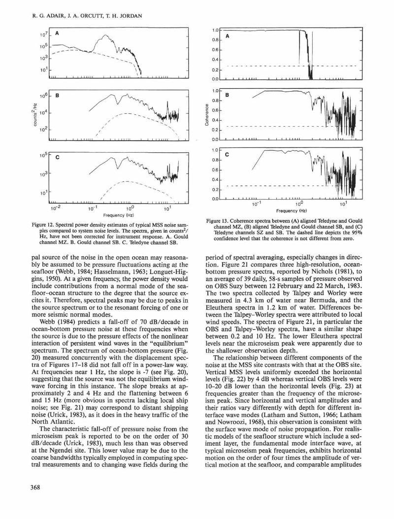
Figure 12 compares power spectral density estimatesof simultaneous vertical-component Teledyne and Goulddata with instrument noise spectra. The data are notcorrected for instrument response. The peaks above 8Hz in the SB spectra (Fig. 12B, C) are ship-generated.Peaks in the SB Teledyne spectrum (Fig. 12C) which areabsent in the short-period Gould spectrum (Fig. 12B)are manifestations of Teledyne aliasing. However, bothGould and Teledyne spectra have comparable values nearthe Nyquist frequency, implying that the Gould SB digi-tal low-pass filter was not functioning properly.

363


Teledyne data, Tape 5, Event 1. 039:0829:28.080-039:0844:28.080

-30000 30 35 40

Time (in min. after the hr.)

Figure 8. Typical example of seven-channel data from the Teledyne system. Channel identifications and am-plitudes, in digital counts, along the left. The event number is arbitrary.

Also shown in Figure 12 are estimates of system noise(dashed lines), provided by H. B. Durham of SandiaLaboratories. The system noise is not significant overthe entire short-period passband for either Teledyne orGould data. The white spectrum of quantizing noise forthe Teledyne data, from the uniformly distributed round-off errors of digital representation (see, e.g., Bendatand Piersol, 1971, pp. 231-232), has a level near 10~2

countsVHz, well below the Teledyne signal level. Esti-mates of the Gould digitizing noise level are not avail-able. Differences at frequencies greater than 4 Hz areprobably due to the combined effects of aliasing and ac-tual signal differences over the 175.5-cm sensor separa-tion. The MZ spectra (Fig. 12A) are similarly untaintedby system and sampling noise, and, furthermore, havesufficient frequency response roll-off at the high end toavoid aliasing.

Spectral coherences further delineate frequencies usa-ble for earth noise estimates. Mid-period coherences (Fig.13A) typically exceed 0.95 below the Gould low-pass fil-ter knee at 1.5 Hz except at 1 Hz, where it drops sharplyover a very narrow band of frequencies. The sharp dropis due to energy present in the Gould data but not theTeledyne, and may be related to the Gould digitizingscheme. Gould and Teledyne SB coherence (Fig. 13B)exceeds 0.8 between approximately 0.2 and 4.0 Hz. Thecoherence at higher frequencies declines amidst peakscaused by ship-generated signals. The sharp drops at ap-proximately 2 and 4 Hz are similar to that at 1 Hz in themidperiod coherence. The frequencies bounding the short-period band of high coherence varied a great deal dur-ing the MSS deployment, but generally were those shownin Figure 13B. Coherence estimates between SB and SZTeledyne data (Fig. 13C) were similar. In Figure 13, the

364


Gould data, Tape 5, Event 6. 039:0835:48.000—039:0850:48.000

1500

sz

-1500

40 r

SB

-4024 r

SX

_ -24C"o 1200

£ SY

-150

•\ h

H 1 1 1 h

H h H h

E -1200

30 r

MZ

-3020 r

MX

H h H 1 1 h

H h H 1 1 1

-20 L

150

MY

^ h H h H 1 \

i i i i

40 45Time (in min. after the hr.)

50

Figure 9. Typical example of seven-channel data from the Gould system during the first phase of MSS op-erations. Channel identifications and amplitudes, in digital counts (× I05) along the left. The eventnumber is arbitrary.

level below which the coherences do not significantly dif-fer (at the 95% confidence interval) from zero is shownwith dashed lines.

Figure 14 plots typical 4-channel OBS data collectedfrom a capsule employed to record refraction signals. Inthis figure, ship-generated noise dominates high frequencyfeatures on all channels. Since the OBSs have no redun-dant sensors, frequencies dominated by system and in-strument noise cannot be estimated from channel coher-ence.

The OBS dynamic range and resolution are modestcompared to those of the MSS systems, and, consequent-ly, limitations imposed by the sampling noise are moresevere in data recorded by the OBSs. As previously noted,two OBS instrument responses were employed during theNgendei Experiment. Since the refraction response ismore sensitive than the teleseismic response at high fre-quencies (see Fig. IB), the latter will be more limited at

lower frequencies. This is evident in Figure 15, whichcompares ambient and sampling noise estimates obtainedwith the two responses. The noise samples were not si-multaneous. Although most of the data composing theteleseismic-filter spectrum (solid upper curve) were re-corded after ship departure, its spectral levels exceed shipnoise levels measured with a refraction filter (dashedlower curve) at most frequencies. In the teleseismic spec-trum, sampling noise clearly dominates at frequenciesgreater than 15 Hz, and is probably significant in therange 7-18 Hz.

Ship-generated noise was estimated on a case-by-casebasis because it depended on which ship was proximalto an instrument and ship speed and activity. However,in general ship noise spectra were characterized by sharplydistinct peaks superimposed on a broadband level. Thefrequencies of most of the peaks were multiples of somefundamental, implying that the peaks were due to cavi-

365


"S 0.4 -

0.0 -

-200 -100 100 200

Lag (samples)

Figure 10. Cross-correlations of various channels of the Teledyne andGould systems. A positive lag corresponds to the second-namedchannel in the figure label being late with respect to the first namedchannel. A. Cross-correlation between Gould and Teledyne chan-nels MZ. B. Cross-correlation between Gould and Teledyne chan-nels SB. C. Cross-correlation of Teledyne's primary and backupSP vertical-component channels.

tation by ship propellers (e.g., Urick, 1983). Challengergenerated peaks at multiples of 10 Hz while maintainingstation. Two other peaks at approximately 6.5 and 7.5Hz were generated while it was under way. Peaks due toMelville were at multiples of 6 and 9 Hz.

Figure 16A compares vertical-component power den-sity spectra, corrected for gain but not instrument re-sponse, of OBS Phred data recorded before (solid curve)and after (dashed curve) both ships departed. The cap-sule, located 1.6 km west of the borehole, employed theteleseismic response. The measurement prior to ship de-parture was made at 0000Z, 12 Feb 1983, with both Chal-lenger and Melville hove to within 2 km of the OBS. Inthis instance, ship-generated noise clearly dominates thespectrum at all frequencies above approximately 4.5 Hz.After ship departure, least-count noise dominated above7 Hz, although the lowest frequency at which it domi-nated varied by ± 1 Hz because its level depends on OBSgain.

Some ambiguity exists concerning ship noise in theMSS data. Because the ocean-bottom recording systemfailed two days after its deployment, when Challengerwas 13 km away drilling Hole 596 and Melville was enroute to Tahiti, MSS noise measurements in the absenceof ships are not available. However, Challenger was brief-ly silent ca. 0510Z, 13 February, while monitoring anocean-bottom navigational transponder, thus providinga sample of low ship noise for the MSS. The MSS spec-trum of this time period is compared in Figure 16B with

that of data observed a short time later when Challengerbegan using the thrusters of its dynamic positioning sys-tem. Also shown in Figure 16B is an estimate of short-period system noise which has been scaled to fit the"quiet" spectrum. The good fit suggests that above 7Hz system noise dominates the spectrum.

The abrupt change of slope in the spectra of Figure16 is diagnostic of ship noise. On this basis, it is appar-ent from these and other spectra that ship noise may beimportant at frequencies as low as 3 Hz in both the OBSand MSS data.

The lowest valid frequency of OBS microseismic mea-surements is taken to be 0.1 Hz. At lower frequencies,least-count and system noise dominate. The latter sourceof noise was inferred from the lack of estimate stabilitywith regard to the number of spectra averaged in thepower density estimates.

Thus, in summary, reliable spectral estimates of am-bient seismic noise are available from MSS mid-perioddata between 0.2 and 1.5 Hz; from MSS short-perioddata between 0.2 and 7 Hz; and from OBS data between0.1 and 7 Hz. These bands are subject to the variabilityjust described that arises from the proximity of the ship,and OBS gain range and instrument response. At fre-quencies greater than 7 Hz, sampling noise dominatesOBS teleseismic data, so that lower bounds on ocean-bottom microseismic noise levels must be established us-ing data recorded with the refraction response.

RESULTS AND DISCUSSIONThe primary objectives of the noise analysis are the

comparison of noise levels recorded by the OBS and MSSsensors, and the investigation of noise generation andpropagation in the deep sea. Given the hypothesis thathigh-frequency (0.14-10 Hz) microseismic noise is com-posed principally of interface waves trapped near the sea-floor/ocean-bottom boundary, substantially lower noiselevels are anticipated at the MSS. This hypothesis is sup-ported by results from the Leg 78B MSS deployment(Adair et al., 1984).

Figures 17 and 18 show typical spectral estimates, cor-rected for instrument response, of simultaneous MSS andOBS observations in units of nmVHz. The data werecollected over a 70 min. period commencing 0840Z, 8February 1983. The estimates are averages of 10 individ-ual spectra. Each OBS spectrum was computed from13.02 s of data, whereas each MSS spectrum is a com-posite of mid-period and short-period spectra computedfrom, respectively, 128 and 12.8 s of Gould system data.The midperiod spectrum is shown at frequencies lessthan 1.4 Hz to achieve high-frequency resolution with aminimum of computation. The Gould spectral ampli-tudes have been adjusted by 3 dB to compensate for thedigital amplitude mismatch described above.

While the data of Figures 17 and 18 were collected,the OBS (Suzy) was 0.6 km north of the MSS site, Chal-lenger maintained station approximately 1.5 km north-west of the borehole, and Melville was completing Re-fraction Line 5 more than 170 km northwest of theborehole. Ship noise for all these spectra dominated atfrequencies greater than 4.5 Hz.

366


Frequency (Hz)

A, C:DMZ;OMX;ΔMYB, D: DSZ;OSX;ΔSY;OSB

10u

Frequency (Hz)

Figure 11. MSS sensor calibrations recorded by the Teledyne system during the first phase of the Ngendei Experiment for (A)midperiod and (B) short-period channels, and during the last phase for (C) midperiod and (D) short-period channels.

Differences between two spectra are significant at the95% confidence level if they exceed 5.5 dB (-2.3 and+ 3.2 dB). This assumes that the spectra are derived fromidentically distributed normal processes, so that eachestimate is x2-distributed with 2w degrees of freedom,where n = \0, the number of spectra averaged (Bendatand Piersol, 1971). For comparison, the 90% confidenceinterval is 4.7 dB.

The spectra have the usual overall appearance of earthnoise in this frequency band. They fall off rapidly to-ward higher frequencies from the microseism peak, whichtypically lies between 0.1 and 0.3 Hz. The ubiquitousmicroseism peak is generated by the nonlinear interac-tion of ocean surface waves having the same frequencybut traveling in opposite directions (Longuet-Higgins,1950). This interaction produces ocean-bottom pressurefluctuations that oscillate at twice the frequency of thegenerative surface waves. Although no wave spectrumdata are available for the Ngendei Experiment, a quali-tative description may be obtained from the deck andweather logs of Challenger. Swell periods of 6, 7, 9, 10,and 12 s were reported during the 4 hr. which precededand followed the noise observations of Figures 17-18.This corresponds to a double-frequency range of 0.17-

0.33 Hz, which is roughly the band of the observed mi-croseism peak.

At the microseism peak (approximately 0.2 Hz), lev-els at the seafloor and in the borehole on all compo-nents were within 5 dB of each other. In the band 0.6-4.5 Hz, vertical OBS levels exceeded those on the MSSby 10-15 dB (Fig. 17), and horizontal OBS levels exceed-ed the MSS levels by 25-30 dB (Fig. 18). This contrastswith results from Leg 78B (Fig. 19), in which vertical-component ocean-bottom levels observed 2 km from theMSS site exceeded borehole levels by 10 dB at the mi-croseism peak. Whereas the distances between the OBSand MSS were comparable for these two MSS deploy-ments, the sensor was much more deeply buried (519 m,with basement rock overlain by 93 m of sediment) onLeg 78B, suggesting that the depth of the Leg 91 sensorwas insufficient to achieve a significant reduction of noiselevels at the microseism peak. It was, however, appar-ently adequate at higher frequencies.

The irregular fall-off of the microseismic noise in Fig-ures 17-18, at 60-80 dB/decade, is punctuated by sev-eral peaks and slope breaks. These spectral characteris-tics are due to the combined influences of the sourcespectrum and the seafloor elastic structure. The princi-

367


1 0 6

1 0 4

1 0 2

- B

-

-

-—--NJ-

A• i lk J -

X,\ -

\

1Ob

10 3

101

c

-

-1

/ ^

1 1 i n i i i i 1 1 i n i i i i 11MI i i

10-210" 10u

Frequency (Hz)10'

Figure 12. Spectral power density estimates of typical MSS noise sam-ples compared to system noise levels. The spectra, given in counts2/Hz, have not been corrected for instrument response. A. Gouldchannel MZ. B. Gould channel SB. C. Teledyne channel SB.

pal source of the noise in the open ocean may reasona-bly be assumed to be pressure fluctuations acting at theseafloor (Webb, 1984; Hasselmann, 1963; Longuet-Hig-gins, 1950). At a given frequency, the power density wouldinclude contributions from a normal mode of the sea-floor-ocean structure to the degree that the source ex-cites it. Therefore, spectral peaks may be due to peaks inthe source spectrum or to the resonant forcing of one ormore seismic normal modes.

Webb (1984) predicts a fall-off of 70 dB/decade inocean-bottom pressure noise at these frequencies whenthe source is due to the pressure effects of the nonlinearinteraction of persistent wind waves in the "equilibrium"spectrum. The spectrum of ocean-bottom pressure (Fig.20) measured concurrently with the displacement spec-tra of Figures 17-18 did not fall off in a power-law way.At frequencies near 1 Hz, the slope is -7 (see Fig. 20),suggesting that the source was not the equilibrium wind-wave forcing in this instance. The slope breaks at ap-proximately 2 and 4 Hz and the flattening between 6and 15 Hz (more obvious in spectra lacking local shipnoise; see Fig. 21) may correspond to distant shippingnoise (Urick, 1983), as it does in the heavy traffic of theNorth Atlantic.

The characteristic fall-off of pressure noise from themicroseism peak is reported to be on the order of 30dB/decade (Urick, 1983), much less than was observedat the Ngendei site. This lower value may be due to thecoarse bandwidths typically employed in computing spec-tral measurements and to changing wave fields during the

1.0

0.8

0.6

0.4

0.2

0.0

A

•::v.:::";v:.::"i

101"Frequency (Hz)

10'

Figure 13. Coherence spectra between (A) aligned Teledyne and Gouldchannel MZ, (B) aligned Teledyne and Gould channel SB, and (C)Teledyne channels SZ and SB. The dashed line depicts the 95%confidence level that the coherence is not different from zero.

period of spectral averaging, especially changes in direc-tion. Figure 21 compares three high-resolution, ocean-bottom pressure spectra, reported by Nichols (1981), toan average of 39 daily, 58-s samples of pressure observedon OBS Suzy between 12 February and 22 March, 1983.The two spectra collected by Talpey and Worley weremeasured in 4.3 km of water near Bermuda, and theEleuthera spectra in 1.2 km of water. Differences be-tween the Talpey-Worley spectra were attributed to localwind speeds. The spectra of Figure 21, in particular theOBS and Talpey-Worley spectra, have a similar shapebetween 0.2 and 10 Hz. The lower Eleuthera spectrallevels near the microseism peak were apparently due tothe shallower observation depth.

The relationship between different components of thenoise at the MSS site contrasts with that at the OBS site.Vertical MSS levels uniformly exceeded the horizontallevels (Fig. 22) by 4 dB whereas vertical OBS levels were10-20 dB lower than the horizontal levels (Fig. 23) atfrequencies greater than the frequency of the microse-ism peak. Since horizontal and vertical amplitudes andtheir ratios vary differently with depth for different in-terface wave modes (Latham and Sutton, 1966; Lathamand Nowroozi, 1968), this observation is consistent withthe surface wave mode of noise propagation. For realis-tic models of the seafloor structure which include a sed-iment layer, the fundamental mode interface wave, attypical microseism peak frequencies, exhibits horizontalmotion on the order of four times the amplitude of ver-tical motion at the seafloor, and comparable amplitudes

368

Event 150

Channel VERTMAX: 3.60E+00Y-TIC 0.5E+ 00<Y>:-2.52E-02No filter

OBS Suzy 1342:00.131 3 FEB 83


DECI: 1

Channel HORIMAX: 9.04E+00Y-TIC:0.2E+01<Y>:-3.38E-02No filter

Channel H0R2MAX: 6.22E+00Y-TIC:0.1E+01<T>:-2.62E-02No filter

Channel HYDRMAX: 9.43E-01Y-TIC:0.2E+00<Y>: 2.57E-02No filter

10 12

Time (s)

Figure 14. Example of 4-channel OBS data recorded with the refraction instrument response. Data are from OBS Suzy.Amplitudes are given in gain-corrected counts and each channePs plot has been individually scaled. Channels are,from top to bottom, vertical, two horizontals, and hydrophone.

for the two components within competent basementrock (Latham and Sutton, 1966). Future analysis of theNgendei noise data will model these observations to fur-ther constrain the propagation mode of the noise.

The microseism peak and a 0.4 Hz-wide band cen-tered at 1 Hz display high coherence and a cross-phase ofapproximately 180° (Fig. 24A and B) between the pres-sure and vertical displacement. It may be shown that ata fluid-solid interface, kinematic boundary conditionsrequire a 180° phase shift for both normally incidentplane waves reverberating in the water column (Schneiderand Backus, 1964) and for trapped modes of the ocean-seafloor elastic system (Bradner, 1962; Schneider et al.,1964; Latham and Sutton, 1966). For plane waves, thepressure-seismic velocity ratio is constant with frequencyand equals the product of density p and acoustic speeda in the water, 1.5 × I06 in MKS units, whereas for trappedmodes it may vary with frequency and exceed pa (Brad-ner, 1962; Latham and Nowroozi, 1968). Figure 24Cplots the ratio between the pressure and vertical-compo-

nent velocity power density spectra, normalized by (pa)2.Over the two bands of high coherence, this ratio is on theorder of 10, rather than one, suggesting that in this in-stance the bands represent trapped seismic modes. Thus,in this case, the practice of comparing seismic groundvelocities V(f) to a "plane-wave equivalent" pressure P(f)via the relation P=pcV is quite incorrect.

Coherences between OBS capsule pairs were computedto investigate noise field propagation. Figure 25 showsthe coherence and cross-phase between the vertical andhydrophone channels of OBSs Suzy and Lynn, separatedby 0.6 km, for the same time interval as above. Again,energy at the microseism peak is highly coherent. Thecross-phase at these frequencies is not significantly dif-ferent from zero, implying either simultaneous arrivalof microseism energy at the two capsules or a wave-length much larger than the capsule separation. Lathamet al. (1967) calculate the dispersion curves for trappedmodes in an ocean-bottom structure similar to that ofthe Ngendei site. At these frequencies the fundamental

369


1 0 1 2

10 c

I ,0-

10 -4

TeleseismicRefraction

10-1 10u 10'Frequency (Hz)

Figure 15. Comparison of noise spectrum obtained with the teleseis-mic (solid upper curve) and refraction (dashed upper curve) OBSresponses. The corresponding instrumentally corrected samplingnoise spectra (lower curves) are also shown.

10" 10'Frequency (Hz)

Figure 16. Illustration of ship noise in the (A) OBS and (B) MSS data.Solid spectra were observed when ships were nearby and operation-al, and the dashed spectra when ships were completely absent(OBS) or still nearby (MSS). MSS data are not available at anytime when ships were completely absent.

mode has a phase velocity Cp of 1.0-1.5 km/s, corre-sponding to a wavelength λ = Cp/f on the order of 5 km.The capsule separation, roughly λ/10, is too large to ac-count for the observed small cross-phases; this rules outthe oblique arrival of the microseism energy from a dis-tant source. It therefore appears that the microseismsource location in this instance is either local or along aline that is approximately normal to a line defined by

TTT 1 I I I I TT I 1 1 1 I T i l l T

10 10

Frequency (Hz)

Figure 17. Simultaneous vertical-component displacement power den-sities at the ocean bottom (dashed line) and in the borehole (solidline).

10v

Frequency (Hz)

10'

Figure 18. Simultaneous horizontal-component displacement powerdensities at the ocean bottom (dashed line) and in the borehole(solid line).

the OBSs. Coherences between OBSs Juan and Lynn,separated by 0.7 km, exhibit similar coherences and cross-phases near the microseism peak.

The vertical-component spectra of Figure 17 are com-pared in Figure 26 with extrema of similar measurementsfrom Scripps Institution of Oceanography (SIO) OBSs.Above ~ 1.5 Hz, the Leg 91 measurements are compara-ble to the lower extreme and fall off at a similar rate.This is despite the fact that the observation sites andconditions were quite disparate. The extrema are notwell defined at lower frequencies because of the shortdata sample lengths from which the spectra were ob-tained.

Figure 27 compares the Figure 17 spectra to unusu-ally low noise observations on land. The Lajitas spec-

370


10° -

i 10-

Y 10'

α> . 1E 1 0 π

α>

Q Λ

10 4

I I \ I M i l l I I I I I I I I I

I I I I I I I 1 1 1 1 1 1 1 11 1

10" 10 u

Frequency (Hz)

10'

Figure 19. A comparison of vertical-component ocean-bottom andborehole noise levels observed during DSDP Leg 78B (dashedcurves) and during the Ngendei Experiment, Leg 91 (solid curves).

1 0 v

g 10

CO

10-5

i i i 1 1 m i i i i i

10

Frequency (Hz)

Figure 20. Ocean-bottom pressure measurements concurrent with thedisplacement spectra of Figure 17.

trum (Herrin, 1982) is representative of the quietest knownsite, which is near the Big Bend of the Rio Grande Riv-er. At frequencies less than 2 Hz, Lajitas noise levels dif-fer little from those measured at a quiet site in a mineshaft near Queen Creek, Arizona (Fix, 1972; Melton,1976), so their composite delineates the lowest knownnoise levels at these frequencies. The MSS levels exceedthis composite by 20-35 dB below 2 Hz, but converge towithin 10 dB at higher frequencies. The OBS levels simi-larly exceed the composite by 35-45 dB below 2 Hz, andconverge to within 30 dB above 2 Hz. The 10 Hz peak inthe Lajitas spectrum is not related to that in the Ngendeispectra, which is ship-generated.

CONCLUSIONS

Comparable noise levels were observed at the microse-ism peak on all components at both the ocean bottom andin the borehole. However, at higher frequencies (0.3-4.5Hz), the borehole noise levels were substantially lowerthan the ocean-bottom levels for both vertical and hori-zontal components. If microseism peak noise is a trappedwave phenomenon, then the observation that the noiselevels were comparable in the OBS and MSS at the mi-croseism peak suggests that the borehole sensor was notsufficiently deep in the basaltic basement to diminishnoise levels over the entire band of frequencies.

The analysis has yielded several constraints on bothsource character and noise propagation. The microse-ism peak displayed high coherence and a cross-phaseconsistent with simultaneous arrival over a distance ofat least 0.7 km. This suggests a local source for noise inthe microseism peak range. The rate of fall-off of theOBS and MSS spectra from the microseism peak andthe variety of peaks in the fall-off indicate both regionaland local sources for noise in this frequency range. Thepeaks are probably due both to source spectrum shapeand to resonant forcing of seismic modes trapped nearthe seafloor-ocean-bottom interface. The observed ver-tical- and horizontal-component noise levels in the bore-hole and at the ocean bottom constrain the mode ofnoise propagation. In the MSS vertical component, noisewas insignificantly (4 dB) higher than the noise levelsmeasured in the horizontal components, whereas therewas a 10-20 dB difference in the OBS horizontal andvertical component noise levels. Since changes with depthin horizontal amplitude and the ratio of horizontal tovertical amplitudes are different for different types ofinterface waves, detailed investigation of these differenceswould constrain the mode of noise propagation.

Spectral slopes of the pressure noise at frequenciesless than approximately 2 Hz were not consistent in theinstances considered here with those expected from equi-librium wind-wave generation. The flattening of the pres-sure spectrum seen at frequencies greater than 2 Hz isprobably due to distant shipping noise.

The borehole noise levels observed during the Ngen-dei Experiment are comparable to average continentalsites, and approach exceptionally quiet land levels onlyat frequencies above 10 Hz. Deeper burial may have someeffect on the noise levels, reducing levels in the microse-ism peak somewhat closer to levels in quiet land sites.

Modeling of the phase spectrum, relative amplitudesand coherences between different sites and components,and spectral shape should yield a better more sophisti-cated characterization of the noise and source fields.These phenomena will be the subject of further researchusing the Ngendei noise data.

ACKNOWLEDGMENTS

The authors thank Chip Cox for his useful review. This researchwas supported by DARPA contracts F49620-79-C-0019 and AFOSR-84-0043.

REFERENCES

Adair, R. G., Orcutt, J. A., and Jordan, T. H., 1984. Analysis of am-bient seismic noise recorded by downhole and ocean-bottom seis-

371


mometers on Deep Sea Drilling Project Leg 78B. In Hyndman, R.D., Salisbury, M. H., et al., Init. Repts. DSDP, 78B: Washington(U.S. Govt. Printing Office), 767-781.

Bendat, J. S., and Piersol, G. G., 1971. Random Data: Analysis andMeasurement Procedures: New York (John Wiley).

Bradner, H., 1962. Pressure variations accompanying a plane wavepropagated along the ocean bottom. J. Geophys. Res., 67:3631-3633.

Bradner, H., and Dodds, J. G., 1964. Comparative seismic noise onthe ocean bottom and on land. J. Geophys Res., 69:4339-4348.

Creager, K. C , and Dorman, L. M., 1982. Locations of instrumentson the seafloor by joint adjustment of instrument and ship posi-tions. J. Geophys. Res., 87:8379-8388.

Duennebier, F. K., and Blackinton, G., 1983. The ocean subbottomseismometer. In Geyer, R. (Ed.), Geophysical Exploration at Sea:Boca Raton (CRC Press), 317-332.

Fix, J. E., 1972. Ambient earth motion in the period range from 0.1 to2560 sec. Bull. Seism. Soc. Am., 62:1753-1760.

Hasselmann, K., 1963. A statistical analysis of the generation of mi-croseisms. Rev. Geophys., 1:177-210.

Herrin, E., 1982. The resolution of seismic instruments used in treatyverification research. Bull. Seism. Soc. Am., 72:S61-S67.

Hyndman, R. D., Salisbury, M. H., et al., 1984. Init. Repts. DSDP,78B: Washington (U.S. Govt. Printing Office).

Jenkins, G. M., and Watts, D. G., 1968. Spectral Analysis and its Ap-plications: San Francisco (Holden-Day).

Latham, G. V., Anderson, R. S., and Ewing, M., 1967. Pressure vari-ations produced at the ocean bottom by hurricanes. J. Geophys.Res., 72:5693-5704.

Latham, G. V., and Nowroozi, A. A., 1968. Waves, weather, and oceanbottom microseisms. /. Geophys. Res., 73:3945-3956.

Latham, G. V., and Sutton, G. H., 1966. Seismic measurements onthe ocean floor, 1. Bermuda area. J. Geophys. Res., 71:2545-2572.

Longuet-Higgins, M. S., 1950. A theory of the origin of microseisms.Phil. Trans. R. Soc. London, A, 243:1-35.

Melton, B. S., 1976. The sensitivity and dynamic range of inertial seis-mographs. Rev. Geophys. Space Phys., 14:93-116.

Moore, R. D., Dorman, L., Huang, C.-Y., and Berliner, D. L., 1981.An ocean bottom, microprocessor based seismometer. Mar. Geo-phys. Res., 4:451-477.

Nichols, R. H., 1981. Infrasonic ambient ocean noise measurements:Eleuthera. /. Acoust. Soc. Am., 69:974-981.

Otnes, R. K., and Enochson, L., 1982. Digital Time Series Analysis:New York (John Wiley).

Prentiss, D. D., and Ewing, J. I., 1963. The seismic motion of thedeep ocean floor. Bull. Seism. Soc. Am., 53:765-781.

Schneider, W. A., and Backus, M. M., 1964. Ocean-bottom seismicmeasurements off the California coast. J. Geophys. Res., 69:IBS-IMS.

Schneider, W. A., Farrell, P. J., and Brannian, R. E., 1964. Collectionand analysis of Pacific ocean-bottom seismic data. Geophysics, 29:745-771.

Singleton, R. C , 1969. An algorithm for computing the mixed radixfast Fourier transform. IEEE Trans. Audio Electroacoust., AU-17:93-103.

Spudich, P., and Orcutt, J., 1980. Petrology and porosity of an ocean-ic crustal site: Results from wave form modeling of seismic refrac-tion data. J. Geophys. Res., 85:1409-1433.

Stephen, R. A., Johnson, S., and Lewis, B., 1983. The oblique seis-mic experiment on Deep Sea Drilling Project Leg 65. In Lewis, B.T. R., Robinson, P., et al., Init. Repts. DSDP, 65: Washington(U.S. Govt. Printing Office), 319-328.

Stephen, R. A., Louden, K. E., and Matthews, D. H., 1980. Theoblique seismic experiment on Deep Sea Drilling Project Leg 52.In Donnelly, T., Francheteau, J., Bryan, W., Robinson, P., Flower,M., Salisbury, M., et al., Init. Repts. DSDP, 51, 52, 53, Pt. 1:Washington (U.S. Govt. Printing Office), 675-704.

Sutton, G. H., Duennebier, F. K., and Iwatake, B., 1981. Coupling ofocean bottom seismometers to soft bottom. Mar. Geophys. Res.,5:35-51.

Urick, R. J., 1974. Sea-bed motion as a source of the ambient noisebackground of the sea. /. Acoust. Soc. Am., 56:1010-1011.

, 1983. Principles of Underwater Sound (3rd ed.): New York(McGraw-Hill).

Webb, S. C , 1984. Observations of seafloor pressure and electric fieldfluctuations [Ph.D. dissert.]. University of California, San Diego.

Welch, P. D., 1967. The use of Fast Fourier Transform for the estima-tion of power spectra: A method based on time averaging overshort, modified periodograms. IEEE Trans. Audio Electro-acoust.,AU-15:70-73.

Date of Initial Receipt: 14 February 1985Date of Acceptance: 28 January 1986

372


10'

£ 102

to 1 0

10 -4

I I I I I I i i i i M in i i \ i Π^TTI r i i i i i i i i

D Talpey-Worley (1 7.5 kt.)O Talpey-Worley (1 2.4 kt.)Δ Eleuthera— SW Pacific

I i i i i i i i i L i i i i M M i i i i i i i i i i i i i i i i I

10" 1 0 u

Frequency (Hz)

1 0 '

Figure 21. Ocean-bottom pressure measurements observed on OBS Suzy at 5.6 km water depth, during theperiod 12 February-22 March 1983, compared with high-resolution measurements reported by Nichols(1981). See text for explanation of key. Given for the Talpey-Worley spectra are the average wind speedsduring data collection.

Frequency (Hz)

1 0 '

Figure 22. Simultaneous vertical (solid) and horizontal (dashed) powerdensities in the borehole.

~ 10°N

J ,0»

^ 10'

1 10"1

E

S io- 4

I I I I I T I 1 1 1

10 -1I I I I I I

1 0 u

Frequency (Hz)10'

Figure 23. Simultaneous vertical (solid) and horizontal (dashed) powerdensities at the ocean bottom.

373


1.0

0.8

0.6

0.4

0.2

0.0

A

\

V\ 1\J

1 1 1 _

" \ / ^ 1 \~

i i i -

1.0

^ 0.5CDto

CO

Q. 0.0toCO

§-0.5

-1.0

— I >

B

V

- I I

1 1 1 -

A A

i i i -

1.0Frequency (Hz)

Figure 24. (A) Coherence and (B) cross-phase between OBS Suzychannels Z (vertical) and P (hydrophone). The cross-phase, plottedin multiples of π, has been corrected for instrument responsephase. C. The ratio between OBS Suzy pressure and verticalground-velocity power densities, normalized by the product ofdensity and acoustic speed in the water.

1.0

0.8

Coh

eren

ceo

o

0.2

0.0

_ I 1

- / \

_ \

\ A /

i i _

-

-

\ * * \ / \ ~

1 1 -

1.0

0.5

0.0

-1.0

- i 1

B

-

i i —

i

0.0 0.5 1.0Frequency (Hz)

1.5 2.0

Figure 25. (A) Coherence and (B) cross-phase between the verticalchannels of OBSs Suzy and Lynn, as for Figure 24.

10° -

Y 10Φ

1c , n • 1

2 _

10"' -

.12 10Q

-4

I M i l

—-~-

\ /

I I | I I

OBS Suzy

V

i I I I I

i i 11 i

MSS V N

i i i i i i 11 i

-

^ - ' \ 1

10" 1 0 '

Frequency (Hz)

Figure 26. Comparison of vertical-component noise of Figure 17 withextrema (dashed lines) observed on Scripps Institution of Ocean-ography OBSs during their 12-yr. program.

374


10c

10

° 10'α>

Q 1 0 " 4

i i i T T i r i i i i i i 111

J i i i i i 111

10 10'

Frequency (Hz)

Figure 27. Comparison of vertical component noise observations fromthe Ngendei Experiment with extremely low level observations atland sites. The composite of the Queen Creek and Lajitas spectramay be taken as the lowest known microseism levels at these fre-quencies.

375

during the ngendei experiment1 · the mss sensors are four teledyne model s-750 seis-mometers...

Documents