draft of mathl. comput. modelling 15 77-98. application of

Draft of L. Ingber, M.F. Wehner, G.M. Jabbour, and T.M. Barnhill, “Application of statistical mechanicsmethodology to term-structure bond-pricing models,”Mathl. Comput. Modelling15 (11), 1991, pp.77-98.

Application of Statistical Mechanics Methodologyto Term-Structure Bond-Pricing Models

Lester IngberScience Transfer Corporation

P.O. Box 857McLean, VA 22101

Michael F. WehnerB Division

Lawrence Livermore LaboratoryLivermore, CA 94550

George M. Jabbour and Theodore M. BarnhillDepartment of Business Administration

The George Washington UniversityWashington, DC 20052

Statistical Mechanics Methodology - 2 - Ingber, Wehner, Jabbour, Barnhill

ABSTRACTRecent work in statistical mechanics has developed new analytical and numerical techniques to solvecoupled stochastic equations. This paper applies the very fast simulated re-annealing and path-integralmethodologies to the estimation of the Brennan and Schwartz two-factor term structure model. It isshown that these methodologies can be utilized to estimate more complicatedn-factor nonlinear models.

1. CURRENT MODELS OF TERM STRUCTUREThe modern theory of term structure of interest rates is based on equilibrium and arbitrage models inwhich bond prices are determined in terms of a few state variables. The one-factor models of Cox,Ingersoll and Ross (CIR) [1-4], and the two-factor models of Brennan and Schwartz (BS) [5-9] have beeninstrumental in the development of the valuation of interest dependent securities. The assumptions ofthese models include:

• Bond prices are functions of a number of state variables, one to several, that follow Markovprocesses.

• Inv estors are rational and prefer more wealth to less wealth.

• Inv estors have homogeneous expectations.

• No one investor is big enough to affect market prices.

• Taxes and transaction costs are not modeled.

• Information is costless and available to all.

• Assets are traded continuously at equilibrium prices.

However, it should be noted that the ‘‘efficient market’’ hypothesis is not quite universallyaccepted [10-12].

For one-factor models, the state variable is assumed to be the short-term interest rate which isassumed to follow a diffusion process or a continuous Markov process defined as follows:

dr = a(r , t)dt + b(r , t)dz ,

r = short-term rate,t = calendar time,a(r , t) = expected instantaneous change in the short-term rate,b(r , t) = instantaneous volatility of the process,dz is a Wiener process.

(1)

Bond prices are assumed to be a function of time and a proxy variable, the short-term rate.

Vasicek [4] assumes that

dr = K (θ − r )dr + σ rdz . (2)

CIR assume

dr = K (θ − r )dr + σ r 1/2dz . (3)

In both models, short-term rates are assumed to follow a mean-reverting process; in other words, theshort-term rates have a mean ofθ , K being the speed of adjustment.σ r and σ r 1/2 are the standarddeviations of the random component of the process for Vasicek and CIR models, respectively.

BS [5] extended the one factor model. They dev eloped an arbitrage model of equilibrium interestrates based on the assumptions that the entire term structure at any point in time can be expressed as afunction of two factors, being the short- and long-term rates of default free instruments. These interestrates are further assumed to follow a joint Wiener stochastic process. This process is of the form:

dr = β1(r , l , t)dt + η1(r , l , t)dz1 ,


dl = β2(r , l , t)dt + η2(r , l , t)dz2 , (4)

wherer and l are the short- and long-term rates, respectively.β1 and β2 are the expected instantaneousrates of change in the short-term and long-term rates respectively.η1 and η2 are the instantaneousstandard deviations of the processes.dz1 anddz2 are Wiener processes, with expected values of zero andvariance ofdt with correlation coefficientρ. That is,

E[dz1] = E[dz2] = 0 ,

E[dz21] = E[dz2

2] = dt , E[dz1dz2] = ρdt , (5)

whereE[. ] ≡ < . > is the expectation with respect to the joint Wiener process.

For estimation purposes, BS simplified and reduced this system to

dr = ((a1 + b1(l − r )))dt + rσ1dz1 ,

dl = l (a2 + b2r + c2l )dt + lσ2dz2 , (6)

where{ a1, b1, a2, b2, c2} are parameters to be estimated.

These equations imply that the short-term rate converges towards a long-term rate (b1 > 0). Aresult found in part of the BS study isa1 < 0, i.e., the short-term rate could be negative. This is apotentially serious problem for this model.

The BS discrete-time representation is

r t+1 − r t

r t=

a1

r t+ b1(

l t

r t− 1) + e1t ,

l t+1 − l t

l t= a2 + b2r t + c2l t + e2t , (7)

wheree1t ande2t are normally-distributed bivariate random variables with standard deviations ofσ1 andσ2 respectively with a correlation coefficient ofρ. As discussed below, the above continuous model isonly well defined in the differential limit of these discrete equations.

These equations imply that the short-term rate converges towards the long-term rate (b1 > 0). Aresult found in part of the BS study is thata1 < 0. i.e., the short-term rate could be negative if not subjectto an additional external boundary condition. This is a potentially serious problem for this model. BSused the iterative Aitken procedure [13] to estimate the parameters of the model. They founda1 to benegative (the long-term rate has to be larger than 2% to avoid negative short-term rates). The correlationcoefficient ρ, and the coefficientsa1 and b1 were unstable. In addition, BS found a negative serialcorrelation in the error termse1t ande2t , which led them to believe that additional state variables shouldbe added to the model.

Using methods of stochastic calculus [5], BS further derived a partial differential equation for bondprices as the maturity date is approached.

∂∂τ

B = ((−r + f r ∂∂r

+ f l ∂∂l

+ grr ∂∂r 2

+ grl ∂∂r∂l

+ gll ∂∂l2

))B

= AB , (8)

where the coefficients{ f , g} depend onr and l , τ = T − t for t calendar time andT the time of maturity,andA can be considered as a differential operator onB.

It may help to appreciate the importance of the BS methodology by discretizing the above partialdifferential equation forB, in a ‘‘mean-value’’ limit. That is, at a given calendar timet indexed bys,noting that∂/∂τ = −∂/∂t, take

0 = f r ∂Bs

∂r= f l ∂Bs

∂l,


0 = grr ∂Bs

∂r 2= grl ∂Bs

∂r∂l= gll ∂Bs

∂l2,

Bs − Bs+1 = −r sBs . (9)

This yields the popular expectations-hypothesis spot-interest estimate of bond prices, working backwardsfrom maturity,

Bs = (1 + r s)−1Bs+1 . (10)

The important generalization afforded by BS is to include information aboutr and l and treat themas stochastic variables with drifts and diffusions. Then, this discretized treatment yields

Bs rl = (1 − As rlr ′ l ′)−1Bs+1 r ′ l ′ , (11)

where the operator inverse of the differential operatorA has been formally written, and its dependence onintermediate values ofr ′ andl ′ has been explicitly portrayed. Their discretized calculation of their partialdifferential equation, and our discretized calculation of the path-integral representation of this model,essentially are mathematical and numerical methods of calculating this evolution ofBs.

In this paper we present an alternative methodology of very fast simulated re-annealing(VFSR) [14] to compute the parameters of the BS model. It is also shown that the VFSR methodology iscapable of handling more complicatedn-factor nonlinear models.

The advantages of using the simulated annealing methodology are: (1) Global minima in parameterspace are relatively more certain than with regression fitting. (2) All parameters, including parameters inthe noise, are simultaneously and equally treated in the fits, i.e., different statistical methods are not beingused to estimate the deterministic parameters, then to go on to estimate noise parameters. (3) Boundaryconditions on the variables can be explicitly included in the fitting process, a process not included instandard regression fits. (4) We can efficiently extend our methodology to develop 3-state and highermodels, including higher order nonlinearities.

We also present an alternative method of calculating the evolution of bond prices. Our particularnon-Monte Carlo path-integral technique has proven to be extremely accurate and efficient for a variety ofnonlinear systems [15,16]. The method of path integration is more accurate and efficient for calculatingthe evolution ofB as a function of the stochastic variablesr and l . To mention a few advantages: (1) Avariable mesh is calculated in terms of the underlying nonlinearities. (2) Initial conditions and boundaryconditions typically are more easily implemented with integral, rather that with differential, equations,e.g., by using the method of images. (3) Integration is inherently a ‘‘smoothing’’ process, whereasdifferentiation is a ‘‘sharpening’’ process. This means that we can handle ‘‘stiff’’ and nonlinear problemswith more ease.

We also comment below on how our methodology can be applied to other future-price modelsunder development [17-19].

In Section 2, we give a brief theoretical description of mathematically equivalent representations ofmultivariate stochastic systems. These methods, just recently developed by mathematical physicists in thelast decade in the context of ‘‘statistical mechanics,’’ permit the introduction of even more recentlydeveloped numerical algorithms. They were proposed for financial systems in a previous paper [20].

In Section 3, we apply this formalism to specific computations of the BS model. Section 4 givesour numerical results. Section 5 presents our conclusions. Appendix A gives a derivation of thestochastic calculus used.

2. DEVELOPMENT OF MATHEMATICAL METHODOLOGY

2.1. BackgroundAggregation problems in nonlinear nonequilibrium systems typically are ‘‘solved’’

(accommodated) by having new entities/languages developed at these disparate scales in order toefficiently pass information back and forth [21,22]. This is quite different from the nature of quasi-


equilibrium quasi-linear systems, where thermodynamic or cybernetic approaches are possible. Theseapproaches typically fail for nonequilibrium nonlinear systems.

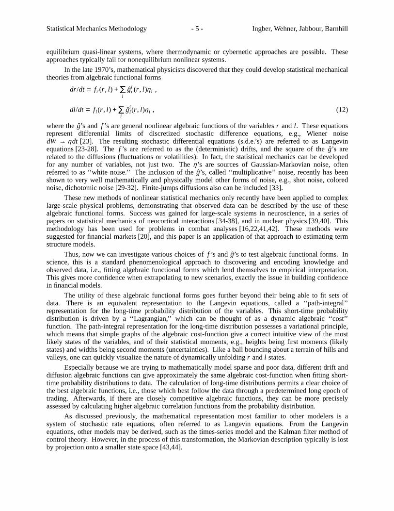
In the late 1970’s, mathematical physicists discovered that they could develop statistical mechanicaltheories from algebraic functional forms

dr/dt = fr (r , l ) +iΣ gi

r (r , l )η i ,

dl/dt = fl (r , l ) +iΣ gi

l (r , l )η i , (12)

where the ˆg’s and f ’s are general nonlinear algebraic functions of the variablesr and l . These equationsrepresent differential limits of discretized stochastic difference equations, e.g., Wiener noisedW → η dt [23]. The resulting stochastic differential equations (s.d.e.’s) are referred to as Langevinequations [23-28]. Thef ’s are referred to as the (deterministic) drifts, and the square of the ˆg’s arerelated to the diffusions (fluctuations or volatilities). In fact, the statistical mechanics can be developedfor any number of variables, not just two. Theη ’s are sources of Gaussian-Markovian noise, oftenreferred to as ‘‘white noise.’’ The inclusion of the ˆg’s, called ‘‘multiplicative’’ noise, recently has beenshown to very well mathematically and physically model other forms of noise, e.g., shot noise, colorednoise, dichotomic noise [29-32]. Finite-jumps diffusions also can be included [33].

These new methods of nonlinear statistical mechanics only recently have been applied to complexlarge-scale physical problems, demonstrating that observed data can be described by the use of thesealgebraic functional forms. Success was gained for large-scale systems in neuroscience, in a series ofpapers on statistical mechanics of neocortical interactions [34-38], and in nuclear physics [39,40]. Thismethodology has been used for problems in combat analyses [16,22,41,42]. These methods weresuggested for financial markets [20], and this paper is an application of that approach to estimating termstructure models.

Thus, now we can investigate various choices off ’s and g’s to test algebraic functional forms. Inscience, this is a standard phenomenological approach to discovering and encoding knowledge andobserved data, i.e., fitting algebraic functional forms which lend themselves to empirical interpretation.This gives more confidence when extrapolating to new scenarios, exactly the issue in building confidencein financial models.

The utility of these algebraic functional forms goes further beyond their being able to fit sets ofdata. There is an equivalent representation to the Langevin equations, called a ‘‘path-integral’’representation for the long-time probability distribution of the variables. This short-time probabilitydistribution is driven by a ‘‘Lagrangian,’’ which can be thought of as a dynamic algebraic ‘‘cost’’function. The path-integral representation for the long-time distribution possesses a variational principle,which means that simple graphs of the algebraic cost-function give a correct intuitive view of the mostlikely states of the variables, and of their statistical moments, e.g., heights being first moments (likelystates) and widths being second moments (uncertainties). Like a ball bouncing about a terrain of hills andvalleys, one can quickly visualize the nature of dynamically unfoldingr andl states.

Especially because we are trying to mathematically model sparse and poor data, different drift anddiffusion algebraic functions can give approximately the same algebraic cost-function when fitting short-time probability distributions to data. The calculation of long-time distributions permits a clear choice ofthe best algebraic functions, i.e., those which best follow the data through a predetermined long epoch oftrading. Afterwards, if there are closely competitive algebraic functions, they can be more preciselyassessed by calculating higher algebraic correlation functions from the probability distribution.

As discussed previously, the mathematical representation most familiar to other modelers is asystem of stochastic rate equations, often referred to as Langevin equations. From the Langevinequations, other models may be derived, such as the times-series model and the Kalman filter method ofcontrol theory. Howev er, in the process of this transformation, the Markovian description typically is lostby projection onto a smaller state space [43,44].


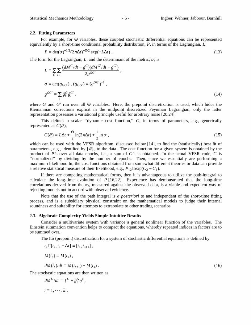
2.2. Fitting ParametersFor example, forΘ variables, these coupled stochastic differential equations can be represented

equivalently by a short-time conditional probability distribution,P, in terms of the Lagrangian,L:

P = det(σ )−1/2(2π∆t)−Θ/2 exp(−L∆t) . (13)

The form for the Lagrangian,L, and the determinant of the metric,σ , is

L =GΣ

G′Σ (dMG/dt − gG)(dMG′ /dt − gG′)

2gGG′ ,

σ = det(gGG′) , (gGG′) = (gGG′)−1 ,

gGG′ =iΣ gG

i gG′i , (14)

where G and G′ run over allΘ variables. Here, the prepoint discretization is used, which hides theRiemannian corrections explicit in the midpoint discretized Feynman Lagrangian; only the latterrepresentation possesses a variational principle useful for arbitrary noise [20,24].

This defines a scalar ‘‘dynamic cost function,’’C, in terms of parameters, e.g., genericallyrepresented asC(α ),

C(α ) = L∆t +Θ

2ln(2π∆t) +

1

2ln σ , (15)

which can be used with the VFSR algorithm, discussed below [14], to find the (statistically) best fit ofparameters , e.g., identified by{ α } , to the data. The cost function for a given system is obtained by theproduct of P’s over all data epochs, i.e., a sum ofC’s is obtained. In the actual VFSR code,C is‘‘normalized’’ by dividing by the number of epochs. Then, since we essentially are performing amaximum likelihood fit, the cost functions obtained from somewhat different theories or data can providea relative statistical measure of their likelihood, e.g.,P12∼ exp(C2 − C1).

If there are competing mathematical forms, then it is advantageous to utilize the path-integral tocalculate the long-time evolution ofP [16,22]. Experience has demonstrated that the long-timecorrelations derived from theory, measured against the observed data, is a viable and expedient way ofrejecting models not in accord with observed evidence.

Note that the use of the path integral isa posteriori to and independent of the short-time fittingprocess, and is a subsidiary physical constraint on the mathematical models to judge their internalsoundness and suitability for attempts to extrapolate to other trading scenarios.

2.3. Algebraic Complexity Yields Simple Intuitive ResultsConsider a multivariate system with variance a general nonlinear function of the variables. The

Einstein summation convention helps to compact the equations, whereby repeated indices in factors are tobe summed over.

The Ito(prepoint) discretization for a system of stochastic differential equations is defined by

ts∈ [ts, ts + ∆t] ≡ [ts, ts+1] ,

M(ts) = M(ts) ,

dM(ts)/dt = M(ts+1) − M(ts) . (16)

The stochastic equations are then written as

dMG/dt = f G + gGi η i ,

i = 1,. . . , Ξ ,


G = 1,. . . , Θ . (17)

The operator ordering (of the∂/∂MG operators) in the Fokker-Planck equation corresponding to thisdiscretization is

∂P

∂t= VP +

∂(−gGP)

∂MG+

1

2

∂2(gGG′ P)

∂MG∂MG′ ,

gG = f G +1

2gG′

i∂gG

i

∂MG′ ,

gGG′ = gGi gG′

i . (18)

where a ‘‘potential’’V is present in some systems.

The Lagrangian corresponding to this Fokker-Planck and set of Langevin equations may be writtenin the Stratonovich (midpoint) representation, corresponding to

M(ts) =1

2[M(ts+1) + M(ts)] . (19)

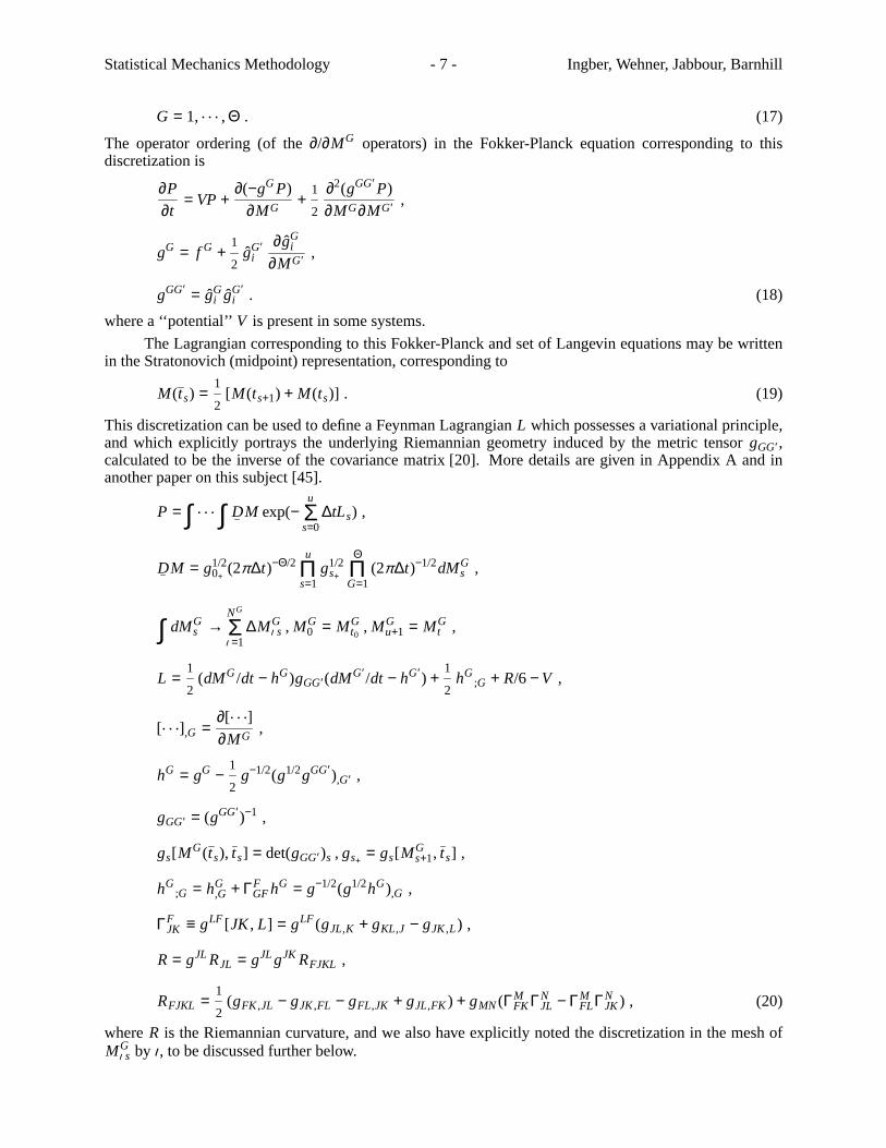
This discretization can be used to define a Feynman LagrangianL which possesses a variational principle,and which explicitly portrays the underlying Riemannian geometry induced by the metric tensorgGG′ ,calculated to be the inverse of the covariance matrix [20]. More details are given in Appendix A and inanother paper on this subject [45].

P = ∫ . . . ∫ DM exp(−u

s=0Σ ∆tLs) ,

DM = g1/20+

(2π∆t)−Θ/2u

s=1Π g1/2

s+

Θ

G=1Π (2π∆t)−1/2dMG

s ,

∫ dMGs →

NG

ι =1Σ ∆MG

ι s , MG0 = MG

t0 , MGu+1 = MG

t ,

L =1

2(dMG/dt − hG)gGG′(dMG′ /dt − hG′) +

1

2hG

;G + R/6 − V ,

[. . .],G =∂[. . .]

∂MG,

hG = gG −1

2g−1/2(g1/2gGG′),G′ ,

gGG′ = (gGG′)−1 ,

gs[MG(ts), ts] = det(gGG′)s , gs+ = gs[M

Gs+1, ts] ,

hG;G = hG

,G + ΓFGFhG = g−1/2(g1/2hG),G ,

ΓFJK ≡ gLF [JK, L] = gLF (gJL,K + gKL,J − gJK,L) ,

R = gJLRJL = gJLgJK RFJKL ,

RFJKL =1

2(gFK ,JL − gJK,FL − gFL,JK + gJL,FK ) + gMN(ΓM

FK ΓNJL − ΓM

FLΓNJK) , (20)

whereR is the Riemannian curvature, and we also have explicitly noted the discretization in the mesh ofMG

ι s by ι , to be discussed further below.


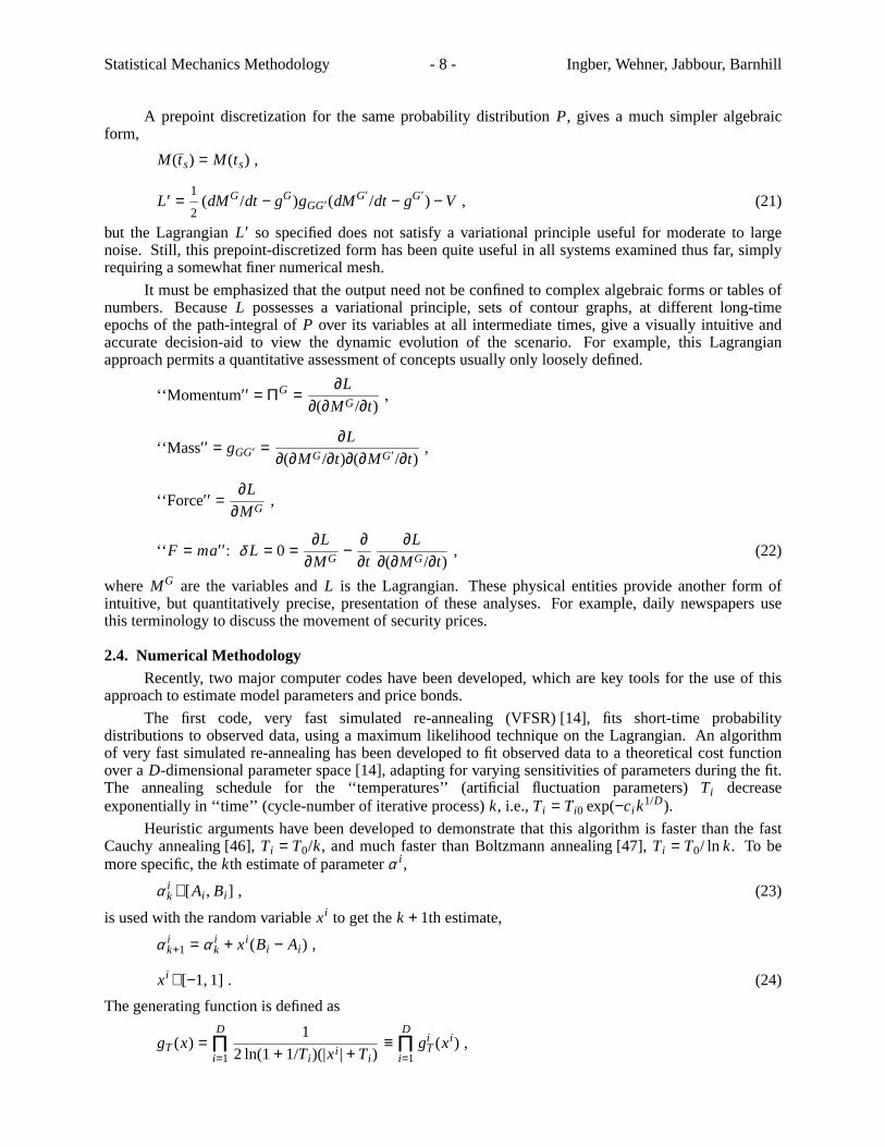
A prepoint discretization for the same probability distributionP, giv es a much simpler algebraicform,

M(ts) = M(ts) ,

L′ =1

2(dMG/dt − gG)gGG′(dMG′ /dt − gG′) − V , (21)

but the LagrangianL′ so specified does not satisfy a variational principle useful for moderate to largenoise. Still, this prepoint-discretized form has been quite useful in all systems examined thus far, simplyrequiring a somewhat finer numerical mesh.

It must be emphasized that the output need not be confined to complex algebraic forms or tables ofnumbers. BecauseL possesses a variational principle, sets of contour graphs, at different long-timeepochs of the path-integral ofP over its variables at all intermediate times, give a visually intuitive andaccurate decision-aid to view the dynamic evolution of the scenario. For example, this Lagrangianapproach permits a quantitative assessment of concepts usually only loosely defined.

‘‘Momentum′′ = ΠG =∂L

∂(∂MG/∂t),

‘‘Mass′′ = gGG′ =∂L

∂(∂MG/∂t)∂(∂MG′ /∂t),

‘‘Force′′ =∂L

∂MG,

‘‘ F = ma′′ : δ L = 0 =∂L

∂MG−

∂∂t

∂L

∂(∂MG/∂t), (22)

where MG are the variables andL is the Lagrangian. These physical entities provide another form ofintuitive, but quantitatively precise, presentation of these analyses. For example, daily newspapers usethis terminology to discuss the movement of security prices.

2.4. Numerical MethodologyRecently, two major computer codes have been developed, which are key tools for the use of this

approach to estimate model parameters and price bonds.

The first code, very fast simulated re-annealing (VFSR) [14], fits short-time probabilitydistributions to observed data, using a maximum likelihood technique on the Lagrangian. An algorithmof very fast simulated re-annealing has been developed to fit observed data to a theoretical cost functionover aD-dimensional parameter space [14], adapting for varying sensitivities of parameters during the fit.The annealing schedule for the ‘‘temperatures’’ (artificial fluctuation parameters)Ti decreaseexponentially in ‘‘time’’ (cycle-number of iterative process)k, i.e.,Ti = Ti0 exp(−ci k

1/D).

Heuristic arguments have been developed to demonstrate that this algorithm is faster than the fastCauchy annealing [46],Ti = T0/k, and much faster than Boltzmann annealing [47],Ti = T0/ ln k. To bemore specific, thekth estimate of parameterα i ,

α ik ∈ [ Ai , Bi ] , (23)

is used with the random variablexi to get thek + 1th estimate,

α ik+1 = α i

k + xi (Bi − Ai ) ,

xi ∈ [−1, 1] . (24)

The generating function is defined as

gT (x) =D

i=1Π 1

2 ln(1+ 1/Ti )(|xi | + Ti )≡

D

i=1Π gi

T (xi ) ,


Ti = Ti0 exp(−ci k1/D) . (25)

Note that the use ofC, the cost function given above, isnot equivalent to doing a simple least squares fiton M(t + ∆t).

The second code develops the long-time probability distribution from the Lagrangian fit by the firstcode. A robust and accurate histogram-based (non-Monte Carlo) path-integral algorithm to calculate thelong-time probability distribution has been developed to handle nonlinear Lagrangians [15,16,48,49],including a two-variable code for additive and multiplicative cases.

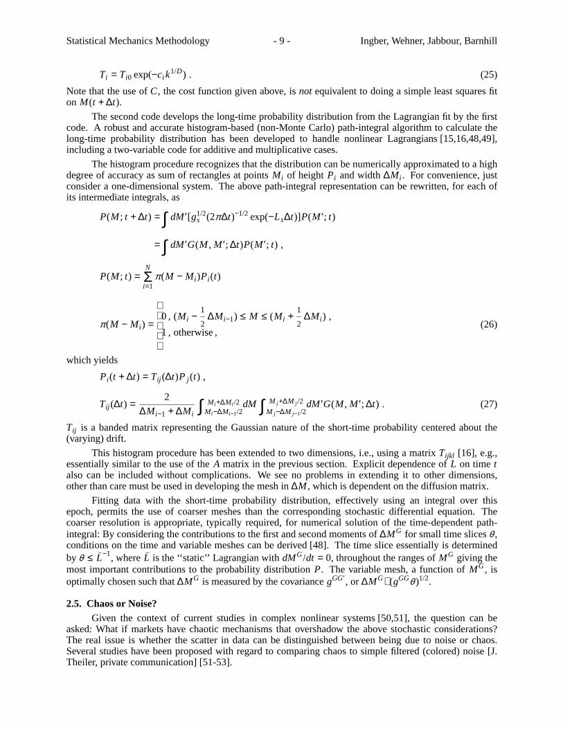
The histogram procedure recognizes that the distribution can be numerically approximated to a highdegree of accuracy as sum of rectangles at pointsMi of heightPi and width∆Mi . For convenience, justconsider a one-dimensional system. The above path-integral representation can be rewritten, for each ofits intermediate integrals, as

P(M ; t + ∆t) = ∫ dM′[g1/2s (2π∆t)−1/2 exp(−Ls∆t)]P(M ′; t)

= ∫ dM′G(M , M ′; ∆t)P(M ′; t) ,

P(M ; t) =N

i=1Σ π(M − Mi )Pi (t)

π(M − Mi ) =

0 , (Mi −1

2∆Mi−1) ≤ M ≤ (Mi +

1

2∆Mi ) ,

1 , otherwise ,(26)

which yields

Pi (t + ∆t) = Tij (∆t)Pj (t) ,

Tij (∆t) =2

∆Mi−1 + ∆Mi∫ Mi+∆Mi /2

Mi−∆Mi−1/2dM ∫ M j +∆M j /2

M j −∆M j−1/2dM′G(M , M ′; ∆t) . (27)

Tij is a banded matrix representing the Gaussian nature of the short-time probability centered about the(varying) drift.

This histogram procedure has been extended to two dimensions, i.e., using a matrixTijkl [16], e.g.,essentially similar to the use of theA matrix in the previous section. Explicit dependence ofL on timetalso can be included without complications. We see no problems in extending it to other dimensions,other than care must be used in developing the mesh in∆M , which is dependent on the diffusion matrix.

Fitting data with the short-time probability distribution, effectively using an integral over thisepoch, permits the use of coarser meshes than the corresponding stochastic differential equation. Thecoarser resolution is appropriate, typically required, for numerical solution of the time-dependent path-integral: By considering the contributions to the first and second moments of∆MG for small time slicesθ ,conditions on the time and variable meshes can be derived [48]. The time slice essentially is determinedby θ ≤ L−1, whereL is the ‘‘static’’ Lagrangian withdMG/dt = 0, throughout the ranges ofMG giving themost important contributions to the probability distributionP. The variable mesh, a function ofMG, isoptimally chosen such that∆MG is measured by the covariancegGG′ , or ∆MG∼ (gGGθ )1/2.

2.5. Chaos or Noise?Given the context of current studies in complex nonlinear systems [50,51], the question can be

asked: What if markets have chaotic mechanisms that overshadow the above stochastic considerations?The real issue is whether the scatter in data can be distinguished between being due to noise or chaos.Several studies have been proposed with regard to comparing chaos to simple filtered (colored) noise [J.Theiler, private communication] [51-53].


The previous references must be generalized, such that we must investigate whether scatter inmarkets’ data can be distinguished from multiplicative noise. A previous application of this methodologyfollows:

One of us (LI) was principal investigator of a US Army Models Committee project, working with ateam of Army and Lawrence Livermore National Laboratory personnel to compare, for the first time,large-scale high-fidelity combat computer-model data to exercise data [16,41]. The combat analysis waspossible only because now we had recent data on combat exercises from the National Training Center(NTC) of sufficient temporal density to attempt dynamical mathematical modeling. The criteria used to(not) determine chaos in this dynamical system is the nature of propagation of uncertainty, i.e., thevariance. For example, following by-now standard arguments [J. Yorke, seminar and privatecommunication], propagation of uncertainty may be considered as (a) diminishing, (b) increasingadditively, (c) or increasing multiplicatively. An example of (a) is the evolution of a system to anattractor, e.g., a book dropped onto the floor from various heights reaches the same point no matter whatthe spread in initial conditions. An example of (b) is the propagation of error in a clock, a cyclic system.Examples of (c) are chaotic systems, of which very few real systems have been shown to belong. Anexample of (c) is the scattering of a particle in a box whose center contains a sphere boundary: When aspread of initial conditions is considered for the particle to scatter from the sphere, when its trajectoriesare aligned to strike the sphere at a distance from its center greater that the diameter, the spread inscattering is a factor of about three greater than the initial spread.

In our analysis of NTC data, we were able to fit the short-time attrition epochs (determined to beabout 5 minutes from mesh considerations determined by the nature of the Lagrangian) with short-timenonlinear Gaussian-Markovian probability distributions with a resolution comparable to the spread indata. When we did the long-time path-integral from some point at the beginning of the battle, we foundthat we could readily find a form of the Lagrangian that made physical sense and that also fit themultivariate variances as well as the means at each point in time of the rest of the combat interval. I.e.,there was not any degree of hyper-sensitivity to initial conditions that prevented us from ‘‘predicting’’ thelong time means and variances of the system. Since the system is dissipative, there is a strong tendencyfor all moments to diminish in time, but in fact this combat is of sufficiently modest duration (typically 1to 2 hours) that variances do increase somewhat during the middle of the battle. In summary, thisbattalion-regiment scale of this particular battle did not seem to possess chaos.

Similar considerations and calculations are planned for these studies of financial markets.

3. BRENNAN-SCHWARTZ MODELS

3.1. Interest RatesThe pioneering Brennan-Schwartz (BS) model [5,7] can be used to illustrate how this methodology

is to be implemented numerically.

The BS model is summarized by:

dr = [a1 + b1(l − r )]dt + rσ1dz1 ,

dl = [l (a2 + b2r + c2l )]dt + lσ2dz2 ,

< dzi >= 0 , i = {1, 2} ,

< dzi (t)dzj (t ′) >= dtδ (t − t ′) , i = j ,

< dzi (t)dzj (t ′) >= ρdtδ (t − t ′) , i ≠ j ,

δ (t − t ′) =

0 , ,

1 ,

t ≠ t ′ ,

t = t ′ ,(28)

where < . > denotes expectations.


These can be rewritten as Langevin equations (in the Itoˆ prepoint discretization)

dr/dt = a1 + b1(l − r ) + σ1r (γ +n1 + sgnρ γ −n2) ,

dl/dt = l (a2 + b2r + c2l ) + σ2l (sgnρ γ −n1 + γ +n2) ,

γ ± =1

√ 2[1 ± (1 − ρ2)1/2]1/2 ,

ni = (dt)1/2pi , (29)

wherep1 and p2 are independent [0,1] Gaussian distributions.

The cost functionC is defined from the equivalent short-time probability distribution,P, for theabove set of equations.

P = g1/2(2πdt)−1/2 exp(−Ldt)

= exp(−C) ,

C = Ldt +1

2ln(2πdt) − ln(g) ,

L =1

2F†gF ,

F =

dr/dt − ((a1 + b1(l − r )))

dl/dt − l (a2 + b2r + c2l )

,

g = det(g) ,

k = 1 − ρ2 . (30)

g, the metric in{ r , l } -space, is the inverse of the covariance matrix,

g−1 =

(rσ1)2

ρrlσ1σ2

ρrlσ1σ2

(lσ2)2

. (31)

As discussed above, the correct mesh for time,dt, in order thatP represent the Langevin equations (toorderdt3/2) is

dt ≤ 1/L , (32)

whereL is L evaluated withds/dt = dl/dt = 0. If dt is greater than 1/L, then it is inappropriate to useP,and instead the path integral over intermediate states of folded short-time distributions must be calculated.In this context, it should be noted that the correct time mesh for the corresponding differential equationsmust be at least as small, since typically differentiation is a ‘‘sharpening’’ process. This will be noted inany discipline requiring numerical calculation, when comparing differential and integral representationsof the same system.

The VFSR code was checked out with a rather stringent test: Data was ‘‘generated’’ using the BSequations above as asimulation, using a set of parameters given in the 1982 BS paper. Then, theLagrangian was used as a cost function to search for the parameters used in the generation of the data. Atime mesh was established at each point in time using the criteria given above, which turns out to bedt ∼ 1 day. The code converged to within the statistical accuracy of the generated data. When a timemesh ofdt = 1 month was used, as did BS, the results did not match the simulated data.

In light of the above, it should not be surprising that computer runs with real Treasury bills andbonds over the same epochs as BS, using end-of-month data, did not agree precisely with BS or withsimilar runs using daily data. Note we are not using the exact data as BS. However, should we be


concerned about the lack of excellent convergence with BS? As determined fromC′ above, thedt ∼ 1day, possibly 1 week, is appropriate to use to define the short-time probability distribution, data notavailable in the 1982 BS study.

However,dt ∼ 1 day, not available for the BS work, shows marked deviations in the development ofinterest variables for selected trajectories using the BS equations as a simulation of data. This suggeststhat a two-state model is insufficient to capture faster movements in rates at the daily scale.

When the s.d.e. were permitted to evolve, trajectories developed increasing interest rates. It wasnoted that when the rates approached 100%, there suddenly was extremely wild growth of these variables.In the context of chaos discussed above, this region will be further investigated.

3.2. Security PricesBS [5] present arguments recognizing that the stochastic price of a discount bond for a given

maturity dateT can utilize straightforward stochastic calculus to derive a form in terms of coefficientsappearing in theirr − l coupled stochastic equations. They use arbitrage arguments on portfolios of bondswith different maturity dates to derive zero risk conditions for the market prices of risks,λ 1 andλ 2, forshort-term and long-term interest rates, respectively. By consideringl as related to a bond’s price, theystraightforwardly derive an arbitrage expression forλ 2. Their resulting partial differential equation(p.d.e.) is an equilibrium (mean value) equation for a pure discount-bond priceB, at a giv en time untilmaturityτ = T − t and ‘‘continuous’’ coupon payment ofc.

The above formulation of interest rates is used by BS to determine the parameters needed tocalculate their derived p.d.e. for securities, i.e., bond pricesB. Using some notation developed above,with { MG; G = r , l } , they obtain

∂B

∂τ= VB+

∂(−gGB)

∂MG+

1

2

∂2(gGG′ B)

∂MG∂MG′ ,

gr = −(β1 − λ 1η1)

= −a1 − b1(l − r ) + λ 1rσ1 ,

gl = −(β2 − λ 2η2)

= −l (σ 22 + l − r ) ,

(gGG′) = (g)−1 ,

V =c

B− r , (33)

wherec is the continuous coupon rate for bondB, andλ 1 is an additional parameter to be fit by the data.

The above equation represents a ‘‘truly nonlinear’’ Fokker-Planck equation because of the presenceof B in V. Howev er, ifc/B is a smooth function, such that

V(MG; τ ′) − V(MG; τ )

ε= ∆τ

∂V

∂τ+ ∆τ ∫

δV

δ B

∂B(M ′G′)

δ τdM′G′

= O(∆τ ν ) , (34)

for ν > 1, whereτ ′ = τ + ε∆τ , then our numerical path-integral codes may be used here as well [15].

In this formulation, all the above algebraic and numerical methodology can be utilized to define aLagrangian-like function,LB, defining the evolution ofB, subject to whatever initial conditions andboundary conditions are deemed appropriate, e.g., if considering bonds or options [7,9]. Care must betaken with the discretization in the forwardτ direction.


In particular, it was tempting to use our simulated-annealing codes to fitLB; then our path-integralcodes can be used to evolve/predictB for long epochs. The use ofLB as a cost function for fitting data isstill reasonable even thoughB is not abona fideE.g., B is hypothesized to be determined by intensearbitrage, in the derivation of the p.d.e. This is equivalent to stating that the process is confined, withinstatistical fluctuations, to a maximum likelihood path. This is mathematically articulated in ourmethodology as stating that the variational principle associated (not independently assumed) withLB,including the specification of the boundary conditions and initial conditions, implies that we can fit thevariables inLB to data specified by observed values. This is numerically similar to the way we perform amaximum likelihood fit of the Lagrangian associated with the s.d.e. As we show below, this assumptionappears to be well supported in our fits ofLB to observedr − l data, in that we get a set parameters veryclose to those obtained by fitting theL associated with the s.d.e. It should be noted that BS calculatedtheir λ 1 by interpolating fits to bond prices, thereby incorporating lots of pricing information intoλ 1.

However, independent of such arguments, once the parameters are established, it is mathematicallycorrect to use our path-integral codes on theB equation, with its initial conditions and boundaryconditions, to calculate the long-time evolution ofB.

We note that our use ofLB to describe the evolution ofB is similar in spirit to recent attempts todescribe the evolution of bond prices as a functional of forward rates, for example by Heath, Jarrow andMorton (HJM) [18,19]. Our functional corresponding to theirs is simply the LagrangianLB. HJMdevelop arbitrage arguments to impose equilibrium evolution by randomly varying their interest-ratefunctional, somewhat similar to the numerical importance-sampling methodology employed whenperforming numerical Monte Carlo techniques to take advantage of an underlying variationalprinciple [14,54]. The trade-off in dev eloping a theory of stochastic forward pricing is that parabolicequations are unstable for the negative diffusion in calendar timet so defined for financial systems, and soHJM must impose additional constraints to prevent this explosion. The BS technique of developingB asa function ofτ = T − t avoids these problems. The methodology of HJM does not require the separateestimation of market risk factors, e.g.,λ 1. Our Lagrangian representation of the BS model, coupled withour arbitrage arguments, also permits us to fit all parameters directly to interest rate data. Themethodology of HJM permits the introduction of colored (time delayed) noise, which also can beincluded in our methodology, albeit with substantial effort. In principle, given a forward rate HJM modelfor a Lagrangian, then all our methodology could be used here as well.

In many cases it may be of interest to study the stochastic systems of interest rates, e.g., the coupledr − l equations above. Howev er, if only the evolution ofB is of interest, then it is more direct, and likelymore numerically accurate, to fit the parameters in the cost functionCB (derived from LB as C wasderived fromL above). I.e., we fit{ a1, b1, ρ,σ2, λ 1} to { r , l , B, c} data. Since, as discussed below, wewill be dealing with portfolios of pure discount bonds to represent coupon bonds, we considerc = 0,thereby requiring only{ r , l } data. We do not need the parameters{ a2, b2, c2} because of the arbitragearguments used to calculateβ2 − λ 2η2 above [3]. This greatly improves the statistical merit of our fits,requiring two less degrees of freedom for theB equation. This approach also may be viewed as anempirical test of the consistency of assumptions used to derive the bond equation. Our VFSRmethodology also explicitly include boundary conditions, a very important component of any model evenif only implicitly described, since we use the same cost function, but as a function of its variables insteadof its parameters, to calculate the evolution of bond prices with the path integral.

The ultimate test of any methodology is to compare theoretical predictions/descriptions withobserved data [55]. Assume we already have fit our parameters for the entire epoch of interest. Actualbond prices with coupons may then be evaluated straightforwardly by considering a portfolio ofn purediscount bonds with a series of maturity datesTn equivalent to the dates of payment of coupons and theface value of the actual coupon bond to be modeled. This prescription requires that we integrate backsuch a portfolio ofn pure discount bonds with maturityTn, to various timesti < T (including only thosebonds in the portfolio with maturityTn ≥ ti ). At each of these times, we use the observed values ofr (ti )and l (ti ) to calculate the bond pricesBn(ti ). This portfolio of{ Bn(ti )} is then compared to the observedcoupon bondB(ti ), i.e., for many such times{ ti } . For each zero-coupon bond in this portfolio, we start atits time of maturityTn, enforcing the initial conditionsBn(r , l ; Tn) = 1, and integrate back to a given timet < Tn. We then weight each zero coupon bond by the actual coupon or face value paid on the coupon


bond.

Similarly, for the important purpose of theoretically pricing an actual coupon bond at timet, we usethe same methodology, e.g., using the present day’s best estimate ofr (t) andl (t) to calculateB(r , l ; t).

We are not in complete agreement with BS on their use of boundary conditions and numericalimplementation [5]. Their use of ‘‘natural’’ boundary conditions, actually more general unrestricted orsingular boundary conditions [56], is in part based on their own admittedlyad hocchoice of functionalforms forr andl diffusions, in both their s.d.e. and p.d.e., and in ther drift in their s.d.e. We believe thatthe appropriate boundary conditions must be determined by finance considerations as follows:

r → 0 and l → 0 turn out to be natural boundary conditions of their model being inaccessible inany finite time, and therefore do not require or permit any additional specification. Atr = 0, we shouldhaveB(t + ∆t) = B(t), i.e., reflecting boundary conditions. This is the regular boundary conditions of themodel only if ther drift is greater than zero [49,56]. Atl = 0, the BS model yields a unrestrictedboundary conditions implyingB = 0, and therefore does not require or permit any additional specification.Further examination shows thatl = 0 is sometimes an entrance condition, sometimes an exit condition,depending on the value ofr . Similar analyses show thatr → ∞ and l → ∞ also are unrestrictedboundary conditions.

For ther drift in the s.d.e. and in the p.d.e. to be non-negative, it is necessary, not sufficient, thata1 ≥ 0. We therefore propose thata1 be constrained to achieve only these values in the fit. As mentionedin the introduction, BS also prefer this constraint ona1. This may be considered a constraint just as is thefunctional form of the model. As it turned out, to be discussed below, the value ofa1 we obtained in ourfit was essentially zero.

In setting up the path integral for the BSB p.d.e., we use all natural boundary conditions. Thisimplies that there is no freedom to choose or to redundantly impose boundary conditions as we believedid BS. We choose the simple free-space Gaussian short-time propagator, since the evolution ofB cannotleave the enclosed boundary conditions, since it is the proper solution deep in the interior ofr − l space,and since the drift is benign to the extent that this also is a good solution at the boundaries to order∆τ 3/2 [15,48,49].

Since the boundary conditions atr = 0 and l = 0 are mathematically unrestricted if the diffusionsvanish at these boundaries, as they do for the BS model, we therefore also propose that thead hocfunctional form of the diffusions be relaxed to admit additive noise components, e.g.,κ 1 andκ 2. This isespecially important forr = 0. This not only can be tested by so fitting data, but also mathematicallypermits the imposition of external boundary conditions more tightly constrained to the financial systemunder consideration, not being technically restricted by the actual functional forms chosen for the driftsand diffusions. Thus we also tested models for which

rσ1 → rσ1 +κ 1 ,

lσ2 → lσ2 +κ 2 , (35)

in the drifts and diffusions of the bond p.d.e. Because of the induced singular behavior in thel -drift, thistransformation still requires unrestricted boundary conditions atl = 0, which turn out to be entranceboundary conditions.

We believe it is extremely important to gain this freedom over the functional forms of the drifts anddiffusions. For example, our calculations with this model clearly demonstrate that the rather mildnonlinearities of the BS model only permit inflationary evolution, since those were the periods were fit todata and since the functional forms likely cannot accommodate many swings and dips, on time scales ofmonths or years, much longer that of the fluctuations, yet shorter than the period of long-term bonds.This appears to require a higher degree of nonlinearity and/or an increase in the number of independentinterest-rate variables.

For future calculations, we propose to include some additive components in ther and l diffusions.We intend to invoke external reflecting boundary conditions forr = 0, using the method of images.Similar sets of boundary conditions were used in a previous project [16]. We checked the accuracy of thereflecting boundary conditions using MACSYMA, an algebraic manipulator.


BS procedures used a discretized form of their p.d.e. They compared their theoretical and observedvalues ofB for several values ofλ 1, and interpolated to find the best value ofλ 1 which fit the data. Ourmethodology of calculatingλ 1 from LB, simultaneously with the other parameters in the p.d.e., avoidsthis additional step in their methodology.

4. NUMERICAL RESULTS

4.1. Fits to Interest RatesInterest rates were developed from Treasury bill and bond yields during the period October 1974

through December 1979, the same period as one of the sets used by BS [7]. Short-term rates weredetermined from Treasury bills with a maturity of three months (BS used 30-day maturities), and long-term rates were determined from Treasury bonds with a maturity of twenty years (BS used at least 15-yearmaturities). For monthly runs, we used 63 points of data between 74-10-31 and 79-12-28. For daily runs,we used 1283 points of data between 74-10-31 and 79-12-31. We used yearly rates divided by 12 to fitthe parameters.

For daily data, the actual number of days between successive trades was used; i.e., during this timeperiod we had 1282 pieces of daily data and 62 pieces of end-of-month data. Although a rescaling in timeonly simply scales the deterministic parameters linearly, since that is how they appear in this model, thisis not true forρ. Then we did all subsequent runs using the scale of one day. We used yearly ratesdivided by 365 to fit the parameters.

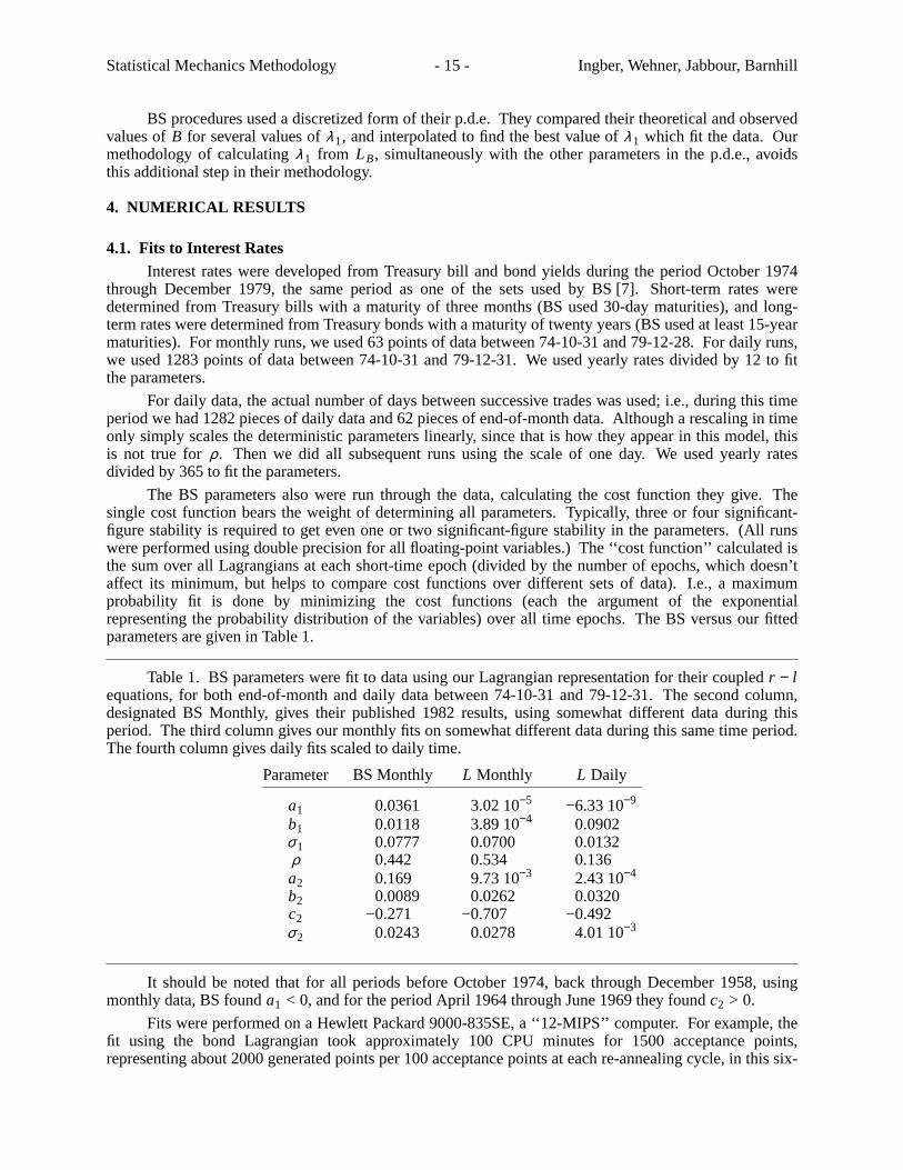
The BS parameters also were run through the data, calculating the cost function they giv e. Thesingle cost function bears the weight of determining all parameters. Typically, three or four significant-figure stability is required to get even one or two significant-figure stability in the parameters. (All runswere performed using double precision for all floating-point variables.) The ‘‘cost function’’ calculated isthe sum over all Lagrangians at each short-time epoch (divided by the number of epochs, which doesn’taffect its minimum, but helps to compare cost functions over different sets of data). I.e., a maximumprobability fit is done by minimizing the cost functions (each the argument of the exponentialrepresenting the probability distribution of the variables) over all time epochs. The BS versus our fittedparameters are given in Table 1.

Table 1. BS parameters were fit to data using our Lagrangian representation for their coupledr − lequations, for both end-of-month and daily data between 74-10-31 and 79-12-31. The second column,designated BS Monthly, giv es their published 1982 results, using somewhat different data during thisperiod. The third column gives our monthly fits on somewhat different data during this same time period.The fourth column gives daily fits scaled to daily time.

Parameter BS Monthly L Monthly L Daily

a1 0.0361 3.02 10−5 −6.33 10−9

b1 0.0118 3.89 10−4 0.0902σ1 0.0777 0.0700 0.0132ρ 0.442 0.534 0.136a2 0.169 9.73 10−3 2.43 10−4

b2 0.0089 0.0262 0.0320c2 −0.271 −0.707 −0.492σ2 0.0243 0.0278 4.01 10−3

It should be noted that for all periods before October 1974, back through December 1958, usingmonthly data, BS founda1 < 0, and for the period April 1964 through June 1969 they foundc2 > 0.

Fits were performed on a Hewlett Packard 9000-835SE, a ‘‘12-MIPS’’ computer. For example, thefit using the bond Lagrangian took approximately 100 CPU minutes for 1500 acceptance points,representing about 2000 generated points per 100 acceptance points at each re-annealing cycle, in this six-


dimensional parameter space. It was found that once the VFSR code repeated the lowest cost functionwithin two cycles of 100 acceptance points, e.g., typically achieving 3 or 4 significant-figure accuracy inthe global minimum of the cost function, by shunting to a local fitting procedure, the Broyden-Fletcher-Goldfarb-Shanno (BFGS) algorithm [57], only several hundred acceptance points were required toachieve 7 or 8 significant-figure accuracy in the cost function. This also provided yet another test of theVFSR methodology.

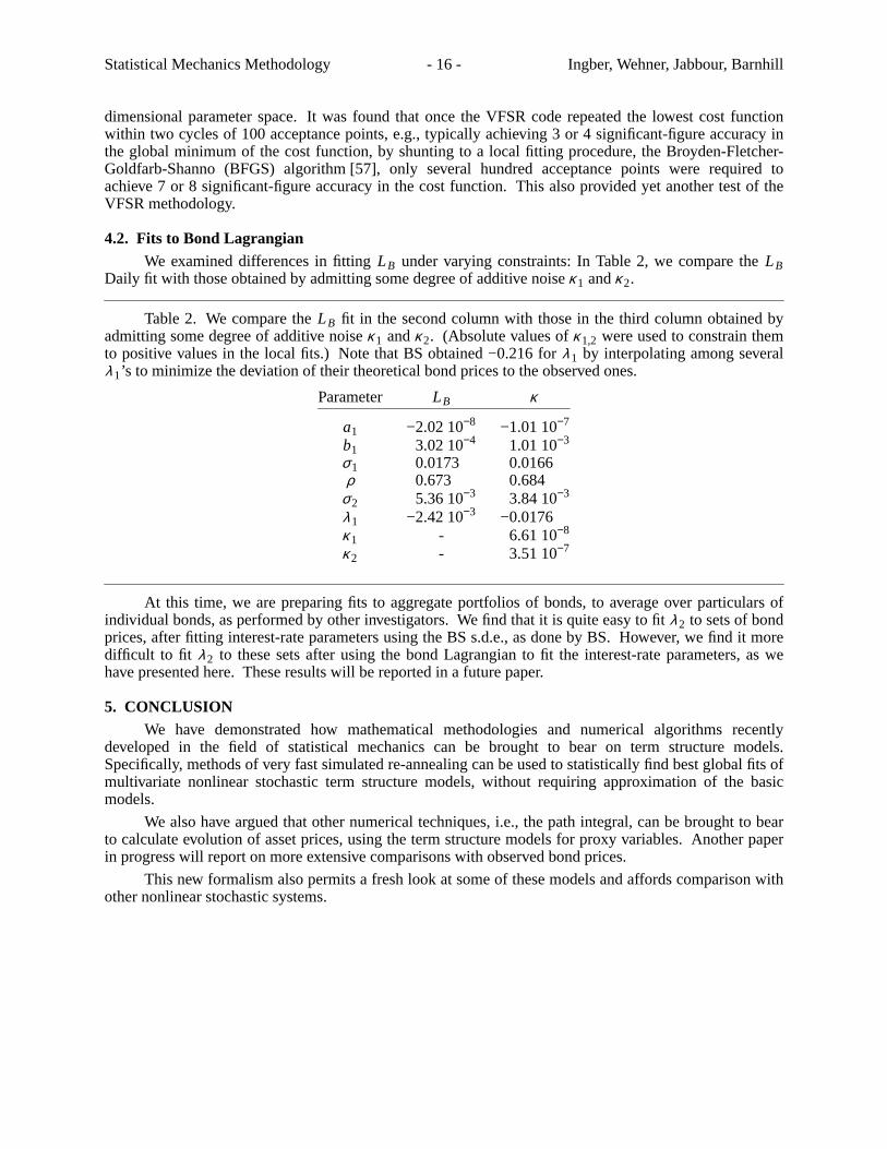
4.2. Fits to Bond LagrangianWe examined differences in fittingLB under varying constraints: In Table 2, we compare theLB

Daily fit with those obtained by admitting some degree of additive noiseκ 1 andκ 2.

Table 2. We compare theLB fit in the second column with those in the third column obtained byadmitting some degree of additive noiseκ 1 andκ 2. (Absolute values ofκ 1,2 were used to constrain themto positive values in the local fits.) Note that BS obtained −0.216 forλ 1 by interpolating among severalλ 1’s to minimize the deviation of their theoretical bond prices to the observed ones.

Parameter LB κ

a1 −2.02 10−8 −1.01 10−7

b1 3.02 10−4 1.01 10−3

σ1 0.0173 0.0166ρ 0.673 0.684

σ2 5.36 10−3 3.84 10−3

λ 1 −2.42 10−3 −0.0176κ 1 - 6.61 10−8

κ 2 - 3.51 10−7

At this time, we are preparing fits to aggregate portfolios of bonds, to average over particulars ofindividual bonds, as performed by other investigators. We find that it is quite easy to fitλ 2 to sets of bondprices, after fitting interest-rate parameters using the BS s.d.e., as done by BS. However, we find it moredifficult to fit λ 2 to these sets after using the bond Lagrangian to fit the interest-rate parameters, as wehave presented here. These results will be reported in a future paper.

5. CONCLUSIONWe hav e demonstrated how mathematical methodologies and numerical algorithms recently

developed in the field of statistical mechanics can be brought to bear on term structure models.Specifically, methods of very fast simulated re-annealing can be used to statistically find best global fits ofmultivariate nonlinear stochastic term structure models, without requiring approximation of the basicmodels.

We also have argued that other numerical techniques, i.e., the path integral, can be brought to bearto calculate evolution of asset prices, using the term structure models for proxy variables. Another paperin progress will report on more extensive comparisons with observed bond prices.

This new formalism also permits a fresh look at some of these models and affords comparison withother nonlinear stochastic systems.


APPENDIX A: STATISTICAL MECHANICS DERIVATION OF PATH INTEGRAL

This Appendix outlines the derivation of the path integral representation of the nonlinear Langevinequations, via the Fokker-Planck representation. This serves to point out the importance of properlytreating nonlinearities, and to emphasize the deceptive simplicity of the Langevin and Fokker-Planckrepresentations of stochastic systems. There are a few derivations in the literature, but the following blendseems to be the most concise. All details may be found in the references given in this paper [23,58-60].

The Stratonovich (midpoint discretized) Langevin equations can be analyzed in terms of the Wienerprocess dWi , which can be rewritten in terms of Gaussian noiseη i = dWi /dt if care is taken in thelimit [23].

dMG = f G[t, M(t)]dt + gGi [t, M(t)]dWi ,

MG(t) = f G[t, M(t)] + gGi [t, M(t)]η i (t) ,

dWi → η idt ,

M = { MG; G = 1,. . . , Λ} ,

η = {η i ; i = 1,. . . , N} .

MG = dMG/dt ,

< η j (t) >η = 0 ,

< η j (t),η j ′(t ′) >η = δ jj ′δ (t − t ′) , (A.1)

η i represents Gaussian white noise, and moments of an arbitrary functionF(η ) over this stochastic spaceare defined by a path-type integral overη i ,

< F(η ) >η = N−1 ∫ Dη F(η ) exp(−1

2

∞

t0∫ dtη iη i ) ,

N = ∫ Dη exp(−1

2

∞

t0∫ dtη iη i ) ,

Dη =v→∞lim

v+1

α =0Π

N

j=1Π (2πθ)−1/2dW j

α ,

tα = t0 + αθ ,

1

2 ∫ dtη iη i =1

2θ βΣ

iΣ (Wi

β − Wiβ−1)2 ,

< η i >η = 0 ,

< η i (t)η j (t ′) >η = δ ij δ (t − t ′) . (A.2)

Non-Markovian sources,η , and their influence throughout this development, can be formallytreated by expansions about the Markovian process by defining

< F(η ) >η = N−1ξ ∫ Dη F exp[−

1

2 ∫ ∫ dtdt ′η (t)∆−1ξ (t − t ′)η (t ′)] ,


∫ dt ∆−1ξ (t − t ′)∆ξ (t ′ − t ′′ ) = δ (t − t ′′ ) , (A.3)

with ξ defined as an interval centered about the argument of∆ξ . Letting ξ → 0 is an unambiguousprocedure to define the Stratonovich prescription used below.

In terms of a specific stochastic pathη , a solution to Eq. (A.1),MGη (t; M0, t0) with

MGη (t0; M0, t0) ≡ M0, the initial conditions on the probability distribution ofMη is

Pη [M , t|M0, t0] = δ [M − Mη (t; M0, t0)] . (A.4)

Using the conservation of probability condition,

Pη ,t + (MGPη ),G = 0 ,

[. . .],G = ∂[. . .]/∂MG ,

[. . .],t = ∂[. . .]/∂t , (A.5)

the evolution ofPη is written as

Pη ,t [M , t|M0, t0] = { [− f G(t, M) − g(t, M)η i ]Pη } ,G . (A.6)

To perform the stochastic average of Eq. (A.6), the ‘‘functional integration by parts lemma’’ [28] isused on an arbitrary functionZ(η ) [59],

∫ Dηδ Z(η )

δ η i= 0 . (A.7)

Applied toZ = Z′ exp(−1

2 ∫∞t0

dtη iη i ), this yields

< η i Z′ >η =< δ Z′/δ η i >η . (A.8)

Applying this toF [Mη ] = ∫ dM Pη F(M),

∫ dMδ Pη

δ η iF(M) =

∂F [Mη ]

∂MGη

δ MGη

δ η i

= −1

2 ∫ dM F(M)( gGj δ ij Pη ),G , (A.9)

whereδ designates functional differentiation. The last equation has used the Stratonovich prescription,

MGη (t) = MG

0 + ∫ dt ′ H(t − t ′)H(t − t0)( f G + gGi η i ) ,

t ′→t−0lim

δ MGη (t)

δ η i (t ′)=

1

2gG

j [t, Mη (t)]δij ,

H(z) =

1, z ≥ 0

0, z < 0 .(A.10)

Taking the averages <Pη ,t >η and <η i Pη >η , the Fokker-Planck is obtained from Eq. (A.9). Ifsome boundary conditions are added as Lagrange multipliers, these enter as a ‘‘potential’’V, creating aSchrodinger-type equation.

P,t =1

2(gGG′ P),GG′ − (gGP),G + VP ,

P =< Pη >η ,


gG = f G +1

2gG′

i gGi ,G′ ,

gGG′ = gGi gG′

i ,

[. . .],G = ∂[. . .]/∂MG . (A.11)

Note thatgG replaces f G in Eq. (A.1) if the Ito(prepoint discretized) calculus is used to define thatequation.

To derive the path integral representation of Eq. (A.11), define operatorsMG

, pG andH ,

[MG

, pG′ ] ≡ MG

pG′ − pG′ MG = iδ G

G′ ,

[MG

, MG′

] = 0 = [ pG, pG′ ] ,

P,t = −i H P ,

H = −i

2pG pG′ g

GG′ + pGgG + iV , (A.12)

and define the evolution operatorU(t, t ′) in terms of ‘‘bra’’ and ‘‘ket’’ probability states ofM ,

MG

|MG >= MG|MG > ,

pG|MG >= −i∂/∂MG|MG > ,

< M ′|M >= δ (M ′ − M) ,

< M |p >= (2π)−1 exp(ip ⋅ M) ,

P[M , t|M0, t0] =< M |U(t, t0)|M0 > ,

H(t ′)U(t ′, t) = iU (t ′, t),t ′ ,

U(t, t) = 1 ,

U(tρ , tρ−1)≈1 − iθ H(tρ−1) , (A.13)

where ρ indexes units ofθ measuring the time evolution. This is formally integrated to give the pathintegral in the phase space (p, M),

P[Mt |M0] =M(t)=Mt

M(t0)=M0

∫ DM Dp exp[t

t0∫ dt ′(ipGMG −

1

2pG pG′ g

GG′ − ipGgG + V) ] ,

DM =u→∞lim

GΠ

u

ρ=1Π dMG

ρ ,

Dp =u→∞lim

GΠ

u+1

ρ=1Π (2π)−1dpGρ ,

tρ = t0 + ρθ . (A.14)

The integral over each dpGρ is a Gaussian and simply calculated. This gives the path integral incoordinate spaceM , in terms of the prepoint discretized Lagrangian,


P[Mt |M0] = ∫ DMu

ρ=0Π (2πθ)−Λ/2g(Mρ , tρ)1/2

×exp{ −1

2θ gGG′(Mρ , tρ)[∆G

ρ /θ − gG(Mρ , tρ)]

×[∆G′ρ /θ − gG′(Mρ , tρ)] + θV(Mρ , tρ)} ,

LI (MG, MG, t) =

1

2(MG − gG)gGG′(M

G′ − gG′) − V ,

g = det(gGG′) ,

gGG′ = (gGG′)−1 ,

∆Gρ = MG

ρ+1 − MGρ . (A.15)

This can be transformed to the Stratonovich representation, in terms of the Feynman LagrangianLpossessing a covariant variational principle,

P[Mt |M0] = ∫ DMu

ρ=0Π (2πθ)−Λ/2g(Mρ + ∆ρ , tρ + θ /2)1/2

×exp{ − min

tρ+θ

tρ

∫ dt ′L[M(t ′), M(t ′), t ′] } , (A.16)

where ‘‘min’’ specifies that Eq. (A.11) is obtained by constrainingL to be expanded about thatM(t)which makes the actionS = ∫ dt ′L stationary forM(tρ) = Mρ andM(tρ + θ ) = Mρ+1.

One way of proceeding is to expand Eq. (A.15) and compare to Eq. (A.16), but it is somewhateasier to expand Eq. (A.16) and compare to Eq. (A.15) [60]. It can be shown that expansions to orderθsuffice, and that∆2 = O(θ ).

Write L in the general form

L =1

2gGG′ M

GMG′ − hGMG + b

= L0 + ∆L ,

L0 =1

2gGG′ [M(t), t]MGMG′ ,

gGG′ [M(t), t] = gGG′ [M(t), t ′] + gGG′,t ′ [M(t), t ′](t − t ′) + O[(t − t ′)2] , (A.17)

wherehG andb must be determined by comparing expansions of Eq. (A.15) and Eq. (A.16). Only theL0

term is dependent on the actualM(t) trajectory, and sotρ+θ

tρ

∫ dt ∆L = (1

4gGG′,t∆G∆G′ − hG∆G −

1

2hG,G′∆G∆G′ + θ b)|(M ,t) , (A.18)

where ‘‘ |(M ,t)’’ implies evaluation at (M , t).

The determinantg is expanded as

g(M + ∆, t + θ /2)1/2≈g1/2(M , t) exp[θ4g

g,t +1

2g∆Gg,G


+1

4g∆G∆G′(g,GG′ + g−1g,Gg,G′)]|(M ,t) . (A.19)

The remaining integral overL0 must be performed. This is accomplished using the variationalprinciple applied to∫ L0 [58],

gGH M H = −1

2(gGH,K + gGK,H − gKH ,G)M K M H ,

M F = −ΓFJK M J M K ,

ΓFJK == gLF [JK, L] = gLF (gJL,K + gKL,J − gJK,L) ,

(1

2gGH MGM H ),t = 0 ,

t+θ

t∫ L0dt≈

θ2

gGH MGM H |(M ,t+θ ) . (A.20)

Differentiating the second equation in Eq. (A.20) to obtain...M , and expandingM(t + θ ) to third order inθ ,

M(t + θ ) = [1

θ∆G −

1

2θΓG

KL∆K ∆L +1

6θ(ΓG

KL,N + ΓGANΓ A

KL)∆G∆L∆N ]|(M ,t) . (A.21)

Now Eq. (A.16) can be expanded as

P[Mt |M0]dM(t) = ∫ DMu

ρ=0Π exp[−

1

2θgGG′(M , t)∆G∆G′ + B] ,

DM =u+1

ρ=1Π g1/2

ρGΠ (2πθ)−1/2dMG

ρ . (A.22)

Expanding expB to O(θ ) requires keeping terms of order∆, ∆2, ∆3/θ , ∆4/θ , and∆6/θ2. Under the pathintegral, evaluated at (M , t), and using ‘‘=’’ to designate the order of terms obtained from

∫ d∆ ∆n exp(−1

2θ∆2),

∆G∆H = θ gGH ,

∆G∆H∆K = θ (∆GgHK + ∆H gGH + ∆K gGH) ,

∆G∆H∆A∆B = θ2(gGH gAB + gGAgHB + gGBgHA) ,

∆A∆B∆C∆D∆E∆F = θ3(gABgCDgEF + 14 permutations) . (A.23)

This expansion of expB is to be compared to Eq. (A.15), expanded as

P[Mt |M0]dM(t)≈ ∫ DMu

ρ=0Π exp(−

1

2θgGG′∆G∆G′)

×[1 + gGG′ gG∆G′ + θV + O(θ3/2)] , (A.24)

yielding identification ofhG andb in Eq. (A.16),

hG = gGG′ hG′ = gG −1

2g−1/2(g1/2gGG′),G′ ,


b =1

2hGhG +

1

2hG

;G + R/6 − V ,

hG;G = hG

,G + ΓFGFhG = g−1/2(g1/2hG),G ,

R = gJLRJL = gJLgFK RFJKL . (A.25)

The result is

P[Mt |Mt0]dM(t) = ∫ . . . ∫ DM exp(−mint

t0∫ dt ′L)δ [M(t0) = M0]δ [M(t) = Mt ] ,

DM =u→∞lim

u+1

ρ=1Π g1/2

GΠ (2πθ)−1/2dMG

ρ ,

L(MG, MG, t) =1

2(MG − hG)gGG′(M

G′ − hG′) +1

2hG

;G + R/6 − V ,

hG = gG −1

2g−1/2(g1/2gGG′),G′ ,

gGG′ = (gGG′)−1 ,

g = det(gGG′) ,

hG;G = hG

,G + ΓFGFhG = g−1/2(g1/2hG),G ,

ΓFJK ≡ gLF [JK, L] = gLF (gJL,K + gKL,J − gJK,L) ,

R = gJLRJL = gJLgJK RFJKL ,

RFJKL =1

2(gFK ,JL − gJK,FL − gFL,JK + gJL,FK ) + gMN(ΓM

FK ΓNJL − ΓM

FLΓNJK) . (A.26)

In summary, because of the presence of multiplicative noise, the Langevin system differs in its Itoˆ(prepoint) and Stratonovich (midpoint) discretizations. The midpoint-discretized covariant description, interms of the Feynman Lagrangian, is defined such that (arbitrary) fluctuations occur about solutions to theEuler-Lagrange variational equations. In contrast, the usual Itoˆ and corresponding Stratonovichdiscretizations are defined such that the path integral reduces to the Fokker-Planck equation in the weak-noise limit. The termR/6 in the Feynman Lagrangian includes a contribution ofR/12 from the WKBapproximation to the same order of (∆t)3/2 [23].


REFERENCES

1. J.C. Cox, J.E. Ingersoll, Jr., and S.A. Ross, A re-examination of traditional hypotheses about theterm structure of interest rates,J. Finance36, 769-799 (1981).

2. J.C. Cox, J.E. Ingersoll, Jr., and S.A. Ross, An intertemporal general equilibrium model of assetprices,Econometrica53, 363-384 (1985).

3. J.C. Cox, J.E. Ingersoll, Jr., and S.A. Ross, A theory of the term structure of interest rates,Econometrica53, 385-407 (1985).

4. O. Vasicek, An equilibrium characterization of the term structure,J. Finan. Econ.5, 177-188 (1977).

5. M.J. Brennan and E.S. Schwartz, A continuous time approach to the pricing of bonds,J. BankingFinan. 3, 133-155 (1979).

6. M.J. Brennan and E.S. Schwartz, Bond pricing and market efficiency,Finan. Anal. J.Sep-Oct, 49-56 (1982).

7. M.J. Brennan and E.S. Schwartz, An equilibrium model of bond pricing and a test of marketefficiency,J. Finan. Quant. Anal.17, 301-329 (1982).

8. S.M. Schaefer and E.S. Schwartz, A two-factor model on the term structure: An approximateanalytical solution,J. Finan. Quant. Anal.19, 413-424 (1984).

9. B. Dietrich-Campbell and E. Schwartz, Valuing debt options,J. Finan. Econ.16, 321-343 (1986).

10. B. B. Mandelbrot, Comments on: ‘A subordinated stochastic process model with finite variance forspeculative prices,’ by Peter K. Clark,Econometrica41, 157-159 (1973).

11. M. C. Jensen, Some anomalous evidence regarding market efficiency, an editorial introduction,J.Finan. Econ.6, 95-101 (1978).

12. S. J. Taylor, Tests of the random walk hypothesis against a price-trend hypothesis,J. Finan. Quant.Anal. 17, 37-61 (1982).

13. A.C. Aitken, On least squares and linear combinations of observations,Proc. Roy. Soc. Edinburgh55, 42-48 (1935).

14. L. Ingber, Very fast simulated re-annealing,Mathl. Comput. Modelling12 (8), 967-973 (1989).

15. M.F. Wehner and W.G. Wolfer, Numerical evaluation of path integral solutions to Fokker-Planckequations. III. Time and functionally dependent coefficients,Phys. Rev. A35, 1795-1801 (1987).

16. L. Ingber, H. Fujio, and M.F. Wehner, Mathematical comparison of combat computer models toexercise data,Mathl. Comput. Modelling15 (1), 65-90 (1991).

17. T.S.Y. Ho and S.-B. Lee, Term structure movements and pricing interest rate contingent claims,J.Finance41, 1011-1029 (1986).

18. D. Heath, R. Jarrow, and A. Morton, Bond pricing and the term structure of interest rates: A newmethodology for contingent claims valuation, (1987).

19. D. Heath, R. Jarrow, and A. Morton, Contingent claim valuation with a random evolution of interestrates, (1989).

20. L. Ingber, Statistical mechanics of nonlinear nonequilibrium financial markets,Math. Modelling5 (6), 343-361 (1984).

21. L. Ingber, Mesoscales in neocortex and in command, control and communications (C3) systems, inSystems with Learning and Memory Abilities: Proceedings, University of Paris 15-19 June 1987,(Edited by J. Delacour and J.C.S. Levy), pp. 387-409, Elsevier, Amsterdam, (1988).

22. L. Ingber, Mathematical comparison of JANUS(T) simulation to National Training Center, inTheScience of Command and Control: Part II, Coping With Complexity, (Edited by S.E. Johnson andA.H. Levis), pp. 165-176, AFCEA International, Washington, DC, (1989).

23. F. Langouche, D. Roekaerts, and E. Tirapegui,Functional Integration and SemiclassicalExpansions, Reidel, Dordrecht, The Netherlands, (1982).


24. H. Dekker, Quantization in curved spaces, inFunctional Integration: Theory and Applications,(Edited by J.P. Antoine and E. Tirapegui), pp. 207-224, Plenum, New York, (1980).

25. H. Grabert and M.S. Green, Fluctuations and nonlinear irreversible processes,Phys. Rev. A19, 1747-1756 (1979).

26. R. Graham, Covariant formulation of non-equilibrium statistical thermodynamics,Z. PhysikB26, 397-405 (1977).

27. R. Graham, Lagrangian for diffusion in curved phase space,Phys. Rev. Lett.38, 51-53 (1977).

28. L.S. Schulman,Techniques and Applications of Path Integration, J. Wiley & Sons, New York,(1981).

29. L. Ingber, Nonlinear nonequilibrium statistical mechanics approach to C3 systems, in9th MIT/ONRWorkshop on C3 Systems: Naval Postgraduate School, Monterey, CA, 2-5 June 1986, pp. 237-244,MIT, Cambridge, MA, (1986).

30. R.F. Fox, Uniform convergence to an effective Fokker-Planck equation for weakly colored noise,Phys. Rev. A34, 4525-4527 (1986).

31. C. van der Broeck, On the relation between white shot noise, Gaussian white noise, and thedichotomic Markov process,J. Stat. Phys.31, 467-483 (1983).

32. P. Colet, H.S. Wio, and M. San Miguel, Colored noise: A perspective from a path-integralformalism,Phys. Rev. A39, 6094-6097 (1989).

33. C.W. Gardiner,Handbook of Stochastic Methods for Physics, Chemistry and the Natural Sciences,Springer-Verlag, Berlin, Germany, (1983).

34. L. Ingber, Statistical mechanics of neocortical interactions. Dynamics of synaptic modification,Phys. Rev. A28, 395-416 (1983).

35. L. Ingber, Statistical mechanics of neocortical interactions. Derivation of short-term-memorycapacity,Phys. Rev. A29, 3346-3358 (1984).

36. L. Ingber, Statistical mechanics of neocortical interactions. EEG dispersion relations,IEEE Trans.Biomed. Eng.32, 91-94 (1985).

37. L. Ingber, Statistical mechanics of neocortical interactions: Stability and duration of the 7+−2 ruleof short-term-memory capacity,Phys. Rev. A31, 1183-1186 (1985).

38. L. Ingber and P.L. Nunez, Multiple scales of statistical physics of neocortex: Application toelectroencephalography,Mathl. Comput. Modelling13 (7), 83-95 (1990).

39. L. Ingber, Path-integral Riemannian contributions to nuclear Schro¨dinger equation,Phys. Rev. D29, 1171-1174 (1984).

40. L. Ingber, Riemannian contributions to short-ranged velocity-dependent nucleon-nucleoninteractions,Phys. Rev. D33, 3781-3784 (1986).

41. L. Ingber, Mathematical comparison of computer models to exercise data, in1989 JDL C2

Symposium: National Defense University, Washington, DC, 27-29 June 1989, pp. 169-192, SAIC,McLean, VA, (1989).

42. L. Ingber and D.D. Sworder, Statistical mechanics of combat with human factors,Mathl. Comput.Modelling15 (11), 99-127 (1991).

43. K. Kishida, Physical Langevin model and the time-series model in systems far from equilibrium,Phys. Rev. A25, 496-507 (1982).

44. K. Kishida, Equivalent random force and time-series model in systems far from equilibrium,J.Math. Phys.25, 1308-1313 (1984).

45. L. Ingber, Statistical mechanical aids to calculating term structure models,Phys. Rev. A42 (12), 7057-7064 (1990).

46. H. Szu and R. Hartley, Fast simulated annealing,Phys. Lett. A122 (3-4), 157-162 (1987).

47. S. Kirkpatrick, C.D. Gelatt, Jr., and M.P. Vecchi, Optimization by simulated annealing,Science220 (4598), 671-680 (1983).


48. M.F. Wehner and W.G. Wolfer, Numerical evaluation of path-integral solutions to Fokker-Planckequations. I.,Phys. Rev. A27, 2663-2670 (1983).

49. M.F. Wehner and W.G. Wolfer, Numerical evaluation of path-integral solutions to Fokker-Planckequations. II. Restricted stochastic processes,Phys. Rev. A28, 3003-3011 (1983).

50. C. Grebogi, E. Ott, and J.A. Yorke, Chaos, strange attractors, and fractal basin boundaries innonlinear dynamics,Science238, 632-637 (1987).

51. R. Pool, Is it chaos, or is it just noise?,Science243, 25-28 (1989).

52. J. Theiler, Correlation dimension of filtered noise, Report 6/29/1988, UC San Diego, La Jolla, CA,(1988).

53. P. Grassberger, Do climatic attractors exist?,Nature323, 609-612 (1986).

54. N. Metropolis, A.W. Rosenbluth, M.N. Rosenbluth, A.H. Teller, and E. Teller, Equation of statecalculations by fast computing machines,J. Chem. Phys.21 (6), 1087-1092 (1953).

55. S.G. Brush, Prediction and theory evaluation: The case of light bending,Science246, 1124-1129 (1989).

56. N.S. Goel and N. Richter-Dyn,Stochastic Models in Biology, Academic Press, New York, NY,(1974).

57. D.F. Shanno and K.H. Phua, Minimization of unconstrained multivariate functions,ACM Trans.Mathl. Software2, 87-94 (1976).

58. K.S. Cheng, Quantization of a general dynamical system by Feynman’s path integrationformulation,J. Math. Phys.13, 1723-1726 (1972).

59. F. Langouche, D. Roekaerts, and E. Tirapegui, Discretization problems of functional integrals inphase space,Phys. Rev. D20, 419-432 (1979).

60. F. Langouche, D. Roekaerts, and E. Tirapegui, Short derivation of Feynman Lagrangian for generaldiffusion process,J. Phys. A113, 449-452 (1980).

draft of mathl. comput. modelling 15 77-98. application of

Documents