Int J Comput Vis (2008) 77: 3–24DOI 10.1007/s11263-007-0093-5

Learning to Locate Informative Features for Visual Identification

Andras Ferencz · Erik G. Learned-Miller ·Jitendra Malik

Received: 18 August 2005 / Accepted: 11 September 2007 / Published online: 9 November 2007© Springer Science+Business Media, LLC 2007

Abstract Object identification is a specialized type ofrecognition in which the category (e.g. cars) is known andthe goal is to recognize an object’s exact identity (e.g. Bob’sBMW). Two special challenges characterize object identi-fication. First, inter-object variation is often small (manycars look alike) and may be dwarfed by illumination or posechanges. Second, there may be many different instances ofthe category but few or just one positive “training” exam-ples per object instance. Because variation among objectinstances may be small, a solution must locate possibly sub-tle object-specific salient features, like a door handle, whileavoiding distracting ones such as specular highlights. Withjust one training example per object instance, however, stan-dard modeling and feature selection techniques cannot beused. We describe an on-line algorithm that takes one im-age from a known category and builds an efficient “same”versus “different” classification cascade by predicting themost discriminative features for that object instance. Ourmethod not only estimates the saliency and scoring functionfor each candidate feature, but also models the dependencybetween features, building an ordered sequence of discrim-inative features specific to the given image. Learned stop-ping thresholds make the identifier very efficient. To makethis possible, category-specific characteristics are learned

A. Ferencz (�)Mobileye Vision Technologies, Princeton, NJ, USAe-mail: ferencz@cs.berkeley.edu

E.G. Learned-MillerComputer Science, UMass Amherst, Amherst, USAe-mail: elm@cs.umass.edu

J. MalikComputer Science, U.C. Berkeley, Berkeley, USAe-mail: malik@cs.berkeley.edu

automatically in an off-line training procedure from labeledimage pairs of the category. Our method, using the same al-gorithm for both cars and faces, outperforms a wide varietyof other methods.

Keywords Object recognition · Object identification ·Parametric models · Interclass transfer · Learning from newexamples · One-shot learning

1 Introduction

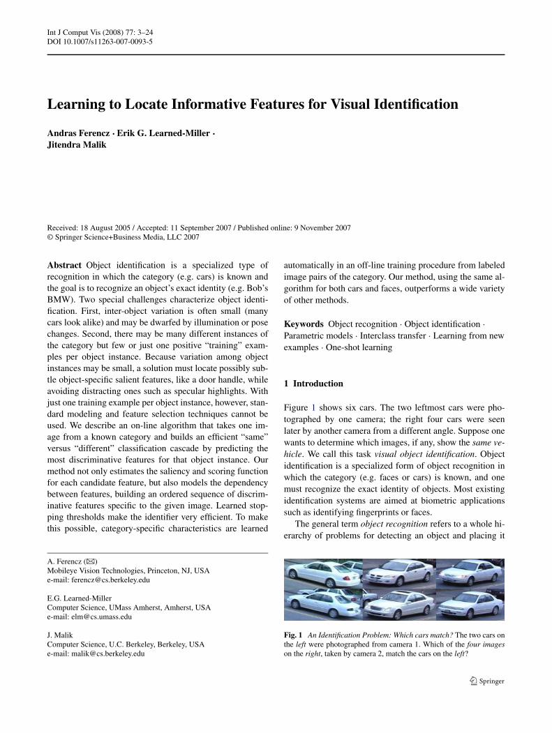
Figure 1 shows six cars. The two leftmost cars were pho-tographed by one camera; the right four cars were seenlater by another camera from a different angle. Suppose onewants to determine which images, if any, show the same ve-hicle. We call this task visual object identification. Objectidentification is a specialized form of object recognition inwhich the category (e.g. faces or cars) is known, and onemust recognize the exact identity of objects. Most existingidentification systems are aimed at biometric applicationssuch as identifying fingerprints or faces.

The general term object recognition refers to a whole hi-erarchy of problems for detecting an object and placing it

Fig. 1 An Identification Problem: Which cars match? The two cars onthe left were photographed from camera 1. Which of the four imageson the right, taken by camera 2, match the cars on the left?

4 Int J Comput Vis (2008) 77: 3–24

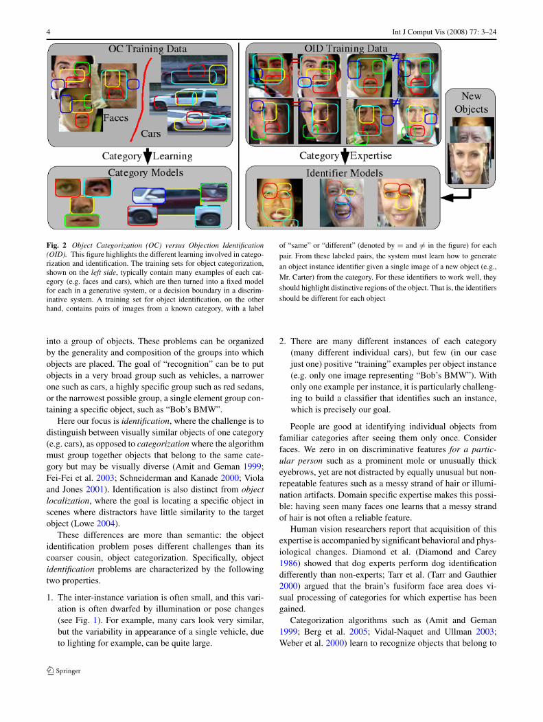
Fig. 2 Object Categorization (OC) versus Objection Identification(OID). This figure highlights the different learning involved in catego-rization and identification. The training sets for object categorization,shown on the left side, typically contain many examples of each cat-egory (e.g. faces and cars), which are then turned into a fixed modelfor each in a generative system, or a decision boundary in a discrim-inative system. A training set for object identification, on the otherhand, contains pairs of images from a known category, with a label

of “same” or “different” (denoted by = and �= in the figure) for eachpair. From these labeled pairs, the system must learn how to generatean object instance identifier given a single image of a new object (e.g.,Mr. Carter) from the category. For these identifiers to work well, theyshould highlight distinctive regions of the object. That is, the identifiersshould be different for each object

into a group of objects. These problems can be organizedby the generality and composition of the groups into whichobjects are placed. The goal of “recognition” can be to putobjects in a very broad group such as vehicles, a narrowerone such as cars, a highly specific group such as red sedans,or the narrowest possible group, a single element group con-taining a specific object, such as “Bob’s BMW”.

Here our focus is identification, where the challenge is todistinguish between visually similar objects of one category(e.g. cars), as opposed to categorization where the algorithmmust group together objects that belong to the same cate-gory but may be visually diverse (Amit and Geman 1999;Fei-Fei et al. 2003; Schneiderman and Kanade 2000; Violaand Jones 2001). Identification is also distinct from objectlocalization, where the goal is locating a specific object inscenes where distractors have little similarity to the targetobject (Lowe 2004).

These differences are more than semantic: the objectidentification problem poses different challenges than itscoarser cousin, object categorization. Specifically, objectidentification problems are characterized by the followingtwo properties.

1. The inter-instance variation is often small, and this vari-ation is often dwarfed by illumination or pose changes(see Fig. 1). For example, many cars look very similar,but the variability in appearance of a single vehicle, dueto lighting for example, can be quite large.

2. There are many different instances of each category(many different individual cars), but few (in our casejust one) positive “training” examples per object instance(e.g. only one image representing “Bob’s BMW”). Withonly one example per instance, it is particularly challeng-ing to build a classifier that identifies such an instance,which is precisely our goal.

People are good at identifying individual objects fromfamiliar categories after seeing them only once. Considerfaces. We zero in on discriminative features for a partic-ular person such as a prominent mole or unusually thickeyebrows, yet are not distracted by equally unusual but non-repeatable features such as a messy strand of hair or illumi-nation artifacts. Domain specific expertise makes this possi-ble: having seen many faces one learns that a messy strandof hair is not often a reliable feature.

Human vision researchers report that acquisition of thisexpertise is accompanied by significant behavioral and phys-iological changes. Diamond et al. (Diamond and Carey1986) showed that dog experts perform dog identificationdifferently than non-experts; Tarr et al. (Tarr and Gauthier2000) argued that the brain’s fusiform face area does vi-sual processing of categories for which expertise has beengained.

Categorization algorithms such as (Amit and Geman1999; Berg et al. 2005; Vidal-Naquet and Ullman 2003;Weber et al. 2000) learn to recognize objects that belong to

Int J Comput Vis (2008) 77: 3–24 5

a category. Here, we are attempting to go one step beyondthis by becoming category experts, where instead of havinga fixed set of features that we look for to recognize new ob-ject instances, we are able to predict the features of the newobject that will be the most informative for distinguishing itfrom other objects of the same category. Figure 2 highlightsthis difference. Note that categorization is a prerequisite foridentification, because identification systems such as oursassume that the given objects are from the known category.

1.1 The Three Steps of Object Identification

To clearly characterize the differences between object cate-gorization and the main subject of this paper, object identifi-cation, we enumerate the key steps in each process. We com-pare our object identification method with the traditional su-pervised learning paradigm of object categorization.

1.1.1 Object Categorization

In the simplest supervised learning framework for objectcategorization, the learner is supplied with two sets of ex-amples: a set of positive examples that are in a category (likecars), and a set of negative examples that are not in the cat-egory. The standard procedure of categorization consists oftwo steps:

1. Training a classifier using examples labeled positive (inthe category) and negative (not in the category), and

2. Applying the classifier to a new example to label it aspositive or negative.

Theoretically, we could use the same scheme to do objectidentification. To recognize a particular individual, such asGeorge Bush, we could collect sets of positive and nega-tive examples, and use the traditional supervised learningmethod just described. As remarked previously, however,we would like to be able to identify an individual after see-ing only a single picture. Traditional categorization schemeswork very poorly when trained on only a single example. Toaddress this lack of “training” data, we develop an entirelynew scheme, based upon developing category expertise, andusing this expertise to develop a customized identifier foreach instance we wish to recognize.

1.1.2 Object Identification

In our new scheme, there are three steps rather than two. Inthe first step, performed off-line on training data, we developexpertise about the general category, such as faces. This isdone by comparing the corresponding patches of many ex-ample pairs, some that match and some that do not. The goalis to analyze patch differences for each type of image pair,matching and non-matching, to understand under what con-ditions, we expect patches to be similar or different.

The expectation of the degree of differences between cor-responding patches can depend upon many factors. Patchesthat are not covering the face should not match well evenif it is the same person, while patches from the eye area arelikely to match well if the images are of the same person, butnot for different people. On the other hand, patches from thecheek area may match well even when the images are not ofthe same person (due to the frequent lack of texture in thisregion). Finally, forehead images from the same person arelikely to match if there is no hair in the patch, but may notmatch well if there is hair, since hair is highly variable fromappearance to appearance. These intuitions translate into a“scoring function” that relates the appearance similarity ofindividual matched patches to an indication of equivalenceof the whole face.

In addition to modeling the appearance differencesamong patches conditioned on the type, location and appear-ance of the patches, we can also estimate the expected util-ity or discriminativeness of a single patch from this analy-sis. We rate the discriminativeness of a patch by consideringwhether the expected differences with a corresponding patchdepend heavily on whether the faces match or not. For ex-ample, since a pair of corresponding patches which do notcover a portion of the face are expected to have large differ-ences, irrespective of whether the faces match or not, suchpatches have low expected utility. On the other hand, patchesnear the eye region are expected to have small differenceswhen the faces match, but to have larger differences whenthe faces do not match, and hence are expected to have highutility. In summary, the first step of our procedure producesmodels of patch differences conditioned on a variety of vari-ables, and also allows us to assess the expected utility of agiven patch based upon the patch difference models.

In the second step, which occurs at “test time”, we usethis expertise to build an identifier (more specifically anidentification cascade) for an object instance given a singleimage of that object. For each patch in the given image, weselect a specific model of patch appearance differences fromthe global model of patch appearance differences defined inthe first step. Then, using these models of patch appearancedifferences for each patch, we analyze the discriminative-ness of each patch in the given image. Finally, we sort thepatches in order from most discriminative to least discrimi-native.

In the third step, we use the object specific identifier todecide whether other instances of the category are the sameas or different than the given instance. This is done by com-paring patches in the given image (the “model” image) tocorresponding patches in another image (a “database” or“test” image). The most discriminative patches (as orderedin the second step) are used first and followed, if still neces-sary, by those with less discriminative power.

In summary, we define the steps in object identificationas:

6 Int J Comput Vis (2008) 77: 3–24

1. Learning a global model of patch1 differences, and asa result, a model of patch discriminativeness,

2. Building an identification cascade for a specific ob-ject instance by selecting, from the global model, object-specific models of patch differences and sorting thepatches by discriminativeness, and

3. Applying the identification cascade to novel images toassess whether they are the same or different as the spe-cific object instance for which the cascade was built.

We note that the last step of object categorization andthe last step of our scheme for object identification are es-sentially the same. In the case of object categorization, weapply a categorizer to a new example to decide whether itrepresents a category of interest. In the case of object iden-tification, we apply an identifier to a new example to decidewhether it is the same object as the single given training ex-ample. Other than this last step, however, the two paradigmsare quite different.

While the traditional object categorization scheme en-codes information at only one level, the level of the objectcategory, the identification scheme encodes two types of in-formation. In the first step of object identification, we en-code information about the entire category. In the secondstage, we encode information about the specific object in-stance. It is the use of the category expertise learned inthe first step that enables us to build effective identifiersfrom just a single example of each object. Without the cat-egory level information, it would be impossible to tell howto weight various areas of the image from only a single ex-ample. Our key contribution is a novel method for encodingthe category information so that we can use it effectively todefine an identifier for a new object instance.

1.1.3 Hyper-features

As stated above, in step 1 of our object identificationprocess, we analyze corresponding patches in image pairs todevelop a global model of which types of patches are likelyto be useful and which are not, and for the patches that areuseful, to know how to score a correspondence. This modelneeds to generalize to whole space of possible patches sothat at test time we can predict the utility and build a scoringfunction for patches of new instances (e.g. new car models)that were not in the training set.

Given that we register objects before analyzing patches,it should not be surprising that patches from certain parts

1To simplify the exposition, we have described the process of learningcategory expertise in terms of learning a model of patch discriminative-ness, which is how the identifiers in this paper were built. However, itis straightforward to generalize this general scheme to encode categoryinformation in a way other than modeling patches—for example, bymodeling the distributions of colors in images.

of the image tend to be more informative than patches fromother parts of an image. For example, when faces are reg-istered to a canonical position by centering them in an im-age, the patches in the upper corners of the image tend torepresent background, and hence are unlikely to be usefulfor discrimination. Hence, the spatial location of a patch isuseful in predicting its future utility in discrimination, evenwhen we do not yet know the patch we might be comparingit against. This type of “conditioning” on spatial location topredict utility is common in computer vision.

In this paper, however, we introduce a novel method forpredicting the utility of image patches that goes beyondmerely conditioning on spatial location. In particular, wealso use appearance features of a patch to predict its utility.For example, a patch of someone’s cheek that is uniformlycolored is not likely to be very discriminative since there isa strong possibility the corresponding patch on another dif-ferent person’s face would be indistinguishable, causing thispatch to be of no value in discrimination. However, if thepatch on someone’s cheek shows a distinctive mole or scar,its predicted utility dramatically increases, since this featurewould be unlikely to be repeated unless we are comparingagainst the same person.

Conditioning on visual features to predict utility, in ad-dition to spatial location, gives our patch discriminativenessmodels much more power. We call these features on whichwe condition hyper-features, and their use to model imagedifferences is the main contribution of this work.

The remainder of the paper is organized as follows. Sec-tion 2 discusses previous work in a number of areas. Sec-tion 3 summarizes the three stages of our algorithm: learningclass expertise in training, building an identification cascadefor a specific example, and running the identifier. Section 4details our model for estimating “same” and “different” dis-tributions for a patch. Section 5 describes our patch depen-dency model that allows us to generate a sequence of infor-mative patches. From this sequence, we build the cascade inSect. 6 by finding stopping thresholds for making “same” or“different” decisions. Section 7 details our experiments onmultiple car and face data sets.

2 Comparison to Previous Work

In this section, we highlight relevant previous papers anddescribe how our method differs or improves on them.

2.1 Part-Based Recognition

Breaking an image into local subparts, where each part isencoded and matched separately, is a popular techniquefor object recognition (both categorization and identifica-tion) (Berg et al. 2005; Bernstein and Amit 2005; Dork and

Int J Comput Vis (2008) 77: 3–24 7

Schmid 2005; Heisele et al. 2000; Kadir and Brady 2001;Lowe 2004; Mori et al. 2001; Vidal-Naquet and Ullman2003; Viola and Jones 2001; Weber et al. 2000; Wiskottet al. 1997). This strategy helps to mitigate the effects ofdistortion due to pose variation, as local regions are morelikely than the whole object to be related by simple trans-formations. It also contains the disturbance due to occlusionand localized illumination effects such as specularities. Fi-nally, it separates modeling of appearance and position. Thekey idea is that the parts, which are allowed to move rela-tive to one other, can be treated as semi-independent assess-ments for the recognition task. The classifier then combinesthis evidence, optionally using the positional configurationof the detected parts as an additional cue, to determine thepresence or absence of the object.

Due to the constraints of object identification describedin the introduction, our system differs from previous work ina fundamental way. In the above systems, a model consist-ing of informative parts and (optionally) their relationshipsis learned from a set of object and background examples.This “feature selection” step is fundamental to these meth-ods and is possible because statistics such as the frequencyof appearance of a particular feature (e.g., a quantized SIFTvector) can be directly computed for the positive and neg-ative examples of a class. Thus these systems rely on un-derlying feature selection (and weighting) techniques suchas Conditional Mutual Information (Fleuret 2004) or Ad-aBoost (Freund and Schapire 1996). In our setting this is notpossible because only one example of a particular categoryinstance (which plays the role of a “class” in our setting)will be presented, which is not enough to directly estimatethe discriminativeness of any feature. Our main contributionis overcoming this fundamental barrier by learning a modelfor the space of all possible features tuned to a particularcategory (e.g., cars) that then allows us to pick the discrim-inative features for the given category instance (e.g., Bob’BMW).

A minor additional difference compared to many of theabove techniques is the choice of part representation. Pop-ular encodings such as SIFT (Lowe 2004), which are de-signed to be invariant to significant distortions, are toocoarse for our needs—they often destroy the very infor-mation that distinguishes one instance from another. Thuswe use a more dense representation of multiple filter chan-nels. However, we stress that this is not fundamental to ourmethod, and any part encoding and comparison metric couldbe used within our learning framework.

2.2 Interclass Transfer

Because of the lack of training data for a particular in-stance, the general framework of most object recognitionsystems, that of selecting informative features using a set of

object/non-object examples, is impossible to directly applyto our setting. In view of this difficulty, given a new cate-gory instance (e.g., Bob’s BMW), how can we pick goodfeatures, and how can we combine them to build an objectinstance identifier?

One possible solution is to try to pick universally goodfeatures, such as corners (Kadir and Brady 2001; Lowe2004), for detecting salient points. However, such featuresare not category specific: we expect to use different kindsof image features when distinguishing Bob’s car from othercars versus when we are distinguishing Bob’s dog from an-other dog.

Another possibility is to build generative models for eachclass including such characteristics as the typical illumina-tions, likely deformations, and variation in viewing direc-tion. With a precise enough model, an algorithm should beable to find good features for discriminating instances of thecategory from each other (Blanz et al. 2002). Alternatively,good features could be explicitly coded into the algorithm(Wiskott et al. 1997). However, this tends to be complicatedand time consuming, and must be done individually for aparticular category (see Sect. 2.4 below for examples). Ad-ditionally, one might hope that given a good statistical modeland a large training data set, an algorithm would actually bebetter at finding informative features.

A better option is to attempt to transfer models from pre-vious classification tasks of the same category (interclasstransfer). Thrun (1996) introduces such an interclass trans-fer (also referred to as lifelong learning or learning-to-learn)framework, in which a series of similar learning tasks arepresented, where each subsequent task uses the model thatwas built for the previous tasks. More recently (Miller et al.2000), distributions over parameters of a similarity transfor-mation learned from one group of classes (letters) are usedto model other classes (digits) for which only a single ex-ample is provided. In other work (Fei-Fei et al. 2003), priorsfor a fixed-degree constellation model are learned from oneset of classes to train a detector for a new class given only asmall number of positive examples of that class.

In all of these works, the set of hidden variables (the fea-tures used by Thrun 1996, the transformations in Miller et al.2000, or the parameters of the constellation model in Fei-Feiet al. 2003) are predefined and the generalization from othercategories can be thought of as learning priors for these fixedsets of variables. In contrast, we wish to learn how to iden-tify any number of good features that are present in the sin-gle “training” example for an object instance that can then beassembled into a binary classification cascade. This forcesus to learn a model for the space of all possible features (inour case, image patches).

8 Int J Comput Vis (2008) 77: 3–24

2.3 Pairwise Constraints

The machine learning literature provides a different perspec-tive on our interclass transfer problem. Our problem can bethought of as a standard learning task where the input is apair of images, and the output is a “same” vs. “different”label. The task is then to learn a “distance metric” betweenimages, specifically by choosing and weighting relevant fea-tures.

Recent work on equivalence constraints such as RelevantComponent Analysis (Shental et al. 2002) and others (Shen-tal et al. 2003; Xing et al. 2002) show how to optimize adistance metric over the input space of features that mapsthe “same” pairs close to one another while keeping “differ-ent” ones apart. In our setting, the transformations that wewould be interested in are subset selection and weighting(although our technique does more then weight each fea-ture). These methods, however, assume that each example isdescribed by the same predefined set of features, and that thecomparison function is a specific distance metric over thesefeatures (e.g., Euclidean).

In our case, the “features” we are trying to use are sub-patches of one image, compared to the best correspondinglocation in the other image. Thus our feature space is veryhigh dimensional, and the comparison method is not a sim-ple distance metric (notice, for example, that it is not sym-metric due to the local search of best corresponding patch).Even if this space of features were discretized, it would beimpossible to enumerate all possible such features, and mostwould never appear within the training set. These differ-ences make our algorithm very different from other pairwiseconstraint techniques.

A core observation of this paper is that it is not necessaryto enumerate all possible features. Instead, we can model thespace of the features in a way that allows us to estimate theinformativeness of novel features that the algorithm was notdirectly trained on (informative means that when this patchis compared to the best corresponding patch in a test image,the appearance similarity gives us information about the testimage being the “same” or “different”). Thus we model thisspace of features (in our case, each feature is defined by thesize, position and appearance of the image patch) using asmooth function (actually a pair of them, one based on thematching to the “same” cars and one based on “different”pairs). Then, given a new instance, the algorithm can selectthe most informative patches among the ones that are actu-ally present in that image. Furthermore, our pair of functionsgives us a way to convert the patch matching distance to ascore for each selected patch (this is similar to but has moredegrees of freedom then a linear feature weight).

Here our features are image patches. We note, however,that our technique could be used in any setting where RCAis used when the features can be embedded into a continu-ous space. This has the potential advantage of exploiting the

relationship between the features that the above techniqueshave no access to.

2.4 Face Identification

Our goal in this work is to develop an identification sys-tem that is not designed for any particular category, but in-stead automatically learns category-specific characteristics.Nonetheless, it is useful to consider previous identificationsystems that were designed with a particular category inmind. Here we highlight a few face identification systemsthat are representative and relevant for our work. For an ex-tensive survey of the field, we refer the reader to Zhao et al.(2003).

Techniques such as Eigenfaces (Turk and Pentland 1991)(PCA), Fisherfaces (Belhumeur et al. 1997) (LDA), andBayesian face recognition (Moghaddam et al. 2000), likeour method, start with a general face modeling step, andlater make a same/difference determination for a new face.Bayesian face recognition, which won the 1996 FERETcompetition, explicitly uses “same” and “different” equiv-alence constraints similar to the techniques described inSect. 2.3. These are all “holistic” techniques in that they usethe whole face region as raw input to the recognition system.Specifically, they take registered and intensity normalizedfaces (or labeled collections of images in the case of LDAand Bayesian techniques) and find a lower dimensional sub-space that, it is hoped, is more conducive to identification.This is analogous to Step 1 in our procedure. To build a clas-sifier, the model image is projected into this subspace, andthe classifier compares the model and test images within thissubspace.

More complex, feature-based methods typically use moreface-specific models and hand labeled data. Two techniquesin this category that have had a significant impact are elas-tic bunch graph matching (Wiskott et al. 1997), where handselected fiducial points are matched within a graph that de-fines their relative positions, and the method of Blanz andVetter (Blanz et al. 2002), which maps images onto a 3Dmorphable face model.

We now turn to a more detailed description of ourmethod.

3 Algorithm Overview

In this section, we outline the basic components of our sys-tem. After discussing initial preprocessing and alignment,we describe the three stages of our algorithm: global mod-eling of patch differences, building an identification cascadefrom one example, and application of the identification cas-cade. For clarity of exposition, we describe these stages inreverse order.

Int J Comput Vis (2008) 77: 3–24 9

3.1 Preprocessing: Detection and Alignment

Our algorithm, as most identification systems, assumes thatall images are known to contain objects of the given category(e.g. cars or faces) and have been brought into rough cor-respondence. For our algorithm, an approximate alignmentis sufficient, because we search for matching patches in asmall neighborhood (in our data sets 10–20% of image size)around the expected location. No foreground-backgroundsegmentation is required, as the system learns which fea-tures within the images (both in terms of position and ap-pearance) are useful for identification—thus patches that areoff of the object are rejected by the learning algorithm. Thespecific detection and alignment methods used for our var-ious data sets are described in Sect. 7. For example, for theCars 2 data set, objects were aligned based only on the cen-troid of a simple background subtraction based blob detec-tor.

3.2 Applying the Object Instance Identifier

We now describe the object instance identifier, which is thefinal step in our three step identification system. We start byintroducing some notation.

We assume that at test time, we are given a single im-age of an object instance, known as the model image. Thegoal will be to compare it to a large set of database images,known as test images. For each pair of images (the modelimage and one of the test images) we wish to make a deter-mination about whether the images represent the same spe-cific object, or two different objects. The variable C willrepresent this match/mismatch variable, with C = 1 denot-ing that the two images are of the same object (i.e., theymatch) and C = 0 denoting that the two images are of dif-ferent objects (i.e., they do not match).

For the purposes of illustration, we will often presentpairs of images side by side, where the image on the leftwill be the model image and the image on the right will beone of the test images (Figs. 3, 4, 10, 14). Thus we use IL torefer to the model image and IR to refer to the current testimage. Thus, the identifier for a particular object instancedecides if a test image (or “right” image) IR is the same as(C = 1) or different than (C = 0) the model image (or “left”image) IL it was trained for.

3.2.1 Patches

Our strategy is to break up the whole image comparisonproblem into the comparison of patches (Vidal-Naquet andUllman 2003; Weber et al. 2000). The m (possibly overlap-ping) patches in the left image will be denoted FL

j , with1 ≤ j ≤ m. The corresponding patches in the right imageare denoted FR

j .

Although the exact choice of features, their encoding andthe comparison metric are not crucial to our technique, wewanted to use features that were general enough to use in awide variety of settings, but informative enough to capturethe relative locality of object markings as well as large andsmall details of objects.

For our experiments, our patch sizes ranges from 12×12pixels to the size of the full image, and are not constrained tobe square. To compute the patch features, we begin by com-puting a Gaussian pyramid for each image. For each patch,based on its size, the image pixels are extracted from a levelof the pyramid such that the number of pixels in the rep-resentation is approximately constant (for our experiments,all of our patches, except the smallest ones taken from thelowest level of the pyramid, contained between 500 and 750pixels). Then we encode the pixels by applying a first deriva-tive Gaussian odd-symmetric filter to the patch at four orien-tations (horizontal, vertical, and two diagonal), giving foursigned numbers per pixel. The patch FL

j is defined by itsappearance encoding, position (x, y) and size (w,h).

3.2.2 Matching

To compare a model patch FLj to an equally encoded area of

the right image FRj , we evaluate the normalized correlation

and compute

dj = 1 − CorrCoef(FLj ,FR

j ) (1)

between the arrays of orientation vectors. Thus dj is a patchappearance distance where 0 ≤ dj ≤ 2.

As the two images to be compared have been processedto be in rough alignment, we need only search a small areaof IR to find the best corresponding patch FR

j —i.e., the onethat minimizes dj . We will refer to such a matched left andright patch pair FL

j ,FRj , together with the derived distance

dj , as a bi-patch. This appearance distance dj is used asevidence for deciding if IL and IR are the same (C = 1) ordifferent (C = 0).

In choosing this representation and comparison function,we compared a number of commonly used encodings, in-cluding Lowe’s SIFT features (Lowe 2004) and shape con-texts (Belongie et al. 2001). However, we found that due tothe nature of the problem—where distinct objects can lookvery similar except for a few subtle differences—these tech-niques, which were developed to be insensitive to small dif-ferences, did not perform well. Specifically, using SIFT fea-tures as described in Lowe (2004) (without category specificlearning) resulted in false-positive error rates that were anorder of magnitude larger than our best results and a fac-tor of 2–3 worse than our baseline results (at the same re-call rate). Among dense patch features, we chose normalizedcorrelation of filter outputs after experiments comparing this

10 Int J Comput Vis (2008) 77: 3–24

distance function to L1 and L2 distances, and the encodingto raw pixels and edges as described elsewhere (Weber et al.2000).

3.2.3 Likelihood Ratio Score

We pose the task of deciding if a test image IR is the sameas a model image IL as a decision rule

R = P(C = 1|IL, IR)

P (C = 0|IL, IR)(2)

= P(IL, IR|C = 1)P (C = 1)

P (IL, IR|C = 0)P (C = 0)> λ (3)

where λ is chosen to balance the cost of the two types ofdecision errors. The prior probability of C is assumed tobe known.2 Specifically, for the remaining equations in thispaper, the priors are assumed to be equal, and hence aredropped from subsequent equations.

With our image decomposition into patches, the poste-riors from (2) will be approximated using the bi-patchesF1, . . . ,Fn as

P(C|IL, IR) ≈ P(C|F1, . . . ,Fm) (4)

∝ P(F1, . . . ,Fm|C). (5)

Furthermore, we will assume a naive Bayes model in which,conditioned on C, the bi-patches are assumed to be indepen-dent (see Sect. 5 for our efforts to ensure that the selectedpatches are, in fact, as independent as possible). That is,

R = P(IL, IR|C = 1)

P (IL, IR|C = 0)(6)

≈ P(F1, . . . ,Fm|C = 1)

P (F1, . . . ,Fm|C = 0)(7)

=m∏

j=1

P(Fj |C = 1)

P (Fj |C = 0). (8)

In practice, we compute the logarithm of this likelihood ra-tio, where each patch contributes an additive term. Modelingthe likelihoods P(Fj |C) in this ratio is the central focus ofthis paper.

In our current system, the only information from bi-patchFj that we use for scoring is the distance dj . Thus, to con-vert dj to a score, the object instance identifier must con-sist of probability distribution functions P(Dj |C = 1) andP(Dj |C = 0) for each patch in the model image. Thesefunctions encode our expectations about how well we ex-pect a patch in the test image to match a particular patch

2For our car tracking application (see Sect. 7.3), dynamic models oftraffic flow can supply the prior on P (C).

(j ) in the model image, depending upon whether or not theimages themselves represent the same object instance.

The object instance identifier computes the log likelihoodratio by evaluating these functions for each dj obtained bycomparing the model image patches to test image patches.(A comment on notation: dj refers to the specific measureddistance for a given model image patch and the correspond-ing test image patch, while Dj denotes the random vari-able from which dj is a sample.) After m patches have beenmatched, assuming independence, we score the match be-tween images IL and IR using the sum of log likelihoodratios of matched patches:

R =m∑

j=1

logP(Dj = dj |C = 1)

P (Dj = dj |C = 0). (9)

To compute this quantity, we must evaluate P(Dj =dj |C = 1) and P(Dj = dj |C = 0). In our system, both ofthese will take the form of gamma distributions �(dj ; θC=1

j )

and �(dj ; θC=0j ), where the parameters θC=1

j and θC=0j for

each patch and matching condition are defined as part of theobject instance identifier. How we set these parameters usinga single image is discussed in Sect. 3.3.

3.2.4 Making a Decision

The object instance identifier described above compared afixed number of patches (m), computed the score R by (9),and compared it to a threshold λ. R > λ means that IL andIR are declared to be the same. Otherwise they are declareddifferent. In Sect. 6, we define a more efficient object in-stance identifier by building a cascade from the sequence ofpatches. This is done by applying early termination thresh-olds λC=1

k (for early match detection) or λC=0k (for early

mismatch detection) after the first k patches have been com-pared. These thresholds may allow the object instance iden-tifier to stop and declare a result after comparing only k

patches.

3.2.5 Summary of the Object Instance Identifier

To summarize, the object instance identifier is defined by

1. a sequence of patches of varying sizes FLj taken from the

model image IL,2. for each patch FL

j , a pair of parameters θC=1j and

θC=0j that define the distributions P(Dj |C = 1) and

P(Dj |C = 0), and3. optionally, a set of thresholds λC=1

k and λC=0k applied

after matching the kth patch.

For an example, refer to Fig. 3.

Int J Comput Vis (2008) 77: 3–24 11

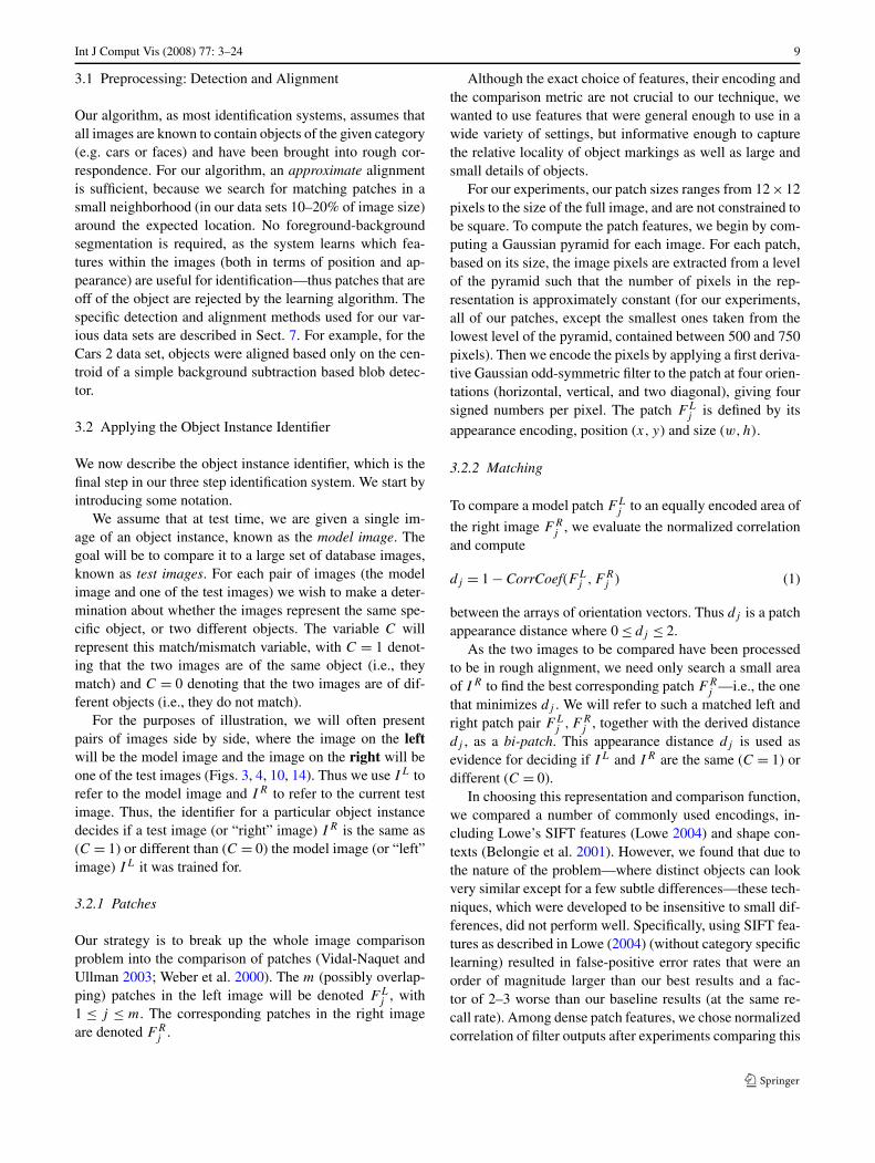
Fig. 3 (Color online) The Object Instance Identifier. On the left, amodel image IL is shown with an identifier composed of three patches(these would not be the actual top three patches selected by our sys-tem. To build the identifier, the three patches were analyzed to selectthree “same” and “different” distributions from the global model ofpatch differences. The red curve in each plot, which for good featuresis the left peak, represents the “same” distribution, while the other bluecurve represents the “different” distribution. Our patch encoding usingoriented filter channels is shown for patch 2. The object instance identi-fier matches the patches to the test images, computes the log likelihoodratio score for each using the estimated distributions, and makes a same

versus different decision based on the sum R. (The top image is thecorrect match.) Looking at the images, compare the informativeness ofpatches 1 and 3: matching patch 1 should be very informative, sincethe true matching patch (top) is much more similar then the matchingpatch in the other “different” image (bottom); matching patch 3 shouldbe much less informative, as both matching test image patches lookhighly dissimilar to the corresponding model patch. The superiority ofpatch 1 was inferred correctly by our system based on the position andappearance of these patches in the model image only, as shown by themutual informations I (Dj |C) for each patch, which are functions onlyof the model image patches

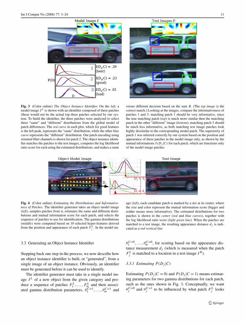
Fig. 4 (Color online) Estimating the Distributions and Informative-ness of Patches. The identifier generator takes an object model image(left), samples patches from it, estimates the same and different distri-butions and mutual information score for each patch, and selects thesequence of patches to use for identification. The gamma distributions(middle) were computed based on 10 selected hyper-features derivedfrom the position and appearance of each patch FL

j . In the model im-

age (left), each candidate patch is marked by a dot at its center, wherethe size and color represent the mutual information score (bigger andredder means more informative). The estimated distributions for twopatches is shown in the center (red and blue curves), together withthe log likelihood ratio score (light green line). When the patches arematched to a test image, the resulting appearance distance dj is indi-cated as a red vertical line

3.3 Generating an Object Instance Identifier

Stepping back one step in the process, we now describe howan object instance identifier is built, or “generated”, from asingle image of an object instance. Obviously, an identifiermust be generated before it can be used to identify.

The identifier generator must take in a single model im-age IL of a new object from the given category and pro-duce a sequence of patches FL

1 , . . . ,FLm and their associ-

ated gamma distribution parameters, θC=11 , . . . , θC=1

m and

θC=01 , . . . , θC=0

m , for scoring based on the appearance dis-tance measurement dj (which is measured when the patchFL

j is matched to a location in a test image IR).

3.3.1 Estimating P(Dj |C)

Estimating P(Dj |C = 0) and P(Dj |C = 1) means estimat-ing parameters for two gamma distributions for each patch,such as the ones shown in Fig. 3. Conceptually, we wantθC=0j and θC=1

j to be influenced by what patch FLj looks

12 Int J Comput Vis (2008) 77: 3–24

like and where it is on the object. That is, we want a pairof functions QC=1 and QC=0 that map the position and ap-pearance of the patch FL

j to the parameters of the gamma

distribution θC=1j and θC=0

j :

QC=1 : FLj �→ θC=1

j ,

QC=0 : FLj �→ θC=0

j .

These functions are estimated in the initial training phase(Step 1), and how they are estimated is discussed at lengthbelow.

3.3.2 Estimating Saliency

If we define the saliency of a patch as the amount of infor-mation about the decision likely to be gained if the patchwere to be matched, then it is straightforward to estimatesaliency given P(Dj |C = 1) and P(Dj |C = 0). Intuitively,if P(Dj |C = 1) and P(Dj |C = 0) are similar distributions,we do not expect much useful information from a valueof dj . On the other hand, if the distributions are very dif-ferent, then dj can potentially tell us a great deal about ourdecision. Formally, this can be measured as the mutual in-formation between the decision variable C and the randomvariable Dj :

I (Dj ;C) = H(Dj ) − H(Dj |C).

Here H() is Shannon entropy. Notice that this measure canbe computed just from the estimated distributions of Dj ,which, in turn, were estimated from the position and appear-ance of the model patch FL

j , before the patch has ever beenmatched.

3.3.3 Finding Good Patches

The above mutual information formula allows us to esti-mate the saliency of any patch. Thus defining a sequenceof patches to examine in order, from among all candidatepatches, seems straightforward:

1. for each candidate patch(a) estimate the distributions P(Dj |C) from FL

j using

the functions QC

(b) compute the mutual information I (Dj ;C)

2. choose the top m patches sorted by I (Dj ;C).

The problem with this procedure is that the patches are notindependent. Once we have matched a patch FL

j , the amountof additional information we are expected to derive frommatching a patch FL

i that overlaps FLj is likely to be less

than the mutual information I (Di;C) would suggest. Wediscuss a solution to this problem in Sect. 5.

However, assuming that this dependency problem can besolved, and given the functions QC , we have a complete al-gorithm for generating an object instance identifier from asingle image.

3.4 Off-line Training

Finally, we complete our reverse-order discussion by de-scribing the first major step of our system, learning abouta given category (e.g., cars) from training data. This proce-dure is done only once, and happens prior to testing.

The off-line training procedure defines the two functionsQC=1 and QC=0 that estimate the parameters of the gammadistributions P(Dj |C = 1) and P(Dj |C = 0) from the po-sition and appearance of a model image patch FL

j . Addi-tionally, it builds a dependency model among patches anddefines the early termination cascade thresholds λC=1

k andλC=0

k .This off-line training starts with a large collection of im-

age pairs from the category (see Sect. 7 for details aboutour data sets), where each left-right image pair is labeled as“same” or “different”. A large number of patches FL

j aresampled from the left images. Each patch is compared to itscorresponding patch in the right image. The correspondenceis defined by finding the best matching patch over a smallsearch area around the same location in the second image.Once the corresponding patch is found in the right image,the resulting value of dj is recorded and associated with theoriginal patch from the left image.

The functions QC=0 and QC=1 will ultimately be poly-nomial functions of the hyper-features, that is, the locationand appearance features of each patch. These polynomialsare estimated in a maximum likelihood framework using ageneralized linear model. In short, the functions QC=1 andQC=0 are optimized to produce gamma distributions whichmaximize the likelihoods P(dj |C) of the patch differencedata from training. The details of this estimation are dis-cussed in the following section.

4 Hyper-features and Generalized Linear Models

In this section, we describe in detail how to estimate, fromtraining data, the functions QC=0 and QC=1 that map theposition and appearance of a model image patch FL

j to the

parameters θCj of the gamma distributions for P(Dj |C).

We want to differentiate patches by producing distrib-utions P(Dj |C = 1) and P(Dj |C = 0) tuned for patchFL

j . When a training set of “same” (C = 1) and “differ-ent” (C = 0) images are available for a specific model im-age, estimating these distributions directly for each patchis straightforward. But how can we estimate the distribu-tion P(Dj |FL

j ,C = 1), where FLj is a patch from a new

Int J Comput Vis (2008) 77: 3–24 13

Fig. 5 Identification with Patches. The bottom curve shows the pre-cision vs. recall for non-patch based direct comparison of rectifiedimages (the most accurate technique we found was to match a fixedsubrectange of the image by searching for the best normalized correla-tion of the 4 filter channels). The other curves show the performanceof our algorithm on the Cars 1 data set, using all fixed sized patches(25 × 25 pixels) sampled from a grid such that each patch overlaps itsneighbors by 50%. Notice that all three patch based models outper-form the direct method. The three top curves show results for variousmodels of dj : (1) no dependence on patch characteristics (Baseline),

(2) using hyper-features in discrete bins Sect. 4.1 (Discrete), and (3)using a generalized linear model with hyper-feature selection fromSects. 4.2 and 4.3 (Continuous). The linear model significantly outper-forms all of others. Compared to the baseline patch method it reducesthe error in precision by close to 50% for most values of recall be-low 90% showing that conditioning the distributions on hyper-featuresboosts performance. Note: this figure differs from results presentedlater in that no patch selection was performed

model image, when we only have that single positive ex-ample of FL

j ? The intuitive answer: by finding analogouspatches in the training set of labeled (same/different) imagepairs. However, since the space of all possible patches3 isvery large, the chance of having seen a patch very similar toFL

j in the training set is small. In the next two subsectionswe present two approaches both of which rely on project-ing FL

j into a much lower dimensional space by extractingmeaningful features from its position and appearance, i.e.,the hyper-features.

4.1 Discrete Hyper-features

First we explore a binning approach, where we place hyper-features into a number of pre-specified axis-aligned bins.For example we might break the x-coordinate of the po-sition into four bins, the y-coordinate into three bins, andan appearance feature of the patch, such as contrast, intotwo bins. We would then label each patch with its positionin this 4-by-3-by-2 histogram. For each bin, we estimateP(Dj |FL

j ,C = 1) and P(Dj |FLj ,C = 0) by computing the

parameters (θCj ) of the gamma distributions from all of the

bi-patches Fj whose left patch FLj falls into that bin. More

3For a 25 × 25 patch, appearance plus position (including size) is apoint in �25×25+4.

precisely, we use bi-patches from the “same” image pairs toestimate θC=1

j and the “different” pairs to find θC=0j .4

Figure 5 compares the performance of various models onthe Cars 1 data set, which is described in Sect. 7.1. Here, forsimplicity of comparison, we use no patch selection (105patches are sampled at fixed, equally spaced locations) andpatch sizes are fixed to 25 × 25. The two bottom curves arebaseline experiments. The direct image comparison methodcompares the center part of the images using normalizedcorrelation on a combination of intensity and filter channelsand attempts to overcome slight misalignment. The patch-based baseline assumes a global distribution for Dj that isthe same for all patches.

The cyan “Discrete” curve in Fig. 5 shows the perfor-mance improvement from conditioning on discrete hyper-features.

4.2 Continuous Hyper-features

When too many hyper-feature bins are introduced, the per-formance of the discrete model degrades. The problem isthat the amount of data needed to populate the histograms

4Using the same binning of hyper-features, but modeling the resultingconditional distributions as normalized histograms, rather than gammadistributions, produces very similar results when enough data is avail-able in each bin.

14 Int J Comput Vis (2008) 77: 3–24

Fig. 6 (Color online) Fitting a generalized linear model to the gammadistribution. We demonstrate our approach by fitting a gamma dis-tribution, through the latent variables θ = (μ,σ ), to the y positionof the patches (in practice, we use the parameterization θ = (μ,γ )).Here we allowed μ and σ to be a 3rd degree polynomial function of y(i.e. Z = [y3,y2,y,1]T). Each row of the images labeled (a) displaysthe empirical density of d conditioned on the y position of the leftpatch (FL) for all bi-patches sampled from the training data (darkermeans higher density). There are two of these: one for bi-patches takenfrom matching vehicles (the pairs labeled “same”); the other from mis-matched data (“different” pairs). Row (b) shows the ordinary linearmodel fit, where the curve represents the mean. The outer curves in

(c) show the ±σ (one standard deviation) range fit by the GLM. Onthe bottom left, the centers of patches from a model object are labeledwith a dot whose size and color corresponds to the mutual informationscore I (D;C). For two selected rows, each representing a particular y

position, the empirical distributions are displayed as a histogram. Thegamma distributions as fit by the GLM are superimposed on the his-tograms. Notice that this model has learned that the top portion of thevehicles in the training set is not very informative, as the two distribu-tions (the red and blue lines in the top histogram plot) are very similar.That is, Dj will have low mutual information with C. In contrast, thebottom area is much more informative

grows exponentially with the number of dimensions. In or-der to add additional appearance-based hyper-features, suchas mean intensity, oriented edge energy, etc., we moved to apolynomial model to describe how hyper-features influencethe choice of gamma distribution parameters.

Specifically, as before, we model the distributions P(Dj |FL

j ,C = 1) and P(Dj |FLj ,C = 0) as gamma distributions

�(θC) parameterized by the mean and shape parameter θ ={μ,γ }. See the left side of Fig. 6 for examples of the gammaapproximations to the empirical distributions.

The smooth variation of θ with respect to the hyper-features can be modeled using a generalized linear model(GLM). Ordinary (least-squares) linear models assume thatthe data for each conditional distribution is normally dis-tributed with constant variance. GLMs are extensions to or-dinary linear models that can fit data which is not normally

distributed and where the dispersion parameter also dependson the covariates. See McCullagh and Nelder (1989) formore information on GLMs.

Our goal is to fit gamma distributions to P(Dj |FLj ,C =

1) and P(Dj |FLj ,C = 0) for various patches by maximiz-

ing the probability density of data under gamma distrib-utions whose parameters are simple polynomial functionsof the hyper-features. Consider a set X1, . . . ,Xk of hyper-features such as position, contrast, and brightness of a patch.Let Z = [Z1, . . . ,Zl]T be a vector of l pre-chosen monomi-als of those hyper-features, like squares, cubes, cross terms,or simply copies of the variables themselves. Then each bi-patch distance distribution has the form

P(d|X1,X2, . . . ,Xk,C) = �(d; αμ

C · Z, αγ

C · Z), (10)

Int J Comput Vis (2008) 77: 3–24 15

where the second and third arguments to �() are mean andshape parameters. Note that both the mean and shape pa-rameters are linear functions of the hyper-feature monomi-als Z, which is what makes this model a generalized linearmodel.

For our GLM, we use the identity link function5 for bothμ and γ . While the identity is not the canonical link func-tion for μ, its advantage is that our ML optimization canbe initialized by solving an ordinary least squares prob-lem. We experimentally compared it to the canonical inverselink (μ = (α

μC · Z)−1), but observed no noticeable change

in performance on our data set. Each α (there are four ofthese: α

μC=0, α

γ

C=0, αμC=1, α

γ

C=1) is a vector of parameters oflength l that weights each hyper-feature monomial Zi . Theα’s are adapted to maximize the joint data likelihood overall patches for C = 1 (using patches from the “same” im-age pairs) and for C = 0 (from the “different” image pairs)within the training set. These ideas are illustrated in detailin Fig. 6, where, for demonstration purposes, we let our co-variates Z = [y3,y2,y,1]T be a polynomial function of they position.

4.3 Automatic Selection of Hyper-features

While it is certainly possible to select the basic hyper-features X and their monomials Z manually, we make ad-ditional improvements to our system by considering largerpotential sets of hyper-feature monomials and using featureselection techniques to select only those that are most useful.

Recall that in our GLM model we assumed a linear rela-tionship between Z and μ. By ignoring the dispersion para-meter, this allows us to use standard feature selection tech-niques, such as Least Angle Regression (LARS) (Efron etal. 2004), to choose a few (around 10) hyper-features from alarge set of candidates. In order to use LARS (or most otherfeature selection methods) “out of the box”, we use regres-sion based on an L2 loss function. While this is not opti-mal for non-normal data, from experiments we have verifiedthat it is a reasonable approximation for the feature selectionstep.

To use LARS for feature selection, we start with a largeset of candidate hyper-feature monomials: (a) the x and ypositions of FL, (b) the intensity and contrast within FL

and the average intensity of the entire object, (c) the averageenergy in each of the four oriented filter channels, and (d)derived quantities from the above such as square, cubic, andcross terms as well as meaningful derived quantities such asthe direction of the maximum edge energy. LARS is usedto selected a subset of these, which act as the final set ofhyper-features Z. Once Z is set, we proceed as in Sect. 4.2.

5“Link function” and “canonical link function” are terms related togeneralized linear models. The reader should refer to GLM referencesfor discussions of these terms (McCullagh and Nelder 1989).

Running an automatic feature selection technique on thislarge set of possible conditioning features gives us a princi-pled method of reducing the complexity of our model. Re-ducing the complexity is important not only to speed upcomputation, but also to mitigate the risk of over-fitting tothe training set. The top curve in Fig. 5 shows results whenZ includes the first 10 features found by LARS. Even withsuch a naive set of features to choose from, the performanceof the system improves significantly. We believe that furtherimprovement in our results is possible by designing moresophisticated hyper-features.

5 Modeling Pairwise Relationships between Patches

In Sects. 3 and 4, we described our method for scoring amodel image patch FL

j and its best match FRj by modeling

the distribution of their difference in appearance, dj , condi-tioned on the match variable C. Furthermore, in Sect. 3.3,we described how to infer the saliency of the patch FL

j formatching based on these distributions. As we noted in thatsection, this works for picking the first patch, but is not op-timal for picking subsequent patches. Once we have alreadymatched and recorded the score of the first patch, the amountof information gained from a nearby patch is likely to besmall, because their scores are likely to be correlated. In-tuitively, the next chosen patch would ideally be a highlysalient patch whose information about C is as independentas possible from the first patch. Similarly, the third patchshould consider both the first and the second patches.

Let FL(k) represent the kth patch picked for the cascade

and let FL(1...n) denote the first n of these patches. Assume we

have already picked patches FL(1...n)

and we wish to choose

the next one, FL(n+1), from the remaining set of FL

j ’s. Wewould like to pick the one that maximizes the informationgain or the conditional mutual information:

I (D(n+1);C|D(1...n)) = I (D(1...n+1);C) − I (D(1...n);C).

This quantity is difficult to estimate, due to the need tomodel the joint distribution of all D(1...n) patches. However,note that the information gain of a new feature is upperbounded by the information gain of that feature relative toany single feature that has already been chosen. That is,

I (D(n+1);C|D(1...n)) ≤ min1≤i≤n

I (D(n+1);C|D(i)). (11)

Thus, rather than maximizing the full information gain,Vidal-Naquet and Ullman (2003) (see Fleuret 2004 for acomparison to other feature selection techniques) proposedthe following heuristic that maximizes this upper bound onthe amount of “additional” information:

arg maxj

mini

I (Dj ;C|D(i)), (12)

16 Int J Comput Vis (2008) 77: 3–24

where i varies over the already chosen patches, and j variesover the remaining patches.

We use a related, but slightly different heuristic. WhenDj and D(i) are completely correlated (that is, D(i) predictsDj ) then I (Dj ;C|D(i)) = 0. However, even when Dj andD(i) are completely independent given C, I (Dj ;C|D(i))

does not equal I (Dj ;C). This somewhat counterintuitiveresult is due to the fact that there is only a total of 1 bit ofinformation in C, some of which has already been discov-ered by matching patch Fj . This property causes problemsfor the above pairwise approximation, as in some circum-stances it might lead to choosing a suboptimal next patchF(i). In particular, a patch that is highly correlated with anuninformative patch might win out against another patchthat is lightly correlated with a very informative one. Hence,in order to find the best next patch, we use a quantity re-lated to I (Dj ;C|D(i)), but one which varies between 0 andI (Dj ;C) depending only on the correlation:

arg maxj

mini

I (Dj ;C|D(i)) × I (Dj ;C)

I (D∗j ;C|D(i))

. (13)

Here D∗j is a random variable with the same marginal dis-

tribution as Dj but is independent of D(i) when conditionedon C. This formulation also turns out to be easier to approx-imate within our framework (see Sect. 5.3).

5.1 Dependency Model

To compute (13), we need to estimate conditional mutualinformations of the form

I (Dj ;C|D(i)) = I (Dj ,D(i);C) − I (D(i);C).

In Sect. 3.3, we showed that we can determine the secondterm, I (D(i);C), from the estimated gamma distributionsfor P(D(i)|C = 1) and P(D(i)|C = 0). Similarly, to calcu-late I (Dj ,D(i);C), we need to estimate the bivariate distri-butions P(D(i),Dj |C = 1) and P(D(i),Dj |C = 0).

Because there is relatively little data for each pair ofpatch locations, and because we want to evaluate the de-pendence of patches conditioned not only on location butalso appearance-based hyper-features, we again use a gen-eralized linear model to gain statistical leverage, this timeto model the joint distributions of pairs of patch dis-tances. The central goal in choosing a parameterization ofthe conditional joint distributions P(D(i),Dj |C = 1) andP(D(i),Dj |C = 0) is to choose a form for the distributionssuch that, when the parameters are estimated, the resultingcomputation of the joint mutual information is as accurateas possible. In order to achieve this, we adopt the follow-ing strategy for parametric estimates of the conditional jointdistributions.

• We constrain each joint distribution to be an instanceof Kibble’s bivariate gamma distribution (Kibble 1941),a generalization of the one-dimensional gamma distri-bution that is constrained to have gamma distributionsas marginals. A Kibble distribution has four parameters:μ1,μ2, γ , and ρ, with 0 < ρ < 1. μ1 and μ2 are meanparameters for the marginals. γ is a dispersion parame-ter for both marginals. ρ is the correlation between d(i)

and dj , and varies from 0, indicating full independence ofthe marginals, to 1, in which the marginals are completelycorrelated (see Fig. 7).

• We further constrain each distribution to have the samemean parameter for each marginal, i.e. μ1 = μ2 for eachjoint distribution. The shared mean parameter and theshared dispersion parameter γ are set to the parameters ofthe marginal distribution P(dj |C = 0) and P(dj |C = 1)

in the respective cases.• Finally, we constrain the pair of distributions P(D(i),Dj |C =

1) and P(D(i),Dj |C = 0) to share the same correlationparameter ρ.

Thus we use Kibble’s bivariate distribution with 3 parame-ters, which we write as K(μ,γ,ρ) (see Appendix 2).

5.2 Predicting Patch Correlations from Hyper-featureDifferences

Given the above formulation, we have reduced the problemof finding the next best patch, FL

(n+1), to the problem of es-timating the correlation parameter ρ of Kibble’s bivariategamma distribution for any pair of patches FL

(i) (one of the

n patches already selected) and FLj (a candidate for FL

(n+1)).The intuition is that patches that are nearby and overlappingor that lie on the same underlying image features (for exam-ple the horizontal line on the side of the car in Fig. 8) arelikely to be highly correlated, whereas two patches that areof different sizes and far away from one another are likelyto be less so.

We model ρ, the last parameter of K(μC=1j , γ C=1

j , ρ)

and K(μC=0j , γ C=0

j , ρ), similarly to our GLM estimate ofits other parameters (see Sect. 3.3): we let ρ be a linearfunction of the difference of various hyper-features of thetwo patches, FL

(i) and FLj . Clear candidates for these co-

variates are the difference in position and size of the twopatches, as well as some image-based features such as thedifference in the amount of contrast within each patch. Toensure 0 < ρ < 1, we use a sigmoid link function

ρ = (1 − exp(β · Y))−1, (14)

where Y is our vector of hyper-feature differences and β isthe GLM parameter vector.

Given a data set of patch pairs FL(i)

and FLj and asso-

ciated distances d(i) and dj (found by matching the “left”

Int J Comput Vis (2008) 77: 3–24 17

Fig. 7 Bivariate Gamma Distributions. We demonstrate our tech-nique by plotting the empirical and modeled joint densities of all patchpairs from the training set which are a fixed distance away from eachother. On the left side, the two patches are far apart, thus they tendto be uncorrelated for both “same” (C = 1) and “different” (C = 0)pairs. This is evident from the empirical joint densities d1 vs. d2 (la-beled dfar), computed by taking all pairs of “same” and “different”25 × 25 pixel bi-patches from the training set that were more than 60pixels apart. The great mismatch between the P (d1, dfar|C = 1) andP (d1, dfar|C = 0) distributions implies that the joint mutual informa-tion between (d1, dfar) and C is high. Furthermore, the mismatch inthe joint distributions is significantly larger (as measured in bits) thanthe mismatch between the marginal conditional distributions shownbelow them in row (c). This means that the information gain, the jointmutual information less the marginal mutual information, is high. In

contrast, the right side shows the case where the patches are very close(overlap 50% horizontally). Here d1 vs. d2 (labeled dnear) are verycorrelated. While there is still some disagreement between the jointdistributions for C = 0 and C = 1, the information contained in thisdiscrepancy (as measured in bits) is almost equal to the informationcontained in the discrepancy between the marginal distributions shownbeneath them in row (c). That is, the joint distributions provide noadditional information, or information gain, over the marginal distrib-utions. Our parametric model for these joint densities are shown at thebottom (d). Notice that the modeled marginal distributions of d2 (c)are gamma and are unaffected by the correlation parameter. The linessuperimposed on the bivariate plots show the mean and variance of d1conditioned on d2: notice that these are very similar for the empirical(b) and model (d) densities

patches to a “right” image of the same or of a different ob-ject), we estimate the linear coefficients β . This is done bymaximizing the likelihood of K(μC=1

j , γ C=1j , ρ) using data

taken from image pairs that are known to be the “same”6 andK(μC=0

j , γ C=0j , ρ) using data taken from “different” image

pairs. Also similarly to Sect. 3.4, we choose the encoding ofY automatically, by the method of forward feature selection(John et al. 1994) over candidate hyper-feature difference

6μC=1j and γ C=1

j are estimated from FLj by the method of Sect. 3.4

and are fixed for this optimization.

variables. As anticipated, the top ranked variables encodeddifferences in position, size, contrast, and orientation energy.Our final model uses the top 10 variables.

5.3 Online Estimation of Patch Order

As we described in Sect. 5.1, we wish to select patches ina greedy fashion based on (13). In the previous section, wehave shown how to estimate I (Dj ;C|D(i)). Based on this,computing I (D∗

j ;C|D(i)) is straightforward: use the sameKibble densities as with Dj but just set the correlation para-meter ρ = 0.

18 Int J Comput Vis (2008) 77: 3–24

Unfortunately, computing these quantities online is veryexpensive (notice that the formula for the Kibble distrib-ution contains an infinite sum). However, we noticed thatk = I (Dj ;C|D(i))

I (D∗j ;C|D(i))

, which varies from 0 < k < 1, is well ap-

proximated by k = (1−ρ). Thus in practice, to find the nextbest patch, our algorithm finds the patch j such that

arg maxj

mini

I (Dj ;C) × (1 − ρj(i)) (15)

where ρj(i) is computed by (14) from the hyper-feature dif-ferences between patch Fj and F(i).

6 Building the Cascade

Now that we have a model for patch dependence, we cancreate a sequence of patches FL

j (see Sect. 3.3) that, whenmatched, collectively capture the maximum amount of in-formation about the decision C (same or different?). Thesequence is ordered so that the first patch is the most infor-mative, the second slightly less so and so on. The final stepof creating a cascade is to define early stopping thresholds

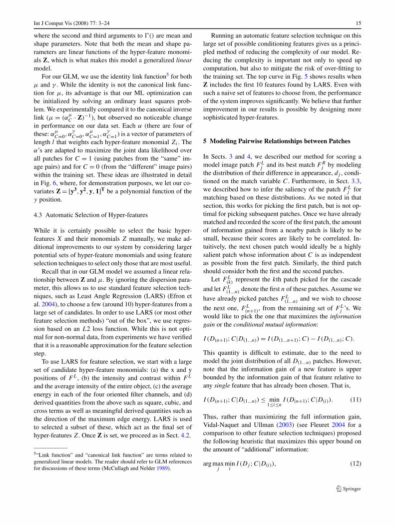
Fig. 8 Patch Correlations. On each image, the patches most corre-lated with the white-circled patch are shown. Notice that in the leftimage, where the patch sits in an area with a highly visible horizontalstructure, the most correlated patches all lie along the horizontal fea-tures. Contrast this with the right image, showing correlation of patcheswith a patch sitting on a wheel, where the most correlated patches arethose that strictly overlap the white-circled patch

on the log likelihood ratio sum R that can be applied aftereach patch in the sequence has been matched and its scoreadded to R (see Sect. 3.2).

We assume that we are given a global threshold λ (seeSect. 3.2) that defines a global choice between selectivityand sensitivity. What remains is the definition of thresholdsat each step, λC=1

(k) and λC=0(k) , which allow the system to ac-

cept (declare “same”) if R > λC=1(k) or reject (declare “differ-

ent”) if R ≤ λC=1(k) . If neither of these conditions is met, the

system should continue by comparing the k + 1th patches ofeach image.

To learn these thresholds, we generate identifiers on theleft training images and run the resulting identifier compar-ing against the right images of our training data set. Thiswill produce a performance curve for each choice of k, thenumber of patches included in the classification score, in-cluding k = m, the sum for which λ is defined. Our goalfor the cascade is to make decisions as early as possible butto avoid increasing the error on the training set. These twoconstraints exactly define the thresholds λC=1

(k) and λC=0(k) :

1. For each “same” and “different” pair in the training set(a) generate an identifier with a sequence of m patches

based on IL

(b) classify IR by evaluating

R =m∑

j=1

logP(Dj = dj |C = 1)

P (Dj = dj |C = 0)> λ.

2. Let IC=1 be the set of correctly classified “same” pairs(where label is “same” and R > λ). Set the rejectionthreshold λC=0

(k) by

λC=0(k) = min

IC=1

k∑

j=1

logP(Dj = dj |C = 1)

P (Dj = dj |C = 0).

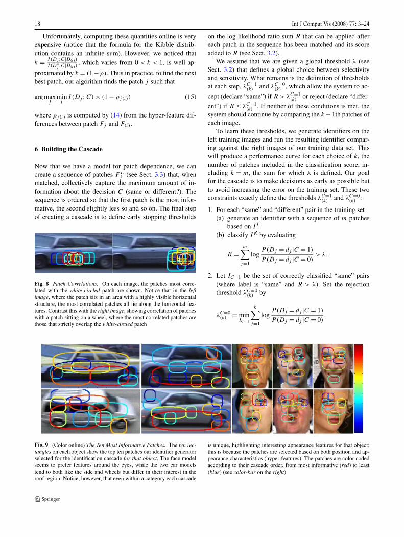
Fig. 9 (Color online) The Ten Most Informative Patches. The ten rec-tangles on each object show the top ten patches our identifier generatorselected for the identification cascade for that object. The face modelseems to prefer features around the eyes, while the two car modelstend to both like the side and wheels but differ in their interest in theroof region. Notice, however, that even within a category each cascade

is unique, highlighting interesting appearance features for that object;this is because the patches are selected based on both position and ap-pearance characteristics (hyper-features). The patches are color codedaccording to their cascade order, from most informative (red) to least(blue) (see color-bar on the right)

Int J Comput Vis (2008) 77: 3–24 19

That is, we want λC=0(k) to be as large as possible without

misclassifying any additional “same” pairs over the baseidentifier which uses all patches.

3. Similarly define IC=0, and set λC=1(k) using the max.

7 Results

The goal of this work is to create an identification systemthat could be applied to different categories, where the algo-rithm would automatically learn (based on off-line trainingexamples) how to select category-specific salient featuresfrom a new image. In this section, we demonstrate that aftercategory training, our algorithm is in fact able take a singleimage of a novel object and solely based on it create a highlyeffective “same” vs. “different” classification cascade of im-age patches. Specifically, we wish to show that for visualidentification each of the following leads to an improvementin performance in terms of accuracy and/or computationalefficiency:

1. breaking the object up into patches, matching each oneseparately and combining the results,

2. differentiating patches by estimating a scoring and sa-liency function for each patch (based on its hyper-features),

3. modeling the dependency between patches to create a se-quence of patches to be examined in order, and

4. applying early termination thresholds to the patch se-quence to create the cascade.

We tested our algorithm on three different data sets: (1)cars from two cameras with significant pose differential, (2)faces from news photographs, and (3) cars from a wide-areatracking system with 33 cameras and 1000’s of unique ve-hicles. Examples from these three data sets are shown inFig. 9, with the top 10 patches of the classification cascade.Notice that the sequence of patches for each object reflectsboth category knowledge (for cars, the system tends to selectdescriptive patches on the side with strong horizontal gradi-ents and around the wheels, while for faces the eyes andeyebrows are preferred) and object specific characteristics.

For each data set, a different automatic preprocessingstep was applied to detect objects and approximately alignthem. After this, the same identification algorithm was ap-plied to all three sets. For lack of space, we detail our ex-periments on data set 1, enumerate the results of data set 2,and only summarize our experience with data set 3. Qualita-tively, our results on the three are consistent in showing thateach of the above aspects of our system improves the per-formance, and that the overall system is both efficient andeffective.

7.1 Cars 1

358 unique vehicles (179 training, 179 test) were extractedusing a blob tracker from 1.5 hours of video from two cam-eras located one block apart. The pose of the cameras rela-tive to the road (see Fig. 1) was known from static cameracalibration, and alignment included warping the sides of thevehicles to be approximately parallel to the image plane. Ad-ditionally, by detecting the wheels, we rescaled each vehicleto be the same length (inter-wheel distance of 150 pixels).This last step actually hurts the performance of our system,as it throws away size as a cue (the camera calibration givesus a good estimate of actual size). However, we wanted todemonstrate the performance when such calibration infor-mation is not available (this is similar to our face data set,where each face has been normalized to a canonical size).

Within training and testing sets, about 2685 pairs (trueto false ratio of 1:15) of mismatched cars were formed fromnon-corresponding images, one from each camera. These in-cluded only those car pairs that were superficially similar inintensity and size. Using the best whole image comparisonmethod we could find (normalized correlation on blurred fil-ter outputs) on this set produces 14% false positives (29%precision) at a 15% miss rate (85% recall). Example cor-rect and incorrect classification results using our cascade areshown in Fig. 10. This data set together with more exampleresults are available from our web site.

Figure 12 compares several versions of our model byplotting the false-positive rate (y-axis) with a fixed miss rateof 15% (85% recall), for a fixed budget of patches (x-axis).The 85% recall point was selected based on Fig. 11, by pick-ing the equal precision-recall point given the 1 to 15 true-to-false ratio.

The Random Order curve uses our hyper-feature modelfor scoring, but chooses the patches randomly. By com-paring this curve to its neighbors, notice the performancegain associated with differentiating patches based on hyper-features both for scoring (No Hyper-Features vs. RandomOrder) and for patch selection (Random Order vs. FullModel). Comparing Mutual Information vs. Full Modelshows that modeling patch dependence is important forchoosing a small number of patches (see range 5-20) that to-gether have high information content (Sect. 5). ComparingPosition Only (which only uses positional hyper-features)vs. Full Model (which uses both positional and appearancehyper-features) shows that patch appearance characteristicsare significant for both scoring and saliency estimation. Fi-nally, the cascade performs (1.02% error, with mean of 4.3patches used) as well as the full model and better than anyof the others, even when those are given an unlimited com-putation budget.

Figure 11 shows another way to look at the performanceof our full model given a fixed patch (computation) budget

20 Int J Comput Vis (2008) 77: 3–24

Fig. 10 (Color online) Model-Test Car Image Pairs. Each pair of im-ages shows a model and a test image, which has been labeled as “same”or “different” (see upper left corner of test image) by our algorithm.The patches that were used in the cascade for that test image are indi-cated for each pair, where the order is color coded from red to blue.The first 3 rows show correct classification results, while the last 2demonstrate errors. False-negative errors primarily occur with darkercars where the main source of features are the illumination artifactsthat can vary greatly between the images. False-positive errors tend toinvolve very similar cars

(the Conditional MI curve of Fig. 12 represents the intersec-tion of these curves with the 85% recall line). The cascadeperformance is also plotted here (follow the black arrow).The distribution of the number of patches it took to make adecision in the cascade model is plotted in Fig. 13.

7.2 Faces

We used a subset of the “Faces in the News” data set de-scribed in Berg et al. (2004), where the faces have been au-tomatically detected from news photographs and registeredby their algorithm. Our training and test sets each used 103different people, with two images per person. This is an ex-tremely difficult data set for any identification algorithm,as these face images were collected in a completely uncon-trolled manner (news photographs).

Table 1 summarizes our results for running the same al-gorithm as above on this set. Note the same pattern as above:the patch based system generally outperforms whole ob-

Fig. 11 Precision vs. Recall Using Different Numbers of Patches(Cars 1). These are precision vs. recall curves for our full model. Eachcurve represents the performance tradeoff between precision and recall,when the system uses a fixed number of patches. The lowest curve usesonly the single most informative patch, while the top curve uses up to100 patches. The 85% recall rate, where the different models of Fig. 12are compared, is noted by a vertical black dashed line. A magenta X,at recall = 84.9 and precision = 84.8, marks the performance of thecascade model

Table 1 Precision vs. recall for faces

Recall Rate 60% 70% 80% 90%

PCA + MahCosine 82% 73% 62% 59%

Filter + NormCor 83% 73% 67% 57%

No Hyper-Features 86% 73% 68% 62%

Random 10 Patches 79% 71% 64% 60%

Top 1 CMI Patch 86% 76% 69% 63%

Top 50 CMI Patches 92% 84% 75% 67%

CMI Cascade 92% 84% 76% 66%

Each column denotes the precision associated with a given recall ratealong the P-R curve. PCA + MahCosine and Filter + NormCor arewhole face comparison techniques. PCA + MahCosine is the best curveproduced by (Bolme et al. 2003), which implements PCA and LDAalgorithms with face-specific preprocessing. Filter + NormCor usesthe same representation and comparison method as our patches, butapplied to the whole face. The last four all use our patch based systemwith hyper-features. The last three use conditional mutual informationbased patch selection, where the number of patches allowed is set to 1,50, and variable (cascade), respectively. These cascades use between 4and 6 patches on average to make a decision.

ject systems (here we compare against state of the art PCAand LDA algorithms with face specific preprocessing us-ing CSU’s implementation Bolme et al. 2003); estimating ascoring and saliency function through hyper-features greatlyimproves the performance of the patch based system; thecascades, using less than 6 patches on average, performs aswell as always using the best 50 patches (performance ac-tually declines above 50 patches). Refer to Fig. 14 for ex-

Int J Comput Vis (2008) 77: 3–24 21

Fig. 12 (Color online) Comparing Performance of Different Models(Cars 1). The curves plot the performance of various models, as mea-sured by the false-positive rate (fraction of different pairs labeled incor-rectly as same), at a fixed recall rate of 85%. The y-axis shows the logerror rate, while the x-axis plots the log number of patches the modelswere allowed to use (up to a max of 100). As the number of patchesincreases, the performance improves until a point, after which it lev-els off and, for the models that order patches according to informationgain, even decreases (when non-informative patches begin to pollutethe score). The top line uses no hyper-features (i.e. uses the same dis-tributions for all patches) and hence performs very poorly compared tothe hyper-feature versions, even when it is allowed to use 100 patches.The second curve from the top uses our hyper-feature model to scorethe patches, but random selection to pick the patch order. The darkblue position only model uses only position (including size: x, y,w,h)based hyper-features for selecting patch order (i.e. it computes a fixedpatch order for all cars but using the same conditional mutual infor-mation algorithm as the full model). The light blue line uses all thehyper-features used by the full model, but sorts the patches by mutualinformation, without considering dependencies (instead, it uses a sim-ple heuristic to prevent selected patches from overlapping too much).The magenta curve shows our full model based on selecting patches ac-cording to their conditional mutual information, using both positionaland image-based hyper-features. Finally, the magenta X at 4.3 patchesand 1.02% error shows the performance of the cascade model

ample classification results. As part of an extension of thiscurrent paper (Jain et al. 2006), we have also compared thisalgorithm to Bayesian face recognition (Moghaddam et al.2000), which won the 1996 FERET face identification com-petition, and found our algorithm to perform significantlybetter on this difficult data set. Our more recent work furtherimproves on the results reported here by training a discrim-inative model on top of the hyper-features.

7.3 Cars 2

We are helping to develop a wide-area car tracking systemwhere this component must re-identify vehicles when theypass by a camera. Detection is performed by a blob trackerand the images are registered by aligning the centroid of theobject mask (the cameras are located approximately perpen-

Fig. 13 How many patches does it take to make a decision? This his-togram shows the number of patches that were matched by the clas-sification cascade before a decision could be made. On average, 4.2patches were required to make a negative (declaring a difference) de-cision, and 6.7 patches to make a positive one

Fig. 14 Model-Test Face Image Pairs. The first two rows of imagesshow correct results, while the bottom two demonstrate errors. Thelarge variations in pose, lighting, expression and image resolutionmake this data set very difficult. Our algorithm prefers eyes and seemsto have learned that when the face is partially in profile, the eye that ismore frontal is more informative (probably because it is more likely tobe consistent)

dicular to the road). We tested our algorithm on a subset ofdata collected from 33 cameras and 1000’s of unique vehi-cles, by learning an identifier generating function for eachcamera pair. In this fashion, the system incorporates the typ-ical distortions that a vehicle undergoes between these cam-eras.

Equal error rates for our classification cascade were3–5% for near lane (vehicle length ∼140 pixels) and 5–7%for far lane (∼60 pixels), using 3–5 patches on average.Whole object comparison methods (we tested several dif-

22 Int J Comput Vis (2008) 77: 3–24

ferent techniques) and using patches without hyper-featuresresulted in error rates that were 2 to 3 times as large.

7.4 Algorithm Complexity

This algorithm was designed to be able to perform real-timeobject identification. The most computationally expensivepart is the off-line training, as many patches must be sam-pled and matched using normalized correlation (3–800,000in our experiments above). For the on-line step, our obser-vation is that a model will be built only once for each cate-gory instance (Step 2 of our algorithm), but that model willthen be applied (matched) many times to incoming images(Step 3). Thus we choose to pay the one-time cost of scan-ning over all candidate patches to build the most efficientclassification cascade possible.

Evaluating the informativeness of all patches within animage is, however, not as computationally daunting as itsounds: computing all of our hyper-features for a patch canbe performed using integral images, making their compu-tation time independent of patch size. Given the vector ofhyper-features for a patch, computing the “same” and “dif-ferent” gamma distributions used by the information mea-sure involves computing 2 dot products (one for each degreeof freedom of the distribution). Finally, the mutual informa-tion measure is computed using a table-lookup based on thegamma parameters.

The most expensive on-line step (by far) is matching thepatches of the cascade in Step 3 by searching for the mostsimilar patch in terms of normalized correlation. Thereforethe on-line running time of our algorithm is directly a func-tion of the average number of patches that must be matchedbefore a decision can be made, and the size of the area thatneeds be searched for the best matching patch. Given thecare with which we pick the patches of our cascade, the av-erage number of patches is typically less then 5 (see above).The search area, on the other hand, depends not on our algo-rithm but the accuracy of object detection method used.

Our current implementation is in Matlab. We estimatethat an optimized implementation of our algorithm would beable to perform the vehicle identification component of thesystem described above with up to five new vehicle reportsper second, and 15 candidate ids per report, in real time ona single processor.

8 Conclusion

We have described a new object identification system thatis general in that it can be applied to different categories ofobjects. We have shown that the key step is to teach the sys-tem to be able to pick informative features for new objectswithin the given category given an off-line labeled category

Fig. 15 Selecting Unusual Features. For each image, the first (mostinformative) patch of the cascade is displayed

training set. Our main contribution is a novel learning algo-rithm that actually models the space of possible features forthe category, allowing it to select and score features that ithas never seen before, based on a single new example.

In the introduction, we have argued that our goal was tobuild an algorithm that has the potential to recognize the use-fulness of a mole on a person’s cheek for identification, evenwhen it had never seen another person with such a mole. Thehope is that the system would be able to generalize fromhaving seen other similar facial blemishes in other locations(that is, in our case, image patches with mole-like appear-ance characteristics), and recognize that such patches, wher-ever they are located, make good features.

While we have no faces with obvious moles in our dataset, Fig. 15 shows two example results that make us hope-ful that we are on the right track. In both, the algorithm haspicked a very atypical patch as its top most informative fea-ture, due to an unusual image characteristic. The left imagecontains the only person in the our data set who is wear-ing sunglasses and it is the only image for which the algo-rithm has decided not to pick a patch near the eyes as its topfeature. The right example shows a truck towing a flatbedtrailer, where the unique connecting area is chosen as thebest feature. We can only hypothesize how the algorithmmade these seemingly correct yet unusual choices.

In both cases the appearance of the features dominatedthe decision: the homogeneous area of the sunglasses re-placed the usually informative eye features, while the elon-gated lines of the trailer are reminiscent of the type of fea-tures that are found to be informative elsewhere. While ac-curacy of these unusual choices are quantitatively very dif-ficult to measure, we believe that the overall performance ofour algorithm is due to this ability to pick the right patchesfor most objects.

Acknowledgements This work was supported by the DARPA CZTSproject. We would like to thank Sarnoff Corporation for the wide areacar tracking data set (“Cars 2”), especially Ying Sang and HarpreetSawhney. From Berkeley, Ryan White provided the face data set andHao Zhang an implementation for LARS. Vidit Jain at UMass Amherstprovided comparison to Bayesian face recognition. Author Learned-Miller was partially supported by NSF CAREER Award IIS-0546666.

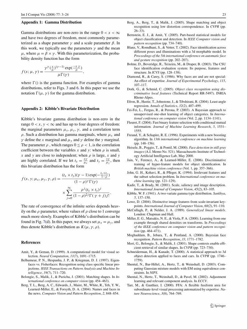
Int J Comput Vis (2008) 77: 3–24 23

Appendix 1: Gamma Distribution

Gamma distributions are non-zero in the range 0 < x < ∞and have two degrees of freedom, most commonly parame-terized as a shape parameter γ and a scale parameter β . Inthis work, we typically use the parameters γ and the meanμ, where μ = β × γ . With this parameterization, the proba-bility density function has the form

f (x;μ,γ ) = γ γ ( xμ)(γ−1) exp(

−x γμ

)

μ�(γ ),

where �() is the gamma function. For examples of gammadistributions, refer to Figs. 3 and 6. In this paper we use thenotation �(μ,γ ) for the gamma distribution.

Appendix 2: Kibble’s Bivariate Distribution

Kibble’s bivariate gamma distribution is non-zero in therange 0 < x,y < ∞ and has up to four degrees of freedom:the marginal parameters μx,μy, γ, and a correlation termρ. Such a distribution has gamma marginals, where μx andγ define the x marginal and μy and γ define the y marginal.The parameter ρ , which ranges 0 ≤ ρ < 1, is the correlationcoefficient between the variables x and y: when ρ is small,x and y are close to independent; when ρ is large, x and y

are highly correlated. If we let tx = xγμx

and ty = yγμy

, thenthis bivariate distribution has the form

f (x, y;μx,μy, γ,ρ) = (tx × ty)(γ − 1) exp(− tx+ty1−ρ

)

(1 − ρ)γ �(γ )

×∞∑

j=0

ρj (tx × ty)j

(1 − ρ)2j�( γ + j)j ! .

The rate of convergence of the infinite series depends heav-ily on the ρ parameter, where values of ρ close to 1 convergemuch more slowly. Examples of Kibble’s distribution can befound in Fig. 7(d). In this paper, we always set μx = μy , andthus denote Kibble’s distribution as K(μ,γ,ρ).

References

Amit, Y., & Geman, D. (1999). A computational model for visual se-lection. Neural Computation, 11(7), 1691–1715.

Belhumeur, P. N., Hespanha, J. P., & Kriegman, D. J. (1997). Eigen-faces vs. Fisherfaces: Recognition using class specific linear pro-jections. IEEE Transactions on Pattern Analysis and Machine In-telligence, 19(7), 711–720.

Belongie, S., Malik, J., & Puzicha, J. (2001). Matching shapes. In In-ternational conference on computer vision (pp. 454–463).

Berg, T. L., Berg, A. C., Edwards, J., Maire, M., White, R., Teh, Y. W.,Learned-Miller, E., & Forsyth, D. A. (2004). Names and faces inthe news. Computer Vision and Pattern Recognition, 2, 848–854.

Berg, A., Berg, T., & Malik, J. (2005). Shape matching and objectrecognition using low distortion correspondence. In CVPR (pp.26–33).

Bernstein, E. J., & Amit, Y. (2005). Part-based statistical models forobject classification and detection. In IEEE Computer vision andpattern recognition (pp. 734–740).

Blanz, V., Romdhani, S., & Vetter, T. (2002). Face identification acrossdifferent poses and illuminations with a 3d morphable model. InProceedings of the 5th international conference on automatic faceand gesture recognition (pp. 202–207).

Bolme, D., Beveridge, R., Teixeira, M., & Draper, B. (2003). The CSUface identification evaluation system: Its purpose, features andstructure. In ICVS (pp. 128–138).

Diamond, R., & Carey, S. (1986). Why faces are and are not special:An effect of expertise. Journal of Experimental Psychology, 115,107–117.

Dork, G., & Schmid, C. (2005). Object class recognition using dis-criminative local features (Technical Report RR-5497). INRIARhone-Alpes.

Efron, B., Hastie, T., Johnstone, I., & Tibshirani, R. (2004). Least angleregression. Annals of Statistics, 32(2), 407–499.

Fei-Fei, L., Fergus, R., & Perona, P. (2003). A Bayesian approach tounsupervised one-shot learning of object categories. In Interna-tional conference on computer vision (Vol. 2, pp. 1134–1141).

Fleuret, F. (2004). Fast binary feature selection with conditional mutualinformation. Journal of Machine Learning Research, 5, 1531–1555.

Freund, Y., & Schapire, R. E. (1996). Experiments with a new boostingalgorithm. In 13th international conference on machine learning(pp. 148–156).

Heisele, B., Poggio, T., & Pontil, M. (2000). Face detection in still grayimages (A.I. Memo No. 521). Massachusetts Institute of Technol-ogy Artificial Intelligence Lab, May 2000.

Jain, V., Ferencz, A., & Learned-Miller, E. (2006). Discriminativetraining of hyper-feature models for object identification. InBritish machine vision conference (Vol. 1, pp. 357–366).

John, G. H., Kohavi, R., & Pfleger, K. (1994). Irrelevant features andthe subset selection problem. In International conference on ma-chine learning (pp. 121–129).

Kadir, T., & Brady, M. (2001). Scale, saliency and image description.International Journal of Computer Vision, 45(2), 83–105.

Kibble, W. F. (1941). A two-variate gamma type distribution. Sankhya,5, 137–150.

Lowe, D. (2004). Distinctive image features from scale-invariant key-points. International Journal of Computer Vision, 60(2), 91–110.

McCullagh, P., & Nelder, J. A. (1989). Generalized linear models.London: Chapman and Hall.

Miller, E. G., Matsakis, N. E., & Viola, P. A. (2000). Learning from oneexample through shared densities on transforms. In Proceedingsof the IEEE conference on computer vision and pattern recogni-tion (pp. 464–471).

Moghaddam, B., Jebara, T., & Pentland, A. (2000). Bayesian facerecognition. Pattern Recognition, 33, 1771–1782.

Mori, G., Belongie, S., & Malik, J. (2001). Shape contexts enable effi-cient retrieval of similar shapes. In CVPR (pp. 723–730).

Schneiderman, H., & Kanade, T. (2000). A statistical approach to 3dobject detection applied to faces and cars. In CVPR (pp. 1746–1759).

Shental, N., Bar-Hillel, A., Hertz, T., & Weinshall, D. (2003). Com-puting Gaussian mixture models with EM using equivalence con-straints. In NIPS.

Shental, N., Hertz, T., Weinshall, D., & Pavel, M. (2002). Adjustmentlearning and relevant component analysis. In ECCV.

Tarr, M., & Gauthier, I. (2000). FFA: A flexible fusiform area forsubordinate-level visual processing automatized by expertise. Na-ture Neuroscience, 3(8), 764–769.

24 Int J Comput Vis (2008) 77: 3–24

Thrun, S. (1996). Explanation-based neural network learning: A life-long learning approach. Dordrecht: Kluwer.

Turk, M., & Pentland, A. (1991). Eigenfaces for recognition. Journalof Cogntive Neuroscience, 3(1), 71–86.

Vidal-Naquet, M., & Ullman, S. (2003). Object recognition with infor-mative features and linear classification. In International confer-ence on computer vision (pp. 281–288).

Viola, P., & Jones, M. (2001). Rapid object detection using a boostedcascade of simple features. In IEEE conference on computer vi-sion and pattern recognition (pp. 511–518).

Weber, M., Welling, M., & Perona, P. (2000). Unsupervised learningof models for recognition. European Conference on Computer Vi-sion, 1, 18–32.

Wiskott, L., Fellous, J., Krüger, N., & von der Malsburg, C. (1997).Face recognition by elastic bunch graph matching. Proceedings7th International Conference on Computer Analysis of Imagesand Patterns, 19(7), 775–779.

Xing, E., Ng, A., Jordan, M., & Russell, S. (2002). Distance metriclearning with application to clustering with side-information. InAdvances in neural information processing systems.

Zhao, W., Chellappa, R., Rosenfeld, A., & Phillips, P. (2003). Facerecognition: A literature survey. ACM Computing Surveys, 35(4),399–458.