dr 4.1: basic methods for collaborative planning · b point cloud segmentation and 3d path planning...
TRANSCRIPT
DR 4.1: Basic methods for collaborative planning
Federico Ferri∗, Mario Gianni∗, Matteo Menna∗, Stefan Wilkes†and FioraPirri∗
∗Alcor Laboratory, Dipartimento di Ingegneria Informatica, Automatica e Ges-
tionale “Antonio Ruberti”- Sapienza Universita di Roma, via Ariosto 25, 00185
Rome, Italy†Fraunhofer IAIS, Sankt Augustin, Germany
〈[email protected]〉Project, project Id: EU FP7 TRADR / ICT-60963Project start date: Nov 1 2013 (50 months)Due date of deliverable: M14Actual submission date: March 2015Lead partner: ROMARevision: finalDissemination level: PU
This document describes the progress status of the research on the devel-opment of formal basis of collaborative planning, focusing on multi-robottask allocation. The report also describes additional research work concern-ing both the consolidation and the improvement of the functionalities of theUGV and UAV, needed for collaboration. The research reported in this doc-ument concerns the WP4 for the Year 1 of the TRADR project. Plannedwork is introduced and the actual work is discussed, highlighting the rele-vant achievements, how these contribute to the current state of the art andto the aims of the project.
1
DR 4.1: Basic methods for collaborative planning Ferri, F. Gianni, M. Menna, Wilkes, S. and Pirri, F.
1 Tasks, objectives, results 61.1 Planned work . . . . . . . . . . . . . . . . . . . . . . . . . . . . . . . . . . . 61.2 Actual work performed . . . . . . . . . . . . . . . . . . . . . . . . . . . . . . 6
1.2.1 Multi-robot task allocation model . . . . . . . . . . . . . . . . . . . 81.2.2 Modeling uncertainty of the augmented reality world in ARE . . . . 91.2.3 Real-time 3D autonomous navigation framework for the UGV . . . . 101.2.4 3D path planning in cluttered and dynamic environments . . . . . . 111.2.5 Probabilistic framework for traversability analysis . . . . . . . . . . 121.2.6 Adaptive Robust 3D Trajectory Tracking for the UGV . . . . . . . . 151.2.7 Three dimensional motion planning for the UAV . . . . . . . . . . . 161.2.8 The stimulus-response framework . . . . . . . . . . . . . . . . . . . . 22
1.3 Relation to the state-of-the-art . . . . . . . . . . . . . . . . . . . . . . . . . 24
2 Annexes 282.1 Menna, Gianni, Ferri, Pirri (2014), “ Real-time Autonomous 3D Navigation
for Tracked Vehicles in Rescue Environments” . . . . . . . . . . . . . . . . . 282.2 Ferri, Gianni, Menna, Pirri (2014), “Point Cloud Segmentation and 3D Path
Planning for Tracked Vehicles in Cluttered and Dynamic Environments” . . 292.3 Ferri, Gianni, Menna, Pirri (2015), “Fast path generation in 3D dynamic
environments” . . . . . . . . . . . . . . . . . . . . . . . . . . . . . . . . . . 302.4 Gianni, Kruijff, Pirri (2014), “ A Stimulus-Response Framework for Robot
Control” . . . . . . . . . . . . . . . . . . . . . . . . . . . . . . . . . . . . . . 312.5 Gianni, Ferri, Menna, Pirri (2014), “Adaptive Robust 3D Trajectory Track-
ing for Actively Articulated Tracked Vehicles (AATVs)” . . . . . . . . . . . 322.6 Gianni (2014), “Multilayered cognitive control for Unmanned Ground Ve-
hicles” . . . . . . . . . . . . . . . . . . . . . . . . . . . . . . . . . . . . . . . 332.7 Ferri, Gianni, Menna, Pirri (2015), “Dynamic obstacles detection and 3D
map updating” . . . . . . . . . . . . . . . . . . . . . . . . . . . . . . . . . . 35
A Real-time Autonomous 3D Navigation for Tracked Vehicles in RescueEnvironments 45
B Point Cloud Segmentation and 3D Path Planning for Tracked Vehiclesin Cluttered and Dynamic Environments 46
C A Stimulus-Response Framework for Robot Control 47
EU FP7 TRADR (ICT-60963) 2

DR 4.1: Basic methods for collaborative planning Ferri, F. Gianni, M. Menna, Wilkes, S. and Pirri, F.
Executive Summary
The key objective of WP4 is to develop the formal methods needed to modelknowledge exchange, knowledge maintenance, information sharing, commonand individual decision structures in order to deploy collaborative planning.In Year 1, we focused on the multi-robot task allocation problem. In thiscontext, we developed a model which manages the assignment of tasks todifferent robots, involved in a mission, under both time and resource con-straints. The proposed task allocation model also deals with task reliabilityand failures. In addition, we extended the Augmented Reality framework,developed in NIFTi, for both training and validating the proposed task al-location model. In Year 1 we also concentrated on both the consolidationand improvement of the basic functionalities of the UGV and UAV, on topof which multi-robot task allocation has been deployed. In particular, wedeveloped a framework for solving the autonomous 3D navigation task forthe UGV. In this framework, we have faced the problem of 3D path plan-ning, based on point cloud clustering and labeling, and motion control forflipper adaptation. We improved this framework with traversability map-ping and dynamic obstacle removal. We developed a unified framework fortrajectory tracking control design, based on both a direct and differentialkinematic model of the UGV, correlating the motion of the robot body withthe motion of the active flippers, in traversal task execution. We proposed anew approach to robot cognitive control design, based on a stimuli-responseframework that models both robots stimuli and the robot decisions to switchamong tasks. Finally, we developed a 3D motion planning and tracking algo-rithm for the UAV. Most of the research work concerning the improvementsof the basic autonomous functionalities of the robots has been performed,together with other WPs, in order to increase both the degree of flexibilityand reliability of the TRADR set-up.
Role of task allocation in TRADR
Task allocation is at the basis of multi-robot collaboration in TRADR. Theproposed model establishes which task is assigned to which robot, as wellas when a robot has to execute its assigned task, under uncertainties abouttask failures. Task allocation builds on the tasks which each robot can effec-tively perform. Each task is formulated on top of the functionalities everyrobot can exhibit. Therefore, while on the one hand it is quite importantbuilding a decisional structure for task allocation; on the other it is crucialto develop a set of basic functionalities which ensures that each robot ofthe TRADR team is effectively able to execute the assigned tasks. Theseconsiderations motivate part of the research work of WP4, jointly performedwith WP1, WP2 and WP3, concerning the consolidation of those baseline
EU FP7 TRADR (ICT-60963) 3
DR 4.1: Basic methods for collaborative planning Ferri, F. Gianni, M. Menna, Wilkes, S. and Pirri, F.
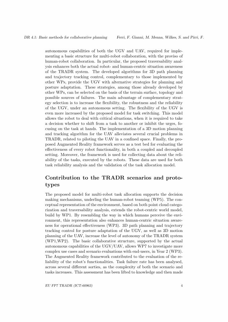
autonomous capabilities of both the UGV and UAV, required for imple-menting a basic structure for multi-robot collaboration, with the proviso ofhuman-robot collaboration. In particular, the proposed traversability anal-ysis enhances both the actual robot- and human-centric situation awarenessof the TRADR system. The developed algorithms for 3D path planningand trajectory tracking control, complementary to those implemented byother WPs, provide the UGV with alternative strategies for planning andposture adaptation. These strategies, among those already developed byother WPs, can be selected on the basis of the terrain surface, topology andpossible sources of failures. The main advantage of complementary strat-egy selection is to increase the flexibility, the robustness and the reliabilityof the UGV, under an autonomous setting. The flexibility of the UGV iseven more increased by the proposed model for task switching. This modelallows the robot to deal with critical situations, when it is required to takea decision whether to shift from a task to another or inhibit the urges, fo-cusing on the task at hands. The implementation of a 3D motion planningand tracking algorithm for the UAV alleviates several crucial problems inTRADR, related to piloting the UAV in a confined space. Finally, the pro-posed Augmented Reality framework serves as a test bed for evaluating theeffectiveness of every robot functionality, in both a coupled and decoupledsetting. Moreover, the framework is used for collecting data about the reli-ability of the tasks, executed by the robots. These data are used for bothtask reliability analysis and the validation of the task allocation model.
Contribution to the TRADR scenarios and proto-types
The proposed model for multi-robot task allocation supports the decisionmaking mechanisms, underling the human-robot teaming (WP5). The con-ceptual representation of the environment, based on both point cloud catego-rization and traversability analysis, extends the robot-centric world model,build by WP1. By resembling the way in which humans perceive the envi-ronment, this representation also enhances human-centric situation aware-ness for operational effectiveness (WP3). 3D path planning and trajectorytracking control for posture adaptation of the UGV, as well as 3D motionplanning of the UAV, increase the level of autonomy of the TRADR system(WP1,WP2). The basic collaborative structure, supported by the actualautonomous capabilities of the UGV/UAV, allows WP7 to investigate morecomplex use cases and scenario evaluations with end-users, in Year 2 (WP3).The Augmented Reality framework contributed to the evaluation of the re-liability of the robot’s functionalities. Task failure rate has been analysed,across several different sorties, as the complexity of both the scenario andtasks increases. This assessment has been lifted to knowledge and then made
EU FP7 TRADR (ICT-60963) 4

DR 4.1: Basic methods for collaborative planning Ferri, F. Gianni, M. Menna, Wilkes, S. and Pirri, F.
persistent, within the multi-robot task allocation model. The role of an in-field rescuer has also been investigated in the problem of allocating tasksamong robots. The presence of an in-field rescuer has been modeled as apositive reward for the robots, in task assignment, as well as a low failurerate, in task execution. Several software packages have been implementedfor traversability analysis, 3D path planning and trajectory tracking controlfor the UGV (analogously for the 3D motion planning for the UAV). Thesepackages contribute to the set up of the TRADR prototype.
EU FP7 TRADR (ICT-60963) 5

DR 4.1: Basic methods for collaborative planning Ferri, F. Gianni, M. Menna, Wilkes, S. and Pirri, F.
1 Tasks, objectives, results
1.1 Planned work
The planned work of WP4, in Year 1, concerning “Basic methods for col-laborative planning” is described in Task T4.1. Task T4.1 achieves theobjectives described in Milestone MS4.1. An excerpt of the description ofboth Task T4.1 and Milestone MS4.1 is reported in the following.
Task T4.1 The goal of Task 4.1 is to develop the formal basis of collab-orative planning, focusing on the early collaborative issues not requiring afull knowledge management. T4.1 expected result at the end of Yr1, is theformalization and implementation of basic collaborative planning methodsfor the generation of a plan common to two or three robots and its execu-tion on an uninstantiated horizon. The model includes a basic memoriesstructuring for both individual and common evaluation of the plan whilemonitoring its execution. A contribution of Task 4.1 is also an augmentedenvironment, with simulated representation, namely an Augmented RealEnvironment (ARE) meant to fill in the lack of a common representation ofthe perceptual data. The novelty of ARE is that it provides the real robot,operating in a real environment, with an augmented reality, by simulat-ing other robots, people, objects, and the knowledge about them is sharedand is made uncertain, replicating noise and incomplete information of realenvironments.
Milestone MS4.1 MS4.1 actuates very basic collaboration performance,providing the early execution model for collaborative planning. The execu-tion to be operated both in real and augmented environment actuates thedifferent levels of knowledge generating and executing a plan. This concernsa common goal for a group formed by one UAV and one UGV. The noveltiesMS4.1 intends to prove are (1) collaborative finding of an unknown target;(2) generation of a common plan handling each other role; (3) compilationof plan results into new knowledge. The last item anticipates major resultsof WP4 on persistence.
1.2 Actual work performed
The actual work performed supports the objectives of Milestone MS4.1. Thiswork focused on the development of a model for multi-robot task allocation.This model establishes which tasks are assigned to robots, as well as when arobot has to execute its assigned task. Task assignment takes into accountboth task failure and reliability due to the occurrence of unknown exogenousevents. The Augmented Reality framework, developed in NIFTi, has beenextended with a probabilistic model for both generating virtual events and
EU FP7 TRADR (ICT-60963) 6

DR 4.1: Basic methods for collaborative planning Ferri, F. Gianni, M. Menna, Wilkes, S. and Pirri, F.
regulating their dynamics. This model served as a ground truth for analysingthe reliability of the tasks, executed by the robots, while the planning scenedynamically changed, being augmented by virtual events. However, multi-robot collaboration presupposed a model of perception, reasoning, planningand execution of the UGV (analogously of the UAV). Such a model builton the effective functionalities, which the robot can exhibit, such as pathplanning, given a suitable representation of the environment, accountingfor the complexity of the terrain, trajectory control for path execution andmorphological adaptation, resource management and task switching, dealingwith the choice of the best task to be executed, when unexpected eventsoccur. Some of these basic functionalities have been developed within NIFTi,jointly with other project partners. However, the actual capabilities of therobot resulted to be still very weak and unreliable to support a collaborativemodel of task planning. Therefore, in Year 1, we also concentrated on boththe consolidation and improvement of the main basic functionalities of theUGV (analogously of the UAV), on top of which multi-collaboration hasbeen implemented. In particular,
• we developed a preliminary framework for solving the autonomous 3Dnavigation task for the UGV. In this framework, we have faced theproblem of 3D path planning, based on 3D map clusterization andlabeling, and motion control for flipper adaptation.
• we improved the framework for 3D autonomous navigation with tra-versability analysis and dynamic obstacle removal. The frameworkalso integrates an extended version of randomized A?, coping withdifficult terrains and complex paths for non-holonomic robots;
• we formalized the problem of traversability analysis within a proba-bilistic framework;
• we proposed a unified framework for trajectory tracking control design,based on both a direct and differential kinematic model of the UGV,correlating the motion of the robot body with the motion of the activeflippers, in traversal task execution;
• we developed a 3D motion planning and tracking algorithm for theUAV.
• we proposed a new approach to robot cognitive control based on astimuli-response framework that models both robots stimuli and therobot decisions to switch among tasks in response or to inhibit stimuli;
In synthesis, this section reports the research carried out by WP4, morespecifically the results in Task T4.1.
EU FP7 TRADR (ICT-60963) 7

DR 4.1: Basic methods for collaborative planning Ferri, F. Gianni, M. Menna, Wilkes, S. and Pirri, F.
1.2.1 Multi-robot task allocation model
In the multi-robot task allocation problem, the goal is to allocate severaltasks amongst members of a team of autonomous robots such that thereare no conflicts, while maximizing the reward received for performing thetasks [36, 85]. The simplest forms of multi-robot task allocation problemin general are combinatorial problems, for which the optimal solution canbe very difficult to be efficiently found [42]. A common approach to deal-ing with this complexity is to use a sequential greedy allocation algorithm,where tasks are allocated by iteratively finding the task-robot pair whichresults in the greatest net reward increase, and allocating that task to thatrobot. Sequential greedy solutions have been shown to provide acceptableapproximations which are typically much faster to compute than the optimalsolution [14].
However, in USAR domain applications several unknown exogenous eventscan occur. These events can either positively or negatively affect the per-formance of the tasks, executed by the robots. If we allow tasks to involveexogenous events the following issues arise: (1) the type of the exogenousevents is unknown a priori; (2) the number of possible exogenous eventswhich can occur is unknown a priori; (3) the behaviors which these exoge-nous events can exhibit are unknown a priori; (4) the number of possiblebehaviors is unknown a priori; (5) when and where an exogenous event canoccur is unknown a priori; (6) the reward for tasks can no longer be assumedknown a priori, since the exogenous events are likely to have influence uponthem and, finally, (7) the reward received for doing a task involving oneexogenous event may not contain any information about future task involv-ing another exogenous event, as each exogenous event may have a differentinfluence on the received reward.
In a multi-robot task allocation problem, all the possible exogenousevents which can occur within a real environment can not be explicitly mod-eled. Moreover, even if we were able to detect these events, we would notbe able to predict the behaviors they are going to exhibit. Both events andbehaviors are not directly observable by the multi-robot team, in a real envi-ronment. What we can directly observe either is the failure or the success ofthe tasks executed, over time, by the multi-robot team. In order to allocatetasks among a team of robots, information from previous tasks successfullycompleted or failed can be effectively used. A possible approach to this issueis to model the task reliability, namely, the ability of the robots to executetasks, under stated conditions for a specified period of time. For exampleif the failure rate of a task, executed by a robot, becomes very high, aftera certain time period, probably that task should be assigned to anotherrobot, whose failure rate, for that specific task and at that time period, islower. Thus, by predicting both the life-cycle and the risks of failures of thetasks, the multi-robot task allocation model can use past tasks successfully
EU FP7 TRADR (ICT-60963) 8
DR 4.1: Basic methods for collaborative planning Ferri, F. Gianni, M. Menna, Wilkes, S. and Pirri, F.
completed involving the robots of the team, to better distribute future tasksamong them, over time.
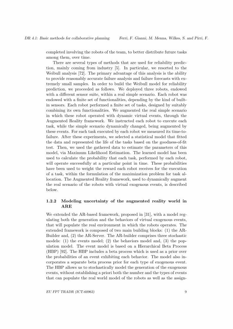
There are several types of methods that are used for reliability predic-tion, mainly coming from industry [5]. In particular, we resorted to theWeibull analysis [72]. The primary advantage of this analysis is the abilityto provide reasonably accurate failure analysis and failure forecasts with ex-tremely small samples. In order to build the Weibull model for reliabilityprediction, we proceeded as follows. We deployed three robots, endowedwith a different sensor suite, within a real simple scenario. Each robot wasendowed with a finite set of functionalities, depending by the kind of built-in sensors. Each robot performed a finite set of tasks, designed by suitablycombining its own functionalities. We augmented the real simple scenarioin which these robot operated with dynamic virtual events, through theAugmented Reality framework. We instructed each robot to execute eachtask, while the simple scenario dynamically changed, being augmented bythese events. For each task executed by each robot we measured its time-to-failure. After these experiments, we selected a statistical model that fittedthe data and represented the life of the tasks based on the goodness-of-fittest. Then, we used the gathered data to estimate the parameters of thismodel, via Maximum Likelihood Estimation. The learned model has beenused to calculate the probability that each task, performed by each robot,will operate successfully at a particular point in time. These probabilitieshave been used to weight the reward each robot receives for the executionof a task, within the formulation of the maximization problem for task al-location. The Augmented Reality framework, used to dynamically augmentthe real scenario of the robots with virtual exogenous events, is describedbelow.
1.2.2 Modeling uncertainty of the augmented reality world inARE
We extended the AR-based framework, proposed in [31], with a model reg-ulating both the generation and the behaviors of virtual exogenous events,that will populate the real environment in which the robots operates. Theextended framework is composed of two main building blocks: (1) the AR-Builder and, (2) the AR-Server. The AR-builder comprises three stochasticmodels: (1) the events model; (2) the behaviors model and, (3) the pop-ulation model. The event model is based on a Hierarchical Beta Process(HBP) [92]. The HBP includes a beta process which is used as a prior overthe probabilities of an event exhibiting each behavior. The model also in-corporates a separate beta process prior for each type of exogenous event.The HBP allows us to stochastically model the generation of the exogenousevents, without establishing a priori both the number and the types of eventsthat can populate the real world model of the robots as well as the assign-
EU FP7 TRADR (ICT-60963) 9

DR 4.1: Basic methods for collaborative planning Ferri, F. Gianni, M. Menna, Wilkes, S. and Pirri, F.
Filtering
Normals Estimation
Segmentation
Labeling
Graph Generation
Inflated Region
Goal Generation
Path Planner
Flipper Position Controller
Trajectory Tracker
Contact Sensor Model
Point Cloud
Principal Curvatures Estimation
Figure 1: Framework overview. Note: solid blocks denote our contribution,while shaded blocks denote third party components.
ment of the behaviors to the events, without fixing a priori which behaviorseach event can exhibit. The model also allows exogenous events within aclass to share the probabilities of exhibiting each behavior, while allowingfor different probabilities across classes. The behavior model is based on aDirichlet Process Gaussian Mixture Model (DP-GMM) [66]. The DP-GMMallows us to model the observed behaviors of the generated exogenous eventswithout assuming that the events exhibit a fixed number of behaviors. Thepopulation model relies on a spatio-temporal Poisson Process to model, inboth time and space, the arrival and leaving of the exogenous events [24].The AR-Server interconnects the real environment model together with thesimulation model of the events [31]. The generated augmented world modelserves as ground truth for training and validating the proposed multi-robottask allocation model, when task reliability of each robot, executing a task,over time, is affected by the presence of exogenous events.
1.2.3 Real-time 3D autonomous navigation framework for theUGV
We developed a framework for 3D path planning and motion control for theUGV. This framework has been integrated into the UGV navigation stack ofTRADR. The main purpose was to extend the autonomous functionalitiesof the UGV, previously developed in NIFTi. On top of all the autonomousfunctionalities of the robot we have built a task library. Such a task libraryhas been used to develop the proposed model of task allocation for multirobot collaboration.
EU FP7 TRADR (ICT-60963) 10
DR 4.1: Basic methods for collaborative planning Ferri, F. Gianni, M. Menna, Wilkes, S. and Pirri, F.
(a) (b)
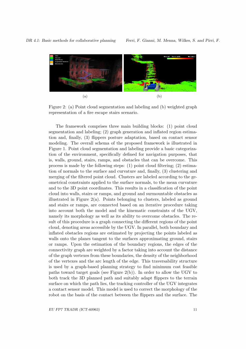
Figure 2: (a) Point cloud segmentation and labeling and (b) weighted graphrepresentation of a fire escape stairs scenario.
The framework comprises three main building blocks: (1) point cloudsegmentation and labeling; (2) graph generation and inflated region estima-tion and, finally, (3) flippers posture adaptation, based on contact sensormodeling. The overall schema of the proposed framework is illustrated inFigure 1. Point cloud segmentation and labeling provide a basic categoriza-tion of the environment, specifically defined for navigation purposes, thatis, walls, ground, stairs, ramps, and obstacles that can be overcome. Thisprocess is made by the following steps: (1) point cloud filtering; (2) estima-tion of normals to the surface and curvature and, finally, (3) clustering andmerging of the filtered point cloud. Clusters are labeled according to the ge-ometrical constraints applied to the surface normals, to the mean curvatureand to the 3D point coordinates. This results in a classification of the pointcloud into walls, stairs or ramps, and ground and surmountable obstacles asillustrated in Figure 2(a). Points belonging to clusters, labeled as groundand stairs or ramps, are connected based on an iterative procedure takinginto account both the model and the kinematic constraints of the UGV,namely its morphology as well as its ability to overcome obstacles. The re-sult of this procedure is a graph connecting the different regions of the pointcloud, denoting areas accessible by the UGV. In parallel, both boundary andinflated obstacles regions are estimated by projecting the points labeled aswalls onto the planes tangent to the surfaces approximating ground, stairsor ramps. Upon the estimation of the boundary regions, the edges of theconnectivity graph are weighted by a factor taking into account the distanceof the graph vertexes from these boundaries, the density of the neighborhoodof the vertexes and the arc length of the edge. This traversability structureis used by a graph-based planning strategy to find minimum cost feasiblepaths toward target goals (see Figure 2(b)). In order to allow the UGV toboth track the 3D planned path and suitably adapt flippers to the terrainsurface on which the path lies, the tracking controller of the UGV integratesa contact sensor model. This model is used to correct the morphology of therobot on the basis of the contact between the flippers and the surface. The
EU FP7 TRADR (ICT-60963) 11

DR 4.1: Basic methods for collaborative planning Ferri, F. Gianni, M. Menna, Wilkes, S. and Pirri, F.
Figure 3: On the left a person is standing in front of a wall (dark blueblob on the left). The white blob behind the person indicates that thepoint cloud of the region of the wall has not been aggregated into the entiremap of the area, due to occlusion. On the right the result of the dynamiccorrection algorithm: after the motion of the person, the map is updatedby both deleting the blob of the person and by aggregating the point cloudbelonging to the wall, previously occluded.
model is based on a learned function, assessing the touch and the detach ofthe flippers from the surface. This approach for flippers control ensures abetter traction of the robot on the terrain, during the trajectory trackingtask. For more details and results concerning this research work we refer toAnnex §2.1.
1.2.4 3D path planning in cluttered and dynamic environments
The framework for real-time 3D autonomous navigation, described above,assumes that the UGV navigates within a static 3D Map. Actually there areno special procedures which are responsible of merging new scans with theaccumulated map, accounting for dynamic obstacle removal, into the map-ping functionalities of TRADR. Therefore, after a short time period, the 3DMap becomes very cluttered, due to the presence of dynamic obstacles, mak-ing the UGV autonomous navigation impossible. Moreover, in the proposedframework, each traversable point within the point cloud was considered asa possible successor state by the planning algorithm. This assumption ex-tremely increases the dimension of the search space, thus breaking down theperformance of the algorithm. In order to face these two main drawbacks,we developed a 3D path planning framework which integrates a procedurefor dynamic obstacle removal as well as a method for sampling candidatesuccessor states so as to reduces the planning domain. The method for test-ing whether a point should be removed is based on a local signed distance
EU FP7 TRADR (ICT-60963) 12

DR 4.1: Basic methods for collaborative planning Ferri, F. Gianni, M. Menna, Wilkes, S. and Pirri, F.
test against the nearest simplex of the convex hull of the scan, acquired fromthe rolling laser sensor. This methods tells us whether a point is inside thedeletion volume [102], also in the presence of noise. The obtained resultis illustrated in Figure 3. Sampling is governed by a probability densityfunction induced by both traversability analysis and obstacle detection. Formore details and results see Annex §2.2 and Annex §2.7. A further improve-ment of this research work is reported in Annex §2.3. In the context ofthe multi-robot collaboration, the proposed dynamic obstacle removal pro-cedure makes both more reliable and effective the autonomous navigationof the UGVs in patrolling tasks.
1.2.5 Probabilistic framework for traversability analysis
During the assessment of the reliability of the UGV navigation task, bal-ancing tasks assignment in the proposed multi-robot task allocation model,we tested the performance of the different algorithms for 3D path planningand trajectory tracking, developed in NIFTi and in WP4 research work. Inthis evaluation we verified that having multiple planning strategies amongwhich the UGV can choose significantly increases both the flexibility androbustness of the overall system. However, safety in navigation tasks wasnot completely ensured. In fact, when the task allocation model assignedthe navigation task to the UGV towards a complex cluttered area of theenvironment, we were forced to manually interrupt the task, in order to pre-vent robot damages. Therefore, the reliability of the UGV navigation taskturns out to be very low, thus bounding tasks assignment. This experienceled us to analyse the problem of autonomous safe navigation. This problemforesees a robot-centric representation of the terrain assessing traversability.Therefore, the research work of WP4 partially pursues to develop a modelfor estimating terrain traversability. This work differs from the researchwork of WP1, concerning adaptive traversability, as it mainly focuses onbuilding a traversability map of the environment, where path planning cantake place, rather than training the controller to adapt the robot flippers todifferent terrain surfaces.
Traversabilty is a continuous scalar metric representing the cost to tra-verse a region. It is usually calculated either from maps or sensor data.Traversability provides a cost map allowing potential obstacles and difficultregions to be avoided at runtime. The cost of traversability is computedcombining geometric features of the neighbourhood of each observation (e.g.,terrain slope, roughness, obstacle presence). Prior works on traversabilitycost estimation do not account for uncertainty and missing information, ina statistically direct manner. Gaussian Processes (GPs) regression have re-cently become popular methods for traversability cost estimation. Thesemethods handle uncertainty as well as appropriately represent spatial cor-relation resulting also effective for managing incompleteness of data. The
EU FP7 TRADR (ICT-60963) 13

DR 4.1: Basic methods for collaborative planning Ferri, F. Gianni, M. Menna, Wilkes, S. and Pirri, F.
(a)
(b)
Figure 4: Figure shows the inference results on synthetic data for terrainsurface (a) and traversabilty cost (b). Top left of each figure shows theoriginal surface, top right shows the observations, bottom left is the inferredsurface and bottom right is the error. The surfaces are jointly learned usingthe multi-task learning framework.
EU FP7 TRADR (ICT-60963) 14

DR 4.1: Basic methods for collaborative planning Ferri, F. Gianni, M. Menna, Wilkes, S. and Pirri, F.
model of terrain produced by GPs is scalable, yielding a continuous domainrepresentation of the terrain data. Moreover sampling can be performed atany desired resolution. However, GPs-based spatial stochastic processes arequite limited when dealing with traversability cost estimation in the presenceof dynamic obstacles. In these settings, time plays an important role for aproper estimation of terrain traversability. In fact, traversabilty mapping ofenvironments with dynamic obstacles requires an update at each time step.Spatial processes, intrinsically memory less, only provide a static represen-tation of the environment, leading to unsatisfactory planning performance.In order to cope with these issues we developed a model for terrain tra-versability, based on spatio-temporal Gaussian Processes, in the context ofmulti-task learning probabilistic framework. Multi-task learning is an areaof machine learning whose goal is to learn multiple related processes avoidingtabula rasa learning by sharing information between the different processes.The main advantage of this approach is to simultaneous learn both theseprocesses in order to the performance over the no transfer case.
Given the set of measures provided by the robot 3D laser sensor and thetraversabilty cost computed on the measured points we infer the model ofboth terrain surface and trasversabilty cost, also taking into account timerelations between different observations. We approached the inference prob-lem by placing a GP prior over the latent process for the terrain surface andthe latent process for the traversabilty cost.
In this model, we defined a covariance function modeling the correlationbetween both the observations of each process and the inter-processes co-variance among the different processes. The latter captures the space-timecorrelation between the processes. This covariance function is stationarywith respect to space but not-stationary with respect to time, in order tomanage local changes on both the terrain surface and the traversability cost,due to the presence of dynamic obstacles. Model parameters are learned bythe maximization of the marginal likelihood of the observations, given boththe inputs and the parameters. The optimization process is constrainedin order to guarantee the properties of the covariance function (e.g., semi-definitive positiveness) as well as to reduce the search space, ensuring real-time reliability. A preliminary result on synthetic data is shown in Figure4.
1.2.6 Adaptive Robust 3D Trajectory Tracking for the UGV
In Annex §2.1 we developed a preliminary trajectory tracking control modelof the UGV. This control model has been evaluated at the Italian FireFighters rescue training area in Prato, during Year 4 of NIFTi, and at var-ious fire-escape and ordinary stairs. In Prato we observed that the robothad locomotion difficulties in rotational motions, when it was autonomouslytraversing narrow passages, due to the flippers in a flat configuration. In
EU FP7 TRADR (ICT-60963) 15

DR 4.1: Basic methods for collaborative planning Ferri, F. Gianni, M. Menna, Wilkes, S. and Pirri, F.
this situation, a better control strategy could have been the decision to liftthe flippers to enhance the robot mobility, instead of maximizing the con-tact surface with the ground. Further, where the terrain was particularlyunstable, the rotation of the belts of the tracks caused ditches in the sand,within which the robot got stuck, due to a loss of both friction and propul-sion. Still, when the robot was passing over holes or gaps, the behavior ofthe flipper position controller was to lower the flippers, as much as possible,causing a bump at the end of the flippers with the negative side of the ob-stacle. If the slope of the negative obstacle was not so steep, the controllerrecovered from this situation. Otherwise, the flippers got stuck under thehole, causing damages to the vehicle. The flipper position controller was notable to suitably adjust the flippers posture due to the lack of a fast feedbackabout the structure of the perceived terrain. To cope with this limitationthe trajectory tracking controller could have had to scale the robot velocitywhile waiting for the feedback to move the sub-tracks and correctly approachthe slope of the negative obstacle. This drawback suggests to jointly modelboth the controllers for skid-steering and the sub-tracks posture adaptation.
The performance obtained at the fire escape stairs scenario, was moreencouraging. The robot, endowed with the decoupled control modules, au-tonomously climbed the stairs, from the basement up to the landing of thesecond flight. However, we noted that oscillations of the heading direction ofthe robot frequently occurred, thus increasing both the lateral and longitu-dinal slippage between the tracks and the ridges of the stairs. The controllergenerated high values of angular velocity in order to accurately track theplanned trajectory, without accounting for slippage compensation. Unfortu-nately, the kinematic model, underlying the trajectory tracking controller,did not take into account the slippage, when the control commands of therobot were generated. Moreover, the flipper position controller, even withthe contact sensor model, was not able to reduce this effect.
On the basis of the lessons learned during this in-field experience, wedeveloped a general preliminary solution for trajectory planning and controlof the UGV. Trajectory planning combines the intrinsic robot characteristicswith the geometric properties of the terrain model. The goal of trajectoryplanning is to negotiate collision-free trajectories taking into account theworkspace of the active flippers of the robot. Trajectory control adaptsthe configuration of the flippers while simultaneously generating the trackvelocities, to allow the vehicle to autonomously follow a given feasible 3Dtrajectory. The control relies on both a direct and differential kinematicmodel of the UGV. The benefit of this approach is to allow the controllerto flexibly manage all the degrees of freedom of the UGV as well as theskid-steering. The differential kinematic model has been designed to extendthe differential drive robot model, described in [29] to compensate the slip-page between the robot tracks and the terrain. Moreover, this model allowsus to derive a feedback control law, which ensures the positional error of
EU FP7 TRADR (ICT-60963) 16
DR 4.1: Basic methods for collaborative planning Ferri, F. Gianni, M. Menna, Wilkes, S. and Pirri, F.
the end points of the front flippers, to converge to zero. This control lawdynamically accounts for both the kinematic singularities of the mechanicalvehicle structure and those vehicle configurations in the neighborhood of asingularity. The designed controller also integrates a strategy selector toreduce both the effort of the flipper servo motors and the traction force onthe robot body, recognizing when the robot is moving on an horizontal planesurface. According to this strategy, rotational motions of the robot, movingwithin narrow passages, are also facilitated.
The main idea behind the design of the controller is to apply both theconcepts and methodologies of robot manipulator kinematics to the UGV,and to extend these methodologies with skid steering principles, accountingfor slippage between the tracks and the ground. The role of the strategyselector is to replicate the behavior of a skilled operator, in situations suchas navigating on flat terrains or traversing a narrow passage. For example,a skilled operator would lift up the robot sub-tracks to increase the mobilityas well as to facilitate rotational motions. Optimization techniques havebeen applied to find a solution to the inverse kinematics of the UGV, in thepresence of singularities [80]. To take into account the closeness of the robotconfiguration to a singular configuration, a heuristic is proposed [13]. Thisreduces the task error when the robot configuration is far from singularities.Finally, a pose refinement technique, exploiting the performance of a DeadReckoning System together with the accuracy of an ICP-based simultaneouslocalization and mapping (SLAM), has been proposed to increase the rateof the control loop [29]. For more details and results see Annex §2.5.
1.2.7 Three dimensional motion planning for the UAV
In NIFTi, the UAV was essentially teleoperated by a human pilot. Con-versely, in TRADR, the UAV is expected to perform tasks, under an au-tonomous setting, in order to jointly collaborate with the UGV during theexecution of a common task. Therefore, the implementation of a 3D mo-tion planning and tracking algorithm for the UAV is crucial in TRADR toinvestigate forms of basic collaborations among heterogeneous robots.
Path planning deals with the search for a valid configuration sequence,which securely moves the UAV through the three dimensional space, to reacha predefined goal position. To solve this problem several steps are necessary.
• Discretization of the configuration space, called C-Space
• Finding a search algorithm
• Tracking of a found path and avoiding obstacles
It is supposed that the estimated position of the UAV is provided astransformation and environment perceptions are continuously available via
EU FP7 TRADR (ICT-60963) 17

DR 4.1: Basic methods for collaborative planning Ferri, F. Gianni, M. Menna, Wilkes, S. and Pirri, F.
Figure 5: Example for an octree representation (right) of a cubic room (left).A node takes one of the follwing states: Free (white), occupied (dark gray)or undefined (gray), which needs to be split again.
a point cloud. Based on this requirements the following algorithms arehardware independent and can be used even in a simulated environment.
C-Space discretization The C-Space discretization is an essential stepto optimize point cloud access times and makes search algorithms more effi-cient. It is known, that the classic three dimensional workspace, representedby the point cloud, needs a lot of space, because each fragment of the en-vironment is stored as a three dimensional point. The configuration spaceis an extension of the workspace. It is the space which includes all possibleconfigurations of the UAV and contains, along the position, the velocity, therotation angle or other configuration vectors. So the C-Space takes a lotmore dimensions than the workspace in general.
To reduce the C-Space, a three dimensional discretization techniquecalled Octree is used. An octree is a tree based data structure which di-vides the configuration space in each dimension. The resulting octets arenow representing a smaller part of the original space and are going to beclassified. The octet can be a node, which is synonymic to an unknown spaceor a leaf. A leaf gets the state free or occupied, based on the perceived en-vironment information. A node can not be classified into a free or occupiedstate and needs to be divided again. This step is iteratively called, till thewhole configuration space is split into octets, which has a defined state.
Figure 5 shows the octree representation of a cubic based model. A clas-sic voxel grid representation, which means a discretization using a fixed size,requires the storage of 512 datapoints. By building an octree based repre-sentation, which combines voxels with the same state, only 25 datapointshave to be stored. In this simple example, a compression rate of 96% isreached. Another advantage of the octree is the option to model a safetyzone in the configuration space. By defining a minimal octet size based onthe UAV diameter, even the smallest obstacle takes the place of the minimal
EU FP7 TRADR (ICT-60963) 18

DR 4.1: Basic methods for collaborative planning Ferri, F. Gianni, M. Menna, Wilkes, S. and Pirri, F.
octet size. This operation is known as the Minkowski sum.
A = A⊕B (1)
The UAV can be handled as a single three dimensional point in furtherpath planning and collision check operations. The C-Space itself is just adefinition of a set containing possible configurations. Each configurationvector, or more exactly its position component, can be validated by simplechecking the corresponding occupation state in the octree representationof the perceived environment. To visualize this model representation, alloccupied voxels are going to be drawn.
Path planning using RRTConnect After the C-Space, respectively theworkspace discretization, the method for finally planning the path throughthe environment can be presented. This planning task is also called globalpath planning. What the keyword global stands for, is shown in the nextparagraph. Due to the high dimensional configuration space, a randombased algorithm is used to plan the configuration sequence for the UAV.This algorithm doesn’t find the optimal path, but it’s able to calculate avalid path in a short period of time.
For random based movement planning in robotics Rapidly-ExploringRandom Trees[52], short RRT, are frequently used. A RRT is a tree baseddata structure build by an incremental algorithm. For K iterations a ran-dom configuration is taken from the C-Space and added to the tree using theextend function. Algorithm 1 implements this extension, which is the mainfunctionality of the RRT based path planning. After choosing a random con-figuration qrand the nearest configuration qnear, which is already connectedto the RRT, is determined. Afterwards the tree will be extended, as shownin Figure 6, from the nearest configuration to the random configuration witha previously defined metric ε, assumed that there are no obstacles betweenthis extension qnew and the already connected configuration qnear.
1 def extend ( tree , q ) :2 q near = neare s t ne i ghbour (q , t r e e )3 i f new conf ig (q , q near , q new ) :4 t r e e . add node ( q new )5 t r e e . add edge ( q near , q new )6 i f q new = q :7 return REACHED8 else :9 return ADVANCED
10 return TRAPPED
Algorithm 1: Extends a RRT by a new, randomly chosen, configuration.
EU FP7 TRADR (ICT-60963) 19

DR 4.1: Basic methods for collaborative planning Ferri, F. Gianni, M. Menna, Wilkes, S. and Pirri, F.
qrand
qinit
qnear
qnew
ϵ
Figure 6: Single iteration of theRRT construction in a two dimen-sional configuration space.
OBST.
Global path
1
15
16
...
...
Figure 7: Highly discretized visu-alization of the DWA approach inthree dimensional space.
The extension ends in one of three defined states. If we have addeda new configuration qnew to the RRT, the state ADVANCED is returned.Otherwise no more configurations are available or can’t be connected tothe tree without passing obstacles. This path is in a TRAPPED state.A special case is, that the new configurations equals the randomly chosenconfiguration. In this case we have found a complete path, which is used inAlgorithm 2 and not part of the basic RRT algorithm.
A modification of the RRT algorithm is presented in the RRTConnect[49]approach and shown in Algorithm 2. Two trees are generated parallel, wherethe first tree has its root in the start configuration and the second treein the goal configuration. The algorithm doesn’t search for a connectionbetween start and goal anymore. It’s searching for a connection betweenthose RRTs. After initializing both trees, tree A is extended by a randomlychosen configuration as explained above. Now the algorithm tries to extendtree B also against this configuration, so the trees always grow into thesame direction. The function connect repeats this extension, til no moreextensions are possible towards this configuration. If an extension connectsthe configuration qnew from tree A and qnew from tree B, the function extendsreturns in the state REACHED, which was explained above. In this case aconnection between the trees, and also a possible path was found.
1 def r r t c o n n e c t ( q s t a r t , q goa l ) :2 t r e e a . i n i t ( q s t a r t )3 t r e e b . i n i t ( q goa l )4 for k = 1 to K:5 q rand = random conf ig (C)
EU FP7 TRADR (ICT-60963) 20
DR 4.1: Basic methods for collaborative planning Ferri, F. Gianni, M. Menna, Wilkes, S. and Pirri, F.
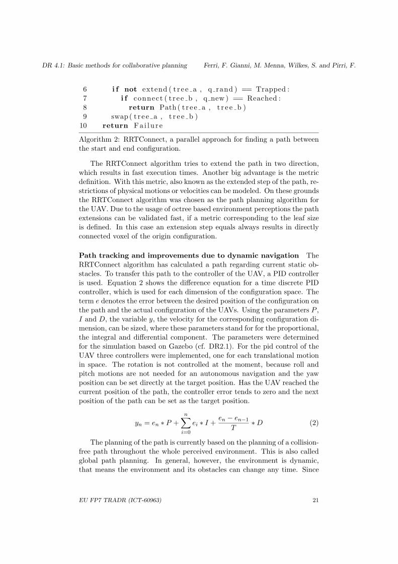
6 i f not extend ( t r e e a , q rand ) == Trapped :7 i f connect ( t r ee b , q new ) == Reached :8 return Path ( t r e e a , t r e e b )9 swap ( t r e e a , t r e e b )
10 return Fa i l u r e
Algorithm 2: RRTConnect, a parallel approach for finding a path betweenthe start and end configuration.
The RRTConnect algorithm tries to extend the path in two direction,which results in fast execution times. Another big advantage is the metricdefinition. With this metric, also known as the extended step of the path, re-strictions of physical motions or velocities can be modeled. On these groundsthe RRTConnect algorithm was chosen as the path planning algorithm forthe UAV. Due to the usage of octree based environment perceptions the pathextensions can be validated fast, if a metric corresponding to the leaf sizeis defined. In this case an extension step equals always results in directlyconnected voxel of the origin configuration.
Path tracking and improvements due to dynamic navigation TheRRTConnect algorithm has calculated a path regarding current static ob-stacles. To transfer this path to the controller of the UAV, a PID controlleris used. Equation 2 shows the difference equation for a time discrete PIDcontroller, which is used for each dimension of the configuration space. Theterm e denotes the error between the desired position of the configuration onthe path and the actual configuration of the UAVs. Using the parameters P ,I and D, the variable y, the velocity for the corresponding configuration di-mension, can be sized, where these parameters stand for for the proportional,the integral and differential component. The parameters were determinedfor the simulation based on Gazebo (cf. DR2.1). For the pid control of theUAV three controllers were implemented, one for each translational motionin space. The rotation is not controlled at the moment, because roll andpitch motions are not needed for an autonomous navigation and the yawposition can be set directly at the target position. Has the UAV reached thecurrent position of the path, the controller error tends to zero and the nextposition of the path can be set as the target position.
yn = en ∗ P +
n∑
i=0
ei ∗ I +en − en−1
T∗D (2)
The planning of the path is currently based on the planning of a collision-free path throughout the whole perceived environment. This is also calledglobal path planning. In general, however, the environment is dynamic,that means the environment and its obstacles can change any time. Since
EU FP7 TRADR (ICT-60963) 21
DR 4.1: Basic methods for collaborative planning Ferri, F. Gianni, M. Menna, Wilkes, S. and Pirri, F.
the dynamic detection of the complete environment is impossible due totechnical difficulties also a second, local navigation approach is required.
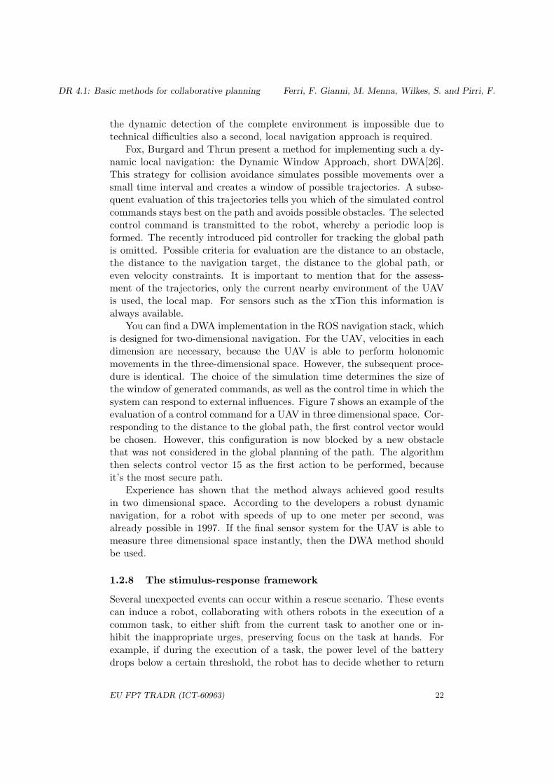
Fox, Burgard and Thrun present a method for implementing such a dy-namic local navigation: the Dynamic Window Approach, short DWA[26].This strategy for collision avoidance simulates possible movements over asmall time interval and creates a window of possible trajectories. A subse-quent evaluation of this trajectories tells you which of the simulated controlcommands stays best on the path and avoids possible obstacles. The selectedcontrol command is transmitted to the robot, whereby a periodic loop isformed. The recently introduced pid controller for tracking the global pathis omitted. Possible criteria for evaluation are the distance to an obstacle,the distance to the navigation target, the distance to the global path, oreven velocity constraints. It is important to mention that for the assess-ment of the trajectories, only the current nearby environment of the UAVis used, the local map. For sensors such as the xTion this information isalways available.
You can find a DWA implementation in the ROS navigation stack, whichis designed for two-dimensional navigation. For the UAV, velocities in eachdimension are necessary, because the UAV is able to perform holonomicmovements in the three-dimensional space. However, the subsequent proce-dure is identical. The choice of the simulation time determines the size ofthe window of generated commands, as well as the control time in which thesystem can respond to external influences. Figure 7 shows an example of theevaluation of a control command for a UAV in three dimensional space. Cor-responding to the distance to the global path, the first control vector wouldbe chosen. However, this configuration is now blocked by a new obstaclethat was not considered in the global planning of the path. The algorithmthen selects control vector 15 as the first action to be performed, becauseit’s the most secure path.
Experience has shown that the method always achieved good resultsin two dimensional space. According to the developers a robust dynamicnavigation, for a robot with speeds of up to one meter per second, wasalready possible in 1997. If the final sensor system for the UAV is able tomeasure three dimensional space instantly, then the DWA method shouldbe used.
1.2.8 The stimulus-response framework
Several unexpected events can occur within a rescue scenario. These eventscan induce a robot, collaborating with others robots in the execution of acommon task, to either shift from the current task to another one or in-hibit the inappropriate urges, preserving focus on the task at hands. Forexample, if during the execution of a task, the power level of the batterydrops below a certain threshold, the robot has to decide whether to return
EU FP7 TRADR (ICT-60963) 22

DR 4.1: Basic methods for collaborative planning Ferri, F. Gianni, M. Menna, Wilkes, S. and Pirri, F.
Task Selection Model
Current Task State
Preconditions
Actions
start
end
Process Statement
Process Statement
start
end
Preconditions
Actions
Constraints
Task Library
Component Component
Knowledge
Planning
Scheduling
Timeline
Timeline
Timeline
Execution Monitoring
Inference
Running Robot Tasks
Process
Process
Process Task State
Stimulus - Response Model yield yield yield
Execution
Features
Environment
Internal State
Stimuli Model
stimulus
stimulus
stimulus
stimulus
Task States
Stimuli–Response Mapping
response
response
response
response
Best Response
Inhibition
Binding
yes
no
continue
Init State
RepresentationLanguage
Reconfiguration
Interference shifting
Explanation
Stimuli Model
Figure 8: Work-flow of the proposed stimulus-response framework. From bottomto top: the lowest layer indicates a current active task, being executed. The activeprocesses feed the processes yields collecting information from them, the stimulimodel selects from the yields those which are stimuli. The stimulus-response modelscores the response tasks. The decision is taken evaluating the payoff of switchingto a task suggested by the stimulus-response matrix. In the middle panel, betweenknowledge and inference, the execution monitoring takes care of the actual taskexecution and its updating, both affecting the mental states, namely the decisionof whether to consent a response to the stimulus. In the upper panel, a first-orderlogical formalism is used to model the robot processes, with action preconditionsand effects, affecting activation costs and motivating causal constraints. This closesthe loop between stimulus activation, reasoning, planning and decision.
EU FP7 TRADR (ICT-60963) 23
DR 4.1: Basic methods for collaborative planning Ferri, F. Gianni, M. Menna, Wilkes, S. and Pirri, F.
to the command base station, to recharge the battery, or to continue thetask. In the first case, the decision to shift to another task can lead to are-allocation of the tasks among all the other robots involved in the commonmission. Therefore, the task allocation model requires a mechanism whichnotifies it when a robot is deviating from the assigned task, due to its in-ternal decision to switch to another task, in order to accordingly re-allocatetasks. This mechanism foresees that each robot is endowed with a cognitiveexecutive control modeling the stimuli identification, the relation betweensuch stimuli and the robot tasks and, finally, the switching decision. Theability to selectively respond to several stimuli, and to inhibit inappropriateurges, focusing on the task at hand, are well-known to exist in humans asshifting and inhibition executive functions [2, 60]. Modeling the dynamicprocesses regulating such cognitive executive functions, in the cognitive ex-ecutive control of the UGV, is crucial to assess a well-regulated behaviourof the robot as well as to balance the work load distributed among themulti-robot team. For this purpose, we developed a preliminary frameworkto model the robot processes, their yields, the stimuli occurrences, and thedecision underlying the response to the stimuli. The proposed frameworkcontributes to the state of the art of robot planning and high level control asit provides a novel perspective on the interaction robot-environment. Themain advantage of this approach is the fact that robot control does not needto be designed a priori but it can be drawn by the interaction with users,who teach the robot when a stimulus is so and what the possible alterna-tives are. Indeed, a robot that has learned a stimulus-response strategy byseveral humans, will most certainly be more usable than a robot that eitherhas no stimuli at all or has no strategies to respond to stimuli, other thanfailures. In fact, we take into account also the context in order to be ableto establish a response cost and we exploit a theory of actions that modelshow tasks are chosen and how a switch to a new task can occur as a result ofa stimulus-response. An overview of the proposed robot stimulus-responseframework is illustrated in Figure 8. During the execution of a task, eachactive robot process yields a quantum of information with characteristic fea-tures; this quantum of information is called the yield of an active process.The features of the yield are used by the stimuli model to learn a functionestablishing whether a stimulus occurred, during the specific process exe-cution, or not. If the stimulus occurs, the robot has to choose a possibleresponse or it can inhibit the stimulus, and continue its task. Therefore therobot has to (1) identify the task that is a possible response to the stimu-lus and (2) decide whether to go on with the current task or to switch tothe identified response task. The first issue is dealt with by filling a scorematrix whose values are estimated via factorization. On the other hand,the switching decision is based on the pay-off of switching. This pay-off iscomputed considering the risk of continuing the current task, without takinginto account the stimulus, and the effort required to fulfil the stimulus. The
EU FP7 TRADR (ICT-60963) 24

DR 4.1: Basic methods for collaborative planning Ferri, F. Gianni, M. Menna, Wilkes, S. and Pirri, F.
effort is, in turn, computed considering two costs: (1) the cost to reconfigurethe current robot state to the new state that switching would lead to and(2) the cost to resolve the interference due to the interruption of the currenttask. These costs are computed by considering the preconditions and effectsof each action involved in both the processes to be interrupted and in theones to be activated. To bind the information yielded by a process to thedomain of reasoning a special functional is used, mapping the process termsof the representation language to the corresponding values of both the yieldsand the stimuli, at execution time. For more details and results see Annex§2.4.
1.3 Relation to the state-of-the-art
Multi-robot task allocation Multi-robot Task Allocation (MRTA) prob-lems seek to allocate tasks to robots such that the cost to complete all tasksis minimised. An extensive amount of work has been proposed to addressmulti-robot task allocation [28, 101, 48]. Methods for solving MRTA prob-lems can be classified into centralized and decentralized approaches, depend-ing by the multi-robot system architecture [9]. Deterministic and heuris-tic approaches based on numerical optimization, dispatching rules, simu-lated annealing, tabu search, genetic algorithms, evolutionary algorithmshave been developed for centralized architecture [78]. On the other hand,behavior-based approaches [75] and market-based approaches [19] have beenproposed for distributed systems [23]. However, an important aspect ofMRTA for multi-robot systems is to take uncertainties in available informa-tion into account when making decisions. Uncertainty can enter the problemat various levels; for example, at the robot level, it may appear as modellinguncertainty resulting from inaccurate models of the robot. Uncertainty alsoenters at the mission level as a result of limited prior knowledge about theenvironment. For example, an accurate model of the environment may notbe available a priori, or the environment might change, making it difficultto decide on the best course of action. Therefore, the proposed approach formulti-robot task allocation attempts to model the uncertainty at the robotmission level by investigating how a class of stochastic reliability modelscan be integrated into typical task allocation frameworks. Task allocationframeworks employing reliability models can results in improved planningperformance when uncertainty enters in task assignment.
Augmented Reality Augmented Reality (AR) is a recent emerging tech-nology stemming from Virtual Reality (VR). AR develops environmentswhere computer-generated 3D objects are blended (registered) onto a realworld scene [3]. This technology has been applied in robotics applica-tions such as maintenance [67], manual assembly [61], computer-assistedsurgery [84], telerobotic control [58], monitoring [1, 7], robot programming
EU FP7 TRADR (ICT-60963) 25

DR 4.1: Basic methods for collaborative planning Ferri, F. Gianni, M. Menna, Wilkes, S. and Pirri, F.
[6, 76, 99, 15], human-robot interaction [98], prototyping [32] and debug-ging [88, 17]. The mentioned approaches for both designing and evaluatingrobotics applications are really very appealing, but, apparently, they do notgo beyond the development of interfaces for overlaying virtual objects intothe real robot scene. Virtual objects can be endowed with simple intelligentbehaviors. Such virtual intelligent objects can be perceived by real robotsas well as can interact with them. Further, the complexity of the real en-vironment can be increased not only by adding virtual objects, but also bymaking vary the behavior of the added objects. Still, complex robot be-haviors can be designed and evaluated, on the basis of the dynamics of thevirtual objects. Under this new perspective, the AR-based framework wehave developed constitutes an important research test-bed for robots meet-ing the needs to test and experiment complex robot behaviors using sucha dynamic and rich perceptual domain. The framework goes beyond thestate-of-the-art concerning AR-based robotic applications, as the design ex-ploits stochastic models activating the behaviors of the introduced objects.Objects, people, obstacles, and any kind of structures in the environmentcan be endowed with a behavior; furthermore, a degree of certainty of theirexistence and behaviors, with respect to what the robot perceives and knowsabout its space, can be tuned according to the experiment needs.
3D autonomous navigation The developed framework for real-time 3Dautonomous navigation for tracked vehicles in rescue environments pro-gressed the current state-of-the-art concerning autonomous 3D mapping andnavigation [56, 45, 16]. Several state-of-the-art approaches make use of 2.5Delevation maps [38] or full 3D voxel maps [45], or point clouds [97], yet at-tempt to reduce the problem dimensionality by planning the paths in a 2Dnavigation map, as also in [47, 63]. The developed framework overcomesthis issues by allowing the UGV to directly plan paths within the 3D mapof the environment. The framework also contributes to the state-of-the-artconcerning 3D Semantic mapping, by building a basic categorization of theenvironment, specifically defined for navigation purposes, based on pointcloud segmentation and labeling [71, 51, 4, 20].
Traversability analysis The proposed model for traversability cost es-timation overcomes the main issues concerning scalability, resolution andcontinuity in domain representation raised from using discrete representa-tions for traversability analysis, based either on elevation maps [35, 37, 77]or on multi-level surface maps [93, 43]. The proposed approach exploitsthe versatility in dealing with uncertainty of Gaussian Process regression[57, 33, 94] together with the commonality property of Multi-Task Learning[50] in order to handle both uncertainty and data incompleteness, in a sta-tistically direct manner. Other popular learning based approaches proposedbinary classification, specifying whether terrain is locally traversable or not
EU FP7 TRADR (ICT-60963) 26

DR 4.1: Basic methods for collaborative planning Ferri, F. Gianni, M. Menna, Wilkes, S. and Pirri, F.
[46, 86, 90]. However, a binary classification is valuable for hazard avoidancebut does not provide any additional information about the cost of regionsand it might be unusable for path planning strategy guidance.
3D Trajectory tracking and control Several research efforts in roboticshave been made to increase the level of autonomy of articulated tracked vehi-cles, focusing on adaptation [34, 65, 73], stability [70, 74], self-reconfiguration[39, 53], track-soil interaction [54, 100] and control [87, 22, 64, 8, 29]. Mostof the proposed solutions focus on a specific task, for example, stair climb-ing rather than rough terrain traversal [34, 65, 44, 73, 53, 70]. Furthermore,most of the proposed approaches to the design of a trajectory tracking con-troller lack a unified framework for modeling the differential kinematics,accounting for all the DOFs of the AATV. The research work, describedin Annex §2.5, advances the state-of-the-art by providing the baselines fordesigning a general adaptive robust 3D trajectory tracking controller foractively articulated tracked vehicles for both skid-steering and sub-tracksposture adaptation, independent of specific tasks.
3D motion planning for UAVs Generally speaking, the state-of-the-artin motion planning is represented by ROS, which provides a comprehensiveframework for the autonomous navigation of a robot of any kind[55][82].However, these algorithms were designed to work in two-dimensional spaceonly. There are several approaches that use these navigation algorithms alsoon a UAV[27] but to the disadvantage of restricted degrees of freedom. Us-ing this methods, a UAV will only be able to navigate safely in one plane.Another framework for path planning is given by MoveIt![40]. Previouslydesigned for classic arm kinematics and related path planning, MoveIt! pro-vides several interfaces, which allow the integration of any robot. A UAVcan also be described as a single point in free space, which can reach anyposition or configuration, physical restrictions not taken into account.
Localization is an essential pre-stage for the autonomous navigation ofa UAV. At this time, a UAV is located either by a motion capturing systemor by its GPS sensor. But in GPS-denied environments there is no positioninformation; hence, other sensors have to be evaluated for their localizationcapabilities. This has been done in a recent Master’s thesis[96] and theresult is presented in more detail in DR2.1.
Cognitive control In the research work, described in Annex §2.4 we ap-plied the well-known concepts of shifting and inhibition in task switching todevelop the executive cognitive control of the UGV [81, 91, 12, 62, 83]. Thetheories on executive cognitive control processes and task switching, initiatedin neuroscience, have strongly influenced cognitive robotics architecturessince the eighties, as for example the Norman and Shallice [69] ATA schemaand the principles of goal directed behaviors in Newell [68]. However only
EU FP7 TRADR (ICT-60963) 27
DR 4.1: Basic methods for collaborative planning Ferri, F. Gianni, M. Menna, Wilkes, S. and Pirri, F.
recently cognitive control is becoming a hot topic in cognitive robotics tomodel a robot complex behavior in unknown environments. Earliest studiesin robotics have been carried within brain-actuated interaction [59], mecha-tronic [10], learning [41] and planning [25]. More recently, several studieshave highlighted the need to model task switching to cope with adaptivityand ecological behaviors in a dynamic environment [11, 89, 95, 21, 18, 30, 79].The major problem to be resolved in most of the cited works, as noted in[95], is the switching decision. Our research work in cognitive control con-tributes to this problem by proposing a solution to model this decision. Inparticular, we modeled the switching decision on the basis of the cost re-sulted from the interplay between the resources needed to reconfigure therobot internal state for the execution of a new task and the resources neededto resolve interference with the current robot internal state [62].
EU FP7 TRADR (ICT-60963) 28

DR 4.1: Basic methods for collaborative planning Ferri, F. Gianni, M. Menna, Wilkes, S. and Pirri, F.
2 Annexes
2.1 Menna, Gianni, Ferri, Pirri (2014), “ Real-time Au-tonomous 3D Navigation for Tracked Vehicles in RescueEnvironments”
Bibliography Matteo Menna, Mario Gianni, Federico Ferri, Fiora Pirri.“Real-time Autonomous 3D Navigation for Tracked Vehicles in Rescue En-vironments.” In Proceedings of the IEEE/RSJ International Conference onIntelligent Robots and Systems (IROS ’14), page 696-702. Chicago, Illinois,2014.
Abstract The paper presents a novel framework for 3D autonomous nav-igation for tracked vehicles. The framework takes care of clustering andsegmentation of point clouds, traversability analysis, autonomous 3D pathplanning, motion planning and flippers control. Results illustrated in anexperiment section show that the framework is promising to face harsh ter-rains. Robot performance is proved in three main experiments taken in atraining rescue area, on fire escape stairs and in a non-planar testing environ-ment, built ad-hoc to prove 3D path planning functionalities. Performancetests are also presented.
Relation to WP This work consolidates the main functionalities of theUGV, on top of which collaborative planning, in Task, T4.1, is developed.
Availablity Unrestricted. Included in the public version of this deliver-able.
EU FP7 TRADR (ICT-60963) 29

DR 4.1: Basic methods for collaborative planning Ferri, F. Gianni, M. Menna, Wilkes, S. and Pirri, F.
2.2 Ferri, Gianni, Menna, Pirri (2014), “Point Cloud Seg-mentation and 3D Path Planning for Tracked Vehiclesin Cluttered and Dynamic Environments”
Bibliography Federico Ferri, Mario Gianni, Matteo Menna, Fiora Pirri.“Point Cloud Segmentation and 3D Path Planning for Tracked Vehicles inCluttered and Dynamic Environments.” In Proceedings of the 3rd IROSWorkshop on Robots in Clutter: Perception and Interaction in Clutter.Chicago, Illinois, 2014.
Abstract The paper presents a framework for tracked vehicle 3D pathplanning in rough areas, with dynamic obstacles. The framework pro-vides methods for real-time point cloud interpretation, segmentation andtraversabilty analysis tacking also into account changes such as dynamic ob-stacles and provides a terrain structure interpretation. Moreover the paperpresents R2A
? an extended version of randomized A? coping with difficultterrains and complex paths for non-holonomic robots.
Relation to WP This work contributes to build the bases for developingformal methods of collaborative planning, in Task, T4.1.
Availablity Unrestricted. Included in the public version of this deliver-able.
EU FP7 TRADR (ICT-60963) 30
DR 4.1: Basic methods for collaborative planning Ferri, F. Gianni, M. Menna, Wilkes, S. and Pirri, F.
2.3 Ferri, Gianni, Menna, Pirri (2015), “Fast path genera-tion in 3D dynamic environments”
Bibliography Federico Ferri, Mario Gianni, Matteo Menna, Fiora Pirri.“Fast path generation in 3D dynamic environments.” Submitted paper.Alcor Laboratory, DIAG “A. Ruberti”, Sapienza University of Rome.
Abstract In this article we present a method for planning paths in 3Denvironments with dynamic obstacles, which is a challenging problem forautonomous robots operating in unstructured environments. Our contribu-tion consists of dynamic obstacles removal and merging of 3D maps, tra-versability analysis within a probabilistic framework, and a domain specificrandomized 3D path planner, which is a further refinement of R2A
?. Resultsshow a performance comparison with other path planners, and evaluationof the dynamic obstacle removal algorithm.
Relation to WP This work improves the main functionalities of theUGV, which constitute the ground for collaborative planning in T4.1.
Availablity Restricted. Not included in the public version of this deliv-erable.
EU FP7 TRADR (ICT-60963) 31
DR 4.1: Basic methods for collaborative planning Ferri, F. Gianni, M. Menna, Wilkes, S. and Pirri, F.
2.4 Gianni, Kruijff, Pirri (2014), “ A Stimulus-ResponseFramework for Robot Control”
Bibliography Mario Gianni, Geert-Jan M. Kruijff, Fiora Pirri. “A Stimulus-Response Framework for Robot Control.” In ACM Transaction on Interac-tive Intelligent Systems, Volume 4, Issue 4, January 2015.
Abstract We propose in this paper a new approach to robot cognitivecontrol based on a stimulus-response framework that models both a robotsstimuli and the robots decision to switch tasks in response or to inhibit thestimuli. In an autonomous system, we expect a robot to be able to deal withthe whole system of stimuli and to use them to regulate its behavior in real-world applications. The proposed framework contributes to the state of theart of robot planning and high-level control in that it provides a novel per-spective on the interaction between robot and environment. Our approachis inspired by Gibsons constructive view of the concept of a stimulus andby the cognitive control paradigm of task switching. We model the robotsresponse to a stimulus in three stages. We start by defining the stimulias perceptual functions yielded by the active robot processes and learnedvia an informed logistic regression. Then we model the stimulus-responserelationship by estimating a score matrix, which leads to the selection ofa single response task for each stimulus, basing the estimation on matrixlow-rank factorization. The decision about switching takes into accountboth an interference cost and a reconfiguration cost. The interference costweighs the effort of discontinuing the current robot mental state to switchto a new state, while the reconfiguration cost weighs the effort of activatingthe response task. A choice is finally made, based on the payoff of switch-ing. Because processes play such a crucial role both in the stimulus modeland in the stimulus-response model, and because processes are activated byactions, we address also the process model, which is built on a theory ofaction. The framework is validated by several experiments, exploiting a fullimplementation on an advanced robotic platform, and compared with twoknown approaches to replanning. Results demonstrate the practical valueof the system in terms of robot autonomy, flexibility and usability.
Relation to WP This work contributes to build the bases for developingformal methods of collaborative planning, in Task, T4.1.
Availablity Unrestricted. Included in the public version of this deliver-able.
EU FP7 TRADR (ICT-60963) 32

DR 4.1: Basic methods for collaborative planning Ferri, F. Gianni, M. Menna, Wilkes, S. and Pirri, F.
2.5 Gianni, Ferri, Menna, Pirri (2014), “Adaptive Robust3D Trajectory Tracking for Actively Articulated TrackedVehicles (AATVs)”
Bibliography Mario Gianni, Federico Ferri, Matteo Menna, Fiora Pirri.“Adaptive Robust 3D Trajectory Tracking for Actively Articulated TrackedVehicles (AATVs).” In Journal of Field Robotics, Special Issue on Safety,Security, and Rescue Robotics (SSRR ’2014), December 2014 (to appear inprint).
Abstract A new approach is proposed for an adaptive robust 3D trajec-tory tracking controller design. The controller is modeled for actively ar-ticulated tracked vehicles (AATVs). These vehicles have active sub-tracks,called flippers, linked to the ends of the main tracks, to extend the loco-motion capabilities in hazardous environments, such as rescue scenarios.The proposed controller adapts the flippers configuration and simultane-ously generates the track velocities, to allow the vehicle to autonomouslyfollow a given feasible 3D path. The approach develops both a direct anddifferential kinematic model of the AATV for traversal task execution cor-relating the robot body motion to the flippers motion. The benefit of thisapproach is to allow the controller to flexibly manage all the degrees offreedom of the AATV as well as the steering. The differential kinematicmodel integrates a differential drive robot model, compensating the slip-page between the vehicle tracks and the traversed terrain. The underlyingfeedback control law dynamically accounts for the kinematic singularitiesof the mechanical vehicle structure. The designed controller integrates astrategy selector too, which has the role of locally modifying the rail pathof the flipper end points. This serves to reduce both the effort of the flipperservo motors and the traction force on the robot body, recognizing when therobot is moving on an horizontal plane surface. Several experiments havebeen performed, in both virtual and real scenarios, to validate the designedtrajectory tracking controller, while the AATV negotiates rubbles, stairs andcomplex terrain surfaces. Results are compared with both the performanceof an alternative control strategy and the ability of skilled human operators,manually controlling the actively articulated components of the robot.
Relation to WP This work provided a model for planning and executionof the UGV, in the context of T4.1.
Availablity Restricted. Not included in the public version of this deliv-erable.
EU FP7 TRADR (ICT-60963) 33

DR 4.1: Basic methods for collaborative planning Ferri, F. Gianni, M. Menna, Wilkes, S. and Pirri, F.
2.6 Gianni (2014), “Multilayered cognitive control for Un-manned Ground Vehicles”
Bibliography Mario Gianni. “Multilayered cognitive control for UnmannedGround Vehicles.” PhD Thesis, September 2014.
Abstract Rescue robots have the potentials to assist responders in search-ing for survivors, in rescuing victims, in providing the responders with ageneral situation awareness, in creating a reference of the destroyed environ-ment, in sampling suspicious substances from hazardous sites, in navigatingthrough those areas, inaccessible for humans. In the last decades, rescuerobots participated in many of the most critical environmental disastersaround the world, exhibiting extraordinary abilities in terms of mapping,vision and navigation. In June 2012, at Mirandola, a city of Northern Italy,hit by a tremendous earthquake, we deployed a team of humans and robot toassess damage to historical buildings and cultural artifacts located therein.This in-field experience has been really important because it led us to abetter understanding of what are the main research challenges which arenot yet widely addressed in rescue robotics. The research work of this thesisaims to investigate, in more detail, some of these challenges, providing solu-tions and methodological approaches to the research problems, still opened.In particular, we address the problem of building a meaningful, higher levelrepresentation of unstructured and dynamic environments, from raw data,coming from the robot sensor suite. We also take care of how to formu-late this representation into a domain where decision making and actionplanning can take place. We tackle with the problem of learning the skillsrequired for a robot to perform a rescue task and formulating such skillsinto robot actions and plans. Here, the novelty is to use a wearable device,namely, the Gaze Machine (GM), to address the correspondence issues be-tween the physical embodiments of the firefighter, wearing the GM, and therobot. Further, this thesis investigates the problem of increasing the levelof autonomy of the robot, in low-level, semi-active and cognitive control.In low-level control, we propose an approach to design and develop a con-troller, which endows the robot with the ability to autonomously traverseharsh terrains, climbing stairs, surmounting obstacles, adapting the config-uration of the robot to the underlying surfaces. In semi-active control, wepropose an approach to coordinate the low-level capabilities of the robotand the interaction between the human and robot, under a mixed-initiativeplanning setting. In this approach the main components and activities ofthe robot are explicitly represented as well as the cause-effect relations andthe temporal constraints among the activities. This control model is basedon a logical framework which combines temporal constraint reasoning andaction planning. This framework provides us with a solid logical structureon which to build the set of cognitive functions of the robot. Such func-
EU FP7 TRADR (ICT-60963) 34

DR 4.1: Basic methods for collaborative planning Ferri, F. Gianni, M. Menna, Wilkes, S. and Pirri, F.
tions endows the robot with the ability to flexibly adapt its behavior inresponse to environmental demands and stimuli. To model this ability, wepropose a method for learning the dynamic processes regulating the humaninspired paradigm of shifting and inhibition, underlying the task switchingmechanism. Finally, this thesis proposes an alternative view of AugmentedReality, as a framework to augment the perceptual model of the robot aswell as to build mixed-reality simulation environments, where to validate theperformance of the robot, in terms of vision, motion planning and control.
Relation to WP This work provides an in-field study of the main issuesconcerning both the deployment and the development of Urban Search andRescue robots. The work also proposes a solution to address these issuesand provides an unified model for planning, reasoning and control of UGVs.This model is at the basis of multi-robot collaboration in T4.1.
Availablity Unrestricted. Available for download: http://www.dis.uniroma1.it/~gianni/mydoc/PhDThesis.pdf
EU FP7 TRADR (ICT-60963) 35

DR 4.1: Basic methods for collaborative planning Ferri, F. Gianni, M. Menna, Wilkes, S. and Pirri, F.
2.7 Ferri, Gianni, Menna, Pirri (2015), “Dynamic obstaclesdetection and 3D map updating”
Bibliography Federico Ferri, Mario Gianni, Matteo Menna, Fiora Pirri.“Dynamic obstacles detection and 3D map updating.” Submitted paper.Alcor Laboratory, DIAG “A. Ruberti”, Sapienza University of Rome.
Abstract We present a real time method for updating a 3D map withdynamic obstacles detection. Moving obstacles are detected through ray-casting on spherical voxelization of point clouds. We evaluate the accuracyof this method on a point cloud dataset, suitably constructed for testing ray-surface intersection under relative motion conditions. Moreover, we show thebenefits of the map updating in both robot path planning and navigation inreal world environments, populated by moving people.
Relation to WP This work improves the main functionalities of theUGV, which constitute the ground for collaborative planning in T4.1.
Availablity Restricted. Not included in the public version of this deliv-erable.
EU FP7 TRADR (ICT-60963) 36

DR 4.1: Basic methods for collaborative planning Ferri, F. Gianni, M. Menna, Wilkes, S. and Pirri, F.
References
[1] P. Amstutz and A.H. Fagg. Real time visualization of robot state withmobile virtual reality. In Proc. ICRA, volume 1, pages 241–247, 2002.
[2] A.R. Aron. The neural basis of inhibition in cognitive control. TheNeuroscientist, 13:214–228, 2007.
[3] Ronald Azuma, Yohan Baillot, Reinhold Behringer, Steven Feiner,Simon Julier, and Blair MacIntyre. Recent advances in augmentedreality. IEEE Comput. Graph. Appl., 21(6):34–47, 2001.
[4] P. Biber, H. Andreasson, T. Duckett, and A. Schilling. 3d modelingof indoor environments by a mobile robot with a laser scanner andpanoramic camera. In IROS, volume 4, pages 3430–3435, 2004.
[5] A. Birolini. Reliability Engineering: Theory and Practice. Springer,2013.
[6] R. Bischoff and A. Kazi. Perspectives on augmented reality basedhuman-robot interaction with industrial robots. In Proc. IROS, vol-ume 4, pages 3226–3231, 2004.
[7] V. Brujic-Okretic, J.-Y. Guillemaut, L.J. Hitchin, M. Michielen, andG.A. Parker. Remote vehicle manoeuvring using augmented reality.In Proc. VIE, pages 186 – 189, 2003.
[8] M. Burke. Path-following control of a velocity constrained trackedvehicle incorporating adaptive slip estimation. In Proceedings of theIEEE International Conference on Robotics and Automation, pages97–102, 2012.
[9] Yifan Cai and Simon X. Yang. A survey on multi-robot systems. InWorld Automation Congress (WAC), pages 1–6, June 2012.
[10] G. Capi. Robot task switching in complex environments. In Advancedintelligent mechatronics, 2007 IEEE/ASME international conferenceon, pages 1 –6, 2007.
[11] G. Capi, G. Pojani, and S.-I. Kaneko. Evolution of task switchingbehaviors in real mobile robots. In Innovative Computing Informationand Control, 2008. ICICIC ’08. 3rd International Conference on, page495, 2008.
[12] Cindy Chamberland and Sebastien Tremblay. Task switching and se-rial memory: Looking into the nature of switches and tasks. ActaPsych., 136:137–147, 2011.
EU FP7 TRADR (ICT-60963) 37

DR 4.1: Basic methods for collaborative planning Ferri, F. Gianni, M. Menna, Wilkes, S. and Pirri, F.
[13] S. Chiaverini, B. Siciliano, and O. Egeland. Review of the dampedleast-squares inverse kinematics with experiments on an industrialrobot manipulator. IEEE Transactions on Control Systems Technol-ogy, 2(2):123–134, 1994.
[14] Han-Lim Choi, L. Brunet, and J.P. How. Consensus-based decentral-ized auctions for robust task allocation. Robotics, IEEE Transactionson, 25(4):912–926, 2009.
[15] J. W. S. Chong, S. K. Ong, A. Y. C. Nee, and K. Youcef-Youmi.Robot programming using augmented reality: An interactive methodfor planning collision-free paths. Robotics and Computer-IntegratedManufactoring, 25(3):689–701, June 2009.
[16] Francis Colas, Srivatsa Mahesh, Francois Pomerleau, Ming Liu, andRoland Siegwart. 3d path planning and execution for search and rescueground robots. In IROS, pages 722–727, 2013.
[17] T.H.J. Collett and B.A. MacDonald. Augmented reality visualisationfor player. In Proc. ICRA, pages 3954–3959, 2006.
[18] D.B. D’Ambrosio, J. Lehman, S. Risi, and K.O. Stanley. Task switch-ing in multirobot learning through indirect encoding. In IntelligentRobots and Systems (IROS), 2011 IEEE/RSJ International Confer-ence on, pages 2802 –2809, 2011.
[19] M. Bernardine Dias. Traderbots: A New Paradigm for Robust and Effi-cient Multirobot Coordination in Dynamic Environments. PhD thesis,Carnegie Mellon University, Pittsburgh, PA, USA, 2004. AAI3126923.
[20] James Diebel and Sebastian Thrun. An application of markov randomfields to range sensing. In NIPS, pages 291–298. MIT Press, 2005.
[21] K.T. Durkee, C. Shabarekh, C. Jackson, and G. Ganberg. Flexibleautonomous support to aid context and task switching. In CognitiveMethods in Situation Awareness and Decision Support (CogSIMA),2011 IEEE First International Multi-Disciplinary Conference on,pages 204 –207, 2011.
[22] D. Endo, Y. Okada, K. Keiji, and K. Yoshida. Path following controlfor tracked vehicles based on slip-compensating odometry. In Proceed-ings of the IEEE/RSJ International Conference on Intelligent Robotsand Systems, 2007, pages 2871–2876, 2007.
[23] A. Farinelli, L. Iocchi, and D. Nardi. Multirobot systems: a classifica-tion focused on coordination. IEEE Transactions on Systems, Man,and Cybernetics, Part B: Cybernetics, 34(5):2015–2028, 2004.
EU FP7 TRADR (ICT-60963) 38

DR 4.1: Basic methods for collaborative planning Ferri, F. Gianni, M. Menna, Wilkes, S. and Pirri, F.
[24] Barbel Finkenstadt and Leonhard Held. Statistical Methods for Spatio-Temporal Systems. Chapman & Hall/CRC, 2006.
[25] Alberto Finzi and Fiora Pirri. Representing flexible temporal behav-iors in the situation calculus. In In Proc. of IJCAI, 2005.
[26] D. Fox, W. Burgard, and S. Thrun. The dynamic window approach tocollision avoidance. Robotics Automation Magazine, IEEE, 4(1):23–33,Mar 1997.
[27] M Gabel, T Kruger, and U Bestmann. Design of a quadrotor sys-tem for an autonomous indoor exploration. In IMAV 2014: Inter-national Micro Air Vehicle Conference and Competition 2014, Delft,The Netherlands, August 12-15, 2014. Delft University of Technology,2014.
[28] Brian P. Gerkey and Maja J Mataric. A formal analysis and taxonomyof task allocation in multi-robot systems. The Intl. J. of RoboticsResearch, 23(9):939–954, 2004.
[29] M. Gianni, G. Gonnelli, A. Sinha, M. Menna, and F. Pirri. An aug-mented reality approach for trajectory planning and control of trackedvehicles in rescue environments. In Proceedings of the IEEE Interna-tional Symposium on Safety, Security, and Rescue Robotics, pages 1–6,2013.
[30] M. Gianni, P. Papadakis, F. Pirri, and M. Pizzoli. Awareness in mixedinitiative planning. In AAAI Fall Symposium Series, 2011.
[31] Mario Gianni, Federico Ferri, and Fiora Pirri. Are: Augmented realityenvironment for mobile robots. In Ashutosh Natraj, Stephen Cameron,Chris Melhuish, and Mark Witkowski, editors, Towards AutonomousRobotic Systems, Lecture Notes in Computer Science, pages 470–483.Springer Berlin Heidelberg, 2014.
[32] B. Giesler, T. Salb, P. Steinhaus, and R. Dillmann. Using augmentedreality to interact with an autonomous mobile platform. In Proc.ICRA, volume 1, pages 1009–1014, 2004.
[33] R. Hadsell, J. A. Bagnell, D. Huber, and M. Hebert. Accurate roughterrain estimation with space-carving kernels. In Proc. of Robotics:Science and Systems, 2009.
[34] D.M. Helmick, S.I. Roumeliotis, M.C. McHenry, and L. Matthies.Multi-sensor, high speed autonomous stair climbing. In Proceedingsof the IEEE/RSJ International Conference on Intelligent Robots andSystems, volume 1, pages 733–742, 2002.
EU FP7 TRADR (ICT-60963) 39

DR 4.1: Basic methods for collaborative planning Ferri, F. Gianni, M. Menna, Wilkes, S. and Pirri, F.
[35] M Herbert, C Caillas, Eric Krotkov, In So Kweon, and Takeo Kanade.Terrain mapping for a roving planetary explorer. In ICRA, pages997–1002, 1989.
[36] J. P. How, C. Fraser, K. C. Kulling, L. F. Bertuccelli, O. Toupet,L. Brunet, A. Bachrach, and N. Roy. Increasing autonomy of UAVs.Robotics and Automation Magazine, IEEE, 16(2):43–51, 2009.
[37] A. Howard, Michael J. T., L. Matthies, B. Tang, A. Angelova, andE. Mjolsness. Towards learned traversability for robot navigation:From underfoot to the far field. J. Field Robotics, 23(11-12):1005–1017, 2006.
[38] Karl Iagnemma, Frank Genot, and Steven Dubowsky. Rapid physics-based rough-terrain rover planning with sensor and control uncer-tainty. In ICRA, volume 3, pages 2286–2291, 1999.
[39] Karl Iagnemma, Adam Rzepniewski, Steven Dubowsky, and PaulSchenker. Control of robotic vehicles with actively articulated sus-pensions in rough terrain. Autonomous Robots, 14(1):5–16, 2003.
[40] Sachin Chitta Ioan A. Sucan. Moveit! http://moveit.ros.org. [Online;Checked 2015-01-28].
[41] Masato Ito, Kuniaki Noda, Yukiko Hoshino, and Jun Tani. Dynamicand interactive generation of object handling behaviors by a smallhumanoid robot using a dynamic neural network model. Neural Net-works, 19:323–337, 2006.
[42] L. B. Johnson, S. Ponda, H.-L. Choi, and J. P. How. Asynchronousdecentralized task allocation for dynamic environments. In Proceedingsof the AIAA Infotech@Aerospace Conference, St. Louis, MO, March2011.
[43] D. Joho, C. Stachniss, P. Pfaff, and W. Burgard. Autonomous explo-ration for 3D map learning. In Autonome Mobile Syst., 2007.
[44] A. Kalantari, E. Mihankhah, and S.A.A. Moosavian. Safe autonomousstair climbing for a tracked mobile robot using a kinematics based con-troller. In Proceedings of the IEEE/ASME International Conferenceon Advanced Intelligent Mechatronics, pages 1891–1896, 2009.
[45] Jochen Klaess, Joerg Stueckler, and Sven Behnke. Efficient mobilerobot navigation using 3d surfel grid maps. In ROBOTIK, pages 1–4,May 2012.
[46] K. Konolige, M. Agrawal, M. R. Blas, R. C. Bolles, B. P. Gerkey,J. Sol, and A. Sundaresan. Mapping, navigation, and learning foroff-road traversal. J. Field Robotics, 26(1):88–113, 2009.
EU FP7 TRADR (ICT-60963) 40

DR 4.1: Basic methods for collaborative planning Ferri, F. Gianni, M. Menna, Wilkes, S. and Pirri, F.
[47] Kurt Konolige, Motilal Agrawal, Robert C. Bolles, Cregg Cowan, Mar-tin Fischler, and Brian Gerkey. Outdoor mapping and navigation usingstereo vision. In Exp. Rob., volume 39, pages 179–190. Springer BerlinHeidelberg, 2008.
[48] G. Ayorkor Korsah, Anthony Stentz, and M. Bernardine Dias. Acomprehensive taxonomy for multi-robot task allocation. Int. J. Rob.Res., 32(12):1495–1512, 2013.
[49] J.J. Kuffner and S.M. LaValle. RRT-connect: An efficient approach tosingle-query path planning. In Robotics and Automation. Proceedings.ICRA ’00. IEEE International Conference on, volume 2, pages 995–1001, 2000.
[50] Abhishek Kumar and Hal Daume. Learning task grouping and overlapin multi-task learning. In John Langford and Joelle Pineau, editors,Proceedings of the 29th International Conference on Machine Learn-ing, pages 1383–1390, New York, NY, USA, 2012. ACM.
[51] Jean-Francois Lalonde, Nicolas Vandapel, Daniel F Huber, and Mar-tial Hebert. Natural terrain classification using three-dimensionalladar data for ground robot mobility. JFR, 23(10):839–861, 2006.
[52] Steven M. Lavalle. Rapidly-exploring random trees: A new tool forpath planning. Technical report, Iowa State University, 1998.
[53] N. Li, S. Ma, B. Li, M. Wang, and Y. Wang. An online stair-climbingcontrol method for a transformable tracked robot. In Proceeding of theIEEE International Conference on Robotics and Automation, pages923–929, 2012.
[54] Y. Liu and G. Liu. Track–stair interaction analysis and online tipoverprediction for a self-reconfigurable tracked mobile robot climbingstairs. IEEE/ASME Transactions on Mechatronics, 14(5):528–538,2009.
[55] Eitan Marder-Eppstein, Eric Berger, Tully Foote, Brian Gerkey, andKurt Konolige. The office marathon: Robust navigation in an in-door office environment. In International Conference on Robotics andAutomation, 2010.
[56] Eitan Marder-Eppstein, Eric Berger, Tully Foote, Brian P. Gerkey,and Kurt Konolige. The office marathon: Robust navigation in anindoor office environment. In ICRA, pages 300–307, 2010.
[57] S. Martin, L. Murphy, and P. Corke. Building large scale traversabilitymaps using vehicle experience. Exp. Robotics, 88:891–905, 2013.
EU FP7 TRADR (ICT-60963) 41

DR 4.1: Basic methods for collaborative planning Ferri, F. Gianni, M. Menna, Wilkes, S. and Pirri, F.
[58] P. Milgram, S. Zhai, D. Drascic, and J. Grodski. Applications ofaugmented reality for human-robot communication. In Proc. IROS,volume 3, pages 1467–1472, 1993.
[59] Jose del R. Millan, Frederic Renkens, Josep Mourino, and WulframGerstner. Brain-actuated interaction. Artificial Intelligence, 159:241–259, 2004.
[60] E.K. Miller and J.D. Cohen. An integrative theory of prefrontal cortexfunction. Annual Review of Neuroscience, 24:167–202, 2007.
[61] J. Molineros and R. Sharma. Computer vision for guiding manualassembly. In Assembly and Task Planning IEEE Int. Symposium, 2001.
[62] Stephen Monsell. Task switching. Trends in Cognitive Sciences,7(3):134 – 140, 2003.
[63] Michael Montemerlo, Sebastian Thrun, Hendrik Dahlkamp, and DavidStavens. Winning the darpa grand challenge with an ai robot. InAAAI, pages 17–20, 2006.
[64] S.A.A. Moosavian and A. Kalantari. Experimental slip estimation forexact kinematics modeling and control of a tracked mobile robot. InProceedings of the IEEE/RSJ International Conference on IntelligentRobots and Systems, pages 95–100, 2008.
[65] A. I. Mourikis, N. Trawny, S. I. Roumeliotis, D. M. Helmick, andL. Matthies. Autonomous stair climbing for tracked vehicles. Inter-national Journal of Robotic Research, 26(7):737–758, 2007.
[66] Radford M. Neal. Markov chain sampling methods for dirichlet processmixture models. Journal of Computational and Graphical Statistics,9(2):249–265, 2000.
[67] U. Neumann and A. Majoros. Cognitive, performance, and systemsissues for augmented reality applications in manufacturing and main-tenance. In Proc. IEEE Virtual Reality Annual International Sympo-sium, pages 4 –11, 1998.
[68] A. Newell. Unified theories of cognition. Harvard University Press,1990.
[69] D. A. Norman and T. Shallice. Consciousness and Self-Regulation:Advances in Research and Theory, volume 4, chapter Attention toaction: Willed and automatic control of behaviour. Plenum Press,1986.
EU FP7 TRADR (ICT-60963) 42

DR 4.1: Basic methods for collaborative planning Ferri, F. Gianni, M. Menna, Wilkes, S. and Pirri, F.
[70] M. Norouzi, J.V. Miro, and G. Dissanayake. Planning high-visibilitystable paths for reconfigurable robots on uneven terrain. In Proceedingsof the IEEE/RSJ International Conference on Intelligent Robots andSystems, pages 2844–2849, 2012.
[71] A. Nuchter, H. Surmann, and J. Hertzberg. Automatic model re-finement for 3d reconstruction with mobile robots. In 3DIM, pages394–401, 2003.
[72] P. O’Connor and A. Kleyner. Practical Reliability Engineering. Wiley,2011.
[73] Y. Okada, K. Nagatani, K. Yoshida, S. Tadokoro, T. Yoshida, andE. Koyanagi. Shared autonomy system for tracked vehicles on roughterrain based on continuous three-dimensional terrain scanning. Jour-nal of Field Robot., 28(6):875–893, 2011.
[74] Panagiotis Papadakis. Terrain traversability analysis methods for un-manned ground vehicles: A survey. Engineering Applications of Arti-ficial Intelligence, 26(4):1373–1385, 2013.
[75] L.E. Parker. Alliance: an architecture for fault tolerant multi-robot cooperation. IEEE Transactions on Robotics and Automation,14(2):220–240, 1998.
[76] T. Pettersen, J. Pretlove, C. Skourup, T. Engedal, and T. Lk-stad. Augmented reality for programming industrial robots. In Proc.IEEE/ACM Int. Symp. on Mixed and Augmented Reality, pages 319–320, 2003.
[77] P. Pfaff, R. Triebel, and W. Burgard. An efficient extension to eleva-tion maps for outdoor terrain mapping and loop closing. Int. J. Rob.Res., 26(2):217–230, 2007.
[78] Michael L. Pinedo. Scheduling: Theory, Algorithms, and Systems.Springer Publishing Company, Incorporated, 3rd edition, 2008.
[79] Fiora Pirri and Matia Pizzoli. Knowing, Reasoning, and Acting Essaysin Honour of Hector J. Levesque, volume 16, chapter Inference aboutActions: Levesques view on action ability and Dirichlet processes.Kings College Publications, 2011.
[80] J. Pujol. The solution of nonlinear inverse problems and the levenberg-marquardt method. Geophysics, 72(4):W1–W16, 2007.
[81] R. Rogers and S. Monsell. The costs of a predictable switch betweensimple cognitive tasks. J. of Exp. Psychology: General, 124:207–231,1995.
EU FP7 TRADR (ICT-60963) 43

DR 4.1: Basic methods for collaborative planning Ferri, F. Gianni, M. Menna, Wilkes, S. and Pirri, F.
[82] Ros navigation stack. http://wiki.ros.org/navigation. [Online;Checked 2015-01-28].
[83] J. Rubinstein, D.E. Meyer, and E.Jeffrey. Executive control of cogni-tive processes in task switching. J. of Exp. Psych.: Human Perceptionand Performance, 27(4):763–797, 2001.
[84] Raj Shekhar, Omkar Dandekar, Venkatesh Bhat, Mathew Philip, PengLei, Carlos Godinez, Erica Sutton, Ivan George, Steven Kavic, ReubenMezrich, and Adrian Park. Live augmented reality: a new visual-ization method for laparoscopic surgery using continuous volumetriccomputed tomography. Surgical Endoscopy, 24:1976–1985, 2010.
[85] T. Shima and S. Rasmussen. UAV Cooperative Decision and Control.Society for Industrial and Applied Mathematics, 2009.
[86] M. Shneier, W. Shackleford, T. Hong, and T. Chang. Performanceevaluation of a terrain traversability learning algorithm in the darpalagr program. Technical report, DTIC Document, 2009.
[87] S. Steplight, G. Egnal, Sang-Hack Jung, D.B. Walker, C.J. Taylor, andJ.P. Ostrowski. A mode-based sensor fusion approach to robotic stair-climbing. In Proceedings of the IEEE/RSJ International Conferenceon Intelligent Robots and Systems, volume 2, pages 1113–1118, 2000.
[88] Michael Stilman, Philipp Michel, Joel Chestnutt, Koichi Nishiwaki,Satoshi Kagami, and James Kuffner. Augmented reality for robot de-velopment and experimentation. Technical report, Robotics Institute,2005.
[89] S. Suzuki, T. Sasaki, and F. Harashima. Visible classification of task-switching strategies in vehicle operation. In Robot and Human Inter-active Communication, 2009. RO-MAN 2009. The 18th IEEE Inter-national Symposium on, pages 1161 –1166, 2009.
[90] A. Talukder, R. Manduchi, R. Castano, K. Owens, L. Matthies,A. Castano, and R. Hogg. Autonomous terrain characterisation andmodelling for dynamic control of unmanned vehicles. In IROS, vol-ume 1, pages 708–713 vol.1. IEEE, 2002.
[91] Thea and Ionescu. Exploring the nature of cognitive flexibility. NewIdeas in Psych., 30(2):190 – 200, 2012.
[92] R. Thibaux and M. Jordan. Hierarchical beta processes and the indianbuffet process. In Proceedings of the 11th Conference on ArtificialIntelligence and Statistics (AISTAT), Puerto Rico, 2007.
EU FP7 TRADR (ICT-60963) 44

DR 4.1: Basic methods for collaborative planning Ferri, F. Gianni, M. Menna, Wilkes, S. and Pirri, F.
[93] R. Triebel, P. Pfaff, and W. Burgard. Multi-level surface maps foroutdoor terrain mapping and loop closing. In IROS, 2006.
[94] S. Vasudevan, F. T. Ramos, E. Nettleton, and H. F. Durrant-Whyte.Large-scale terrain modeling from multiple sensors with dependentgaussian processes. In IROS, 2010.
[95] J. Wawerla and R.T. Vaughan. Robot task switching under dimin-ishing returns. In Intelligent Robots and Systems, 2009. IROS 2009.IEEE/RSJ International Conference on, pages 5033 –5038, 2009.
[96] Stefan Wilkes. 3D Navigation for UAVs in GPS denied environ-ments. Master’s thesis, Westphalian University of Applied SciencesGelsenkirchen, January 2015.
[97] Oliver Wulf, Christian Brenneke, and Bernardo Wagner. Colored 2dmaps for robot navigation with 3d sensor data. In IROS, volume 3,pages 2991–2996, 2004.
[98] J.E. Young, E. Sharlin, and J.E. Boyd. Implementing bubblegrams:The use of haar-like features for human-robot interaction. In Proc.CASE, pages 298–303, 2006.
[99] M.F. Zaeh and W. Vogl. Interactive laser-projection for programmingindustrial robots. In Proc. ISMAR, pages 125 –128, 2006.
[100] Karel Zimmermann, Petr Zuzanek, Michal Reinstein, and VaclavHlavac. Adaptive traversability of unknown complex terrain with ob-stacles for mobile robots. In Proceedings of the IEEE InternationalConference on Robotics and Automation, pages 5177–5182, 2014.
[101] Robert Michael Zlot. An Auction-Based Approach to Complex TaskAllocation for Multirobot Teams. PhD thesis, Robotics Institute,Carnegie Mellon University, 5000 Forbes Ave, December 2006.
[102] G. Zolynski, C. Schank, and K. Berns. Point cloud gathering for anautonomous bucket excavator in dynamic surroundings. In Proc. ofthe Comm. Vehicle Techn. Symp., 2012.
EU FP7 TRADR (ICT-60963) 45
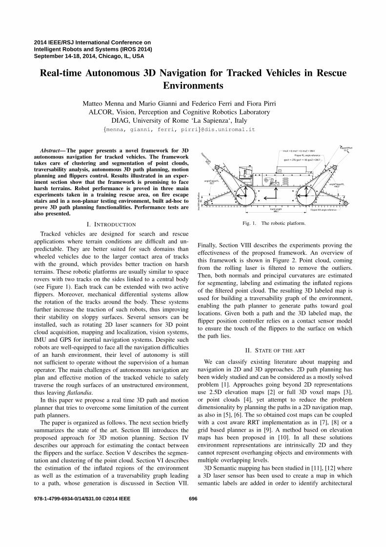
Real-time Autonomous 3D Navigation for Tracked Vehicles in RescueEnvironments
Matteo Menna and Mario Gianni and Federico Ferri and Fiora PirriALCOR, Vision, Perception and Cognitive Robotics Laboratory
DIAG, University of Rome ‘La Sapienza‘, Italy{menna, gianni, ferri, pirri}@dis.uniroma1.it
Abstract— The paper presents a novel framework for 3Dautonomous navigation for tracked vehicles. The frameworktakes care of clustering and segmentation of point clouds,traversability analysis, autonomous 3D path planning, motionplanning and flippers control. Results illustrated in an exper-iment section show that the framework is promising to faceharsh terrains. Robot performance is proved in three mainexperiments taken in a training rescue area, on fire escapestairs and in a non-planar testing environment, built ad-hoc toprove 3D path planning functionalities. Performance tests arealso presented.
I. INTRODUCTION
Tracked vehicles are designed for search and rescueapplications where terrain conditions are difficult and un-predictable. They are better suited for such domains thanwheeled vehicles due to the larger contact area of trackswith the ground, which provides better traction on harshterrains. These robotic platforms are usually similar to spacerovers with two tracks on the sides linked to a central body(see Figure 1). Each track can be extended with two activeflippers. Moreover, mechanical differential systems allowthe rotation of the tracks around the body. These systemsfurther increase the traction of such robots, thus improvingtheir stability on sloppy surfaces. Several sensors can beinstalled, such as rotating 2D laser scanners for 3D pointcloud acquisition, mapping and localization, vision systems,IMU and GPS for inertial navigation systems. Despite suchrobots are well-equipped to face all the navigation difficultiesof an harsh environment, their level of autonomy is stillnot sufficient to operate without the supervision of a humanoperator. The main challenges of autonomous navigation areplan and effective motion of the tracked vehicle to safelytraverse the rough surfaces of an unstructured environment,thus leaving flatlandia.
In this paper we propose a real time 3D path and motionplanner that tries to overcome some limitation of the currentpath planners.
The paper is organized as follows. The next section brieflysummarizes the state of the art. Section III introduces theproposed approach for 3D motion planning. Section IVdescribes our approach for estimating the contact betweenthe flippers and the surface. Section V describes the segmen-tation and clustering of the point cloud. Section VI describesthe estimation of the inflated regions of the environmentas well as the estimation of a traversability graph leadingto a path, whose generation is discussed in Section VII.
flipperLength347,6
trackLength499,7
angleFlipperRL+56,1°
flipperOffset11,1°
angleFlipperFL-56,1°
trac
kWhee
lRad
ius
90
Flipper RR angle reference
imuX = 0; imuY = 0; imuZ = 169.4
Flipper RL angle reference
gpsX = -270; gpsY = -90; gpsZ = 204.7
Fig. 1. The robotic platform.
Finally, Section VIII describes the experiments proving theeffectiveness of the proposed framework. An overview ofthis framework is shown in Figure 2. Point cloud, comingfrom the rolling laser is filtered to remove the outliers.Then, both normals and principal curvatures are estimatedfor segmenting, labeling and estimating the inflated regionsof the filtered point cloud. The resulting 3D labeled map isused for building a traversability graph of the environment,enabling the path planner to generate paths toward goallocations. Given both a path and the 3D labeled map, theflipper position controller relies on a contact sensor modelto ensure the touch of the flippers to the surface on whichthe path lies.
II. STATE OF THE ART
We can classify existing literature about mapping andnavigation in 2D and 3D approaches. 2D path planning hasbeen widely studied and can be considered as a mostly solvedproblem [1]. Approaches going beyond 2D representationsuse 2.5D elevation maps [2] or full 3D voxel maps [3],or point clouds [4], yet attempt to reduce the problemdimensionality by planning the paths in a 2D navigation map,as also in [5], [6]. The so obtained cost maps can be coupledwith a cost aware RRT implementation as in [7], [8] or agrid based planner as in [9]. A method based on elevationmaps has been proposed in [10]. In all these solutionsenvironment representations are intrinsically 2D and theycannot represent overhanging objects and environments withmultiple overlapping levels.
3D Semantic mapping has been studied in [11], [12] wherea 3D laser sensor has been used to create a map in whichsemantic labels are added in order to identify architectural
2014 IEEE/RSJ International Conference onIntelligent Robots and Systems (IROS 2014)September 14-18, 2014, Chicago, IL, USA
978-1-4799-6934-0/14/$31.00 ©2014 IEEE 696

Filtering
Normals Estimation
Segmentation
Labeling
Graph Generation
Inflated Region
Goal Generation
Path Planner
Flipper Position Controller
Trajectory Tracker
Contact Sensor Model
Point Cloud
Principal Curvatures Estimation
Fig. 2. Framework overview. Note: solid blocks denote authors’ contribu-tion, while shaded blocks denote third party components.
elements via geometric features. Research on 3D mappingand reconstruction for mobile robots using laser range finderhas been also explored in [13], [14]. These representations donot make use of any additional semantic label and have notproved to work in real time with a fully autonomous robotsystem, likewise [15], since it is possible to show that stairsare 2D reducible and flipper angles can be set in advance.
Approaches using vision, such as [16], [5], are not directlycomparable to those using 3D sensors as requiring morecomputing effort.
III. 3D MOTION PLANNING
In this section we describe the main components ofthe 3D motion controller designed for a tracked ve-hicle such as the one illustrated in Figure 1. Therobot configuration state is defined by the vector q =(xr,yr,zr,ψ,φ ,θ ,vr,ωr,α1, . . . ,α4)
T , with xr,yr,zr,ψ,φ ,θthe 6D pose of the robot, vr and ωr the linear and angularrobot velocities, respectively. Here, α1, . . . ,α4 are the con-figurations of the robot flipper. The state can be separatedinto two controllable parts, assuming that the control ofthe robot pose is independent of the flippers control. Underthis assumption, the 3D motion planning controller can bedivided into two decoupled control modules: (1) a trajectorytracking controller, and (2) a flippers position controller.These modules work in parallel and are synchronized so asto generate, at time stamp, the control commands neededto track a given 3D path and to simultaneously adapt theposition of the flippers to the surfaces on which the pathlies, namely to the planes tangent at each path point. Thetrajectory tracking controller receives as input a path P(see Section VI), generated on the 3D labeled map of theenvironment (see Section V) and computes the steeringcommands to allow the robot to follow the given path P . Thecontrol strategy underlying the trajectory tracking controlleris based on input-output linearization via feedback [17], [18].The flippers position controller receives the desired flipperpositions αααd(t) = (α1(t), . . . ,α4(t))
T , as input, generatingsuitable internal speed commands to asymptotically stabi-lize to zero the flippers position error, on the basis of aproportional-derivative (PD) control law. The positions αααd(t)are selected from a set of predefined configurations, depend-ing on both the current robot attitude and the information
(a) α f eedback (t) (b) ii(t)
(c) l (t)
Fig. 3. (a) trend of the position of the front right flippers (b) trend ofthe component of the current signal of the front right flippers, in amperes,producing the magnetic field in the desired direction (c) labeling of themeasurements of both α f eedback(t) and ii(t) from the position controller ofthe front right flipper.
provided by the 3D labeled map of the environment [15].These configurations allows the robot to climb stairs andto overcome both positive and negative obstacles. However,during the control loop, the flipper position controller isnot able to detect, after positioning the flippers accordingto the selected posture, whether the flippers effectively areeither in contact with the surface or with the obstacle tobe surmounted. Still, the flippers are neither endowed withcontact sensors nor with proximity sensors. To face this limit,the flipper position controller integrates a statistical modelassessing the touch and the detach of the flippers with thesurface. This model is based on a function, learned froma set of features, extracted from the direct measurementsof both the actual angles ααα f eedback (t) of the flippers (seeFigure 3(a)) and the electrical currents ii(t) of the flipperservo motors (see Figure 3(b)). During the control loop, thecontroller adjusts the flippers posture αααd(t), depending onthe feedback provided by the contact sensor model.
IV. CONTACT SENSOR MODEL
In this section we describe the model of the contact sensorof each flipper. This model is based on learning a functionhθ∗ assessing the optimal position of the flipper.
Data-set collection and labeling Several experimentshave been performed with the robot climbing rampsand stairs, surmounting obstacles, overcoming rubble pileswith different shapes, and several measurements of bothα f eedback (t) and ii(t) of the flipper have been taken, overtime. The gathered data have been manually labeled with alabel l(t) = 1 and l(t) = 0, denoting the touch and the detachof the flipper from the obstacles surfaces, respectively, thusenriching the feedback information provided by the positioncontroller (see Figure 3(c)). This data have been furtherinterpolated to build a data-set D = {〈α(t), ii(t), l(t)〉, t =0, . . . ,T} suitable for the training of the contact sensor model.
Feature representation The data-set D ={〈α(t), ii(t), l(t)〉, t = 0, . . . ,T} has been processed to
697

extract the relevant features for tuning the parameters ofthe function hθ∗ to be learned. Let t ≤ T be a sampled timepoint and let W = [t ′, t] be a fixed sliding time window,with t ′ < t, the following features, inferred from D, can beconsidered as relevant features:
x1 =1
t− t ′t
∑k=t ′|ii(k) |
x2 =1
t− t ′t
∑k=t ′
∣∣∣∣α (k+1)−α (k−1)2
∣∣∣∣x3 = sgn
(t
∑k=t ′
ii(k)
)· sgn
(t
∑k=t ′
α (k+1)−α (k−1)2
)
x4 =1
t− t ′t
∑k=t ′|iiT DF−II (k)|
Here iiT DF−II (t) is the component ii(t) of the currentsignal, filtered according to the Transposed-Direct-Form-II(TDF-II) digital filter. The filter has been applied to reducethe oscillations of ii(t) during the transient conditions ofthe servo drive. The label associated with a feature vectorx = (x1, . . . ,x4)
T is computed as follows:
y =
1 if 1t−t ′
t
∑k=t ′
l (k)> 0.5
−1 otherwise
Let N be the number of sampled time points, then D′ ={(xi,yi)}N
i=1 is the data-set of features-labels pairs generatedfrom D, with xi ∈ X ⊆ R4 and yi ∈ L≡ {−1,1}.
Learning the parameters of hθ∗ Let H = {hθθθ (x) : θθθ ∈Θ} be the space of the decision functions, such that hθθθ : X→L, Θ the parameter space. Given the set D′ = {(xi,yi)}N
i=1of labeled features samples, assumed to be drawn from anunknown distribution P(x,y), we want to find a function hθ∗
which gives the lowest upper bound of the expected risk:
R(θ) =∫|hθθθ (x)− y|P(x,y)dxdy (1)
The lowest upper bound of such a loss function can be foundby applying a non-linear classifier based on the Support Vec-tor Machines (SVM). Therefore the problem of estimatingthe function hθθθ
∗ can be considered as the problem of findingthe decision surface that better separates the data. This canbe formulated as follows:
maximizeθθθ∈Θ
N
∑i=1
θi−12
N
∑i=1
N
∑j=1
yiy jθiθ jK (xi,x j)
subject toN
∑i=1
yiθi = 0,0≤ θi ≤ 1, ∀i = 1, . . . ,N.
Here K (xi,x j) =(xT
i x j +1)d . The polynomial kernel has
been introduced due to the non-linear separability of thedata-set D′. Given a new instance of a feature vector x, thedecision function hθθθ
∗ modeling the contact of the flipper withthe underlying surface classifies x as follows
hθθθ∗ (x) = sgn
(NS
∑i=1
yiθ∗i K (si,x)
)(2)
Fig. 4. Accuracy ratio of the contact sensor model as both the degree dof the polynomial kernel and the sliding time window W change
Here si are the support vectors and θ ∗i are the optimalparameter values associated to si, with i = 1, . . . ,NS. Across-validation technique has been used to evaluate theperformance of the contact sensor model as both the degreed of the polynomial kernel and the sliding time window Wchange. Figure 4 shows that for d = 13 and W = 5 the modelcorrectly classifies 90.7% of the contacts of the flipper withthe underlying surface.
V. POINT CLOUD SEGMENTATION AND LABELING
In this section we describe a real time point cloud PC seg-mentation and labeling, registered by an ICP-based SLAM[19]. The point cloud PC stores the geometric position(x,y,z) of each point p ∈ PC, approximating a surface M.The objective is to establish traversability of the surfacefor the path control, requiring real-time computation. Tothis end we define just four categories for traversability:ground, walls, ramp or stairs, surmountable obstacle. Thesecategories have been specified to match the effective robotovercoming abilities: 30 cm steps with rounded edge; 40cm gap; 20 cm stairs at 40◦ slope; spiral staircases; 45◦
slope / 15◦ roll; 80cm× 80cm cavities. Here we assumethat segmentation is always performed on the incoming lasermeasures, and we consider the current one, in so avoidingto parametrize points with time.
We propose here a novel approach to simple categoriessegmentation based on geometric features. The approach isspecified by the following steps (1) patch construction andfiltering; (2) estimation of the normals and of the principalcurvatures of the surface at all points and (3) segmentationand labeling of the PC.
Patch construction and Filtering An initial points fil-tering is already provided by the ICP algorithm, here weare mainly concerned with constructing a surface patch foreach PC region, used for geometric features computation,and to discard ill-conditioned neighborhoods. A patch isdefined by a mapping ψ : (x,y) 7→M, with ψ(x,y) = p ∈R3,and (x,y) ∈ R2, the parameters of the mapping. To simplifywe denote ψ(x,y) by x intending also the coordinates ofthe point p on the surface M; similarly, we identify theparameters with the x and y coordinates. The patch can beobtained by transforming the point representation of PC into
698

a voxel grid, building a suitable neighborhood for pointsthat can be reordered into surface patches of contiguouspoints, and ensuring that there is none or little overlappingbetween patches. First we decimate the PC of a factor of 0.9to obtain the downsampled PCs, and then we initialize theneighborhood of each point q in PCs with k-means taking theq as seeds, using only the points coordinates together withthe Euclidean distance. Since k-means does not take care ofill-conditioned clusters we adjust each cluster by expandingit or reducing it, by splitting or merging, according to thecluster spatial frequency ρ = |H|/r3, where |·| is the cardinalityof the cluster H and r = mean(d(H)) is the radius definedby the mean distance within the cluster. An optimal densityρ? is given by a radius rmin = 0.5
√2m, (m, meters), and a
neighborhood of 81 points. If ρ < ρ?/2 then r is increasedto catch more points joining with the cluster that ensuresto keep the optimal dimension, among the closer ones. Tocontrol the radius growth and filter out noise, a noise functionis specified according to the spatial frequency of points asfollows. Let ϕ(H) = exp(−π(rmin− r)), then the probabilitythat a neighborhood H is affected by noise is:
p(noise(H)) = 1−ϕ(H) (3)
The noise function is clearly zero when r = rmin. Neigh-borhoods with noise value greater than 0.5 are removedfrom the PC. Once the clusters are stabilized then, eachof them is labeled into a voxel grid, possibly resorting tointerpolation, mostly required at the boundary of a patch,so that close points are contiguous. The grid representationleads to the surface patch representation of the three matricesX, for the x coordinates of the points in the cluster, Y for they coordinates, and Z for ψ(x,y). These matrices have sizem×n each.
Normal and principal curvature estimation Havingtransformed the original PC into a number of surface patcheswell approximating the surface M, using the neighborsconstruction and the grid, a very precise estimation of thenormals, and likewise of the principal curvatures, can beobtained quite simply, using first and second derivatives. Thisallows us to avoid the computation based on least meansquare (see for example [20], [21]), which can be quitesensitive to noise and it is computationally very expensive,since it requires to compute neighborhoods for each point ofthe cloud and to perform SVD decomposition.
Here we consider finite-size linear-phase separable ker-nels, introduced by [22], for first and second order differ-entiation of discrete multidimensional signals. These kernelsare used to convolve the matrices X, Y and Z to obtain thederivatives, by first expanding the matrices at the bound-aries. Then, differentiation for each coordinate x and y isobtained by collecting the convolution of each matrix in eachdirection. Namely, let fx,gx,hx be the first-order derivativesof X, Y and Z, respectively, with respect to x, obtainedwith the convolution kernel, these are matrices of size m×ntoo. Therefore xx is the tensor ( fx,gx,hx)
> and, analogously,xy = ( fy,gy,hy)
>. In an analogous way we obtain the second-
order derivatives xxx, xyy, xxy. Having defined the patches inexplicit form, it is now straightforward to obtain the normalsns for all the points in a patch, by simply applying the crossproduct to the first derivative tensors, obtaining the tensor3×n×m:
±
gx ·hy−gy ·hxfy ·hx− fx ·hyfx ·gy− fy ·gx
(4)
and normalizing to get the tensor N of unit normals,noting that in the above equation · is the element-wisematrix multiplication. Note that the sign can be actuallydetermined by simply computing the smallest angle be-tween the obtained normals and the laser source position,say S . Namely, we look for the angle θ minimizingcos−1(s>n′3×mn)/‖s‖‖n′3×mn‖, where
s = (S ⊗11×nm−x′3×nm)/‖S ⊗11×nm−x′3×nm‖
with S the source position, ⊗ the Kronecker product, x′3×nmand n′3×nm tensors of size (3×n×m) reshaped into a 3×nmmatrix.
As for the principal curvatures, at each point p in apatch, we exploit the fact that with the first and secondderivatives and the normals tensor N available, we canobtain the following elements, named according the I andII fundamental forms:
E = Σdim=3xx ·xx F = Σdim=3xx ·xy G = Σdim=3xy ·xy;L = Σdim=3xxx ·N M = Σdim=3xxy ·N N = Σdim=3xyy ·N
(5)In other words E,F,G,L,M,N are all matrices m×n. Thus,k is computed as the solution of the quadratic equation
(EG−F2)k2 +(2FM−EN−GL)k+(LN−M2) (6)
And it is well-known that the discriminant of the aboveequation is greater or equal zero, therefore there are eithertwo distinct real roots k1 and k2, namely the two principalcurvatures, or a single one. While at umbilical points L/M =M/F = N/G. Given the principal curvatures we can alsoobtain both the mean curvature (1/2)(k1+k2) and the Gaus-sian curvature k1k2. We observe that the only computationaldifficulty here is the construction of the patches. The maindifficulties coming from far points, which are those mostlyrequiring merging and dropping, therefore it might be betterfor those noisy regions to delay the patch construction,according to the noise function defined in (3).
Segmentation and Labeling Segmentation still uses thematrices X,Y,Z yet all integrated into the voxel grid.We note that without hampering the information for thecategories, the kernel convolution included a significantsmoothing of the matrix Z. Then we can obtain from thenormals, the Gaussian curvature and the principal curvaturesan initialization of the categories as follows. Let |n| =(|n1|, |n2|, |n3|)> be the unit normal absolute value at a pointp, let K = k1k2 be the Gaussian curvature, with k1 and k2the principal curvatures, let θ1 = 0.17 and θ2 = 0.95 then thefollowing table illustrates the initialization values:
699

Parameters
Classes |n1|, |n2|,|n3| K, k1,k2,Zground |n1|, |n2|<0.01, |n3|≥0.8 |K|<0.1
walls |n2|, |n3|<0.01, |n1| ≥ 0.8 |K|<0.1
ramp θ1≤|n3|≤θ2
|n1|≤0.1, θ1≤|n2|≤θ2 |k2|<10−2, |k1| ≥ 1|n2|≤0.1 θ1≤|n1|≤θ2 |k1|<10−2, |k2| ≥ 1
surmountable
obstacles θ1≤|n3|≤θ2 |K| ≥ 1, z > 0.3m.
Because of noise these parameters produce scattered seg-mentation, to even the neighborhoods of the above definedcategories we introduce an energy functional for each classas follows. All points in a class are assigned kinetic energyEk; a stop condition is given by a function g(p) whichstops the front collecting points, at a given direction ofgrowth, whenever there is a jump in energy level. Let thenormal for the given classes be specified by ne with e ={ground,wall,ramp,surm.obstacle}. The energy level forclass e is E`e(p) = cos−1(n>ne), with n the normal at thecurrent point p considered, with p0 a starting point. Let κ
denotes either the Gaussian curvature or the principal curva-tures, according to the class and its constraints considered.Let:
η(p0,p) = s(|κ(p)−κ(p0) |)+ s(|E`e(p0)−E`e(p)|) (7)
Here s is the logistic function y = c/(1+aexp(−bx)), withb = 25 and a = π5. We have chosen for the limiting upperbound c = 100, these values ensures that when the differencein energy level/curvature increases beyond a threshold 0.08then the function fires high values up to c. Let
g(p) = Ek(p0)−η(p0,p) (8)
Points p, around p0, are collected as far as g(p) > 0:Therefore when g ≤ 0 then the front expansion stops forthat point. To resume:
1) Input: the set of surface points, the normals, thecurvatures.
2) Assign kinetic energy Ek to the chosen points p0 inthe class.
3) Compute a path to a farthest point such that for everypoint in the path the difference in energy level andcurvature is low, namely η(p0,p)≤ 0.1.
4) Move the neighborhood front in all directions, check-ing for each direction the stopping criterion g(p), eq.(8).
5) Remove the points collected into the formed clusters,if the set of surface points is empty stop, else go toitem 2).
6) Output: the list of clusters.Note that we choose a furthest point together with the path,and define the kinetic energy in place of a cost, confrontwith [23]. The final obtained clusters are labeled accordingto the specified categories.
VI. GRAPH GENERATION
In this section we describe how the connectivity andtraversability graph is obtained. The proposed method re-
Fig. 5. Weighted graph and path (in magenta) on the fire escape stairs. Thebig gray cube is the goal. Graph and path computation time are describedin Section VIII.
quires three steps: (1) estimation of the inflated regions theenvironment; (2) definition of a graph G, connecting thepoints of the labeled cluster (3) weighting of the the graph,returning the traversability graph. These steps are illustratedin the following.
Inflated region estimation Let A be the set of clusters,labeled with the class they belong to. Let A ′ = {(Ck,ck) :ck = wall} ⊆A and A ? = A \A ′. We introduce the pointsbelonging to inflated regions B, which are used to specify afeasible path, beside the flippers control (described in SectionIII). Let u : PC 7→ PC be the function:
u(p), argminp j∈C j
{∥∥p−p j
∥∥} s.t. (C j,c j) ∈A ′ (9)
Then the set of inflated region points B is defined as follows:
B = {p : p=(p′x,p′y,p′′z )
T ,∃(C,c)∈A ′,p′∈C,p′′=u(p′)}(10)
We can note that the estimation of the inflated regionspreserves a 3D discrete representation (see Figure 5).
Connectivity and traversability graph Let G(N ,E ) bethe graph whose nodes are all the points in A ? and whoseedges E ∈ E are defined as follow:
E(pi,p j) =
{true if µ(pi−p j)≤ η
f alse otherwise(11)
Here µ(∆p) =∥∥∆pT · (1,1,δ )T
∥∥, η is set equal to halfthe robot length and δ = η
∆zmaxis set according to both the
robot morphology and the robot overcoming capabilities.Here ∆zmax is the maximum obstacle height surmountableby the robot.
The graph G is further weighted to build the traversabilitygraph wG, where the weights are defined as follows. Let ρ
be the density of a point p neighborhood, as specified inSection V. Let u(·) be the function specified in Equation 9above, then the weights labeling an edge E are defined asw=wlength+win f lated +wdensity, where for each pair of pointspi, p j ∈N for which E(pi,p j) is true:
• wlength =∥∥pi−p j
∥∥• win f lated =
{1
u(p j)if u(p j)< rin f l
∞ otherwise• wdensity =
2ρ(pi)+ρ(p j)
Here rin f l is a parameter which specifies the inflated radius.
700

Fig. 6. On the left point cloud segmentation of the fire escape stairs, withpath drawn in magenta, and detail of the robot climbing the stairs (fromFire Escape stairs experiment). On the right and composed path of the robotfrom the gallery up to the top of the ramp and the bridge (from the Full 3Dexperiment). It is interesting to note that the robot passes under the gallerystill following its path, up to the goal
VII. PATH PLANNING
The weighted graph wG is meant for traversability graph.Then, given a goal specifying a point on the labeled map,a feasible 3D path P can be computed by a genericoptimization algorithm such as Dijkstra [24], A* [25] or D*lite [26]. Here, in our experiments, we have been using theDijkstra algorithm.
VIII. EXPERIMENTS
In this section we present the experiments performedto evaluate the accuracy of the 3D map segmentation andthe generated path feasibility, on the 3D labeled map. Thesegmentation has been evaluated with respect to the timerequired to both segment and label the point cloud, andwith respect to its accuracy. The segmentation accuracy hasbeen measured by manually assigning a label to each clusterand by comparing these labels with the labels returned bythe segmentation process. The percentage of the clusterscorrectly classified states the accuracy of the segmentation.The feasibility of the 3D path is measured in terms of thetime required to build the graph structure representing thetraversable areas of the environment, with respect to thevalue of the path smoothing algorithm, and in terms ofthe time needed to the robot to complete the path, namelythe journey time. This time has been taken by hand witha stopwatch. To test the effectiveness of the autonomycapabilities of the overall system three different scenarioshave been considered.
The Italian Fire Fighters rescue training area in Prato(IT) First experiment has been performed at the Italian FireFighters rescue training area in Prato (IT), during the finalreview meeting of the EU project NIFTi (247870). In thisexperiment the robot traversed the harsh terrain of the rescuearea, though not climbing any ramp or stairs, overcomingsmall obstacles, following different paths toward severaltarget poses, manually posted by an operator on the 3Dmap. Figure 7 illustrates the segmented map with the inflatedregion in red, the generated path toward the goal (the graycube) and screen shots of the robot following the path. Thedialog window accommodates automatic goal generation,which is not treated here. Table (a) reports the accuracy ofthe segmentation of the 3D map of the environment and thefeasibility of the path, generated on the 3D segmented and
Fig. 7. The Italian Fire Fighters rescue training area in Prato (IT)
labeled map. Here the values are averaged over eleven trialsto obtain the same goal position. On average, the map hadabout 52 thousand points.
Fire Escape stairs The second experiment has beenperformed on the fire escape stairs of the Department. Thegoal is located on the landing at the end of the secondstairway, and when the robot is up the goal is moved tothe ground. The robot has simply to climb up the stairsto reach the goal and then turning on its self and stepdown back to reach the new selected goal. In some trialsthe robot is actually not able to get down autonomously,because localization problems might arise when the robotis turning around itself. Figure 5 shows the robot climbingthe fire escape stairs, visualizing only the graph where theinflated regions are in red. Figure 6, left panel, shows thesegmentation of the courtyard with the fire escape stairsand, in the window up right, a detail of the robot climbingthe stairs. Table (b) reports the average segmentation time,first table; the percentage of the clusters correctly classified,middle table; and in the last table the average time needed togenerate the 3D path on the stairs, with respect to the valueof the path smoothing and the journey time. On average themap has 41 thousand points.
Full 3D designed scenario. The third experiment has beendesigned purposefully to test the effective 3D autonomy,within an environment whose structure is composed ofmultiple levels. A gallery, surmounted by a ramp, extendedwith a bridge, is built and it lies between a step on the floorand a wall of bricks (see Figure 8). The robot has to firsttraverse the gallery and then climb the ramp passing over thegallery and continue up to the end of the bridge. The goal islocated at the end of the bridge. The robot is constrained topass under the gallery by obstacles. It is interesting to notethat in this experiment the space is fully 3D since the robothas to face both the levels: under and over the construction(see Figure 6, right panel). Table (c) reports, for three trials,the accuracy of the segmentation of the scenario, as well asthe feasibility of the complex 3D path. On average the maphas 15 thousand points.
Computational time performance In addition to theprevious experiments, several tests have been performed toevaluate the computational performance of both the segmen-tation and the path planning algorithm, with respect to thesize of the point cloud. During these tests the robot wasteleoperated, so as to explore a wide area and to acquire, atreal-time, the point cloud. The goal was fixed and the robot
701
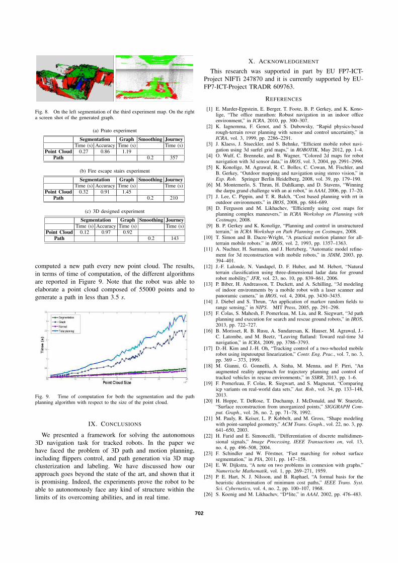
Fig. 8. On the left segmentation of the third experiment map. On the righta screen shot of the generated graph.
(a) Prato experiment
Segmentation Graph Smoothing JourneyTime (s) Accuracy Time (s) Time (s)
Point Cloud 0.27 0.86 1.19Path 0.2 357
(b) Fire escape stairs experiment
Segmentation Graph Smoothing JourneyTime (s) Accuracy Time (s) Time (s)
Point Cloud 0.32 0.91 1.45Path 0.2 210
(c) 3D designed experiment
Segmentation Graph Smoothing JourneyTime (s) Accuracy Time (s) Time (s)
Point Cloud 0.12 0.97 0.92Path 0.2 143
computed a new path every new point cloud. The results,in terms of time of computation, of the different algorithmsare reported in Figure 9. Note that the robot was able toelaborate a point cloud composed of 55000 points and togenerate a path in less than 3.5 s.
Fig. 9. Time of computation for both the segmentation and the pathplanning algorithm with respect to the size of the point cloud.
IX. CONCLUSIONS
We presented a framework for solving the autonomous3D navigation task for tracked robots. In the paper wehave faced the problem of 3D path and motion planning,including flippers control, and path generation via 3D mapclusterization and labeling. We have discussed how ourapproach goes beyond the state of the art, and shown that itis promising. Indeed, the experiments prove the robot to beable to autonomously face any kind of structure within thelimits of its overcoming abilities, and in real time.
X. ACKNOWLEDGEMENT
This research was supported in part by EU FP7-ICT-Project NIFTi 247870 and it is currently supported by EU-FP7-ICT-Project TRADR 609763.
REFERENCES
[1] E. Marder-Eppstein, E. Berger, T. Foote, B. P. Gerkey, and K. Kono-lige, “The office marathon: Robust navigation in an indoor officeenvironment,” in ICRA, 2010, pp. 300–307.
[2] K. Iagnemma, F. Genot, and S. Dubowsky, “Rapid physics-basedrough-terrain rover planning with sensor and control uncertainty,” inICRA, vol. 3, 1999, pp. 2286–2291.
[3] J. Klaess, J. Stueckler, and S. Behnke, “Efficient mobile robot navi-gation using 3d surfel grid maps,” in ROBOTIK, May 2012, pp. 1–4.
[4] O. Wulf, C. Brenneke, and B. Wagner, “Colored 2d maps for robotnavigation with 3d sensor data,” in IROS, vol. 3, 2004, pp. 2991–2996.
[5] K. Konolige, M. Agrawal, R. C. Bolles, C. Cowan, M. Fischler, andB. Gerkey, “Outdoor mapping and navigation using stereo vision,” inExp. Rob. Springer Berlin Heidelberg, 2008, vol. 39, pp. 179–190.
[6] M. Montemerlo, S. Thrun, H. Dahlkamp, and D. Stavens, “Winningthe darpa grand challenge with an ai robot,” in AAAI, 2006, pp. 17–20.
[7] J. Lee, C. Pippin, and T. R. Balch, “Cost based planning with rrt inoutdoor environments.” in IROS, 2008, pp. 684–689.
[8] D. Ferguson and M. Likhachev, “Efficiently using cost maps forplanning complex maneuvers,” in ICRA Workshop on Planning withCostmaps, 2008.
[9] B. P. Gerkey and K. Konolige, “Planning and control in unstructuredterrain,” in ICRA Workshop on Path Planning on Costmaps, 2008.
[10] T. Simon and B. Dacre-Wright, “A practical motion planner for all-terrain mobile robots.” in IROS, vol. 2, 1993, pp. 1357–1363.
[11] A. Nuchter, H. Surmann, and J. Hertzberg, “Automatic model refine-ment for 3d reconstruction with mobile robots,” in 3DIM, 2003, pp.394–401.
[12] J.-F. Lalonde, N. Vandapel, D. F. Huber, and M. Hebert, “Naturalterrain classification using three-dimensional ladar data for groundrobot mobility,” JFR, vol. 23, no. 10, pp. 839–861, 2006.
[13] P. Biber, H. Andreasson, T. Duckett, and A. Schilling, “3d modelingof indoor environments by a mobile robot with a laser scanner andpanoramic camera,” in IROS, vol. 4, 2004, pp. 3430–3435.
[14] J. Diebel and S. Thrun, “An application of markov random fields torange sensing,” in NIPS. MIT Press, 2005, pp. 291–298.
[15] F. Colas, S. Mahesh, F. Pomerleau, M. Liu, and R. Siegwart, “3d pathplanning and execution for search and rescue ground robots,” in IROS,2013, pp. 722–727.
[16] B. Morisset, R. B. Rusu, A. Sundaresan, K. Hauser, M. Agrawal, J.-C. Latombe, and M. Beetz, “Leaving flatland: Toward real-time 3dnavigation,” in ICRA, 2009, pp. 3786–3793.
[17] D.-H. Kim and J.-H. Oh, “Tracking control of a two-wheeled mobilerobot using inputoutput linearization,” Contr. Eng. Prac., vol. 7, no. 3,pp. 369 – 373, 1999.
[18] M. Gianni, G. Gonnelli, A. Sinha, M. Menna, and F. Pirri, “Anaugmented reality approach for trajectory planning and control oftracked vehicles in rescue environments,” in SSRR, 2013, pp. 1–6.
[19] F. Pomerleau, F. Colas, R. Siegwart, and S. Magnenat, “Comparingicp variants on real-world data sets,” Aut. Rob., vol. 34, pp. 133–148,2013.
[20] H. Hoppe, T. DeRose, T. Duchamp, J. McDonald, and W. Stuetzle,“Surface reconstruction from unorganized points,” SIGGRAPH Com-put. Graph., vol. 26, no. 2, pp. 71–78, 1992.
[21] M. Pauly, R. Keiser, L. P. Kobbelt, and M. Gross, “Shape modelingwith point-sampled geometry,” ACM Trans. Graph., vol. 22, no. 3, pp.641–650, 2003.
[22] H. Farid and E. Simoncelli, “Differentiation of discrete multidimen-sional signals,” Image Processing, IEEE Transactions on, vol. 13,no. 4, pp. 496–508, 2004.
[23] F. Schindler and W. Forstner, “Fast marching for robust surfacesegmentation,” in PIA, 2011, pp. 147–158.
[24] E. W. Dijkstra, “A note on two problems in connexion with graphs,”Numerische Mathematik, vol. 1, pp. 269–271, 1959.
[25] P. E. Hart, N. J. Nilsson, and B. Raphael, “A formal basis for theheuristic determination of minimum cost paths,” IEEE Trans. Syst.Sci. Cybernetics, vol. 4, no. 2, pp. 100–107, 1968.
[26] S. Koenig and M. Likhachev, “D*lite,” in AAAI, 2002, pp. 476–483.
702

Point Cloud Segmentation and 3D Path Planning for Tracked Vehiclesin Cluttered and Dynamic Environments
Federico Ferri and Mario Gianni and Matteo Menna and Fiora PirriALCOR, Vision, Perception and Cognitive Robotics Laboratory
DIAG, University of Rome ‘Sapienza‘, Italy{ferri, gianni, menna, pirri}@dis.uniroma1.it
Abstract— The paper presents a framework for tracked ve-hicle 3D path planning in rough areas, with dynamic obstacles.The framework provides methods for real-time point cloudinterpretation, segmentation and traversabilty analysis tackingalso into account changes such as dynamic obstacles andprovides a terrain structure interpretation. Moreover the paperpresents R2A? an extended version of randomized A? copingwith difficult terrains and complex paths for non-holonomicrobots.
I. INTRODUCTION
Navigation in urban disaster environments is a challengingtask. Though tracked robots (UGV) are well equipped tooperate in clutter, search and rescue operations still requirea human operator to remotely teleoperate the robot [1], [2].That is why improving autonomy for these robots is a pivotalissue in search and rescue. To this end, terrain structureinterpretation is a fundamental precondition to move towardautonomy or semi-autonomy and it is still an open problem.Indeed, to guarantee safe autonomous UGV navigation bothpath planning and trajectory tracking controllers requirereal-time interpretation of off-road heterogeneous harsh andcomplex outdoor terrains. The development of effective andaccurate three dimensional maps provides, in fact, a goodground for 3D path planning.
An overview on terrain traversabilty methods can befound in [3]. Most of the methods use geometric featuresto interpret the terrain. For example, in [4], the authorsuse normal vector estimation from stereo vision to estimateinclination of a sector in an elevation map. In [5] the 3D pathplanning algorithm requires an initialization step to builda geometrical representation of the environment, from laserdata. As the map of the environment changes, this step hasto be re-iterated. Therefore, the approach does not seem tobe appropriate for exploration missions, where map updatesoccur frequently. Moreover the approach works only in staticenvironments.
In this work we propose a framework to deal with dynamic3D environment mapping. We provide a general method toreal-time point cloud interpretation, segmentation and affor-dance of the full 3D environments, managing changes, suchas dynamic obstacles. Our approach differs from probabilisticones [6], [7] needing multiple observations for a completeupdate of dynamic obstacles, as it relies on a compactrepresentation, requiring to store just obstacle points withnormal information, in so allowing to recover information
about free space. The approach provides a terrain structureinterpretation, via terrain transferability analysis, and intro-duces a path planner formalization based on randomizedA?. The remainder of this paper is organized as follows.Section II describes the overall framework, introducing somenotation too. Section III introduces the dynamic obstaclesremoval method. Section IV proposes the basic ideas forcomputing geometric features addressing both light andaccurate segmentation. The terrain analysis is presented inSection V and the path planner is described in Section VI. Weconclude with the description of the experiments performedto evaluate the proposed method in Section VII and someinsight for future work is addressed in Section VIII.
II. FRAMEWORK OVERVIEW
An overview of the framework is resumed in Figure 1.The framework is composed of two different pipelines. Thefirst pipeline, shown at the bottom of Figure 1, comprisesthe computational steps needed for a global path planner togenerate long distance paths toward the goal. The secondone, shown at the top of Figure 1, illustrates the sequence ofsteps to compute local paths toward intermediate sub-goals,as described in Section VI.
The first pipeline has been designed with the main purposeof providing a fast and approximated interpretation of theenvironment, where a global planning can take place. Inparallel the second pipeline has the main role of locallybuild a more accurate model of the environment, neededfor traversability assessment and local path planning. TheScant , acquired from the rolling laser sensor of the robot attime t, is filtered for outliers removal and registered via aniterative closest point (ICP) algorithm [8]. The accumulatedmap of the environment Mapt , at time t, is clustered andlabeled using both normals and surface variation features,estimated at large neighborhoods (see Section IV). Theglobal path planner takes as input the goal position qGand the labeled map LMapt , returned by the segmentationprocess, and it provides the local 3D path planner, giving apreliminary information on the goal reachability. For pointsin Scant , which are close to the robot current position, boththe normals and the principals curvatures k1 and k2 areestimated, providing an accurate classification for curvature.The labeled SScant is further merged with the accumulatedsegmented map SMapt−1, at time t−1. This process requiresthe following two steps: (1) removal of dynamic obstacles,
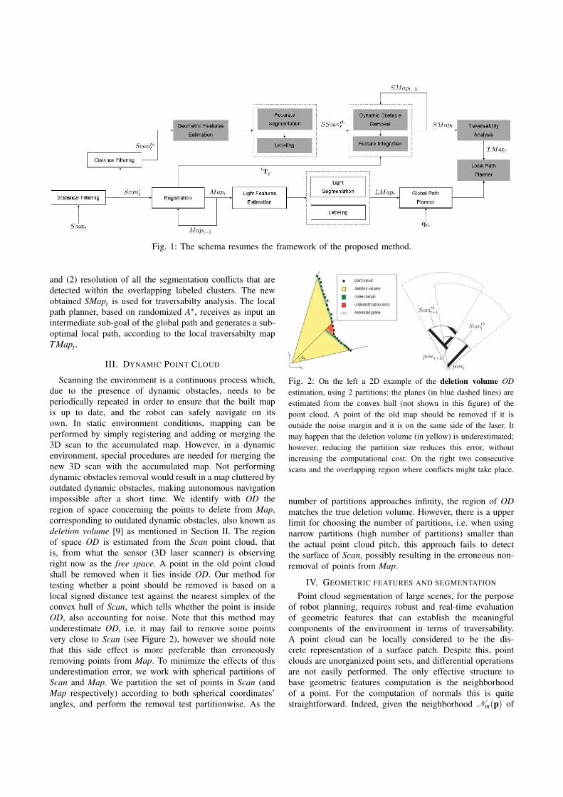
Fig. 1: The schema resumes the framework of the proposed method.
and (2) resolution of all the segmentation conflicts that aredetected within the overlapping labeled clusters. The newobtained SMapt is used for traversabilty analysis. The localpath planner, based on randomized A?, receives as input anintermediate sub-goal of the global path and generates a sub-optimal local path, according to the local traversabilty mapT Mapt .
III. DYNAMIC POINT CLOUD
Scanning the environment is a continuous process which,due to the presence of dynamic obstacles, needs to beperiodically repeated in order to ensure that the built mapis up to date, and the robot can safely navigate on itsown. In static environment conditions, mapping can beperformed by simply registering and adding or merging the3D scan to the accumulated map. However, in a dynamicenvironment, special procedures are needed for merging thenew 3D scan with the accumulated map. Not performingdynamic obstacles removal would result in a map cluttered byoutdated dynamic obstacles, making autonomous navigationimpossible after a short time. We identify with OD theregion of space concerning the points to delete from Map,corresponding to outdated dynamic obstacles, also known asdeletion volume [9] as mentioned in Section II. The regionof space OD is estimated from the Scan point cloud, thatis, from what the sensor (3D laser scanner) is observingright now as the free space. A point in the old point cloudshall be removed when it lies inside OD. Our method fortesting whether a point should be removed is based on alocal signed distance test against the nearest simplex of theconvex hull of Scan, which tells whether the point is insideOD, also accounting for noise. Note that this method mayunderestimate OD, i.e. it may fail to remove some pointsvery close to Scan (see Figure 2), however we should notethat this side effect is more preferable than erroneouslyremoving points from Map. To minimize the effects of thisunderestimation error, we work with spherical partitions ofScan and Map. We partition the set of points in Scan (andMap respectively) according to both spherical coordinates’angles, and perform the removal test partitionwise. As the
Fig. 2: On the left a 2D example of the deletion volume ODestimation, using 2 partitions: the planes (in blue dashed lines) areestimated from the convex hull (not shown in this figure) of thepoint cloud. A point of the old map should be removed if it isoutside the noise margin and it is on the same side of the laser. Itmay happen that the deletion volume (in yellow) is underestimated;however, reducing the partition size reduces this error, withoutincreasing the computational cost. On the right two consecutivescans and the overlapping region where conflicts might take place.
number of partitions approaches infinity, the region of ODmatches the true deletion volume. However, there is a upperlimit for choosing the number of partitions, i.e. when usingnarrow partitions (high number of partitions) smaller thanthe actual point cloud pitch, this approach fails to detectthe surface of Scan, possibly resulting in the erroneous non-removal of points from Map.
IV. GEOMETRIC FEATURES AND SEGMENTATION
Point cloud segmentation of large scenes, for the purposeof robot planning, requires robust and real-time evaluationof geometric features that can establish the meaningfulcomponents of the environment in terms of traversability.A point cloud can be locally considered to be the dis-crete representation of a surface patch. Despite this, pointclouds are unorganized point sets, and differential operationsare not easily performed. The only effective structure tobase geometric features computation is the neighborhoodof a point. For the computation of normals this is quitestraightforward. Indeed, given the neighborhood Nm(p) of
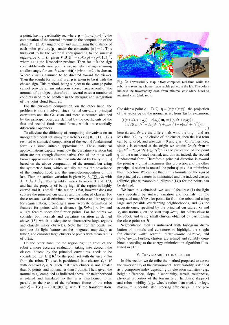
a point, having cardinality m, where p = (x,y,z(x,y))>, thecomputation of the normal amounts to the computation of theplane π = (n,d) tangent to p, and minimizing the distance ofeach point pi ∈Nm(p), under the constraint ‖n‖ = 1. Thisturns out to be the vector u corresponding to the smallesteigenvalue λ in D, given V D U> = (Nm(p)− (p⊗1m))
>,where ⊗ is the Kronecker product. Then for ±u the signcompatible with view point view, namely the sign ensuringsmallest angle for cos−1(view−±u)/‖view−±u‖, is chosen.Where view is assumed to be directed toward the viewer.Then the sought for normal n at p is taken to be u with thechosen sign. This method, being subject to the vantage pointcannot provide an instantaneous correct assessment of thenormals of an object, therefore in several cases a number ofconflicts need to be handled in the merging and integrationof the point cloud features.
For the curvature computation, on the other hand, theproblem is more involved, since normal curvature, principalcurvatures and the Gaussian and mean curvatures obtainedby the principal ones, are defined by the coefficients of thefirst and second fundamental forms, which are essentiallydifferential operators.
To alleviate the difficulty of computing derivatives on anunorganized point set, many researchers (see [10], [11], [12])resorted to statistical computation of the second fundamentalform, via some suitable approximation. These statisticalapproximations capture somehow the curvature variation butoften are not enough discriminative. One of the most wellknown approximation is the one introduced by Pauly in [13]based on the above computation of the normal, but usingthe symmetric form, which actually returns the covarianceof the neighborhood, and the eigen-decomposition of thislast. Then the surface variation is given by λ1/∑3
i=1 λi withλ1 ≤ λ2 ≤ λ3. This quantity varies between 0 and 1/3,and has the property of being high if the region is highlycurved and it is small if the region is flat, however does notcapture the principal curvatures and the induced classes. Forthese reasons we discriminate between close and far regionsfor segmentation, providing a more accurate estimation offeatures for points with a distance ‖p,Robot‖ < 3m anda light feature space for further points. For far points weconsider both normals and curvature variation as definedabove [13], which is adequate to characterize large regionsand classify major obstacles. Note that for far points wecompute the light features on the integrated map Mapt attime t, and consider large clusters of points with mean radiusof 0.2m.
On the other hand for the region right in front of therobot a more accurate evaluation, taking into account theclasses induced by the principal curvatures, needs to beconsidered. Let H ∈R3 be the point set with distance < 3mfrom the robot. This set is partitioned into clusters Ci ⊂ Hwith centroid ci ∈ H, such that each cluster is not greaterthan 50 points, and not smaller than 7 points. Then, given thenormal to ci, computed as indicated above, the neighborhoodis rotated and translated so that n is transformed to nzparallel to the z-axis of the reference frame of the robotand c′i = T(ci) = (0,0,z(0,0)), with T the transformation.
Fig. 3: Traversability map T Map computed real-time while therobot is traversing a home-made rubble pallet, in the lab. The colorsindicate the traversabilty cost, from minimal cost (dark blue) tomaximal cost (dark red).
Consider a point q ∈ T(C), q = (x,y,z(x,y)), the projectionof the vector cq on the normal nz is, from Taylor expansion:
(z(x+dx,y+dy)− z(x,y))nz = ((zxdx+ zydy)+(1/2)(zxxdx2 +2zxydxdy+ zyydy2)+o(dx2 +dy2)
)nz
(1)here dx and dy are the differentials w.r.t. the origin and areless than 0.2, by the choice of the cluster, then the last termcan be ignored, and also zxn = 0 and zyn = 0. Furthermore,since c is centered at the origin we obtain: 2z(dx,dy)n =(zxxdx2 +2zxydxdy+ zyydy2)n as the projection of the pointq on the transformed normal, and this is, indeed, the secondfundamental form. Therefore a principal direction is towardthe point q 6= c that maximizes this projection and the otherprincipal direction is toward the point q′ 6= c that minimizesthis projection. We can see that in this formulation the sign ofthe principal curvatures is maintained and the induced classes(elliptic, planar, paraboloid, ellipsoid[14]) for the points canbe defined.
We have thus obtained two sets of features: (1) the lightones specified by surface variation and normals, on theintegrated map Mapt , for points far from the robot, and usinglarge and possible overlapping neighborhoods, and (2) theaccurate ones, specified by the principal curvatures κ1 andκ2 and normals, on the scan map Scant , for points close tothe robot, and using small clusters obtained by partitioningthe close point set H.
Segmentation then is initialized with histogram distri-bution of normals and curvatures to highlight the soughtfor classes: walls, terrain, surmountable obstacle, andstairs/ramps. Further, clusters are refined and suitably com-bined according to the energy minimization algorithm illus-trated in [15].
V. TRAVERSABILITY IN CLUTTER
In this section we describe the method proposed to assessthe traversability of the environment. Traversability is definedas a composite index depending on elevation statistics (e.g.,height difference, slope, discontinuity, terrain roughness),physical properties of the terrain (e.g., hardness, slippery)and robot mobility (e.g., wheels rather than tracks, or legs,maximum superable step, steering efficiency). In the pro-

posed approach traversability is assessed with a cost function,which takes into account the following geometrical featuresof the surrounding environment: (1) terrain roughness; (2)terrain classification, based on both terrain slope and robotlocomotion capabilities; (3) obstacle clearance and (4) pointcloud density. This cost function has been defined as follows.Let SMapt be the segmented point cloud, at time t, introducedin Section IV. Let p ∈ SMapt a point of the point cloud.The point-wise traversability cost function f : SMap 7→ R,returning the static traversability cost of the point p∈ SMapt ,is given by
f (p) := w(p)L ·
(w(p)
CL +w(p)Dens +w(p)
Rough
)(2)
Here the term w(p)L represents the contribution to the overall
cost of p ∈ SMapt , computed according to the segmentationof the local map. This cost term is lower for points belongingto clusters labeled as ground, while increases for pointsbelonging to clusters, which are more difficult to traverse,such as those labeled with stairs or ramps. w(p)
CL is thecost contribution provided by the obstacle clearance. Pointsbelonging to clusters which are relatively close to obstacles,inflated by the inscribed radius of the robot, have beenassigned with a higher cost, since they are unreachable forthe robot. This cost term is computed as follows
w(p)CL =
1max{min{||p−p′||} ,∆}−∆
(3)
for all p′ ∈ SMapt , such that p′ belongs to clusters labeledeither as wall or ceiling. Here ∆ is the inflated radius (seeFigure 4). Note that this approach is similar to the artificialpotential fields methodology, proposed in [16]. w(p)
Dens rep-resents the contribution to the overall cost of p ∈ SMapt ,computed with respect to the point cloud density, as follows
w(p)Dens =
|Nr(p)|43 πr3
(4)
Here |Nr(p)| is the cardinality of the set of points belongingto the neighborhood of p ∈ SMapt . High values of w(p)
Dens areassigned to points p ∈ SMapt which are relatively close toterrain regions not correctly segmented, due to unevennessof the terrain, holes or lack of laser scan data. This cost termhas the effect of deterring navigation near such areas. w(p)
Roughmeasures the terrain roughness. Roughness is estimated bycomputing the average distance of the outliers from the planefitted on the points belonging to the neighborhood Nr(p)of p ∈ SMapt . By applying the defined traversability costfunction f (p), ∀p ∈ SMapt , we obtain the traversability mapT Mapt of the environment.
VI. PATH PLANNER
The global path planer, which we do not discuss here,computes a main direction toward a goal, either given orgenerated. The local path planner computes the interme-diate steps toward this goal. In this section we presentthe local path planner based on randomized A? (RA?) [17]and extended to cope with non-holonomic robots and largepoint clouds. Similarly to RA? the proposed algorithm R2A?
Δ
pos(v)
wCL
Fig. 4: On the left a plot of the term wCL as a function of thevertex position. The dashed region represents an obstacle, and thecontinuous blue line is the cost. On the right the boundary of apoint neighborhood, with highlighted the two sets Q1 and Q2.
samples the action space, uses a k-dimensional tree datastructure for partitioning and adapts the branching factoraccording to a search radius. Differently from RA? wepropose a density function acting on the boundary of thecurrent location neighborhood.
Let qLG be an intermediate goal, that is, a position inthe traversability map T Mapt at a distance less than a giventhreshold. If there exists a path from the current robotposition to qLG, the local path planner computes it. The basicidea of the proposed algorithm is to generate a search treeG = 〈N,E〉, N the set of nodes and E the set of the edges,by sampling candidate poses. Sampling is governed by aprobability density function defined on the traversabilty mapT Mapt , at time t. The novelty of the approach is to reducethe search space still ensuring to find a path if this exists.
We first introduce some notation. A path path is anordered list of nodes, such that if two adjacent nodes ni,ni+1are in path then there exists an edge directly linking them,where an edge E between two nodes is a relation definedaccording to the robot length. A trajectory τ is a curvespecified by arc length s, s ∈ [0,1] and it is defined on thetraversability map.
The function pos : N→ R3 returns the coordinates of thepoint p∈ T Mapt , associated with the node n∈N, the functionparent : N → R returns the coordinates of the point p′ ∈T Mapt , associated to the parent of a node n ∈ N. We denotevisited the data structure storing the visited nodes and denoteleaf the data structure storing the current leaf nodes, namely,the frontier of the search tree G .
Given a point p∈ T Mapt such that p= pos(n), with n∈N,the neighborhood of p is denoted Nr(p), as in Section IV,where here r denotes the radius of the neighborhood; andwith ∂Nr we denote the boundary of the neighborhood,namely ∂Nr(p) = {p′ ∈ Nr|‖ p− p′‖ − r < ε}. Finally,the density for p ∈ T Mapt is g f = α(1/ f (p)), where f isdefined in eq. (2) and α = ∑m
1 (1/ f (pi)),pi ∈ Nr(p) is anormalization term, m the cardinality of the neighborhoodof p. The density reinforces points with low traversabilitycost.
The parameters of a node are the followings:• The euclidean distance d : R3×R3 → R between the
position of two nodes.• The set Q1,n = {p ∈ R3|p = λp+(1−λ )p′}, with λ ∈[0,1], p′ = pos(n) and p = parent(n).

• The set Q2,n = {p∈ T Mapt |d(p, p)< ρ}, ∀p∈Q1, withρ half the robot length. See Figure 4.
• The traversability cost f (pos(n)), defined in eq. (2).• The cost f ′ : R3 → R defined as f ′(n) = max{ f (p)},∀p ∈ Q2,n.
• The admissible goal heuristic h? :R3×R3→R, betweenthe position of the current node and the goal node.
• The function r : R3→ R, which sets the search radius,finding the distance of a point p ∈ T Mapt from thenearest obstacle, defined as follows:
r(pos(n)) = minp′∈T Mapt
{∥∥pos(n)−p′∥∥
2
}(5)
∀p.p ∈ T Map′t with p belonging to clusters labeledeither as wall or ceiling.
The generation and expansion of the tree G is definedinductively as follows. For the basic step, the initial noden0 = pos(probot), namely the current robot position, is in N.
For the induction step. Let n ∈ N and consider the datastructures visited and lea f .
Generation Candidate nodes are sampled according to thedensity g f . A node n? is chosen among the set of candidatenodes if the following two conditions are satisfied.
1) n? /∈ visited;2) ∃p ∈ T Mapt such that p ∈ Q1,n? , with p = parent(n?)
If n? satisfies the above conditions then it is added to theleaf data structure.
Expansion Given a node n ∈ lea f , the node is expandedaccording to the above parameters, used in the followingrules. Let us assign to each p ∈ ∂Nr(pos(n)) the valueg f (p) =α 1
f (p) , where the radius r defining the neighborhoodhas been computed as in eq. (5). Here, we are implicitlydefining a discrete probability distribution over ∂Nr(pos(n))in which points with lower traversability cost have highprobability.
In principle we are computing a continuous trajectory τ(s),between n0 and nG, where s ∈ [0,1], and with the cost of thetrajectory within the traversability map defined as:
∫ 1
0costT Map(τ(s))ds (6)
Since R2A? returns a discrete path we approximate thiscontinuous cost with the following cost function defined foreach node:
cost(n)= f ′(pos(n))+d(pos(n), parent(n))+h?(pos(n),qLG)
And, thus, the approximated trajectory cost is the cost of theexpanded nodes, obtained by minimizing:
∑i
cost(n)i, ∀ni ∈ path (7)
The algorithm starts to expand the node in leaf with theminimum cost and ends as soon as the current neighborhoodis the one of the goal node, and the distance to the goal nodeis less than the robot size.
We show, now, that if there exists an admissible pathbetween two points which is found by A? then there is a pathcomputed by the proposed algorithm R2A?. More precisely,
Fig. 5: On the left a person is standing in front of a wall (dark blueblob on the left). The white blob behind the person indicates that thepoint cloud of the region of the wall has not been aggregated intothe entire map of the area, due to occlusion. On the right the resultof the dynamic correction algorithm: after the motion of the person,the map is updated by both deleting the blob of the person and byaggregating the point cloud of the region of the wall, previouslyoccluded.
let n0 denote the start node and nG the goal node and assumethat A? computes the path Q such that n0,nG ∈ Q then:
Lemma 1: There exists a path path computedby R2A? such that n0,nG ∈ path and ∑i cost(n)i ≤∑i d(parent(ni), pos(ni))+wih?(ni,nG).Proof. First note that we have made explicit a penalty wiadded to h? to balance the lack of the traversability cost termin the A? cost function. Now, observe that in Q there mustexists a node nb that belongs to ∂N (n0) since any path fromn0 to nG has to pass from the boundary of the neighborhoodof n0. Therefore the proof can be done by induction onthe number of boundaries traversed. As basic step, assumenG belongs to the neighborhood of n0 and is not on theboundary, this implies there are no obstacles and thus A?
and R2A? coincide finding a straight trajectory. Assume, now,that the current node is n, with ∂N (pos(n)) the boundaryof its neighborhood, and there exists a path from n to nG,then there exists a node nb with pos(nb) ∈ ∂N (n) such thatcost(nb)+ cost(nG)≤ cost(n)+ cost(nG). In fact R2A? findsthe boundary node before A? because of the condition of theexpansion. Clearly also A? must sooner or later pass throughthe boundary, but since it does not overestimate the cost andchooses straight lines, in the worst case it might cross theboundary after having expanded a greater number of nodesthan R2A?, hence the path cost must be greater. �
We have thus shown that R2A? behaves like A? in the worstcase and also that its cost cannot exceed A?. The proof thatits cost is admissible is here omitted.
R2A? nodes in a path over 6 runsA? run1 run2 run3 run4 run5 run6138 72 69 75 81 71 87
TABLE I
VII. EXPERIMENTS
We evaluated the framework on the dynamic point cloudand on the 3D path planner, also comparing R2A? and A?
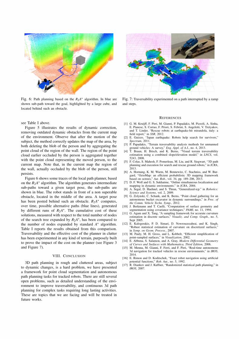
Fig. 6: Path planning based on the R2A? algorithm. In blue areshown sub-path toward the goal, highlighted by a large cube, andlocated behind such an obstacle.
see Table I above.Figure 5 illustrates the results of dynamic correction,
removing outdated dynamic obstacles from the current mapof the environment. Observe that after the motion of thesubject, the method correctly updates the map of the area, byboth deleting the blob of the person and by aggregating thepoint cloud of the region of the wall. The region of the pointcloud earlier occluded by the person is aggregated togetherwith the point cloud representing the moved person, to thecurrent map. Note that, in the current map the region ofthe wall, actually occluded by the blob of the person, stillpersists.
Figure 6 shows some traces of the local path planner, basedon the R2A? algorithm. The algorithm generates intermediatesub-paths toward a given target pose, the sub-paths areshown in blue. The robot stands in front of a non superableobstacle, located in the middle of the area. A target posehas been posted behind such an obstacle. R2A? computes,over time, possible alternative paths (blue lines), generatedby different runs of R2A?. The cumulative cost of thesesolutions, measured with respect to the total number of nodesof the search tree expanded by R2A?, has been compared tothe number of nodes expanded by standard A? algorithm.Table I reports the results obtained from this comparison.Traversability and the effective cost of the planner in clutterhas been experimented in any kind of terrain, purposely builtto prove the impact of the cost on the planner (see Figure 3and Figure 7).
VIII. CONCLUSION
3D path planning in rough and cluttered areas, subjectto dynamic changes, is a hard problem, we have presenteda framework for point cloud segmentation and autonomouspath planning tasks for tracked robots. There are still severalopen problems, such as detailed understanding of the envi-ronment to improve traversability, and continuous 3d pathplanning for complex tasks requiring long lasting activities.These are topics that we are facing and will be treated infuture works.
Fig. 7: Traversability experimented on a path interrupted by a rampand steps.
REFERENCES
[1] G. M. Kruijff, F. Pirri, M. Gianni, P. Papadakis, M. Pizzoli, A. Sinha,E. Pianese, S. Corrao, F. Priori, S. Febrini, S. Angeletti, V. Tretyakov,and T. Linder, “Rescue robots at earthquake-hit mirandola, italy: afield report,” in SSR, 2012.
[2] E. Guizzo, “Japan earthquake: Robots help search for survivors,”Spectrum, 2011.
[3] P. Papadakis, “Terrain traversability analysis methods for unmannedground vehicles: A survey,” Eng. Appl. of A.I., no. 4, 2013.
[4] T. Braun, H. Bitsch, and K. Berns, “Visual terrain traversabilityestimation using a combined slope/elevation model.” in LNCS, vol.5243, 2008.
[5] F. Colas, S. Mahesh, F. Pomerleau, M. Liu, and R. Siegwart, “3D pathplanning and execution for search and rescue ground robots,” in ICRA,2013.
[6] A. Hornung, K. M. Wurm, M. Bennewitz, C. Stachniss, and W. Bur-gard, “OctoMap: an efficient probabilistic 3D mapping frameworkbased on octrees,” Aut. Rob., vol. 34, pp. 189–206, 2013.
[7] D. F. Wolf and G. S. Sukhatme, “Online simultaneous localization andmapping in dynamic environments.” in ICRA, 2004.
[8] A. Segal, D. Haehnel, and S. Thrun, “Generalized-icp.” in Robotics:Science and Systems, vol. 2, 2009.
[9] G. Zolynski, C. Schank, and K. Berns, “Point cloud gathering for anautonomous bucket excavator in dynamic surroundings,” in Proc. ofthe Comm. Vehicle Techn. Symp., 2012.
[10] J. Berkmann and T. Caelli, “Computation of surface geometry andsegmentation using covariance techniques,” PAMI, no. 11, 1994.
[11] G. Agam and X. Tang, “A sampling framework for accurate curvatureestimation in discrete surfaces,” Visualiz. and Comp. Graph., no. 5,Sept 2005.
[12] E. Kalogerakis, P. D. Simari, D. Nowrouzezahrai, and K. Singh,“Robust statistical estimation of curvature on discretized surfaces,”in Symp. on Geom. Process., 2007.
[13] M. Pauly, M. H. Gross, and L. Kobbelt, “Efficient simplification ofpoint-sampled surfaces,” in Visualization, 2002.
[14] E. Abbena, S. Salamon, and A. Gray, Modern Differential Geometryof Curves and Surfaces with Mathematica, Third Edition, 2006.
[15] M. Menna, M. Gianni, F. Ferri, and F. Pirri, “Real-time autonomous3d navigation for tracked vehicles in rescue environments,” in IROS,2014.
[16] E. Rimon and D. Koditschek, “Exact robot navigation using artificialpotential functions,” Rob. Aut., no. 5, 1992.
[17] R. Diankov and J. Kuffner, “Randomized statistical path planning,” inIROS, 2007.

21
A Stimulus-Response Framework for Robot Control
MARIO GIANNI, ALCOR Laboratory, DIIAG, Sapienza, University of Rome, ItalyGEERT-JAN M. KRUIJFF, Nuance Deutschland GmbH, Aachen, GermanyFIORA PIRRI, ALCOR Laboratory, DIIAG, Sapienza, University of Rome, Italy
We propose in this article a new approach to robot cognitive control based on a stimulus-response frameworkthat models both a robot’s stimuli and the robot’s decision to switch tasks in response to or inhibit the stimuli.In an autonomous system, we expect a robot to be able to deal with the whole system of stimuli and to usethem to regulate its behavior in real-world applications. The proposed framework contributes to the stateof the art of robot planning and high-level control in that it provides a novel perspective on the interactionbetween robot and environment. Our approach is inspired by Gibson’s constructive view of the concept ofa stimulus and by the cognitive control paradigm of task switching. We model the robot’s response to astimulus in three stages. We start by defining the stimuli as perceptual functions yielded by the active robotprocesses and learned via an informed logistic regression. Then we model the stimulus-response relationshipby estimating a score matrix that leads to the selection of a single response task for each stimulus, basingthe estimation on low-rank matrix factorization. The decision about switching takes into account both aninterference cost and a reconfiguration cost. The interference cost weighs the effort of discontinuing thecurrent robot mental state to switch to a new state, whereas the reconfiguration cost weighs the effort ofactivating the response task. A choice is finally made based on the payoff of switching. Because processes playsuch a crucial role both in the stimulus model and in the stimulus-response model, and because processes areactivated by actions, we address also the process model, which is built on a theory of action. The framework isvalidated by several experiments that exploit a full implementation on an advanced robotic platform and iscompared with two known approaches to replanning. Results demonstrate the practical value of the systemin terms of robot autonomy, flexibility, and usability.
Categories and Subject Descriptors: I.2.9 [Robotics]: Autonomous Vehicles, Operator Interfaces; I.2.10[Vision and Scene Understanding]: Perceptual Reasoning, Representations, Data structures, and Trans-forms; F.4.1 [Mathematical Logic]: Logic and Constraint Programming; I.2.4 [Knowledge Representa-tion Formalisms and Methods]: Predicate Logic, Situation Calculus, Relation System, RepresentationLanguages; I.2.6 [Learning]: Parameter Learning, Induction; I.2.8 [Problem Solving, Control Methods,Search]: Plan Execution, Formation, and Generation
General Terms: Design, Algorithms, Performance, Reliability, Languages
Additional Key Words and Phrases: Task switching, intelligent interaction, stimulus-response model, behav-ior adaptation
ACM Reference Format:Mario Gianni, Geert-Jan M. Kruijff, and Fiora Pirri. 2015. A stimulus-response framework for robot control.ACM Trans. Interact. Intell. Syst. 4, 4, Article 21 (January 2015), 41 pages.DOI: http://dx.doi.org/10.1145/2677198
This work is supported by the EU-FP7 ICT 247870 NIFTI project.The reviewing of this article was managed by Lutz Frommberger, Heriberto Cuayahuitl, Nina Dethlefs,Antoine Raux, Matthew Marge, and Hendrik Zender.Authors’ addresses: M. Gianni and F. Pirri, ALCOR LAB, Dipartimento di Ingegneria Informatica, Auto-matica e Gestionale, “Antonio Ruberti”, via Ariosto 25, 00185, Roma; emails: {Mario.Gianni, Fiora.Pirri}@dis.uniroma1.it; G.-T. M. Kruijff, Nuance Communications Deutschland GmbH, Kackertstrasse 10, D-52072Aachen, Germany; email: [email protected] to make digital or hard copies of part or all of this work for personal or classroom use is grantedwithout fee provided that copies are not made or distributed for profit or commercial advantage and thatcopies bear this notice and the full citation on the first page. Copyrights for components of this work ownedby others than ACM must be honored. Abstracting with credit is permitted. To copy otherwise, or republish,to post on servers, or to redistribute to lists, requires prior specific permission and/or a fee. Requestedpermissions from [email protected] Copyright is held by the owner/author(s). Publication rights licensed to ACM.ACM 2160-6455/2015/01-ART21 $15.00DOI: http://dx.doi.org/10.1145/2677198
ACM Transactions on Interactive Intelligent Systems, Vol. 4, No. 4, Article 21, Publication date: January 2015.

21:2 M. Gianni et al.
1. INTRODUCTION AND MOTIVATIONS
A robot interacting with people and with the environment is subject to several stimulusevents, like any living organism. How these stimuli are to be represented and how aresponse should be modeled has not yet received the necessary attention, even thoughrobot autonomy, beyond laboratory experiments, relies on an intelligent response tothese stimuli.
Everyone knows what a stimulus is in the human and animal sense. The concept ofstimulus has been studied the eighteenth century, with the work of Galvani and Voltaon frogs, and was further explored in psychology, physiology, and psychophysics. Mod-ern physiology considers a stimulus applied to a receptor and capturing informationfrom both inside and outside the body; these are called proximal and distal stimuli, re-spectively. Following the pioneering work of Weber [1834], Gustav Fechner introducedpsychophysics to model the relation of physical stimuli to the resulting mental facts.Gibson [1960] proposes the following a constructive view of a stimulus:
I think the central question is the following. Is a stimulus that which does activate a sense organ or thatwhich can activate a sense organ? Some writers imply that a stimulus not currently exciting receptorsis not a stimulus at all. Others imply that a stimulus need not excite receptors to be called such. [Gibson1960]
Gibson’s implicit question is about the possibility of giving a structure, a definition, tothe relationship between objects and stimuli and between stimulus and response:
Perhaps there is an invariant stimulus for the invariant response, after all. Many sorts of higher ordervariables of energy may exist, only awaiting mathematical description. They will have to be describedin appropriate terms, of course, not as simple functions of frequency and amount. We must not confusea stimulus with the elements used for its analysis. [Gibson 1960]
As a matter of fact, we do not yet have a model of robot stimuli, and most researchersaccept that any sensory input from the environment or from the robot’s internal statescan be considered a stimulus. This simplification is of no help, as the wide literatureon human and animal stimuli witnesses. If any sensory input can be considered astimulus, how it would be possible for a robot to discern between a wall and a victimlying on the ground, between the light from a fire and the light of a lamp, between ascream and repeated noise, and so on? Not all inputs require a response, but a stimulusdoes.
In this article, we address the problem of providing a representation of what astimulus is for a robot and how it affects the robot’s behavior and its tasks underexecution. Consider that whereas for a living organism pain is a stimulus that has adirect effect on its survival awareness, for a robot, a similar stimulus could be the lack ofa WiFi connection or battery exhaustion, both indicating a loss of vitality. Therefore, inproviding such a representation, we answer the question of how to model the stimulusreflex within the robot’s structure and language, and we explore how the robot learnsthe best stimulus-response according to the context of its current task.
In living organisms, stimulus transduction elicits the stimulus reflex through a re-ceptor. In a robot, this transduction is conveyed by its active processes. Consider therobot motion system, which is made of several components, each of which is driven byprocesses controlling velocity, steering, obstacle avoidance, terrain adaptation, track-ing and so on. These processes collect information from the environment and from therobot’s internal states. These processes elaborate the collected information and updateit, eventually returning it to the robot’s inner states to manage its current activities.In other words, the interaction with environment configures a space of informationallocating to each process a quantum of information that is transduced to a stimulusat specific peaks of the information manifold. A stimulus induces a request with the
ACM Transactions on Interactive Intelligent Systems, Vol. 4, No. 4, Article 21, Publication date: January 2015.

A Stimulus-Response Framework for Robot Control 21:3
call for a response. A response might appeal to robot components and their processesnot yet active at the very moment at which the stimulus is triggered.
In this article, we introduce a preliminary framework to model robot processes,their yields, the stimuli occurrences, and the decision underlying the response to thestimuli. The advantage of this approach is that robot control does not need to bedesigned a priori but instead can be drawn by its interactions with users who teachthe robot when a stimulus occurs and what the possible alternatives are for handlingthe stimuli. These aspects are not dealt with in any other control methods, includingplanning, whether reactive, proactive, or declarative. Indeed, a robot that has learneda stimulus-response strategy from several humans will most certainly be more usablethan a robot that either has no stimuli at all or has no strategy to respond to stimuli.We also take context into account in order to establish a response cost, and we exploita theory of actions that models how tasks are chosen and how switching to a new taskcan occur as a result of a stimulus-response.
The ability to selectively respond to several stimuli and to inhibit inappropriate urgesby focusing on the task at hand are well-known in humans as shifting and inhibitionexecutive functions, respectively [Miller and Cohen 2007; Aron 2007]. The neurosciencetheory of control uses inhibition to explain many cognitive activities, especially toexplain how an individual presented with several stimuli responds selectively and isable to resist inappropriate urges [Tipper 2001].
Since the early work of Jersild [1927], several studies in neuroscience and cognitivescience have led to a better understanding of many of the variables affecting taskswitching in the context of cognitive control (we refer the reader to Monsell [2003]and the citations therein). These theories have strongly influenced cognitive roboticsarchitectures since the 1980s, as, for example the ATA schema [Norman and Shallice1986], the principles of goal-directed behaviors in Newell [1990], and, more recently, theCogX architecture [Hawes et al. 2010; Wyatt et al. 2010]. (For a review on the earliestarchitectures in the framework of the task switching paradigm, see Rubinstein et al.[2001].)
Only recently has the need to model the stimulus-response, and hence the cognitivecontrol underlying task switching and the cognitive functions of shifting and inhibi-tion, become a hot topic in cognitive robotics. The need to model adaptation, to increasethe flexibility in handling complex tasks, has led to modeling task switching for robotnavigation, motion planning, and control in large-scale environments [Althaus andChristensen 2003], for path planning [Medina Ayala et al. 2012], for recognizing hu-man intentions in conversation [Nakano et al. 2011], and for motor planning to improvetasks execution [Ganesh and Burdet 2013]. Task switching is also addressed in manip-ulation [Ajoudani et al. 2013; Ding and Fang 2013] and soft robot control [Tao et al.2012; Li et al. 2013], for modeling multirobot systems [Sung et al. 2013], for learningtask space control through the use of different tools [Jamone et al. 2013], for bipedwalking in rough terrain [Saglam and Byl 2013], and for multiple-space control [Li andCheah 2012].
Most of the cited works are quite recent, showing increasing interest in the stimulus-response framework for coping with adaptivity and ecological behaviors in an inter-active environment. Further examples of these studies exist [Capi 2007; Suzuki et al.2009; Wawerla and Vaughan 2009; Finzi and Pirri 2010; Durkee et al. 2011; D’Ambrosioet al. 2011]. The major problem to be resolved, as noted in Wawerla and Vaughan [2009],is the switching decision. Experts on task switching claim that this decision incurs aswitching cost. This cost results from the interplay between the resources needed toreconfigure a mental state and the resources needed to resolve interference with thecurrent state [Monsell 2003]. We model this cost by considering both the reconfigura-tion of the mental state and the interference with the current state. The reconfiguration
ACM Transactions on Interactive Intelligent Systems, Vol. 4, No. 4, Article 21, Publication date: January 2015.

21:4 M. Gianni et al.
Fig. 1. Work flow of the proposed stimulus-response framework. From bottom to top: the lowest layerindicates a currently active task being executed. The active processes feed the process yields, collectinginformation from them; the stimulus model selects from the yields those which are stimuli. The stimulus-response model scores the response tasks. The decision is taken by evaluating the payoff of switching to a tasksuggested by the stimulus-response matrix. In the middle panel, between knowledge and inference, executionmonitoring takes care of the actual task execution and its updating, both affecting the mental states; namely,the decision of whether to consent to a response to the stimulus. In the upper panel, a first-order logicalformalism is used to model the robot processes, with action preconditions and effects affecting activation costsand motivating causal constraints. This closes the loop between stimulus activation, reasoning, planning,and decision.
and interference costs are defined in terms of the amount of processes that need to beinferred in order to initiate a new task and their congruency with the current task. Thedecision is made based on a payoff that is computed by considering the cost of updatingthe current robot state and the risk of continuing with the task under execution. Thestimulus-response model illustrated in these pages indicates a new direction in robotcognitive control, and the tests and experiments presented here prove that this is apromising direction.
The stimulus-response framework introduces new emerging methodologies thatbuild cognitive robot control via learning and perception, and we expect that it willspread to several applications that require cognitive control to resolve the continuousstruggle a robot has to face in a real-world environment.
2. EXECUTIVE SUMMARY
The flowchart of the proposed robot stimulus-response framework is illustrated inFigure 1. The lower layer represents a robot task under execution. The next levelillustrates the stimuli and the response models, described in Sections 3 and 4. Thelevel enclosed between Inference and Knowledge delineates the work flow linking thedecision level to the current execution level. The upper level provides a schema ofthe system representation in the formal language of Situation Calculus, where themapping of the stream of information into the domain of reasoning takes place. Theselevels are described in Sections 5 and 6.
ACM Transactions on Interactive Intelligent Systems, Vol. 4, No. 4, Article 21, Publication date: January 2015.

A Stimulus-Response Framework for Robot Control 21:5
Table I. Examples of Yields of Processes and Their Features��������Process
Yields and Their Features Stimulus Description
Battery Level Power Consumption Location - ExhaustionWiFi Strength Dist. Source Speed Traffic DisconnectionLaser scan Resolution Surface Density Smoothness Lack of data, device errorMapping Height Slope Intricacy Depth 3D data not available, obstacleVisual perception Shape Dimension Location Distance Identification, DetectionAttention Light Color Motion Contour SaliencyInterface Sound Id Voice Utterance Meaning RequestSound Scale Frequency Pitch Who Mute, Noise
Each active robot process yields a quantum of information with characteristic fea-tures; this quantum of information is called the yield of an active process. The featuresz of the yield are used by the stimulus model to learn a function hβ (z) (Section 3). Thisfunction establishes whether or not a stimulus occurred during the specific processexecution.
Example 2.1. Consider the robot process πWiFi managing the connection betweenthe robot and a remote command base station. We expect that the stimulus occurswhen a high signal becomes low or disappears. So the process πWiFi yields a quantumof information specified by a set of features zWiFi, such as those indicated in Table I.The robot, with the help of users, learns to discriminate a stimulus from ordinaryinformation via the function hβ(zWiFi), discerning between typical zWiFi values andodd ones. Therefore, the outcome of the learned function hβ is a value y = 1 to fire thestimulus of WiFi disconnection and y = 0 otherwise.
If the stimulus occurs, the robot has to choose a possible response (e.g., going back tothe last position where it was connected), or it can inhibit the stimulus and continue itstask even though it is disconnected from the operator. Therefore, there are two issuesthat need to be modeled:
(1) identify the task that is a possible response to the stimulus;(2) decide whether to go on with the current task or to switch to the identified response
task.
The first item is dealt with by filling a score matrix A whose values are estimated viafactorization, as described in Section 4.
On the other hand, the decision to either shift from the current task to a new taskin so responding to the stimulus, or to inhibit the stimulus, is based on the payoff ofswitching. This is computed considering the risk of continuing the current task, withouttaking into account the stimulus, and the effort required to fulfill the stimulus. In turn,the effort is computed considering two costs: (1) the cost to reconfigure the currentrobot state to the new state that switching would lead to and (2) the cost to resolve theinterference due to the interruption of the current task. These costs are computed byconsidering the preconditions and effects of each action involved in both the processesto be interrupted and in the ones to be activated (Section 6). To bind the informationyielded by a process to the domain of reasoning, a special functional E is used, mappingthe process terms of the representation language to the corresponding values of boththe yields and the stimuli at execution time (Section 5).
Example 2.2. Suppose the robot is executing task τ10 (see Table VII, in Appendix A)that requires the robot to approach a victim in a rescue area. The processes compos-ing this task are listed in Table VII. Assume that the yield of process πWiFi (named
ACM Transactions on Interactive Intelligent Systems, Vol. 4, No. 4, Article 21, Publication date: January 2015.

21:6 M. Gianni et al.
connection management in Table VII) fires a stimulus, namely, the current values of itsyields zWiFi induce hβ(zWiFi) = 1. Let the stimulus-response matrix A suggest that theresponse task is τ4; namely, recovery WiFi signal. To start the task recovery WiFi signal,all the required processes have to be activated with their preconditions and postcondi-tions; therefore, the reasoning system of the robot has to be informed of the stimulusin order to make a decision by computing the payoff of switching. The mapping E , ap-plied to the features, transforms them into values that are terms of the representationlanguage, thus allowing the cost computation to take place.
The article is organized as follows. In the next section, we introduce a representationof the stimuli. In Section 4, we describe the computation of the stimulus-responsematrix. In Section 5, we describe the fundamental formalism needed to define conceptssuch as tasks and processes that are needed to model the transduction between stimuliand processes. In Section 6, we illustrate both how switching costs are computed andhow the payoff for switching is obtained. Section 7 evaluates, with some experiments,the performance of the proposed stimulus-response model at managing task switchingwhen incoming information acknowledges new situations to be faced. In particular,results are confronted with replanning at execution time as proposed in the context ofCRAM [Beetz et al. 2010] and DTPDDL, implementing POMDP [Talamadupula et al.2010; Gobelbecker et al. 2011]. The experiments prove the correctness of the robot’sbehavior in the presence of different stimuli, cover many aspects that have not beenadequately treated in the article, and present the whole picture as simply as possible.In the Appendix, we provide some implementation details of the robotic platform andits functionalities; we also use tables to illustrate the implementation of several robotcomponents, their processes, and the stimuli yielded by those processes; finally, weshow the stimulus-response matrix developed for a set of stimuli and tasks.
3. THE STIMULUS MODEL
In this section, we introduce what we define as a robot stimulus and how we estimatethe presence of a stimulus given the information gathered by a process.
Consider the following events applied to a robot, not necessarily in parallel: thebattery is getting low, the WiFi has a very weak or absent signal, saliency is detected ina sequence of frames, the memory is surcharged, the communication with the operatoris clogged, a request pops up on the interface, and someone is talking at the dialogbox. A robot has to deal with hundreds of events like these. These events are stimuli,in the sense that they trigger some alert on the information process transduced by anexecutive process of an active robot component such as, for the example, the battery, theWiFi, the attention system, the mapping system, the engines, the dialog system, theinterface, or the obstacle avoidance system. Three concepts are at the core of stimulusmodeling: (1) the information flow caused by an active robot process, (2) the states andevents inducing a stimulus, and (3) the rule by which a stimulus is detected to be so:
it is reasonable to assume that stimuli carry information about the terrestrial environment. That is,they specify things about objects, places, events, animals, people, and the actions of people. The rules bywhich they do so are to be determined, but there is at least enough evidence to warrant discarding theopposite assumption under which we have been operating for centuries that stimuli are necessarily andintrinsically meaningless. [Gibson 1960]
Consider a robot process π being executed among a number of others under execution.This process π has a domain of interest defined by the values it controls; some exampleare given in Table I. These values are the realizations of a stochastic variable X : �d �→Rd, and we identify them as the yield of the active process π . At each instant time t,
ACM Transactions on Interactive Intelligent Systems, Vol. 4, No. 4, Article 21, Publication date: January 2015.
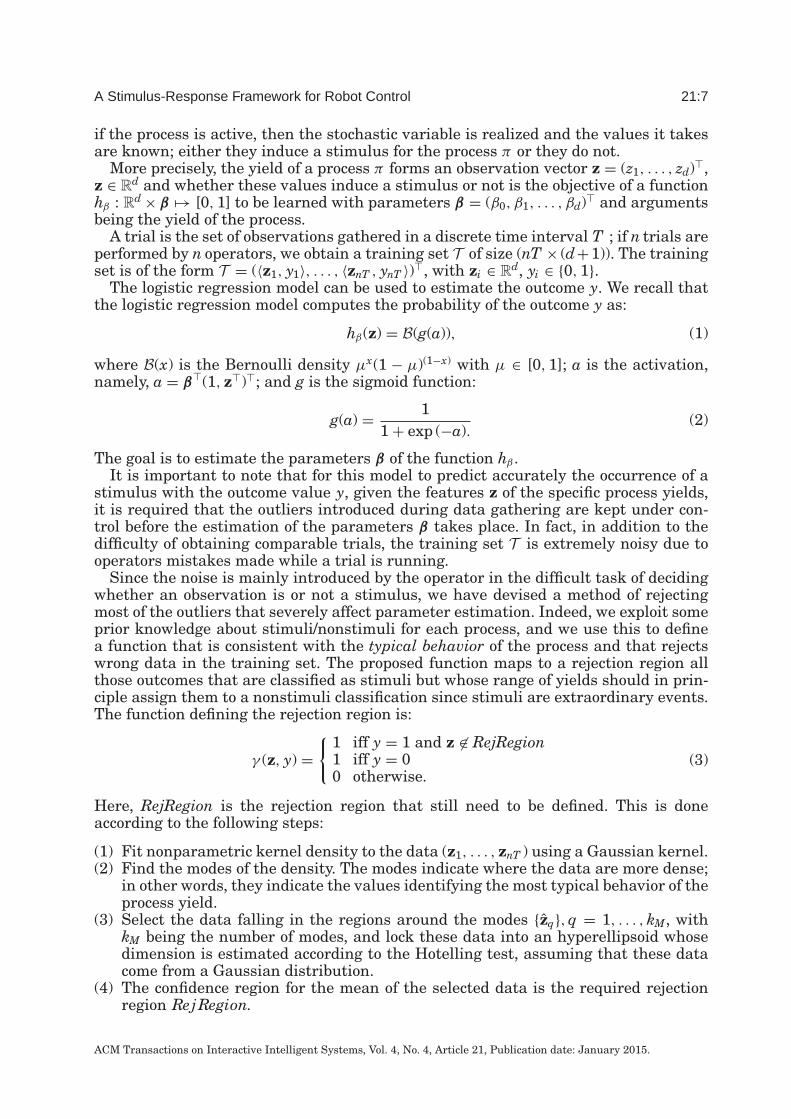
A Stimulus-Response Framework for Robot Control 21:7
if the process is active, then the stochastic variable is realized and the values it takesare known; either they induce a stimulus for the process π or they do not.
More precisely, the yield of a process π forms an observation vector z = (z1, . . . , zd)�,z ∈ Rd and whether these values induce a stimulus or not is the objective of a functionhβ : Rd × β �→ [0, 1] to be learned with parameters β = (β0, β1, . . . , βd)� and argumentsbeing the yield of the process.
A trial is the set of observations gathered in a discrete time interval T ; if n trials areperformed by n operators, we obtain a training set T of size (nT × (d+1)). The trainingset is of the form T = (〈z1, y1〉, . . . , 〈znT , ynT 〉)�, with zi ∈ Rd, yi ∈ {0, 1}.
The logistic regression model can be used to estimate the outcome y. We recall thatthe logistic regression model computes the probability of the outcome y as:
hβ(z) = B(g(a)), (1)
where B(x) is the Bernoulli density μx(1 − μ)(1−x) with μ ∈ [0, 1]; a is the activation,namely, a = β�(1, z�)�; and g is the sigmoid function:
g(a) = 11 + exp (−a).
(2)
The goal is to estimate the parameters β of the function hβ .It is important to note that for this model to predict accurately the occurrence of a
stimulus with the outcome value y, given the features z of the specific process yields,it is required that the outliers introduced during data gathering are kept under con-trol before the estimation of the parameters β takes place. In fact, in addition to thedifficulty of obtaining comparable trials, the training set T is extremely noisy due tooperators mistakes made while a trial is running.
Since the noise is mainly introduced by the operator in the difficult task of decidingwhether an observation is or not a stimulus, we have devised a method of rejectingmost of the outliers that severely affect parameter estimation. Indeed, we exploit someprior knowledge about stimuli/nonstimuli for each process, and we use this to definea function that is consistent with the typical behavior of the process and that rejectswrong data in the training set. The proposed function maps to a rejection region allthose outcomes that are classified as stimuli but whose range of yields should in prin-ciple assign them to a nonstimuli classification since stimuli are extraordinary events.The function defining the rejection region is:
γ (z, y) ={ 1 iff y = 1 and z �∈ RejRegion
1 iff y = 00 otherwise.
(3)
Here, RejRegion is the rejection region that still need to be defined. This is doneaccording to the following steps:
(1) Fit nonparametric kernel density to the data (z1, . . . , znT ) using a Gaussian kernel.(2) Find the modes of the density. The modes indicate where the data are more dense;
in other words, they indicate the values identifying the most typical behavior of theprocess yield.
(3) Select the data falling in the regions around the modes {zq}, q = 1, . . . , kM, withkM being the number of modes, and lock these data into an hyperellipsoid whosedimension is estimated according to the Hotelling test, assuming that these datacome from a Gaussian distribution.
(4) The confidence region for the mean of the selected data is the required rejectionregion Rej Region.
ACM Transactions on Interactive Intelligent Systems, Vol. 4, No. 4, Article 21, Publication date: January 2015.

21:8 M. Gianni et al.
For the first step, we consider a smoothing kernel over the process yield on a d-dimensional grid. Let x = (x1, . . . , xd) ∈ Rd be a point in the grid, and let zk ∈ Rd bean observed yield, 1 ≤ k ≤ nT = N; let υ = [( x−zk
hd )�( x−zkhd )]1/2, with h > 0 the kernel
window. We consider a radial symmetric Gaussian kernel Khd(υ) = 1√2π
exp (− 12υ2). A
nonparametric estimate for the observations that are close to point x is:
fhd(x1, . . . , xn) = 1N
N∑k=1
cKhd(υk). (4)
Here, c is the normalization term that, by the fact that∫ ∞−∞ K(υ)dυ = 1, is
(hd2(2π )(d−1)/2)−1. The gradient of the density is
∇ fhd(x1, . . . xd) ={
cN
N∑k=1
− 1h2d Khd(υk)(xj − zkj)
}j=1,...,d.
(5)
Then, by some simple algebraic transformation and hiding in c the constant term weobtain:
∇ fhd(x1, . . . , xd) ={
fhd(x1, . . . , xd)
(∑Nk=1 Khd(υk)zkj∑N
k=1 Khd(υk)− xj
)}j=1,...,d.
(6)
Local maxima of fhd are computed by gradient ascent; these are the modes z of the func-tion fhd. Let us consider these modes {zq}, q = 1, . . . , kM, with kM the number of modes.Assume these data come from a Gaussian distribution with means μq and covariances�q, and let zq and Sq be, respectively, the sample mean and sample covariance of theq-th region under the q-th mode. The confidence region at level (1 − α) for the datamean μq is:
C Rq = {μq ∈ Rd | (μq − zq)�S−1q (μq − zq) ≤ d
N − dF(1−α);d,N−d}, q = 1, . . . , kM. (7)
Here, F(1−α);d,N−d is the 1 − α quantile of the F-distribution with d and N − d degreesof freedom. That is, we are confident at a level (1 − α) that C Rq contains μq; namely,p(μq ∈ C Rq) = (1 − α). Now, (μq − zq)�S−1
q (μq − zq), q = 1, . . . , kM are hyperellipsoids
with center μq and semi-axes of length√
D2qλsq, where λsq is the s-th eigenvalue of
S−1q . Since D2
q = dN−d F(1−α);d,N−d is the maximal ellipsoid surface, enclosing the q-th
confidence region, it follows that these regions correspond to the most typical behaviorof the yield of the process π under consideration. Hence, these are rejection regions forstimuli—regions where it is most unlikely that a stimulus can occur. Therefore, we arefinally arrived at the definition of rejection region RejRegion:
RejRegion = {z ∈ Rd |(zq − z)�S−1q (zq − z) ≤ D2
q, q = 1, . . . kM}. (8)
As noted earlier, kM is the number of modes of the nonparametric density. Therefore,according to Equation (3), the set of samples for which γ (zk, yk) > 0, k = 1, . . . , N (recallthat N = nT ) is the optimal one for classification.
Now, given a complete set of good samples T � = (〈z1, y1〉, . . . , 〈zN, yN〉), the model forstimulus prediction is provided by logistic regression. Namely, the logistic regressioncoefficients β are obtained from the good trial set T � for the yield of process π by
ACM Transactions on Interactive Intelligent Systems, Vol. 4, No. 4, Article 21, Publication date: January 2015.

A Stimulus-Response Framework for Robot Control 21:9
Table II. Components, Processes, and Stimuli
Component Description Process Description Stimulus Description
Battery Power Level Monitoring Battery ExhaustionWiFi Connection Management WiFi DisconnectionRobot Engine Temperature Monitoring Temperature LevelVisual Perception Detecting Object/Person Detected Object/PersonMemory Data Writing Write Access to Memory FullDialogue Human to Robot Exchanging msg Human to Robot Message
minimizing the following cost function:
L(β) = −1n
(N∑
i=1
yi log hβ(zi) + (1 − yi) log(1 − hβ(zi))
)+ ξ
2n
d∑j=1
β2j . (9)
Here, ξ is the regularization parameter and∑d
j=1 β2j the regularization term; these
are used just in case the features induce a high-dimensional space, which in generalis kept ≤ 5 to manage the nonparametric density. The Newton-Raphson algorithmused to minimize Equation (9) requires an update step expressed as a least squarestep, namely, as an iteratively reweighted least square. Then, given a new observationz�, hβ(z�) is the hypothesis returning the binary response within the variable y. Moreprecisely:
y ={
1 if hβ(z�) ≥ 0.50 if hβ(z�) < 0.5.
(10)
We have thus provided a model to represent the stimuli and for learning when suchstimuli occur. We have also introduced the principle that a large region of nonstimulifor each process yield can be identified around the most typical values of the yield tosimplify noisy data collection. Note that this concept of typical values for the processyield grants the possibility of estimating hβ with quite few trials.
4. THE STIMULUS-RESPONSE MATRIX
Given a process π, we have introduced the function hβ that takes as input the yield ofa process and determines whether a stimulus is triggered or not, returning a value 1if this is the case and a value 0 otherwise. If a stimulus occurs, it is necessary to scoreall possible response tasks before any decision can be taken.
In this section, we show how to score the relation stimulus response, which amountsto scoring the task that would eventually be chosen to respond to the triggered stimulus.Here, a task is a set of processes; see Table II for an excerpt of the structures linkingrobot components, processes, and stimuli, and the more detailed Tables VI, VII, andVIII in Appendix A. Therefore, while a task is being executed, a stimulus can betriggered from any of the active processes of the task. To address each case, given alimited number of tasks for a robot, we introduce a stimulus-responses matrix A thatscores each pair: The score matrix A is formed by two classes of entities, which we referto as Tasks (rows) and Stimuli (columns), respectively (see Table VII and Table VIII inAppendix A). Note that a task is built out of many processes, yet each process can yielda single stimulus; namely, there is a bijection between each process and the stimulusit yields.
Matrix A is initially built using a number of experiments and further completed byestimating the unknown values for the stimulus-response pairs with the regularizedlow-rank matrix factorization method [Zhang et al. 2012; Chen 2008; Buchanan andFitzgibbon 2005; Canny 2002].
ACM Transactions on Interactive Intelligent Systems, Vol. 4, No. 4, Article 21, Publication date: January 2015.

21:10 M. Gianni et al.
The experiments for filling A are short-term missions performed by operators whoare well informed about the task library, the processes, and the stimuli that the robotcan handle. Each operator is assigned a task from the task library (see Table VII inAppendix A, as described in Section 7). During the trial, a stimulus is triggered for anactive process π j . Upon the occurrence of the stimulus, the operator selects the task τithat he or she considers the most appropriate to respond to the presented stimulus fromamong those reported in Table VII (Appendix A) using a graphical user interface (seeFigure 11 in Appendix A). Note that, during the experiment, the operator teleoperatesthe robot. The experiment terminates when the operator signifies his or her task choice.Data from each trial, reporting the occurrence of the pairs 〈τi, yπ j 〉, are collected, andthe corresponding entries aij of matrix A (see Table IX and Table X ) are filled. Whenoperators did not select the corresponding stimulus-task pair, a dash sign is added.
The problem now is to complete the matrix by finding the missed values. These arerecovered by factorizing matrix A into the product of two smaller matrices, P ∈ Rm×d
and Q ∈ Rn×d, of rank d1. Given that A has dimension (n × m)—namely, n tasks andm process yields (here, n = 13 and m = 42)—and rank d, in order to complete A, it isnecessary to find two factors explaining A: an (n × d) matrix Q and an (m× d) matrixP, such that A = QP� . Thus, it is possible to minimize the error norm on the knownvalues.
Let W be an indicator matrix of the same size as A in which 0’s correspond tomissing elements of A and 1’s correspond to observed data; then, the problem can bereformulated as:
ε(Q, P) = ‖W � (A − QP�)‖2F + λ1‖Q‖2
F + λ2‖P‖2F . (11)
Here, � is the Hadamard component-wise matrix product, ‖ · ‖ is the Frobenius norm,and λ1 and λ2 are regularizing constants. Several approaches have been proposed tominimize this error, considering that if one of Q or P are known, there is a closed-formsolution for the other that minimizes Equation (11) (see, e.g., the dumped Newtonalgorithm introduced by Buchanan and Fitzgibbon [2005] and the Wieberg algorithmof Takayuki Okatani and Deguchi [2006]). Here, we have chosen a version of thealternating-least-squares with weighted-λ-regularization [Zhou et al. 2008], in whichthe steps to obtain Q and P are summarized as follows. Initialize Q and P to smallrandom values and let wi j be the (i, j) element of the indicator matrix W; then, theschema (11) can be rewritten as follows:
ε(q1, . . . , qn, ρ1, . . . , ρm)) = 12
∑(i, j)
wi j(ρT
j qi − aij)2 + b1
2
n∑i=1
d∑k=1
q2ik + b2
2
m∑j=1
d∑k=1
ρ2jk. (12)
Here, the first term of Equation (12) corresponds to the square error term, and the lastterms are the regularization terms of qi and ρ j , respectively. The terms b1 and b2 are theregularization parameters. Local optima of the objective function in Equation (12) arefound via Newton-Raphson gradient descent. The update rules, for every i = 1, . . . , nand for every j = 1, . . . , m are given by the following equations:
qik := qik − ζ1
⎛⎝∑j
wi j(ρT
j qi − aij)ρ jk + b1qik
⎞⎠ρ jk := ρ jk − ζ2
(∑i
wi j(ρT
j qi − aij)qik + b2ρ jk
) . (13)
1Here, the letter d is used for the matrix rank, while in the previous section it was used to define the size ofobservations.
ACM Transactions on Interactive Intelligent Systems, Vol. 4, No. 4, Article 21, Publication date: January 2015.
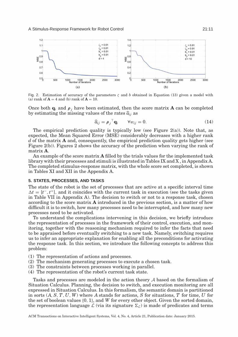
A Stimulus-Response Framework for Robot Control 21:11
Fig. 2. Estimation of accuracy of the parameters ζ and b obtained in Equation (13) given a model with(a) rank of A = 4 and (b) rank of A = 10.
Once both qi and ρ j have been estimated, then the score matrix A can be completedby estimating the missing values of the rates ai j as
ai j = ρ j�qi ∀wi j = 0. (14)
The empirical prediction quality is typically low (see Figure 2(a)). Note that, asexpected, the Mean Squared Error (MSE) considerably decreases with a higher rankd of the matrix A and, consequently, the empirical prediction quality gets higher (seeFigure 2(b)). Figures 2 shows the accuracy of the prediction when varying the rank ofmatrix A.
An example of the score matrix A filled by the trials values for the implemented tasklibrary with their processes and stimuli is illustrated in Tables IX and X , in Appendix A.The completed stimulus-response matrix, with the whole score set completed, is shownin Tables XI and XII in the Appendix A.
5. STATES, PROCESSES, AND TASKS
The state of the robot is the set of processes that are active at a specific interval time�t = [t−, t+], and it coincides with the current task in execution (see the tasks givenin Table VII in Appendix A). The decision to switch or not to a response task, chosenaccording to the score matrix A introduced in the previous section, is a matter of howdifficult it is to switch, how many processes need to be interrupted, and how many newprocesses need to be activated.
To understand the complications intervening in this decision, we briefly introducethe representation of processes in the framework of their control, execution, and mon-itoring, together with the reasoning mechanism required to infer the facts that needto be appraised before eventually switching to a new task. Namely, switching requiresus to infer an appropriate explanation for enabling all the preconditions for activatingthe response task. In this section, we introduce the following concepts to address thisproblem:
(1) The representation of actions and processes.(2) The mechanism generating processes to execute a chosen task.(3) The constraints between processes working in parallel.(4) The representation of the robot’s current task state.
Tasks and processes are modeled in the action theory A based on the formalism ofSituation Calculus. Planning, the decision to switch, and execution monitoring are allexpressed in Situation Calculus. In this formalism, the semantic domain is partitionedin sorts (A, S, T ,U, W) where A stands for actions, S for situations, T for time, U forthe set of boolean values {0, 1}, and W for every other object. Given the sorted domain,the representation language L (via its signature �L) is made of predicates and terms
ACM Transactions on Interactive Intelligent Systems, Vol. 4, No. 4, Article 21, Publication date: January 2015.

21:12 M. Gianni et al.
(variables and functions of arity n ≥ 0) and ruled by the first-order predicate calculus,with the exception of an inductive axiom. We refer the reader to Pirri and Reiter [1999]for a full description of the formalism. The representation language is used to providethe robot with a reasoning and knowledge structure about actions by specifying theirpreconditions and effects, and about both the processes and the constraints linkingtheir parallel execution.
A process is a predicate π (x, u, t, do(a, s)) taking as arguments a single term u of sortboolean for the stimulus, a term t of sort time, a single term do(a, s) of sort situation,and terms x = (x1, . . . , xn), n ≥ 0 of any other sort. The special function do of sortsituation is an action sequence builder that defines a situation as a list of actions. Moreprecisely, do is a function taking as arguments a term of sort action and a term of sortsituation and returning a term of sort situation do : A × S �→ S, which is a list ofactions. Actions are functions, and when the term of sort situation explicitly mentionsthe sequence of actions it builds, we denote the term with σ . Through its arguments,a process carries the information about the history of all processes of a component viaall its start and end actions, activated up to the time t. For example, consider one ofthe processes given in Table VI, Appendix A: The connection management of the WiFicomponent is represented in language L by the following transition statement:
πWiFi(x, u, t, do(a, s)) ≡ [a = startWiFi(x, t) ∧ u = 0] ∨ (∃t′.t′ ≤ t ∧ πWiFi(x, u, t′, s)∧(∀t′′∀u.(t′′ > t′ ∧ t′′ ≤ t)→E(x, t′′) = u→a �= endWiFi(x, t′′))).
(15)Here, startWiFi and endWiFi are actions, and t, t′, t′′ are variables of sort time. Thefunction E maps terms of the representation language L to the values identified by thestimulus model (Section 3). This function takes as input the realization of the yieldsof the process when the process is active, and it returns the value u = 1 if the signalelicits a stimulus and u = 0 otherwise. This is called a transition axiom, and it specifiesthat the robot process managing WiFi connection is active if either the action startWiFiis executed at time t, or the process was already active at some previous time t′, and,at any time between t′ and t (the current time), it was not ended by a disconnectionnotified by a stimulus nor it was ended by the action endWiFi independently of thestimulus value. The transduction of a stimulus realization to a term of the languageL requires the existence of a set of transformations binding terms and domains atexecution time. This is better detailed by the following remark.
Remark 5.1 (Transduction between stimuli and processes). A process yield and itsstimulus value are both linked to the signature �L of the action language L by themapping E . The domain of L and of the processes’ yields are linked by the interpretationI of L.
To prove this, we first introduce some auxiliary mappings. Let L be a set of labels,and let T be time. We introduce the function E+ : Rn × L → �L, the function E� :[0, 1] × T → �L, and finally the mapping re : Rn × T �→ Rn and the mapping E :�L × T �→ �L. To these functions, we add the interpretation function I mappingterms of the language into the interpretation domain, and we assume that equalityis interpreted by itself. We have to show that, via E�, re, and E+, E links the featureterms with terms of L and that the interpretation links, via the mappings, the sampledomain where the yields take values with the domain of interpretation for L. Let usassign to each defined process π ∈ L a label, and let X : �n �→ Rn be a multivariaterandom variable whose realizations are the observed values z of the yield of π attime t. The function re serves to specify the realization with respect to the processyields and time, namely, re(X, t) = z ∈ Rn. Now E+ maps real numbers, labeled bythe specific process of which they are the yield, into terms of the language such as
ACM Transactions on Interactive Intelligent Systems, Vol. 4, No. 4, Article 21, Publication date: January 2015.

A Stimulus-Response Framework for Robot Control 21:13
E+([z3, z4], LWiFi) = (signal strength, distance f rom source) and so on. Similarly, E�
takes the outcome of the learning function hβ(z) (see Section 3) and maps it to a term ofthe language. These terms have a semantics in the domain Dn of L, so that real valueslabeled by a process name need to be paired with the interpretation of the terms of thespecific process. So, for example, the interpretation of the term signal strength ∈ �L,taken as argument by the process π , has to be linked to the corresponding element ofthe sample domain �n. Therefore, when the process is active, then t is instantiated,the transduction closes the loop between the different terms, and binding occurs on theappropriate instances in the respective domains according to the sorts requirements:
re(X, t) = z ∈ Rn
E+(z, L) = x ∈ �LE�(hβ(z), t) = u ∈ �LuI ∈ {0, 1} ⊂ DE(E+(re(X, t), L), t) = E(x, t) = E�(hβ(z), t) = u ∈ �LE I(E+(re(X, t), L), t)I = E�,I(hβ(z), t)I = uI ∈ {0, 1} ⊂ D.
(16)
This shows that the mappings E�, E+, re, and E , together with the interpretation I ofthe language, are sufficient to define the transduction between stimuli and processes,both linking the terms of the language and mapping the outcome into {0, 1} ⊂ D.
A process π is active between a startπ and an endπ action. To activate a start or endaction, a special predicate Poss tells the robot whether the action can be done giventhe current situation s and time t, for example:
Poss(endWiFi(x, t), u, s) ≡(at(home, t, s) ∧ ¬ask(operator, t, s) ∨ u = 1) ∧ πWiFi(x, u, t, s) (17)
tells the robot that the WiFi process can be ended if it is at home and if, for exam-ple, there are no operator requests running or a disconnection signal is detected. Thisstatement is called a precondition axiom. Note that a state is defined by all the pred-icates (processes and facts) that are verified at the specific situation and time in theintended model. Thus, if M is the model of the language satisfying the whole theory,we might say that M |= ∧
ϕ(t, σ ) to indicate that the finite set of sentences∧
ϕ holdsat time t in situation σ in the model, and so specify a finite state of the system. Onthe other hand, we can also write A |= ∃x, u, t.πC(x, u, t, σ ) to indicate that all themodels (actually the intended model of the axiomatization) of the action theory A arealso models of the process πC at some time t and situation σ , thus indicating that thesituation σ = do(An(x), do(An−1(x), . . . , do(A1(x), S0)) . . .) returns a sequence of actionsthat governs the processes that can be activated in S0 to perform some task involvingthe component C.
Robot components are both hardware devices and software modules such as engines,dialog, vision, mapping, planning, path planning, and so on, all handling several pro-cesses and needing to be regulated not only by transition and precondition axioms, butalso by both temporal and spatial relations. To handle relations between processes, aparallelization of situations into several timelines has been introduced [Finzi and Pirri2010], and each timeline assesses the evolution of all the processes of a component. Atimeline is a special situation taking into account only the start and end actions of theprocesses of a component. Parallel situations are handled by a set of situations calledbags of timelines. Time constraints are based on the definition of the greatest starttime and least end time, thus bounding a process activity within a start and end time,up to a fixed time t. The greatest start time is defined as:
greatestStartπ (x, a, t)def≡ ∃t′.a = startπ (x, t′)∧¬∃t′′, a′′.t′ ≤ t′′ ≤ t∧a′′ = endπ (x, t′′). (18)
ACM Transactions on Interactive Intelligent Systems, Vol. 4, No. 4, Article 21, Publication date: January 2015.

21:14 M. Gianni et al.
An analogous definition is given for leastEnd, the least end time for an action, thuscharacterizing the �t inside which a process is certainly active or certainly not active.Given this definition, a time relation such as during is defined as follows:
{πi(x, u, t, do(a, σ )) during π j(x′, u′, t′, do(a′, σ ′))}[ , ′]
def≡σ ∈ ∧ σ ′ ∈ ′ ∧ πi(x, u, t, do(a, σ )) ∧ π j(x′, u′, t′, do(a′, σ ′))∧[greatestStartπi (x, a, t) ≥ greatestStartπ j (x′, a′, t′)]∧[leastEndπi (x, a, t) ≤ leastEndπ j (x′, a′, t′)].
(19)Here, and ′ are bags of timelines; specifically, timelines of different robot com-ponents. Note that in the formulas specifying constraints (as in Equation (19)),the variables have a lambda binding, which means that the variables are bound bythe quantifiers inside the sentence in which they are embedded because the timeconstraints are macro sentences of the language. Temporal constraints are typicallythose defined in Allen [1983], among which we consider the set {during, bef ore,meet, start, f inishes, overlaps, equal}.
For example, the Equation (20) says that to start the process of approaching a certainlocation, the path planner process needs to be active, which in turns requires themapping to be active:
[πpath−planning(x, u, t, σ ) during πmapping(x′, u′, t′, σ ′)]before πapproach(x′′, u′′, t′′, σ ′′)[ , ′, ′′] (20)
A constraint formula is indicated by πiopπ j[ i, j], and a set of constraint formulas isindicated by C. Note that constraints are special formulas because only the definiens(namely, the left hand side of the definitions) are expressed in the language L.
Different approaches for defining constraints in a first-order language have beenproposed [Baar et al. 2001; Block et al. 2006; Morris et al. 2001; McDermott 2003; Foxand Long 2003; Carbone et al. 2008; Wittocx et al. 2010]. A definition for each timeconstraint between processes, according to linear interval-based time [Allen 1983], isprovided in Finzi and Pirri [2010].
Similar to temporal constraints, spatial constraints are defined following the topo-logical relations introduced in Randell et al. [1992]. Spatial and time constraints (seeWolter and Zakharyaschev [2000] and Finger and Gabbay [1996]) are integrated in theframework.
Now we must specify what happens if the robot needs to switch to a different taskand stop the current one. If at time t, the robot has to infer the processes needed toexecute a task , it may be that for some process the starting action startπ or the endingaction endπ are not derivable; namely, A ∪ C �|= ∃x, t Poss(startπ (x, t), σ ). To modify thecurrent execution and make the activation of a process possible, it is desirable to obtainan explanation for enabling a specific action a. This is the formula ψ ∈ L, such that:
A ∪ C ∪ {ψ} �|=, and A ∪ C ∪ {ψ} |= ∃x, t Poss(startπ (x, t), σ ), (21)
where the proviso A ∪ C ∪ {ψ} �|= means that the explanation added to the theory doesnot imply the contradiction. Explanations can be computed using first-order abduction(see, e.g., Marquis [1991] and Cialdea and Pirri [1993]). Here, A is the action theory, C isthe set of temporal-spatial constraints, and ψ is the formula explaining the observation∃x, t Poss(startπ (x, t), σ ); that is, ψ is the formula to be added to ensure the inference.
Examples of such processes are reported by Finzi and Pirri [2005, 2010], Carboneet al. [2008], Pirri and Reiter [2000], and Pirri [2011] in the framework of Situa-tion Calculus [Pirri and Reiter 1999]. However, processes are defined in several otherframeworks, as, for example, in STRIPS, Graphplan, and PDDL [Blum and Langford
ACM Transactions on Interactive Intelligent Systems, Vol. 4, No. 4, Article 21, Publication date: January 2015.

A Stimulus-Response Framework for Robot Control 21:15
1999; McDermott 2003; Fox and Long 2003; Fikes and Nilsson 1971]. Each of thesehas its own advantages in terms of expressive power, computational feasibility, andconstraints expressible in the language. When robot planning requires the orchestra-tion of all components according to temporal constraints, the planning system usuallytakes advantage of temporal networks to manage temporal constraints [Allen 1983;Dechter et al. 1991; Vilain et al. 1986; Block et al. 2006; Morris et al. 2001]. Here,we use Situation Calculus to model high-level control of robot processes because of itsexpressive power both for managing parallel processes and time-space constraints andfor defining interference and reconfiguration cost. The stimuli and stimulus-responsemodel proposed in this work could be built on any action theory that handles robotcomponents, processes, and constraints and is able to express robot mental state ata precise time, together with all cause-effect relations affected by the response. Thisneed is clarified in the next section, where we compute the cost of an explanation.
6. TO SWITCH OR NOT TO SWITCH
We are now at a point in the formalization of the stimulus-response where we canillustrate how a decision can be taken about whether to respond to a stimulus. Toillustrate the decision problem, we continue with the WiFi disconnection example.
Example 6.1. The robot is executing task τ10, expecting to approach victims ina rescue area. At time t, the process πWiFi get disconnected, hβ(zWiFi) = 1; henceE(xWiFi, t) = 1. Therefore, the action endWiFi becomes possible, and process πWiFi isinterrupted. From table A, the robot is advised to switch to task τ4, which correspondsto recovery WiFi signal, so it can choose between continuing the current task withoutthe WiFi signal or switching to task τ4. To make the switch, it has to discontinueseveral active processes in τ10 (see the Table VII in Appendix A), and it has to activateonly process π1,C11 , which is read access to missing data, because all others requiredprocesses are already active in τ10. However, the constraints of the kind πiopkπ j in theprocesses have changed, and they need to be recomputed in the new task τ4. Therefore,the system has to rate the effort and risks that its choice implies.
Here, we assume that before any decision to switch is taken, the response tasks toswitch to has been selected according to the scores given by matrix A (see Section 4).We first consider the switching cost, given the best scored task to switch to. The costto switch from the current to a new task breaks down into a reconfiguration and aninterference cost with respect to a specific task. To these costs we may add a secondreconfiguration cost if we need to return to the current task.
Reconfiguration cost: This is the cost to reconfigure the current robot state, whichamounts to activating new processes πR1 , . . . , πRm. More precisely, the reconfigurationcost calculates the effort the system has to invest to infer all the transition and precon-dition axioms that are required to make processes πR1 , . . . , πRm executable by the robotat the current state.
Interference cost: This is the cost needed to terminate active processes πS1 , . . . , πSk
specifying the current task, which are either not needed or would hinder the newlychosen task.
Let τi be the current task under execution, and let τ j be a chosen task. Let �R ={πR1 , . . . , πRm} be all the processes that need to be activated to operate task τ j and whichare not yet active, and let �S = {πS1 , . . . , πSk} be all the active processes that need tobe turned off. Then, according to Equation (21), there is a set of formulas � and a setof formula � that must be inferred to explain, respectively, how processes �R can be
ACM Transactions on Interactive Intelligent Systems, Vol. 4, No. 4, Article 21, Publication date: January 2015.

21:16 M. Gianni et al.
activated and how processes �S can be turned off:
A ∪ C ∪ � |= ∃x, t∧m
i=1 Poss(startπRi(x, t), σ ) ∧ ∧
i �= j πRi opπRj [ i, j], ∀πRi ∈ �R
A ∪ C ∪ � |= ∃x, t∧k
i=1 Poss(endπSi(x, t), σ ) ∧ ∧
i �= j πSi opπSj [ i, j], ∀πSi ∈ �S.
(22)Note that � and � are not necessarily minimal explanations (see Marquis [1991] andCialdea and Pirri [1993] for the minimality problem in computing first-order explana-tions), but we might assume here that these explanations nevertheless minimize theaction sequences.
The cost of reconfiguration and interference amounts to computing the cost of thesestatements. We define the cost considering first the terms of the language; namely,variables and functions of any arity. We exclude from the cost evaluation the termsmentioning variables of sort situation and variables of sort action: For example do(a, s)is excluded, but not do(A(x), S0) since S0 is a constant of sort situation and the actionterm A is not a variable. Let η be a term of the language; the cost of η is inductivelygiven by the function ν, defined as follows:
ν (η) =⎧⎨⎩
0 if η does not mention terms of sort action1 if η = startπ (x, t) or η = endπ (x, t)∑k
i=1 ν (Ai) if η mentions A1, . . . , Ak terms of sort action(23)
Here, t is a term of sort time and x is a list of terms (i.e., variables, constants,functions of any arity) of any sort. Now, to extend the cost computation to formulas,we consider the following restrictions. Let ϕ ∈ L; we assume that ϕ either does notmention terms of sort action and situation or, if it does mention them, these are inthe form do([A1, . . . , Am]), with none of the action terms Ai as variables. Then, letDNF(ϕ) = Qx[C1(x1) ∨ · · · ∨ Cm(xm)] ≡ ϕ be the equivalent transformation of ϕ intoDNF; namely, into disjunctive normal form in which each clause Ci(xi), 1 ≤ i ≤ m,is a conjunction of literals, with xi terms varying on all sorts. Variables mentioned inxi are included in x and bound by the quantifiers matrix Qx. Clearly, any variable xappearing in xi can neither be of sort action nor situation. Then the cost of the formulaϕ is inductively defined as follows:
cost (ϕ) =⎧⎨⎩
ν (x) if ϕ = L (x) is a literal∑i cost (Li (xi)) if ϕ ≡ Qx
(L1(x1) ∧ · · · ∧ Lk(xk)
)min{cost(Ci(xi))} if ϕ ≡ Qx
(C1(x1) ∨ · · · ∨ Cm(xm)
) (24)
Note that if ϕ is a tautology, then ϕ can be reduced to a tautology—namely ϕ ≡B∨ ¬B∨ C, for any clause C. Hence, min{cost(ϕ)} = 0, since B does not mention termsof sort action. On the other hand, if ϕ is a contradiction, then ϕ ≡ B∧¬B∧∧
i ψi for anyconjunction
∧i ψi of literals of L. Hence, cost(ϕ) = min{∑i cost(Li)}, with
∑i cost(Li)
tending to infinity since we may take any literal from the language and with anysequence of actions as argument. Finally, given a set of formulas �, the cost of � is thesum of the costs of each ψ ∈ �.
We are now ready to determine the cost for inferring the explanations needed toactivate a preferred task τ j in terms of the cost of the preconditions and constraintsfor τ j , at time t, according to Equation (22) and in terms of discontinuing a number ofprocesses occurring in the current task τi. Given Equation (22), the cost of inferencefor switching is:
switchCost(〈τ j, τi〉, t) = cost(�, t) + cost(�, t) + J cost(� ′, t′), t′ > t, q ∈ {0, 1}. (25)
ACM Transactions on Interactive Intelligent Systems, Vol. 4, No. 4, Article 21, Publication date: January 2015.

A Stimulus-Response Framework for Robot Control 21:17
Fig. 3. The switching costs for the task τ12, data retrieval (see Table VII ). The up-rows indicate the processesthe task is assembled from and their yields. In the left column are the tasks that obtained the maximumswitching score in score matrix A. The gray cells indicate the average normalized switching cost to thepreferred task, indicated in the left column.
Here, � ′ is like �, but it is the cost of returning to the current task after the task therobot has switched to is completed. If J = 0, there is no need to return to the currenttask τi.
Having obtained the switching cost and knowing the response task for the triggeredstimulus, we can compute the payoff. Here, the payoff is simply the culmination ofthe stimulus-response problem and it is, indeed, the payoff for switching. Let RS be afunction specifying the choice of switching and RI the analogous function for inhibition.Then the payoff for switching is simply RS − RI .
Obviously, we expect to attribute the switching cost to RS. However, if the switchingcost is computed before any decision is taken, then this is like attributing the cost toboth RS and RI . In fact, by its definition, computing the switching cost is the same asabducing the set of explanations needed to activate the new task and deactivating thecurrent state; thus, it follows that this inference process ends up weighting the decisionwell before the decision is taken.2
Therefore, to both correctly define the two functions and to avoid burdening thedecision, the switching cost can be replaced by a prediction of it. To predict the switchingcost, as defined in Equation (25), two steps are needed:
(1) Define a trend of the switching cost according to time, in terms of the sequence ofactions entering the σs of the two logical implications in Equation (22).
(2) Produce an estimate of the switching cost for different time durations of the currenttask.
To this end, we generate a number of action sequences for as many time lapses withina time range bounded by 120 minutes. For each of these samples, the cost given inEquation (25) is computed. An example of the averages of the normalized switchingcost for task τ12—namely, data retrieval—is given in Figure 3 with respect to each of theresponse tasks to the stimuli that can be triggered by each of the processes composingthe execution of task τ12.
The trends of the switching cost for a task are established with respect to each ofits processes and for each of the response tasks to the stimuli of its process yields;therefore, it is defined for each pair 〈τi, τ j〉. Once the trends are obtained, the switchingcost is approximated by its frequencies with respect to time.
To estimate the cost distribution, we define a bivariate random variable X takingvalues in the domain T imes × SwitchingCost for each pair 〈τi, τ j〉. The realization ofthe bivariate variable X is computed by a nonparametric density fX measuring theswitching cost frequencies to discontinue the current task τi and activate task τ j . Here,we use a Gaussian kernel to estimate kernal density, as we did in Section 3; here,however, we have a bivariate estimator (time and cost), so we define the kernel density
2Computing the explanations for switching can be viewed as the intellectual work that the system performs,as opposed to the practical and physical work of executing tasks.
ACM Transactions on Interactive Intelligent Systems, Vol. 4, No. 4, Article 21, Publication date: January 2015.

21:18 M. Gianni et al.
Fig. 4. Kernel density fX for switching cost from the task τ12 to task τ4, showing frequencies of switchingcost in a time lapse of 120 minutes, taken with respect to 10 cost trends.
for a generic task as follows:
fX(x) = 1n
n∑i=1
1det(H)
K(diag(H−1)�(x − Xi)). (26)
Here, K(υ) = 1√2π
exp (− 12υ2) and H = n−1/6�1/2, where � is the diagonal covariance
matrix of the samples; namely, H follows the Scott’s rule of thumb, and diag(·) indicatesthe diagonal. The grid has resolution H, and the bivariate Xi is built using samplesfrom the switch cost trend taken at time t for different action sequences. The switchingcost density for tasks (τ12, τ4) is illustrated in Figure 4, where time is presented inminutes. To compute the modes of kernel density, we proceed as in Section 3. Letυi = diag(H−1)�(x − Xi) and diag(H) = (h1, h2)�; then the gradient of fX is:
∇ fX(x1, x2) ={
1n
n∑i=1
− 1hjdet(H)
K(υi)υi
}j=1,2
={
− fX(x1, x2)
(x1
h2j
+ x2
det(H)
)
+1n
n∑i=1
1det(H)
K(ui)
(Xi1
h2j
+ Xi2
det(H)
)}j=1,2
(27)
As in Section 3, the modes x are collected by gradient ascent. The modes return thebest prediction of the bivariate x. Where the probability of x is below a threshold ε orwhere the probability is high but the estimated switching cost (given time t) is beyondthe effort the robot system can afford, then we introduce a time failure. These failures,that can be collected for each pair 〈τi, τ j〉, are best explained with an example.
Example 6.2. Continuing Example 6.1, consider the pair (τ10, τ4) at time t = 72.According to the cost trends, the nonparametric function fX(x) is drawn, and it hasmodes at T = (35, 71, 110, 119). At these times, the cost rates are (0.3, 0.5, 0.7, 0.9).Let ε = 0.6 be the maximum cost the robot can afford to switch. Since t = 72, it follows
ACM Transactions on Interactive Intelligent Systems, Vol. 4, No. 4, Article 21, Publication date: January 2015.
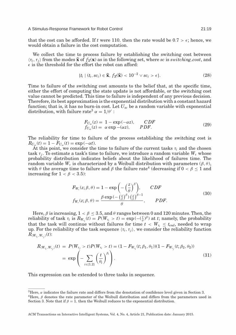
A Stimulus-Response Framework for Robot Control 21:19
that the cost can be afforded. If t were 110, then the rate would be 0.7 > ε; hence, wewould obtain a failure in the cost computation.
We collect the time to process failure by establishing the switching cost between〈τi, τ j〉 from the modes x of fX(x) as in the following set, where sc is switching cost, andε is the threshold for the effort the robot can afford:
{ti | (ti, sci) ∈ x, fX(x) < 10−2 ∨ sci > ε}. (28)
Time to failure of the switching cost amounts to the belief that, at the specific time,either the effort of computing the state update is not affordable, or the switching costvalue cannot be predicted. This time to failure is independent of any previous decision.Therefore, its best approximation is the exponential distribution with a constant hazardfunction; that is, it has no burn-in cost. Let Usc be a random variable with exponentialdistribution, with failure rate3 α = 1/θ ′ :
FUsc (z) = 1 − exp (−αz), CDFfUsc (z) = α exp −(αz), PDF.
(29)
The reliability for time to failure of the process establishing the switching cost isRUsc (t) = 1 − FUsc (t) = exp (−αt).
At this point, we consider the time to failure of the current tasks τi and the chosentask τ j . To estimate a task’s time to failure, we introduce a random variable Wτ whoseprobability distribution indicates beliefs about the likelihood of failures time. Therandom variable Wτ is characterized by a Weibull distribution with parameters (β, θ ),with θ the average time to failure and β the failure rate4 (decreasing if 0 < β ≤ 1 andincreasing for 1 < β < 3.5):
FWτ(z; β, θ ) = 1 − exp
(−
( zθ
)β)
, CDF
fWτ(z; β, θ ) = β exp (− ( z
θ
)β)( z
θ
)β−1
θ, PDF.
(30)
Here, β is increasing, 1 < β ≤ 3.5, and θ ranges between 0 and 120 minutes. Then, thereliability of task τi is RWτi
(t) = P(Wτi > t) = exp (−( tθ)β) at t; namely, the probability
that the task will continue without failures for time t < Wτi ≤ tend, needed to wrapup. For the reliability of the task sequence 〈τi, τ j〉, we consider the reliability functionR〈Wτi ,Wτ j 〉(t):
R〈Wτi ,Wτ j 〉(t) = P(Wτ j > t)P(Wτi > t) = (1 − FWτi(t; β1, θ1))(1 − FWτ j
(t; β2, θ2))
= exp
⎛⎝−∑
i∈{1,2}
(tθi
)βi
⎞⎠ .(31)
This expression can be extended to three tasks in sequence.
3Here, α indicates the failure rate and differs from the denotation of confidence level given in Section 3.4Here, β denotes the rate parameter of the Weibull distribution and differs from the parameters used inSection 3. Note that if β = 1, then the Weibull reduces to the exponential distribution.
ACM Transactions on Interactive Intelligent Systems, Vol. 4, No. 4, Article 21, Publication date: January 2015.

21:20 M. Gianni et al.
Fig. 5. Examples of reliability of the current task (the dashed black line) against the reliability of theparallel composition of the switching cost reliability with the sequence formed by the current task τi and thechosen task τ j .
Finally, the reliability of the combination of the two tasks, taken in sequence, and theswitching cost estimation, taken in parallel with the two tasks, is defined as follows:
R(〈Wτi ,Wτ j 〉||Usc)(t) = P(Wτ j >t)P(Wτi >t) + P(Usc > t) − P(Wτ j >t)P(Wτi >t)P(Usc>t)
= exp (−tα) + exp
⎛⎝−∑
i∈{1,2}
(tθi
)βi
⎞⎠ − exp
⎛⎝−tα −∑
i∈{1,2}
(tθi
)βi
⎞⎠.
(32)At this point, we can see that R(〈Wτi ,Wτ j 〉||Usc)(t) and RWτi
(t) are the two sought for functionsRS and RI introduced earlier, and, therefore, the payoff for switching is:
payoff = R(〈Wτi ,Wτ j 〉||Usc)(t) − RWτi(t). (33)
Clearly, if at the given time t, RWτi(t) < R(〈Wτi ,Wτ j 〉||Usc)(t), then the payoff is positive
and switching is convenient; otherwise it is negative or null. Some examples showingreliability are illustrated in Figure 5. The simulation-based computation for task timeto failures is reported in the Appendix A.7, and experiments computing the payoff forswitching are reported in Section 7.3.
7. EXPERIMENTS
In this section, we present the results of experiments undertaken to evaluate the pro-posed framework’s performance. In Section 7.1 , the performance of the stimulus modelis tested. In Section 7.2, we evaluate the generalizability of the score matrix A, de-scribed in Section 4. In Section 7.3, we test the switching decision described in Section 6.The whole framework is tested in Section 7.4. Finally, in Section 7.5, we comparethe performance of the stimulus-response framework with two different approaches torobot replanning [Beetz et al. 2010; Talamadupula et al. 2010; Gobelbecker et al. 2011].For all experiments, we recruited 20 operators between 26 and 32 years of age, in good
ACM Transactions on Interactive Intelligent Systems, Vol. 4, No. 4, Article 21, Publication date: January 2015.

A Stimulus-Response Framework for Robot Control 21:21
Fig. 6. (a) Simulated disaster area. (b) Obstacles located to the disaster area. (c) Operator interacting withthe robot through the task switching interface.
Fig. 7. Performance of the stimulus model: ROC curve of the true and false positives as the time range,indicated in brackets, changes.
physical conditions. Each operator performed up to 10 trials using the task switch-ing interface (see Figure 6(c)) and choosing a task from the task library described inSection A.3, in Appendix A.
7.1. Performance of the Stimulus Model
The performance of the stimulus model is evaluated by the ROC curve of both the trueand false stimuli over a varying time range, with the stimulus occurring in the range.The performance of the model is measured on a testset, collected as follows. Once a taskis chosen, the operators manually label the yields of the running processes upon theoccurrence of a stimulus. The yields, labeled by the operators, were compared withthe results of the stimuli classification provided by the model (Section 3). Both cor-rect classifications and mismatches are noted, considering the reference time interval[init, end] centered at the time the operator notified occurrences of stimuli. Figure 7shows the ROC curve of the stimulus model with respect to the size of �t. The trendreports the percentage of true positives versus false positives for every considered timerange. Then,
[−2, 2]
is taken as the reference time interval to evaluate the correctnessof the stimulus model, due to the tradeoff between the false and true positives.
7.2. Generalizability of the Score Matrix A
The generalizability of score matrix A is measured according to the convergence ofthe Mean Square Error (MSE) with respect to two different values of rank d of thematrices Q and P, factorizing A (Section 4). The dataset for both stimuli and responses
ACM Transactions on Interactive Intelligent Systems, Vol. 4, No. 4, Article 21, Publication date: January 2015.

21:22 M. Gianni et al.
Fig. 8. Learning curve for the score matrix A given two different rank values of the matrices Q and P,factorizing A: (a) d = 4 and (b) d = 10. The curve is derived with a k-fold cross-validation technique.
to them is gathered by operators in the field as they execute tasks chosen from thetask library via the task switching interface set to active mode (see Section A.5 inAppendix A). The operator responds to a stimulus by either switching or continuing–inhibiting the stimulus. A k-fold cross-validation technique on the gathered dataset isused to assess the generalizability of the model. Figures 8(a) and 8(b) show the averageof both the MSE training and cross-validation error under two different values (d = 4and d = 10, respectively) specifying the rank of the matrices Q and P. Indeed, d = 10 isthe reference value of the rank. The completed score matrix, resulting from the cross-validation process, is given in Tables XI and XII in Appendix A. The MSE error withrespect to the training set is shown in Figure 2.
7.3. Reliability Tests and Payoff
This experiment computes the payoff of switching, taking into account both the timeto failure for each task and the time to failure for the switching cost, as described inSection 6 (see Table XIII in Appendix A). Table III lists both the values of the reliabilityRWτi
(t) of the tasks that the robot was executing before the occurrence of the stimulusand the reliability R〈〈Wτ j ,Wτi 〉||Usc〉(t) of the combination of the current tasks with thetasks to switch to. The indices of the tasks in Table III are made explicit in Table VIIin Appendix A. The choice of switching, given the payoff, is indicated in the last column.These data are used in Section 7.4 to evaluate the whole stimulus-response framework.
7.4. Experimental Evaluation for Task Switching
In this experiment, we compare system decisions with operator decisions. The set ofrobot tasks are variations of task τ10; namely, approaching a number of objects locatedin the experiment area and already reported in the 3D map. A number of stimuliare purposefully triggered: battery exhaustion, WiFi disconnection, write access tofull memory, and read access to missing data. During execution, robot choices alongwith payoff values and the log for reliability computation are recorded (see Section 6).In parallel, the responses selected by the operator via the task-switching interfaceare recorded. Note that the operator does not have to choose the preferred task fromthe score matrix A, as the robot will do. Furthermore, the operator does not see therobot’s choices, to ensure unbiased decisions. The gathered data were used to build thesequences of task choices for both the robot and the human operators. In Figure 9,we report one run, among all those collected, showing operator and robot choices inparallel. Comparing these sequences, we note that in more than 90% of the cases themodel of task switching correctly induces the robot to shift to the same task as that
ACM Transactions on Interactive Intelligent Systems, Vol. 4, No. 4, Article 21, Publication date: January 2015.

A Stimulus-Response Framework for Robot Control 21:23
Table III. Reliability Examples Used in Experiment 7.4
Time Current Task Candidate Task RWτi(t) R〈〈Wτi ,Wτ j 〉||Usc〉(t) Task Switching
11 τ10 τ4 .3065 .4150 Yes22 τ10 τ6 .3375 .4387 Yes34 τ10 τ12 .4571 .4705 Yes45 τ10 τ5 .3917 .4955 Yes70 τ10 τ4 .2736 .3272 Yes76 τ4 τ12 .3018 .6043 Yes89 τ10 τ6 .4181 .5361 Yes103 τ10 τ12 .3894 .2840 Yes124 τ10 τ5 .5083 .6735 Yes134 τ5 τ4 .5310 .5649 Yes158 τ10 τ12 .2739 .3770 Yes164 τ12 τ4 .3366 .5213 Yes179 τ6 τ4 .3861 .6015 Yes202 τ10 τ5 .2991 .3127 Yes217 τ5 τ4 .3305 .3820 Yes246 τ10 τ12 .5937 .6436 Yes273 τ10 τ4 .4031 .4036 Yes302 τ10 τ6 .3593 .5912 Yes321 τ10 τ5 .2859 .3683 Yes344 τ10 τ12 .2039 .3091 Yes366 τ10 τ4 .3709 .5905 Yes395 τ10 τ5 .1901 .2197 Yes
Fig. 9. Sequences of task choices according to both the robot and the human operator, performed duringthe mission of approaching selected objects positioned in known places in the experiment area. Verticallines denote the occurrences of the stimuli at different times. In more than 90% of the cases, task switchingcorrectly induces the robot to shift to the same task as that selected by the operator. In more than 41.1% ofcases, the robot anticipates the operator in shifting. At time t = 11 sec., as well as at time t = 217 sec., theoperator inhibits the stimuli while the robot switches to a new task.
ACM Transactions on Interactive Intelligent Systems, Vol. 4, No. 4, Article 21, Publication date: January 2015.

21:24 M. Gianni et al.
selected by the operator. Among the percentage of correct robot switches, 41.1% happenin advance. At time t = 11 sec., as well as at time t = 217 sec., the operator inhibits theWiFi disconnection stimulus, while the model induces the robot to switch to the signaltask recovery.
7.5. Comparison with Robot Replanning
For this experiment, we considered two approaches to robot replanning. The first [Beetzet al. 2010] is based on the implementation of execution-monitoring (CRAM-EM) in theCRAM plan language. In this implementation, stimuli are explicitly modeled either asintrinsicStateChangeEvents or as physicalEvents. Each of these events is associatedwith a recovery procedure. The execution-monitoring determines whether the occur-rence of an event can affect the successful outcome of the execution of the currentplan. In such a case, the monitor generates a new plan on the basis of the set of pre-defined failure recovery procedures whose execution is intended to restore the stateof the task at hand. The second case [Talamadupula et al. 2010; Gobelbecker et al.2011] is based on the implementation of a deterministic action goal-oriented POMDP(DAGO-POMDP) in Decision Theoretic PDDL, in which all actions have no-zero cost,and an optimal policy can be formulated as a finite horizon contingent plan. Stimuli aremodeled as perceptual propositions (i.e., percepts). Tasks are associated with stimuli bysuitably assigning either high-value rewards or low-value costs to the actions needed toexecute the tasks. In this implementation, plans are possibly rebuilt online to react tochanges in the underlying domain (e.g., when goals are modified or when stimuli occur).Details about the implementation of both approaches are out of the scope of this work.The experiments were performed in a real partially destroyed area (see Figure 6(a)),where robot can overcome some of the obstacles (see Figure 6(b)).
The performance of the model of task switching with respect to both CRAM-EMand DAGO-POMDP replanning approaches was evaluated by measuring the follow-ing indexes: (1) the time average of reaction to stimuli (MSRT); (2) the time averageof response to stimuli (MRST); the average time of mission accomplishment (MMA);(4) the ratio between the number of switches performed by the task switching modeland the number of replanning instances, where the response to stimuli provided by allthe models is the same (SWRPC); (5) the ratio between the number of switches andthe number of replanning instances, where responses are different from each other(SWRPD); and, finally, (6) the ratio between the number of times the task switchingmodel inhibited the stimulus and the number of times both CRAM-EM and DAGO-POMDP decided to replan (IRP).
MSRT measures the average time elapsed between the occurrence of a stimulus andits identification. For CRAM-EM, this time corresponds to the average time elapsedbetween the occurrence of the stimulus and the detection of the corresponding event.For DAGO-POMDP, this is the average time elapsed between the occurrence of thestimulus and the decision to rebuild the plan in reaction to it. MRST represents, onaverage, the time needed to select the best response to the stimulus (e.g., shifting orcontinuing). For both replanning approaches, this index denotes the average time spentfor replanning. To measure these indexes, the experiments were set up as follows. Therobot is instructed to autonomously approach an object whose position is known onthe given 3D map. The time estimated to accomplish the task is about 20 min (thisis a large area). The task ends when either the estimated time expires or the robotreaches all the targets. The occurrence of a stimulus on WiFi signal quality and onbattery power level is simulated after 6 min. and after 12 min. from the beginning ofthe task, respectively. The signal associated with a stimulus is kept up for 2 min. Thepulse of the signal has a trapezoidal profile. The choice of a reduced number of stimuliis motivated by the fact that we want to bound the domain of both different approaches
ACM Transactions on Interactive Intelligent Systems, Vol. 4, No. 4, Article 21, Publication date: January 2015.
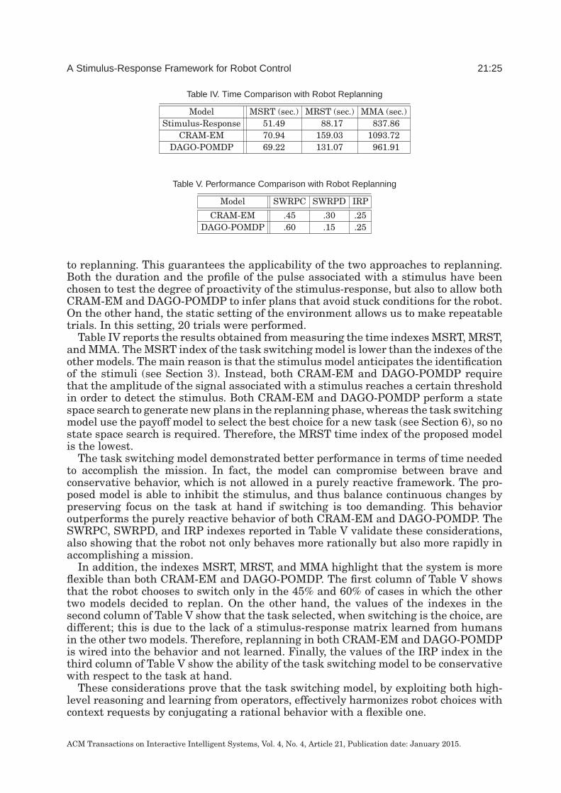
A Stimulus-Response Framework for Robot Control 21:25
Table IV. Time Comparison with Robot Replanning
Model MSRT (sec.) MRST (sec.) MMA (sec.)Stimulus-Response 51.49 88.17 837.86
CRAM-EM 70.94 159.03 1093.72DAGO-POMDP 69.22 131.07 961.91
Table V. Performance Comparison with Robot Replanning
Model SWRPC SWRPD IRP
CRAM-EM .45 .30 .25DAGO-POMDP .60 .15 .25
to replanning. This guarantees the applicability of the two approaches to replanning.Both the duration and the profile of the pulse associated with a stimulus have beenchosen to test the degree of proactivity of the stimulus-response, but also to allow bothCRAM-EM and DAGO-POMDP to infer plans that avoid stuck conditions for the robot.On the other hand, the static setting of the environment allows us to make repeatabletrials. In this setting, 20 trials were performed.
Table IV reports the results obtained from measuring the time indexes MSRT, MRST,and MMA. The MSRT index of the task switching model is lower than the indexes of theother models. The main reason is that the stimulus model anticipates the identificationof the stimuli (see Section 3). Instead, both CRAM-EM and DAGO-POMDP requirethat the amplitude of the signal associated with a stimulus reaches a certain thresholdin order to detect the stimulus. Both CRAM-EM and DAGO-POMDP perform a statespace search to generate new plans in the replanning phase, whereas the task switchingmodel use the payoff model to select the best choice for a new task (see Section 6), so nostate space search is required. Therefore, the MRST time index of the proposed modelis the lowest.
The task switching model demonstrated better performance in terms of time neededto accomplish the mission. In fact, the model can compromise between brave andconservative behavior, which is not allowed in a purely reactive framework. The pro-posed model is able to inhibit the stimulus, and thus balance continuous changes bypreserving focus on the task at hand if switching is too demanding. This behavioroutperforms the purely reactive behavior of both CRAM-EM and DAGO-POMDP. TheSWRPC, SWRPD, and IRP indexes reported in Table V validate these considerations,also showing that the robot not only behaves more rationally but also more rapidly inaccomplishing a mission.
In addition, the indexes MSRT, MRST, and MMA highlight that the system is moreflexible than both CRAM-EM and DAGO-POMDP. The first column of Table V showsthat the robot chooses to switch only in the 45% and 60% of cases in which the othertwo models decided to replan. On the other hand, the values of the indexes in thesecond column of Table V show that the task selected, when switching is the choice, aredifferent; this is due to the lack of a stimulus-response matrix learned from humansin the other two models. Therefore, replanning in both CRAM-EM and DAGO-POMDPis wired into the behavior and not learned. Finally, the values of the IRP index in thethird column of Table V show the ability of the task switching model to be conservativewith respect to the task at hand.
These considerations prove that the task switching model, by exploiting both high-level reasoning and learning from operators, effectively harmonizes robot choices withcontext requests by conjugating a rational behavior with a flexible one.
ACM Transactions on Interactive Intelligent Systems, Vol. 4, No. 4, Article 21, Publication date: January 2015.

21:26 M. Gianni et al.
8. CONCLUSION
In this work, we proposed a model for robot stimuli and stimulus-response that cansignificantly improve robot control in general, and particularly in the robot’s interactionwith the environment. The proposed approach indicates a new way to address robotcognitive control by showing that interaction with the environment can be proactive ifstimuli are taken into account not individually but as a whole system whose specificaspects can be learned by interacting with human users. This gained flexibility inrobot control can increase the usability of the robot, especially for operators who haveto deal with it in extreme environments like first-responder training areas or evenpost-disaster environments.
Our approach is completely novel, and, to our knowledge, no other approach to robotcognitive control has developed these ideas. The proposed method is supported by afull implementation in an advanced robot platform endowed with multiple abilitiesto perform several tasks, in which the interplay with operators plays a crucial rolefor both learning and evaluating performance. Our approach is inspired by the widepsychophysical and psychological literature on human patterns in stimulus-responseand task-switching, although we have provided an integrated model that is tailored fora robot system and is replicable for other robotic platforms.
Only recently has the need to model the stimulus-response pattern leading to taskswitching and the cognitive functions of shifting and inhibition become a hot topic incognitive robotics [Medina Ayala et al. 2012; Nakano et al. 2011; Ganesh and Burdet2013; Ajoudani et al. 2013; Ding and Fang 2013; Tao et al. 2012; Li et al. 2013; Sunget al. 2013; Jamone et al. 2013; Saglam and Byl 2013; and Li and Cheah 2012]. Theearliest studies were carried out within brain-actuated interaction [Milln et al. 2004],mechatronics [Capi 2007], behavior learning [Ito et al. 2006], navigation [Althaus andChristensen 2003], and planning [Finzi and Pirri 2005]. Recently, several studiesposited the need to model task switching to cope with adaptivity and ecological be-haviors in a dynamic environment [Capi et al. 2008; Suzuki et al. 2009; Wawerla andVaughan 2009; Durkee et al. 2011; D’Ambrosio et al. 2011].
In building the stimulus model, the main difficulties we encountered were due tothe experimental setting and data collection from several operators. This led us toprovide an outliers rejection method specifically for the stimuli; this method supportsthe selection of the training set on the basis of the features manifold eliciting thestimuli. This turned out to be a good solution to transfer training data acquired byhuman operators to the robot training set. To learn the stimulus-response selection,we still used several operators, but to infer unknown data we use low-rank matrixfactorization methods [Zhang et al. 2012; Chen 2008; Buchanan and Fitzgibbon 2005;Canny 2002] widely employed in recommendation systems and collaborative filtering[Ko and Lee 2002; L. Herlocker et al. 2004]). This model has proved suitable to estimatethe latent parameters underlying stimulus-response mapping, as well as to predict theweights given by each stimulus to each response, which are missing in the observeddata.
The problem of shifting and inhibition induced by stimuli was modeled by a switchingcost, obtained by conjugating a cost to reconfigure the robot state for the new goal andthe cost to resolve interference with the current activities set. Finally, the decisionproblem culminates in the definition of the payoff for switching, which requires us toconsider the risk and effort in computing the cost. We used time to failure to combinethe whole effort and predict the reliability of all the decision components to calculatethe payoff for switching.
We also introduced a connection between stimuli and reasoning level by defining aboundary shared by the two levels via the mapping E that plays the role of transduction,lifting the terms from the sample space of features, where yields are sampled, to the
ACM Transactions on Interactive Intelligent Systems, Vol. 4, No. 4, Article 21, Publication date: January 2015.

A Stimulus-Response Framework for Robot Control 21:27
terms of the language. Thus, logical inference provides the grounds for the causal andconstraint relations among processes carrying the information driven by stimuli. Thelogical structure is also the framework within which both processes and the robot’smental states can be defined, and it is where the reconfiguration and interference costscan be fully interpreted.
The proposed method improves both autonomy and flexibility in robot control. Fur-thermore, according to the experiments done to verify the coherence and rationalityof robot behaviors with respect to operator behavior while teleoperating the robot, theapproach proves to be very promising for improving the proactive interactions with theenvironment required by a robot relating to people and their needs.
Comparing the proposed framework with two other approaches to robot replanning,both robot flexibility and performance, in terms of time and tasks choices, are improved.It follows that robot usability also is improved since user stress can be reduced bylimiting the workload that continuous monitoring of robot activities demands of theoperator.
A. APPENDIX: IMPLEMENTATION
A.1. Hardware Description
The robotic platform is designed for harsh, unmanned environments. These are large-scale environments where robot missions last for long time periods and several eventsand stimuli burden the robot’s exploration and reporting activities.
The robot platform c©BlueBotics, named Absolem, has a central body where the elec-tronics is located and has two bogies on the sides. Each bogie is made of a central trackfor locomotion and two active flippers on both ends to extend the climbing capabilities.A breakable passive differential system allows the rotation of the bogies around thebody. Several sensors are installed on the platform, among them a rotating 2D laserscanner, an omnidirectional camera with a 360-degree field of view, an IMU/GPS, anda panoramic microphone.
A.2. Low-Level Robot Functionalities
The robot’s Simultaneous Localization and Mapping (SLAM) is based on a real-time3D ICP [Pomerleau et al. 2013]. A Dead Reckoning Navigation System (DRNS), basedon a Complementary Filter (CF), estimates the Euler angles of the robot body fromthe fusion of both odometry and the IMU inertial data [Cao et al. 2009; Kubelka andReinstein 2012]. Both ICP-based SLAM and DRNS provide, at real-time, the pose ofthe robot as a feedback to the Trajectory Tracking Controller (TTC) [Gianni et al.2013b]. Static traversability cost assessment of the ground, from point cloud data, isperformed by both physics-based terrain [Stoyanov et al. 2010; Papadakis and Pirri2012] and physical constraints analysis [Cafaro et al. 2013]. Visual perception of theenvironment is limited to object (e.g., signs, cars, and persons) detection accomplishedwith an omnidirectional camera [Hurych et al. 2011].
A.3. Robot Model
The robot model provides a representation of both the hardware and software com-ponents and of the processes activated by each component. For example, the SLAMsoftware module is modeled as a component, whereas the mapping and localiza-tion functionalities are represented as processes managed by the SLAM component.Table VI lists the main components and processes of the robot system model. Here, by
ACM Transactions on Interactive Intelligent Systems, Vol. 4, No. 4, Article 21, Publication date: January 2015.

21:28 M. Gianni et al.
Table VI. Components and Processes of the Robot Model
Component Id Component Description Process Id Process Description
C1 Battery π1,C1 Power Level MonitoringC2 WiFi π1,C2 Connection Management
C3
π1,C3 ROS Drivers Running3D Laser Scan π2,C3 Laser Rotating
π3,C3 Scanning
C4
π1,C4 ROS Packages RunningSLAM π2,C4 2D Mapping
π3,C4 3D Mappingπ4,C4 Localizing
C5
π1,C5 ROS Drivers RunningVision System π2,C5 Calibrating
π3,C5 Streaming
C6
π1,C6 ROS Packages RunningVisual Perception π2,C6 Detecting Object/Person
π3,C6 Recognizing Object/Person
C7
π1,C7 ROS Drivers RunningRobot Engine π2,C7 Locomotion System Monitoring
π3,C7 Temperature Monitoringπ4,C7 Locking Differential Drive
C8
π1,C8 ROS Packages RunningTrajectory Control π2,C8 Planning
π3,C8 Tracking
C9Dialogue π1,C9 Human to Robot Exchanging msg
π2,C9 Robot to Human Exchanging msg
C10
π1,C10 ROS Drivers RunningMicrophone π2,C10 Hearing
π3,C10 Speech Recognizing
C11
π1,C11 Data ReadingMemory π2,C11 Data Writing
π3,C11 Memory Checking
C12IMU π1,C12 ROS Drivers Running
π2,C12 Robot Pose EstimatingC13 ROS Master Core π1,C13 ROS Core Running
C14Central Processing Unit π1,C14 Payload Monitoring
π2,C14 Temperature Monitoring
C15
π1,C15 ROS Packages Runningπ2,C15 Traversability Analysis
Terrain Analysis π3,C15 Ground Subtracting & Analysisπ4,C15 Obstacle Detectingπ5,C15 Adapting Robot Morphology
C16Diagnostic π1,C16 System Check
π2,C16 Repair
Ck we denote the k-th robot component and by π j,Ck the j-th process managed by thek-th component.
A set of robot processes defines a task. This set of tasks forms the robot task library.For example, the task to overcome an obstacle requires that all the processes managedby the 3D Laser Scan component are active, that the 3D mapping process is running,and that the process adapting robot morphology to the terrain provides the correct
ACM Transactions on Interactive Intelligent Systems, Vol. 4, No. 4, Article 21, Publication date: January 2015.

A Stimulus-Response Framework for Robot Control 21:29
positions for the flippers. Table VII lists the set of tasks designed in agreement withthe available robot functionalities. Here, by τi we denote the i-th task in the task library.The right column in Table VII lists all the processes that need to be activated for therobot to perform the corresponding task.
Each process yields a quantum of information with characteristic features. Thisquantum of information is called the yield of the process. For example, the processmonitoring the temperature of the robot engine outputs, over time, the servo-motorstemperature. The information carried by the processes regulates the robot’s behaviors.For example, the engine temperature could reach a critical level and damage the robotservo-motors. The critical engine temperature level, as well as the loss of the WiFiconnection between the robot and the remote command post, are stimuli, and they areidentified from the process yields. Table VIII lists a description for each robot stimuli.Note that each process can trigger a single stimulus; therefore, the number and typesof stimuli are determined by the number and types of processes and these, in turn, aredetermined by the number and types of robot components. In the table, the term yπ j,Ck
denotes the stimulus triggered by the yield of the j-th process managed by the k-thcomponent Ck.
A.4. Robot Control
Robot control is defined by a declarative temporal model of its activities and a planningengine. The declarative temporal model is specified in the Temporal Flexible SituationCalculus (TFSC) [Finzi and Pirri 2005; Carbone et al. 2008] so that the main com-ponents and processes of the robot system reported in Table VI are represented bycause-effect relationships as well as by the temporal and spatial constraints amongthe processes [Pirri and Reiter 2000; Finzi and Pirri 2005], as discussed in Section 5.Planning is composed of two main logical modules: the plan generator and the execu-tion monitoring. The plan generator relies on a library of Prolog scripts that designatesthe set of tasks (see Table VII) that the robot can perform according to the speci-fied processes, their temporal constraints (compatibilities), and their preconditions.Execution-monitoring is a continuous process ensuring that both the set of action se-quences generated by the plan generator according to the TFSC model and the currentstate of the domain knowledge are consistently executed. The execution monitoring em-beds the model of task switching to regulate the behavior of the robot in responses tothe incoming stimuli. Both the TFSC model and the planning engine are implementedin Eclipse Prolog [Apt 2006], which optimally combines the power of a constraint solver(for time and compatibility constraints) with inference in order to generate the set ofaction sequences and also to enable continuous updates from incoming new knowledgeby using finite regression [Pirri and Reiter 2000].
The distributed working memory structure interconnects the TFSC model and theplanning engine with the task switching engine and with the robot functionalitiesthat are integrated in the ROS Operating System (ROS) [Quigley et al. 2009] (seeFigure 10). The structure is distributed over a collection of ROS services, organized asa set of addressable memory registers. In addition to the usual reading and writingoperations, the structure provides additional operations like memory dumping andupdate acknowledgment operations, suitable to check both consistency and persistenceof the state of the memory. The working memory system also takes care of mapping theinternal state of the robot into a representation suitable for planning and reasoningabout tasks.
The overall robot control provides bidirectional communication interfaces withthe human user. It further allows the human operator to switch between several
ACM Transactions on Interactive Intelligent Systems, Vol. 4, No. 4, Article 21, Publication date: January 2015.

21:30 M. Gianni et al.
Tabl
eV
II.Ta
skS
tate
s
Tas
kId
Tas
kD
escr
ipti
onP
roce
sses
τ 1R
obot
Sys
tem
Rec
over
y{π
1,C
16,π
2,C
16}
τ 2R
equ
est
for
Pat
hto
the
Ope
rato
r{π
1,C
2,π
1,C
4,π
3,C
4,π
1,C
7,π
1,C
9,π
1,C
13,π
1,C
15,π
3,C
15,π
4,C
15}
τ 3T
rack
Tra
ject
ory
⎧ ⎪ ⎨ ⎪ ⎩π1,
C1,π
1,C
2,π
1,C
3,π
2,C
3,π
3,C
3,π
1,C
4,π
3,C
4,π
4,C
4,π
1,C
5,π
3,C
5,
π1,
C6,π
2,C
6,π
1,C
7,π
2,C
7,π
3,C
7,π
1,C
8,π
2,C
8,π
3,C
8,π
1,C
10,π
2,C
10,
π3,
C10
,π
3,C
11,π
1,C
12,π
2,C
12,π
1,C
13,π
1,C
14,π
2,C
14,π
1,C
15,π
2,C
15
⎫ ⎪ ⎬ ⎪ ⎭τ 4
Rec
over
yW
iFiS
ign
al
{ π1,
C1,π
1,C
4,π
4,C
4π
1,C
7,π
2,C
7,π
3,C
7,π
1,C
8,
π2,
C8,π
3,C
8,π
1,C
11,π
1,C
12,π
2,C
12,π
1,C
13,π
1,C
14,π
2,C
14
}τ 5
Ret
urn
toB
ase
{π1,
C1,π
1,C
4,π
4,C
4,π
1,C
7,π
2,C
7,π
1,C
8,π
2,C
8,π
3,C
8,π
1,C
11,π
1,C
12,π
2,C
12,π
1,C
13}
τ 6S
tore
Dat
a{π
2,C
11,π
1,C
13}
τ 7C
oolC
entr
alP
roce
ssin
gU
nit
{π1,
C1,π
1,C
2,π
1,C
3,π
1,C
4,π
1,C
5,π
1,C
7,π
1,C
10,π
1,C
12,π
1,C
13,π
1,C
14,}
τ 8L
abel
Map
{π1,
C2,π
1,C
5,π
3,C
5,π
1,C
6,π
3,C
6,π
2,C
9,π
2,C
11,π
1,C
13,π
1,C
15}
τ 9S
erve
Ope
rato
rR
equ
est
{ π1,
C2,π
1,C
3,π
1,C
4,π
1,C
5,π
1,C
7,π
2,C
7,π
3,C
7,π
2,C
9,π
1,C
10,
π2,
C10
,π
1,C
10,π
2,C
11,π
1,C
12,π
1,C
13,π
1,C
14,π
2,C
14,π
1,C
15
}
τ 10
App
roac
hO
bjec
t/P
erso
n/S
oun
dS
ourc
e
⎧ ⎪ ⎨ ⎪ ⎩π1,
C1,π
1,C
2,π
1,C
3,π
2,C
3,π
3,C
3,π
1,C
4,π
2,C
4,π
3,C
4,π
4,C
4,π
1,C
5,
π3,
C5,π
1,C
6,π
1,C
7,π
2,C
7,π
3,C
7,π
1,C
8,π
2,C
8,π
3,C
8,π
2,C
11,π
1,C
12,
π2,
C12
,π
1,C
13,π
1,C
14,π
2,C
14,π
1,C
15,π
2,C
15,π
4,C
15,π
5,C
15
⎫ ⎪ ⎬ ⎪ ⎭τ 1
1O
verc
ome
Obs
tacl
e{π
1,C
3,π
2,C
3,π
3,C
3,π
1,C
4,π
3,C
4,π
1,C
7,π
2,C
7,π
3,C
7,π
4,C
7,π
1,C
13.π
1,C
15,π
5,C
15}
τ 12
Dat
aR
etri
eval
{π1,
C2,π
1,C
11,π
1,C
13}
τ 13
Rob
otS
yste
mR
econ
figu
rati
on{π
1,C
3,π
1,C
5,π
2,C
5,π
1,C
7,π
1,C
10,π
1,C
12,π
1,C
13,π
2,C
16}
ACM Transactions on Interactive Intelligent Systems, Vol. 4, No. 4, Article 21, Publication date: January 2015.
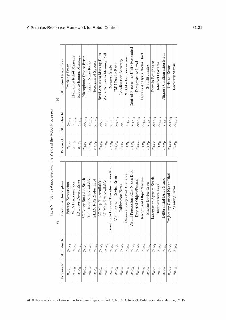
A Stimulus-Response Framework for Robot Control 21:31
Tabl
eV
III.S
timul
iAss
ocia
ted
with
the
Yie
lds
ofth
eR
obot
Pro
cess
es
(a)
(b)
Pro
cess
IdS
tim
ulu
sId
Sti
mu
lus
Des
crip
tion
π1,
C1
y π1,
C1
Bat
tery
Exh
aust
ion
π1,
C2
y π1,
C2
WiF
iDis
con
nec
tion
π1,
C3
y π1,
C3
3DL
aser
Dev
ice
Err
orπ
2,C
3y π
2,C
33D
Las
erR
otat
ion
Stu
ckπ
3,C
3y π
3,C
3S
can
Dat
aN
otA
vail
able
π1,
C4
y π1,
C4
SL
AM
RO
SN
odes
Die
dπ
2,C
4y π
2,C
42D
Map
Not
Ava
ilab
leπ
3,C
4y π
3,C
43D
Map
Not
Ava
ilab
leπ
4,C
4y π
4,C
4C
oord
inat
eF
ram
esT
ran
sfor
mat
ion
Err
orπ
1,C
5y π
1,C
5V
isio
nS
yste
mD
evic
eE
rror
π2,
C5
y π2,
C5
Cal
ibra
tion
Err
orπ
3,C
5y π
3,C
5C
amer
aIm
ages
Not
Ava
ilab
leπ
1,C
6y π
1,C
6V
isu
alP
erce
ptio
nR
OS
Nod
esD
ied
π2,
C6
y π2,
C6
Det
ecte
dO
bjec
t/P
erso
nπ
3,C
6y π
3,C
6R
ecog
niz
edO
bjec
t/P
erso
nπ
1,C
7y π
1,C
7E
ngi
ne
Dev
ice
Err
orπ
2,C
7y π
2,C
7L
ocom
otio
nS
yste
mS
tuck
π3,
C7
y π3,
C7
Tem
pera
ture
Lev
elπ
4,C
7y π
4,C
7D
iffe
ren
tial
Dri
veS
tuck
π1,
C8
y π1,
C8
Tra
ject
ory
Con
trol
Nod
esD
ied
π2,
C8
y π2,
C8
Pla
nn
ing
Err
or
Pro
cess
IdS
tim
ulu
sId
Sti
mu
lus
Des
crip
tion
π3,
C8
y π3,
C8
Tra
ckin
gE
rror
π1,
C9
y π1,
C9
Hu
man
toR
obot
Mes
sage
π2,
C9
y π2,
C9
Rob
otto
Hu
man
Mes
sage
π1,
C10
y π1,
C10
Mic
roph
one
Dev
ice
Err
orπ
2,C
10y π
2,C
10S
ign
alN
oise
Rat
ioπ
3,C
10y π
3,C
10R
ecog
niz
edS
peec
hπ
1,C
11y π
1,C
11R
ead
Acc
ess
toM
issi
ng
Dat
aπ
2,C
11y π
2,C
11W
rite
Acc
ess
toM
emor
yF
ull
π3,
C11
y π3,
C11
Mem
ory
Sta
teπ
1,C
12y π
1,C
12IM
UD
evic
eE
rror
π2,
C12
y π2,
C12
Loc
aliz
atio
nA
ccu
racy
π1,
C13
y π1,
C13
RO
SM
aste
rC
onn
ecti
onπ
1,C
14y π
1,C
14C
entr
alP
roce
ssin
gU
nit
Ove
rloa
ded
π2,
C14
y π2,
C14
Tem
pera
ture
Lev
elπ
1,C
15y π
1,C
15T
erra
inA
nal
ysis
Nod
esD
ied
π2,
C15
y π2,
C15
Sta
bili
tyIn
dex
π3,
C15
y π3,
C15
Ter
rain
Rou
ghn
ess
π4,
C15
y π4,
C15
Det
ecte
dO
bsta
cle
π5,
C15
y π5,
C15
Fli
pper
sC
onfi
gura
tion
Err
orπ
1,C
16y π
1,C
16C
riti
calE
rror
π2,
C16
y π2,
C16
Rec
over
yS
tatu
s
ACM Transactions on Interactive Intelligent Systems, Vol. 4, No. 4, Article 21, Publication date: January 2015.
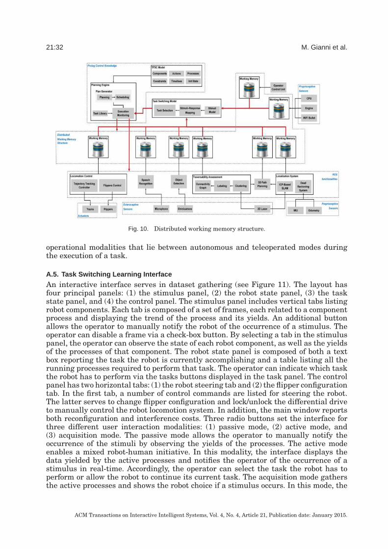
21:32 M. Gianni et al.
Fig. 10. Distributed working memory structure.
operational modalities that lie between autonomous and teleoperated modes duringthe execution of a task.
A.5. Task Switching Learning Interface
An interactive interface serves in dataset gathering (see Figure 11). The layout hasfour principal panels: (1) the stimulus panel, (2) the robot state panel, (3) the taskstate panel, and (4) the control panel. The stimulus panel includes vertical tabs listingrobot components. Each tab is composed of a set of frames, each related to a componentprocess and displaying the trend of the process and its yields. An additional buttonallows the operator to manually notify the robot of the occurrence of a stimulus. Theoperator can disable a frame via a check-box button. By selecting a tab in the stimuluspanel, the operator can observe the state of each robot component, as well as the yieldsof the processes of that component. The robot state panel is composed of both a textbox reporting the task the robot is currently accomplishing and a table listing all therunning processes required to perform that task. The operator can indicate which taskthe robot has to perform via the tasks buttons displayed in the task panel. The controlpanel has two horizontal tabs: (1) the robot steering tab and (2) the flipper configurationtab. In the first tab, a number of control commands are listed for steering the robot.The latter serves to change flipper configuration and lock/unlock the differential driveto manually control the robot locomotion system. In addition, the main window reportsboth reconfiguration and interference costs. Three radio buttons set the interface forthree different user interaction modalities: (1) passive mode, (2) active mode, and(3) acquisition mode. The passive mode allows the operator to manually notify theoccurrence of the stimuli by observing the yields of the processes. The active modeenables a mixed robot-human initiative. In this modality, the interface displays thedata yielded by the active processes and notifies the operator of the occurrence of astimulus in real-time. Accordingly, the operator can select the task the robot has toperform or allow the robot to continue its current task. The acquisition mode gathersthe active processes and shows the robot choice if a stimulus occurs. In this mode, the
ACM Transactions on Interactive Intelligent Systems, Vol. 4, No. 4, Article 21, Publication date: January 2015.
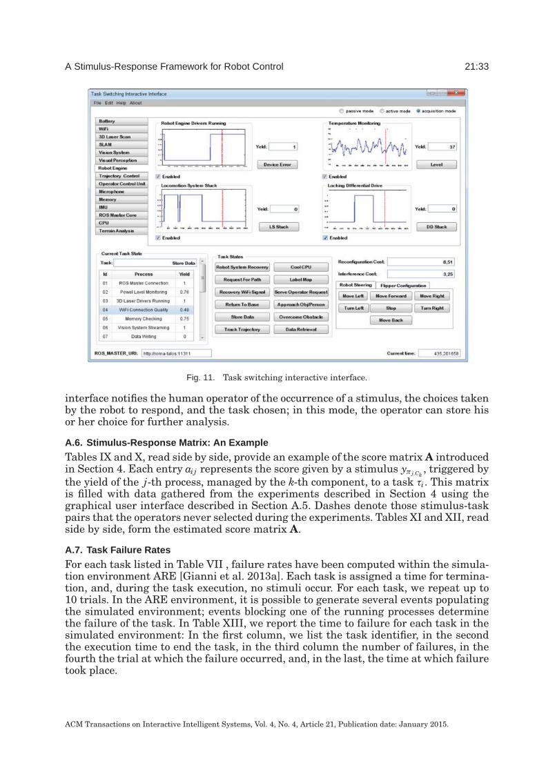
A Stimulus-Response Framework for Robot Control 21:33
Fig. 11. Task switching interactive interface.
interface notifies the human operator of the occurrence of a stimulus, the choices takenby the robot to respond, and the task chosen; in this mode, the operator can store hisor her choice for further analysis.
A.6. Stimulus-Response Matrix: An Example
Tables IX and X, read side by side, provide an example of the score matrix A introducedin Section 4. Each entry aij represents the score given by a stimulus yπ j,Ck
, triggered bythe yield of the j-th process, managed by the k-th component, to a task τi. This matrixis filled with data gathered from the experiments described in Section 4 using thegraphical user interface described in Section A.5. Dashes denote those stimulus-taskpairs that the operators never selected during the experiments. Tables XI and XII, readside by side, form the estimated score matrix A.
A.7. Task Failure Rates
For each task listed in Table VII , failure rates have been computed within the simula-tion environment ARE [Gianni et al. 2013a]. Each task is assigned a time for termina-tion, and, during the task execution, no stimuli occur. For each task, we repeat up to10 trials. In the ARE environment, it is possible to generate several events populatingthe simulated environment; events blocking one of the running processes determinethe failure of the task. In Table XIII, we report the time to failure for each task in thesimulated environment: In the first column, we list the task identifier, in the secondthe execution time to end the task, in the third column the number of failures, in thefourth the trial at which the failure occurred, and, in the last, the time at which failuretook place.
ACM Transactions on Interactive Intelligent Systems, Vol. 4, No. 4, Article 21, Publication date: January 2015.
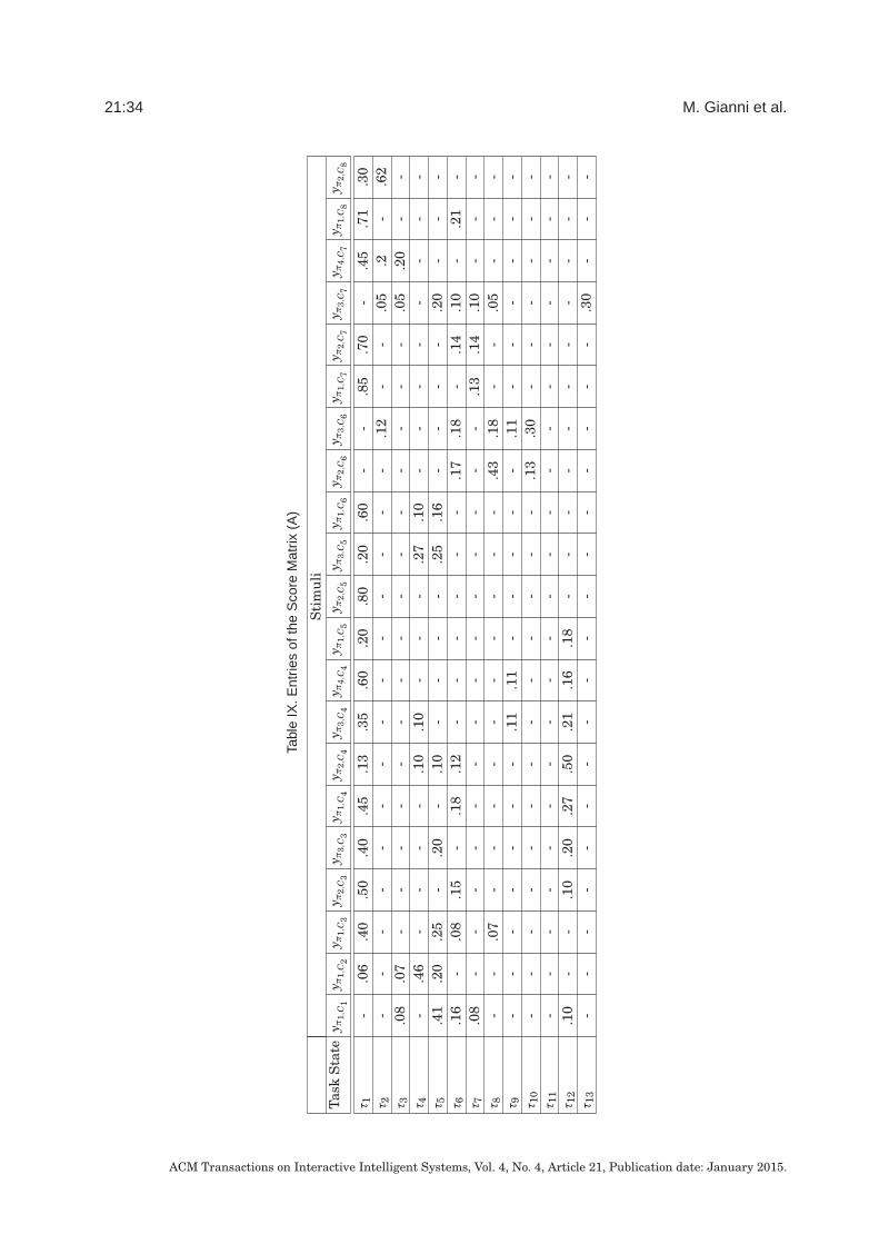
21:34 M. Gianni et al.
Tabl
eIX
.Ent
ries
ofth
eS
core
Mat
rix(A
)
Sti
mu
liT
ask
Sta
tey π
1,C
1y π
1,C
2y π
1,C
3y π
2,C
3y π
3,C
3y π
1,C
4y π
2,C
4y π
3,C
4y π
4,C
4y π
1,C
5y π
2,C
5y π
3,C
5y π
1,C
6y π
2,C
6y π
3,C
6y π
1,C
7y π
2,C
7y π
3,C
7y π
4,C
7y π
1,C
8y π
2,C
8
τ 1-
.06
.40
.50
.40
.45
.13
.35
.60
.20
.80
.20
.60
--
.85
.70
-.4
5.7
1.3
0τ 2
--
--
--
--
--
--
--
.12
--
.05
.2-
.62
τ 3.0
8.0
7-
--
--
--
--
--
--
--
.05
.20
--
τ 4-
.46
--
--
.10
.10
--
-.2
7.1
0-
--
--
--
-τ 5
.41
.20
.25
-.2
0-
.10
--
--
.25
.16
--
--
.20
--
-τ 6
.16
-.0
8.1
5-
.18
.12
--
--
--
.17
.18
-.1
4.1
0-
.21
-τ 7
.08
--
--
--
--
--
--
--
.13
.14
.10
--
-τ 8
--
.07
--
--
--
--
--
.43
.18
--
.05
--
-τ 9
--
--
--
-.1
1.1
1-
--
--
.11
--
--
--
τ 10
--
--
--
--
--
--
-.1
3.3
0-
--
--
-τ 1
1-
--
--
--
--
--
--
--
--
--
--
τ 12
.10
--
.10
.20
.27
.50
.21
.16
.18
--
--
--
--
--
-τ 1
3-
--
--
--
--
--
--
--
--
.30
--
-
ACM Transactions on Interactive Intelligent Systems, Vol. 4, No. 4, Article 21, Publication date: January 2015.

A Stimulus-Response Framework for Robot Control 21:35
Tabl
eX
.Ent
ries
ofth
eS
core
Mat
rix(B
)
Sti
mu
liT
ask
Sta
tey π
3,C
8y π
1,C
9y π
2,C
9y π
1,C
10y π
2,C
10y π
3,C
10y π
1,C
11y π
2,C
11y π
3,C
11y π
1,C
12y π
2,C
12y π
1,C
13y π
1,C
14y π
2,C
14y π
1,C
15y π
2,C
15y π
3,C
15y π
4,C
15y π
5,C
15y π
1,C
16y π
2,C
16
τ 1-
--
.25
.22
-.1
0.2
0-
.63
.14
.75
.38
.23
.33
--
-.3
7-
-τ 2
.61
-.6
6.1
2-
.10
--
.09
--
--
-.1
7.1
3-
.25
.12
--
τ 3.1
0.3
0-
.10
-.1
0-
-.0
8-
.42
--
-.1
6.2
0.4
3-
.12
--
τ 4-
--
--
-.1
0-
--
--
--
--
--
--
-τ 5
.10
--
--
-.2
0.2
0.1
1-
.14
-.1
6-
.16
.12
.28
.08
.12
-.7
8τ 6
-.0
7-
--
.12
.55
-.6
2-
--
.08
.23
.15
--
--
--
τ 7-
--
--
--
--
--
-.0
8.3
8-
--
--
--
τ 8-
-.2
2.1
1-
.12
--
--
--
--
--
-.2
5-
--
τ 9-
.39
.10
.12
.19
.22
--
--
--
.08
--
--
--
--
τ 10
.12
.16
-.1
2.4
5.3
0-
--
-.1
4-
--
-.3
7.1
4-
.12
--
τ 11
--
--
--
--
--
.15
--
--
.10
.14
.25
--
-τ 1
2-
--
.12
--
-.5
5-
.09
--
--
--
--
.13
--
τ 13
--
--
--
--
--
--
--
--
--
-.7
4-
ACM Transactions on Interactive Intelligent Systems, Vol. 4, No. 4, Article 21, Publication date: January 2015.

21:36 M. Gianni et al.
Tabl
eX
I.C
ompl
eted
Sco
reM
atrix
(A)
Sti
mu
liT
ask
Sta
tey π
1,C
1y π
1,C
2y π
1,C
3y π
2,C
3y π
3,C
3y π
1,C
4y π
2,C
4y π
3,C
4y π
4,C
4y π
1,C
5y π
2,C
5y π
3,C
5y π
1,C
6y π
2,C
6y π
3,C
6y π
1,C
7y π
2,C
7y π
3,C
7y π
4,C
7y π
1,C
8y π
2,C
8
τ 1.0
4.1
5.3
9.4
9.4
1.4
4.1
3.3
5.6
0.2
0.7
9.2
1.6
1.0
1.0
2.8
4.7
2.0
4.4
5.7
1.3
0τ 2
.02
.02
.03
.02
.01
.01
.01
.03
.01
.05
.02
.01
.01
.01
.12
.01
.01
.03
.20
.01
.62
τ 3.0
8.0
7.0
1.0
3.0
1.0
1.0
1.0
1.0
1.0
5.0
2.0
2.0
2.0
1.0
1.0
1.0
2.0
5.2
0.0
1.0
1τ 4
.02
.45
.02
.04
.02
.01
.10
.10
.01
.05
.02
.26
.10
.02
.01
.01
.00
.03
.02
.01
.01
τ 5.4
2.2
0.2
4.0
2.2
0.0
1.1
0.0
3.0
1.0
5.0
2.2
4.1
3.0
2.0
1.0
1.0
0.1
9.0
1.0
1.0
1τ 6
.17
.01
.09
.15
.02
.19
.10
.01
.01
.06
.02
.04
.03
.17
.17
.01
.13
.11
.01
.21
.01
τ 7.0
8.0
2.0
1.0
2.0
1.0
1.0
1.0
3.0
1.0
6.0
2.0
1.0
1.0
3.0
1.1
3.1
5.1
0.0
1.0
1.0
1τ 8
.02
.01
.07
.02
.02
.01
.01
.01
.01
.06
.02
.02
.01
.43
.17
.00
.01
.05
.01
.01
.01
τ 9.0
2.0
1.0
2.0
2.0
2.0
1.0
1.1
1.1
1.0
5.0
2.0
1.0
1.0
2.1
2.0
1.0
1.0
2.0
2.0
1.0
1τ 1
0.0
2.0
1.0
2.0
2.0
2.0
1.0
1.0
2.0
3.0
5.0
2.0
2.0
2.1
3.2
9.0
1.0
0.0
3.0
2.0
1.0
1τ 1
1.0
2.0
1.0
2.0
1.0
1.0
2.0
1.0
3.0
1.0
5.0
2.0
3.0
2.0
2.0
1.0
1.0
1.0
2.0
4.0
1.0
1τ 1
2.1
0.0
1.0
2.1
1.2
0.2
6.4
8.2
0.1
4.1
8.0
2.0
1.0
1.0
2.0
6.0
0.0
2.0
1.0
1.0
1.0
1τ 1
3.0
1.0
3.0
6.0
5.0
5.0
4.0
2.0
7.0
4.0
8.0
2.1
1.0
2.1
1.0
2.0
1.0
1.3
0.0
3.0
1.0
1
ACM Transactions on Interactive Intelligent Systems, Vol. 4, No. 4, Article 21, Publication date: January 2015.

A Stimulus-Response Framework for Robot Control 21:37
Tabl
eX
II.C
ompl
eted
Sco
reM
atrix
(B)
Sti
mu
liT
ask
Sta
tey π
3,C
8y π
1,C
9y π
2,C
9y π
1,C
10y π
2,C
10y π
3,C
10y π
1,C
11y π
2,C
11y π
3,C
11y π
1,C
12y π
2,C
12y π
1,C
13y π
1,C
14y π
2,C
14y π
1,C
15y π
2,C
15y π
3,C
15y π
4,C
15y π
5,C
15y π
1,C
16y π
2,C
16
τ 1.0
08.0
1.0
04.2
40.2
10.0
05.1
00.2
00.0
12.6
10.1
40.7
50.3
70.2
20.3
30.0
09.0
01.0
18.3
70.0
20.0
16τ 2
.600
.005
.670
.110
.010
.110
.007
.005
.090
.044
.001
.020
.014
.015
.170
.130
.001
.250
.120
.024
.020
τ 3.1
10.2
90.0
02.1
20.0
22.0
90.0
03.0
09.0
80.0
26.3
90.0
30.0
02.0
17.1
60.2
00.4
30.0
17.1
20.0
21.0
15τ 4
.006
.020
.001
.005
.008
.006
.100
.005
.010
.021
.001
.050
.004
.013
.004
.011
.001
.019
.003
.020
.049
τ 5.1
20.0
07.0
02.0
15.0
10.0
04.1
90.2
00.1
20.0
29.1
40.0
10.1
60.0
19.1
70.1
20.2
80.0
80.1
20.0
33.7
50τ 6
.007
.070
.001
.013
.005
.110
.560
.001
.610
.030
.001
.020
.080
.230
.150
.010
.001
.015
.001
.021
.019
τ 7.0
05.0
07.0
02.0
07.0
15.0
15.0
10.0
07.0
11.0
20.0
03.0
30.0
80.3
80.0
04.0
10.0
01.0
21.0
03.0
21.0
21τ 8
.007
.009
.210
.110
.010
.110
.004
.003
.012
.025
.001
.020
.002
.015
.003
.013
.001
.250
.004
.022
.018
τ 9.0
09.3
80.1
00.1
30.2
00.2
30.0
05.0
04.0
10.0
30.0
01.0
20.0
80.0
16.0
03.0
07.0
01.0
26.0
02.0
21.0
19τ 1
0.1
00.1
70.0
02.1
10.4
40.2
90.0
06.0
06.0
12.0
27.1
40.0
30.0
03.0
17.0
05.3
70.1
40.0
17.1
20.0
24.0
16τ 1
1.0
08.0
09.0
03.0
08.0
10.0
10.0
03.0
07.0
11.0
23.1
50.0
10.0
02.0
16.0
04.1
00.1
40.2
50.0
04.0
21.0
20τ 1
2.0
06.0
07.0
02.1
20.0
10.0
17.0
05.5
50.0
09.0
90.0
01.0
20.0
02.0
14.0
03.0
15.0
01.0
19.1
30.0
23.0
18τ 1
3.0
14.0
16.0
01.0
12.0
50.0
03.0
07.0
03.0
13.0
25.0
01.0
20.0
03.0
18.0
04.0
05.0
01.0
18.0
03.7
10.0
19
ACM Transactions on Interactive Intelligent Systems, Vol. 4, No. 4, Article 21, Publication date: January 2015.

21:38 M. Gianni et al.
Table XIII. Task Time to Failure
Task Id Execution Time (min.) # of Failures Failure time (min.)
τ1 18 0 - -τ2 16 1 Trial 3 15.23
τ3 46 4
Trial 2 12.51Trial 3 28.09Trial 6 31.11Trial 9 5.06
τ4
Trial 4 19.0131 3 Trial 7 18.75
Trial 6 19.23
τ5 82 4
Trial 1 10.91Trial 2 40.05Trial 4 19.32
Trial 10 47.09τ6 25 1 Trial 8 7.51τ7 27 0 - -
τ855 2 Trial 1 39.41
Trial 8 38.02
τ9
Trial 2 28.9146 3 Trial 3 29.78
Trial 9 20.03
τ10
Trial 1 12.01100 4 Trial 3 27.09
Trial 8 81.53Trial 9 82.09
τ11
Trial 5 51.7968 3 Trial 9 28.06
Trial 10 31.55
τ1239 2 Trial 1 11.77
Trial 7 12.33
τ13
Trial 5 39.6048 3 Trial 6 40.79
Trial 10 26.56
ACKNOWLEDGMENTS
We also thank reviewers for their thorough advices in improving this article.
REFERENCES
A. Ajoudani, M. Gabiccini, N. G. Tsagarakis, and A. Bicchi. 2013. Human-like impedance and minimum effortcontrol for natural and efficient manipulation. In Proceedings of the IEEE International Conference onRobotics and Automation. 4499–4505.
J. F. Allen. 1983. Maintaining knowledge about temporal intervals. Communications of the ACM 26, 11(1983), 832–843.
P. Althaus and H. I. Christensen. 2003. Smooth task switching through behaviour competition. Robotics andAutonomous Systems 44, 3–4 (2003), 241–249.
K. Apt and M. Wallace. 2006. Constraint Logic Programming using Eclipse. Cambridge University Press,New York.
A. R. Aron. 2007. The neural basis of inhibition in cognitive control. The Neuroscientist 13 (2007), 214–228.T. Baar, B. Beckert, and P. H. Schmitt. 2001. An extension of dynamic logic for modelling ocls @pre operator.
In Perspectives of System Informatics, D. Bjrner, M. Broy, and A.V. Zamulin (Eds.). Lecture Notes inComputer Science, Vol. 2244. Springer, Berlin, 47–54.
ACM Transactions on Interactive Intelligent Systems, Vol. 4, No. 4, Article 21, Publication date: January 2015.

A Stimulus-Response Framework for Robot Control 21:39
M. Beetz, L. Mosenlechner, and M. Tenorth. 2010. CRAM: A cognitive robot abstract machine for everydaymanipulation in human environments. In Proceedings of the IEEE/RSJ International Conference onIntelligent Robots and Systems. 1012–1017.
S. A. Block, A. F. Wehowsky, and B. C. Williams. 2006. Robust execution on contingent, temporally flexibleplans. In Proceedings of the AAAI Workshop on Cognitive Robotics. AAAI Press, Palo Alto, California,802–808.
A. Blum and J. C. Langford. 1999. Probabilistic planning in the graphplan framework. In Proceedings of the5th European Conference on Planning. Springer-Verlag, New York, NY, 8–12.
A. M. Buchanan and A. W. Fitzgibbon. 2005. Damped newton algorithms for matrix factorization with missingdata. In Proceedings of the IEEE Conference on Computer Vision and Pattern Recognition. 316–322.
B. Cafaro, M. Gianni, F. Pirri, M. Ruiz, and A. Sinha. 2013. Terrain traversability in rescue environments.In Proceedings of the IEEE International Symposium on Safety, Security, and Rescue Robotics. 1–8.
J. F. Canny. 2002. Collaborative filtering with privacy via factor analysis. In Proceedings of the 25th AnnualInternational ACM SIGIR Conference on Research and Development in Information Retrieval. 238–245.
D. Cao, Q. Qu, C. Li, and C. He. 2009. Research of attitude estimation of UAV based on information fusionof complementary filter. In Proceedings of the 4th International Conference on Computer Sciences andConvergence Information Technology. IEEE, 1290–1293.
G. Capi. 2007. Robot task switching in complex environments. In Proceedings of the IEEE/ASME Interna-tional Conference on Advanced Intelligent Mechatronics. IEEE, 1–6.
G. Capi, G. G. Pojani, and S. I. Kaneko. 2008. Evolution of task switching behaviors in real mobile robots.In Proceedings of the 3rd International Conference on Innovative Computing Information and Control.IEEE, 495–501.
A. Carbone, A. Finzi, A. Orlandini, and F. Pirri. 2008. Model-based control architecture for attentive robotsin rescue scenarios. Autonomous Robots 24, 1 (2008), 87–120.
P. Chen. 2008. Optimization algorithms on subspaces: Revisiting missing data problem in low-rank matrix.International Journal of Computer Vision 80, 1 (2008), 125–142.
M. M. Cialdea and F. Pirri. 1993. First order abduction via tableau and sequent calculi. Logic Journal of theIGPL 1, 1 (1993), 99–117.
D. B. D’Ambrosio, J. Lehman, S. S. Risi, and K. O. Stanley. 2011. Task switching in multirobot learningthrough indirect encoding. In Proceedings of the IEEE/RSJ International Conference on IntelligentRobots and Systems. IEEE, 2802–2809.
R. Dechter, I. Meiri, and J. Pearl. 1991. Temporal constraint networks. Artificial Intelligence 49, 1–3 (1991),61–95.
X. Ding and C. Fang. 2013. A novel method of motion planning for an anthropomorphic arm based onmovement primitives. IEEE/ASME Transactions on Mechatronics 18, 2 (April 2013), 624–636.
K. T. Durkee, C. Shabarekh, C. Jackson, and G. Ganberg. 2011. Flexible autonomous support to aid contextand task switching. In Proceedings of the IEEE First International Multi-Disciplinary Conference onCognitive Methods in Situation Awareness and Decision Support. IEEE, 204–207.
R. Fikes and N. J. Nilsson. 1971. STRIPS: A new approach to the application of theorem proving to problemsolving. Artificial Intelligence 2, 3/4 (1971), 189–208.
M. Finger and D. Gabbay. 1996. Combining temporal logic systems. Notre Dame Journal of Formal Logic 37,2 (1996), 204–232.
A. Finzi and F. Pirri. 2005. Representing flexible temporal behaviours in the situation calculus. In Proceedingsof the 19th International Joint Conference on Artificial Intelligence. AAAI Press, 436–441.
A. Finzi and F. Pirri. 2010. Switching Tasks and Flexible Reasoning in the Situation Calculus. TechnicalReport 7. DIAG.
M. Fox and D. Long. 2003. PDDL2.1: An extension to PDDL for expressing temporal planning domains.Journal of Artificial Intelligence Research 20, 1 (2003), 61–124.
G. Ganesh and E. Burdet. 2013. Motor planning explains human behaviour in tasks with multiple solutions.Robotics and Autonomous Systems 61 (2013), 362–368. Issue 4.
M. Gianni, F. Ferri, and F. Pirri. 2013a. ARE: Augmented reality environment for mobile robots. In Proceed-ings of the 14th Towards Autonomous Systems (TAROS). 470–483.
M. Gianni, G. Gonnelli, A. Sinha, M. Menna, and F. Pirri. 2013b. An augmented reality approach for tra-jectory planning and control of tracked vehicles in rescue environments. In Proceedings of the IEEEInternational Symposium on Safety, Security, and Rescue Robotics. 1–6.
J. J. Gibson. 1960. The concept of the stimulus in psychology. American Psychologist 15, 11 (1960), 694–703.M. Gobelbecker, C. Gretton, and R. Dearden. 2011. A switching planner for combined task and observation
planning. In Proceedings of the 25th AAAI Conference on Artificial Intelligence.
ACM Transactions on Interactive Intelligent Systems, Vol. 4, No. 4, Article 21, Publication date: January 2015.

21:40 M. Gianni et al.
N. Hawes, M. Hanheide, K. Sjoo, A. Aydemir, P. Jensfelt, M. Gobelbecker, M. Brenner, H. Zender, P. Lison,I. Kruijff-Korbayova, G. J. M Kruijff, and M. Zillich. 2010. Dora the explorer: A motivated robot. InProceedings of 9th International Conference on Autonomous Agents and Multiagent Systems, Vol. 1.International Foundation for Autonomous Agents and Multiagent Systems, Canada, 1617–1618.
D. Hurych, K. Zimmermann, and T. Svoboda. 2011. Fast learnable object tracking and detection in high-resolution omnidirectional images. In Proceedings of the 9th International Joint Conference on ComputerVision, Imaging and Computer Graphics Theory and Applications. SCITEPRESS, 521–530.
M. Ito, K. Noda, Y. Hoshino, and J. Tani. 2006. Dynamic and interactive generation of object handlingbehaviors by a small humanoid robot using a dynamic neural network model. Neural Networks 19(2006), 323–337.
L. Jamone, B. Damas, J. Santos-Victor, and A. Takanishi. 2013. Online learning of humanoid robot kinematicsunder switching tools contexts. In Proceedings of the IEEE International Conference on Robotics andAutomation. 4811–4817.
A. T. Jersild. 1927. Mental set and shift. Archives of Psychology 14, 89 (1927), 5–82.S. Ko and J. Lee. 2002. User preference mining through collaborative filtering and content based filtering
in recommender system. In Proceedings of the 3rd International Conference on E-Commerce and WebTechnologies. 244–253.
V. Kubelka and M. Reinstein. 2012. Complementary filtering approach to orientation estimation usinginertial sensors only. In Proceedings of the IEEE International Conference on Robotics and Automation.599–605.
J. L. L. Herlocker, J. A. Konstan, L. G. Terveen, and J. T. T. Riedl. 2004. Evaluating collaborative filteringrecommender systems. ACM Transactions on Information Systems 22, 1 (2004), 5–53.
Tao Li, K. Nakajima, and R. Pfeifer. 2013. Online learning for behavior switching in a soft robotic arm. InProceedings of the IEEE International Conference on Robotics and Automation. 1296–1302.
X. Li and C. C. Cheah. 2012. Multiple task-space robot control: Sense locally, act globally. In Proceedings ofthe IEEE International Conference on Robotics and Automation. 265–270.
Pierre Marquis. 1991. Extending abduction from propositional to first-order logic. In Fundamentals of Arti-ficial Intelligence Research. 141–155.
D. V. McDermott. 2003. PDDL2.1 - The art of the possible? Commentary on Fox and Long. Journal of ArtificialIntelligence Research 20 (2003), 145–148.
A. I. Medina Ayala, S. B. Andersson, and C. Belta. 2012. Probabilistic control from time-bounded temporallogic specifications in dynamic environments. In Proceedings of the IEEE International Conference onRobotics and Automation. 4705–4710.
E. K. Miller and J. D. Cohen. 2007. An integrative theory of prefrontal cortex function. Annual Review ofNeuroscience 24 (2007), 167–202.
J. Milln, F. Renkens, J. Mourino, and W. Gerstner. 2004. Brain-actuated interaction. Artificial Intelligence159 (2004), 241–259.
S. Monsell. 2003. Task switching. Trends in Cognitive Sciences 7, 3 (2003), 134–140.P. H. Morris, N. Muscettola, and T. Vidal. 2001. Dynamic control of plans with temporal uncertainty. In
Proceedings of the 17th International Joint Conference on Artificial Intelligence. 494–502.M. Nakano, Y. Hasegawa, K. Funakoshi, J. Takeuchi, T. Torii, K. Nakadai, N. Kanda, K. Komatani, H. G
Okuno, and H. Tsujino. 2011. A multi-expert model for dialogue and behavior control of conversationalrobots and agents. Knowledge-Based Systems Journal 24 (2011), 248–256. Issue 2.
A. Newell. 1990. Unified Theories of Cognition. Harvard University Press.D. A. Norman and T. Shallice. 1986. Consciousness and Self-Regulation: Advances in Research and Theory,
Vol. 4. Attention to action: Willed and automatic control of behaviour. Plenum Press.P. Papadakis and F. Pirri. 2012. 3D mobility learning and regression of articulated, tracked robotic vehicles
by physics-based optimization. In Proceedings of the 9th Workshop on Virtual Reality Interactions andPhysical Simulations. 147–156.
F. Pirri. 2011. The well-designed logical robot: Learning and experience from observations to the SituationCalculus. Artificial Intelligence 175, 1 (2011), 378–415.
F. Pirri and R. Reiter. 1999. Some contributions to the metatheory of the situation calculus. Journal of theACM 46, 3 (1999), 325–361.
F. Pirri and R. Reiter. 2000. Planning with natural actions in the situation calculus. In Logic-Based ArtificialIntelligence. Kluwer Press, 213–231.
F. Pomerleau, F. Colas, S. Siegwart, and S. Magnenat. 2013. Comparing ICP variants on real-world data sets.Autonomous Robots 34, 3 (April 2013), 133–148.
ACM Transactions on Interactive Intelligent Systems, Vol. 4, No. 4, Article 21, Publication date: January 2015.
A Stimulus-Response Framework for Robot Control 21:41
M. Quigley, K. Conley, B. Gerkey, J. Faust, T. Foote, J. Leibs, R. Wheeler, and A. Ng. 2009. ROS: An open-sourceRobot Operating System. In Proceedings of the Open-Source Workshop of the International Conferenceon Robotics and Automation.
D. Randell, Z. Cui, and A. Cohn. 1992. A spatial logic based on regions and connection. In Proceedings of the3rd International Conference on Principles of Knowledge Representation and Reasoning. 165–176.
J. Rubinstein, D. E. Meyer, and J. E. Evans. 2001. Executive control of cognitive processes in task switching.Journal of Experimental Psychology: Human Perception and Performance 27, 4 (2001), 763–797.
C. O. Saglam and K. Byl. 2013. Stability and gait transition of the five-link biped on stochastically rough ter-rain using a discrete set of sliding mode controllers. In Proceedings of the IEEE International Conferenceon Robotics and Automation. 5675–5682.
T. Stoyanov, M. Magnusson, H. Andreasson, and A. J. Lilienthal. 2010. Path planning in 3D environmentsusing the Normal Distributions Transform. In Proceedings of the IEEE/RSJ International Conferenceon Intelligent Robots and Systems. 3263–3268.
C. Sung, N. Ayanian, and D. Rus. 2013. Improving the performance of multi-robot systems by task switching.In Proceedings of the IEEE International Conference on Robotics and Automation. 2999–3006.
S. Suzuki, T. Sasaki, and F. Harashima. 2009. Visible classification of task-switching strategies in vehicleoperation. In Proceedings of the 18th IEEE International Symposium on Robot and Human InteractiveCommunication. 1161–1166.
T. Takayuki Okatani and K. Deguchi. 2006. On the Wiberg algorithm for matrix factorization in the presenceof missing components. International Journal of Computer Vision 72, 3 (2006), 329–337.
K. Talamadupula, J. Benton, S. Kambhampati, P. Schermerhorn, and M. Scheutz. 2010. Planning for human-robot teaming in open worlds. ACM Transactions on Intelligent Systems and Technology 1, 2 (2010),14:1–14:24.
L. Tao, K. Nakajima, M. Cianchetti, C. Laschi, and R. Pfeifer. 2012. Behavior switching using reservoircomputing for a soft robotic arm. In Proceedings of the IEEE International Conference on Robotics andAutomation. 4918–4924.
S. P. Tipper. 2001. Does negative priming reflect inhibitory mechanisms? A review and integration of con-flicting views. The Quarterly Journal of Experimental Psychology 54 (2001), 321–343.
M. Vilain, H. Kautz, and P. Beek. 1986. Constraint propagation algorithms for temporal reasoning. InReadings in Qualitative Reasoning about Physical Systems. Morgan Kaufmann, 377–382.
J. Wawerla and R. T. Vaughan. 2009. Robot task switching under diminishing returns. In Proceedings of theIEEE/RSJ International Conference on Intelligent Robots and Systems. 5033–5038.
E. H. Weber. 1834. De pulsu, resorptione, audita et tactu. Annotationes anatomicae et physiologicae. Koehler,New York, NY.
J. Wittocx, M. Denecker, and M. Bruynooghe. 2010. Constraint propagation for extended first-order logic.Computing Research Repository abs/1008.2121 (2010).
F. Wolter and M. Zakharyaschev. 2000. Spatio-temporal representation and reasoning based on RCC-8. InProceedings of the 7th International Conference on Principles of Knowledge Representation and Reason-ing. 3–14.
J. L. Wyatt, A. Aydemir, M. Brenner, M. Hanheide, N. Hawes, P. Jensfelt, M. Kristan, G. J. M. Kruijff,P. Lison, A. Pronobis, K. Sjoo, A. Vrecko, H. Zender, M. Zillich, and D. Skocaj. 2010. Self-understandingand self-extension: A systems and representational approach. IEEE Transactions on Autonomous MentalDevelopment 2, 4 (2010), 282–303.
Z. Zhang, K. Zhao, and H. Zha. 2012. Inducible regularization for low-rank matrix factorizations for collab-orative filtering. Neurocomputing 97 (2012), 52–62.
Y. Zhou, D. M. Wilkinson, R. Schreiber, and R. Pan. 2008. Large-scale parallel collaborative filtering for thenetflix prize. In Proceedings of the 4th International Conference on Algorithmic Aspects in Informationand Management. 337–348.
Received February 2013; revised August 2014; accepted October 2014
ACM Transactions on Interactive Intelligent Systems, Vol. 4, No. 4, Article 21, Publication date: January 2015.