Download - The 1-D Heat Equation - École Polytechnique

The 1-D Heat Equation
18303 Linear Partial Differential Equations
Matthew J Hancock
Fall 2006
1 The 1-D Heat Equation
11 Physical derivation
Reference Guenther amp Lee sect13-14 Myint-U amp Debnath sect21 and sect25
[Sept 8 2006]
In a metal rod with non-uniform temperature heat (thermal energy) is transferred
from regions of higher temperature to regions of lower temperature Three physical
principles are used here
1 Heat (or thermal) energy of a body with uniform properties
Heat energy = cmu
where m is the body mass u is the temperature c is the specific heat units [c] =
L2Tminus2Uminus1 (basic units are M mass L length T time U temperature) c is the energy
required to raise a unit mass of the substance 1 unit in temperature
2 Fourierrsquos law of heat transfer rate of heat transfer proportional to negative
temperature gradient
Rate of heat transfer partu = (1) minusK0
area partx
where K0 is the thermal conductivity units [K0] = MLTminus3Uminus1 In other words heat
is transferred from areas of high temp to low temp
3 Conservation of energy
Consider a uniform rod of length l with non-uniform temperature lying on the
x-axis from x = 0 to x = l By uniform rod we mean the density ρ specific heat c
thermal conductivity K0 cross-sectional area A are ALL constant Assume the sides
1
of the rod are insulated and only the ends may be exposed Also assume there is no
heat source within the rod Consider an arbitrary thin slice of the rod of width Δx
between x and x+Δx The slice is so thin that the temperature throughout the slice
is u (x t) Thus
Heat energy of segment = c times ρAΔx times u = cρAΔxu (x t)
By conservation of energy
change of heat in from heat out from
heat energy of = left boundary
minus right boundary
segment in time Δt
From Fourierrsquos Law (1)
partu partu cρAΔxu (x t + Δt) minus cρAΔxu (x t) = ΔtA minusK0 minus ΔtA minusK0
partx partx x x+Δx
Rearranging yields (recall ρ c A K0 are constant)
u (x t + Δt) minusΔt
u (x t) =
K0
cρ
partu partx
x+Δx
minus Δx
partu partx
x
Taking the limit Δt Δx rarr 0 gives the Heat Equation
partu part2u
partt = κ
partx2 (2)
where
κ = K0
(3) cρ
is called the thermal diffusivity units [κ] = L2T Since the slice was chosen arbishy
trarily the Heat Equation (2) applies throughout the rod
12 Initial condition and boundary conditions
To make use of the Heat Equation we need more information
1 Initial Condition (IC) in this case the initial temperature distribution in the
rod u (x 0)
2 Boundary Conditions (BC) in this case the temperature of the rod is affected
by what happens at the ends x = 0 l What happens to the temperature at the
end of the rod must be specified In reality the BCs can be complicated Here we
consider three simple cases for the boundary at x = 0
2
(I) Temperature prescribed at a boundary For t gt 0
u (0 t) = u1 (t)
(II) Insulated boundary The heat flow can be prescribed at the boundaries
partu (0 t) = φ1 (t)minusK0
partx
(III) Mixed condition an equation involving u (0 t) partupartx (0 t) etc
Example 1 Consider a rod of length l with insulated sides is given an initial
temperature distribution of f (x) degree C for 0 lt x lt l Find u (x t) at subsequent
times t gt 0 if end of rod are kept at 0o C
The Heat Eqn and corresponding IC and BCs are thus
PDE ut = κuxx 0 lt x lt l (4)
IC u (x 0) = f (x) 0 lt x lt l (5)
BC u (0 t) = u (L t) = 0 t gt 0 (6)
Physical intuition we expect u 0 as t rarr infinrarr
13 Non-dimensionalization
Dimensional (or physical) terms in the PDE (2) k l x t u Others could be
introduced in IC and BCs To make the solution more meaningful and simpler we
group as many physical constants together as possible Let the characteristic length
time and temperature be Llowast Tlowast and Ulowast respectively with dimensions [Llowast] = L
[Tlowast] = T [Ulowast] = U Introduce dimensionless variables via
x t u (x t) f (x) x = t = ˆ ˆ t = x) = u x ˆ f (ˆ (7)
Llowast Tlowast Ulowast Ulowast
The variables x t u are dimensionless (ie no units [x] = 1) The sensible choice
for the characteristic length is Llowast = l the length of the rod While x is in the range
0 lt x lt l ˆ lt ˆx is in the range 0 x lt 1
The choice of dimensionless variables is an ART Sometimes the statement of the
problem gives hints eg the length l of the rod (1 is nicer to deal with than l an
unspecified quantity) Often you have to solve the problem first look at the solution
and try to simplify the notation
3
From the chain rule
partu partu partt Ulowast partuut = = Ulowast =
partt partt partt Tlowast partt
partu partu partx Ulowast partuux = = Ulowast =
partx partx partx Llowast partx
Ulowast part2u
uxx = L2 lowast partx2
Substituting these into the Heat Eqn (4) gives
partu Tlowastκ part2u=ut = κuxx rArr
partt L2 lowast partx2
To make the PDE simpler we choose Tlowast = L2κ = l2κ so that lowast
partu part2u= 0 x lt 1 ˆlt ˆ t gt 0
partt partx2
The characteristic (diffusive) time scale in the problem is Tlowast = l2κ For different
substances this gives time scale over which diffusion takes place in the problem The
IC (5) and BC (6) must also be non-dimensionalized
IC u (x 0) = f (x) 0 x lt 1lt ˆ
BC u 0 t = u 1 t = 0 t gt ˆ 0
14 Dimensionless problem
Dropping hats we have the dimensionless problem
PDE ut = uxx 0 lt x lt 1 (8)
IC u (x 0) = f (x) 0 lt x lt 1 (9)
BC u (0 t) = u (1 t) = 0 t gt 0 (10)
where x t are dimensionless scalings of physical position and time
2 Separation of variables
Ref Guenther amp Lee sect42 and 51 Myint-U amp Debnath sect64
[Sept 12 2006]
We look for a solution to the dimensionless Heat Equation (8) ndash (10) of the form
u (x t) = X (x) T (t) (11)
4
Take the relevant partial derivatives
primeprime prime uxx = X (x) T (t) ut = X (x) T (t)
where primes denote differentiation of a single-variable function The PDE (8) ut =
uxx becomes prime primeprime T (t) X (x)
= T (t) X (x)
The left hand side (lhs) depends only on t and the right hand side (rhs) only
depends on x Hence if t varies and x is held fixed the rhs is constant and hence
T prime T must also be constant which we set to minusλ by convention
prime primeprime T (t) X (x)
T (t)=
X (x)= minusλ λ = constant (12)
The BCs become for t gt 0
u (0 t) = X (0) T (t) = 0
u (1 t) = X (1) T (t) = 0
Taking T (t) = 0 would give u = 0 for all time and space (called the trivial solution)
from (11) which does not satisfy the IC unless f (x) = 0 If you are lucky and
f (x) = 0 then u = 0 is the solution (this has to do with uniqueness of the solution
which wersquoll come back to) If f (x) is not zero for all 0 lt x lt 1 then T (t) cannot be
zero and hence the above equations are only satisfied if
X (0) = X (1) = 0 (13)
21 Solving for X (x)
Ref Guenther amp Lee sect42 and 51 and 71 Myint-U amp Debnath sect71 ndash 73
We obtain a boundary value problem for X (x) from (12) and (13)
primeprime X (x) + λX (x) = 0 0 lt x lt 1 (14)
X (0) = X (1) = 0 (15)
This is an example of a Sturm-Liouville problem (from your ODEs class)
There are 3 cases λ gt 0 λ lt 0 and λ = 0
(i) λ lt 0 Let λ = minusk2 lt 0 Then the solution to (14) is
X = Aekx + Beminuskx
5
for integration constants A B found from imposing the BCs (15)
X (0) = A + B = 0 X (1) = Aek + Beminusk = 0
The first gives A = minusB the second then gives A e2k minus 1 = 0 and since |k| gt 0 we
have A = B = u = 0 which is the trivial solution Thus we discard the case λ lt 0
(ii) λ = 0 Then X (x) = Ax +B and the BCs imply 0 = X (0) = B 0 = X (1) =
A so that A = B = u = 0 We discard this case also
(iii) λ gt 0 In this case (14) is the simple harmonic equation whose solution is
X (x) = A cos radic
λx + B sin radic
λx (16)
The BCs imply 0 = X (0) = A and B sin radic
λ = 0 We donrsquot want B = 0 since that
would give the trivial solution u = 0 so we must have
sin radic
λ = 0 (17)
Thus radic
λ = nπ for any nonzero integer n (n = 1 2 3 ) We use subscripts
to label the particular n-value The values of λ are called the eigenvalues of the
Sturm-Liouville problem (14)
λn = n 2π2 n = 1 2 3
and the corresponding solutions of (14) are called the eigenfunctions of the Sturm-Liouville
problem (14)
Xn (x) = bn sin (nπx) n = 1 2 3 (18)
We have assumed that n gt 0 since n lt 0 gives the same solution as n gt 0
22 Solving for T (t)
When solving for X (x) we found that non-trivial solutions arose for λ = n2π2 for all
nonzero integers n The equation for T (t) is thus from (12)
T prime (t) = minusn 2π2T (t)
and for n the solution is
Tn = cne minusn2π2t n = 1 2 3 (19)
where the cnrsquos are constants of integration
6
23 Full solution u (x t)
Ref Myint-U amp Debnath sect64 Ch 5
Putting things together we have from (11) (18) and (19)
un (x t) = Bn sin (nπx) e minusn2π2t n = 1 2 3 (20)
where Bn = cnbn Each function un (x t) is a solution to the PDE (8) and the BCs
(10) But in general they will not individually satisfy the IC (9)
un (x 0) = Bn sin (nπx) = f (x)
We now apply the principle of superposition if u1 and u2 are two solutions to the
PDE (8) and BC (10) then c1u1 + c2u2 is also a solution for any constants c1 c2
This relies on the linearity of the PDE and BCs We will of course soon make this
more precise
Since each un (x 0) is a solution of the PDE then the principle of superposition
says any finite sum is also a solution To solve the IC we will probably need all the
solutions un and form the infinite sum (convergence properties to be checked)
infin
u (x t) = un (x t) (21) n=1
u (x t) satisfies the BCs (10) since each un (x t) does Assuming term-by-term difshy
ferentiation holds (to be checked) for the infinite sum then u (x t) also satisfies the
PDE (8) To satisfy the IC we need to find Bnrsquos such that
infin infin
f (x) = u (x 0) = un (x 0) = Bn sin (nπx) (22) n=1 n=1
This is the Fourier Sine Series of f (x)
To solve for the Bnrsquos we use the orthogonality property for the eigenfunctions
sin (nπx) 1 0 m = n 1
sin (mπx) sin (nπx) dx =
= δmn (23) 0 12 m = n 2
where δmn is the kronecker delta
0 m = n δmn =
1 m = n
The orthogonality relation (23) is derived by substituting
2 sin (mπx) sin (nπx) = cos ((m minus n) πx) minus cos ((m + n) πx)
7
into the integral on the left hand side of (23) and noting 1
cos (mπx) dx = δm0 0
The orthogonality of the functions sin (nπx) is analogous to that of the unit vectors
x and y in 2-space the integral from 0 to 1 in (23) above is analogous to the dot
product in 2-space
To solve for the Bnrsquos we multiply both sides of (22) by sin (mπx) and integrate
from 0 to 1 1 infin 1
sin (mπx) f (x) dx = Bn sin (nπx) sin (mπx) dx 0 n=1 0
Substituting (23) into the right hand side yields
infin1 1
sin (mπx) f (x) dx = Bn δnm 20 n=1
By definition of δnm the only term that is non-zero in the infinite sum is the one
where n = m thus 1 1
sin (mπx) f (x) dx = Bm20
Rearranging yields 1
Bm = 2 sin (mπx) f (x) dx (24) 0
The full solution is from (20) and (21)
infin
u (x t) = Bn sin (nπx) e minusn2π2t (25) n=1
where Bn are given by (24)
To derive the solution (25) of the Heat Equation (8) and corresponding BCs
(10) and IC (9) we used properties of linear operators and infinite series that need
justification
3 Example Cooling of a rod from a constant inishy
tial temperature
Suppose the initial temperature distribution f (x) in the rod is constant ie f (x) =
u0 The solution for the temperature in the rod is (25)
infin
u (x t) = Bn sin (nπx) e minusn2π2t n=1
8
where from (24) the Fourier coefficients are given by
1 1
Bn = 2 sin (nπx) f (x) dx = 2u0 sin (nπx) dx 0 0
Calculating the integrals gives
Bn = 2u0
1
sin (nπx) dx = cos (nπ) minus 1
=2u0
((minus1)n minus 1) = 0 n even
0
minus2u0 nπ
minusnπ 4u0 n odd
nπ
In other words 4u0
B2n = 0 B2nminus1 = (2n minus 1) π
and the solution becomes
infin
u (x t) =4u0 sin ((2n minus 1) πx) 2
π (2n minus 1) exp minus (2n minus 1) π2t (26)
n=1
31 Approximate form of solution
The number of terms of the series (26) needed to get a good approximation for u (x t)
depends on how close t is to 0 The series is
4u0 minusπ2t sin (3πx) minus9π2t u (x t) = sin (πx) e + e + π 3
middot middot middot
The ratio of the first and second terms is
|second term| =
eminus8π2t |sin 3πx||first term| 3 |sin πx|
le e minus8π2t using |sin nx| le n |sin x|1 le e minus8 for t geπ2
lt 000034
It can also be shown that the first term dominates the sum of the rest of the terms
and hence 4u0 minusπ2t 1
u (x t) asymp sin (πx) e for t geπ2
(27) π
What does t = 1π2 correspond to in physical time In physical time t prime = l2tκ
(recall our scaling - here we use t as the dimensionless time and t prime as dimensional
time) t = 1π2 corresponds to
t prime asymp 15 minutes for a 1 m rod of copper (κ asymp 11 cm2 secminus1)
t prime asymp 169 minutes for a 1 m rod of steel (κ asymp 01 cm2 secminus1)
t prime asymp 47 hours for a 1 m rod of glass (κ asymp 0006 cm2 secminus1)
9
At t = 1π2 the temperature at the center of the rod (x = 12) is from (27)
4 u (x t) asymp u0 = 047u0
πe
Thus after a (scaled) time t = 1π2 the temperature has decreased by a factor of
047 from the initial temperature u0
32 Geometrical visualization of the solution
[Sept 14 2006]
To analyze qualitative features of the solution we draw various types of curves in
2D
1 Spatial temperature profile given by
u = u (x t0)
where t0 is a fixed value of x These profiles are curves in the ux-plane
2 Temperature profiles in time
u = u (x0 t)
where x0 is a fixed value of x These profiles are curves in the ut-plane
3 Curves of constant temperature in the xt-plane (level curves)
u (x t) = C
where C is a constant
Note that the solution u = u (x t) is a 2D surface in the 3D uxt-space The above
families of curves are the different cross-sections of this solution surface Drawing the
2D cross-sections is much simpler than drawing the 3D solution surface
Sketch typical curves when sketching the curves in 1-3 above we draw a few
typical curves and any special cases While math packages such as Matlab can be
used to compute the curves from say 20 terms in the full power series solution (26)
the emphasis in this course is to use simple considerations to get a rough idea of what
the solution looks like For example one can use the first term approximation (27)
simple physical considerations on heat transfer and the fact that the solution u (x t)
is continuous in x and t so that if t1 is close to t1 u (x t1) is close to u (x t2)
321 Spatial temperature profiles
For fixed t = t0 the first term approximate solution (27) is
4u0 u (x t) asymp e minusπ2t0 sin (πx) t ge 1π2 (28)
π
10
Figure 1 Spatial temperature profiles u(x t0)
This suggests the center of the rod x = 12 is a line of symmetry for u (x t) ie
1 1 u + s t = u
2 minus s t
2
and for each fixed time the location of the maximum (minimum) temperature if
u0 gt 0 (u0 lt 0) We can prove the symmetry property by noting that the original
PDEBCIC problem is invariant under the transformation x 1 minus x Note also rarr that from (26)
infin
ux (x t) = 4u0 cos ((2n minus 1) πx) exp minus (2n minus 1)2 π2t n=1
Thus ux (12 t) = 0 and uxx (12 t) lt 0 so the 2nd derivative test implies that
x = 12 is a local max
In Figure 1 we have plotted two typical profiles one at early times t = t0 asymp 0 and
the other at late times t = t0 ≫ 0 and two special profiles the initial temperature
at t = 0 (u = u0) and the temperature as t rarr infin (u = 0) The profile for t = t0 ≫ 0
is found from the first term approximation (28) The line of symmetry x = 12 is
plotted as a dashed line for reference in Figure 1
11
Figure 2 Temperature profiles in time u (x0 t)
322 Temperature profiles in time
Setting x = x0 in the approximate solution (27)
u (x0 t) asymp 4u0 sin (πx0) e minusπ2t t ge 1π2
π
Two typical profiles are sketched in Figure 2 one near the center of the rod (x0 asymp 12)
and one near the edges (x0 asymp 0 or 1) To draw these we noted that the center of
the rod cools more slowly than points near the ends One special profile is plotted
namely the temperature at the rod ends (x = 0 1)
323 Curves of constant temperature (level curves of u(x t))
In Figure 3 we have drawn three typical level curves and two special ones u = 0
(rod ends) and u = u0 (the initial condition) For a fixed x = x0 the temperature
in the rod decreases as t increases (motivated by the first term approximation (28))
as indicated by the points of intersection on the dashed line The center of the rod
(x = 12) is a line of symmetry and at any time the maximum temperature is at
the center Note that at t = 0 the temperature is discontinuous at x = 0 1
To draw the level curves it is easiest to already have drawn the spatial temperature
profiles Draw a few horizontal broken lines across your u vs x plot Suppose you
draw a horizontal line u = u1 Suppose this line u = u1 crosses one of your profiles
u (x t0) at position x = x1 Then (x1 t0) is a point on the level curve u (x t) = u1
Now plot this point in your level curve plot By observing where the line u = u1
crosses your various spatial profiles you fill in the level curve u (x t) = u1 Repeat
12
Figure 3 Curves of constant temperature u(x t) = c ie the level curves of u(x t)
this process for a few values of u1 to obtain a few representative level curves Plot
also the special cases u (x t) = u0w u = 0 etc
When drawing visualization curves the following result is also helpful
324 Maximum Principle for the basic Heat Problem
Ref Guenther amp Lee sect52 Myint-U amp Debnath sect82
This result is useful when plotting solutions the extrema of the solution of the
heat equation occurs on the space-time ldquoboundaryrdquo ie the maximum of the initial
condition and of the time-varying boundary conditions More precisely given the
heat equation with some initial condition f (x) and BCs u (0 t) u (1 t) then on a
given time interval [0 T ] the solution u (x t) is bounded by
umin le u (x t) le umax
where
umax = max max f (x) max u (0 t) max u (1 t)0ltxlt1 0lttltT 0lttltT
umin = min min f (x) min u (0 t) min u (1 t)0ltxlt1 0lttltT 0lttltT
13
Thus in the example above umin = 0 and umax = u0 hence for all x isin [0 1] and
t isin [0 T ] 0 le u (x t) le u0
4 Equilibrium temperature profile (steady-state)
Intuition tells us that if the ends of the rod are held at 0o C and there are no heat
sources or sinks in the rod the temperature in the rod will eventually reach 0 The
solution above confirms this However we do not have to solve the full problem to
determine the asymptotic or long-time behavior of the solution
Instead the equilibrium or steady-state solution u = uE (x) must be independent
of time and will thus satisfy the PDE and BCs with ut = 0
primeprime uE = 0 0 lt x lt 1 uE (0) = uE (1) = 0
The solution is uE = c1x + c2 and imposing the BCs implies uE (x) = 0 In other
words regardless of the initial temperature distribution u (x 0) = f (x) in the rod
the temperature eventually goes to zero
41 Rate of decay of u (x t)
How fast does u approach uE = 0 From our estimate (82) above
|un (x t)| le Beminusn2π2t n = 1 2 3 n
where B is a constant Noting that eminusn2π2t eminusnπ2t = eminusπ2t we have le
infin infin infin
n Br minusπ2t
un (x t) un (x t) le B r = r = e lt 1 (t gt 0)
n=1
le
n=1
| |n=1
1 minus r
infinThe last step is the geometric series result n=1 rn =
1minusr
r for |r| lt 1 Thus
t
infin Beminusπ2
un (x t)
minusπ2t t gt 0 (29)
n=1
le
1 minus e
Therefore
bull u (x t) approaches the steady-state uE (x) = 0 exponentially fast (ie the rod
cools quickly)
the first term in the series sin (πx) eminusπ2t (term with smallest eigenvalue λ = π)bull determines the rate of decay of u (x t)
bull the Bnrsquos may also affect the rate of approach to the steady-state for other
problems
14
42 Error of first-term approximation
Using the method in the previous section we can compute the error between the
first-term and the full solution (26)
infin
|u (x t) minus u1 (x t)| =
n=1
un (x t) minus u1 (x t)
infin infin infin
Br2
= un (x t)
un (x t) le B r n = n=2
le
n=2
| |n=2
1 minus r
where r = eminusπ2t Hence the solution u (x t) approaches the first term u1 (x t) exposhy
nentially fast Beminus2π2t
|u (x t) minus u1 (x t)| le1 minus e
t gt 0 (30) minusπ2t
With a little more work we can get a much tighter (ie better) upper bound We
consider the sum infin
|un (x t)|n=N
Substituting for un (x t) gives
infin infin infin
|un (x t)| le B e minusn2π2t = BeminusN2π2t e minus(n2minusN2)π2t (31) n=N n=N n=N
Herersquos the trick for n ge N
n 2 minus N2 = (n + N) (n minus N) ge 2N (n minus N) ge 0
Since eminusx is a decreasing function then
e minus(n2minusN2)π2t le e minus2N(nminusN)π2t (32)
for t gt 0 Using the inequality (32) in Eq (31) gives
infin infin
|un (x t)| le BeminusN2π2t e minus2N(nminusN)π2t
n=N n=N
N infin minus2Nπ2t
n e= BeN2π2t e minus2Nπ2t = BeN2π2t
1 minus eminus2Nπ2t n=N
Simplifying the expression on the right hand side yields
infin BeminusN2π2t
n=N
|un (x t)| le1 minus eminus2Nπ2t
(33)
15
For N = 1 (33) gives the temperature decay
infin infin
t Beminusπ2
|u (x t)| =
n=N
un (x t)
le n=N
|un (x t)| le1 minus eminus2π2t
(34)
which is slightly tighter than (29) For N = 2 (33) gives the error between u (x t)
and the first term approximation
infin infin
Beminus4π2t
|u (x t) minus u1 (x t)| =
un (x t)
le |un (x t)| le
1 minus eminus4π2t n=2 n=2
which is a much better upper bound than (30)
Note that for an initial condition u (x 0) = f (x) that is is symmetric with respect
to x = 12 (eg f (x) = u0) then u2n = 0 for all n and hence error between u (x t)
and the first term u1 (x t) is even smaller
infin infin
|u (x t) minus u1 (x t)| =
un (x t)
le |un (x t)|
n=3 n=3
Applying result (33) with N = 3 gives
Beminus9π2t
|u (x t) minus u1 (x t)| le1 minus eminus6π2t
Thus in this case the error between the solution u (x t) and the first term u1 (x t)
decays as eminus9π2t - very quickly
5 Review of Fourier Series
Ref Guenther amp Lee sect31 Myint-U amp Debnath sect51ndash53 55ndash56
[Sept 19 2006]
Motivation Recall that the initial temperature distribution satisfies
infin
f (x) = u (x 0) = Bn sin (nπx) n=1
In the example above with a constant initial temperature distribution f (x) = u0 we
have infin
4u0 sin ((2n minus 1) πx) (35) u0 =
π 2n minus 1 n=1
Note that at x = 0 and x = 1 the rhs does NOT converge to u0 = 0 but rather to
0 (the BCs) Note that the Fourier Sine Series of f (x) is odd and 2-periodic in space
and converges to the odd periodic extension of f (x) = u0
16
Odd periodic extension The odd periodic extension of a function f (x) defined
for x isin [0 1] is the Fourier Sine Series of f (x) evaluated at any x isin R
infin
f (x) = Bn sin (nπx) n=1
Note that since sin (nπx) = minus sin (minusnπx) and sin (nπx) = sin (nπ (x + 2)) then
f (x) = minusf (minusx) and f (x + 2) = f (x) Thus f (x) is odd 2-periodic and f (x)
equals f (x) on the open interval (0 1) What conditions are necessary for f (x) to
equal f (x) on the closed interval [0 1] This is covered next
Aside cancelling u0 from both sides of (35) gives a really complicated way of
writing 1 infin
4 sin ((2n minus 1) πx)1 =
π 2n minus 1 n=1
51 Fourier Sine Series
Given an integrable function f (x) on [0 1] the Fourier Sine Series of f (x) is
infin
Bn sin (nπx) (36) n=1
where 1
Bn = 2 f (x) sin (nπx) dx (37) 0
The associated orthogonality properties are
1 12 m = n = 0sin (mπx) sin (nπx) dx =
0 0 m = n
52 Fourier Cosine Series
Given an integrable function f (x) on [0 1] the Fourier Cosine Series of f (x) is
infin
A0 + An cos (nπx) (38) n=1
where 1
A0 = f (x) dx (average of f (x)) (39) 0 1
An = 2 0
f (x) cos (nπx) dx n ge 1 (40)
17
The associated orthogonality properties are
1 12 m = n = 0cos (mπx) cos (nπx) dx =
0 0 m = n
eg The cosine series of f (x) = u0 for x isin [0 1] is just u0 In other words A0 = u0
and An = 0 for n ge 1
53 The (full) Fourier Series
The Full Fourier Series of an integrable function f (x) now defined on [minus1 1] is
infin
f (x) = a0 + (an cos (nπx) + bn sin (nπx)) (41) n=1
where
1 1
a0 = f (x) dx 2 minus1 1
an = f (x) cos (nπx) dx minus1 1
bn = f (x) sin (nπx) dx minus1
The associated orthogonality properties of sin and cos on [minus1 1] are for any mn =
1 2 3 1
sin (mπx) cos (nπx) dx = 0 all mn minus1
1 1 m = n = 0sin (mπx) sin (nπx) dx =
minus1 0 m = n
1 1 m = n = 0cos (mπx) cos (nπx) dx =
minus1 0 m = n
54 Piecewise Smooth
Ref Guenther amp Lee p 50
Provided a function f (x) is integrable its Fourier coefficients can be calculated
It does not follow however that the corresponding Fourier Series (Sine Cosine or
Full) converges or has the sum f (x) In order to ensure this f (x) must satisfy some
stronger conditions
18
Definition Piecewise Smooth function A function f (x) defined on a closed
interval [a b] is said to be piecewise smooth on [a b] if there is a partition of [a b]
a = x0 lt x1 lt x2 lt lt xn = bmiddot middot middot
such that f has a continuous derivative (ie C1) on each closed subinterval [xm xm+1]
Eg any function that is C1 on an interval [a b] is of course piecewise smooth on
[a b]
Eg the function
f (x) = 2x 0 le x le 12
12 12 lt x le 1
is piecewise smooth on [0 1] but is not continuous on [0 1]
Eg the function f (x) = |x| is both continuous and piecewise smooth on [minus1 1] prime despite f (x) not being defined at x = 0 This is because we partition [minus1 1] into
prime two subintervals [minus1 0] and [0 1] When worrying about f (x) near x = 0 note that
on [0 1] we only care about the left limit f prime (0minus) and for [minus1 0] we only care about
the right limit f prime (0+)
Eg the function f (x) = |x| 12 is continuous on [minus1 1] but not piecewise smooth
on [minus1 1] since f prime (0minus) and f prime (0+) do not exist
55 Convergence of Fourier Series
Ref Guenther amp Lee p 49 and (optional) sect33 Myint-U amp Debnath sect510
Theorem [Convergence of the Fourier Sine and Cosine Series] If f (x) is piecewise
smooth on the closed interval [0 1] and continuous on the open interval (0 1) then
the Fourier Sine and Cosine Series converge for all x isin [0 1] and have the sum f (x)
for all x isin (0 1)
Note Suppose f (x) is piecewise smooth on [0 1] and is continuous on (0 1) except
at a jump discontinuity at x = a Then the Fourier Sine and Cosine Series converge
to f (x) on (0 1) and converge to the average of the left and right limits at x = a
ie (f (aminus) + f (a+)) 2 At the endpoints x = 0 1 the Sine series converges to zero
since sin (nπx) = 0 at x = 0 1 for all n
Theorem [Convergence of the Full Fourier Series] If f (x) is piecewise smooth on
the closed interval [minus1 1] and continuous on the open interval (minus1 1) then the Full
Fourier Series converges for all x isin [minus1 1] and has the sum f (x) for all x isin (minus1 1)
56 Comments
Ref see problems Guenther amp Lee p 53
19
Given a function f (x) that is piecewise smooth on [0 1] and continuous on (0 1)
the Fourier Sine and Cosine Series of f (x) converge on [0 1] and equal f (x) on the
open interval (0 1) (ie perhaps excluding the endpoints) Thus for any x isin (0 1)
infin infin
A0 + An cos (nπx) = f (x) = Bn sin (nπx) n=1 n=1
In other words the Fourier Cosine Series (left hand side) and the Fourier Sine Series
(right hand side) are two different representations for the same function f (x) on the
open interval (0 1) The values at the endpoints x = 0 1 may not be the same The
choice of Sine or Cosine series is determined from the type of eigenfunctions that give
solutions to the Heat Equation and BCs
6 Well-Posed Problems
Ref Guenther amp Lee sect18 and sect52 (in particular p 160 and preceding pages and p
150)
Ref Myint-U amp Debnath sect12 sect65
We call a mathematical model or equation or problem well-posed if it satisfies the
following 3 conditions
1 [Existence of a solution] The mathematical model has at least 1 solution
Physical interpretation the system exists over at least some finite time interval
2 [Uniqueness of solution] The mathematical model has at most 1 solution Physshy
ical interpretation identical initial states of the system lead to the same outshy
come
3 [Continuous dependence on parameters] The solution of the mathematical
model depends continuously on initial conditions and parameters Physical
interpretation small changes in initial states (or parameters) of the system
produce small changes in the outcome
If an IVP (initial value problem) or BIVP (boundary initial value problem - eg
Heat Problem) satisfies 1 2 3 then it is well-posed
Example for the basic Heat Problem we showed 1 by construction a solution
using the method of separation of variables Continuous dependence is more difficult
to show (need to know about norms) but it is true and we will use this fact when
sketching solutions Also when drawing level curves u (x t) = const small changes
in parameters (x t) leads to a small change in u We now prove the 2nd part of
well-posedness uniqueness of solution for the basic heat problem
20
61 Uniqueness of solution to the Heat Problem
Definition We define the two space-time sets
D = (x t) 0 le x le 1 t gt 0 D = (x t) 0 le x le 1 t ge 0
and the space of functions
C 2 D
= u (x t) uxx continuous in D and u continuous in D
In other words the space of functions that are twice continuously differentiable on
[0 1] for t gt 0 and continuous on [0 1] for t ge 0
Theorem The basic Heat Problem ie the Heat Equation (8) with BC (10)
and IC (9)
PDE ut = uxx 0 lt x lt 1
IC u (x 0) = f (x) 0 lt x lt 1
BC u (0 t) = u (1 t) = 0 t gt 0
has at most one solution in the space of functions C2
D Proof Consider two solutions u1 u2 isin C2 D to the Heat Problem Let v =
u1 minus u2 We aim to show that v = 0 on [0 1] which would prove that u1 = u2 and
then solution to the Heat Equation (8) with BC (10) and IC (9) is unique Since each
of u1 u2 satisfies (8) (9) and (10) the function v satisfies
vt = (u1 minus u2) (42) t
= u1t minus u2t
= u1xx minus u2xx
= (u1 minus u2)xx
= vxx 0 lt x lt 1
and similarly
IC v (x 0) = u1 (x 0) minus u2 (x 0) = f (x) minus f (x) = 0 0 lt x lt 1 (43)
BC v (0 t) = u1 (0 t) minus u2 (0 t) = 0 v (1 t) = 0 t gt 0 (44)
Define the function 1
V (t) = v 2 (x t) dx ge 0 t ge 0 0
21
Showing that v (x t) = 0 reduces to showing that V (t) = 0 since v (x t) is continuous
on [0 1] for all t ge 0 and if there was a point x such that v (x t) = 0 then V (t)
would be strictly greater than 0 To show V (t) = 0 we differentiate V (t) in time
and substitute for vt from the PDE (42)
dV 1 1
= 2 vvtdx = 2 vvxxdx dt 0 0
Integrating by parts (note vvxx = (vvx)x minus vx2) gives
dV 1
1
12
dt = 2
0
vvxxdx = 2 vvx|x=0 minus 0
vxdx
Using the BCs (44) gives dV 1
2
dt = minus2
0
vxdx le 0
The IC (43) implies that
1
V (0) = v 2 (x 0) dx = 0 0
Thus V (t) ge V dt le V (0) = 0 ie macr0 d macr 0 and macr V (t) is a non-negative non-
increasing function of time whose initial value is zero Thus for all time V (t) = 0
and v (x t) = 0 for all x isin [0 1] implying that u1 = u2 This proves that the solution
to the Heat Equation (8) its IC (9) and BCs (10) is unique ie there is at most one
solution Uniqueness proofs for other types of BCs follows in a similar manner
7 Variations on the basic Heat Problem
[Sept 21 2006]
We now consider variations to the basic Heat Problem including different types
of boundary conditions and the presence of sources and sinks
71 Boundary conditions
711 Type I BCs (Dirichlet conditions)
Ref Guenther amp Lee p 149
Type I or Dirichlet BCs specify the temperature u (x t) at the end points of the
rod for t gt 0
u (0 t) = g1 (t)
u (1 t) = g2 (t)
22
Type I Homogeneous BCs are
u (0 t) = 0
u (1 t) = 0
The physical significance of these BCs for the rod is that the ends are kept at 0o C
The solution to the Heat Equation with Type I BCs was considered in class After
separation of variables u (x t) = X (x) T (t) the associated Sturm-Liouville Boundary
Value Problem for X (x) is
primeprime X + λX = 0 X (0) = X (1) = 0
The eigenfunctions are Xn (x) = Bn sin (nπx)
712 Type II BCs (Newmann conditions)
Ref Guenther amp Lee p 152 problem 1
Type II or Newmann BCs specify the rate of change of temperature partupartx (or
heat flux) at the ends of the rod for t gt 0
partu (0 t) = g1 (t)
partx partu
(1 t) = g2 (t) partx
Type II Homogeneous BCs are
partu (0 t) = 0
partx partu
(1 t) = 0 partx
The physical significance of these BCs for the rod is that the ends are insulated
These lead to another relatively simple solution involving a cosine series (see problem
6 on PS 1) After separation of variables u (x t) = X (x) T (t) the associated Sturm-
Liouville Boundary Value Problem for X (x) is
primeprime prime prime X + λX = 0 X (0) = X (1) = 0
The eigenfunctions are X0 (x) = A0 = const and Xn (x) = An cos (nπx)
713 Type III BCs (Mixed)
The general Type III BCs are a mixture of Type I and II for t gt 0
partu (0 t) + α2u (0 t) = g1 (t) α1
partx partu
(1 t) + α4u (1 t) = g2 (t) α3partx
23
After separation of variables u (x t) = X (x) T (t) the associated Sturm-Liouville
Boundary Value Problem for X (x) is
primeprime X + λX = 0
prime α1X (0) + α2X (0) = 0
prime α3X (0) + α4X (0) = 0
The associated eigenfunctions depend on the values of the constants α1234
Example 1 α1 = α4 = 1 α2 = α3 = 0 Then
primeprime prime X + λX = 0 X (0) = X (1) = 0
and the eigenfunctions are Xn = An cos 2n2 minus1πx Note the constant X0 = A0 is not
an eigenfunction here
Example 2 α1 = α4 = 0 α2 = α3 = 1 Then
primeprime prime X + λX = 0 X (0) = X (1) = 0
and the eigenfunctions are Xn = Bn sin 2n2 minus1πx Note the constant X0 = A0 is not
an eigenfunction here
Note Starting with the BCs in Example 1 and rotating the rod about x = 12
yoursquod get the BCs in Example 2 It is not surprising then that under the change of
variables x = 1minusx Example 1 becomes Example 2 and vice versa The eigenfunctions
also possess this symmetry since
sin 2n minus 1
π (1 minus x) = (minus1)n cos 2n minus 1
πx 2 2
Since we can absorb the (minus1)n into the constant Bn the eigenfunctions of Example
1 become those of Example 2 under the transformation x = 1 minus x and vice versa
72 Solving the Heat Problem with Inhomogeneous (timeshy
independent) BCs
Ref Guenther amp Lee p 149
Consider the Heat Problem with inhomogeneous Type I BCs
ut = uxx 0 lt x lt 1
u (0 t) = 0 u (1 t) = u1 = const t gt 0 (45)
u (x 0) = 0 0 lt x lt 1
24
Directly applying separation of variables u (x t) = X (x) T (t) is not useful because
wersquod obtain X (1) T (t) = u1 for t gt 0 The strategy is to rewrite the solution u (x t)
in terms of a new variable v (x t) such that the new problem for v has homogeneous
BCs
Step 1 Find the steady-state or equilibrium solution uE (x) since this by definishy
tion must satisfy the PDE and the BCs
primeprime uE = 0 0 lt x lt 1
uE (0) = 0 uE (1) = u1 = const
Solving for uE gives uE (x) = u1x
Step 2 Transform variables by introducing a new variable v (x t)
v (x t) = u (x t) minus uE (x) = u (x t) minus u1x (46)
Substituting this into the Heat Problem (45) gives a new Heat Problem
vt = vxx 0 lt x lt 1
v (0 t) = 0 v (1 t) = 0 t gt 0 (47)
v (x 0) = minusu1x 0 lt x lt 1
Notice that the BCs are now homogeneous and the IC is now inhomogeneous Notice
also that we know how to solve this - since itrsquos the basic Heat Problem Based on our
work we know that the solution to (47) is infin 1
v (x t) = Bn sin (nπx) e minusn2π2t Bn = 2 f (x) sin (nπx) dx (48) n=1 0
where f (x) = minusu1x Substituting for f (x) and integrating by parts we find 1
Bn = minus2u1 x sin (nπx) dx 0
1 x cos (nπx) 1 1
= minus2u1 minus nπ
x=0
+ nπ 0
cos (nπx) dx
2u1 (minus1)n
= (49) nπ
Step 3 Transform back to u (x t) from (46) (48) and (49)
minusnu (x t) = uE (x) + v (x t) = u1x + 2u1
infin (minus1)n
sin (nπx) e 2π2t (50)
π n n=1
The term uE (x) is the steady state and the term v (x t) is called the transient since
it exists initially to satisfy the initial condition but vanishes as t rarr infin You can check
for yourself by direct substitution that Eq (50) is the solution to the inhomogeneous
Heat Problem (45) ie the PDE BCs and IC
25
73 Heat sources
731 Derivation
Ref Guenther amp Lee p 6 (Eq 3-3)
To add a heat source to the derivation of the Heat Equation we modify the energy
balance equation to read
change of heat in from heat out from heat generated
heat energy of = left boundary
minus right boundary
+ in segment
segment in time Δt
Let Q (x t) be the heat generated per unit time per unit volume at position x in the
rod Then the last term in the energy balance equation is just QAΔxΔt Applying
Fourierrsquos Law (1) gives
partu partu cρAΔxu (x t + Δt) minus cρAΔxu (x t) = ΔtA minusK0 minus ΔtA minusK0
partx partx x x+Δx
+QAΔxΔt
The last term is new the others we had for the rod without sources Dividing by
AΔxΔt and rearranging yields
partu partu u (x t + Δt) minus u (x t) K0 partx x+Δx
minus partx x +
Q =
Δt cρ Δx cρ
Taking the limit Δt Δx 0 gives the Heat Equation with a heat source rarr
partu part2u Q = κ + (51)
partt partx2 cρ
Introducing non-dimensional variables x = xl t = κtl2 gives
partu part2u l2Q = + (52)
partt partx2 κcρ
Defining the dimensionless source term q = l2Q (κcρ) and dropping tildes gives the
dimensionless Heat Problem with a source
partu part2u = + q (53)
partt partx2
26
732 Solution method
Ref Guenther amp Lee p 147 ndash 149 Myint-U amp Debnath sect67 (exercises)
The simplest case is that of a constant source q = q (x) in the rod The Heat
Problem becomes
ut = uxx + q (x) 0 lt x lt 1 (54)
u (0 t) = b1 u (1 t) = b2 t gt 0
u (x 0) = f (x) 0 lt x lt 1
If q (x) gt 0 heat is generated at x in the rod if q (x) lt 0 heat is absorbed
The solution method is the same as that for inhomogeneous BCs find the equishy
librium solution uE (x) that satisfies the PDE and the BCs
primeprime 0 = uE + q (x) 0 lt x lt 1
uE (0) = b1 uE (1) = b2
Then let
v (x t) = u (x t) minus uE (x)
Substituting u (x t) = v (x t) + uE (x) into (54) gives a problem for v (x t)
vt = vxx 0 lt x lt 1
v (0 t) = 0 v (1 t) = 0 t gt 0
v (x 0) = f (x) minus uE (x) 0 lt x lt 1
Note that v (x t) satisfies the homogeneous Heat Equation (PDE) and homogeneous
BCs ie the basic Heat Problem Solve the Heat Problem for v (x t) and then obtain
u (x t) = v (x t) + uE (x)
Note that things get complicated if the source is time-dependent - we wonrsquot see
that in this course
74 Periodic boundary conditions
Ref Guenther amp Lee p 189-190 for alternate method see Guether amp Lee p 149
and then p 147
[Sept 26 2006]
Above we solved the heat problem with inhomogeneous but time-independent
BCs by using the steady-state We now show how to solve the heat problem with inhoshy
mogeneous but time-varying BCs We consider the heat problem with an oscillatory
27
(and periodic) BC
ut = uxx 0 lt x lt 1
u (0 t) = A cos ωt u (1 t) = 0 t gt 0 (55)
u (x 0) = f (x) 0 lt x lt 1
The physical meaning of the BC u (0 t) = A cos ωt is that we keep changing in a
periodic fashion the temperature at the end x = 0 of the rod
We donrsquot expect the solution to be independent of time as t rarr infin since wersquore
changing the temperature periodically at one end However we do expect that after
an initial transient time the solution will become periodic with angular frequency ω
ie
u (x t) = v (x t) + A (x) cos (ωt + φ (x))
where v (x t) 0 is the transient A (x) cos (ωt + φ (x)) is what we call rarr as t rarr infin the quasi-steady state A (x) and φ (x) are the amplitude and phase of the quasi
steady state To solve the problem the goal is to first find A (x) and φ (x) and then
v (x t) if necessary Often we might not care about the transient state if we are
more interested in the solution after rdquolong timesrdquo
741 Complexify the problem
We use the notation Re z Im z to denote the real and imaginary parts of a
complex number z Note that
1 iθ
Re z = (z + z lowast ) cos θ = Re e 2
Im z = 1
(z minus z lowast ) sin θ = Im e iθ
2i
lowast where asterisks denote the complex conjugate ((x + iy) = x minus iy) Thus we can
write our quasi-steady solution in terms of complex exponentials
A (x) cos (ωt + φ (x)) = Re A (x) e iφ(x)e iωt = Re U (x) e iωt
where for convenience we have replaced A (x) eiφ(x) with the complex function U (x)
We do this because complex exponentials are much easier to work with than cos (ωt)
and sin (ωt) Note that U (x) has magnitude A (x) = U (x) and phase φ (x) = ImU(x)
| |arctan ReU(x)
The phase φ (x) delays the effects of what is happening at the end
of the rod if the end is heated at time t = t1 the effect is not felt at the center until
a later time t = φ (12) ω + t1 The following result will be useful
28
Lemma [Zero sum of complex exponentials] If for two complex constants a b
we have
ae iωt + beminusiωt = 0 (56)
for all times t in some open interval then a = b = 0
Proof Differentiate (56) in time t
iω ae iωt minus beminusiωt
= 0 (57)
Adding (56) to 1iωtimes(57) gives
2ae iωt = 0
Since eiωt is never zero (|eiωt| = 1) then a = 0 From (56) beminusiωt = 0 and hence
b = 0
Note that we could also use the Wronskian to show this
iωt minusiωt
W e iωt e minusiωt
= det
e e= minus2iω = 0
iωeiωt minusiωeminusiωt
and hence eiωt and eminusiωt are linearly independent meaning that a = b = 0
742 ODE and ICs for quasi-steady state
Step 1 Find the quasi-steady state solution to the PDE and BCs of the Heat Problem
(55) of the form
uSS (x t) = Re U (x) e =
iωt 1
U (x) e iωt + U lowast (x) e minusiωt
= A (x) cos (ωt + φ (x)) 2
(58)
where U (x) is a complex valued function Substituting (58) for u (x t) into the PDE
in (55) gives
1 iωU (x) e iωt minus iωU lowast (x) e minusiωt =
1 U primeprime (x) e iωt + U primeprimelowast (x) e minusiωt
2 2
for 0 lt x lt 1 and t gt 0 Multiplying both sides by 2 and re-grouping terms yields
(iωU (x) minus U primeprime (x)) e iωt + (minusiωU lowast (x) minus U primeprimelowast (x)) e minusiωt = 0 0 lt x lt 1 t gt 0
(59)
Applying the Lemma to (59) gives
primeprime iωU (x) minus U (x) = 0 = minusiωU lowast (x) minus U primeprimelowast (x) (60)
29
Note that the left and right hand sides are the complex conjugates of one another
and hence they both say the same thing (so from now on wersquoll write one or the other)
Substituting (58) into the BCs in (55) gives
1 A 1
iωt minusiωtU (0) e iωt + U lowast (0) e minusiωt = e + e U (1) e iωt + U lowast (1) e minusiωt = 02 2 2
(61)
for t gt 0 Grouping the coefficients of eplusmniωt and applying the Lemma yields
U (0) = A U (1) = 0 (62)
To summarize the problem for the complex amplitude U (x) of the quasi-steadyshy
state uSS (x t) is from (60) and (62)
primeprime U (x) minus iωU (x) = 0 U (0) = A U (1) = 0 (63)
2Note that (1 + i) = 2i and hence
2
1 2 ω iω = (1 + i) ω = (1 + i)
2 2
Therefore (63) can be rewritten as
2
ωprimeprime U (1 + i) U = 0 U (0) = A U (1) = 0 (64) minus 2
743 Solving for quasi-steady state
Solving the ODE (64) gives
ω ω U = c1 exp minus
2(1 + i) x + c2 exp
2(1 + i) x (65)
where c1 c2 are integration constants Imposing the BCs gives
ω ω A = U (0) = c1 + c2 0 = U (1) = c1 exp minus
2(1 + i) + c2 exp
2(1 + i)
Solving this set of linear equations for the unknowns (c1 c2) and substituting these
back into gives
A exp
ω 2
(1 + i)
c1 =
ω ω exp (1 + i) minus exp minus
(1 + i) 2 2
A exp ω 2
(1 + i) c2 = A minus c1 = minus
exp
ω 2
(1 + i)
minusminus exp
ω 2
(1 + i)minus
30
0 05 1 0
02
04
06
08
1
|U(x
)|A
0 05 1 minus04
minus03
minus02
minus01
0
phas
e(U
(x))
2
x x
(1 + i) (1 )minusexp xω 2
Figure 4 At left the magnitude of U(x) (solid) and U(x) (dash) At right the | |phase of U(x)
Substituting these into (65) gives
ω ω
(1 +
i) (1 minus x) minus exp
minus
2U = A ω(1 + i) (1 + i)exp minus exp minus2
22
Therefore the quasi-steady-state solution to the heat problem is
ω
ω
exp (1 + i) (1 minus x) (1 + i) (1 minus x) minus exp
minus
ω ω Aeiωt uSS (x t) = Re
(1 + i) (1 + i)exp2
minus exp minus2
It is easy to check that uSS (x t) satisfies the PDE and BCs in (55) Also note that
the square of the magnitude of the denominator is
2 ω
(1 + i) 2
which is greater than zero since ω gt 0 and hence coshradic
2ω gt 1 ge cosradic
2ω In Figure
4 the magnitude and phase of U (x) are plotted as solid lines The straight dashed
line is drawn with U (x) for comparison illustrating that U (x) is nearly linear in x| | | |The phase of U (x) is negative indicating a delay between what happens at a point
x on the rod and what happens at the end x = 0
744 Solving for the transient
Step 2 Solve for the transient defined as before
v (x t) = u (x t) minus uSS (x t) (66)
ω cosh
radic2ω minus cos
radic2ωexp minus exp minus (1 + i) = 2 gt 0
2
31
Substituting (66) into the heat problem (55) given that uSS (x t) satisfies the PDE
and BCs in (55) gives the following problem for v (x t)
vt = vxx 0 lt x lt 1
v (0 t) = 0 v (1 t) = 0 t gt 0 (67)
v (x 0) = f2 (x) 0 lt x lt 1
where the initial condition f2 (x) is given by
f2 (x) = u (x 0) minus uSS (x 0) ω
ω
(1 + i) (1 minus x) minus exp (1 + i) (1 minus x)
2 2 = f (x) minus Re Aexp
minus
ω ω exp 2
(1 + i) minus exp minus (1 + i)2
The problem for v (x t) is the familiar basic Heat Problem whose solution is given by
(25) (24) with f (x) replaced by f2 (x)
infin 1
v (x t) = Bn sin (nπx) e minusn2π2t Bn = 2 f2 (x) sin (nπx) dx n=1 0
745 Full solution
The full solution to the problem is
exp
ω 2
(1 + i) (1 minus x)
minus exp
minus
ω 2
(1 + i) (1 minus x)
Aeiωt u (x t) = Re
ω ω
exp 2
(1 + i) minus exp minus 2
(1 + i) infin
+ Bn sin (nπx) e minusn2π2t n=1
The first term is the quasi-steady state whose amplitude at each x is constant plus
a transient part v (x t) that decays exponentially as t rarr infin If the IC f (x) were
given then we could compute the Bnrsquos
746 Similar problem heatingcooling of earthrsquos surface
Consider a vertical column in the earthrsquos crust that is cooled in the winter and heated
in the summer at the surface We take the x-coordinate to be pointing vertically
downward with x = 0 corresponding to the earthrsquos surface For simplicity we model
the column of earth by the semi-infinite line 0 le x lt infin We crudely model the
heating and cooling at the surface as u (0 t) = A cos ωt where ω = 2πτ and the
(scaled) period τ corresponds to 1 year Under our scaling τ = κtimes (1 year)l2 The
boundary condition as x rarr infin is that the temperature u is bounded (ldquoinfinrdquo is at the
32
bottom of the earthrsquos crust still far away from the core whose effects are neglected)
What is the quasi-steady state
The quasi-steady state satisfies the Heat Equation and the BCs
(uSS) = (uSS) 0 lt x lt infin (68) t xx
uSS (0 t) = T0 + T1 cos ωt uSS bounded as x rarr infin t gt 0
We use superposition u (x t) = u0 + u1 where
(u0)t = (u0)xx (u1)t = (u1)xx 0 lt x lt infin t gt 0
u0 (0 t) = T0 u1 (0 t) = T1 cos ωt u0 u1 bounded as x rarr infin
Obviously u0 (x t) = T0 works and by uniqueness we know this is the only solution
for u0 (x t) To solve for u1 we proceed as before and let u1 (x t) = Re U (x) eiωtto obtain
primeprime U (x) minus iωU (x) = 0 0 lt x lt infin (69)
U (0) = T1 U bonded as x rarr infin t gt 0
The general solution to the ODE (69) is
ω ω U = c1 exp minus
2(1 + i) x + c2 exp
2(1 + i) x
The boundedness criterion gives c2 = 0 since that term blows up The as x rarr infin
BC at the surface (x = 0) gives c1 = T1 Hence
ω U = T1 exp minus
2(1 + i) x
Putting things together we have
ω uSS (x t) = T0 + Re T1 exp minus
2(1 + i) x e iωt
minusradic ωxω
2
ω 2
= T0 + T1e Re exp minusi 2
x + iωt
minusradic ωx = T0 + T1e minus
2 x + ωt (70)cos
uSS (x t) is plotted at various dimensionless times ωtπ = 0 14 12 34 1 in Figure minusradic
ω 2 x5 Dashed lines give the amplitude T0 plusmnT1e of the quasi-steady-state uSS (x t)
Physical questions What is the ideal depth for a wine cellar We want the wine
to be relatively cool compared to the summer temperature and relatively warm to the
33
x
0
1
2
3
4
5
6minus5 0 5 10 15 20 25
0751 0 125 15 02505 175
uSS
(xt)
Figure 5 Plot of uSS (x t) at various times Numbers in figure indicate ωtπ
34
winter temperature and yet we want the cellar close to the surface (to avoid climbing
too many stairs) Then we must find the smallest depth x such that the temperature
uSS (x t) will be opposite in phase to the surface temperature uSS (0 t) We take
κ = 2times 10minus3 cm2s and l = 1 m Recall that the period is 1 year τ = (κl2) (1 year)
and 1 year is 315 times 107 s From the solution (70) the phase of uSS (x t) is reversed
when ω
x = π 2
Solving for x gives
x = π 2ω
Returning to dimensional coordinates we have
2prime x = lx = lπ τ = πκ (1 year) = π times (2 times 10minus3 cm2) times 315 times 107 = 445 m 2π
At this depth the amplitude of temperature variation is
ω x minusπT1e minusradic
2 = T1e asymp 004T1
Thus the temperature variations are only 4 of what they are at the surface And prime being out of phase with the surface temperature the temperature at x = 445 m is
cold in the summer and warm in the winter This is the ideal depth of a wine cellar
Note for a different solution to this problem using Laplace transforms (not covered
in this course) see Myint-U amp Debnath Example 11105
8 Linearity Homogeneity and Superposition
Ref Myint-U amp Debnath sect11 13 14
[Sept 28 2006]
Definition Linear space A set V is a linear space if for any two elements1 v1
v2 isin V and any scalar (ie number) k isin R the terms v1+v2 and kv1 are also elements
of V
Eg Let S denote the set of functions that are C2 (twice-continuously differenshy
tiable) in x and C1 (continuously differentiable) in t for x isin [0 1] t ge 0 We write S as
S = f (x t) | fxx ft continuous for x isin [0 1] t ge 0 (71)
If f1 f2 isin S ie f1 f2 are functions that have continuous second derivatives in space
and continuous derivatives in time and k isin R then f1 + f2 and kf1 also have the
1Note that the symbol isin means ldquoan element ofrdquo So x isin [0 l] means x is in the interval [0 l]
35
same and hence are both elements of S Thus by definition S forms a linear space
over the real numbers R For instance f1 (x t) = sin (πx) eminusπ2t and f2 = x2 + t3
Definition Linear operator An operator L V rarr W is linear if
L (v1 + v2) = L (v1) + L (v2) (72)
L (kv1) = kL (v1) (73)
for all v1 v2 isin V k isin R The first property is the summation property the second is
the scalar multiplication property
The term ldquooperatorrdquo is very general It could be a linear transformation of vectors
in a vector space or the derivative operation partpartx acting on functions Differential
operators are just operators that contain derivatives So partpartx and partpartx + partparty are
differential operators These operators are functions that act on other functions For
example the x-derivative operation is linear on a space of functions even though the
functions the derivative acts on might not be linear in x
part part part
2 2cos x + x = (cos x) + x partx partx partx
Eg the identity operator I which maps each element to itself ie for all elements
v isin V we have I (v) = v Check for yourself that I satisfies (72) and (73) for an
arbitrary linear space V
Eg consider the partial derivative operator acting on S (defined in (71))
partu = D (u)
partxu isin S
From the well-known properties of the derivative namely
part partu partv (u + v) = + u v isin S
partx partx partx
part partu (ku) = k u isin S k isin R
partx partx
it follows that the operator D satisfies properties (72) and (73) and is therefore a
linear operator
Eg Consider the operator that defines the Heat Equation
part part2
L = partt
minuspartx2
and acts over the linear space S of functions C2 in x C1 in t The Heat Equation can
be written as partu part2u
L (u) = partt
minuspartx2
= 0
36
For any two functions u v isin S and a real k isin R
part part2
L (u + v) = partt
minuspartx2
(u + v)
part part2 partu part2u partv part2v =
partt (u + v) minus
partx2 (u + v) =
partt minus
partx2 +
partt minus
partx2 = L (u) + L (v)
part part2 part part2 partu part2u L (ku) =
partt minus
partx2 (ku) =
partt (ku) minus
partx2 (ku) = k
partt minus
partx2 = kL (u)
Thus L satisfies properties (72) and (73) and is therefore a linear operator
81 Linear and homogeneous PDE BC IC
Consider a differential operator L and operators B1 B2 I that define the following
problem
PDE L (u) = h (x t) with
BC B1 (u (0 t)) = g1 (t) B2 (u (1 t)) = g2 (t)
IC I (u (x 0)) = f (x)
Definition The PDE is linear if the operator L is linear
Definition The PDE is homogeneous if h (x t) = 0
Definition The BCs are linear if B1 B2 are linear The BCs are homogeneous if
g1 (t) = g2 (t) = 0
Definition The IC is linear if I is a linear The IC is homogeneous if f (x) = 0
82 The Principle of Superposition
The Principle of Superposition has three parts all which follow from the definition
of a linear operator
(1) If L (u) = 0 is a linear homogeneous PDE and u1 u2 are solutions then
c1u1 + c2u2 is also a solution for all c1 c2 isin R
(2) If u1 is a solution to L (u1) = f1 u2 is a solution to L (u2) = f2 and L is
linear then c1u1 + c2u2 is a solution to
L (u) = c1f1 + c2f2
for all c1 c2 isin R
(3) If a PDE its BCs and its IC are all linear then solutions can be superposed
in a manner similar to (1) and (2)
37
The proofs of (1)-(3) follow from the definitions above For example the proof of
(1) is
L (c1u1 + c2u2) = L (c1u1) + L (c2u2)
= c1L (u1) + c2L (u2) = c1 0 + c2 0 = 0middot middot
The first step follows from the addition rule of linear operators the second from the
scalar multiplication rule and the third from the fact that u1 and u2 are solutions of
L (u) = 0 The proofs of parts (2) and (3) are similar
Eg Suppose u1 is a solution to
L (u) = ut minus uxx = 0
B1 (u (0 t)) = u (0 t) = 0
B2 (u (1 t)) = u (1 t) = 0
I (u (x 0)) = u (x 0) = 100
and u2 is a solution to
L (u) = ut minus uxx = 0
B1 (u (0 t)) = u (0 t) = 100
B2 (u (1 t)) = u (1 t) = 0
I (u (x 0)) = u (x 0) = 0
Then 2u1 minus u2 would solve
L (u) = ut minus uxx = 0
B1 (u (0 t)) = u (0 t) = minus100
B2 (u (1 t)) = u (1 t) = 0
I (u (x 0)) = u (x 0) = 200
To solve L (u) = g with inhomogeneous BCs using superposition we can solve
two simpler problems L (u) = g with homogeneous BCs and L (u) = 0 with inhomoshy
geneous BCs
83 Application to the solution of the Heat Equation
Recall that we showed that un (x t) satisfied the PDE and BCs Since the PDE (8)
and BCs (10) are linear and homogeneous then we apply the Principle of Superposishy
tion (1) repeatedly to find that the infinite sum u (x t) given in (80) is also a solution
provided of course that it can be differentiated term-by-term
38
9 Uniform convergence differentiation and inteshy
gration of an infinite series
Ref Guenther amp Lee Ch 3 talk about these issue for the Fourier Series in particular
uniform convergence p 50 differentiation and integration of an infinite series on p
58 and 59 and the Weirstrauss M-Test on p 59
Ref Myint-U amp Debnath sect510 513 (problem 12 p 136)
The infinite series solution (25) to the Heat Equation (8) only makes sense if it
converges uniformly2 on the interval [0 1] The reason is that to satisfy the PDE
we must be able to integrate and differentiate the infinite series term-by-term This
can only be done if the infinite series AND its derivatives converge uniformly The
following results3 dictate when we can differentiate and integrate an infinite series
term-by-term
Definition [Uniform convergence of a series] The series
infin
fn (x) n=1
of functions fn (x) defined on some interval [a b] converges if for every ε gt 0 there
exits an N0 (ε) ge 1 such that
infin
fn (x) lt ε for all N ge N0
n=N
Theorem [Term-by-term differentiation] If on an interval x isin [a b]
infin
1 f (x) = fn (x) converges uniformly n=1
infin
prime 2 fn (x) converges uniformly n=1 prime 3 fn (x) are continuous
then the series may be differentiated term-by-term
infin
prime prime f (x) = fn (x) n=1
2The precise definitions are outlined in sect94 (optional reading) 3Proofs of these theorems [optional reading] can be found in any good text on real analysis [eg
Rudin] - start by reading sect94
39
Theorem [Term-by-term integration] If on an interval x isin [a b]
infin
1 f (x) = fn (x) converges uniformly n=1
2 fn (x) are integrable
then the series may be integrated term-by-term
b infin b
f (x) dx = fn (x) dx a an=1
Thus uniform convergence of an infinite series of functions is an important propshy
erty To check that an infinite series has this property we use the following tests in
succession (examples to follow)
Theorem [Weirstrass M-Test for uniform convergence of a series of functions]
Suppose fn (x) infin is a sequence of functions defined on an interval [a b] and supshyn=1
pose
|fn (x)| le Mn (x isin [a b] n = 1 2 3 )
Then the series of functions infin
n=1 fn (x) converges uniformly on [a b] if the series of infinnumbers n=1 Mn converges absolutely
infinTheorem [Ratio Test for convergence of a series of numbers] The series n=1 an
converges absolutely if the ratio of successive terms is less than a constant r lt 1 ie
|an+1| r lt 1 (74) |an|
le
for all n ge N ge 1
Note N is present to allow the first N minus 1 terms in the series not to obey the
ratio rule (74)
Theorem [Convergence of an alternating series] Suppose
1 a0 a1 a2| | ge | | ge | | ge middot middot middot 2 a2nminus1 ge 0 a2n le 0 (n = 1 2 3 )
3 limnrarrinfin an = 0
then the sum infin
an
n=1
converges
Note This is not an absolute form of convergence since the series infin (minus1)n n n=1
infinconverges but n=1 1n does not
40
91 Examples for the Ratio Test
Eg Consider the infinite series of numbers
infin n 1
(75) 2
n=1
Writing this as a series infin
n=1 an we identify an = (12)n We form the ratio of
successive elements in the series
an+1 (12)n+1 1 lt 1
||an|
|=
(12)n =2
Thus the infinite series (75) satisfies the requirements of the Ratio Test with r = 12
and hence (75) converges absolutely
Eg Consider the infinite series
infin 1
(76) n
n=1
infinWriting this as a series n=1 an we identify an = 1n We form the ratio of successive
elements in the series |an+1| 1 (n + 1) n
= = |an| 1n n + 1
Note that limnrarrinfin n = 1 and hence there is no upper bound r lt 1 that is greater
n+1
than an+1 an for ALL n So the Ratio Test fails ie it gives no information It | | | |turns out that this series diverges ie the sum is infinite
Eg Consider the infinite series
infin 1
(77) 2n
n=1
Again writing this as a series infin
n=1 an we identify an = 1n2 We form the ratio of
successive elements in the series
|an+1|=
1 (n + 1)2
= n2
2|an| 1n2 (n + 1)
2nNote again that limnrarrinfin (n+1)2 = 1 and hence there is no r lt 1 that is greater than
|an+1| |an| for ALL n So the Ratio Test gives no information again However it
turns out that this series converges
infin 1 π2
= n2 6
n=1
41
So the fact that the Ratio Test fails does not imply anything about the convergence
of the series
Note that the infinite series infin 1
(78) np
n=1
converges for p gt 1 and diverges (is infinite) for p le 1
92 Examples of series of functions
Note infin
sin (nπx) n=1
does not converge at certain points in [0 1] and hence it cannot converge uniformly
on the interval In particular at x = 12 we have
infin infin
nπ sin (nπx) = sin
2 = 1 + 0 minus 1 + 0 + 1 + 0 minus 1 + middot middot middot
n=1 n=1
The partial sums (ie sums of the first n terms) change from 1 to 0 forever Thus the
sum does not converge since otherwise the more terms we add the closer the sum
must get to a single number
Consider infin sin (nπx)
(79) 2n
n=1 infinSince the nrsquoth term is bounded in absolute value by 1n2 and since n=1 1n
2 conshy
verges (absolutely) then the Weirstrass M-Test says the sum (79) converges uniformly
on [0 1]
93 Application to the solution of the Heat Equation
Ref Guenther amp Lee p 145 ndash 147
We now use the Weirstrass M-Test and the Ratio Test to show that the infinite
series solution (25) to the Heat Equation converges uniformly
infin infin
u (x t) = un (x t) = Bn sin (nπx) e minusn2π2t (80) n=1 n=1
for all positive time ie t ge t0 gt 0 and space x isin [0 1] provided the initial condition
f (x) is piecewise continuous
42
To apply the M-Test we need bounds on un (x t) | |
|un (x t)| =
Bn sin (nπx) e minusn2π2t
le |Bn| e minusn2π2t0 for all x isin [0 1] (81)
We now need a bound on the Fourier coefficients |Bn| Note that from Eq (24)
1 1 1
|Bm| = 2
0
sin (mπx) f (x) dx le 2
0
|sin (mπx) f (x)| dx le 2 0
|f (x)| dx (82)
for all x isin [0 1] To obtain the inequality (82) we used the fact that |sin (mπx)| le 1
and for any integrable function h (x)
b b
h (x) dx h (x) dx le | |
a a
Yoursquove seen this integral inequality I hope in past Calculus classes We combine (81)
and (82) to obtain
|un (x t)| le Mn (83)
where 1
Mn = 2 f (x) dx e minusn2π2t0 0
| |
To apply the Weirstrass M-Test we first need to show that the infinite series of
numbers infin
n=1 Mn converges absolutely (we will use the Ratio Test) Forming the
ratio of successive terms yields
Mn+1 eminus(n+1)2π2t0 (n2minus(n+1)2)π2t0 minus(2n+1)π2t0 minusπ2t0
Mn
= e
= e = e le e lt 1 n = 1 2 3 minusn2π2t0
Thus by the Ratio Test with r = eminusπ2t0 lt 1 the sum
infin
Mn
n=1
infinconverges absolutely and hence by Eq (81) and the Weirstrass M-Test n=1 un (x t)
converges uniformly for x isin [0 1] and t ge t0 gt 0
A similar argument holds for the convergence of the derivatives ut and uxx Thus
for all t ge t0 gt 0 the infinite series (80) for u may be differentiated term-by-term
and since each un (x t) satisfies the PDE and BCs then so does u (x t) Later after
considering properties of Fourier Series we will show that u converges even at t = 0
(given conditions on the initial condition f (x))
43
94 Background [optional]
[Note You are not responsible for the material in this subsection 94 - it is only added
for completeness]
Ref Chapters 3 amp 7 of ldquoPrinciples of Mathematical Analysisrdquo W Rudin McGraw-
Hill 1976
Definition Convergence of a series of numbers the series of real numbers infin n=1 an
converges if for every ε gt 0 there is an integer N such that for any n ge N infin
am lt ε m=n
Definition Absolute convergence of a series of numbers the series of real numbers infin n=1 an is said to converge absolutely if the series infin |an| convergesn=1
Definition Uniform convergence of a sequence of functions A sequence of funcshy
tions fn (x)f (x) if for every ε
infin defined on a subset E sube R converges uniformly on E to a functionn=1
gt 0 there is an integer N such that for any n ge N
|fn (x) minus f (x)| lt ε
for all x isin E
Note pointwise convergence does not imply uniform convergence ie in the
definition for each ε one N works for all x in E For example consider the sequence
of functions xn infin n=1 on the interval [0 1] These converge pointwise to the function
f (x) =0 0 le x lt 1
1 x = 1
on [0 1] but do not converge uniformly
Definition Uniform convergence of a series of functions A series of functionsinfin n=1 fn (x) defined on a subset E sube R converges uniformly on E to a function g (x)
if the partial sums m
sm (x) = fn (x) n=1
converge uniformly to g (x) on E
Consider the following sum
infincos (nπx)
n n=1
does converge but this is a weaker form of convergence (pointwise not uniform or
absolute) by the Alternating Series Test (terms alternate in sign absolute value of
the terms goes to zero as n rarr infin) Consult Rudin for the Alternating Series Test if
desired
44
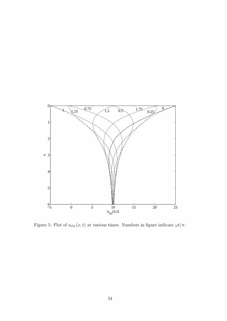


