
ECONOMIC GROWTH CENTER
YALE UNIVERSITY
P.O. Box 208269New Haven, Connecticut 06520-8269http://www.econ.yale.edu/~egcenter/
CENTER DISCUSSION PAPER NO. 814
SUPERVISION AND TRANSACTION COSTS:EVIDENCE FROM RICE FARMS IN BICOL, THE PHILIPPINES
Robert E. EvensonYale University
Ayal KimhiHebrew University
Sanjaya DeSilvaYale University
April 2000
Note: Center Discussion Papers are preliminary materials circulated to stimulate discussions and criticalcomments.

ABSTRACT
Labor markets in all economies are subject to transaction costs associated with recruiting,
monitoring and supervising workers. Rural labor markets in developing economies, where institutions such
as labor and contract law and formal employment assistance mechanisms are not in place, are regarded to
be particularly sensitive to transaction cost conditions. The inherent difficulty of measuring transaction
costs has limited studies on this topic.
In this paper, we analyze supervision activities reported in a cross-section survey of rice farmers
in the Bicol region of the Philippines. This survey is unique because it provides supervision data at the
farm task level. We present a simple optimization model in which supervision intensity increases the
productivity of hired workers, which is assumed to be lower than that of family members due to the
transaction costs. The model predicts that supervision intensity will increase with transaction costs. We
use different institutional conditions to proxy for transaction costs, and estimate the demand for supervision
time for four different classes of rice production tasks. The estimation strategy controls for selectivity in
both hiring and supervising. The results show a positive effect of transaction costs on supervision
intensity.
We then extend the analysis to a farm efficiency specification to test the proposition that
supervision activities improve farm efficiency. This framework allows us to relate institutional conditions
to farm efficiency directly and indirectly through their effect on supervision activities. We find that
transaction costs have a negative direct effect on farm efficiency, but this is partially offset by the positive
efficiency effects of increased supervision intensity. The results enable us to associate institutional
conditions with transaction costs and to draw policy inferences regarding the value of improved
institutional conditions.
KEYWORDS: Transaction Costs, Supervision, Labor Markets, Philippines
JEL CLASSIFICATIONS: 013, D23, J43, Q12

2
I. Introduction
Labor markets in all economies are subject to transaction costs associated with recruiting,
monitoring and supervising workers. Transaction costs in the labor market typically arise due to
information problems of two types: 1) moral hazard because the true work effort is not easily verifiable
and enforceable, and 2) adverse selection because information on the attributes of heterogeneous workers
is not readily available. Recruiting costs can also increase if communication and transportation networks
are weak so that the labor markets are segmented. Transaction costs will be lower in environments
where contract are easily enforced, information on workers and employers are readily available and labor
markets are well connected. The level of transaction costs affects labor and land contract choices and
family labor advantages. Rural labor markets in developing economies, where institutions such as labor
and contract law and formal employment assistance mechanisms are not in place, are regarded to be
particularly sensitive to transaction cost conditions. A number of studies of contract choice support this
contention. The inherent difficulty of measuring transaction costs, however, has limited studies on this
topic.
In this paper, we report an analysis of supervision activities based on a cross-section survey of
rice farmers in the Bicol region in the Philippines. This survey is unique because it provides supervision
data at the farm task level in addition to information on production activities and household characteristics
over a range of institutional conditions. It also provides barangay (village) level variables that help us to
quantify the institutional conditions. Our primary concern is to analyze the demand for supervision time on
survey farms. We develop estimates of the effect of different institutional conditions on supervision time
for four different types of rice production tasks.
We also extend the analysis to a farm efficiency specification to test the proposition that
supervision activities improve farm efficiency. This framework allows us to relate institutional conditions
to farm efficiency directly and indirectly through the effect on supervision activities. This enables us to

3
associate institutional conditions with transaction costs and to draw policy inferences regarding the value
of improved institutional conditions.
Only a few studies have formally studied the demand for supervision. Empirical studies are
especially rare because most farm level surveys have not explicitly measured supervision intensities.
Several studies have related the demand for supervision to wages and the size of work groups. Efficiency
wage models suggest that supervision may be substituted by wage premiums when monitoring is costly
(Bulow and Summers 1986). This justifies the finding of Groshen and Krueger (1990) and Kruse (1992)
that wages and supervision intensity are negatively correlated. However, if variations in shirking costs
among firms are more important than variations in monitoring costs, supervision and wages may be
positively correlated (Neal 1993). That is, if wages are high, the cost of shirking is higher for employers.
Supervision also depends on the size of the work group (Ewing and Payne 1999), but the sign of the effect
is ambiguous: scale economies in supervision make monitoring more cost-efficient in larger work groups;
on the other hand, large work groups are more difficult to supervise. To our knowledge, the literature has
not addressed the relationship between institutional conditions (or transaction costs) and supervision. We
hypothesize that the demand for supervision will be greater in high transaction cost environments.
In part II of this paper, we develop the specification utilized in this paper. In part III, we
summarize the data. Part IV reports our supervision demand estimates. Part V reports our farm
efficiency estimates. Part VI concludes with policy implications.
II. A Simple Model of Supervision Intensity
Assume that production is a function of effective labor (E) that is composed of family labor and
hired labor, according to the following specification:
E = Lf + [α + g(Ls/Lh + β Lf/Lh)] Lh (1)

4
where Lf is family labor, Lh is hired labor, and Ls is supervision (all in hours). Hence, family members
provide two separate types of labor: (1) conventional labor input; and (2) direct supervision of hired
workers. The effectiveness of hired labor is determined by the parameter α, the direct supervision
intensity (Ls/Lh) and the indirect supervision intensity (Lf/Lh). The parameter α represents the efficiency
of hired labor (relative to family labor) if there is no direct or indirect supervision. We assume that α is
between zero and one, implying that if only hired labor is employed, the effectiveness of a unit of hired
labor is lower than that of a unit of family labor if only family labor is employed. The most obvious reason
for this assumption is moral hazard. Indirect supervision refers to the fact that family members working
together with hired workers increases the effectiveness of the hired workers even if no direct supervision
is performed. The coefficient β, which is assumed to be between zero and one, determines the relative
effectiveness of indirect supervision intensity and direct supervision intensity. The latter is naturally
assumed to be more effective (β<1). If family members and hired workers are employed concurrently, the
parameter α has to be even smaller so that α+g()<1, otherwise if would be more efficient to use family
workers for direct supervision only.
Other than working on the farm or supervising hired workers, family members also have the
possibility to work off the farm. We allow the off-farm wage rate to be different from the wage paid to
hired workers. If family members and hired workers are similar in their earnings capacity then the off-
farm wage rate is expected to be lower than the wage paid to hired workers due to transaction costs. In
this case we will not expect family members to work off the farm. Family members will work off the farm
only if their earnings capacity is higher than that of hired workers.
The farm household is assumed to maximize income, which is the sum of farm income and off-
farm income:
I = f(E) + wn (L - Lf – Ls ) – wh Lh (2)

5
where I is income, f() is the production function, L is total time devoted to work activities by family
members (we assume that the labor-leisure choice is separable), wn is the off-farm wage and wh is the
wage paid to hired workers. Note that the price of farm output is normalized to 1.
Income maximization provides optimal values for hired labor, family labor, and direct supervision.
Any of these variables can of course be zero. Hired labor may be zero on small farms in which the returns
to family labor are higher than off-farm wages (Sadoulet et al. 1998). In this case there will also be no
direct supervision. Family labor may be zero on farms in which the returns to family labor are lower than
off-farm wages. Direct supervision may be zero on farms in which indirect supervision is almost as
efficient as direct supervision.
The alternative cost of a unit of time of family members is the same regardless whether it is used
for farm work or for direct supervision (it is the off-farm wage rate if family members work off the farm
or the marginal rate of substitution between consumption and leisure otherwise). Hence, the income
maximization problem is separable in the sense that family farm labor input and direct supervision can be
derived by maximizing effective labor input, given the (positive) values of hired labor input and total family
farm labor supply. The solutions to this maximization problem are:
Lf = (LT - δLh)/(1-β) (3)
Ls = (δLh - βLT)/(1-β)
where LT = Lf + Ls and δ = (g’)-1(1/(1-β)). It can be shown that Lf is positive if LT/(δLh)>1, while Ls is
positive if LT/(δLh)<1/β. Therefore, it is possible to have both Lf and Ls positive for reasonable values of β,
although the admissible range for this is declining as β approaches 1. However, given that both Lf and Ls
are positive, and plugging (3) into (2), income becomes linear in LT and Lh and hence income maximization
does not produce internal solutions for both LT and Lh. This means that having both Lf and Ls positive is

6
not compatible with income maximization. This result is supported by our data, which show that family
labor and direct supervision coexist in the same task in only about 3% of the cases.
Therefore, the decision on whether to work on the farm and indirectly supervise hired workers, or
to directly supervise only, is a discrete decision to be made by family members. Our focus in this paper is
on the direct supervision activities, hence we continue by looking at families who chose the direct
supervision path. For these families, plugging equation (1) in equation (2) and setting Lf to zero yields:
I = f{[α + g(Ls/Lh)]Lh} + wn (L – Ls ) – wh Lh (2)’
This can be maximized over Lh and Ls/Lh to get the optimal values of hired labor and supervision intensity,
respectively. The first order conditions are:
pf’(E) g’(Ls/Lh) - wn = 0 (4)
pf’(E)[α + g(Ls/Lh)] - wnLs/Lh - wh = 0
and the optimal supervision intensity can be derived from
α + g(l) = g’(l)( l + wh/wn) (5)
where l = Ls/Lh is the supervision intensity.
We cannot present closed-form solutions without specifying the g() function. However, we can
derive the signs of the effects of wages (wh and wn) and transaction costs (which affect α) on supervision

7
under the reasonable assumption that g() is a well behaved twice differentiable function with g’()>0 and
g’’()<0.
The supervision intensity, l, is a function of wh, wn and α. We obtain the first order conditions
with respect to each of these variables by implicitly differentiating equation (5).
For the hired wage, wh,
∂∂
lw
g l
g l w lww
hn
h
n
=− +
>' ( )
' ' ( ) [ ]0 (6)
The hired labor wage has a positive effect on supervision intensity. This is because an increase in
the hired wage increases the cost of shirking (lost wages) to the employer. In addition, a higher wage
increases the cost of hiring labor and reduces the amount of hired labor through a movement along the
demand curve. Effective labor can be partly restored by increasing the supervision intensity. This can be
achieved by reducing family supervision proportionately less than the reduction in hired labor, or even
increasing it. Here, we have ignored the efficiency wage argument where wages over and above the
reservation wage are given to reduce shirking by increasing the cost of shirking to the worker.
For the off-farm wage, wn,
∂∂
lw
g lw
w
g l lww
n
h
n
h
n
=+
<' ( )
( )
' ' ( ) [ ]
2
0 (7)

8
Supervision intensity will decrease with off-farm wages. The reasoning is quite straight-forward because
off-farm wages increase the opportunity cost of the farmer’s time.
For the shirking variable , α:
∂∂ α
l
g l lww
h
n
=+
<1
0' ' ( ) [ ]
(8)
This tells us that supervision intensity decreases when hired labor is more effective in the absence
of supervision. For example, if there is an effective incentive scheme (piece rate contracts, long-term
contracts, tenancy etc.) that acts as a self-enforcement mechanism for worker effort, the need for direct
supervision is less. We argue that the extent of shirking, or the magnitude of α, is a function of the
institutional conditions of the village. We expect the extent of shirking to be less in areas with well-
developed market institutions that provide alternative methods for work effort enforcement. Therefore,
weaker institutional conditions lead to a lower α and more supervision.
A Graphical Representation
The simplest treatment of supervision economics considers laborers to be subject to “shirking” or
lack of direction if unsupervised. Therefore supervision lowers hired labor costs by improving the
effectiveness of hired labor. In figure 1, we represent “shirking” costs as a negative function of
supervision intensity. In the previous section, we saw that the shirking costs increase when hired wages
(wh) increase, and when transaction costs are high due to institutional conditions (leading to a lower α) .
Therefore, we treat hired wages and transaction costs as shifters of the shirking cost function. In figure 1,
we illustrate four possibilities: (1) high wage, high transaction cost environment (curve A), (2) low wage,

9
high transaction cost environment (curve B), (3) high wage, low transaction cost environment (curve C),
and (4) low wage, low transaction cost environment (curve D).
We argue that transaction costs have a large effect on shirking costs. In low transaction cost
environments, labor markets are more complete, searching and recruiting costs are lower because of job
search programs etc., and legal institutions are in place to enforce efficient labor contracts.
The cost of providing supervision is the opportunity value of the farmer’s time. The time for
supervision must be diverted from off-farm work or from other farm tasks (including indirect supervision
by working with other hired workers). For low levels of supervision, this joint work-supervision activity
may be very low cost. The curve F represents the opportunity cost of supervision. If the farmer has an
elastic supply of time, the opportunity cost will be horizontal line at the off-farm wage. However, we
argue that most farmers are time constrained, as reflected by the very low levels of off-farm labor
participation (DeSilva 2000). In this case, the opportunity cost of supervision is the marginal rate of
substitution between consumption and leisure which is an increasing function of supervision intensity. In
fact, it is likely that the marginal cost of supervision (slope of curve F) would approach infinity, and there
will be a upper bound of supervision intensity at the labor time endowment level. The shift parameters
for curve F is the off-farm wage and the labor time endowment of the farmer (as reflected by family size
and demographic variables). The observed supervision intensity will be higher if the off-farm wage is
low, and if the farmer has a large endowment of family labor.
The farmer selects the optimal level of supervision (SA, SB, SC, SD) that minimizes the sum of
shirking and supervision costs (A+F, B+F, C+F, D+F). This provides net of supervision transaction costs
of TCA, TCB, TCC, TCD.
Three points merit attention here: 1) Given the low cost of joint work-supervision at low levels of
supervision, there is likely to be some minimum level of supervision (e.g. SD) below which supervision is
not reported as direct supervision by farm managers. We incorporate this in the empirical analysis by

10
estimating a selectivity equation where a probit on the choice to supervise is specified as a function hired
wages and transaction costs. 2) In our formulation, the chief determinant of supervision intensity is the
level of transaction costs, i.e. SA- SC > SC - SD and SB- SD > SA - SB. This claim is tested in the empirical
analysis by comparing the wage effects with transaction cost effects. 3) The observed (net of
supervision) transaction costs are represented by TCA, TCB, TCC and TCD. In figure 1, we see that,
conditional on wages, observed transaction costs are higher in high transaction cost environments.
However, the greater supervision intensity in high transaction cost areas would lead to a relatively larger
reduction in observed transaction costs in these areas. We estimate farm efficiency equations to isolate
these effects. We expect supervision intensity to have a positive effect on farm efficiency (by lowering
observed transaction costs), and high transaction costs to have a direct negative effect on efficiency (by
raising observed transaction costs). However, the assumption that high transaction cost environments
have larger observed transaction costs is based on the assumption that the supervision cost function is
fixed across environments. This may be unrealistic, because it is easy to visualize a remote village where
higher transaction costs are offset by lower supervision costs (due to lower off-farm wages, larger
endowments of family labor). In this case, we may find some cases where observed transaction costs
(and efficiency) are lower in remote high transaction costs environments.
Econometric Specifications
As a preliminary step in the empirical analysis of the determinants of supervision intensity, we
write the first-order approximation of the supervision intensity equation (the solution of equation 5) as
Ls/Lh = Xsδ + v (9)

11
where Xs is a vector of explanatory variables including wages, utility shifters and farm production
determinants, δ is a corresponding vector of coefficients, and v is a random approximation error.
Accordingly, we also specify the demand for hired labor as
Lh = Xhγ + u (10)
When one wants to choose a suitable empirical model to estimate the coefficients of (9), two selectivity
problems have to be addressed. First, some farms do not hire any outside labor and use family labor only.
Here supervision is not relevant. Second, some farms that do hire workers, decide not to supervise them.
Therefore, the sample of farms for which supervision intensity is positive is not a random sample, and
hence the supervision intensity equation (9) cannot be estimated by ordinary least squares.
We try three different approaches to correct for selectivity. The first approach is to use a binary
choice model for the hiring decision, and a censored regression model for the supervision intensity
equation, which comes into effect only if the first decision is to hire workers. The two models are
estimated jointly. Suppose now that we have a sample of farms that can be divided into three groups:
group A includes farms who do not hire labor, group B includes farms who hire labor but do not supervise,
and group C includes farms who hire labor and supervise. The likelihood function of this sample is:
∏ A pr(Lh ≤0) x ∏ B pr(Lh >0 and Ls/Lh ≤0) x
∏ C pr(Lh >0 and Ls/Lh >0)cd(Ls/Lh | Lh >0 and Ls/Lh >0) (11)
where ∏ A is the product over all the observations belonging to group A, pr() stands for probability and
cd(|) stands for conditional density. Assuming that u and v are jointly normally distributed with zero means,

12
standard deviations of σu and σv, respectively, and a correlation coefficient ρ, the likelihood function can
be written as:
∏ AΦ (- Xhγ/σu) x ∏ BΨ( Xhγ/σu , -Xsδ/σv , ρ) x
∏ C φ[(Ls/Lh -Xsδ)/σv (11)’
where φ and Φ are the probability density function and cumulative distribution function, respectively, of
the standard normal random variable, and Ψ is the cumulative distribution function of the standardized
bivariate normal random variables. The coefficients γ, δ, σv, and ρ can be estimated by maximizing (11)’.
One shortcoming of this approach, which is similar to the shortcoming of the familiar Tobit model,
is that the same coefficients and the same variables that determine the level of supervision intensity also
determine whether to supervise or not. For example, if there are fixed costs associated with labor
supervision, a variable that is related to these fixed costs will affect the decision to supervise but not how
much to supervise, given that supervision is positive. Our second approach allows for a separate equation
to determine whether to supervise. Specifically, this equation is formulated as:
M = Xmµ + ε (12)
and supervision is performed when M>0. Now, supervision intensity is observed only when Lh>0 and
M>0. We use a bivariate probit model with sample selection (Wynand and van Praag 1981) to model the
selection in two stages. The standard bivariate probit model is modified to incorporate the fact that the
supervision (M) exists only if hiring is positive. The likelihood function of this model is:
∏ A pr(Lh ≤0) x ∏ B pr(Lh >0 and M ≤0) x
∏ C pr(Lh >0 and M >0)cd(Ls/Lh | Lh >0 and M >0) (13)

13
Under the usual assumptions on the error terms, the likelihood function becomes
- ( X (- X
( A
'B
C
Φ Φ
Φ
β β β ρ
β β ρ
1 1 2 2 2 1 1
2 2 2 1 1
' '
' '
) , , )
, , )
x x x
x x
∏ ∏∏
−
(13)’
where Φ 2 is the bivariate normal distribution function and ρ is the correlation coefficient between the two
error terms. Jones (1992) applied this model to British data, and Garcia and Labeaga (1996) -to Spanish
data. Both could not reject the independence assumption.
In the third model we use, a standard multinomial logit specification is used for the selection
equation. The choice variable Y is defined as:
Y = 0 if Lh ≤0
1 if Lh >0 and M ≤0
2 if Lh >0 and M >0
and
Prob for and ( ) , ,'
'
Y je
ej
j i
k i
x
x
k
= =+
= =
=∑
β
β
β1
0 12 0
1
2 0 (14)
The sample used in the supervision equation is based on the choice Y=2.

14
A Model of Farm Efficiency1
The supervision demand model tells us that institutional conditions play an important role in
determining the intensity of supervision activities. In the second part of this paper, we estimate the direct
and indirect (through supervision) effect of institutional conditions on farm efficiency using a stochastic
production function approach (Aigner et. al 1977, Meeusen and van der Broeck 1977).
The production frontier, where Q is the output, and Z is a vector of observed inputs, such as land,
labor, fertilizer, seeds, machinery and draft animals is formulated as follows:
Q f Z u
where u U and U N
and N
i i i i
i i i u
i e
= −
=
( ; ) exp( )
~ ( , )
~ ( , )
β ε
σ
ε σ
0
0
2
2
(15)
We assume that the two error terms are distributed normal and half-normal respectively, and are
independent of each other. The two-sided error term captures the effects of unobserved stochastic
factors (e.g.weather shocks) and specification errors. The one-sided non-negative error term represents
“technical inefficiency” of the farmer or, more precisely, the ratio of the observed to maximum feasible
output, where maximum feasible output is determined by the stochastic production frontier (Lovell 1993).
Then, the technical efficiency (TEi) of farmer i can be expressed as,
TEQ
f Zui
i
ii= = −
[ ( ; ) exp( )]exp ( )
β ε (16)
1 This discussion in this section borrows heavily from DeSilva (2000)

15
It is straight-forward to estimate the stochastic frontier model using maximum likelihood methods.
Since our aim is to determine the effect of institutional conditions and supervision on farm efficiency, we
further define the one-sided error term, u, as follows:
u TE a F a B a S ei i i i i i= − = + + +log 1 2 3 (17)
where F is a vector of farm-level variables, B is a vector of institutional variables at the barangay level and
S is the level of supervision intensity. The error term ei is defined so that u is non-negative and half-
normally distributed.
The simplest way to estimate this efficiency equation is to regress the technical efficiency
estimates obtained from the stochastic frontier estimation on a set of explanatory variables (e.g. Pitt and
Lee 1981, Kalirajan 1981). However, such a two-step method is fundamentally incorrect because the
dependent variable in the OLS specification of equation (17) was assumed one-sided, non-positive and
identically distributed in the first step (Kumbhakar et. al 1991, Reifschneider and Stevenson 1991, Battese
and Coelli 1995). We adopt the more appropriate method of jointly estimating the frontier and efficiency
equations using maximum likelihood methods. We use the version of this method proposed in Battese and
Coelli (1995).
The coefficient a2 tells us the efficiency effect of the institutional environment, which can be
interpreted as a measure of transaction costs. If an explicit measure of supervision was not included, the
estimate of a2 will be biased because the demand for supervision is also a function of transaction costs as
argued in the previous section. In particular, we expect the estimate of a2 to be smaller in absolute value
when supervision is excluded because higher transaction costs may be partially compensated by
supervision. Although the inclusion of supervision gives us a better transaction cost measure, this may
cause endogeneity problems because both farm inefficiency and supervision intensity may be correlated

16
with the same unobserved variables (e.g. motivation, entrepreneurship). We correct for this by using the
predicted supervision from the demand equations as a proxy variable.
III. Data
The data used in this research are from the 1994 Bicol Multipurpose Survey, which was
conducted in Camarines Sur, the main province of the Bicol region of the Philippines. The sample consists
of 691 households from 59 different villages (barangays). The survey collected detailed information on
demographics, health, income, expenditures, and farm production. The most detailed information collected
was on the 264 households engaged in rice cultivation. Some of the households were cultivating rice on
more than one plot, and most of them had two crops per year. Hence, we have a total of 652 observations
on rice cultivation units by farm, plot, and season.
For each cultivation unit, labor input is reported for each of 16 work activities defined in Table 1.
The labor input is also reported separately for hired labor, family labor, and exchange labor. Exchange
labor is ignored because it occurs in less that one percent of the activities. In most activities, either hired
labor or family labor are reported. Hired labor and family labor are reported for the same work activity in
less than 3% of the cases. The cases in which hired labor is employed consist of slightly more than one
half of the cases, according to Table 1. However, there is considerable variation across work activities.
We have grouped work activities into four major types: land preparation, planting, caring, and harvesting.
Although there is still variation in the fraction of hired labor activities within the major types, much of the
variation seems to be between types. In harvesting activities, for example, hired labor consists of 85% of
the cases, while it is less than a third in caring activities. Table 1 also shows that almost two thirds of the
hired labor activities are supervised by family members. This fraction also varies across and within types
of activities. Also reported is the total amount of supervision time. From this we derive the supervision
intensity index Ls/Lh which is our dependent variable.
17
We estimate our models separately for the four different types of activities. We also tried to
estimate the models separately for each activity, but some of the samples were too small and many of the
results lacked statistical significance. As explanatory variables in the supervision intensity equation, we use
several groups of variables. The first group include hired labor wage and the off-farm wage, which come
straight out of our theoretical model. The second group consists of variables which determine the
effectiveness of supervision, reflecting the functional form of g() in our theoretical model. These include
the number of hired workers, a dummy indicator for hired workers that are employed under a time rate
contract, a dummy indicator for hired workers that were hired through a labor contractor, the land area of
the farm, a dummy for the rainy season, a dummy for plots which are located in the same barangay as the
residence of the farm operator, and two dummies for using gravity irrigation and pump irrigation (the
excluded group is rainfed plots). Also included in this group are a set of barangay-specific variables which
proxy for labor market conditions. These are the distance to the nearest city, a dummy for new road
construction in the last decade, and an urbanization index. The third group of explanatory variables are
household head characteristics and household demographic variables. These could affect the effectiveness
of supervision and also the amount of time devoted to work by family members (L). These variables are
the numbers of males and females in the household, and the sex, age and education of the head of
household. Table 2 includes definitions of the explanatory variables and their descriptive statistics.
IV. Supervision Demand Estimates
1. Land Preparation Activities
The first column in Table 3 reports the results of the tobit supervision model with selection. In the
selection equation, the barangay-level transaction cost variables show that there is more hiring in areas
with new roads and those that are less urbanized. The presence of new roads lowers transportation costs
and helps the labor market to function better. However, the urbanization effect is counter-intuitive and

18
difficult to interpret. The results also show that the probability of hiring-in labor is positively affected by
the farm size, age and education of the farmer, number of female adults in the household and the
presence of pump and gravity irrigation. The first four effects suggest that laborers are hired when the
household has a large land to labor endowment ratio. Education of the farmer appears to reflect the
opportunity cost of cultivation. The positive irrigation effects indicate that irrigated land is more intensively
cultivated, and requires more labor.
The tobit supervision equation is estimated for all households that hire-in labor. The farms that do
not supervise are treated as zero-censored observations. The transaction cost variables reveal that
supervision intensity is higher in barangays with higher transaction costs. Specifically, farmers in
barangays that are further from cities and those without new roads supervise more intensively. In addition,
the supervision intensity increases with the number of hired workers, and decreases with farm size. The
first effect supports the idea that large work groups are more difficult to supervise. The second effect
shows that opportunity costs of supervising increase as when the hired workers are spatially dispersed.
We also find that male farmers supervise more intensively.
The second column reports the results of the linear supervision model with a bivariate probit
selection rule. The bivariate probit selection rule first estimates the hiring-in choice and then, conditional
on hiring-in, estimates the choice to supervise. The coefficient estimates of the hiring-in equation is very
similar to the probit selection equation in Model 1. Conditional on hiring-in, we see that the number of
workers and the gender of farmer has a positive effect on the choice to supervise. The work group size
effect is interesting because it suggests the existence of some fixed costs that makes direct supervision
inefficient when there are only a few hired workers.
The linear supervision equation is estimated only for farmers that supervise. The selectivity
correction term is significant at the 10% level. Here again, we see a substantial positive effect of
transaction costs (distance to city and new roads) on supervision intensity. We also find that older and

19
more educated farmers supervise less intensively. This may be because they are more efficient at
supervising, or because their opportunity costs are larger. Unlike in the tobit supervision equation, the
worker and gender effects are not significant in the second stage equation. By estimating the choice to
supervise and the extent of supervision separately, we are thus able to separate out the fixed and variable
costs of supervision.
The third column reports the linear supervision equation with a selectivity correction based on a
multinomial logit selection rule. The results are reported for two choices, hiring without supervision and
hiring with supervision, relative to not hiring. Barangays with new roads are more likely to hire-in
workers with and without supervision. Similarly, age and education of the farmer and the presence of
irrigation increases the likelihood of hiring in both cases. Less urbanized barangays are more likely to
hire-in with supervision relative to both of the other choices. In addition, households with larger farms,
less male (and more female) adults, and a female head are more likely to hire-in without supervision.
These results suggest that households with high land to labor endowment ratios (as reflected by the farm
size and demographic variables) are likely to hire-in but do not have sufficient family labor to directly
supervise.
The selectivity term in the supervision equation is once again significant at the 10% level. The
rest of the coefficient estimates are qualitatively similar to that of Model 2. In particular, the transaction
costs have a positive effect on supervision intensity.
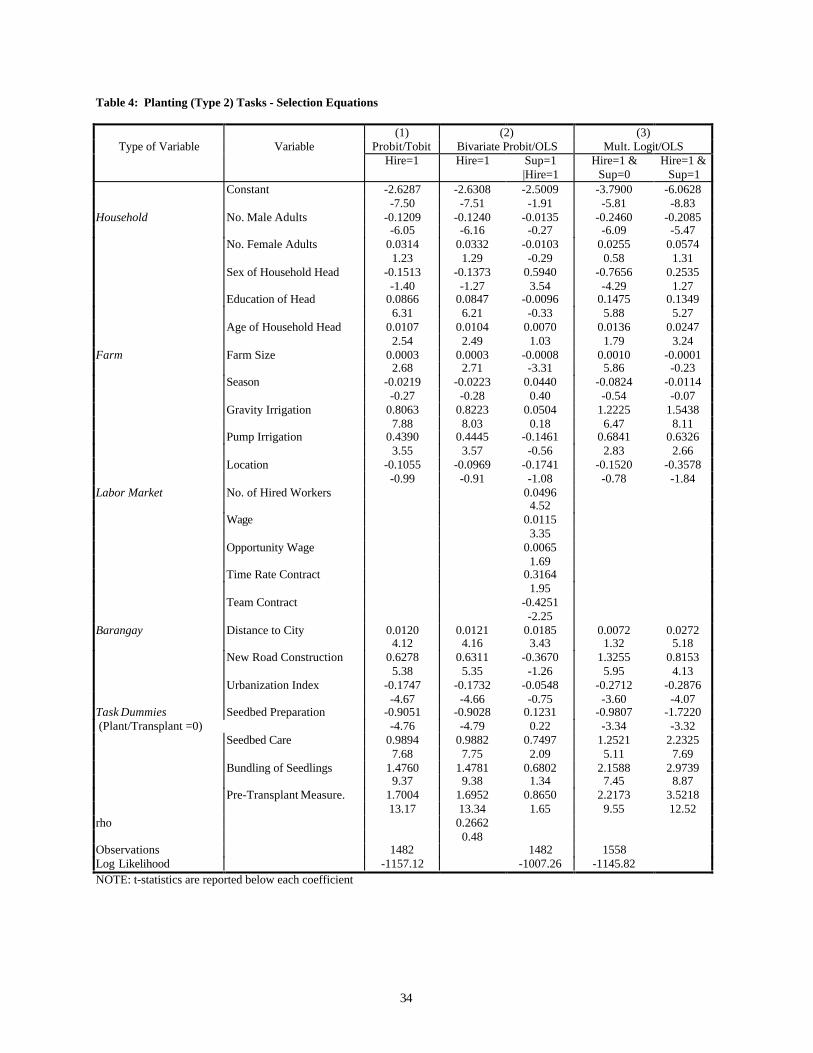
2. Planting Tasks
The first column in Table 4 reports the results of the tobit supervision model with selection for
planting tasks. In the selection equation, the barangay-level transaction cost variables have significant
effects on the choice to hire-in. Households in the more urban barangays and in those with new roads
participate more in the hired labor market. Conditional on these two variables, the probability of hiring-in

20
increases with distance to city. The farm size, age, education, irrigation and household composition
variables have similar effects to that of land preparation tasks.
In the tobit supervision equation, only the new roads variable has a significant expected sign
among the transaction cost variables. The supervision intensity also increases with the number of hired
workers and decreases with farm size. We also find that the type of labor contract has an important
effect on the extent of supervision. For example, workers that are hired on a time-rate basis are
supervised more because the time-rate contracts do not provide a self-enforcement mechanism for the
work effort of laborers. Workers that are hired as teams are supervised less intensively possibly because
of scale economies associated with teams, or alternative supervision methods (by team leaders etc.).
The second column reports the results of the linear supervision model with a bivariate probit
selection rule. Once again, the coefficient estimates of the hiring-in equation is very similar to the probit
selection equation in Model 1. Like the land preparation tasks, both the number of workers and the
gender of farmer have a positive effect on the choice to supervise conditional on hiring-in. For planting
tasks, the distance to city, wage and time-rate contracts also have positive effect on the choice to
supervise. The farm size and teams have negative effects. These coefficients have the expected signs.
The wage effect is especially interesting, and supports the conclusion of the theoretical model that the
reduction in hired labor due to high wages can be partially offset by increasing the supervision intensity.
The selectivity term is not significant in the supervision equation. The transaction cost variables
have the expected signs, although only the urbanization effect is significant. We also find a positive
education effect and negative gender and team effects.
The third column reports the linear supervision equation with a multinomial logit selection rule.
Barangays that are more urbanized and have new roads are more likely to hire-in workers with and
without supervision. The barangays that are distant from cities are more likely to hire workers with
supervision. Age, education and irrigation increase the likelihood of hiring in both cases. The number of

21
male adults in the household decrease the likelihood of hiring. However, the farm size and gender of
household head appear to affect only the decision to hire-in without supervision.
The selectivity term in the supervision equation is significant at the 5% level. Among the
barangay variables, urbanization and new roads have the expected signs and are significant. The distance
to city is insignificant. The wage effects are also negligible. However, we find that supervision intensity
increases if the household has male adults, if the farmer is resident in the same village as the farm and if
the farm size is large. The first two effects are intuitive and indicate the availability of family labor to
supervise. The third effect is the opposite of what we saw for land preparation, and is difficult to
interpret.
3. Caring Tasks
The first column in Table 5 reports the results of the tobit supervision model with selection for
caring tasks. The estimates of the selection equation are qualitatively similar to the estimates for planting
tasks. At the barangay level, distance to city, new roads, and urbanization increase the probability of
hiring-in. At the household level, the farm size, number of female adults, age, education, resident status
and irrigation have significant positive effects. The number of male adults has a negative effect.
In the tobit supervision equation, supervision intensity is high in barangays that are distant to cities.
However, the new roads variables has the wrong sign in this case. The supervision intensity also
increases with age, education and irrigation. The number of male adults is significant, but also has an
unexpected sign. The wage and contract variables are insignficant. The somewhat unexpected results
may be caused by the fact that the tobit equation confounds the choice to supervise with the intensity of
supervision.
The bivariate probit selection equation failed to converge under several different algorithms and
convergence criteria. This may be due to the small percentage (15%) of household engage in both hiring

22
and supervision for these tasks. The second column reports the linear supervision equation with a
multinomial logit selection rule. The results are similar to what we saw for planting tasks. Distance to
city is positive but not significant, while new roads are positive and significant. Unlike for planting, less
urban barangays have lower probability of hiring only when there is no supervision. Among the household
level variables, age, education and irrigation have a significant positive effect on hiring. The demographic
variables also have the expected signs. Farm size and the resident status have positive effects only in the
case of hiring without supervision.
The selectivity term is not significant in the supervision equation. In fact, only farm size and the
number of male adults have a significant effect on supervision intensity. The high standard errors in these
estimates reveal potential specification problems, or the inappropriateness of the supervision model itself in
the case of caring tasks. The weak results, and the convergence problems in Model 3, may both be
caused by the fact that caring is largely undertaken by family members and supervision in the form that is
observed in planting, harvesting and plowing, does not exist for these tasks.
4. Harvesting Tasks
The first column in Table 6 reports the results of the tobit supervision model with selection for
planting tasks. In the selection equation, the barangay variables are not significant. Education and
irrigation have significant positive effects on hiring. We also find a strong seasonal effect in hiring for
harvesting.
In the tobit supervision equation, distance to city and new roads have the expected signs but only
the latter is significant at 10% level. The supervision intensity also increases with irrigation, and decreases
with time rate contracts and education. The contract effect is the opposite of what the standard principal-
agent model suggests.

23
The second column reports the results of the linear supervision model with a bivariate probit
selection rule. The first stage probit equation is similar to the selection equation in Model 1, but gives
stronger estimates. The choice to supervise, conditional on the choice to hire, is negatively affected by
new roads and education and positively affected by wage, number of female adults and the gender (male)
of farmer. As in the case of planting, the wage effect confirms our theoretical result that supervision is
positively related wages.
The selectivity term is not significant in the supervision equation. The distance to city and new
roads have the expected signs, but only the former is significant at 10% level. However, we find a strong
negative effect for the number of workers indicating scale economies in supervision, and a strong negative
effect for time rate contracts. The negative time rate effect is peculiar to the harvesting tasks.
The third column reports the linear supervision equation with a multinomial logit selection rule.
The barangay effects are weak in the selection equation, except for a strong negative effect for new
roads in hiring with supervision. Seasonal effects are again more pronounced than for the other types of
tasks. In addition, irrigation and the number of female adults increase the probability of hiring with
supervision, and while education, area and gender (female) of the head increases the probability of hiring
without supervision.
The selectivity term in the supervision equation is significant at the 5% level. Among the
barangay variables, distance to city and new roads have the expected signs. This adds to the evidence
that supervision intensity is generally higher in environments with high transaction costs. We also find a
strong negative area, age and season effects, and the usual positive irrigation effects. The wage is once
again insignificant in determining the supervision intensity. The results seem to indicate that the wage
effect, if they exist at all, are captured in the choice to supervise and not in the intensity of supervision.

24
V. The Efficiency Estimations
Table 7 reports the results of the joint estimation of a stochastic production frontier and its
associated efficiency equation. The usual inputs (land, labor, fertilizer etc.) are included in the production
function. The equation for the one-sided efficiency error term is specified with two sets of variables: The
first includes farmer level variables such as age, education, ownership status, resident status and
supervision intensity. The second includes barangay-level variables such as distance to city, urbanization,
population and construction of new roads. The latter variables are included to capture transaction costs at
the market-level. The main purpose of this exercise is to determine whether intensive supervision
increases farm efficiency. Because barangay level transaction costs are likely to be highly correlated with
supervision intensity, we estimate the model with and without the barangay variables so that the direct and
indirect (through supervision) effects of transaction costs on efficiency can be identified. Because
supervision intensity may be an endogenous variable, we also estimate the model using the predicted
values from the supervision equation in Model 1 as a proxy for supervision intensity.
The first column reports results with the actual supervision intensities. The second column re-
estimates with predicted supervision values. For each case, we report the estimates with and without the
barangay variables. The production function estimates are very similar in all four cases. All inputs except
farm animals have a positive sign, although irrigation is not significant. Land and labor elasticities are the
largest as expected. A puzzling result is the substantial decreasing returns to scale (about 0.75) in the
production function. This may indicate that the simple Cobb-Douglas form is not appropriate in this case.
The negative estimates for farm animals is also likely to arise from the constant elasticity of substitution
assumptions because farm animals can be thought of as an inferior substitute (in some cases) to tractors.
In the efficiency equation, we find the expected efficiency effect of supervision. When the actual
supervision intensity is used and the barangay variables are omitted, the efficiency effects are large (8.24)
and significant at 10% level. When barangay variables are included, the magnitude of the effect drops by

25
about one-half (4.36) because the barangay variables independently have efficiency effects. When the
predicted supervision intensity is used, the efficiency effects are still positive but much smaller and less
significant. Here again, the inclusion of barangay variables reduces the magnitude of the effect. In
addition the supervision effects, we find that farmers who are male, more educated, older and resident in
the same village are more efficient. Owner-farmers, on the other hand, appear to be less efficient than
tenants. This may reflect a selection bias, because more enterprising farmers may have obtained
leasehold lands under land reforms.
Among the barangay variables, lower transaction costs appear to increase efficiency.
Specifically, we find that farms in more populated and urbanized barangays and those with new roads are
more efficient. The only surprising result is the positive efficiency effect of the distance to city. This tells
us that conditional on urbanization, population and other included variables, the barangays that are farther
from cities are more efficient. This may be a result peculiar to this sample that arises due to the
correlation between favorable climate and soil conditions with the distance to cities. The direct inclusion
of soil and climate variables would help to resolve this ambiguity.
VI. Conclusions
Direct supervision of hired workers is a directly unproductive activity that diverts a farmer’s
valuable time from other income generating activities. A farmer would engage in direct supervision only if
the effort of workers cannot be enforced adequately by self-enforcement mechanisms such as contracts.
The primary objective of this paper was to establish whether farmers respond to a weak institutional
environment (where there is little scope for formal contracting) by increasing the direct supervision of
workers. Our unique data set from the Bicol regions allows us to explicitly estimate supervision demand
equations. We measure transaction costs with barangay (village) level indicators of urbanization and
access to markets. Our results confirm that barangay-level transaction costs increase the intensity of

26
supervision for all types of farm tasks. Improving labor and contract laws and the access to markets will
reduce the need for direct supervision and enable farmers to intensify their own labor inputs in the farm or
work in off-farm activities.
We also test the hypothesis that supervision activity increases farm efficiency. This is done by
estimating production frontiers with both transaction costs and supervision intensity as determinants of
farm efficiency. As expected, we find that transaction costs decrease efficiency, but this effect is
partially offset by the positive supervision effect. This further supports our initial claim that direct
supervision is a reaction to a weak institutional environment.
The efficiency estimates can also be used to construct a barangay (village) level index of
transaction costs. We interpret transaction costs as the component of observed farm efficiency explained
by barangay level institutional variables. Because we include a measure of supervision intensity in the
efficiency estimates, the index represents the transaction costs net of supervision. In future work, we
plan to use this measure to test for transaction cost effects in a variety of farm and household decision
making issues. This will help expand the empirical literature on transaction costs which has so far been
limited to a handful of studies (Lanzona and Evenson 1997).

27
References
Aigner, D.J., Lovell, C.A.K. and Schmidt, P. “Formulation and Estimation of Stochastic FrontierProduction Function Models”, Journal of Econometrics, 1977, 6, 21-37.
Battese, G.E. and Coelli, T.J., “A Model for Technical Inefficiency Effects in a Stochastic FrontierProduction Function for Panel Data”, Empirical Economics, 1995, 20: 325-332.
Bulow, Jeremy I., and Lawrence H. Summers. “A Theory of Dual Labor Markets with Application toIndustrial Policy, Discrimination, and Keynesian Unemployment.” Journal of Labor Economics 4, July1986, 376-414.
DeSilva, Sanjaya (2000), “Land Leasing as a Substitute for Imperfect Labor Markets: Theory andEvidence from Sri Lanka”. Ph.D. Dissertation, Yale University, New Haven.
Ewing, Bradley T., and James E. Payne. “The Trade-Off Between Supervision and Wages: evidence ofefficiency wages from the NLSY.” Southern Economic Journal 66, October 1999, 424-32.
Frisvold, George B. “Does Supervision Matter? Some Hypothesis Tests Using Indian Farm-Level Data.”Journal of Development Economics 43, April 1994, 217-38.
Groshen, Erica L., and Alan B. Krueger. “The Structure of Supervision and Pay in Hospitals.” Industrialand Labor Relations Review 43, February 1990, 134S-146S.
Kalirajan, K. “An Econometric Analysis of Yield Variability in Paddy Production,”Canadian Journal of Agricultural Economics, 1981, 29: 283-294.
Kevane, Michael. “Agrarian Structure and Agricultural Practice: Typology and Application to WesternSudan.” American Journal of Agricultural Economics 78, February 1996, 236-45.
Kruse, Douglas. “Supervision, Working Conditions, and the Employer Size-wage Effect.” IndustrialRelations 31, Spring 1991, 229-49.
Kumbhakar, S.C, S. Ghosh and T.J. McGuckin “A Generalized Production Frontier Approach forEstimating the Determinants of Inefficiency in U.S. Dairy Farms,” Journal of Business and EconomicStatistics, 1991, 9: 279-86.
Lanzona, L.A. and R.E. Evenson, “The Effects of Transaction Costs on Labor MarketParticipation and Earnings: Evidence from Rural Philippine Markets,” Center Discussion Paper No.790, Economic Growth Center, Yale University, October 1997
Lovell, C.A.K., “Production Frontiers and Productive Efficiency,” in Fried, H.O., Lovell,C.A.K. and Schmidt, S.S.(Eds), The Measurement of Productive Efficiency, Oxford University Press,New York, 1993, 68-119.
Meeusen, W. and van den Broeck, J., “Efficiency Estimation from Cobb-DouglasProduction Functions With Composed Error”, International Economic Review, 1977, 18, 435-444.
28
Neal, Derek. “Supervision and Wages Across Industries.” The Review of Economics and Statistics 75,August 1993, 409-17.
Pitt, M.M. and Lee, L.F., “Measurement and Sources of Technical Inefficiency in theIndonesian Weaving Industry”,Journal of Development Economics, 1981: 9,43-64.
Reifschneider, D. and Stevenson, R. “Systematic Departures from the Frontier: A Framework for theAnalysis of Firm Inefficiency”, International Economic Review, 1991, 32: 715-723.
Sadoulet, Elizabeth, Alain de-Janvry, and Catherine Benjamin. “Household Behavior with Imperfect LaborMarkets.” Industrial Relations 37, January 1998, 85-108.
Wynand, P. and B. van Praag, “The Demand for Deductibles in Private Health Insurance: A Probit Model with Sample Selection,” Journal of Econometrics, 1981, 17: 229-52

29
Figure 1: Graphical Representation of Supervision and Transaction Costs
Costs
Supervision/Hour of Labor
A
B
C
D
F
SASBSCSD
TC
TC
TC
TCD
A+F

30
Table 1. Number of cases, cases with hired workers, and the incidence of supervision
Type of activity Activity Number Cases with hired workers Cases with supervisionNumber Name Number Name of cases Number Fraction Number Fraction
1 Land Preparation 1 Tractor labor 562 455 0.81 314 0.692 Animal labor 485 286 0.59 196 0.693 Repair of dikes 644 285 0.44 147 0.52
subtotal 1691 1026 0.61 657 0.64
2 Planting 4 Seedbed preparation 352 74 0.21 26 0.355 Seedbed care 330 31 0.09 5 0.166 Bundling of seedlings 305 155 0.51 87 0.567 Pre-transplant
measurement156 106 0.68 56 0.53
8 Plant/transplant 665 420 0.63 275 0.65subtotal 1808 786 0.43 449 0.57
3 Caring 9 Weeding 483 227 0.47 131 0.5810 Fertilizing 566 145 0.26 79 0.5411 Chemical application 611 213 0.35 108 0.5115 Irrigation control 312 53 0.17 11 0.21
subtotal 1972 638 0.32 329 0.52
4 Harvesting 12 Harvesting 612 520 0.85 356 0.6813 Threshing 571 498 0.87 398 0.814 Harvesting/threshing 47 30 0.64 24 0.816 Pre-harvest activities 8 7 0.88 0 0
subtotal 1238 1055 0.85 778 0.74Total 6710 3505 0.52 2213 0.63

31
Table 2 : Descriptive Statistics
Name Mean Definition
Supervision Intensity 0.2316 Supervision intensity (number of direct supervision hoursdivided by hours of hired work.
HIRE 0.5477 Dummy for the existence of hired labor.Number of Workers 4.2873 Number of hired workers.aWage 76.335 Daily wage of hired workers (peso).aOpportunity Wage 52.254 Opportunity daily wage of family members (peso), derived
from off-farm labor earnings.Time Rate Contract (Dummy) 0.3383 Dummy for a time-rate labor contract.Team Contract (Dummy) 0.076 Dummy for hiring workers through a contractor.Farm Size 208.61 Land area of the farm (hectares/100).No. Male Adults 3.8158 Number of adult male household members.No. Female Adults 3.815 Number of adult female household members.Season 0.5337 Dummy for the rainy season.Sex of Household Head 0.7927 Dummy for a male head of household.Education of Household Head 6.8403 Years of schooling of the head of household.Age of Household Head 58.145 Age of household head.Gravity Irrigation (Dummy) 0.4068 Dummy for using gravity irrigation.Pump Irrigation (Dummy) 0.2271 Dummy for using pump irrigation.Location (Dummy) 0.7908 Dummy for plots that are located in the same barangay as
the residence of the household head.Distance to City 23.648 Distance of barangay to nearest city (km).New Road Construction (Dummy) 0.7246 Dummy for new road construction since 1983.Urbanization 2.3925 Urbanization index (5=lowest, 1-highest).
a. the mean is calculated using observations with hired workers only.

32
Table 3: Land Preparation (Type 1) Tasks: Selection Equations
(1) (2) (3)Type of Variable Variable Probit/Tobit Bivariate Probit/OLS Mult. Logit/OLS
Hire=1 Hire=1 Sup=1|Hire=1 Hire=1 &Sup=0
Hire=1 &Sup=1
Constant -1.2178 -1.2163 -0.8159 -2.0755 -2.7932-3.52 -3.53 -0.81 -3.35 -4.75
Household No. Male Adults -0.0365 -0.0384 0.0308 -0.1153 -0.0322-1.74 -1.84 1.04 -2.92 -0.92
No. Female Adults 0.0559 0.0577 -0.0347 0.1425 0.06822.21 2.27 -0.93 3.22 1.64
Sex of House. Head -0.1457 -0.1315 0.3534 -0.4960 -0.0193-1.39 -1.25 2.40 -2.61 -0.10
Education of Head 0.0862 0.0867 0.0300 0.1186 0.15616.81 6.85 1.01 4.91 6.84
Age of Head 0.0193 0.0191 0.0067 0.0266 0.03534.63 4.60 0.86 3.47 4.93
Farm Farm Size 0.0003 0.0003 -0.0002 0.0010 0.00032.66 2.54 -1.14 4.11 1.37
Season -0.0958 -0.0945 -0.1012 -0.1023 -0.2019-1.28 -1.27 -1.09 -0.69 -1.47
Gravity Irrigation 0.3623 0.3760 -0.2372 0.8242 0.45453.98 4.14 -1.19 4.72 2.79
Pump Irrigation 0.5511 0.5551 0.1415 0.8755 0.99555.14 5.18 0.60 4.13 5.25
Location 0.0343 0.0383 0.2278 -0.3831 0.14180.32 0.36 1.77 -1.98 0.74
Labor Market No. Hired Workers 0.13622.97
Wage 0.00141.42
Opportunity Wage -0.0026-0.91
Time Rate Contract 0.11450.89
Team Contract 0.05620.41
Barangay Distance to City -0.0025 -0.0027 -0.0018 -0.0030 -0.0065-1.02 -1.08 -0.50 -0.60 -1.40
Road Construction 0.2682 0.2515 -0.0421 0.4599 0.40832.72 2.59 -0.27 2.50 2.41
Urbanization Index 0.0685 0.0699 0.0374 0.0426 0.14902.04 2.09 0.82 0.67 2.60
Task Dummies Animal Labor -0.8541 -0.8532 -0.2089 -1.3657 -1.4946(Tractor Labor =0) -8.43 -8.46 -0.70 -6.58 -8.24
Repair of Dikes -1.2151 -1.2144 -0.7717 -1.5045 -2.3800-12.83 -12.82 -2.14 -7.93 -13.17
rho 0.35310.54
Observations 1382 1382 1434Log Likelihood -1555.049 -1270.295 -1338.377NOTE: t-statistics are reported below each coefficient

33
Table 3 (continued): Land Preparation (Type 1) Tasks - Supervision Demand Equations
(1) (2) (3)Type of Variable Variable Probit/Tobit Bivariate Probit/OLS Mult. Logit/OLS
Constant 0.0007 1.9192 1.69610.00 2.61 2.64
Household No. Male Adults 0.0231 0.0049 0.00051.40 0.45 0.04
No. Female Adults -0.0120 0.0062 0.0082-0.53 0.45 0.60
Sex of Household Head 0.2011 -0.0484 -0.01802.53 -0.57 -0.24
Education of House. Head -0.0071 -0.0436 -0.0395-0.31 -2.98 -2.97
Age of Household Head -0.0008 -0.0076 -0.0069-0.14 -1.93 -1.85
Farm Farm Size -0.0003 -0.0001 -0.0001-2.24 -1.18 -0.79
Season -0.0138 0.0791 0.0638-0.24 1.50 1.29
Gravity Irrigation -0.1436 0.0007 -0.0083-1.25 0.01 -0.14
Pump Irrigation -0.1218 -0.3292 -0.3074-0.74 -3.04 -2.99
Location 0.1559 0.0287 0.02571.75 0.36 0.32
Labor Market No. of Hired Workers 0.0571 -0.0216 0.00952.23 -0.90 0.66
Wage 0.0004 -0.0006 -0.00020.67 -1.24 -0.48
Opportunity Wage of Farmer -0.0006 0.0013 0.0007-0.32 0.84 0.46
Time Rate Contract 0.0293 -0.0715 -0.03510.37 -1.08 -0.56
Team Contract 0.1290 0.1149 0.13391.63 1.76 2.09
Barangay Distance to City 0.0055 0.0085 0.00872.71 4.87 4.94
New Road Construction -0.2086 -0.2813 -0.2800-2.29 -4.30 -4.25
Urbanization Index 0.0323 0.0076 0.00321.01 0.32 0.13
Task Dummies Animal Labor -0.0140 0.2376 0.1958(Tractor Labor =0) -0.06 1.71 1.59
Repair of Dikes -0.2621 0.4325 0.3420-0.81 1.55 1.43
Sigma (1) 0.696737.88
Rho (1) -0.0506 -0.6972 -0.5822Lambda (2) & (3) -0.07 -1.77 -1.71
Observations 833 531 531R-squared 0.17612 0.17547
NOTE: t-statistics are reported below each coefficient
34
Table 4: Planting (Type 2) Tasks - Selection Equations
(1) (2) (3)Type of Variable Variable Probit/Tobit Bivariate Probit/OLS Mult. Logit/OLS
Hire=1 Hire=1 Sup=1|Hire=1
Hire=1 &Sup=0
Hire=1 & Sup=1
Constant -2.6287 -2.6308 -2.5009 -3.7900 -6.0628-7.50 -7.51 -1.91 -5.81 -8.83
Household No. Male Adults -0.1209 -0.1240 -0.0135 -0.2460 -0.2085-6.05 -6.16 -0.27 -6.09 -5.47
No. Female Adults 0.0314 0.0332 -0.0103 0.0255 0.05741.23 1.29 -0.29 0.58 1.31
Sex of Household Head -0.1513 -0.1373 0.5940 -0.7656 0.2535-1.40 -1.27 3.54 -4.29 1.27
Education of Head 0.0866 0.0847 -0.0096 0.1475 0.13496.31 6.21 -0.33 5.88 5.27
Age of Household Head 0.0107 0.0104 0.0070 0.0136 0.02472.54 2.49 1.03 1.79 3.24
Farm Farm Size 0.0003 0.0003 -0.0008 0.0010 -0.00012.68 2.71 -3.31 5.86 -0.23
Season -0.0219 -0.0223 0.0440 -0.0824 -0.0114-0.27 -0.28 0.40 -0.54 -0.07
Gravity Irrigation 0.8063 0.8223 0.0504 1.2225 1.54387.88 8.03 0.18 6.47 8.11
Pump Irrigation 0.4390 0.4445 -0.1461 0.6841 0.63263.55 3.57 -0.56 2.83 2.66
Location -0.1055 -0.0969 -0.1741 -0.1520 -0.3578-0.99 -0.91 -1.08 -0.78 -1.84
Labor Market No. of Hired Workers 0.04964.52
Wage 0.01153.35
Opportunity Wage 0.00651.69
Time Rate Contract 0.31641.95
Team Contract -0.4251-2.25
Barangay Distance to City 0.0120 0.0121 0.0185 0.0072 0.02724.12 4.16 3.43 1.32 5.18
New Road Construction 0.6278 0.6311 -0.3670 1.3255 0.81535.38 5.35 -1.26 5.95 4.13
Urbanization Index -0.1747 -0.1732 -0.0548 -0.2712 -0.2876-4.67 -4.66 -0.75 -3.60 -4.07
Task Dummies Seedbed Preparation -0.9051 -0.9028 0.1231 -0.9807 -1.7220 (Plant/Transplant =0) -4.76 -4.79 0.22 -3.34 -3.32
Seedbed Care 0.9894 0.9882 0.7497 1.2521 2.23257.68 7.75 2.09 5.11 7.69
Bundling of Seedlings 1.4760 1.4781 0.6802 2.1588 2.97399.37 9.38 1.34 7.45 8.87
Pre-Transplant Measure. 1.7004 1.6952 0.8650 2.2173 3.521813.17 13.34 1.65 9.55 12.52
rho 0.26620.48
Observations 1482 1482 1558Log Likelihood -1157.12 -1007.26 -1145.82NOTE: t-statistics are reported below each coefficient

35
Table 4 (continued): Planting (Type 2) Tasks - Supervision Demand Equations
(1) (2) (3)Type of Variable Variable Probit/Tobit Bivariate Probit/OLS Mult. Logit/OLS
Constant 0.0092 0.8064 2.04771.55 1.64 3.66
Household No. Male Adults 0.0217 0.0150 0.03020.92 1.42 2.91
No. Female Adults -0.0145 -0.0022 -0.0091-0.89 -0.22 -0.86
Sex of Household Head 0.1541 -0.2165 -0.34142.24 -3.72 -4.94
Education of House. Head -0.0091 0.0121 0.0060-0.62 1.89 0.89
Age of Household Head 0.0034 0.0015 -0.00151.09 0.72 -0.67
Farm Farm Size -0.0004 0.0001 0.0002-3.66 0.74 1.98
Season 0.0260 0.0079 0.00240.51 0.23 0.07
Gravity Irrigation -0.0836 -0.0694 -0.2534-0.58 -1.03 -2.82
Pump Irrigation -0.1055 0.0035 -0.0561-0.94 0.06 -0.92
Location -0.0301 0.0513 0.0941-0.43 1.15 1.97
Labor Market No. of Hired Workers 0.0074 -0.0066 -0.00522.63 -1.81 -1.55
Wage 0.0027 -0.0008 -0.00071.75 -1.09 -0.95
Opportunity Wage of Farmer 0.0023 -0.0008 -0.00061.52 -0.75 -0.67
Time Rate Contract 0.1349 -0.0230 -0.01401.89 -0.47 -0.31
Team Contract -0.2588 -0.1977 -0.2047-2.68 -2.89 -3.31
Barangay Distance to City -0.4225 0.0032 -0.0013-0.57 1.54 -0.56
New Road Construction -0.2476 -0.0621 -0.1057-1.92 -1.15 -1.94
Urbanization Index 0.0243 0.0448 0.07790.61 2.05 3.48
Task Dummies Seedbed Preparation -0.1612 -0.6025 -0.4150 (Plant/Transplant =0) -0.47 -3.42 -2.69
Seedbed Care 0.1736 -0.1789 -0.49390.83 -1.35 -3.27
Bundling of Seedlings 0.1279 -0.1254 -0.49160.45 -0.81 -2.80
Pre-Transplant Measurement 0.1323 -0.2017 -0.67050.43 -1.17 -3.12
Sigma (1) 0.569014.85
Rho (1) -0.1638 -0.0238 -0.4735Lambda (2) & (3) -0.32 -0.16 -2.51Observations 614 367 367R-squared 0.26201 0.27399NOTE: t-statistics are reported below each coefficient

36
Table 5: Caring (Type 3) Tasks - Selection Equations
(1) (3)Type of Variable Variable Probit/Tobit Mult. Logit/OLS
Hire=1 Hire=1 & Sup=0 Hire=1& Sup=1
Constant -3.8465 -3.2563 -10.8859
-10.77 -5.25 12.54Household No. Male Adults -0.0658 -0.1268 -0.1407
-3.43 -3.45 -3.71No. Female Adults 0.0952 0.1119 0.0739
4.63 2.84 1.73Sex of Household Head -0.0598 -0.3124 0.1889
-0.63 -1.90 0.94Education of House. Head 0.0796 0.0767 0.1703
6.39 3.64 7.33Age of Household Head 0.0189 0.0138 0.0600
4.64 2.00 7.78Farm Farm Size 0.0002 0.0005 -0.0003
2.07 2.68 -0.85Season -0.0364 -0.0681 -0.0570
-0.51 -0.50 -0.37
Gravity Irrigation 0.3675 0.6225 0.65913.88 3.75 3.41
Pump Irrigation 0.4669 0.4593 1.35844.00 2.30 5.98
Location 0.2273 0.4425 0.21622.15 2.45 1.06
Barangay Distance to City 0.0063 0.0072 0.00812.34 1.46 1.64
New Road Construction 0.4712 0.5138 1.12004.64 2.92 5.40
Urbanization Index -0.1191 -0.4602 0.0979-3.39 -6.60 1.43
Task Dummies Fertilizing 1.3951 1.2054 3.7765 (Weeding =0) 10.52 5.36 7.81
Chemical Application 0.6295 0.1612 2.1887
4.55 0.72 4.50Irrigation Control 0.9870 0.7479 2.8259
7.46 3.51 5.89Observations 1655 1735
Log Likelihood -1269.37 -1256.77
NOTE: t-statistics are reported below each coefficient

37
Table 5 (continued): Caring (Type 3) Tasks - Supervision Demand Equations
(1) (3)Type of Variable Variable Probit/Tobit Mult. Logit/OLS
Constant -6.8841 5.4131-8.78 1.09
Household No. Male Adults -0.0535 0.1020-1.95 2.12
No. Female Adults 0.0485 0.01911.51 0.53
Sex of Household Head 0.1735 -0.16261.08 -0.85
Education of House. Head 0.0741 -0.04964.22 -0.83
Age of Household Head 0.0267 -0.02214.17 -0.98
Farm Farm Size -0.0001 0.0013-0.46 4.72
Season -0.0098 0.0959-0.10 1.08
Gravity Irrigation 0.3251 -0.19772.24 -0.91
Pump Irrigation 0.6314 -0.66563.67 -1.30
Location 0.0629 -0.01690.39 -0.13
Labor Market No. of Hired Workers -0.0071 0.0078-0.48 0.85
Wage 0.0023 -0.00150.63 -0.50
Opportunity Wage 0.0068 -0.00161.94 -0.59
Time Rate Contract -0.0662 -0.1803-0.37 -1.00
Team Contract 0.1464 -0.05560.91 -0.37
Barangay Distance to City 0.0157 0.00464.08 0.96
New Road Construction 0.5341 -0.32363.44 -0.76
Urbanization Index 0.0058 -0.17120.11 -1.86
Task Dummies Fertilizing 2.3736 -1.4952(Weeding =0) 6.91 -1.04
Chemical Application 1.6324 -0.55535.10 -0.59
Irrigation Control 1.9652 -0.86805.99 -0.78
Sigma (1) 1.279821.75
Rho (1) 0.9970 -1.0014Lambda (3) 100.95 -1.09Observations 478 254R-squared 0.23414

38
Table 6: Harvesting (Type 4) Tasks - Selection Equations
(1) (2) (3)Type of Variable Probit/Tobit Bivariate Probit/OLS Mult. Logit/OLS
Hire=1 Hire=1 Sup=1|Hire=1
Hire=1 &Sup=0
Hire=1 &Sup=1
Constant 0.9043 0.7880 0.9387 -0.9259 -0.16641.77 1.59 2.06 -0.87 -0.18
Household No. Male Adults -0.0094 -0.0156 -0.0205 0.0271 -0.0373-0.31 -0.53 -0.73 0.46 -0.70
No. Female Adults 0.0252 0.0650 0.0758 0.0628 0.15450.71 1.87 2.41 0.90 2.44
Sex of Household Head -0.4026 -0.2842 0.4412 -1.1864 -0.3693-2.33 -1.69 3.13 -3.42 -1.12
Education of Head 0.0500 0.0446 -0.0811 0.1199 0.04882.51 2.20 -5.97 3.42 1.49
Age of Household Head -0.0012 -0.0009 0.0009 0.0054 0.0008-0.17 -0.12 0.16 0.46 0.08
Farm Farm Size -0.0001 -0.0001 -0.0001 0.0004 -0.0001-0.34 -0.70 -0.25 1.53 -0.57
Season -0.2212 -0.2166 -0.0570 -0.2539 -0.4118-1.92 -1.93 -0.57 -1.09 -1.96
Gravity Irrigation 0.2460 0.2862 0.1194 0.2543 0.48641.81 2.14 0.98 0.97 2.05
Pump Irrigation 0.3875 0.4576 0.2084 0.4293 0.81542.19 2.66 1.41 1.20 2.52
Location 0.2269 0.2430 -0.0029 -0.0750 0.49221.50 1.64 -0.02 -0.26 1.86
Labor Market No. of Hired Workers -0.0127-1.41
Wage 0.00232.44
Opportunity Wage 0.00501.35
Time Rate Contract -0.2072-1.69
Team Contract -0.1409-0.95
Barangay Distance to City 0.0035 0.0056 0.0021 -0.0035 0.01160.97 1.61 0.48 -0.43 1.58
New Road Construction -0.2720 -0.3932 -0.3474 -0.3945 -0.8089-1.75 -2.67 -2.69 -1.22 -2.78
Urbanization Index -0.0193 -0.0054 -0.0038 0.0768 0.0381-0.34 -0.09 -0.09 0.76 0.42
Task Dummies Threshing 0.2566 0.2947 -0.4209 1.9714 1.4365(Harvesting =0) 2.12 2.58 -3.31 3.82 3.57
Harvesting/Threshing 1.0518 1.15412.05 2.94
rho -0.9796-0.07
Observations 972 972 1055Log Likelihood -1336.344 -731.7669 -860.781Note: t-statistics are reported below each coefficient.

39
Table 6 (continued): Harvesting (Type 4) Tasks - Supervision Demand Equations
(1) (2) (3)Type of Variable Variable Probit/Tobit Bivariate Probit/OLS Mult. Logit/OLS
Constant 0.8617 1.0683 -0.53412.22 2.32 -0.61
Household No. Male Adults -0.0120 -0.0087 -0.0279-0.50 -0.51 -1.33
No. Female Adults 0.0379 0.0314 0.05711.54 1.00 1.57
Sex of Household Head -0.0093 -0.0920 0.1115-0.08 -0.91 0.67
Education of House. Head -0.0240 -0.0194 -0.0233-1.75 -1.21 -1.50
Age of Household Head -0.0044 -0.0054 -0.0069-0.86 -1.67 -1.96
Farm Farm Size -0.0001 -0.0001 -0.0003-0.39 -0.66 -1.91
Season -0.1630 -0.1762 -0.2251-1.82 -2.28 -2.51
Gravity Irrigation 0.1660 0.1561 0.18331.63 1.45 1.64
Pump Irrigation 0.2882 0.2865 0.35852.19 2.10 2.24
Location 0.1051 0.1113 0.36570.90 1.06 2.04
Labor Market No. of Hired Workers -0.0178 -0.0192 -0.0116-2.12 -2.72 -1.69
Wage 0.0004 0.0001 -0.00020.64 0.32 -0.54
Opportunity Wage 0.0018 0.0012 -0.00040.67 0.53 -0.21
Time Rate Contract -0.2136 -0.2178 -0.1382-2.10 -2.30 -1.68
Team Contract -0.1068 -0.0538 -0.0185-1.04 -0.54 -0.20
Barangay Distance to City 0.0049 0.0049 0.01091.49 1.77 2.38
New Road Construction -0.2079 -0.1835 -0.2472-1.79 -1.28 -1.64
Urbanization Index -0.0223 -0.0328 -0.0349-0.56 -1.21 -1.18
Task Dummies Threshing -0.3997 -0.4460 0.2632 (Harvesting =0) -3.46 -4.94 1.25
Harvesting/Threshing 0.90043.19
Sigma (1) 0.969283.53
Rho (1) 0.8888 0.8586 1.6371lambda (2) & (3) 10.87 1.49 2.15Observations 852 661 661R-squared 0.12209 0.13133NOTE: t-statistics are reported below each coefficient

40
Table 7: Farm Technical Efficiency Estimates
Supervision Intensity Predicted Supervision IntensityWithout Barangay With Barangay Without Barangay With Barangay
(1) (2) (1) (2)coefficient t-ratio coefficient t-ratio coefficient t-ratio coefficient t-ratio
Production FrontierConstant -0.8980 -2.40 -0.8086 -2.17 -0.9277 -2.53 -0.8521 -2.29Land 0.1697 6.60 0.1653 6.11 0.1649 6.60 0.1690 6.13Labor 0.2859 6.36 0.2822 7.12 0.2829 6.40 0.2764 6.22Seeds 0.0586 5.14 0.0573 4.91 0.0604 5.35 0.0590 5.09Fertilizer 0.0376 2.71 0.0400 2.82 0.0385 2.97 0.0399 2.88Threshers 0.0443 3.42 0.0459 3.50 0.0472 3.66 0.0459 3.57Tractors 0.0390 3.26 0.0382 3.09 0.0411 3.48 0.0396 3.28Animals -0.0090 -1.14 -0.0132 -1.79 -0.0078 -0.97 -0.0109 -1.36Chemicals 0.0959 4.63 0.0922 4.48 0.1014 5.92 0.0989 4.74Irrigation - Upland 0.0131 0.07 -0.0764 -0.42 0.0250 0.13 -0.0441 -0.25Irrigation - Pump 0.0876 1.57 0.0568 0.91 0.0837 1.44 0.0507 0.89Irrigation - Gravity 0.0394 0.55 0.0292 0.39 0.0405 0.57 0.0358 0.51
Inefficiency equationConstant 1.8280 2.13 3.6178 3.08 1.3672 0.75 4.1902 2.53Sex of Household Head -1.7415 -1.87 -0.9652 -2.60 -2.1583 -1.51 -1.6780 -1.75Ownership Dummy 0.7605 1.27 0.2399 1.26 1.0132 1.60 0.4816 1.97Education of Head -0.4826 -1.90 -0.2226 -2.86 -0.6155 -1.52 -0.4519 -2.27Age of Household Head -0.0554 -2.03 -0.0316 -2.14 -0.0803 -1.06 -0.0610 -1.96Supervision Intensity -8.2415 -1.86 -4.3608 -2.37 -1.9154 -1.59 -1.3826 -1.87Location -0.9600 -2.03 -0.3785 -1.61 -1.6033 -1.55 -1.0521 -2.06Distance to City -0.0371 -2.53 -0.0428 -1.97Barangay Population -0.0004 -2.27 -0.0007 -1.73New Road Construction -0.5949 -2.02 -0.5481 -1.86Urbanization Index 0.2212 2.02 0.3517 2.32
sigma-squared 3.8252 1.85 1.7253 3.48 5.2152 1.62 3.3353 2.16gamma 0.9531 33.51 0.8908 21.24 0.9652 42.51 0.9421 32.18
log likelihood function -498.24 -495.26 -517.22 -511.51LR test for one-sided error 76.05 82.00 69.24 75.64number of restrictions 8 8 *number of cross-sections 318 318 331 330number of time periods 2 2 2 2total number of observations 564 564 577 576


