DI

SC

US

SI

ON

P

AP

ER

S

ER

IE

S

Forschungsinstitut zur Zukunft der ArbeitInstitute for the Study of Labor

Son Preference and Children’s Housework:The Case of India

IZA DP No. 6929

October 2012

Tin-chi LinAlícia Adserà

Son Preference and Children’s Housework:

The Case of India

Tin-chi Lin Princeton University

Alícia Adserà Princeton University

and IZA

Discussion Paper No. 6929 October 2012

IZA

P.O. Box 7240 53072 Bonn

Germany

Phone: +49-228-3894-0 Fax: +49-228-3894-180

E-mail: iza@iza.org

Any opinions expressed here are those of the author(s) and not those of IZA. Research published in this series may include views on policy, but the institute itself takes no institutional policy positions. The IZA research network is committed to the IZA Guiding Principles of Research Integrity. The Institute for the Study of Labor (IZA) in Bonn is a local and virtual international research center and a place of communication between science, politics and business. IZA is an independent nonprofit organization supported by Deutsche Post Foundation. The center is associated with the University of Bonn and offers a stimulating research environment through its international network, workshops and conferences, data service, project support, research visits and doctoral program. IZA engages in (i) original and internationally competitive research in all fields of labor economics, (ii) development of policy concepts, and (iii) dissemination of research results and concepts to the interested public. IZA Discussion Papers often represent preliminary work and are circulated to encourage discussion. Citation of such a paper should account for its provisional character. A revised version may be available directly from the author.

IZA Discussion Paper No. 6929 October 2012

ABSTRACT

Son Preference and Children’s Housework: The Case of India* Son preference in countries like India results in higher female infant mortality rates and differentially lower access to health care and education for girls than for boys. We use a nationally representative survey of Indian households (NFHS-3) to conduct the first study that analyzes whether son preference is associated with girls bearing a larger burden of housework than boys. Housework is a non-negligible part of child labor in which around 60% of children in our sample are engaged. The preference for male offspring is measured by a mother’s ideal proportion of sons among her offspring. We show that when the ideal proportion increases from 0 to 1, the gap in the time spent on weekly housework for an average girl compared to that of boy increases by 2.5 hours. We conduct several robustness analyses. First, we estimate the main model separately by caste, religion and family size. Second, we use a two-stage model to look at participation into housework (as well as other types of work) in addition to hours. Third, we use mother’s fertility intentions as an alternative measure of son preference. The analysis confirms that stated differences in male-preference translate in de facto differences in girl’s treatment. JEL Classification: J13, J22, O15, J16 Keywords: son preference, child labor, housework, India, National Family Health Survey Corresponding author: Alícia Adserà Princeton University Woodrow Wilson School 347 Wallace Hall Princeton, NJ 08544 USA E-mail: adsera@princeton.edu

* An earlier version of this paper was presented to the Population Association of America (Washington DC), the Demography seminar in Princeton University and the Association for the Study of Religion, Economics and Culture (Washington DC).

2

1. Introduction

Besides playing, learning and socializing with peers, children in less developed countries are frequently

involved in a variety of labor activities that are generally referred to as child labor. Some of these activities

are geared to the production of marketable outputs, such as working for pay in a factory or helping with

farming and selling produce in the market. Others involve the provision of services for family members

that are not for market exchange. In this paper we focus on the latter: the household chores children

undertake for their families. In particular this paper analyzes whether son preference is associated with

larger gender gaps in the hours of housework children undertake in Indian families. In many societies

sons are favored both for cultural or religious reasons and because of their potentially larger future

contribution to household income and parental support. As a result the literature has shown different ways

in which girls are discriminated and receive differentially low human capital investments in health or

education, among other things (Pande 2003; Lee 2004; Connelly and Zhang, 2003; Mishra, et al. 2004).

Little research has been done on the role gender preference in child labor (except for Koolwal 2007) and,

to our knowledge this is the first study that examines the ramification of son preference in children’s

housework. Understanding the role parental attitudes play in children’s time and gender disparities of time

allocation should be of great interest both for academic and policy reasons.

Housework is a non-negligible part of child labor in which around 60% of children in our sample are

engaged. In fact recent research has adopted a more generous definition of child labor to include

household chores (Kurosaki et al. 2006, Edmonds 2006, Basu et al. 2009). Helping with chores is an

integral part of children’s life in many parts of the world (Zelizer 1985; Montgomery 2009), perhaps the

most common form of labor provided by children. Pooling the Multiple Indicator Cluster Surveys (MICS)

data of the United Nations Children’s Fund (UNICEF) for over 30 developing and under-developed

countries, Edmonds (2008) shows that children aged 10-14 spend more time on household labor than in

market oriented work. Ignoring household labor would “frequently understate total hours worked by a child

by a factor slightly greater than 2” (Edmonds 2008, p.15). Edmonds (2008) shows that children who are

heavily involved in market work (e.g. > 12 hours per week) tend to perform a few additional hours of

domestic chores, but not vice versa. Despite its prevalence, housework has been an elusive area in the

3

study of child work since most of the previous studies focus exclusively on market-oriented activities (e.g.

wage employment) or production for the household’s own consumption (e.g. farm labor).

In this paper we use the National Family Health Survey of India, 2005-2006 (NFHS-3), a nationally

representative sample of Indian households to examine the relationship between son preference and the

level of children’s housework. India is a relevant case since child labor remains common (Basu, Das and

Dutta 2003, 2009) and a preference for sons still prevails with varying intensity across society (Das Gupta

et al. 2003; Chung and Das Gupta 2007, Bhat and Zavier 2003,Jayaraman, Mishra and Arnold, 2009,

Gaudin 2011). Worldwide, girls have traditionally performed more household tasks than boys, but in this

paper we hypothesize that this gap grows with son preference, as parents reduce boy’s burden of

household chores. We construct a measure of son preference based on mother’s ideal proportion of sons

(Clark 2000, Koolwal 2009, Lin 2009). To test our hypothesis, we use both OLS and random-effects

models of hours of housework for all children and run a set of robustness test to see how the results vary

across family size, religion, cast and specification of the SP variable. Son preference in all these models

is correlated with an increase in girls’ relative burden of housework of around 2.5 hours per week. Next,

we implement a two-stage model to take into account participation in housework and also on other types

of work, separately. Finally we use intended fertility as an alternative way to measure son preference in a

restricted sample of families that have one boy and one girl.

Section 2 presents the conceptual framework of our hypothesis. The description of the data and the

construction of the index are included in Section 3. Section 4 presents all the different analysis and

section 5 concludes with a brief discussion of the implications of results and possible extensions.

2. Conceptual Framework

In societies where boys are preferred over girls, the literature has shown ways in which girls are

discriminated, such as excess female infant mortality due to neglect and malnutrition (Das Gupta, 1987;

Kishor 1993, Rosenblum 2012) and differentially low human capital investments in health (Pande 2003)

or education, among other things (Lee 2004; Connelly and Zhang, 2003; Mishra, et al. 2004). No

research has been done on the role of gender preference in housework, the most prevalent form of child

4

labor. India is a relevant case to use for this analysis since both child labor (Basu, Das and Dutta 2003,

2009) and a son preference remain relatively common (Das Gupta et al. 2003, Bhat and Zavier

2003,Jayaraman, Mishra and Arnold, 2009,).

In many Indian households, it is customary that children help with farming, family business, or engage in

domestic chores (such as cooking, fetching water) for several reasons.1 First, over two-thirds of the

population still lives in rural areas and many lack sufficient infrastructure such as running water (IISP

2007, World Bank 2012). Families need to spend additional time to maintain the basic functioning of daily

life and children with appropriate physical strength become involved in many of these chores as they

grow up (such as washing clothes or fetching water). Second, the Indian workforce remains largely

agricultural, nearly 50% in 2009 (Ministry of Labor and Employment 2010). Agricultural production in

India is labor-intensive and dominated by small holders (Edmonds 2003, Birthal, Joshi, Roy, and Thorat

2007); thus, children become the natural helpers when farming requires more labor input. Third, despite

rapid economic growth since 2000, the distribution of income and wealth has remained highly unequal; a

large proportion of Indians still live below the country’s poverty line (World Bank 2012). Because of

poverty or near-poverty, children may need to engage in economic activities (helping with farming or

family business) to ensure family survival (Basu and Van 1998) and household appliances (e.g. washer,

stove) may not be affordable to many families that rely on manual labor instead.

The definition on what constitutes “children’s work” or “child labor” is not uniform in the literature. Earlier

literature (e.g. Basu and Van 1998) defined - “work” or “child labor” as activities that strictly resulted in

marketable outputs, such as wage employment or helping with family business. Lately research papers

have adopted a more liberal definition which also includes household chores (e.g. Kurosaki, Ito, Fuwa,

Kubo, and Sawada. 2006; Edmonds 2006; Basu, Das, and Dutta 2009). This broader definition seems to

be a better choice in assessing how children’s welfare is influenced by different types of activities. For

example, in assessing how labor influences schooling, there is no reason to define “work” as market work

exclusively, because children cannot study when they are engaged in housework even if does not

1 Wage employment, contrary to public perception, is relatively uncommon. Using a national sample in the year of 2000, Basu et al. (Basu et al. 2003) showed that less than 1 percent of sample children engaged in regular or casual wage work.

5

generate marketable outputs. Also, there is little evidence suggesting that one type of work is more

“benign” or “harmful” to children than other types of work. Last but not least, excluding housework as a

part of definition of child labor would grossly underestimate the burden on girls; worldwide, girls perform

more housework than boys (Edmonds 2008).

A number of microeconomic studies have examined factors associated with children’s work in South Asia,

including household wealth (Basu et al. 2009), siblings’ contribution/substitution (Edmonds 2006),

exogenous shocks such as trade reform (Edmonds and Pavcnik 2005), mothers’ education (Karusaki et

al. 2006) and mother’s labor force participation (Self 2011). Other research has investigated the extent to

which children’s work and schooling are substitutes, including Hazarika and Bedi (2006), or Karusaki et al.

(2006). Few studies have focused exclusively on housework as the outcome variable except for Webbink,

Smits, and de Jong (2011). Webbink et al. (2011) examined factors associated with housework performed

by children in 16 developing countries including India. They used the mean difference in age between a

husband and wife and the proportion of married women living with the husband’s original family to

indicate “traditionalism” and patriarchy of an area. Interestingly, the two contextual variables are

significantly associated with housework only among boys but not girls in Asia. We pursue this line of

analysis here. We focus, however, on the extent to which son preference mediates the intra-household

allocation of children chores in a distinct way than other measures of traditional gender arrangements is

the question.

In many societies sons are favored over daughters for a variety of social, economic and religious reasons

(Arnold, Choe, and Roy 1998; Das Gupta et al. 2003; Pande and Astone 2007). There are two primary

determinants of the differential treatment of men and women in these cultures. The first is related to

cultural or religious traditions (Arnold et al. 1998; Chakraborty and Kim 2010). Since many of these

societies are patrilineal, only men can continue the family lineage and daughters after married traditionally

move with their husband’s family. Also, men or sons play unique roles in many religions. For example,

according to Hindu tradition, sons are “needed for cremation of the deceased parents, because only sons

can light the funeral pyre” (Arnold et al. 1998: p301). Bhat and Zavier (2003) show how, in India, Hindus

and particularly Sikhs display the highest levels of son preference. Similarly, across castes, the behavior

6

of those that have achieved high ritual status (“Sanskritized”), usually conforms to male-preference with

regard to dowry, and marriage, among other things (Chakraborty and Kim 2010). Lately, families of lower

castes with high economic resources have also imitated those behaviors that reflect son-preference and

tried to marry up their daughters (hypergamy) (Agnihotri 2000, Gaudin 2011).

The second reason is related to the instrumental value of sons, or more broadly, to socio-economic

consequences of the male dominance in many areas of a society. Sons (or men) may have higher

earning potential and may be perceived as better providers of old-age support to parents than daughters

(or women). In agricultural societies, sons are an important source of labor for family farming. Labor

market opportunities for women remain more constrained worldwide than men’s in most countries

regardless of their development stage (Rosenzweig and Schultz 1982; Kishor 1993; Berik and Biglinsoy

2000; Bahttacharya 2005).

If parents are interested in eventually realizing (and, potentially, benefiting from) the value of a son, they

need to invest in their sons’ human capital. Doing housework contributes little to sons’ human capital

buildup. Thus, parents would rather have sons engaged in education, or other training activities (such as

acquiring skills from family businesses) that are expected to help to generate income for the family in the

future. An implication of this claim is that children with higher earning potential will be treated more

favorably and receive more family resources (Rosenzweig and Schultz 1982). This may take the form of

better quality of care, more time of play and leisure, and potentially less household chores. On the

assumption that excessive housework is unhealthy, parents will refrain from assigning much housework

to sons in order to maintain their health capital. Sons’ health is instrumental to higher earnings in the

future, and to better odds to assist parents as they age, and to continue the family lineage.

Accordingly in those societies that display son preference, a daughter is not expected to be the primary

source of old-age supports, regardless of prior parental investments. In patrilineal societies, a daughter is

expected to leave her biological family once she is married, and to typically assume the responsibility of

caring for the husband’s family (Das Gupta et al. 2003). The expected loss of daughters after marriage

further reduces the incentives of parents to engage daughters in education or in other long-term

investments. Helping with daily chores is a way parents to ask daughters to contribute to the family.

7

Of course a relatively higher burden of housework among girls may simply result from parents’ belief that

a girl should be good at housework skills in order to be socially fit once she enters adulthood. Those

gender role attitudes are closely related to both son preference and the division of housework, generally

viewed as a woman’s realm. Naturally, gender roles ideology also influences the demand for sons. If

parents strongly believe that the best role women can play is homemakers but not breadwinners, they

may prefer more sons to ensure old-age support. However, it is important to note that gender role

ideology is not a synonym for son preference: a mother may have no differential preference on the

gender of her offspring, while she still insists that girls should learn housekeeping to be socially fit.

Because of its strong linkage with son preference (Shu 2004) and gender division of housework (Coltrane

2000), in robustness analysis we explore the role of media exposure as a proxy for gender role

orientation. .

Finally it should be clear from the previous discussion that preference for sons does not result from “taste

of discrimination” against girls (Folbre 1984). An excessive amount of housework may be unhealthy for

both boys and girls, but there is no evidence suggesting that parents welcome daughters’ housework

burden on their time and heath while opposing housework assignments to sons. The preference for sons

does not result from parents benefiting from daughters’ disutility, but rather from their lower earning

potential or their secondary status in patrilineal family systems (Das Gupta et al. 2003);

As a result of all the different considerations of how parents perceive the instrumental values of sons

discussed in this section, we expect a greater gender difference in time spent on housework among

children in families that display strong son preference than in those where there is no such preference (or

where there even is a “daughter preference”).

3. Data and Variables

We use the National Family Health Survey of India, 2005-2006 (NFHS-3), a survey administered to a

nationally representative sample of Indian households and that follows the structure of the Demographic

and Health Surveys (DHS). NFHS-3 collected information from 109,041 households within over 3,000

primary sample units (PSU) -- villages in rural areas and census blocks in cities-- across all Indian states.

8

In each household, individual interviews were conducted among all men and women aged 15-49

regardless of their marital status. A total of 124,385 eligible women were interviewed and asked about

their fertility preferences, among other things. In addition to the basic demographic characteristics, more

extensive information was also provided for children aged 6-14 in the household. Given the structure of

the survey and our research questions, the units of analysis in this paper are children aged 6-14 who live

in the same household with their mothers. Our sample includes a total of 85,831 children, born to 46,070

eligible women. While mothers in our sample have only 1.9 children with complete interviews, on average

they have 3.3 children, because many of them fall outside the 6-14 age range.

The outcome variable is mother-reported hours of housework performed by her children during the survey

week, as recorded in the “Child Labor Module” of the survey. Housework refers to tasks that are

necessary to maintain the functioning of a family, but are not intended for market exchange nor involve

any payment for performance. In this study we use the terms “housework”, “household chores” or

“household labor” interchangeably. Examples of housework include cleaning, shopping, collecting

firewood, or caring for younger children. The original wording of the relevant questions in the survey is as

follows: 1) “During the past week, did (Name) help with household chores, such as shopping, collecting

firewood, cleaning, fetching water, or caring for children?” (If yes, go on to the next question). 2) “Since

last (Day of the week), about how many hours did he/she spend doing these chores?”

The module that the NFHS-3 adopted in this survey was synchronized with and is similar to that of

UNICEF’s Multiple Indicator Cluster Survey (UNICEF, 2011), widely used by researchers who study child

labor worldwide. Note that unpaid work in farm labor or helping with a family business does not count as

housework by UNICEF’s or in the Demographic Health Surveys (DHS). Consistent with general patterns

found by previous research (see Edmonds 2007 for a review); the majority of children’s labor input in

India took the form of domestic work, whereas less than 15% of Indian children were involved in market

work, including working for household or non-household members. In the distribution of hours of

housework during the survey week, there is a cluster of responses at zero hours, for around 50% of the

boys and close to 40% of the girls. To address this issue, in the empirical section we will study both the

intensive and the extensive margin of housework. Further to address the right-skewedness of the

9

distribution, we will use a lognormal model in the statistical analysis. Finally, the data exhibits evidence of

heaping, with a systematic pattern of clustering at multiples of seven, presumably because people tend to

report the hours of work per week by multiplying the hours per day by seven. This is not unusual in self-

reported hours of work and as long as there is no bias in clustering, the point estimators will remain

unbiased, although with a larger standard deviation. Results in the paper are robust to running the

analyses separately only for those clustering hours.

Son Preference: Our predictor variable of interest is the extent of son preference of the mother. In this

paper we measure it by the ideal proportion of sons calculated with the method employed in Clark (2000),

Koolwal (2009) and Lin (2009), among others. We use information from the following two separate

questions on fertility preferences included in the survey to construct it.

1. “If you could go back to the time you did not have any children, and you could choose exactly the

number of children to have in your whole life, what number would that be?”

2. “How many of these children would you like to be boys? How many would you like to be girls? For

how many would gender not matter?”

From these two questions we obtain three numbers: (1) the ideal number of sons, (2) the ideal number of

girls, and (3) the number of children whose gender would not matter to mothers. Then the ideal proportion

of sons is calculated as

For a woman desiring more sons than daughters this measure is greater than 0.5 and suggests a

preference for sons. For any child whose mother states that “sex doesn’t matter”, we assign an equal

weight of 0.5 to the number of desired sons and daughters. Thus, if a woman feels indifferent about the

sex of all her children, her “son preference index” (SP) is 0.5, regardless of her total desired number of

children. This method represents an improvement over simply calculating the share of sons on the ideal

family size by taking the number of sons wanted over the total number of children, as done in Bhat and

Zavier (2003). It allows for a larger dispersion of the measure of son preference and discriminates over

10

different family structures and preferences on the number of girls. In that regard, our index of son

preference has similar advantages as the SP measure employed by Gaudin (2011), namely, the

difference between ideal number of boys and ideal number of girls divided by the ideal family size. It is

worth noting that in the NFSH-3 survey a significant minority (13.7%) of the women explicitly states that

her children’s sex does not matter. In the distribution of the SP index there are large clusters at 0.5

(preference for balanced gender distribution) and 0.67 (when two-thirds of the children are sons) with,

respectively, 68% and 22% of the responses at those values in the weighted sample. Around 2.5% of the

respondents express some extent of girl preference (SP<0.5). For some of the analyses, we create a

dummy variable that equals one for those who express son preference (who account for 29.5% of the

sample) and pool together those who prefer more daughters (i.e. ideal proportion < 0.5) and those who

prefer a balanced composition (i.e. ideal proportion = 0.5) in the reference group.2

A natural concern with these measures as with any measure that uses subjective answers from

individuals is that the subjects may provide a socially desirable answer instead of their true preference

when inquired about their ideal sex composition for children. For example, a well-educated woman with

strong son preference may claim that she desires one boy and on girl, even if in fact she wants all her

children to be boys. This kind of bias is inherent to the question. However, it is difficult to measure what

types of women are more likely to misreport preferences (e.g. either mothers with high education or those

with low education). In addition these measures are exposed to the risk of ex-post rationalization when

women’s answers are affected by the current composition of their offspring. An extensive literature notes

that the concern of rationalization can be addressed by introducing appropriate controls in the models as

we do (Bhat and Zavier 2003, Pande and Astone 2007, Gaudin 2011). In section 4.4 we supplement the

main analysis that employs SP as defined here with another variable that indicates whether women who

already have two children desire additional children. This measure based on fertility intention is likely less

2 In robustness analyses not presented here we also use a three-level categorical variable that measures whether the ideal proportion of sons is greater than, equal to, or smaller than 0.5 (similar to that employed by Pande and Astone 2007) or alternatively, we run the analyses in a restricted sample that excludes women who express girl preference (and results are even stronger than in the full sample and significant). Estimates are available upon request.

11

subject to women’s intentional misreporting or ex post rationalization than the ideal proportion of sons

(Bankole and Westoff 1998).

Control Variables: Our models include a large set of control variables. First, we add several interaction

terms among children’s sex, place of residence, and age. We do so to control for the fact that there are

urban-rural and gender divides in hours spent on household chores and those gaps widen as children

grow older. In general, at any given age, girls in rural areas spend the most hours on housework, followed

by girls in urban areas, boys in rural areas, and finally boys in urban areas.

Further we use available information on whether a child has ever attended school in the previous year, as

well as the time in the survey week that a child spent on market-oriented work and farming for both family

members and non-family members separately. Although we expect these activities to be negatively

associated with the level of housework children undertake, the literature notes that it is unclear whether

these activities are real substitutes among themselves or whether, in many instances, they occur

simultaneously (Edmonds 2007). Wealth measures, the number of brothers and sisters and the number

of family members are also included in the questionnaire. We expect the need of housework to be

positively associated with the size of the family and negatively associated with improving material

conditions (Basu and Van 1998). We use the survey’s wealth index to represent household material

conditions, and rescale it by dividing it y 10,000. The wealth index, ranging from -18 to 24, is generated

directly by NFHS using factor analysis calculated over the full sample of households and its units have no

direct interpretation. We control for whether the family is Muslim, to take into account their traditionally

larger family sizes and lower son preference. Following original research by Dyson and Moore (1983) we

create a variable that embeds all families living in Punjab, Haryana, Uttar Pradesh (including Delhi),

Rajasthan, Gujarat and we label it North.3 Son preference is particularly strong in Northern India and we

are interested to see whether our findings prevail once we control for this regional difference (Miller 1981,

Arnold, Choe, and Roy 1998; Dyson and Moore 1983; Bhat and Zavier 2003). Finally, all models include

a set of state-level measures: GDP per capita, infant mortality and population density.

3 Results are robust to the use of a set of marginally different definitions of North or Northwest India (for example, including Himachal Pradesh, Jammu or Kashmir) found in the literature and in the Indian Census (Dyson and Moore 1983; Das Gupta et al. 2003; Chung and Das Gupta 2007, Bhat and Zavier 2003).

12

Descriptive analysis: The first rows of Table 1 present descriptive statistics of the variables included at the

family level, comprising fertility preferences of the mother, parents’ characteristics and other family

background characteristics. Regarding our main variable of interest, the mean desired proportion of sons,

0.56, indicates a moderate level of preference for sons over daughters: the average a woman wants

slightly more than half of her children to be male.

Most families (70.5%) live in rural areas, a third of them live in the North and the head of the household is

Muslim in only 14.8% of them. These figures are slightly higher but quite close to the national profiles in

2005 (IIPS 2007). The high share of rural families accounts for both the large number of individuals (6.3)

and large number of children (3.4) in the household. The average educational attainment of parents is not

high: 3.5 years of schooling for mothers and 6.0 years for fathers. Further, only between 35 and 40% of

the mothers are literate. The variation in all state-level characteristics is substantial.

In the second part of Table 1 we include variables regarding children’s characteristics, including age, sex,

school attendance and whether and how long they have participated in different types of work during the

survey week. Slightly more than half (51.8%) of these children are boys, and the average age of the

sample children is 10. Most (79.4%) of the children had some schooling in 2005, although the survey did

not inquire whether the children attended school regularly.

The majority (59.5%) of children helped their families with household chores during the survey week; less

than 7.2% worked for non-household members and less than 7.4% worked with household members on

activities such as farm labor, family business or street vending. The high prevalence of household labor

and the low frequency of market work—either working for household or non-household members—are

consistent with the pattern reported in other child labor research. Among those who helped their families

with housework, on average they provided 9.6 hours of household labor per week. For the entire sample,

the average hours spent on household chores is 5.7 hours. The average number of hours worked for non-

household members as well as for household member for all children is only 0.9 per week.

We start by examining a basic cross-tabulation between son preference and children’s housework labor

during the survey week. Consistent with our hypothesis, the gap in the time spent on housework between

13

a boy and a girl increases substantially with son preference. When the ideal proportion is zero, boys

actually do a bit more housework than girls. But as son preference increases, girls do increasingly more

housework. The difference between girls and boys in hours of housework grows to 2.66 on average

among those with SP between 0 and 0.5, and to 3.81 hours among those with SP over 0.5 (both

significant at the 0.001 level). In addition, total hours of housework performed (the work of boys and girls

combined) are larger as the measure of son preference increases. Since son preference is likely

endogenous, it is bound to be jointly determined with other household decisions. The observed increase

in hours of housework is likely associated with wealth and urban-rural differences in the demand for

housework. Families in rural areas tend to have worse material conditions and require more housework

labor for their daily activities than those in urban areas, both of which are associated with an increase in

overall hours of housework performed by children. Similarly, these families tend to report a stronger

preference for male offspring. We expect that some of the observed differences will be less pronounced

as we control for wealth and rural residence in the statistical analysis.

We suspect the manifestation of son preference is more explicit as children get older, since older children

can undertake more physically strenuous tasks. To explore this idea, the left hand side of Figure 1 plots

at each age the average hours of housework during the survey week, broken down by children’s sex and

level of son preference expressed by the mother (with either SP> 0.5 or SP<=0.5). Figure 1 shows that at

any given age, girls (the two solid lines) spend more time on housework than boys (the two dash lines).

Furthermore, the boy-girl difference, within-girl difference (between those in households with son

preference and the others), and within-boy difference (between those in households with son preference

and the rest) grow largely in proportion to age. Thus, a model that focuses on proportional change (such

as a log-normal model) may be appropriate to examine the relationship between son preference and

hours in housework. For both boys and girls, son preference is associated with more hours of housework,

but girls perform proportionally more additional hours than boys under son preference. This pattern is

consistent with the fact that the increase in housework among girls is substantially greater than boys’ as

the ideal proportion of sons grows from zero to one.

14

4. Empirical Analysis

4.1 Basic Models of hours of housework

To investigate the effect of parental son preference on children’s housework, we start with basic OLS

estimates of the following model.

Yhij = b0· Girlhij + b1· SPhi + b2· (SPhi x Girlhij) + ∑CXhij+ uhij ,

where Yhij represents hours of housework performed by child j in family i in PSU h, ,SP is our index of son

preference, Girl refers to the gender of the child, X is a vector of control variables and uhij the error term.

Our hypothesis states that the gap between the hours a girl spends on housework over boys’ grows with

son preference. The change in the difference between hours of work of girls over boys is captured by the

interaction term, b2. In the models presented in this section we use both specifications of son preference

described in section 3: either a continuous scale or an indicator for whether the desired proportion of sons

is strictly greater than 0.5.

Table 2, columns (1) to (4), displays OLS estimates of hours of housework undertaken by children aged

6-14 using a continuous index of SP. The model in column (1) includes only the three basic. Coefficients

indicate that SP is associated with more hours of housework and that girl’s in families with a higher index

of SP also undertake a relatively higher load than boys; around 4.2 hours more per week for families with

a SP equal to one compared to those with SP equal to zero. Column (2) includes a set of interactions

among the gender, age and place of residence of the child. In the following column an additional set of

covariates controls for the child’s school attendance and hours employed in other forms of work as well

as family composition, religion, wealth and parental education. Column (4) presents the most complete

specification that also encompasses state characteristics and controls for North India and its interaction

with the gender of the child. As more covariates are added into the model, the coefficient for the

interaction between SP and girl decreases somewhat in size but remains highly significant at 0.1%.

Consistent with the hypothesis, results in column (4) indicate that after all the child, family and geographic

15

controls are included, the gap in time devoted to housework between girls and boys is 2.65 hours larger

in families with high son preference than in those with strong daughter preference.

In column (5) we estimate the most complete specification in column (4) with a random-effects regression

(xtmixed procedure in Stata 11), as frequently done by labor economists when analyzing hours of work

(e.g. Lundberg and Rose 2001), to study how sensitive our results are to alternative methods. We

consider a three-level hierarchy formulation, including children, family and primary sampling unit (PSU)

and redefine the error term in our model as follows uhij =ph+ ahi + ehij , where ph are the random effects at

the PSU level, ahi are random effects at the family level, and ehij the error term. Measurements within the

same family may be correlated because of shared family environments, and measurements within the

same PSU may be correlated due to common social customs. The random-effects model, however,

assumes multivariate normality (Teachman et al. 2001), a condition rarely met in most empirical data. It

also imposes the strong assumption that the family and PSU specific effects are uncorrelated with the

other covariates in the model. Still, the significant coefficient of 2.52 for the interaction of SP and girls in

column (5) is in line with OLS results. In column (1) of Table 3 we run the same random effects model

with the binary definition of son preference. The estimated coefficient implies that son preference (SP>

0.5) is associated with a 0.86 hour increase in the gender gap. The magnitudes of random-effects are

appreciable in both models, indicating a high level of between-family and between-PSU heterogeneity (or

within-family and within-PSU correlation). Further, these findings are robust to alternative methods,

including negative binomial regression and zero-inflated negative binomial regression (available from

authors).

To better visualize the implied association between son preference and housework, we predict the hours

of housework for each child based on the random-effects model in column (5) of Table 2, with covariates

set at their observed values and random-effects at zero. Then we aggregate the hours of housework by

children’s sex and level of son preference. Figure 2 clearly shows that son preference is associated with a

relative greater burden of housework for girls. It also indicates another interesting pattern: total hours of

housework, for boys’ and girls’ combined, increase with the level of son preference, although the gap is

not as pronounced as in the simple cross-tabulation comparison where household material conditions or

16

rural residence are not controlled for. Furthermore, the change in the difference in the time spent on

housework comes largely from girls’ increasing housework input. As Figure 2 illustrates, when the ideal

proportion for sons grows from 0 to 1, the time an average girl spends on housework increases by 1.7

hours (from 5.4 to 7.1), but the hours for boys decrease only by 0.8 hours (from 4.4 to 3.55). One post-

hoc explanation for the additional hours among girls is that families with a preference for sons adhere

more to traditional gender roles, tend to live more in rural areas and consider essential for females to be

skillful in housework. Thus, to train their daughters to be “socially fit”, parents in these families tend to

involve girls in additional household responsibilities, regardless of household material conditions.

Predictions using estimates of column (1) in Table 3 produce the same pattern: boys in families with son

preference (SP>0.5) work 0.15 fewer weekly hours of in the house than those living in families with no

son preference, whereas girls work around 0.7 more hours.

With regard to the additional covariates, results underscore the importance of jointly considering

children’s age, sex and whether they live in rural or urban areas. Consistent with descriptive statistics,

older children perform more housework; the coefficient for children’s age is around 0.5 and highly

significant (p< 0.001). The coefficient for girl is negative, primarily because of the large and significant

interaction coefficients of girl both with age, around 0.49, and with rural residence, around 0.25, as well as

the coefficient for the three-way interaction among age, sex, and rural areas, around 0.15 (all at p <

0.001). Similarly, the main effect of rural areas becomes negative once child and family characteristics

are included. Taken together, these interactions suggest that the burden of housework is the greatest

among girls in rural areas and that both the urban-rural and gender gap in housework grows with

children’s age.

Overall the estimated coefficients for family characteristics are slightly smaller in the random effects

models than in OLS and fall within expectations. Children perform less household chores in families with

better material conditions, if they have attended school in 2005, or if they have a better educated mother.

To address the concern that school attendance is potentially jointly determined with hours of work and

that this may affect our estimate, in column (2) of Table 3 we exclude this variable from the model and

show that our coefficient of interest remains stable. A mother’s indifference about children’s gender is not

17

significantly connected with more housework of children, but desiring more than four children is correlated

with 0.40 more hours of housework. The number of siblings is positively associated with hours of work in

OLS estimates, but the number of sisters is insignificant in the random effect regressions. In robustness

analysis we include instead either the number of younger brothers and older sisters of each child or the

number of children aged 0 to 5 in the household. Research shows that the presence of an elder sister is

associated with a lower level of housework and the reverse is true when a child has a younger brother (or

younger siblings) (Emerson and Souza 2007). The literature suggests the burden is particularly high for

the eldest sister, who spends extra-time looking after younger sibling or supplementing family income

(Parish and Willis 1993). In robustness analyses not presented here, we find that having one elder sister

is associated with 0.54 fewer hours of housework, but having one younger brother with 0.55 more hours

(both at p< 0.001). In column (3) of Table 3 the number of young children aged 0 to 5 in the household

significantly correlates with increases in the amount of housework for children in our sample.

Consistent with Edmonds’ analysis (Edmonds, 2007), it is unclear whether different types of labor

activities are substitutes for each other. Working one additional hour for non-family members is

associated with only 0.01 fewer hours of housework , but working one additional hour for family members

on market production is associated with 0.17 more hours of household labor in the random effects models.

Finally, children in Muslim families, both boys and girls, perform less housework than their counterparts in

non-Muslim families (most of which are Hindu). Conversely, children in North India, where severe son

preference has been documented (Miller 1981, Arnold, Choe, and Roy 1998; Dyson and Moore 1983;

Bhat and Zavier 2003) undertake more household tasks than those in other areas. Boys in the North

undertake 0.87 more hours of housework than boys in other regions, and the parallel figure for girls is

1.57 (= 0.87+ 0.7, p< 0.001). Finally, children in states with higher population density and infant mortality

rates devote more hours to housework whereas those in relatively richer states do less.

4.2 Robustness

In the last columns of Table 3 we explore more in depth some nuanced relationships between son

preference, housework and other children characteristics.

18

Age: To better understand the role of age, in column (4) of Table 3 we insert both an interaction between

the child’s age and maternal son preference and a three way interaction of those covariates with the

gender of the child. As expected the estimated coefficient for the three-way interaction is highly significant

and implies an opening of the gap between girls and boys living in families with strong son preference as

compared to those with girl preference of 0.68 hours of work per year they age. We obtain similar results

in a specification with the binary SP index (not presented here), and produce the predictions of total hours

of housework by son preference (ideal proportion of sons > 0.5 or <= 0.5) and children’s sex displayed in

the right hand side of Figure 1. The projected pattern fits nicely the observed data (the left panel), except

for some underestimations among girls aged 12-14. Parental sex preference exerts little influence on

boy’s provision of housework, but such a preference is clearly associated with higher levels of girls’

involvement in household labor that increase in relative terms as they age.

Caste: Another important dimension that has been shown to explain variation in son preference as well as

sex ratios is caste (Arnold et al. 1998, Chakraborty and Kim 2010, Gaudin 2011). We define a high-cast

variable that includes individuals who do not belong to a scheduled caste, scheduled tribe, or other

backward class. Caste is missing in 9% of the observations in the survey. The reference category of this

variable includes both low-caste and no-caste families (such as Muslim or Christian). High-caste families

in our sample do not have a significantly higher level of son preference than the rest. Not surprisingly in

high-caste families children do less housework than in the other families and the gender gap is slightly

smaller. Average hours of housework in high-caste families are 5.96 for girls and 3.62 for boys, a 2.3

hours difference, whereas in the others, the average for girls is 7.51 compared to 4.42 for boys, a 3.1

hours difference.

In column (5) of table 3 we introduce in the model a control for whether children live in a high-caste

household , interactions of this variable with either son preference or girl as well as a three-way

interaction of all of them. Even if they are positive, the coefficients for the two-way interactions of high

cast with girl and with son preference are not significant. Only the three-way interaction is highly

significant and negative with a value of -2.64. The main coefficient for SP*Girl increases with respect to its

original value in column (5) of Table 2 from 2.5 to 3.04 indicating that on average the gender gap is

19

slightly larger in the sample of non-high-cast families when we separate them. In net terms, however, son

preference is still associated with a positive gender gap in high-caste families, though much smaller in

relation to the average number of hours girls perform than for other families.

Religion: Previous literature has highlighted important religious differences in the intensity of the parental

preference for male offspring. In general results suggest that Hindus and, particularly, Sikhs (mostly

concentrated in Northern India) have stronger son preference than Christians and Muslims (Bhat and

Zavier 2003; Gaudin 2010). As a result we hypothesize that the relevance of maternal son preference is

likely to be less associated with actual differences in household behavior among the large minority of

Indian Muslim than among other groups. In columns (6) and (7) of Table 3 we run the most complete

specification separately for the sample of Muslims and non-Muslims. Findings confirm that in the sample

of Non-Muslim children the estimated coefficient for the interaction of SP and the gender of the child is

highly significant and larger than in previous estimates. Conversely, son preference is not associated with

an increase in the gender gap of housework among Muslim children.

Family size: Next we analyze whether the association between son preference and the gender gap in

housework varies by number of children in the family. There are several reasons for conducting this

analysis. First, the relationship between fertility outcomes and fertility preferences is dynamic.

Preferences predict outcomes; but outcome themselves (i.e. the birth of a daughter or a son) impact the

way many mothers rationalize them, particularly if they do not accord to their initially stated preferences.

Unfortunately we lack longitudinal data to examine this dynamic process. However, by breaking down the

sample by parity, we hope to obtain a snapshot of the extent/level of son preference at different levels of

fertility.

Second, a separate analysis by family size reduces the complexity of controlling for sibling structure. The

total number of children and their sex composition by rank may influence how parents allocate household

duties, as shown in Tables 2 and 3. In the full sample, however, it is difficult to control for the precise

sibling structure since we observe 736 unique sex combinations of children across families. When we

20

restrict the analysis to families of either two or three children the number of possible sex compositions

across families drops to either 4 or 8 respectively.4

A caveat to conducting the analysis separately by family size is the sample selection bias introduced by

not partitioning the sample randomly. Breaking down the current sample by family size is certainly not a

random partition, as family size depends on factors such as parents’ age and fecundity. Furthermore, the

number and sex composition of children is endogenous since families trying to have a boy may stop once

they achieve it (Clark 2000, Arnold et al. 2002). In that regard a large family size may indicate a family’s

search for sons and larger families are more likely to have more daughters. A recent paper by Rosenblum

(2012) uses the sex of the first child as an instrument of family size to look at the implications of these

stopping rules on the health and mortality of boys and girls. Moreover a relatively smaller variation in son

preference expected among larger families may bias the estimates of the impact of son preference on

differential housework assignment downwards. Of course the presence of sex selective abortion, another

means to achieve a desired number of boys, reduces both the share of girls in the family and the overall

household size (Das Gupta 1987, Das Gupta et al. 2003, Arnold et al 1998, 2002, Bhat and Zavier 2003).

Basic cross-tabulations indicate that larger families are overrepresented in rural areas where the need for

children’s input in the household is greater and the conventional gender division of work more prevalent.

Only around 60% of families with two children in our sample live in rural areas, whereas the same

proportion is 73% for those with four children. Similarly, the average ideal proportion of sons (SP index)

increases with the number of children, from 0.53 in families with two children to 0.56 in families with four,

whereas the share for whom the children’s gender does not matter moves down from 22% to 9%.

Table 4 presents OLS estimates for one-child families, and a linear model with random-effects for families

with more than one child. For ease of comparison, column (1) includes the results for the entire sample

presented earlier in column (1) of Table 3. The interaction between girl and the binary index of son

preference (SP>0.5) is significant for all family sizes, though only at 5% in the sample of single-child

4 The appendix presents the complete combinations of covariates included in the models for each family size to account for the sibling structure in the family (the gender and the order of each child as well as the structure of the remaining children). In families with more than one child, the reference group is the last-born son in an all-boy family; in one-child families, the reference group is a boy.

21

families. The magnitude of the coefficient decreases with family size. Single girls in families with son

preference undertake around 1.6 hours more of work than boys in similar families. The gender gap in

families with son preference moves down from 1.1 hours in those with two children, 0.73 hours in those

with three children and to only 0.6 in those with four children. The decrease in size is possibly related to

the fact that family size is endogenous to son preference, and to the larger availability of siblings to share

the housework.

Results from the sibling structure suggest that older children (in terms or their rank in their family)

undertake more household tasks than younger ones. Consistent with the estimate from the full sample,

the presence of a sister is in general associated with fewer hours of housework in families of three and

four children. The older-sister disadvantage is particularly strong in families of four children that are more

likely to reside in rural areas. Detailed results are available online.

Media Exposure

As noted in the conceptual section, gender role attitudes may mediate the relationship between the

preference for sons and gender differentials in children’s housework. Egalitarian gender roles are often

emphasized in mass media, and watching TV exposes people to new ways of thinking, and leads to

attitudinal change (Bhat and Zavier 2003; Barber and Axinn 2004; Chung and Das Gupta 2007). Jensen

and Oster (2009) find that the introduction of cable TV in selected rural areas closes a great chunk of the

difference in son preference in those villages compared to urban areas. Since the NFHS-3 does not

explicitly inquire parents about gender role orientation; we use mother’s exposure to media (TV, radio and

newspaper) as a proxy.5 Over 20% of the families report having no access to any of the three types of

modern media. Mothers’ low media exposure is closely associated with a larger gender gap in housework

as well as with girls spending more hours on housework. When we introduce this covariate in the models,

both alone and interacted with girl, the coefficient for SP*Girl decreases somewhat in size (around 15-

20%), but remains highly significant. We recognize that media exposure is likely an endogenous variable

5 Media exposure is measured as the sum of the score of frequencies of access to TV, radio and newspapers. For access less than once a week, we assign a frequency 0.5; for at least once a week, we assign a frequency 3 and for almost daily access, the frequency assigned is 7. Thus the variable ranges from 0 (no access) to 21. The overall mean score is just 5.8.

22

correlated with son exposure -which likely accounts for this finding. Because of its exogenous nature,

Jensen and Oster (2009) are able to use the timing of the introduction of cable TV in a panel of Indian

villages as an instrument for the increased autonomy of women. Unfortunately the available regional

detail and sample size in NFHS-3 precludes us from using a similar type of instrument and we choose to

omit this covariate from the main tables in the paper. However, results are available upon request.

4.3 A Two Part Model of Children’s Work

As mentioned in the descriptive analysis, 40% of the eligible children did not contribute any housework

during the survey week and only 7.2% and 7.4% worked for non-household members and household

members, respectively, on alternative activities such as farm labor, family business or street vending.

Although the validity of the findings of the paper does not depend on the level of children participation in

these activities, the high frequency of zero hours of work in the sample cannot be ignored. To better

investigate the relevance of son preference on both the extensive as well as the intensive margin of child

labor and whether it is correlated in a distinct way across different types of labor, we estimate a set of

models of participation (whether the child does any work at all or not), hours of work for the whole sample

and hours of work among those who exert positive effort in one activity. Each column in Table 5 presents

the coefficient for the interaction of SP and girl for the three types of labor and for different estimation

methods. In the first row, the gender gap in children’s participation in some form of work among families

with son preference is only significant in the logistic models of housework. The second row of Table 5

shows that in the sample of all children, the gender gap in hours of housework is positive, but the gap for

market-related work (both with household and non-household members) is negative and marginally

significant at 10%. This is consistent with the hypothesis presented in the conceptual framework that

families with strong son preference choose to devote boys’ time to more productive activities (preferably

to build their human capital). When the sample is limited to children with positive hours in an activity, the

gender gap is positive and significant in all models of housework and negative (but not significant) for

other types of work.

23

To better illustrate how participation matters, we employ a two-part model (Pohlmeier and Ulrich 1995) to

produce the predictions for an average boy or girl at different levels of son preference in Table 6.6 First,

we estimate whether a child provides household labor or not using a random-effects logistic model .Then,

among those who help with household chores, we estimate how many hours they spend on it using a log-

normal model with random-effects. We assume the random effects in the first stage are independent from

those in the second stage.7 The estimated interaction between son preference and girl is positive and

significant at 1% level in both stages (see the appendix). Predictions in the first row of table 6 show how

son preference (SP > 0.5) is associated with a large gender difference in the probability of providing

household labor during the survey week. When the ideal proportion of sons is less than or equal to 0.5,

there is a 17-point gender difference in the probability of performing housework. When the ideal

proportion is greater than 0.5, it significantly doubles to 36 points. In the second stage, son preference is

correlated with a wider gender gap in hours of household labor during the survey week. When there is no

son preference, the gender difference in housework totals 1.99 hours. When the ideal proportion of sons

is greater than 0.5, the difference increases significantly to 2.38. By combining predictions from stage 1

and 2 we obtain the expected hours of housework among all children. When there is no son preference,

the gender difference amounts to 2.99 hours, but it significantly increases to 4.34 hours when there is

preference for boys.

4.4 Measuring Son Preference with Fertility Intention

As explained before, using the ideal proportion of sons as a measure for son preference has two potential

problems. First, women may provide socially desirable answers rather than report their actual preference.

Second, as Bankole and Westoff (1998) first noted, this measure may suffer from a problem of time-

consistency at the individual level, although at the aggregate level it is consistent with fertility outcomes.

6 Excess zeros may result from a zero-generating process which is part of the mixture model as specified in Pohlmeier and Ulrich (1995), or they may be due to over-dispersion of a count process (Walton 2005). However, empirically it is difficult to determine which one is true. To ensure robustness, we also fit a negative binomial model with two-level random effects; the results are qualitatively similar (available upon request). 7 This assumption may lead to biased estimates and ideally, we would like to fit a three-level model which takes into account the correlation between the two stages. Few statistical packages have integrated these functions together. As a result, we choose a method (separate estimation) which serves to illustrate our substantive purpose and is implementable.

24

To address this issue, we employ another measure to gauge son preference, namely fertility intention as

suggested by Bankole and Westoff (1998). An intention to have another child, especially when there is an

equal number of boys and girls, is likely to be driven by a desire for sons over daughters. Few Indian

parents want more daughters than sons, and our preliminary analysis has confirmed the association

between fertility intention and the foregoing son preference index.

We limit the analysis of fertility intention to families with exactly one son and one daughter, for two

reasons. First, we want the initial number of boys and girls to be equal in the family (otherwise the

intention may suggest preference for balanced sex composition). Second since most Indian women

nowadays desire 2 or 3 children, few women who are already mothers of four or more children remain

interested in bearing another child. The sample size (10,059) is much smaller than the original one

(80,647) and there are only 435 children in this subsample whose families intend to have another child.

We estimate the following linear equation using both OLS and random-effects regression,

Yhij = b0· Girlhij + b1· (More)hi + b2· (Morehi x Girlhij) + ∑(CXhij)+ ph+ ahi + ehij ,

where the main variable of interest in this analysis is the interaction between the intention to have more

children and girl. Results in Table 7 are consistent with our hypothesis. The first two columns present

estimates for the full sample and columns (3) and (4) restrict the sample to non-Muslim children. Fertility

intention, a surrogate for son preference, is associated with close to one hour increase in the additional

time a girl spends on housework relative to a boy when the mother desires more children, though the

coefficient is only marginally significant in the random-effects estimates in column (2). When the sample is

limited to non-Muslim children we find that the intention to have an additional child is significantly

associated with an increase of the gender gap in workload of 1.5 hours in both columns (3) and (4).

Overall the predicted hours of housework for boys and girls, both in families that intend to have more

offspring and in those who do not, from the model in column (2) is lower than those in Figure 2, which are

based in the entire sample. The average boy does a fairly similar number of hours regardless of whether

her mother intends to have a third child (2.76 if she does not and 2.63 if she does), whereas the average

hours for girls increase from around 4.1 to 5.1 if the mother wants more children. A likely explanation for

25

this is that the demand for housework is positively associated with family size and that large families tend

to live in rural areas. Since the analysis of fertility intention is restricted to two-child families here, the total

burden of housework is smaller in this subsample than in the full sample.8

5 Discussion and Conclusion

This paper is the first study to analyze whether son preference correlates with larger gender gaps in the

hours of housework children undertake in Indian families. Close to 50% of children in our sample are

involved in housework, a number much larger than for other types of work (around 7-8%). Understanding

the role that social norms and parental attitudes play in children’s time use is a matter of interest both for

academics and policy makers. A large literature has studied the determinants of son preference such as

absolute and relative, wealth, religion or kinship (Dyson and Moore 1983, Arnold et al. 1998, Bhat and

Zavier 2003, Chakraborty and Kim 2010, Gaudin 2011). Son preference is pervasive in India, a country

with a large proportion of missing women (Sen 1992) and abnormal sex-rations (Das Gupta 1987,

Agnihotri 2000, 2002; Murthi, et.al 1995, Jha et al 2006). We construct an index of son preference based

on a mother’s ideal proportion of sons that allows for a larger dispersion of son preference than Bhat and

Zavier’s (2003) and discriminates over different family structures and preferences on the number of girls

in a similar way as Gaudin’s (2011). With it we estimate both OLS and random-effects models of hours of

housework for all children and find that son preference is correlated with an increase in girls’ relative

burden of housework of around 2.5 hours (and of around 0.7 hours when a dichotomous measure of SP

is employed). This association is significant across different family sizes, weaker but still significant for

high caste and not significant among Muslims. Girls in families with son preference are relatively more

likely to exert positive hours of housework, but not of other types of work.

The SP index has several limitations. Without longitudinal data and given the retrospective nature of the

questions, we cannot ascertain whether the gender preferences a woman reports in the survey are

affected by her current satisfaction with her own children. Second, subjects’ intentional misreporting may

8 We have separately run a similar model in a less constrained sample that includes families of any size with more (or equal number of) girls than boys. Our coefficient of interest is not significant in those models. One possible explanation is that the desired for larger families and the mere desire for more sons are less clearly delineated in this larger universe of family compositions than in the sample in Table 7.

26

bias our estimates of the relationship between son preference and the gap in the time spent on

housework between boys and girls by introducing some measurement error in our son preference

variable that we cannot assess with our data. If more educated women, who live mostly in urban areas,

were more likely to hide their genuine son preference than less educated women, the observed variation

in (self-reported) son preference would be primarily driven by subjects in rural areas. The robustness of

the result to both running the models separately for urban and rural areas as well as for different

educational attainments and the use of the alternative measure of son preference based on fertility

intentions (section 4.4) indicates that if it exists, the bias is not driving fundamentally our findings.

In this study we compare the gender gap in housework among children in families with son preference

and the rest. Future extensions should focus more in-depth on within-household time allocation of

different activities such as study, leisure, formal employment or participation in family business (Beblo

2001). For a complete understanding of within-household decisions, the contribution of the mother to

household tasks should be accounted for since adult females in the family may take a larger burden,

especially in the absence of girls, if they perceive boys time should be allocated either to more productive

activities to gain human capital or to leisure. Unfortunately this information is not available. Similarly, we

are unable to control for children’s leisure time that may be affected as well as education when family’s

demand for labor rise (Edmonds 2007). Most studies consider schooling as the only relevant opportunity

cost of work (Emerson and Souza 2007), even when in most cases children undertake both tasks

simultaneously, but forget about leisure and its relevance for children. Thus a larger burden of housework

for girls may decrease their playtime and their ability to be just children. In the future, the use of time

diaries may provide a fuller picture of what children’s activities suffer when they engage in more

housework. Finally, we lack data on what kind of additional chores parents assign to girls when there is

male preference, whether traditional feminine tasks, such as cooking and caretaking of family members,

or rather some more masculine tasks, such as fixing furniture, that would more strongly suggests that

considerations other than gender socialization are at work (Blair 1992).

To understand how relevant stated male-preferences are for girl’s well-being, it is important to study

whether they translate in actual differences in treatment in nutrition, health care access and education

27

(Pande 2003, Griffiths et al. 2002; Mishra et al. 2004,Kurosaki et al. 2006). In this paper we have focused

in housework, an understudied and burdensome type of work that falls heavily on girls and competes with

their time for undertaking more productive investments and may result in lower educational attainment

and earlier marriages. Many studies have shown that improving living standards should lead to a decline

in child labor, though no explicit analysis has been made regarding housework (Edmonds 2003, 2007).

However it is unclear whether changing social norms or attitudes, sometimes a byproduct of economic

growth, also play an independent role in the reduction of child work. If modernization of social norms also

drives separate changes in the pattern of children’s time use, then reducing poverty alone without

significantly altering those norms may limit the success of the international efforts to reduce child labor,

particularly female labor. The relationship between development and gender preferences is multifaceted.

First, rising income levels and better access to family planning have been coupled with recent dramatic

decreases in fertility in India. Contrary to what most expected, smaller family sizes have been associated

with rising biases in sex ratios, as a result of the technological advances in sex-determination (Agnihotri

et al. 2002; Murthi et al.1995, Jha et al 2006). Second, Gaudin (2011) finds that relative wealth (or

economic status) with respect to the local community and not only wealth in absolute terms matters,

which may explain the resilient strength of son preference. In fact recent trends show that more families

from lower caste, but with an accommodated economic position are adopting behaviors according to son

preference such as the dowry, and more typically groom-prices, as a means of social advancement

(Arnold et al. 1998; Chakraborty and Kim 2010, Gaudin 2011). On the bright side, better economic

conditions should improve access to electricity, among other things, and with it access to media that has

been shown to be a key tool in changing parental attitudes (Bhat and Zavier 2003; Barber and Axinn 2004;

Chung and Das Gupta 2007) correlated with increasing educational opportunities of children (Jensen and

Oster 2009) and, we hope, with a decreasing burden from housework for girls.

28

References

Agnihotri, Satish, (2000) Sex Ratio Patterns in the Indian Population: A Fresh Exploration, New Delhi,

India: Sage.

Agnihotri, Satish, Richard Palmer-Jones, and Ashok Parikh, (2002) Missing Women in Indian Districts: A Quantitative Analysis," Structural Change and Economic Dynamics, 13, 285-314.

Arnold, F., Choe, M.K., and Roy, T.K. (1998). Son Preference, the Family-building Process and Child Mortality in India. Population Studies, 52, 301-315.

Arnold F., S. Kishor and T. K. Roy (2002) Sex-selective Abortions in India, Population and Development Review, Vol. 28, No. 4, pp. 759-785Bankole, A. and Westoff, C.F. (1998). The Consistency and Validity of Reproductive Attitudes: Evidence from Morocco. Journal of Biosocial Science, 30, 439-455.

Barber, J.S. and Axinn, W.G. (2004). New ideas and fertility limitation: The role of mass media. Journal of Marriage and the Family 66(5): 1180-1200.

Basu, Alaka, (1989) Is Discrimination in Food Really Necessary for Explaining Sex Differentials in Childhood Mortality?," Population Studies, 43 (2), 193-210.

Basu, K. 1999. "Child Labor: Cause, Consequence, and Cure, with Remarks on International Labor Standards" Journal of Economic literature, 37(3): 1083-1119.

Basu, K. and Van, P.H. (1998). The Economics of Child Labor. American Economic Review, 88(3),412-427.

Basu, K., S. Das, and B. Dutta. 2003. "Birth-Order, Gender and Wealth as Determinants of Child Labour: An Empirical Study of the Indian Experience" Unpublished.

Basu, K., S. Das, and B. Dutta. 2009. "Child Labor and Household Wealth: Theory and Empirical Evidence of an Inverted-U" Journal of Development Economics, 91(1): 8-14.

Beblo, M. (2001). Bargaining over time allocation: economic modeling and econometric investigating of time use within families. Heidelberg, Germany: Physica-Verlag.

Berik, G.U. and Biglinsoy, C.(2000). Type of Work Matters: Women's Labor Force Participation and the Child Sex Ratio in Turkey. World Development, 28(5):861-878

Bhat, P.N.M., A.J.F. Zavier (2003) Fertility decline and gender bias in Northern India; Demography, Vol 40, Num 4, Page: 637-657.

Bhattacharya, P.C. (2005). Economic Development, Gender Inequality, and Demographic Outcomes: Evidence from India. Population and Development Review. 32(2), 263-292.

Birthal, P. S., PK Joshi, D. Roy, and A. Thorat. 2007. "Diversification in Indian Agriculture Towards High-Value Crops: The Role of Smallholders" IFPRI discussion papers.

Blair, S.E. (1992). Children's Participation in Household Labor: Child Socialization versus the Need for Household Labor. Journal of Youth and Adolescence, 21(2), 241-258.

Borooah, Vani, (2004) Gender bias among children in India in their diet and immunisation against disease," Social Science and Medicine, 58, 1719-1731.

Chakraborty, T. and Kim, S. (2010). Kinship institutions and sex ratios in India. Demography 47(4): 989-1012.

29

Chung, W.J. and Das Gupta, M. (2007). The decline of son preference in South Korea: The roles of development and public policy. Population and Development Review 33(4): 757-783..

Clark, S. (2000). Son Preference and the Sex Composition of Children: Evidence from India. Demography, 37(1), 95-108.

Coltrane, S. (2000). Research on Household Labor: Modeling and Measuring the Social Embeddedness of Routine Family Work. Journal of Marriage and Family, 62(4), 1208-1233.

Connelly, R. and Zheng, Z. (2003). Determinants of school enrollment and completion of 10 to 18 year olds in China. Economics of Education Review, 22(4), 379-388.

Das Gupta, M. (1987), Selective Discrimination against Female Children in Rural Punjab, India. Population and Development Review, 13(1), 77-100.

Das Gupta, M., Jiang, Z., Li, B., Xie, Z., Chung, W., and Bae, H. (2003). Why is Son Preference so Persistent in East and South Asia? A Cross-Country Study of China, India and the Republic of Korea. Journal of Developmental Studies, 40(2), 153-187.

Dyson, T. and M. Moore. 1983. “On kinship structure, female autonomy and demographic behavior in India.” Population and Development Review 91: 35–60.

Edmonds, E. V. (2003), "Child Labour in South Asia", OECD Social Employment and Migration Working Papers, No. 5, OECD Publishing

Edmonds, E. V. (2006). "Understanding Sibling Differences in Child Labor" Journal of Population Economics, 19(4): 795-821.

Edmonds, E.V. (2007). Child Labor. IZA Discussion Paper # 2606. http://ftp.iza.org/dp2606.pdf .

Edmonds, E. V. and N. Pavcnik. 2005. "The Effect of Trade Liberalization on Child Labor" Journal of International Economics, 65(2): 401-419.

Edmonds, E. V., 2008. Defining Child Labour: A Review of the (Clark 2000, Arnold et al. 2002) Definitions of Child Labour in Policy Research: International Labour Office, and ILO International Programme on the Elimination of Child Labour. Available at http://www.ilo.org/ipecinfo/product/viewProduct.do?productId=11247 .

Emerson, P.M. and Souza, A.P. (2007). Birth Order, Child Labor, and School Attendance in Brazil. World Development, 36(9), 1647-1664.

Folbre, N.R.(1984). Market Opportunities, Genetic Endowment, and Intrafamily Resource Distribution: Comment. America Economic Review, 74(3), 803-815.

Gaudin, S. (2011) Son Preference in Indian Families: Absolute Versus Relative Wealth Effects, Demography 48 (1): 343-370

Griffiths, Paula, Zoe Matthews, and Andrew Hinde, (2000) Understanding the Sex Ratio in India: A Simulation Approach," Demography, 2000, 37 (4), 477-488.

_________ (2002) Gender, family, and the nutritional status of children in three culturally contrasting states of India," Social Science and Medicine, 55, 775-790.

Hazarika, G. and A. Bedi. (2006). "Child Work and Schooling Costs in Rural Northern India" IZA Discussion Paper No.2136.

30

International Institute for Population Sciences (IIPS) (2007). National Family Health Survey (NFHS-3), 2005-06: vol 1. India: International Institute for Population Sciences. http://www.measuredhs.com/pubs/pdf/FRIND3/FRIND3-Vol1%5BOct-17-2008%5D.pdf

Jayaraman, A., Mishra, V. and Arnold, F.(2009). The Relationship of Family Size and Composition to Fertility Desires, Contraceptive Adoption and and Method Choice in South Asia. International Perspectives on Sexual and Reproductive Health, 35 (1), 29-38.

Jensen, R. and Oster, M. (2009). The Power of TV: Cable Television and Women’s Status in India. Quarterly Journal of Economics, 113(1), 1057-1094.

Jha, Prabhat, Rajesh Kumar, Priya Vasa, Neeraj Dhingra, Deva Thiruchelvam, and Rahim Moineddin, (2006) Low male-to-female sex ratio of children born in India: National Survey of 1.1 Million Households," Lancet, 367, 211-218.

Kishor, S. (1993). May God Give Sons to All: Gender and Child Mortality in India. American Sociological Review, 58(2), 245-265.

Koolwal, G.B. (2009). Son Preference and Child Labor in Nepal: The Household Impact of Sending Girls to Work. World Development, 35(5), 881-903.

Kurosaki, T., S. Ito, N. Fuwa, K. Kubo, and Y. Sawada. 2006. "Child Labor and School Enrollment in Rural India: Whose Education Matters?" The Developing Economies, 44(4): 440-464.

Lee, J. (2008). Sibling size and investment in children’s education: an Asian instrument. Journal of Population Economics, 21(4), 855-875.

Lin, T. (2009). The decline of son preference and rise of gender indifference in Taiwan since 1990. Demographic Research, 20, 377-402.

Lundberg, S. and Rose, E. (2000). Parenthood and the earnings of married men and women. Labour Economics, 7, 689-710.

Miller, B.D. (1981). The Endangered Sex: Neglect of Female Children in Rural North India. Ithaca, NY: Cornell University Press.

Ministry of Labor and Employment, Government of India (2010) . Report on Employment & Unemployment Survey. Online resource: http://labourbureau.nic.in/Final_Report_Emp_Unemp_2009_10.pdf (accessed Aug 2012)

Mishra, V., Roy, T.K. and Retherford, R.D. (2004). Sex Differentials in Childhood Feeding, Health Care, and Nutritional Status in India. Population and Development Review, 30(2), 269-295.

Montgomery, H. (2009). Introduction to Childhood: An Anthropological Perspective on Children's Lives. Malden, MA: Wiley-Blackwell.

Murthi, Anne-Catherine Guio Mamta and Jean Dreze, (1995) Mortality, Fertility and Gender Bias in India: A District Level Analysis," Population and Development Review, 1995, 21 (4), 745-782.

Pande, R. (2003). Selective Gender Differences in Childhood Nutrition and Immunization in Rural India: The Role of Siblings. Demography, 40(3), 395-418.

Pande, R.P., and Astone, N.M. (2007). Explaining son preference in rural India: the independent role of structural versus individual factors. Population Research and Policy Review, 26(1), 1-29.

Parish, W.L. and Willis, R.J.(1993). Daughters, education, and family budgets: Taiwan experiences. Journal of Human Resources, 28(4), 863-898.

31

Pohlmeier, W. and Ulrich, V. (1995). An Econometric Model of the Two-Part Decisionmaking Process in the Demand for Health. Journal of Human Resources, 30(2), 339-361.

Qian, Nancy, (2006) Missing Women and the Price of Tea in China: The Effect of Relative Female Income on Sex Imbalance," . Brown University Working Paper.

Rahman, Lupin and Vijayendra Rao, (2004) The Determinants of Gender Equity in India: Examining Dyson and Moore's Thesis with New Data," Population and Development Review, 30 (2), 239-268.

Rosenblum, Daniel (2012) The effect of fertility decisions on excess female mortality in India, Journal of Population Economics, forthcoming.

Rosenzweig, M.R. and Schultz, T.P. (1982). Market Opportunities, Genetic Endowments, and Intrafamily Resource Distribution: Child Survival in Rural India. American Economic Review, 72(4), 803-815.

Self S (2011) Market and Non-market Child Labour in Rural India: The Role of the Mother's Participation in the Labour Force. Oxford Development Studies.

Sen, Amartya, (1992) Missing Women," British Medical Journal, 304, 587-588.

Shu, X. (2004) Education and Gender Egalitarianism: the Case of China. Sociology of Education, 77(4), 311-336.

Teachman, J., Duncan, G.J., Yeung, W.J., and Levy, D. (2001). Covariance Structure Models for Fixed and Random Effects. Sociological Methods and Research, 30(2), 271-288.

UNICEF, 2011. Multiple Indicator Cluster Survey, MICS. Available at http://www.unicef.org/statistics/index_24302.html . Accessed Nov 29th, 2011.

Walton, D.I. (2005). Many zeros does not mean zero inflation: comparing the goodness-of-fit of parametric models to multivariate abundance data. Environmetrics, 16(3): 275-289.

Webbink, E., J. Smits, and E. de Jong. (2011). "Hidden Child Labor: Determinants of Housework and Family Business Work of Children in 16 Developing Countries" World Development.

World Bank, (2001) Engendering Development," Technical Report, World Bank.

World Bank , (2006) World Development Report: Equity and Development, Washington DC: World Bank and Oxford University Press.

World Bank 2012. India Overview. Online resource: http://www.worldbank.org/en/country/india/overview (accessed Aug 2012).

Zelizer, V.A. (1985). Pricing the Pricesless Child: The Changing Social Value of Children. Princeton, NJ: Princeton University Press.

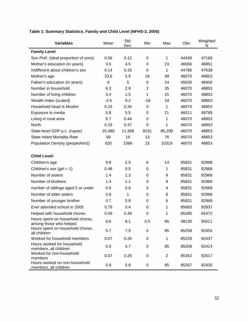
32

Table 1: Summary Statistics, Family and Child Level (NFHS-3, 2005)

Variables Mean Std. Dev. Min Max Obs Weighted

N Family Level: Son Pref. (ideal proportion of sons) 0.56 0.12 0 1 44349 47168 Mother's education (in years) 3.5 4.5 0 23 46066 48851 Indifferent about children's sex 0.14 0.33 0 1 44786 47638 Mother's age 33.6 5.9 18 49 46070 48853 Father's education (in years) 6 5 0 24 45630 48405 Number in household 6.3 2.9 2 35 46070 48853 Number of living children 3.4 1.5 1 15 46070 48853 Wealth index (scaled) -3.5 9.2 -18 24 46070 48853 Household head is Muslim 0.15 0.34 0 1 46070 48853 Exposure to media 5.8 5.5 0 21 46011 48789 Living in rural area 0.7 0.44 0 1 46070 48853 North 0.33 0.47 0 1 46070 48853 State-level GDP p.c. (rupee) 25,480 11,368 8151 85,299 46070 48853 State Infant Mortality Rate 56 16 13 76 46070 48853 Population Density (people/km2) 620 1066 15 10319 46070 48853 Child Level: Children's age 9.8 2.5 6 14 85831 92968 Children's sex (girl = 1) 0.48 0.5 0 1 85831 92968 Number of sisters 1.4 1.3 0 9 85831 92968 Number of brothers 1.4 1.1 0 9 85831 92968 number of siblings aged 5 or under 0.6 0.8 0 4 85831 92968 Number of elder sisters 0.8 1 0 8 85831 92968 Number of younger brother 0.7 0.8 0 6 85831 92968 Ever attended school in 2005 0.79 0.4 0 1 85683 92837 Helped with household chores 0.59 0.49 0 1 85285 92472 Hours spent on household chores, among those who helped 9.6 8.1 0.5 95 48130 55011

Hours spent on household chores, all children 5.7 7.9 0 95 85258 92455

Worked for household members 0.07 0.26 0 1 85228 92437 Hours worked for household members, all children 0.9 4.7 0 95 85208 92414

Worked for non-household members 0.07 0.26 0 2 85342 92517

Hours worked on non-household members, all children 0.9 5.8 0 95 85267 92435

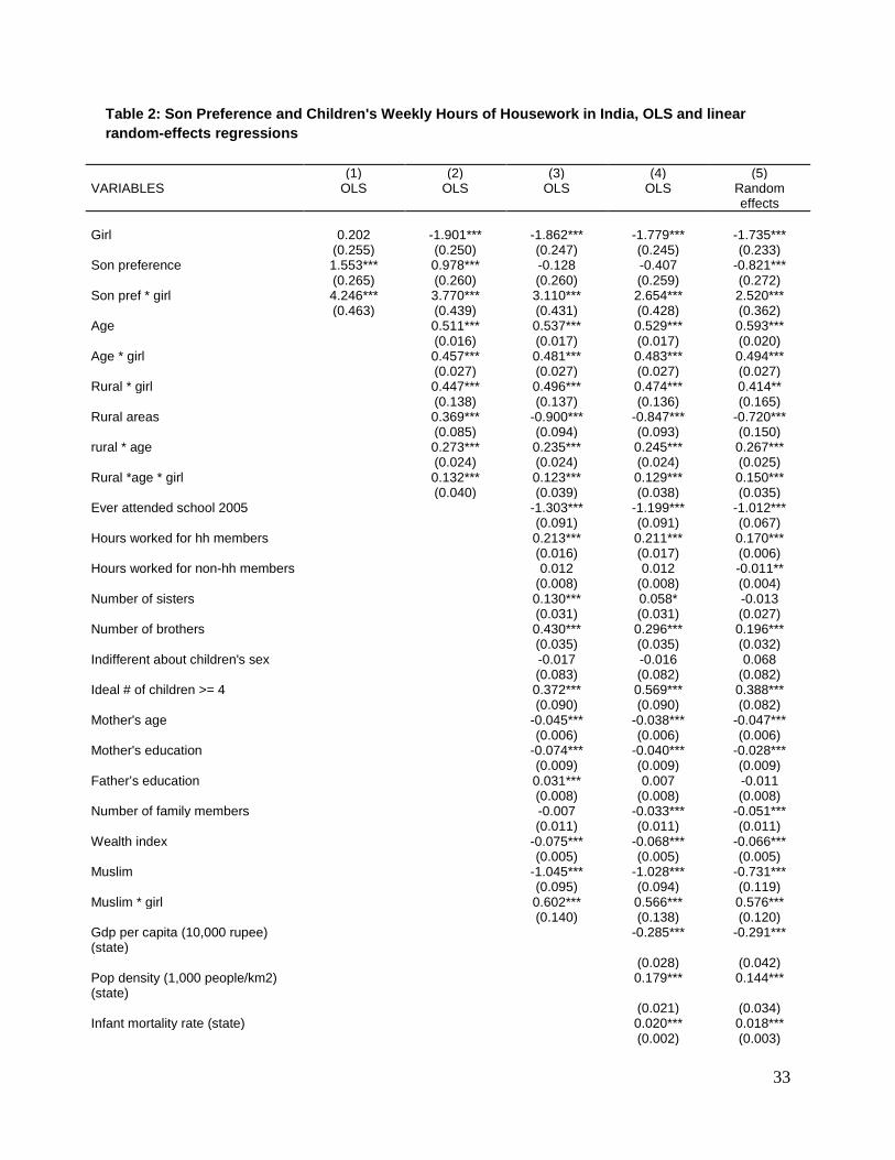
33

Table 2: Son Preference and Children's Weekly Hours of Housework in India, OLS and linear random-effects regressions

(1) (2) (3) (4) (5) VARIABLES OLS OLS OLS OLS Random

effects Girl 0.202 -1.901*** -1.862*** -1.779*** -1.735*** (0.255) (0.250) (0.247) (0.245) (0.233) Son preference 1.553*** 0.978*** -0.128 -0.407 -0.821*** (0.265) (0.260) (0.260) (0.259) (0.272) Son pref * girl 4.246*** 3.770*** 3.110*** 2.654*** 2.520*** (0.463) (0.439) (0.431) (0.428) (0.362) Age 0.511*** 0.537*** 0.529*** 0.593*** (0.016) (0.017) (0.017) (0.020) Age * girl 0.457*** 0.481*** 0.483*** 0.494*** (0.027) (0.027) (0.027) (0.027) Rural * girl 0.447*** 0.496*** 0.474*** 0.414** (0.138) (0.137) (0.136) (0.165) Rural areas 0.369*** -0.900*** -0.847*** -0.720*** (0.085) (0.094) (0.093) (0.150) rural * age 0.273*** 0.235*** 0.245*** 0.267*** (0.024) (0.024) (0.024) (0.025) Rural *age * girl 0.132*** 0.123*** 0.129*** 0.150*** (0.040) (0.039) (0.038) (0.035) Ever attended school 2005 -1.303*** -1.199*** -1.012*** (0.091) (0.091) (0.067) Hours worked for hh members 0.213*** 0.211*** 0.170*** (0.016) (0.017) (0.006) Hours worked for non-hh members 0.012 0.012 -0.011** (0.008) (0.008) (0.004) Number of sisters 0.130*** 0.058* -0.013 (0.031) (0.031) (0.027) Number of brothers 0.430*** 0.296*** 0.196*** (0.035) (0.035) (0.032) Indifferent about children's sex -0.017 -0.016 0.068 (0.083) (0.082) (0.082) Ideal # of children >= 4 0.372*** 0.569*** 0.388*** (0.090) (0.090) (0.082) Mother's age -0.045*** -0.038*** -0.047*** (0.006) (0.006) (0.006) Mother's education -0.074*** -0.040*** -0.028*** (0.009) (0.009) (0.009) Father’s education 0.031*** 0.007 -0.011 (0.008) (0.008) (0.008) Number of family members -0.007 -0.033*** -0.051*** (0.011) (0.011) (0.011) Wealth index -0.075*** -0.068*** -0.066*** (0.005) (0.005) (0.005) Muslim -1.045*** -1.028*** -0.731*** (0.095) (0.094) (0.119) Muslim * girl 0.602*** 0.566*** 0.576*** (0.140) (0.138) (0.120) Gdp per capita (10,000 rupee) (state)

-0.285*** -0.291***

(0.028) (0.042) Pop density (1,000 people/km2) (state)

0.179*** 0.144***

(0.021) (0.034) Infant mortality rate (state) 0.020*** 0.018*** (0.002) (0.003)

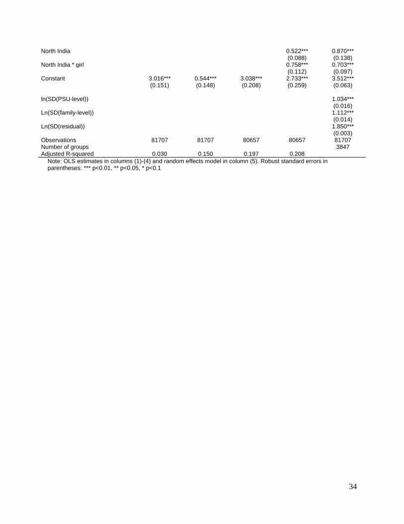
34

North India 0.522*** 0.870*** (0.088) (0.138) North India * girl 0.758*** 0.703*** (0.112) (0.097) Constant 3.016*** 0.544*** 3.038*** 2.733*** 3.512*** (0.151) (0.148) (0.208) (0.259) (0.063) ln(SD(PSU-level)) 1.034*** (0.016) Ln(SD(family-level)) 1.112*** (0.014) Ln(SD(residual)) 1.850*** (0.003) Observations 81707 81707 80657 80657 81707 Number of groups 3847 Adjusted R-squared 0.030 0.150 0.197 0.208

Note: OLS estimates in columns (1)-(4) and random effects model in column (5). Robust standard errors in parentheses: *** p<0.01, ** p<0.05, * p<0.1

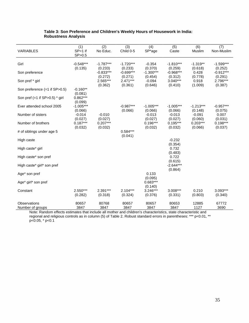
35

Table 3: Son Preference and Children's Weekly Hours of Housework in India: Robustness Analysis

(1) (2) (3) (4) (5) (6) (7) VARIABLES SP=1 if

SP>0.5 No Educ. Child 0-5 SP*age Caste Muslim Non-Muslim

Girl -0.548*** -1.787*** -1.720*** -0.354 -1.810*** -1.319** -1.599*** (0.135) (0.233) (0.233) (0.370) (0.259) (0.618) (0.252) Son preference -0.833*** -0.699*** -1.300*** -0.968*** 0.428 -0.912*** (0.272) (0.271) (0.454) (0.312) (0.778) (0.291) Son pref * girl 2.565*** 2.471*** -0.094 3.040*** 0.918 2.796*** (0.362) (0.361) (0.646) (0.410) (1.009) (0.387) Son preference (=1 if SP>0.5) -0.160** (0.081) Son pref (=1 if SP>0.5) * girl 0.862*** (0.099) Ever attended school 2005 -1.005*** -0.987*** -1.005*** -1.005*** -1.213*** -0.957*** (0.066) (0.066) (0.066) (0.066) (0.148) (0.075) Number of sisters -0.014 -0.010 -0.013 -0.013 -0.091 0.007 (0.027) (0.027) (0.027) (0.027) (0.060) (0.031) Number of brothers 0.187*** 0.207*** 0.196*** 0.195*** 0.203*** 0.198*** (0.032) (0.032) (0.032) (0.032) (0.066) (0.037) # of siblings under age 5 0.584*** (0.041) High caste -0.232 (0.354) High caste* girl 0.732 (0.483) High caste* son pref 0.722 (0.615) High caste* girl* son pref -2.644*** (0.864) Age* son pref 0.133 (0.095) Age* girl* son pref 0.683*** (0.140) Constant 2.550*** 2.391*** 2.104*** 3.246*** 3.008*** 0.210 3.093*** (0.282) (0.318) (0.324) (0.376) (0.331) (0.803) (0.340) Observations 80657 80768 80657 80657 80653 12885 67772 Number of groups 3847 3847 3847 3847 3847 1127 3690

Note: Random effects estimates that include all mother and children’s characteristics, state characteristic and regional and religious controls as in column (5) of Table 2. Robust standard errors in parentheses: *** p<0.01, ** p<0.05, * p<0.1

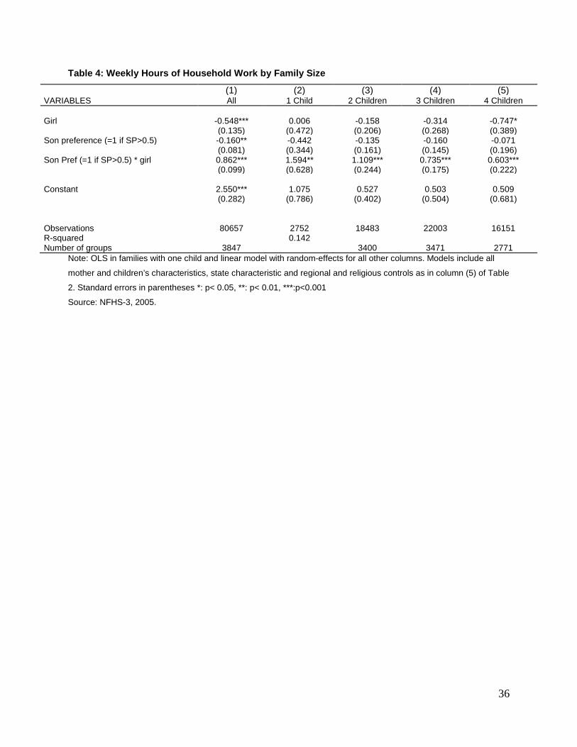
36

Table 4: Weekly Hours of Household Work by Family Size

(1) (2) (3) (4) (5) VARIABLES All 1 Child 2 Children 3 Children 4 Children Girl -0.548*** 0.006 -0.158 -0.314 -0.747* (0.135) (0.472) (0.206) (0.268) (0.389) Son preference (=1 if SP>0.5) -0.160** -0.442 -0.135 -0.160 -0.071 (0.081) (0.344) (0.161) (0.145) (0.196) Son Pref (=1 if SP>0.5) * girl 0.862*** 1.594** 1.109*** 0.735*** 0.603*** (0.099) (0.628) (0.244) (0.175) (0.222) Constant 2.550*** 1.075 0.527 0.503 0.509 (0.282) (0.786) (0.402) (0.504) (0.681) Observations 80657 2752 18483 22003 16151 R-squared 0.142 Number of groups 3847 3400 3471 2771

Note: OLS in families with one child and linear model with random-effects for all other columns. Models include all

mother and children’s characteristics, state characteristic and regional and religious controls as in column (5) of Table

2. Standard errors in parentheses *: p< 0.05, **: p< 0.01, ***:p<0.001

Source: NFHS-3, 2005.

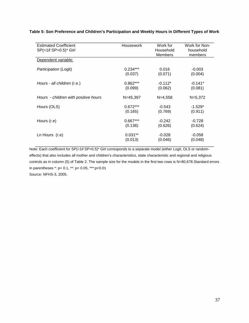
37

Table 5: Son Preference and Children’s Participation and Weekly Hours in Different Types of Work

Estimated Coefficient SP(=1if SP>0.5)* Girl

Housework Work for Household Members

Work for Non-household members

Dependent variable: Participation (Logit) 0.234*** 0.016 -0.003 (0.037) (0.071) (0.004) Hours - all children (r.e.) 0.862*** -0.112* -0.141* (0.099) (0.062) (0.081) Hours - children with positive hours N=45,397 N=4,558 N=5,372 Hours (OLS) 0.672*** -0.543 -1.529* (0.165) (0.769) (0.911) Hours (r.e) 0.667*** -0.242 -0.728 (0.136) (0.626) (0.624) Ln Hours (r.e) 0.031** -0.028 -0.058 (0.013) (0.046) (0.048)

Note: Each coefficient for SP(=1if SP>0.5)* Girl corresponds to a separate model (either Logit, OLS or random-

effects) that also includes all mother and children’s characteristics, state characteristic and regional and religious

controls as in column (5) of Table 2. The sample size for the models in the first two rows is N=80,678.Standard errors

in parentheses *: p< 0.1, **: p< 0.05, ***:p<0.01

Source: NFHS-3, 2005.

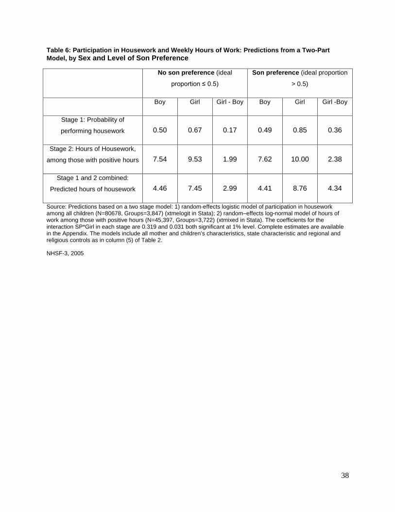
38

Table 6: Participation in Housework and Weekly Hours of Work: Predictions from a Two-Part Model, by Sex and Level of Son Preference

No son preference (ideal

proportion ≤ 0.5)

Son preference (ideal proportion

> 0.5)

Boy Girl Girl - Boy Boy Girl Girl -Boy

Stage 1: Probability of

performing housework 0.50 0.67 0.17 0.49 0.85 0.36

Stage 2: Hours of Housework,

among those with positive hours 7.54 9.53 1.99 7.62 10.00 2.38

Stage 1 and 2 combined:

Predicted hours of housework 4.46 7.45 2.99 4.41 8.76 4.34

Source: Predictions based on a two stage model: 1) random-effects logistic model of participation in housework among all children (N=80678, Groups=3,847) (xtmelogit in Stata); 2) random–effects log-normal model of hours of work among those with positive hours (N=45,397, Groups=3,722) (xtmixed in Stata). The coefficients for the interaction SP*Girl in each stage are 0.319 and 0.031 both significant at 1% level. Complete estimates are available in the Appendix. The models include all mother and children’s characteristics, state characteristic and regional and religious controls as in column (5) of Table 2.

NHSF-3, 2005

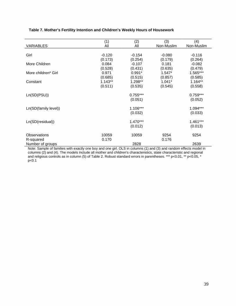
39

Table 7. Mother’s Fertility Intention and Children’s Weekly Hours of Housework

(1) (2) (3) (4) VARIABLES All All Non-Muslim Non-Muslim Girl -0.120 -0.154 -0.080 -0.116 (0.173) (0.254) (0.179) (0.264) More Children 0.084 -0.107 0.181 -0.082 (0.528) (0.431) (0.635) (0.479) More children* Girl 0.971 0.991* 1.547* 1.565*** (0.685) (0.515) (0.857) (0.585) Constant 1.143** 1.298** 1.041* 1.164** (0.511) (0.535) (0.545) (0.558) Ln(SD(PSU)) 0.755*** 0.759*** (0.051) (0.052) Ln(SD(family level)) 1.106*** 1.094*** (0.032) (0.033) Ln(SD(residual)) 1.470*** 1.461*** (0.012) (0.013) Observations 10059 10059 9254 9254 R-squared 0.170 0.176 Number of groups 2828 2639 Note: Sample of families with exactly one boy and one girl. OLS in columns (1) and (3) and random effects model in columns (2) and (4). The models include all mother and children’s characteristics, state characteristic and regional and religious controls as in column (5) of Table 2. Robust standard errors in parentheses. *** p<0.01, ** p<0.05, * p<0.1

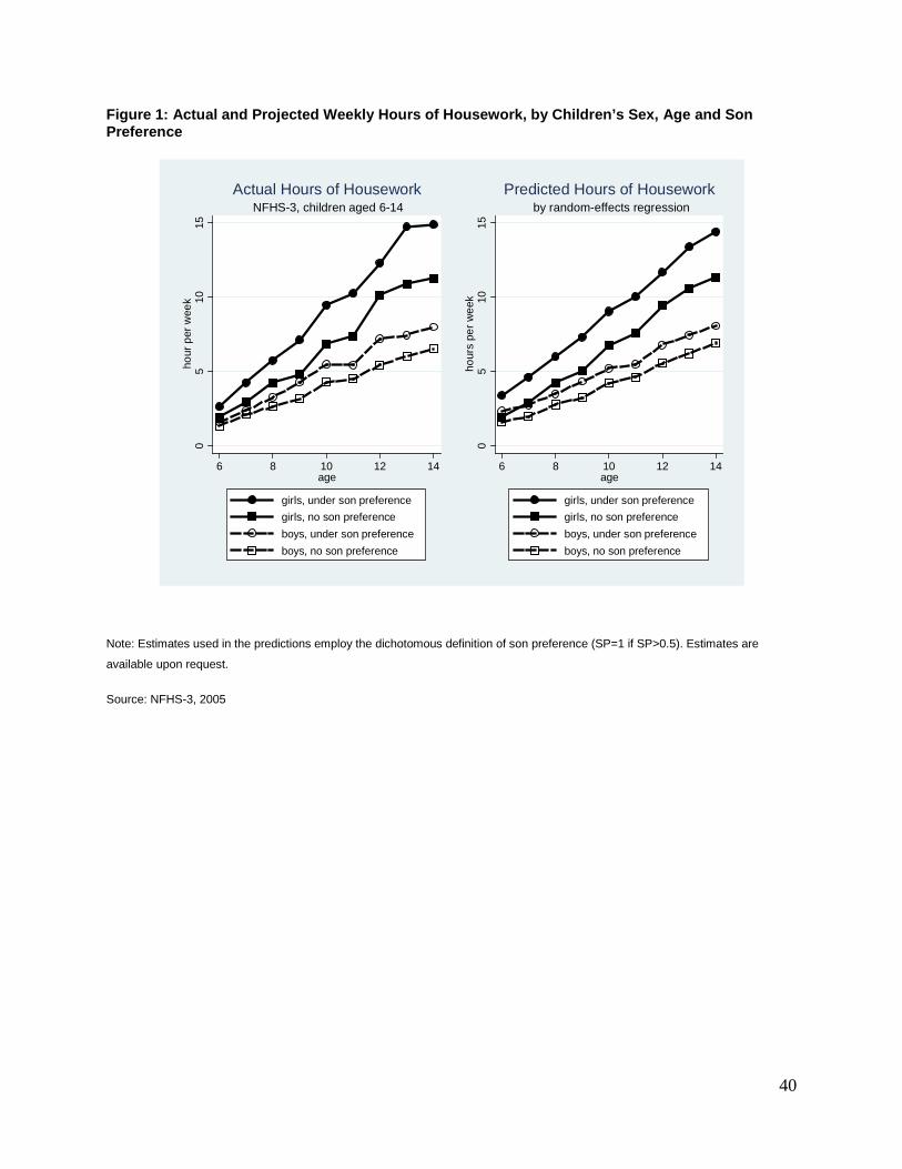
40

Figure 1: Actual and Projected Weekly Hours of Housework, by Children’s Sex, Age and Son Preference

05

1015

hour

per

wee

k

6 8 10 12 14age

girls, under son preferencegirls, no son preferenceboys, under son preferenceboys, no son preference

NFHS-3, children aged 6-14Actual Hours of Housework

05

1015

hour

s pe

r wee

k6 8 10 12 14

age

girls, under son preferencegirls, no son preferenceboys, under son preferenceboys, no son preference

by random-effects regressionPredicted Hours of Housework

Note: Estimates used in the predictions employ the dichotomous definition of son preference (SP=1 if SP>0.5). Estimates are

available upon request.

Source: NFHS-3, 2005

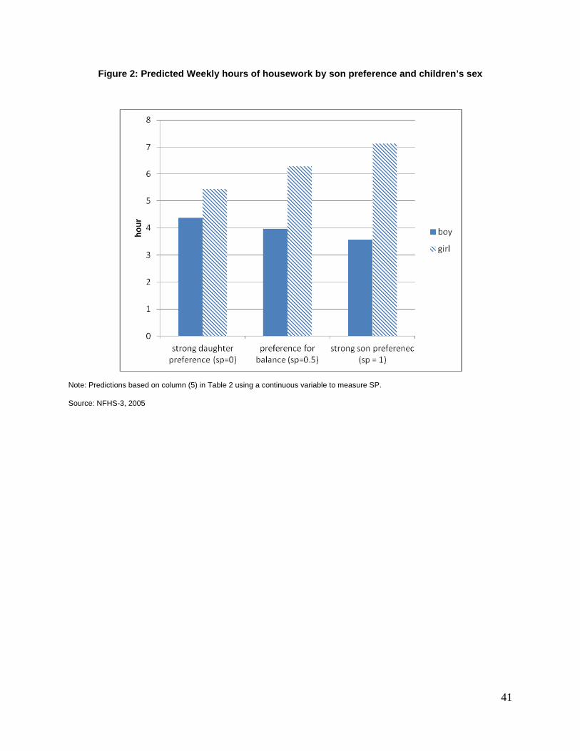
41

Figure 2: Predicted Weekly hours of housework by son preference and children’s sex

Note: Predictions based on column (5) in Table 2 using a continuous variable to measure SP.

Source: NFHS-3, 2005

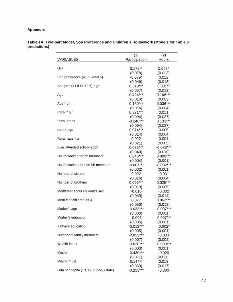
42

Appendix

Table 1A: Two-part Model, Son Preference and Children’s Housework (Models for Table 6 predictions)

(1) (2) VARIABLES Participation Hours Girl 0.176** 0.043* (0.078) (0.023) Son preference (=1 if SP>0.5) -0.079* 0.012 (0.046) (0.013) Son pref (=1 if SP>0.5) * girl 0.319*** 0.031** (0.057) (0.013) Age 0.424*** 0.108*** (0.013) (0.003) Age * girl 0.180*** 0.036*** (0.016) (0.004) Rural * girl 0.321*** 0.011 (0.094) (0.027) Rural areas -0.246*** 0.133*** (0.094) (0.027) rural * age 0.074*** 0.005 (0.014) (0.004) Rural *age * girl 0.022 0.001 (0.021) (0.005) Ever attended school 2005 0.635*** -0.088*** (0.040) (0.010) Hours worked for hh members 0.048*** 0.009*** (0.004) (0.001) Hours worked for non-hh members -0.007*** -0.002*** (0.002) (0.001) Number of sisters 0.022 -0.001 (0.016) (0.004) Number of brothers 0.095*** 0.025*** (0.019) (0.005) Indifferent about children's sex -0.010 -0.002 (0.049) (0.014) Ideal # of children >= 4 0.077 0.063*** (0.050) (0.013) Mother's age -0.033*** -0.007*** (0.003) (0.001) Mother's education -0.006 -0.007*** (0.005) (0.001) Father’s education -0.013*** -0.002* (0.005) (0.001) Number of family members -0.053*** -0.003 (0.007) (0.002) Wealth index -0.038*** -0.009*** (0.003) (0.001) Muslim -0.430*** -0.020 (0.071) (0.020) Muslim * girl 0.144** 0.013 (0.069) (0.017) Gdp per capita (10,000 rupee) (state) -0.255*** -0.000

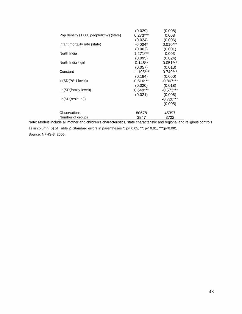
43

(0.029) (0.008) Pop density (1,000 people/km2) (state) 0.273*** 0.008 (0.024) (0.006) Infant mortality rate (state) -0.004* 0.010*** (0.002) (0.001) North India 1.271*** 0.003 (0.095) (0.024) North India * girl 0.145** 0.051*** (0.057) (0.013) Constant -1.195*** 0.749*** (0.184) (0.050) ln(SD(PSU-level)) 0.516*** -0.867*** (0.020) (0.018) Ln(SD(family-level)) 0.649*** -0.573*** (0.021) (0.008) Ln(SD(residual)) -0.720*** (0.005) Observations 80678 45397 Number of groups 3847 3722

Note: Models include all mother and children’s characteristics, state characteristic and regional and religious controls

as in column (5) of Table 2. Standard errors in parentheses *: p< 0.05, **: p< 0.01, ***:p<0.001

Source: NFHS-3, 2005.

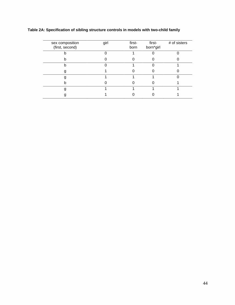
44

Table 2A: Specification of sibling structure controls in models with two-child family

sex composition (first, second)

girl first-born

first-born*girl

# of sisters

b 0 1 0 0 b 0 0 0 0 b 0 1 0 1 g 1 0 0 0 g 1 1 1 0 b 0 0 0 1 g 1 1 1 1 g 1 0 0 1

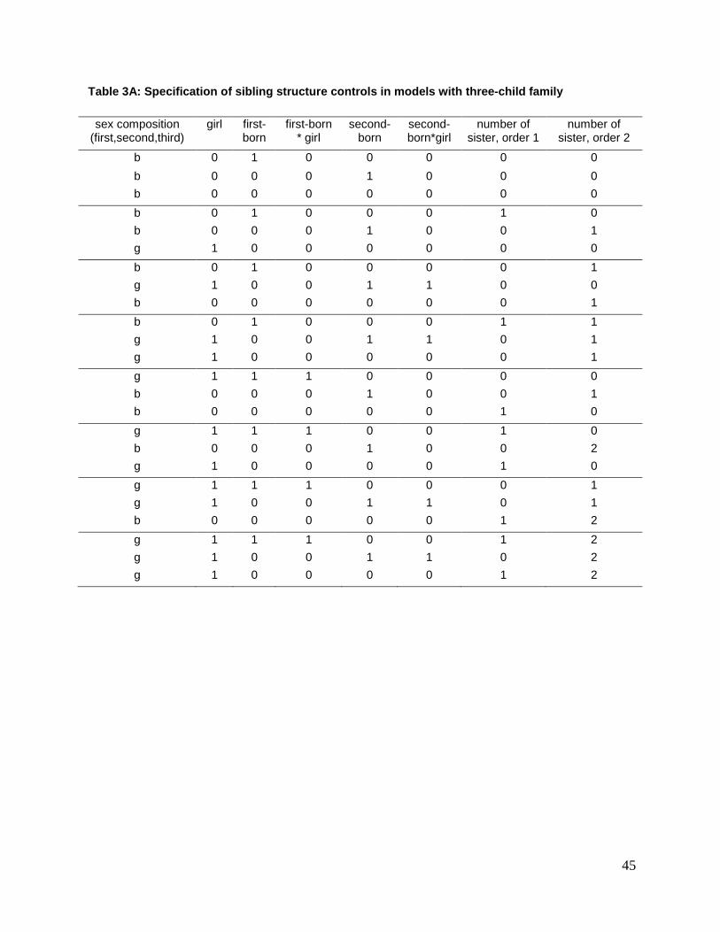
45

Table 3A: Specification of sibling structure controls in models with three-child family

sex composition (first,second,third)

girl first-born

first-born * girl

second-born

second-born*girl

number of sister, order 1

number of sister, order 2

b 0 1 0 0 0 0 0 b 0 0 0 1 0 0 0 b 0 0 0 0 0 0 0 b 0 1 0 0 0 1 0 b 0 0 0 1 0 0 1 g 1 0 0 0 0 0 0 b 0 1 0 0 0 0 1 g 1 0 0 1 1 0 0 b 0 0 0 0 0 0 1 b 0 1 0 0 0 1 1 g 1 0 0 1 1 0 1 g 1 0 0 0 0 0 1 g 1 1 1 0 0 0 0 b 0 0 0 1 0 0 1 b 0 0 0 0 0 1 0 g 1 1 1 0 0 1 0 b 0 0 0 1 0 0 2 g 1 0 0 0 0 1 0 g 1 1 1 0 0 0 1 g 1 0 0 1 1 0 1 b 0 0 0 0 0 1 2 g 1 1 1 0 0 1 2 g 1 0 0 1 1 0 2 g 1 0 0 0 0 1 2