Download - Run-time Predictive Modeling of Power and Performance via Time-Series in High Performance

Run-time Predictive Modeling of Power and Performance via Time-Series
in High Performance Computing
by
Reza Zamani
A thesis submitted to the Department of Electrical and Computer Engineering
in conformity with the requirements for
the degree of Doctor of Philosophy
Queen’s University
Kingston, Ontario, Canada
November 2012
Copyright © Reza Zamani, 2012

ABSTRACT
Pressing demands for less power consumption of processors while delivering higher perfor-
mance levels have put an extra attention on efficiency of the systems. Efficient management
of resources in the current computing systems, given their increasing number of entities and
complexity, requires accurate predictive models that can easily adapt to system and application
changes. Through performance monitoring counter (PMC) events, in modern processors, a vast
amount of information can be obtained from the system. This thesis provides a methodology
to efficiently choose such events for power modeling purposes. In addition, exploiting the
time-dependence of the data measured through PMCs and multi-meters, we build predictive
multivariate time-series models that estimate the run-time power consumption of a system. In
particular, we find an autoregressive moving average with exogenous inputs (ARMAX) model
that is combined with a recursive least squares (RLS) algorithm as a good candidate for such
purposes.
Many of the available estimation or prediction models avoid using the metrics that are
affected by the changes of the processor frequency. This thesis proposes a method to mitigate
the impact of frequency scaling in a run-time model on power and PMC metrics. This method is
based on a practical Gaussian approximation. Different segments of the trend of a metric that
are associated with different frequencies are scaled and offset into a zero mean unit variance
signal. This is an attempt to transform the variable frequency trend into a weakly stationary
time-series. Using this approach, we have shown that power estimation of a system using PMCs
can be done in a variable frequency environment.
We extend the ARMAX-RLS model to predict the near future power consumption and
PMCs of different applications in a variable frequency environment. The proposed method is
adaptive, independent of the system and applications. We have shown that a run-time per core
or aggregate system PMC event prediction, multiple-steps ahead of time, is feasible using an
ARMAX-RLS model. This is crucial for progressing from the reactive power and performance
management methods to more proactive algorithms.
ii

ACKNOWLEDGMENTS
First, I would like to thank my supervisor, Dr. Ahmad Afsahi, for his valuable feedback and
support throughout this work. His support, diligence, and commitment to high-quality research
has contributed significantly to this thesis. I am also grateful to Dr. Carl Hamacher for
supporting this work as my co-supervisor during a part of my degree. I am thankful to my Ph.D.
committee members, Dr. John Cartledge, Dr. James R. Green, Dr. Mohamed Ibnkahla, and Dr.
Mohammad Zulkernine for their insightful comments on this work.
I would like to thank my friends at the Parallel Processing Research Laboratory (PPRL),
Ying Qian, Mohammad Javad Rashti, Ryan E. Grant, Grigori Inozemtsev, Judicael A. Zounmevo,
Jonathan Green, Iman Faraji, Hessam Mirsadeghi, Ryan P. Anderson, Mike Mallin, Manju Paul
Vattathara, and Nathan R. Fredrickson, for their expert advice, research discussions, and
collaborations. I have learned a lot from each of them. Our friendships have made my time
at PPRL an enjoyable and unique experience. I am also grateful for support of the staff at
Department of Electrical and Computer Engineering (ECE). Special thanks to Debie Fraser and
Bernice Ison, ECE graduate program assistants. Special thanks to Rose Silva at School of
Graduate Studies.
I would like to acknowledge and appreciate the financial support from Ontario Graduate
Scholarship (OGS), Sun Microsystems of Canada HPCVL Research Scholarship, and Queen’s
University Student Awards. I appreciate the financial support of Natural Sciences and En-
gineering Research Council of Canada (NSERC) through some of the research assistantship
opportunities. In addition, I would like to thank Government of Ontario and Government of
Canada for providing financial assistance through Ontario Student Assistance Program (OSAP)
for completion of this work.
During my graduate studies, I have been blessed and honored for having amazing
friends that are an infinite source of inspiration, encouragement, support, and happiness for
me. Special thanks, in alphabetical order, to Nazanin Alavi, Nika Alavi, Scott Amiss, Maria
Barbero, James Chou, Guillaume Dupriez, Tiago Falk, Deborah Geist, Bahman Gharesifard,
Amir Ghasemi, Babak Hendizadeh, Parnam Izadpanah, Tarek Khalifa, Hesam Khoshneviss, Sina
iii

Khosravi, Azadeh Moghtaderi, Ali Naji Almassi, Mehrzad Namazi, Mohsen Omrani, Jennifer
Rae, Reza Rashidifar, Charlene Salazar, Sarah Salehi, Constantin Siriteanu, Maryam Soleymani,
Abd-Elhamid M. Taha, Sina Tahamtan, Amir Tahmasebi, Saeed Varziri, Davood Yazdani, and
Shahram Yousefi.
Finally, I would like to express my love and appreciation to my family. Many special and
sincere thanks go to my beautiful and understanding Kate, for her endless love, continuous
support, much needed encouragements, and kindness. I have been privileged to have her
on my side during the completion of this thesis. I am looking forward to cherishing many
future moments with her around the world. Special thanks go to my sister, Farnaz, for her
never-ending love and support throughout my life and studies. I cannot find words to express
my immense gratitude towards my parents, Masoumeh and Kazem. I am eternally indebted to
them for their sincere love and invaluable sacrifices in supporting my endeavors throughout
my life. I humbly dedicate this thesis to my parents.
iv

Table of Contents
List of Tables viii
List of Figures x
Glossary xiii
1 Introduction 1
1.1 Motivations . . . . . . . . . . . . . . . . . . . . . . . . . . . . . . . . . . . . . . . . . . . . 1
1.2 Problem Statement . . . . . . . . . . . . . . . . . . . . . . . . . . . . . . . . . . . . . . . 5
1.3 Contributions . . . . . . . . . . . . . . . . . . . . . . . . . . . . . . . . . . . . . . . . . . . 6
1.4 Dissertation Outline . . . . . . . . . . . . . . . . . . . . . . . . . . . . . . . . . . . . . . . 8
2 Background 9
2.1 Parallelism and High Performance Computing . . . . . . . . . . . . . . . . . . . . . . 9
2.2 Performance Monitoring Counters . . . . . . . . . . . . . . . . . . . . . . . . . . . . . . 12
2.3 Power Consumption . . . . . . . . . . . . . . . . . . . . . . . . . . . . . . . . . . . . . . . 13
2.4 DVFS, Clock Throttling, and DCT . . . . . . . . . . . . . . . . . . . . . . . . . . . . . . . 13
2.5 Resource Management and Related Models . . . . . . . . . . . . . . . . . . . . . . . . 14
2.5.1 Processor-Level . . . . . . . . . . . . . . . . . . . . . . . . . . . . . . . . . . . . . . 16
2.5.2 System-Level . . . . . . . . . . . . . . . . . . . . . . . . . . . . . . . . . . . . . . . 17
2.6 Applications . . . . . . . . . . . . . . . . . . . . . . . . . . . . . . . . . . . . . . . . . . . . 19
3 Performance Monitoring Counter Selection 21
3.1 Related Work . . . . . . . . . . . . . . . . . . . . . . . . . . . . . . . . . . . . . . . . . . . 22
3.2 Experimental Framework . . . . . . . . . . . . . . . . . . . . . . . . . . . . . . . . . . . . 23
3.2.1 Hardware Platform . . . . . . . . . . . . . . . . . . . . . . . . . . . . . . . . . . . 23
v

3.2.2 CentOS Software Configuration . . . . . . . . . . . . . . . . . . . . . . . . . . . . 24
3.3 Mathematical Review . . . . . . . . . . . . . . . . . . . . . . . . . . . . . . . . . . . . . . 25
3.4 Measurement Variability . . . . . . . . . . . . . . . . . . . . . . . . . . . . . . . . . . . . 25
3.5 Single PMC Selection . . . . . . . . . . . . . . . . . . . . . . . . . . . . . . . . . . . . . . 31
3.5.1 Correlation in Event Space . . . . . . . . . . . . . . . . . . . . . . . . . . . . . . . 32
3.5.2 Rank in Application Space . . . . . . . . . . . . . . . . . . . . . . . . . . . . . . . 32
3.6 Multiple PMC Selection . . . . . . . . . . . . . . . . . . . . . . . . . . . . . . . . . . . . . 33
3.6.1 Sub-Space Projection Method . . . . . . . . . . . . . . . . . . . . . . . . . . . . . 37
3.6.2 Results . . . . . . . . . . . . . . . . . . . . . . . . . . . . . . . . . . . . . . . . . . . 39
3.7 Discussion . . . . . . . . . . . . . . . . . . . . . . . . . . . . . . . . . . . . . . . . . . . . . 41
4 Fixed Frequency Power Estimation 45
4.1 Related Work . . . . . . . . . . . . . . . . . . . . . . . . . . . . . . . . . . . . . . . . . . . 46
4.2 Models and Algorithms . . . . . . . . . . . . . . . . . . . . . . . . . . . . . . . . . . . . . 48
4.2.1 ARMAX . . . . . . . . . . . . . . . . . . . . . . . . . . . . . . . . . . . . . . . . . . . 48
4.2.2 Discrete-Time Kalman Filter . . . . . . . . . . . . . . . . . . . . . . . . . . . . . . 49
4.2.3 Recursive Least-Squares Filter . . . . . . . . . . . . . . . . . . . . . . . . . . . . 51
4.2.4 System Identification using KF . . . . . . . . . . . . . . . . . . . . . . . . . . . . 52
4.3 Experimental Framework . . . . . . . . . . . . . . . . . . . . . . . . . . . . . . . . . . . . 54
4.3.1 Ubuntu Software Setup . . . . . . . . . . . . . . . . . . . . . . . . . . . . . . . . . 55
4.4 Time-Series . . . . . . . . . . . . . . . . . . . . . . . . . . . . . . . . . . . . . . . . . . . . 55
4.4.1 Power Estimation Model . . . . . . . . . . . . . . . . . . . . . . . . . . . . . . . . 56
4.5 Simulation Results of Real System Measurements . . . . . . . . . . . . . . . . . . . . 58
4.5.1 Error Reporting . . . . . . . . . . . . . . . . . . . . . . . . . . . . . . . . . . . . . 59
4.5.2 Coefficient Update Algorithms . . . . . . . . . . . . . . . . . . . . . . . . . . . . 60
4.5.3 Computation-time Overhead . . . . . . . . . . . . . . . . . . . . . . . . . . . . . 61
4.5.4 Sensitivity to Measurement Update Delay . . . . . . . . . . . . . . . . . . . . . 61
4.5.5 PMC Selection and Filter Size . . . . . . . . . . . . . . . . . . . . . . . . . . . . . 64
4.5.6 Adapting to Significant Application Changes . . . . . . . . . . . . . . . . . . . 69
4.6 Discussion . . . . . . . . . . . . . . . . . . . . . . . . . . . . . . . . . . . . . . . . . . . . . 70
vi

5 Variable Frequency Power Estimation 72
5.1 Related Work . . . . . . . . . . . . . . . . . . . . . . . . . . . . . . . . . . . . . . . . . . . 72
5.2 Effect of Variable Frequency on PMC and Power Trends . . . . . . . . . . . . . . . . . 73
5.3 Zero Mean Unit Variance Module . . . . . . . . . . . . . . . . . . . . . . . . . . . . . . . 81
5.3.1 Scale and Offset . . . . . . . . . . . . . . . . . . . . . . . . . . . . . . . . . . . . . 82
5.4 ZMUV Signal Estimation Results . . . . . . . . . . . . . . . . . . . . . . . . . . . . . . . 83
5.5 Power Estimation Results . . . . . . . . . . . . . . . . . . . . . . . . . . . . . . . . . . . 84
5.6 Discussion . . . . . . . . . . . . . . . . . . . . . . . . . . . . . . . . . . . . . . . . . . . . . 89
6 Power and Performance Prediction 90
6.1 Related Work . . . . . . . . . . . . . . . . . . . . . . . . . . . . . . . . . . . . . . . . . . . 90
6.2 Performance Prediction using ARMAX-RLS . . . . . . . . . . . . . . . . . . . . . . . . . 93
6.2.1 PMC Prediction Model . . . . . . . . . . . . . . . . . . . . . . . . . . . . . . . . . 93
6.2.2 PMC Prediction Results . . . . . . . . . . . . . . . . . . . . . . . . . . . . . . . . . 95
6.3 Power Prediction using ARMAX-RLS . . . . . . . . . . . . . . . . . . . . . . . . . . . . . 107
6.3.1 Power Prediction Model . . . . . . . . . . . . . . . . . . . . . . . . . . . . . . . . 108
6.3.2 Power Prediction Results . . . . . . . . . . . . . . . . . . . . . . . . . . . . . . . . 109
6.4 IPC Prediction in Real Time . . . . . . . . . . . . . . . . . . . . . . . . . . . . . . . . . . 114
6.4.1 Aggregate PMCs . . . . . . . . . . . . . . . . . . . . . . . . . . . . . . . . . . . . . 115
6.4.2 Per Core PMCs . . . . . . . . . . . . . . . . . . . . . . . . . . . . . . . . . . . . . . 118
6.5 Discussion . . . . . . . . . . . . . . . . . . . . . . . . . . . . . . . . . . . . . . . . . . . . . 120
7 Conclusions and Future Work 121
7.1 Future Work . . . . . . . . . . . . . . . . . . . . . . . . . . . . . . . . . . . . . . . . . . . . 123
References 124
vii

List of Tables
1.1 Top 20 supercomputers (adapted from [133] in June 2012) . . . . . . . . . . . . . . 3
3.1 List of selected PMC events for AMD Opteron processors (part I) . . . . . . . . . . . 26
3.2 List of selected PMC events for AMD Opteron processors (part II) . . . . . . . . . . 27
3.3 Mean and standard deviation of power-PMC and PMC-PMC correlation coefficients
(102 measurements) . . . . . . . . . . . . . . . . . . . . . . . . . . . . . . . . . . . . . . . 28
3.4 BT.C - Top 25 correlated events . . . . . . . . . . . . . . . . . . . . . . . . . . . . . . . . 33
3.5 CG.C - Top 25 correlated events . . . . . . . . . . . . . . . . . . . . . . . . . . . . . . . 34
3.6 LU.C - Top 25 correlated events . . . . . . . . . . . . . . . . . . . . . . . . . . . . . . . . 35
3.7 SP.C - Top 25 correlated events . . . . . . . . . . . . . . . . . . . . . . . . . . . . . . . . 36
3.8 Top 24 unified events (rank median) . . . . . . . . . . . . . . . . . . . . . . . . . . . . 37
4.1 R2, MAEDS, and MAETS of power estimation using an ARMAX with different
parameters (n, 0, m+ 1) . . . . . . . . . . . . . . . . . . . . . . . . . . . . . . . . . . . . 65
5.1 R2 and MAEDS of variable frequency ZMUV power estimation using ARMAX(4, 0,
5) and ARMAX(10, 0, 11) . . . . . . . . . . . . . . . . . . . . . . . . . . . . . . . . . . . . 84
5.2 R2, MAEDS, and MAETS of variable frequency power estimation using ARMAX(4, 0, 5) 85
6.1 Efficiency of variable frequency IPC predictions . . . . . . . . . . . . . . . . . . . . . . 97
6.2 Efficiency of variable frequency Micro-architectural Early Cancel of an Access rate
predictions . . . . . . . . . . . . . . . . . . . . . . . . . . . . . . . . . . . . . . . . . . . . 97
6.3 Efficiency of variable frequency Data Cache Lines Evicted rate predictions . . . . . 98
6.4 Efficiency of variable frequency L2 Fill/Writeback rate predictions . . . . . . . . . . 98
6.5 Efficiency of variable frequency power consumption predictions . . . . . . . . . . . 110
6.6 Efficiency of variable frequency real time aggregate PMC prediction . . . . . . . . . 118
viii

6.7 Efficiency of aggregate and per core one-step ahead PMC predictions . . . . . . . . 119
ix

List of Figures
2.1 Diagram of power and performance resource management approaches . . . . . . . 15
3.1 Power measurement diagram . . . . . . . . . . . . . . . . . . . . . . . . . . . . . . . . . 24
3.2 Correlation measurement variability for BT.C . . . . . . . . . . . . . . . . . . . . . . . 29
3.3 Correlation measurement variability for CG.C . . . . . . . . . . . . . . . . . . . . . . . 29
3.4 Correlation measurement variability for LU.C . . . . . . . . . . . . . . . . . . . . . . . 30
3.5 Correlation measurement variability for SP.C . . . . . . . . . . . . . . . . . . . . . . . 30
3.6 Zero-mean normalized power variations captured by PMCs (BT.C) . . . . . . . . . . 41
3.7 Zero-mean normalized power variations captured by PMCs (CG.C) . . . . . . . . . . 42
3.8 Zero-mean normalized power variations captured by PMCs (LU.C) . . . . . . . . . . 43
3.9 Zero-mean normalized power variations captured by PMCs (SP.C) . . . . . . . . . . 43
3.10R2 for 64-sample segments . . . . . . . . . . . . . . . . . . . . . . . . . . . . . . . . . . 44
4.1 Sample autocorrelation function of the differenced power trends . . . . . . . . . . 56
4.2 Block diagram of the model and coefficient update algorithm . . . . . . . . . . . . . 57
4.3 Comparing power estimation of BT.C running with 8 threads using RLS, MVNR,
BMVNR, KF, MA-0, and Oracle models . . . . . . . . . . . . . . . . . . . . . . . . . . . . 62
4.4 MAEDS and MAETS of power estimation using different coefficient update algorithms 63
4.5 The effect of delay on MAEDS using different coefficient update algorithms . . . . 64
4.6 Power estimation of BT.C using ARMAX(20, 0, 21) . . . . . . . . . . . . . . . . . . . . 66
4.7 Power estimation of CG.C using ARMAX(20, 0, 21) . . . . . . . . . . . . . . . . . . . . 67
4.8 Power estimation of LU.C using ARMAX(20, 0, 21) . . . . . . . . . . . . . . . . . . . . 67
4.9 Power estimation of SP.C using ARMAX(20, 0, 21) . . . . . . . . . . . . . . . . . . . . 68
x

4.10 Run-time power estimation of multiple applications (extreme cases: idle period,
and start/end of a benchmark) . . . . . . . . . . . . . . . . . . . . . . . . . . . . . . . . 70
5.1 The impact of frequency changes on power consumption and PMCs of BT.C . . . . 74
5.2 Variable frequency power consumption of consecutive execution of BT.C, LU.C,
SP.C, FT.C, and MG.C . . . . . . . . . . . . . . . . . . . . . . . . . . . . . . . . . . . . . . 76
5.3 Variable frequency Micro-architectural Early Cancel of an Access (rate) of consecu-
tive execution of BT.C, LU.C, SP.C, FT.C, and MG.C . . . . . . . . . . . . . . . . . . . . 77
5.4 Variable frequency Data Cache Lines Evicted (rate) of consecutive execution of
BT.C, LU.C, SP.C, FT.C, and MG.C . . . . . . . . . . . . . . . . . . . . . . . . . . . . . . . 78
5.5 Variable frequency L2 Fill/Writeback (rate) of consecutive execution of BT.C, LU.C,
SP.C, FT.C, and MG.C . . . . . . . . . . . . . . . . . . . . . . . . . . . . . . . . . . . . . . 79
5.6 Variable frequency Retired MMX/FP Instructions (rate) of consecutive execution of
BT.C, LU.C, SP.C, FT.C, and MG.C . . . . . . . . . . . . . . . . . . . . . . . . . . . . . . . 80
5.7 Block diagram of model, coefficient update and scaling (zero mean unit variance)
modules . . . . . . . . . . . . . . . . . . . . . . . . . . . . . . . . . . . . . . . . . . . . . . 82
5.8 ZMUV signal, mean, and variance of power consumption for FT.C . . . . . . . . . . 84
5.9 ZMUV signal, mean, and variance of Micro-architectural Early Cancel of an Access
(rate) for FT.C . . . . . . . . . . . . . . . . . . . . . . . . . . . . . . . . . . . . . . . . . . . 85
5.10 Estimation of the ZMUV power signal and its equivalent in original frequencies for
BT.C . . . . . . . . . . . . . . . . . . . . . . . . . . . . . . . . . . . . . . . . . . . . . . . . . 86
5.11 Variable frequency power estimation of LU.C . . . . . . . . . . . . . . . . . . . . . . . 87
5.12 Variable frequency power estimation of SP.C . . . . . . . . . . . . . . . . . . . . . . . 87
5.13 Variable frequency power estimation of FT.C . . . . . . . . . . . . . . . . . . . . . . . 88
5.14 Variable frequency power estimation of MG.C . . . . . . . . . . . . . . . . . . . . . . . 88
6.1 One-step and two-step ahead predictions for IPC of BT.C . . . . . . . . . . . . . . . . 99
6.2 One-step and two-step ahead predictions for IPC of LU.C . . . . . . . . . . . . . . . . 99
6.3 One-step and two-step ahead predictions for IPC of SP.C . . . . . . . . . . . . . . . . 100
6.4 One-step and two-step ahead predictions for IPC of FT.C . . . . . . . . . . . . . . . . 100
6.5 One-step and two-step ahead predictions for IPC of MG.C . . . . . . . . . . . . . . . 101
xi

6.6 One-step and two-step ahead predictions for PMCs of BT.C . . . . . . . . . . . . . . 102
6.7 One-step and two-step ahead predictions for PMCs of LU.C . . . . . . . . . . . . . . 103
6.8 One-step and two-step ahead predictions for PMCs of SP.C . . . . . . . . . . . . . . . 104
6.9 One-step and two-step ahead predictions for PMCs of FT.C . . . . . . . . . . . . . . 105
6.10 One-step and two-step ahead predictions for PMCs of MG.C . . . . . . . . . . . . . . 106
6.11 One-step and two-step ahead predictions for power consumption of BT.C . . . . . 111
6.12 One-step and two-step ahead predictions for power consumption of LU.C . . . . . 111
6.13 One-step and two-step ahead predictions for power consumption of SP.C . . . . . 112
6.14 One-step and two-step ahead predictions for power consumption of FT.C . . . . . 112
6.15 One-step and two-step ahead predictions for power consumption of MG.C . . . . . 113
6.16 One-step and two-step ahead real time predictions for IPC (set 1) . . . . . . . . . . 116
6.17 One-step and two-step ahead real time predictions for IPC (set 2) . . . . . . . . . . 116
6.18 One-step and two-step ahead real time predictions for L2 Fill/Writeback (set 1) . . 117
6.19 One-step and two-step ahead real time predictions for L2 Fill/Writeback (set 2) . . 117
xii

Glossary
ACF Autocorrelation function
ACPI Advanced Configuration and Power Interface
ANOVA Analysis of Variance
API Application Programming Interface
AR Autoregressive
ARFIMA Autoregressive Fractionally Integrated Moving Average
ARIMA Autoregressive Integrated Moving Average
ARMA Autoregressive Moving Average
ARMAX Autoregressive Moving Average with Exogenous Inputs
BMVNR Block Multivariate Normal Regression
BT Block Tri-diagonal
CFD Computational Fluid Dynamics
CG Conjugate Gradient
CMOS Complementary Metal Oxide Semiconductor
CMP Chip Multi-Processing
CPI Cycles Per Instruction
CPU Central Processing Unit
DCT Dynamic Concurrency Throttling
DMM Digital Multi-Meter
DTM Dynamic Thermal Management
DVFS Dynamic Voltage and Frequency Scaling
EP Embarrassingly Parallel
FT Fourier Transform
GPU Graphical Processing Unit
xiii

HPC High-Performance Computing
HPM Hardware Performance Monitoring
HT Hyper-Threading
IC Integrated Circuit
ILP Instruction-Level Parallelism
IPC Instructions Per Cycle
IS Integer Sort
KF Kalman Filter
LU Lower-Upper
MA Moving Average
MAEDS Mean Absolute Error of Dynamic Signal
MAETS Mean Absolute Error of Total Signal
MFLOPS Mega (106) Floating Point Operations per Second
MG Multi-Grid
MLE Maximum Likelihood Estimation
MP Multi-Processor
MPI Message Passing Interface
MVNR Multivariate Normal Regression
NPB NAS Parallel Benchmark
NUMA Non-Uniform Memory Access
NWS Network Weather Service
OSPM Operating System Power Management
PCA Principal Component Analysis
PFLOPS Peta (1015) Floating Point Operations per Second
PM Power Management
PMC Performance Monitoring Counter
PMU Performance Monitoring Unit
RLS Recursive Least Squares
RPS Resource Prediction System
xiv

SIMD Single Instruction Multiple Data
SLES SUSE Linux Enterprise Server
SMM Statistical Metric Model
SMP Symmetric Multi-Processors
SMT Simultaneous Multi-Threading
SNR Signal-to-Noise Ratio
SP Scalar Penta-diagonal
TLP Thread-Level Parallelism
UA Unstructured Adaptive
VM Virtual Machine
ZMUV Zero Mean Unit Variance
xv

Chapter 1
Introduction
The thesis provides research to utilize available computing system information to obtain
effective and accurate power and performance models. Such models are essential for efficient
allocation and management of resources, given various goals, in a computing system. Power
saving, power capping, and performance enhancement are among the main goals that can
benefit from the contributions of this thesis.
This chapter provides a brief introduction to the research presented in this thesis.
Section 1.1 describes some of the motivations for this work. Section 1.2 provides a list of
problems that this thesis tries to address. Section 1.3 summarizes the main contributions of
this work. Section 1.4 outlines the organization of this thesis.
1.1 Motivations
Today’s computing industry faces two major challenges for delivering faster and more scalable
computing systems: power and performance. Performance has always been the main goal of
computing industry. However, recently, power consumption and its related issues have taken
a similar priority, if not more important [16, 107]. Computing system architects commonly
have been facing trade-offs between power consumption and performance enhancement. Heat
dissipation issues in processors, due to physical limitations, have stopped the trend of man-
ufacturing processors with higher operating frequencies. This is referred to as power wall
[43, 98] that hinders serial performance enhancement of processors. In addition, the perfor-
mance gap between memory modules and processors, which has been growing significantly,
presents an obstacle in improving serial performance of applications. This growing difference
between memory cycles and processor cycles is referred to as memory wall [145]. Furthermore,
1

instruction-level parallelism (ILP) strives for finding enough parallelism in a stream of instruc-
tions to fully utilize a high-performance single-core processor. In computing literature, this is
referred to as ILP wall [98]. The combination of power wall, memory wall, and ILP wall, among
other reasons, has fueled research and development of multi-core processors, such as dual-core
IBM Power-5 processor [77], 32-way Sparc processor [81], 12-core AMD Opteron processor [26],
48-core Intel SCC processor [60, 99], and 64-core Godson-T [40].
This thesis focuses on high-performance computing (HPC) applications. HPC is the
cornerstone of scientific community in tackling challenging problems in diverse fields such as
energy, medicine, weather and climate, finance, defense, and data mining. HPC applications rep-
resent a category of applications with one of the tightest thresholds for acceptable performance
degradation under a power saving method.
Power consumption and cooling issues of current HPC systems result in high operational
and maintenance costs. The large number of power hungry cores in modern HPC systems incur
a substantial cost of ownership [10]. Therefore, along with traditional performance-oriented
focus of industry, power consumption and cooling issues of HPC systems have become an
important part of the new design constraints. Table 1.1 shows the gravity of high power
consumption and large number of cores in today’s HPC world. For instance, Jaguar, one of
the leading systems on the Top500 list [133], recording a performance of 1.941 PFLOPS, has
298,592 cores, requiring 5.142 MW of power. Assuming a nominal cost of $0.10/kWh, this
translates into an average annual electricity cost of $4.5M. Jaguar has a performance/power
efficiency of 377 MFLOPS/Watt. This is relatively low compared to custom designed Blue Gene
systems like Sequoia with 2069 MFLOPS/Watt. Jaguar has been updated with the latest 16-Core
AMD Opteron 2.2 GHz processors, in addition to partially utilizing NVIDIA 2090 graphical
processing units (GPU). In contrast, Sequoia uses custom Blue Gene/Q, 1.6 GHz Power BQC
processors with 16 processing cores (total of 18 cores available, however, only 16 cores are
used). The race for efficiency in supercomputing has inspired maintaining an efficiency ranking
system for the top supercomputers [129].
As current state of computing industry faces diminishing results in performance en-
hancement of single-core processors, it is expected for the future systems to have many more
cores per socket (e.g., 1000 cores per socket) [59, 91]. The large number of cores in a socket
2

Table 1.1: Top 20 supercomputers (adapted from [133] in June 2012)Rank Name Total Cores Power (kW) MFLOPS/Watt Cores/Socket
1 Sequoia 1,572,864 7,890 2,069 162 K computer 705,024 12,660 830 83 Mira 786,432 3,945 2,069 164 SuperMUC 147,456 3,423 846 85 Tianhe-1A 186,368 4,040 635 66 Jaguar 298,592 5,142 377 167 Fermi 163,840 822 2,099 168 JuQUEEN 131,072 658 2,099 169 Curie thin nodes 77,184 2,251 604 810 Nebulae 120,640 2,580 493 611 Pleiades 125,980 3,987 312 412 Helios 70,560 2,200 562 813 Blue Joule 114,688 575 2,099 1614 TSUBAME 2.0 73,278 1,399 852 615 Cielo 142,272 3,980 279 816 Hopper 153,408 2,910 362 1217 Tera-100 138,368 4,590 229 818 Oakleaf-FX 76,800 1,177 886 1619 Roadrunner 122,400 2,345 444 920 DiRAC 98,304 493 2,099 16
brings in more challenges in managing resources of the system. Given the current challenges of
power and performance trade-offs, in addition to future challenges that many-core systems are
expected to introduce, it is necessary to obtain a highly efficient resource management system
to provide scalable systems with higher performance and lower power consumption.
Efficient resource management in a computing system becomes explosively difficult,
given the complexity and the number of modules in a system. This is mainly due to absence
of a simple and accurate model that can describe the behavior of the system from various
aspects. To solve this shortcoming, simple metrics, such as processor utilization, have been used
commonly as a basis for resource management and related decision makings. Two common
instances where processor utilization metric is used are the operating system scheduler and
the processor power management module (i.e., voltage and frequency governors).
In a system with a complex processor architecture running different flavors of applica-
tions, such as compute-bound, communication-bound, and memory-bound applications, there
are many reasons that make the processor utilization an inaccurate metric for resource man-
3

agement purposes [115]. Examples of such complexities for a single processor are multi-level
caches, non-uniform memory, pipelining, out-of-order execution, and simultaneous multi-
threading (SMT). In addition to complex single processor advancements, multi-core processors
and multi-CPU systems, make the CPU utilization metric less reliable for performance capacity
prediction purposes.
Modern processors provide the capability to monitor their performance events through
hardware performance monitoring counters (PMC) [125]. Some systems also provide uncore
metrics, such as read or write bytes from or to memory controllers [67]. In most common
processors, a broad group of events are available for measurement through a small number
of registers. For example, the AMD Opteron processor used in this thesis provides more than
150 events to choose from and 4 registers for each core to use for monitoring such events
simultaneously. Future generations of microprocessors are expected to have more simultaneous
counters available [116]. In computer literature, PMCs also have been referred to via other
terms such as, performance monitoring unit (PMU) [115] and hardware performance monitoring
(HPM) support [120].
Given such a vast source of information, is it possible to provide a model that is accurate,
adaptive, system-independent, application-independent, and able to estimate and predict
the state of the system in terms of power consumption and performance events? Resource
management, power saving, power capping, task scheduling, and many other management
modules can significantly benefit from such models, if they come to realization.
The goal of this thesis is to facilitate building models and metrics that accurately repre-
sent the current and future state of the system for resource management purposes. This thesis
provides a better understanding of usage of PMCs in power estimation models. Specifically, this
thesis addresses the problem of finding an optimum set of events for efficient power modeling
[152]. Furthermore, novel power estimation models that are based on multivariate time-series
analysis are presented in this work [151]. Using multivariate time-series analysis is orthogonal
to many prior work in this field. In addition to power estimation models [150], this thesis
provides models that are predictive [154] both for power consumption and PMC events in a
frequency variable environment. In short, this work provides necessary tools and models to
4

harvest valuable and accurate information to increase the efficiency of resource management
for current and future systems.
1.2 Problem Statement
Demand for efficiency in resource allocation stays at its peak in the present and future many-
core era, given the existence of trade-offs between the two important design measures, power
and performance. Current state of resource management mainly uses a reactive approach
towards system’s measured metrics. For example, current power managers of Windows Vista
and SUSE Linux Enterprise Server (SLES) adjust the frequency and voltage settings of next time
period in a reactive mode, based on the previous load [14]. Similar reactive decision makings
can be observed in schedulers [3, 5, 17]. The delay between observing a change in system’s
workload and adjusting the system’s settings, such as voltage and frequency, is inevitable in
reactive algorithms. This inherent delay in reactive methods results in a lower efficiency of
power and performance [13].
Modern processors are capable of measuring many different performance metrics
through PMCs. Predictive models for power and PMCs at run-time with a fine granularity in
time domain (many measurements, many estimations, and many predictions per second) can
significantly improve the efficiency of power and performance management modules. For
example, the adjustment of processor voltage and frequency can be trivially performed in
advance, knowing the upcoming workload performance requirements. The general conditions
that this thesis tries to follow in developing any model is accuracy, adaptiveness, application-
independence, architecture-independence, and non-intrusiveness. The primary questions that
this thesis tries to address are:
1. Given the large number of available PMC events and the small number of registers for
simultaneous measurements, what is an efficient method for finding an optimal selection
of multiple PMC events for power modeling of computing systems?
2. Under a fixed processor frequency, is it possible to use the time dependence of data to
obtain an accurate power estimation model based on PMCs? Is a multivariate time-series
5

approach beneficial for this purpose? If yes, what models and algorithms in multivariate
time-series are more efficient?
3. Given that all trends of PMCs and power consumption is affected significantly by
frequency variations, is it possible to obtain a variable frequency power estimation
model that is based on multivariate time-series analysis?
4. Are multivariate time-series models capable of predicting future PMCs and power
consumption for different frequencies of the system multiple time steps ahead?
1.3 Contributions
This section summarizes the contributions made by the work presented in this thesis. First,
this thesis studies the problem of choosing proper PMC events for a PMC-based power model.
Without relying on architectural intuitions for PMC event selections, we perform a comprehen-
sive statistical analysis of PMC events and power consumption. We verify that the variability
of power-PMC and PMC-PMC correlations are tolerable for PMC event selections. In order to
provide the power models with the most useful information from the system, through the
limited number of available PMC registers and with a minimal overlap of information provided
by different measured PMC events, this thesis proposes an optimized method for selection of
multiple PMCs. The proposed method requires six times fewer executions of an application than
a principal component analysis method, without the assumption that the statistics of power
consumption and PMCs for different processes or threads of a parallel application are identical
among different cores or nodes. The presented results in Chapter 3 are for power models using
PMCs, however, this method can be adapted to the needs of one who seeks a linear model
between PMCs and other objectives, such as temperature-related and performance-related
metrics.
This thesis proposes a power estimation model that is based on multivariate time-series
analysis, in particular, autoregressive moving average with exogenous input model (ARMAX).
A multivariate time-series model exploits the intrinsic repetitiveness of computer software
and hardware activities through the time dependence in a power or PMC signal or between
power and PMC signals. We have shown that using the time dependence improves the power
6

estimation models significantly. In order to obtain an ARMAX model that is able to adapt
to the changes in a system, in addition to being architecture- and application-independent,
it is equipped with a coefficient update algorithm. This thesis evaluates the effectiveness of
applying different coefficient update algorithms to the ARMAX models, such as multivariate
normal regression (MVNR), Kalman filter (KF), and recursive least squares (RLS). This thesis
studies different aspects of an ARMAX power estimation model, such as computation-time
overhead, sensitivity to measurement update delay, PMC selection, filter size, and adaptation
to significant application changes. Based on the minimal computational overhead and the
superior performance of th RLS algorithm, we adopt ARMAX-RLS as the preferred model for the
rest of this thesis (Chapter 5 and Chapter 6). The research in Chapter 4 is limited to a fixed
processor frequency and does not account for the variations in power and PMC trends of a
variable frequency environment.
The unknown scaling of PMC and power metrics as a result of frequency scaling cripples
the integration of many existing models into a real system. This thesis studies the effect of
frequency scaling on power and PMC signals and proposes a method to prepare those signals
for usage in a multivariate time-series power estimation model. In particular, the proposed
method is based on a practical Gaussian approximation, and it does not rely on differentiating
between the scaling and the non-scaling metrics. The proposed method is a general approach
for different PMC and power signals. Unlike the prior works, the proposed method is not limited
to a small set of PMC events that follows an architectural model. This approach scales and
offsets the metrics by their mean and variance associated to each frequency into a unified trend
with a zero mean and unit variance (ZMUV). It is demonstrated in Chapter 5 that an ARMAX
model, equipped with the RLS algorithm and the ZMUV module, can accurately estimate the
power consumption of a real system in a variable frequency environment.
Furthermore, we propose a model based on the ARMAX-RLS model to predict the future
PMC and power consumption values in a variable frequency environment. This method is a
general approach to PMC event rate and power consumption prediction, and unlike the prior
works it is not limited to the prediction of metrics that are insensitive to frequency scaling.
A PMC event rate is predicted using the previous PMC event rates. The prediction of future
power consumption is performed using both the previous PMC event rates and the previous
7

power consumption values. The model proposed in Chapter 6 is able to predict the values
multiple time steps ahead. In addition to verifying the feasibility of this approach at the
simulation level using the real measurements, we have implemented a run-time ARMAX-RLS
PMC prediction model on a real system. This run-time PMC predictor runs as a user-space
application simultaneously with the operating system’s processes and other applications. The
real-time one-step ahead predictions for the instructions per cycle metric show a 23% reduction
in prediction error compared to the last value predictor. The two-step ahead predictions
achieve a 26% error reduction in run-time ARMAX-RLS compared to the last value predictor.
The results from the real-time implementation of this model verify that the per core and the
aggregate system PMC event predictions that are made multiple-steps ahead of time are feasible
using a multivariate time-series model. In short, by devising a model that can provide reliable
predictions of the system metrics, this thesis paves the road from the reactive power and
performance management methods to the proactive algorithms. This thesis focuses on HPC
applications, however, it is expected that the methods and results of this thesis to be applicable
to other categories of applications, without extensive changes.
1.4 Dissertation Outline
The rest of this thesis is organized as follows: Chapter 2 provides a brief background infor-
mation related to the work presented in this thesis. Chapter 3 provides an efficient PMC event
selection method and studies its related issues. Chapter 4, under a fixed processor frequency,
develops an ARMAX model for power estimation and studies different algorithms and aspects
of such models. Chapter 5 addresses the challenges that a variable frequency environment
brings to the category of PMC based models, such as power estimation models. A simple and
effective scale and offset method is proposed for adaptation of scaled PMC and power trend for
usage in time-series based models. Chapter 6 presents the multivariate time-series based model
for real-time prediction of PMCs and power. In Chapter 7, we provide a summary, concluding
remarks about the thesis as a whole, and possible future work.
8

Chapter 2
Background
This chapter reviews the general related background and some of the previous research in
power estimation, power prediction, and performance prediction of computers. The related
work, relevant to the studies done in this thesis, will be covered in detail in the following
chapters. An overview of high performance computing and different parallel architectures and
programming paradigms, as well as their related hardware and software aspects, is provided
in Section 2.1. An introduction to hardware performance monitoring counters is presented in
Section 2.2. An overview of relationship of power consumption, temperature, and frequency of
processors is discussed in Section 2.3. In addition, common power saving techniques such as
dynamic voltage and frequency scaling, clock throttling, and dynamic concurrency throttling,
are introduced in Section 2.4. A general introduction to resource management, related models,
and utilized techniques, is presented in Section 2.5. We review the related research to power
and/or performance modeling of computers at processor-level and system-level in Section 2.5.1
and Section 2.5.2, respectively. A brief description of the applications used in this study is
provided in Section 2.6.
2.1 Parallelism and High Performance Computing
HPC applications rely on parallel processing. Parallelism has been applied at different layers
of abstraction, such as sub-word parallelism, instruction-level parallelism (ILP), thread-level
parallelism (TLP), and multi-processing, in one node to increase the performance of applications.
At node-level, shared-memory paradigms such as OpenMP [132] are commonly used to facilitate
development of parallel applications. In addition, multiple computing nodes are utilized for
running a parallel application using libraries such as Message Passing Library (MPI) [130].
9

ILP is based on the idea of a processor performing multiple instructions at a time. ILP can
be achieved through several techniques. For example, at CPU level, instructions may be broken
down into steps, and steps of several different instructions are performed at the same time. This
ILP technique is known as instruction pipelining. In super-scalar processors, multiple pipelines
can be executed in parallel using multiple execution units. Sub-word parallelism enables us
to perform a single instruction on multiple data (SIMD). Sub-word parallelism is widely used
in multimedia processing [127]. TLP is based on executing different threads in parallel [135].
This multi-threading generally occurs by time slicing (where a single processor/core switches
between different threads) or by multi-processing (where threads are executed on separate
processors). Computer industry, recently, has not observed a major performance gain from ILP.
Therefore, seeking performance gains in other levels of parallelism, techniques such as chip
multi-processing (CMP) [106] and simultaneous multi-threading [134] have emerged.
SMT is a technique for improving the overall efficiency of the CPU by allowing multiple
independent threads to execute on a core in order to better utilize the processor resources. CMP
is a technique that uses multiple processor cores on a single die. In fact, CMP allows multiple
cores to share chip resources, such as an L2 cache and a memory controller, and thus to better
utilize them [106, 124]. SMT has been employed by industry to enhance the performance
of microprocessors, such as in Intel’s processors equipped with Intel Hyper-Threading (HT)
technology: previous-generation Intel Core processors, the 3rd generation Intel Core processor
family, and the Intel Xeon processor family [66]. SMT enables us to exploit TLP and ILP together
on a processor [134].
Multi-processor systems are categorized in two general classes: tightly coupled and
loosely coupled. Tightly coupled multi-processor systems contain multiple CPUs that are
connected through an interconnection network. These CPUs may have access to a central shared
memory, such as symmetric multi-processors (SMP), or may have access to both local and remote
shared memory, such as Non-Uniform Memory Access (NUMA) systems. Clusters, or loosely
coupled multi-processor systems, are built with multiple standalone single or multi-processor
commodity computers interconnected via a high speed communication system. Current popular
interconnects for clusters include 10-Gigabit Ethernet, 10-Gigabit iWARP Ethernet [112], and
10

InfiniBand [65]. Clusters have emerged as the leading trend of supercomputing due to their
cost effectiveness.
Clusters usually utilize the message-passing model for interaction between processors
and/or nodes, while SMPs/NUMAs mainly use the shared-memory model. In message passing
model, a message is constructed on one processor and is sent through an interconnection
network to another processor. In shared memory model, data is directly stored in or loaded from
a shared memory location. MPI [130] and OpenMP [132] are the de facto standards for message
passing and shared memory programming models, respectively. A hybrid MPI-OpenMP [20]
programming paradigm is an attractive solution for some applications due to the prominence
of SMP clusters and multi-core systems.
OpenMP [132] has emerged as the standard for parallel programming on shared-memory
systems. Incremental development of OpenMP programs from the serial version of applications
makes it one of the popular parallel programming paradigms. OpenMP provides a set of
compiler directives and run-time library routines that extend Fortran, C, and C++ to express
shared-memory parallelism. OpenMP was designed to exploit certain characteristics of shared-
memory architectures (such as directly accessing memory throughout the system with no
explicit address mapping). The OpenMP application programming interface (API) defines
parallel regions and work-sharing constructs among threads.
OpenMP is an explicit programming model, offering the programmer full control over
parallelization. A shared-memory process may consist of multiple threads. OpenMP is based
upon the existence of multiple threads in the shared-memory programming paradigm. OpenMP
uses the fork-join model of parallel execution. All OpenMP programs start as a single process,
namely the master thread. The master thread executes sequentially until the first parallel
region construct is encountered. When the master thread encounters the parallel region then it
creates a team of parallel threads. This is known as a fork operation. The statements in the
program that are enclosed by the parallel region construct are then executed in parallel among
the various team threads. When the team threads complete the statements in the parallel region
construct, they synchronize and terminate, leaving only the master thread. This operation is
known as a join operation.
11

2.2 Performance Monitoring Counters
Modern processors provide the feature to monitor their performance events through perfor-
mance monitoring counters [125]. Some processors, such as Intel Xeon Processor E7 family [67],
also provide uncore metrics, such as read or write bytes from or to memory controllers. Many
of the available PMC drivers, such as PerfCtr [108] and hwpmc [90], virtualize the PMCs in the
system and provide user level support for both system-wide PMC counting and process-private
PMC counting. In process-private mode, after PMCs are attached to a target process, they are
counted (or sampled) only when their process is scheduled on a CPU. In system-wide PMC
measurement mode, PMCs are counted (or sampled) regardless of the running processes, and
they capture the hardware events for the entire system for each processor (or core).
The process-private mode is more suitable for performance tuning of applications, as
it focuses on selected processes and threads in the system. All the processes in the system
contribute to power consumption. Therefore, a system-wide PMC measurement, in most cases,
is more suitable for relating PMCs to system-level power consumption. In a multi-processor
(MP) system, programming PMCs with their hardware events and measuring them for each
processor is performed independently from other processors in the system. In addition, the
number of available PMC registers on each processor is usually much smaller than the number
of available PMC events that can be monitored. For example, for each core of a 2000 MHz
quad-core AMD Opteron-2350 processor (the processor used in this thesis), more than 160
different PMC events are available to be monitored using the four available PMC registers.
New hardware architectures and software techniques have been proposed to mitigate this
shortcoming [6, 7, 103, 116], however it is not yet addressed by the industry.
System-wide PMC measurement can be performed symmetrically or asymmetrically, with
respect to different processors/cores. A symmetric PMC measurement uses an identical set of
PMC events on all processors. An asymmetric PMC measurement uses non-identical sets of PMC
events on different processors, and therefore some of the events sampled on one core will not
be sampled on other cores. Depending on the workload and the decisions of the scheduler,
activities of different cores may differ significantly. Skipping PMC event sampling on some
of the cores prevents us from capturing the global activity picture of the system. In short, a
12

symmetric PMC measurement has the benefit of capturing the relationship of PMC events with
system-level power consumption without being impacted by the scheduler, however, it suffers
from the limitation on the number of PMCs that can be simultaneously measured.
2.3 Power Consumption
Processors contribute significantly to the total power consumption of a system. The power
consumption of a CMOS processor can be modeled as the sum of dynamic switching power
and static leakage power [43], as shown in (2.1). C is capacitance and fclk represents the clock
frequency. In today’s modern processors, leakage power contributes to up to 40% of the chip
power [104]. Leakage power is a function of temperature [94]. An increase in temperature
results in an increase in leakage power. An increase in leakage power also results in an increase
in temperature, if not cooled down. Dependence on temperature puts the circuit design style
and thermal profile of integrated circuits (IC) among their critical design factors.
PTotal = PSwitching + PLeakage (2.1)
= CV∆Vfclk
2+ ILeakageV
In current processor technology, approximately, a cubic relationship between power and
time (e.g., cycle time) exists. This is shown in (2.2). This cubic relationship is the foundation of
power wall in today’s processors [43, 98].
PT 3 = constant (2.2)
2.4 DVFS, Clock Throttling, and DCT
Modern processors provide the ability to dynamically adjust their frequency and voltage levels.
This technique is referred to as dynamic voltage and frequency scaling (DVFS). Lower levels
of frequency and voltage significantly change the power consumption and performance of
the chip. Switching to a lower frequency and voltage gear while performance demand is
13

not at its peak can reduce the power consumption of the system. DVFS is the prominent
method of power saving in today’s computers. The different performance states are denoted
in Advanced Configuration and Power Interface (ACPI) specification [1] as P0, P1, · · · , Pn. P0
represents the maximum performance state and possibly the maximum power consumption. In
P1, performance and power consumption of processor are limited to less than their maximum
values. By ACPI definition, as the subscript number in a P state increases its performance
and power consumption decreases. The minimum performance and power consumption while
processor is running is associated with Pn, where n is different for each processor (e.g., in the
AMD Opteron used in this thesis n = 4).
Clock throttling [100] is another technique that reduces dynamic power consumption of
a processor. This technique does not change the voltage level of the processor. The original
clock frequency of processor is maintained during clock throttling, however, the clock signal
is regularly gated or disabled for some number of cycles. In particular, while the processor is
running instructions, operating system power management (OSPM) module has the ability to
program a value into a register that reduces the processor’s performance to a percentage of the
maximum performance. As processor voltage level is not changed, clock throttling provides
modest power savings with smaller overheads, relative to DVFS.
Dynamic concurrency throttling (DCT) is a software technique that adapts the concur-
rency level (number of running threads) of an application while running. For example, the
number of parallel threads of an OpenMP application running on a multi-core system can vary
over its execution time, based on predefined power or performance objectives. A combined
usage of DVFS and DCT have been found to be beneficial in power saving of some applications
[31].
2.5 Resource Management and Related Models
Figure 2.1 illustrates the organization of objectives, techniques, and models used in resource
management. The ultimate goal in this organization is to achieve a better efficiency in power
and performance of the system. For example, an efficient resource management can lead to a
better performance (e.g., lower latency or higher throughput), an effective thermal management
14

Dynamic Voltage
Frequency Scaling
Clock Throttling Dynamic
Concurrency Throttling
Scheduling
Virtual Power Budgeting
Energy Saving Power
Capping Thermal
Management Performance Improvement
Thermal Model
Power/Energy Model
Performance Model
Power, Energy, Thermal, and/or
Performance Trade-off Model
Prediction Estimation
Figure 2.1: Diagram of power and performance resource management approaches
of multi-core processors or data centers [95], an energy efficient system [97, 110], a power
capping method [41], and/or a virtual power budgeting system [105].
The techniques that are commonly used to achieve a better efficiency include DVFS,
clock throttling, DCT, and optimized dynamic scheduling algorithms. The decision makings
that guide the utilization of such techniques, in order to increase the system efficiency, are
mainly based on prediction and/or estimation of the system state. System state can include
different metrics such as workload and its balance among different processors, processor
and ambient thermal state, task priorities, and power consumption. Different models have
been previously proposed to predict or estimate the thermal, power, energy, and performance
metrics of a system. In addition to modeling metrics of a system, it has been common to model
the scaling and trade-off of metrics of a system, such as scaling of power and performance
under different frequencies. Such trade-off models facilitate decision makings with respect
to a specific objective, such as power saving. For example, a model that associates scaling of
the application execution time with processor frequency scaling can be used to find optimal
processor frequency for power saving objectives [62].
In the past decade, power consumption has become a first class architectural factor
for both mobile computing and high-end servers [101]. In this section, we review some of
the proposed models related to power, energy, and thermal management of processors and
computing systems.
15

2.5.1 Processor-Level
Estimation and modeling of power consumption of computing systems have attracted a lot of
attention due to importance and complexity of the problem. Power modeling has been done at
different levels and components such as micro-architectural simulation, run-time, processor
level, component level, system-wide, etc. Performance monitoring counters have been used
in many of such models [25, 70, 76, 111]. Butts et al. [19] provide low-level models for static
power dissipation that is caused primarily by sub-threshold leakage. Brooks et al. [18] proposed
the Wattch simulator, a framework for architectural-level power analysis and optimizations.
Isci et al. [70] combine real total power measurement with PMC to obtain per unit power
estimations for an Intel Pentium 4 processor. Contreras et al. [25] demonstrate a linear power
estimation model that uses PMCs to estimate run-time power consumption of Intel PXA255
processor and main memory. They use the following PMC events for processor power modeling:
instructions per cycle (IPC), data dependencies, instruction cache miss, and TLB misses. The
PMC events in their memory model are instruction cache miss, data cache miss, and number
of data dependencies. Bircher et al. [15] have found IPC metrics useful in power estimation
techniques. They have used linear regression models to estimate the power consumption of an
Intel Pentium 4 processor. They report that IPC related metrics show a strong correlation with
CPU power, in particular the uops fetched per cycle metric.
Rajamani et al. [111] have provided a PMC-based power estimation model that scales
the activity rates between different frequencies of processor based on a static model obtained
offline. They use the calculated activities to estimate the power consumption of the system.
Kim et al. [24, 80] propose an on-chip bus performance monitoring unit that directly captures
on-chip and off-chip component activities. An online software converts counter values into
actual power values with simple first-order linear power models. Joseph et al. [76] estimate the
run-time power dissipation of different units of a Pentium Pro processor using PMCs combined
with architectural information provided by an architectural processor power simulator. Most of
these approaches are platform-specific and need training data set through micro-benchmarking.
Thermal models and issues related to cooling processors and computing systems
have been studied extensively. Based on Arrhenius model, lifetime of processors decreases
16

exponentially as temperature increases [21, 126]. Therefore, rise of temperature in systems
leads to reduced chip reliability. Dick [35] discusses the impact of temperature on reliability
and related models in fault-tolerant systems. Gurrum et al. [51] study the limits for heat
removal from a model chip and effective cooling of electronic chips for reliability purposes.
High power density and cooling requirements have led to development of run-time processor-
level techniques that can mitigate the temperature emergencies on a chip. Skadron et al.
in [121] proposed HotSpot, a thermal model for architectural studies and related dynamic
thermal management (DTM) methods. Their model is based on an equivalent circuit of thermal
resistances and capacitances that correspond to micro-architecture blocks and essential aspects
of the chip’s thermal package. Coskun et al. [27] have proposed a proactive thermal management
approach that predicts the future temperature and adjusts the job allocation on the system.
Emerging three-dimensional circuits in multiprocessor system-on-chip system require new
methods for addressing their temperature problems, such as hot spots. Coskun et al. [28, 29]
have proposed dynamic management policies that complement liquid cooling for such systems.
2.5.2 System-Level
The impact of DVFS on performance and power consumption of the computing systems have
been studied by many researchers. Finding a model to describe the effect of power saving
techniques, such as DVFS, or to estimate the power consumption of the system has been
attempted by many studies. Li et al. [86, 87] have studied effect of dynamic concurrency
throttling and dynamic voltage and frequency scaling in energy-efficiency of hybrid MPI-OpenMP
applications. Curtis-Maury et al. [30–32] have proposed an online performance predictor for
optimization of DVFS and/or DCT on multi-core systems. Li et. al [88] propose simulation
based run-time models for estimation of operating system power consumption based on PMCs.
Jimenez et al. [74] have addressed the need for energy-usage-based accounting in large-scale
computing facilities.
As many HPC applications use MPI on high performance interconnects, there has been
many studies in exploring power saving methods for high performance interconnects and
MPI related aspects of applications. Zamani et al. [153] have studied the feasibility of power-
17

awareness in modern interconnects, such as Myrinet-2000 [102] and Quadrics QsNet II [11].
Hoefler [57] discusses different software and hardware techniques for power-efficient HPC
networking. Hoefler et al. [58] study power consumption of different applications on two
interconnection networks, Myrinet and InfiniBand. Vishnu et al. [136, 137] have combined
DVFS techniques and interrupt driven execution to improve the energy efficiency of one-sided
communication primitives. Kerbyson et al. [79] use a priori information on application behavior
to put the processors in a low power state when in local or global synchronizations.
There has been a great body of research exploring the power scaling characteristics of
different applications and how their periods of time that are not CPU-intensive can be leveraged
to power saving schemes, via methods such as DVFS [44, 48, 61, 78, 89]. Unbalanced load
of clusters in a MPI program has been utilized to save power using DVFS [78, 89]. Hsu et al.
[61] proposed using a PMC based algorithm that detects the CPU-boundedness of a program
on the fly and adjusts the CPU speed accordingly using DVFS. Ge et al. [48] designed and
implemented distributed DVFS scheduling for power-aware clusters. Freeh et al. [44] have
investigated the trade-off between energy and performance in MPI programs on single- and
multiple-processor systems. Huang et al. [63] have proposed using PMCs in an interval-based,
run-time algorithm that characterizes the workload for power reduction via DVFS. Ge et al. have
proposed CPU MISER [49], a performance-directed, system-wide, run-time DVFS schedulers for
high performance computing.
Most of the above-mentioned methods are non-adaptive and PMCs are selected based on
architectural intuitions. The few studies that used correlation coefficient of power and PMCs to
choose the model inputs only considered single PMC selections and not the impact of PMCs
covariates. A downside of many previous work is the necessity to tap the supply points that
power the processor to measure its power consumption. Lively et al. [96] have studied selection
of multi-PMC events on 324 nodes for hybrid programs. They investigate 40 PMCs using a
performance-tuned supervised principal component analysis (PCA) [8] method. Their approach
assumes that different threads/processes of a parallel application exhibit similar PMC event
rate statistics. One of adaptive models available is proposed by Gurun et al. [52, 53]. They
have proposed a run-time feedback-based full system energy estimation model for embedded
devices, where a linear model of two or three hardware and software performance counters is
18

used to model communication or computation energy consumption. They use recursive least
squares [54] and linear regression for finding and updating the model parameters on-the-fly.
Many researchers have used prediction methods to find opportunities for improving
power or performance efficiency of a system. Bircher and John [13] have presented an analysis
of core activity prediction in SYSMark2007 application. Flinn et al. [42] propose a monitoring
system for mobile clients which uses application resource usage to predict future behavior.
Grunwald et al. [50] consider two prediction algorithms originally proposed by Weiser et al.
[139] for dynamic clock policies. However, they do not observe a significant energy saving. Liu
et al. [93] have proposed an application-level power management approach for reducing energy
consumption in a mobile processor. Sarikaya et al. [118] have used a statistical metric model
(SMM) jointly with maximum likelihood estimation (MLE) for predicting workload behavior. They
attempt to model how frequently a specific behavior (i.e., phase) occurs using a probability
distribution. Isci et al. [72] propose a method to estimate the CPU demand in a virtualized
environment. Isci et al. [68, 71] developed a run-time phase predictor using a phase history
table. They use this approach with DVFS for power saving purposes.
2.6 Applications
Some of the serial and multi-threaded OpenMP applications of NAS Parallel Benchmark (NPB)
[75, 131] are used as test applications in this work. These benchmarks are designed to have
similar computation and data movement to other applications in computational fluid dynamics
(CFD). The NPB suite consists of kernel and pseudo applications. The kernel applications are
Integer Sort (IS) with random memory access, Embarrassingly Parallel (EP), Conjugate Gradient
(CG) with irregular memory access and communication, memory intensive Multi-Grid (MG) with
long- and short-distance communication, and discrete 3D fast Fourier Transform (FT) with
all-to-all communication. The pseudo applications include Block Tri-diagonal (BT) solver, Scalar
Penta-diagonal (SP) solver, and Lower-Upper (LU) Gauss-Seidel solver. In addition, we have used
Unstructured Adaptive (UA), one of the benchmarks for unstructured computation and data
movement, which has a dynamic and irregular memory access pattern.
19

The NPB applications are provided in different problem sizes: Class S, W, A, B, C, D,
E, and F. We have used class A, B, and C of the above applications which is the standard test
problems with an approximately four times size increase going from one class to the next. The
largest class of the NPB applications that can run on our platform is class C. Throughout this
thesis, we frequently refer to these applications with their names followed by the used problem
size class name. For example, BT.C denotes BT application running with a class C problem size.
For the multi-threaded applications we run them with eight threads. The serial applications are
run with affinity of the process set to core 0.
20

Chapter 3
Performance Monitoring Counter Selection
Demand for better computing performance and lower power consumption have become the
recent key goal of computing industry. At hardware level, designing low-power and high
performance systems faces many technological limitations. Given a manufactured system,
the key to achieving the highest performance while consuming the least power is in using
available system resources efficiently. A tangible example of efficient usage of resources in a
computer is turning off various components, such as the display monitor, shortly after users
stop interacting with the system.
Achieving efficiency in resource management becomes explosively complicated as the
number of modules, complexity of modules, and the number of parameters affecting our
objective metrics (e.g., performance and power metrics) for each module increases. In addition,
the trade-off between power and performance makes resource management more challenging.
A methodological approach for optimizing resource management is to build an accurate model
that relates the objective metrics to the parameters of the system. Having a model helps us
to find the optimum parameters for achieving the best efficiency depending on our objective
metrics and thresholds. However, finding an accurate model is not easily possible due to the
complexity and the number of modules. Simpler metrics, such as processor utilization, have
been used for many different purposes to play the role of a model. The current state of the
power and performance optimization methods, at the operating system level, uses the processor
utilization as a key metric for job scheduling and processor frequency/voltage management.
Current operating systems define CPU utilization as the percentage of time slots that the
CPU scheduler could assign to execution of running processes and threads. Current complex
architectures that enjoy advancements such as multi-level caches, non-uniform memory, pipelin-
21

ing, out-of-order execution, simultaneous multi-threading, multi-core systems, and multi-CPU
systems, cannot reliably use CPU utilization metric as their performance capacity predictor
[115]. Compute-bound applications can use this metric much better than other flavors of
applications. An example of unreliable performance prediction is when the bottleneck of the
system does not occur in the processing module, but in other modules such as the memory
module; a memory-intensive workload can saturate the bandwidth of a memory module without
saturating the processing capacity of a multi-core system.
Modern processors provide the capability to monitor their performance events through
performance monitoring counters. Some systems also provide uncore metrics, such as read or
write bytes from or to memory controllers. In most common processors, number of available
choices for PMC events is significantly larger than the number of events that can be measured
simultaneously (e.g., a few hundred events and only four counters available). Previously, archi-
tectural intuitions have guided selection of PMCs for modeling workload/power consumption
of a system [15, 24, 25, 70, 88, 111]. However, it is unclear which PMC event “group” selection
fits such power models the best when multiple PMCs can be utilized simultaneously in a model.
The goal of this thesis is to facilitate building models and metrics that accurately
represent the current and future state of the system for resource management purposes. This
chapter first studies the measurement variability of PMC and power traces in a real system.
The correlation of different PMC events and power consumption are studied. Furthermore,
an optimized method for selection of multiple PMCs for power modeling is presented [152].
The presented results are for power models using PMCs, however it can be adapted to other
objectives.
3.1 Related Work
Bellosa [12] has studied the correlation of PMC events on Pentium II for operating-system-
directed power management. Bircher et al. [15] have studied correlation coefficients of 23 PMCs
with power consumption of a Pentium 4 processor (single-PMC study). They have found the
instructions per cycle metrics (in particular uops fetched per cycle) useful in power estimation
techniques using linear regression models to estimate the power consumption of a Pentium
22

4 processor. Lively et al. [96] have developed application-centric PMC-based models for
performance and power consumption. Isci et al. [69] have studied the impact of real-system
variability on detecting recurrent phase behavior.
The work presented in this chapter is different from the above studies. We account
for covariance of the PMCs and therefore eliminating the redundant variations captured by
the other PMCs for providing an optimal multiple-PMC selection method. We avoid using a
PCA method, which exacerbates the efficiency of a multiple-PMC selection method, due to
the limited number of available PMC registers in modern processors. Our approach does not
suffer from the assumption, and possibly the incurred inaccuracies, that the statistics of power
consumption and PMCs for different processes or threads of a parallel application are identical
among different cores or nodes.
3.2 Experimental Framework
3.2.1 Hardware Platform
All the experiments in this thesis are conducted on a Dell PowerEdge R805 SMP server. The
server has two 2000 MHz quad-core AMD Opteron-2350 processors. The processors have 12
KB shared execution trace cache, and 16 KB L1 shared data cache on each core. The L2 cache
available per core is 512 KB. Each processor chip also has a shared 2 MB L3 cache. The system
has 8 GB DDR-2 SDRAM (667 MHz) memory.
The measurement infrastructure consists of a Keithley 2701/7710 digital multi-meter
(DMM), a 10 Ω shunt resistor, and the node under measurement that performs the profiling
task. Power consumption of the node is calculated by measuring the voltage of the shunt
resistor placed between the wall power outlet and the node (see Figure 3.1). Knowing the
value of the resistor, first the current and then the power and energy consumption of the
node are calculated. Three AC-voltage samples are read per second. In the DMM, the signal
first goes through an internal analog RMS-converter, where 1000/60 DC samples are read
out and averaged for each AC sample. The power measurements are validated with another
industry-made power meter, Wattsup, and the measurement error is less than 1%. The sampling
period for power measurements in this thesis is set to 280ms.
23

Figure 3.1: Power measurement diagram
3.2.2 CentOS Software Configuration
The first system software configuration in this thesis that we refer to as CentOS configuration
is as follows. The operating system is CentOS Linux, running kernel version 2.6.18 patched
with the perfctr [108] library version 2.6.42 for PMC measurement purposes. We run our
application programs on the node along with the PMC profiling code which is synchronized
with the power measurement software. The overhead of the PMC profiling code and the power
measurement software is shown to be minimal. All the PMC events used in this thesis are
normalized with their number of cycles for each measurement (i.e., events/cycle). The sampling
period for PMC measurements in this thesis is set to 280ms.
Four multi-threaded OpenMP [132] applications from the NAS parallel benchmarks [131]
suite are used in this study. Throughout this thesis, we frequently refer to the NPB applications
with their names followed by the used problem size class name. For example, BT.C denotes
BT application running with a class C problem size. These NPB-3.3-OMP applications consist
of BT.C, CG.C, LU.C, and SP.C running with eight threads. These applications are chosen from
NPB-3.3 because they run for longer than 300 seconds on the used system, and therefore
provide sufficient samples for calculating an accurate correlation between the measured signals.
The offline calculations of this study are performed in Matlab.
24

There are many PMC events available for a given modern processor, however, not all
of them have a significant correlation with power consumption. We have carefully selected
the events that exhibit at least a small statistical relevance to power consumption. In fact, we
select the events that have an absolute correlation coefficient of higher than 0.1 with power
consumption. Following this method, for the AMD Opteron processor [2] used in this study, 86
events are selected from more than 160 available events that are presented in Table 3.1 and
Table 3.2. The rest of this thesis studies these 86 PMC events.
3.3 Mathematical Review
We review projection of a vector on a line in this part. Let L be a line that is the span of a
non-zero vector v ∈ Rn. Any vector x ∈ Rn can be decomposed as a parallel component to the
line L, x‖L, and an orthogonal component to the line L, x⊥L = x − x‖L. The parallel component,
x‖L, is equivalent to the projection of vector x on line L and it is shown as ProjLx = 〈x,v〉〈v,v〉v. The
inner product of vectors x and v is denoted as 〈x,v〉.
3.4 Measurement Variability
In a real system, there is always a variability between multiple executions of a given application.
This variability can be seen in different PMC metric measurements [39], as well as power
consumption. Measurement variability can happen for many reasons, such as time variability,
operating system interrupts, processor temperature change, etc. For example, variations in
a processor temperature can change its leakage power and therefore change its power curve.
Measurement variability has been studied before in other fields, such as phase detection [69].
In this section, we study the variability in measuring power-PMC and PMC-PMC correlations. To
ensure model accuracy, it is critical that variability of the measured correlations over repeated
tests is not significantly large. Evaluation of correlation variance becomes more important for
models that do not use an adaptive approach. One of the noticeable variations in our repeated
tests is variation in execution time of applications (sample length).
We have studied the power-PMC and PMC-PMC correlations of three PMC events for
BT.C, CG.C, LU.C, and SP.C applications. These are the PMCs that individually have the highest
25

Table 3.1: List of selected PMC events for AMD Opteron processors (part I)Event Code PMC Event
1 0x0000000433F00 Dispatched FPU Operations2 0x0000000C30001 Cycles with at least one FPU operation in the FPU3 0x0000000433F03 Retired SSE Operations4 0x0000000430F04 Retired Move Ops5 0x0000000437F20 Segment Register Loads6 0x0000000430022 Pipeline Restart Due to Probe Hit7 0x0000000430023 LS Buffer 2 Full8 0x0000000430124 Locked Operations (instructions executed)9 0x0000000430E24 Locked Operations (cycles spent)10 0x000000043072A Cancelled Store to Load Forward Operations11 0x0000000430040 Data Cache Accesses12 0x0000000430041 Data Cache Misses13 0x0000000431E42 Data Cache Refills from L214 0x0000000431F43 Data Cache Refills from the Northbridge15 0x0000000430644 Data Cache Lines Evicted16 0x0000000430345 L1 DTLB Miss and L2 DTLB Hit17 0x0000000430346 L1 DTLB and L2 DTLB Miss18 0x0000000430047 Misaligned Accesses19 0x0000000430048 Micro-architectural Late Cancel of an Access20 0x0000000430049 Micro-architectural Early Cancel of an Access21 0x000000043074B Prefetch Instructions Dispatched22 0x000000043024C DCACHE Misses by Locked Instructions23 0x000000043034D L1 DTLB Hit24 0x0000000430952 Ineffective Software Prefetchs25 0x0000000438365 Memory Requests by Type26 0x000000043016D Octwords Written to System27 0x0000000430076 CPU Clocks not Halted28 0x0000000433F7D Requests to L2 Cache29 0x0000000430F7E L2 Cache Misses30 0x000000043037F L2 Fill/Writeback31 0x0000000430080 Instruction Cache Fetches32 0x0000000430081 Instruction Cache Misses33 0x0000000430082 Instruction Cache Refills from L234 0x0000000430084 L1 ITLB Miss, L2 ITLB Hit35 0x0000000430385 L1 ITLB Miss, L2 ITLB Miss36 0x0000000430086 Pipeline Restart Due to Instruction Stream Probe37 0x0000000430087 Instruction Fetch Stall38 0x0000000430088 Return Stack Hits39 0x0000000430089 Return Stack Overflows40 0x000000043008B Instruction Cache Victims41 0x00000004300C0 Retired Instructions42 0x00000004300C1 Retired uops43 0x00000004300C2 Retired Branch Instructions
26

Table 3.2: List of selected PMC events for AMD Opteron processors (part II)Event Code PMC Event
44 0x00000004300C3 Retired Mispredicted Branch Instructions45 0x00000004300C4 Retired Taken Branch Instructions46 0x00000004300C5 Retired Taken Branch Instructions Mispredicted47 0x00000004300C6 Retired Far Control Transfers48 0x00000004300C7 Retired Branch Resyncs49 0x00000004300C8 Retired Near Returns50 0x00000004300C9 Retired Near Returns Mispredicted51 0x00000004307CB Retired MMX/FP Instructions52 0x00000004300CD Interrupts-Masked Cycles53 0x00000004300D0 Decoder Empty54 0x00000004300D1 Dispatch Stalls55 0x00000004300D2 Dispatch Stall for Branch Abort to Retire56 0x00000004300D3 Dispatch Stall for Serialization57 0x00000004300D4 Dispatch Stall for Segment Load58 0x00000004300D5 Dispatch Stall for Reorder Buffer Full59 0x00000004300D6 Dispatch Stall for Reservation Station Full60 0x00000004300D7 Dispatch Stall for FPU Full61 0x00000004300D8 Dispatch Stall for LS Full62 0x00000004300D9 Dispatch Stall Waiting for All Quiet63 0x00000004300DA Dispatch Stall for Far Transfer or Resync to Retire64 0x00100004307C0 Retired x87 Floating Point Operations65 0x00100004300D3 LFENCE Instructions Retired66 0x00100004300D4 SFENCE Instructions Retired67 0x00100004300D5 MFENCE Instructions Retired68 0x0000000433FE0 DRAM Accesses (hit, miss, conflict)69 0x00000004303E2 Memory Controller DRAM Command Slots Missed70 0x0000000433FE3 Memory Controller Turnarounds71 0x0000000430FE4 Memory Controller Bypass Counter Saturation72 0x000000043B8E9 Local CPU requests to both local and remote nodes73 0x000000043F4E9 Any CPU requests to any IO74 0x0000000433DEA Cache Block Commands75 0x0000000430FEC Probe Responses76 0x000000043F0EC Upstream Requests77 0x01100004303F0 Memory Controller Requests78 0x021000043FFE0 CPU to DRAM Requests to Target Node79 0x031000043FFE1 IO to DRAM Requests to Target Node80 0x04000004307F6 Hyper-Transport Link 0 Transmit Bandwidth81 0x05000004307F7 Hyper-Transport Link 1 Transmit Bandwidth82 0x06000004307F8 Hyper-Transport Link 2 Transmit Bandwidth83 0x074000043F7E0 Read Request to L3 Cache84 0x084000043F7E1 L3 Cache Misses85 0x094000043FFE2 L3 Fills caused by L2 Evictions86 0x1040000430FE3 L3 Evictions
27

Table 3.3: Mean and standard deviation of power-PMC and PMC-PMC correlation coefficients(102 measurements)
BT.C CG.CCorrelation Mean S.D. Mean S.D.(Power, E1) 0.490 0.016 0.974 0.013(Power, E2) 0.454 0.018 -0.967 0.014(Power, E3) 0.410 0.017 0.953 0.019(E1, E2) 0.757 0.004 -0.995 0.002(E1, E3) 0.778 0.003 0.956 0.003(E2, E3) 0.992 0.000 -0.944 0.010
LU.C SP.CCorrelation Mean S.D. Mean S.D.(Power, E1) 0.618 0.037 0.485 0.040(Power, E2) 0.560 0.044 -0.470 0.024(Power, E3) 0.520 0.024 -0.365 0.055(E1, E2) 0.759 0.006 -0.764 0.007(E1, E3) 0.797 0.004 -0.370 0.007(E2, E3) 0.580 0.010 0.169 0.020
correlation with power consumption for each application. We have measured the variance of
correlation calculations over 102 (an arbitrary large number) runs for each application. The
average and standard deviation of their correlation coefficients are shown in Table 3.3. The
selected three PMCs for each application are L2 Fill/Writeback, Retired SSE Operations, and
Retired Instructions for BT.C, CPU Clocks not Halted, Memory Requests by Type, and L1 DTLB and
L2 DTLB Miss for CG.C, Data Cache Lines Evicted, L2 Fill/Writeback, and Retired Move Ops for
LU.C, and Data Cache Misses, Memory Controller Bypass Counter Saturation, and Decoder Empty
for SP.C. In fact, these are the top three PMC events that show a strong correlation with power
consumption for each application. Further detail about selection of these PMCs are provided
later in Section 3.5. The variability of correlation coefficients for BT.C, CG.C, LU.C, and SP.C are
shown in Figure 3.2, Figure 3.3, Figure 3.4, and Figure 3.5, respectively.
Assuming measurements of correlation between our metrics are normally distributed,
we can calculate the confidence interval for the mean of these measurements. The correlation
coefficients measured between power consumption and the top three single PMCs for BT.C,
CG.C, LU.C, and SP.C applications have a 95% confidence interval that spreads around their
measured mean value up to 0.8%, 0.3%, 1.5%, and 1.6%, respectively. The 95% confidence interval
28

1315 1320 13250.45
0.5
0.55
0.6
Cor(Power,e
1)
Co
rrela
tion C
oeff
icie
nt
1315 1320 13250.4
0.42
0.44
0.46
0.48
0.5
BT.CCor(Power,e
2)
Sample Length1315 1320 1325
0.36
0.38
0.4
0.42
0.44
0.46
Cor(Power,e
3)
1315 1320 13250.745
0.75
0.755
0.76
0.765
0.77
0.775
Cor(e1,e
2)
Corr
ela
tion C
oeffic
ient
1315 1320 13250.765
0.77
0.775
0.78
0.785
0.79
0.795
Cor(e1,e
3)
Sample Length1315 1320 1325
0.991
0.9915
0.992
0.9925
0.993
0.9935
Cor(e2,e
3)
Figure 3.2: Correlation measurement variability for BT.C
600 800 1000 12000.9
0.92
0.94
0.96
0.98
1
Cor(Power,e
1)
Corr
ela
tion C
oeffic
ient
600 800 1000 1200−0.98
−0.96
−0.94
−0.92
−0.9
−0.88
CG.CCor(Power,e
2)
Sample Length600 800 1000 1200
0.8
0.85
0.9
0.95
1
Cor(Power,e
3)
600 800 1000 1200−1
−0.995
−0.99
−0.985
−0.98
−0.975
−0.97
Cor(e1,e
2)
Corr
ela
tion C
oeffic
ient
600 800 1000 12000.945
0.95
0.955
0.96
0.965
0.97
0.975
Cor(e1,e
3)
Sample Length600 800 1000 1200
−0.97
−0.96
−0.95
−0.94
−0.93
−0.92
−0.91
Cor(e2,e
3)
Figure 3.3: Correlation measurement variability for CG.C
29

2150 2160 2170 21800.5
0.55
0.6
0.65
0.7
Cor(Power,e
1)
Co
rrela
tion C
oeff
icie
nt
2150 2160 2170 21800.4
0.45
0.5
0.55
0.6
0.65
LU.CCor(Power,e
2)
Sample Length2150 2160 2170 2180
0.4
0.45
0.5
0.55
0.6
Cor(Power,e
3)
2150 2160 2170 21800.74
0.75
0.76
0.77
0.78
0.79
Cor(e1,e
2)
Corr
ela
tion C
oeffic
ient
2150 2160 2170 21800.785
0.79
0.795
0.8
0.805
0.81
0.815
Cor(e1,e
3)
Sample Length2150 2160 2170 2180
0.54
0.56
0.58
0.6
0.62
Cor(e2,e
3)
Figure 3.4: Correlation measurement variability for LU.C
2145 2150 2155 21600.35
0.4
0.45
0.5
0.55
Cor(Power,e
1)
Corr
ela
tion C
oeffic
ient
2145 2150 2155 2160−0.55
−0.5
−0.45
−0.4
−0.35
−0.3
SP.CCor(Power,e
2)
Sample Length2145 2150 2155 2160
−0.5
−0.4
−0.3
−0.2
−0.1
Cor(Power,e
3)
2145 2150 2155 2160−0.78
−0.77
−0.76
−0.75
−0.74
−0.73
Cor(e1,e
2)
Corr
ela
tion C
oeffic
ient
2145 2150 2155 2160−0.4
−0.39
−0.38
−0.37
−0.36
−0.35
Cor(e1,e
3)
Sample Length2145 2150 2155 2160
0.1
0.12
0.14
0.16
0.18
0.2
0.22
Cor(e2,e
3)
Figure 3.5: Correlation measurement variability for SP.C
30

for the correlation coefficients between the top three PMC metrics in each application spreads
around their measured mean value up to 0.1%, 0.1%, 0.3%, and 2.3% for BT.C, CG.C, LU.C, and
SP.C, respectively.
If a given application shows significantly different statistics during each run-time, a
model cannot be based on an arbitrary execution and its statistics. Thus, it is crucial to verify
the variability of statistics used in our method, such as power-PMC and PMC-PMC correlation
coefficients. The small standard deviations of power-PMC and PMC-PMC correlation coefficient
measurements allow us to calculate correlation coefficient metrics based on measurements
of one execution, as in the rest of this chapter. An interesting observation in Table 3.3 is the
presence of a significant covariance between the PMC events. For example, the three presented
PMC events for BT.C, CG.C, LU.C, and SP.C, show an absolute correlation coefficient of 0.76–0.99,
0.94–0.99, 0.58–0.80, and 0.16–0.76, with each other, respectively. In order to maximize the
amount of information gathered through the PMC events, given such high covariances among
them, an efficient method for selection of more than one PMC for power-PMC modeling is
required. This is studied in details later in Section 3.6.
3.5 Single PMC Selection
In this section, we compare different PMC events with respect to their correlation with power
consumption for a given application. We provide the list of highest correlated PMCs for each
application. However, the top correlated PMC events for each application are different from
other applications. Therefore, in order to compare the overall correlation coefficient of different
PMC events among our applications, we use a rank median approach: we rank the PMC events
based on their correlation with power for each application and the overall rank of each PMC
event is considered as the median of its ranks for different applications. Then, we provide
a unified list of PMC events, ordered based on their overall rank (lower ranks refer to higher
correlation coefficients).
31

3.5.1 Correlation in Event Space
Among numerous available PMC events for a given modern processor only some of them
correlate with power consumption. We have carefully selected the events that have an absolute
correlation coefficient of higher than 0.1. These 86 events are presented in Table 3.1 and Table
3.2. Let ne be the total number of available power-relevant PMC events (ne = 86). Let nr be
the number of available PMC registers. For the AMD Opteron processors used in this work
nr = 4. Measurements of the i-th PMC event, ei, where i ∈ 1, · · · , ne, with k samples in time
are denoted as vector Ei ∈ Rk. Their corresponding power measurements are represented by
P ∈ Rk.
In this thesis, sample correlation coefficient between measurement vectors X and Y is de-
noted as rX,Y. We find the power-PMC correlation coefficients for all the available power-relevant
PMC events, rEi,P, i ∈ 1, · · · , ne. Having only nr PMC registers available for measurements,
this search takes ne/nr runs for each application benchmark (in this work, ne/nr = 86/4, thus
22 runs are required). This comparison does not consider PMC-PMC correlations (we investigate
this part in Section 3.6). The correlation coefficient of each event with power consumption is
measured for BT, CG, LU, and SP applications and the top correlated events for each application
are reported in Table 3.4, Table 3.5, Table 3.6, and Table 3.7, respectively.
3.5.2 Rank in Application Space
In this section, our objective is to find a set of events that each provides a good correlation
with power for most applications. We use a rank median approach to identify these PMCs for
our applications. First, each PMC event is ranked for each application based on its correlation
coefficient with power consumption. Stronger correlation coefficients are represented by smaller
ranks. The overall rank of each event is calculated as its rank median among our applications.
The overall ranks for the top 24 PMCs for our applications are provided in Table 3.8.
The best PMC for power modeling depends on the application. In this section, we
investigated the relationship of each PMC with power consumption of our applications. We
found that events such as micro-architectural early cancel of an access and data cache lines
evicted are overall among the top events for the applications used in this study, representing
32

Table 3.4: BT.C - Top 25 correlated events
Event Name rL2 Fill/Writeback 0.487Retired SSE Operations 0.453Retired Instructions 0.429Retired uops 0.427Retired Move Ops 0.427Retired x87 Floating Point Operations 0.407Dispatched FPU Operations 0.406Micro-architectural Early Cancel of an Access 0.396Canceled Store to Load Forward Operations 0.394Retired MMX/FP Instructions 0.384Instruction Cache Fetches 0.383Data Cache Accesses 0.377L1 DTLB Hit 0.371L1 DTLB and L2 DTLB Miss -0.363Retired Mispredicted Branch Instructions 0.340Retired Taken Branch Instructions Mispredicted 0.334Cycles with FPU operation ≥ 1 in FPU -0.331Instruction Fetch Stall -0.329Dispatch Stalls -0.326Dispatch Stall for Reservation Station Full -0.317Return Stack Hits 0.311Memory Controller Bypass Counter Saturation -0.311Data Cache Refills from L2 0.301Retired Near Returns 0.298Decoder Empty -0.297
a better choice than the commonly used intuition based events, such as retired uops. Many
PMCs show a significant covariance with each other. An example of this is shown in Table 3.3
where E1, E2, and E3 show an absolute correlation coefficient of 0.16-0.99 with each other. It
is essential to consider PMC covariance when selecting more than one PMC for a power-PMC
model. The focus of the next section includes multi-PMC selection and accounting for PMC
covariance.
3.6 Multiple PMC Selection
In this section, we take into account the correlation of PMCs with each other in order to
find the best set of PMCs for simultaneous measurement in system power modeling. If it
33

Table 3.5: CG.C - Top 25 correlated events
Event Name rCPU Clocks not Halted 0.975Memory Requests by Type -0.972L1 DTLB and L2 DTLB Miss 0.962Retired uops 0.946L3 Cache Misses 0.935Read Request to L3 Cache 0.933Dispatch Stall Waiting for All Quiet -0.932Hyper-Transport Link 1 Transmit Bandwidth 0.932DRAM Accesses (hit, miss, conflict) 0.932Hyper-Transport Link 2 Transmit Bandwidth 0.931Data Cache Refills from the Northbridge 0.931MFENCE Instructions Retired 0.930Data Cache Lines Evicted 0.930Hyper-Transport Link 0 Transmit Bandwidth 0.929Data Cache Refills from L2 0.927Memory Controller DRAM Command Slots Missed 0.927CPU to DRAM Requests to Target Node 0.927L1 DTLB Miss and L2 DTLB Hit 0.927Retired MMX/FP Instructions 0.925Data Cache Misses 0.925Memory Controller Turnarounds 0.921Retired Branch Instructions 0.921Micro-architectural Late Cancel of an Access 0.920IO to DRAM Requests to Target Node 0.919local CPU requests to local/remote Memory/IO 0.918
was possible to measure all the available PMC events simultaneously (e.g., 86 PMC events),
finding the best set of PMC events would have been straightforward using principal components
analysis [128]. The most important PMC events for an application would have been the PMC
events that have the largest component in the most significant eigenvector (i.e., the eigenvector
that is associated with the largest eigenvalue). However, due to the limited number of PMC
registers available on each processor core (e.g., four registers), while using a symmetric PMC
measurement method for data collection, it is not feasible to measure many PMC-power trends
simultaneously. Furthermore, variations among the collected data of repeated experiments for
a given application do not allow us to aggregate them and to use them in their time-sample
domain at the same time.
34

Table 3.6: LU.C - Top 25 correlated events
Event Name rData Cache Lines Evicted 0.604L2 Fill/Writeback 0.592Retired Move Ops 0.507Locked Operations (cycles spent) -0.468Dispatch Stall for Serialization 0.450Pipeline Restart Due to Instruction Stream Probe -0.444Requests to L2 Cache 0.424Memory Controller Bypass Counter Saturation 0.409Canceled Store to Load Forward Operations 0.400Data Cache Misses -0.382Retired MMX/FP Instructions 0.380Dispatch Stall for Reservation Station Full 0.375Dispatched FPU Operations 0.349LFENCE Instructions Retired 0.329Micro-architectural Early Cancel of an Access -0.324Data Cache Accesses 0.320Retired SSE Operations 0.299L2 Cache Misses 0.299L1 DTLB Hit 0.298Micro-architectural Late Cancel of an Access 0.297Probe Responses 0.282L3 Cache Misses 0.282Hyper-Transport Link 2 Transmit Bandwidth 0.264Octwords Written to System 0.263Hyper-Transport Link 1 Transmit Bandwidth 0.260
Instead of using signals in time from different executions of a test, one could have
measured the cross correlation of all the possible pairs of events and power to obtain their
covariance matrix. It is possible to perform PCA calculations directly from a covariance matrix.
The challenge in this approach is the large number of cross correlation measurements to be
done. For example, in our study that uses 86 PMC events, the number of pairs of PMCs that
their covariance has to be measured is(
862
)= 3655 (not considering power measurements here).
Each execution of an application can measure 4 PMCs and therefore can capture up to(
42
)= 6
of the required 3655 pairs. The total number of executions for a given application is much
larger than 3655/6 (our estimate is between 1162 and 1247 experiments, which are the limits
35

Table 3.7: SP.C - Top 25 correlated events
Event Name rData Cache Misses 0.508Memory Controller Bypass Counter Saturation -0.473Decoder Empty -0.470Dispatch Stall for Reorder Buffer Full 0.427Retired Taken Branch Instructions -0.405MFENCE Instructions Retired 0.396Memory Controller Requests -0.388Retired Branch Instructions -0.374L1 ITLB Miss, L2 ITLB Miss -0.343Micro-architectural Early Cancel of an Access 0.279CPU Clocks not Halted 0.275Memory Requests by Type -0.274Dispatch Stall Waiting for All Quiet -0.270Data Cache Lines Evicted 0.257CPU to DRAM Requests to Target Node -0.255Dispatch Stall for FPU Full -0.253Retired x87 Floating Point Operations 0.248L2 Cache Misses 0.242Ineffective Software Prefetch -0.240Upstream Requests -0.239Data Cache Refills from L2 0.237DRAM Accesses (hit, miss, conflict) -0.231L3 Cache Misses -0.219Cache Block Commands -0.214Requests to L2 Cache 0.212
for 85 and 88 events using a recursive function f(n) = f(n − 3) + n − 3, f(4) = 1), due to
unavoidable repeated pairs. This large number of tests discourages us in using a PCA approach.
Here, we propose using a sub-space projection method that searches for the best
combination of PMC events without using a PCA method. In a PCA method, the first eigenvector
provides the significance of contribution of all the PMC events. However, even if the order of
significance of all of PMC events were available we cannot measure more than four PMCs at a
time. We use this fact as a leverage to reduce the calculations needed to find the top four PMCs,
and therefore to reduce the number of runs that is needed for collecting the PMC traces of an
application. Our proposed sub-space projection method uses more than 6 times less number of
executions than a PCA method to find the top four PMCs (176 runs for sub-space projection
36

Table 3.8: Top 24 unified events (rank median)
Event Name RankMicro-architectural Early Cancel of an Access 12.5Data Cache Lines Evicted 13.5L2 Fill/Writeback 14.0Data Cache Misses 15.0Retired MMX/FP Instructions 15.0Memory Controller Bypass Counter Saturation 15.0Retired uops 20.0Dispatched FPU Operations 21.5Data Cache Refills from L2 22.0L3 Cache Misses 22.5Retired SSE Operations 23.0Canceled Store to Load Forward Operations 24.0Dispatch Stall for Reservation Station Full 25.0Retired x87 Floating Point Operations 25.0Requests to L2 Cache 26.0Memory Requests by Type 26.5CPU Clocks not Halted 26.5L2 Cache Misses 26.5Octwords Written to System 28.0Retired Move Ops 29.0Data Cache Accesses 30.0Dispatch Stall Waiting for All Quiet 30.0DRAM Accesses (hit, miss, conflict) 30.0Cache Block Commands 30.0
method, in contrast to more than 1162 runs for PCA). In the following, we explain our proposed
method and results.
3.6.1 Sub-Space Projection Method
In this section, we are searching for the most correlated set of PMCs with power consumption,
denoted as S. Our method requires nr stages and each stage has four steps. In this section, k
represents the stage number (1 ≤ k ≤ nr ). The set of all PMC events is denoted as T , |T | = ne.
Let Sk represent the set of PMCs found at the end of stage k and Rk be the set of the remaining
PMC events for search at the end of stage k. Rk is equivalent to the set difference of T and Sk,
Rk = T\Sk. We perform the following four steps for each stage k.
37

Step 1 - Simultaneous Measurement
In this step, at stage k, we measure each member of Rk−1 simultaneously with all of the
members of Sk−1. The members of Sk−1 will occupy k − 1 of the available nr PMC registers.
Therefore, nr − k + 1 registers are available for assigning to the members of Rk−1 (|Rk−1| =
ne − k+ 1). The number of times required to run each application to finish this step at stage k
is d(ne − k+ 1)/(nr − k+ 1)e. For ne = 86, nr = 4, the number of runs for stage 1 to 4 is 22,
29, 42, and 83 (total 176 runs), respectively. For the initial stage, k = 1, the set of the selected
PMCs is empty, S0 = ∅, and the set of the remaining search pool includes all the PMCs, R0 = T .
Step 2 - Signal Decorrelation
The second step is to decorrelate the signals of all of the PMC events in our remaining search
pool (members of Rk−1) and their corresponding power measurements against the signals of
the previously selected PMC events that are simultaneously measured with them (all members
of Sk−1). The results of this step are residual PMC and power signals. This step is skipped
during the first stage.
For example, at stage k = 4, any of the remaining PMC events in the search pool, such
as x ∈ R3, will have a PMC measurement signal of X and a power measurement of P. Let
S3 = a,b, c. The PMC signals of a, b, and c events that are simultaneously measured with
event x are shown as A, B, and C. The residual signal of PMC event x when decorrelated against
PMC signals of events a, b, and c, denoted as X⊥ABC, is calculated in (3.1), (3.2), and (3.3).
X⊥A = X− ProjAX (3.1)
X⊥AB = X⊥A − ProjBX⊥A (3.2)
X⊥ABC = X⊥AB − ProjCX⊥AB (3.3)
The residual signal of power measurement associated with the measurement of PMC
event x after being decorrelated against a, b, and c, denoted as P⊥ABC is calculated similarly to
X⊥ABC, shown in (3.4), (3.5), and (3.6).
38

P⊥A = P− ProjAP (3.4)
P⊥AB = P⊥A − ProjBP⊥A (3.5)
P⊥ABC = P⊥AB − ProjCP⊥AB (3.6)
Step 3 - Residual Correlation
In the third step, correlation coefficients between the PMC measurement residuals and power
measurement residual for every x ∈ Rk−1 are calculated. For example, for k = 4 (similar to step
2), we calculate the correlation coefficient between X⊥ABC and P⊥ABC, denoted as rX,P, for every
x ∈ R3.
Step 4 - PMC Event Selection
The fourth step is to find the PMC event that has the largest absolute residual correlation
coefficient with power. For example, at stage k, we are looking for event y ∈ Rk−1 with
decorrelated PMC and power measurements of Y and Py such that for every other event
x ∈ Rk−1 with decorrelated PMC and power measurements of X and Px: |rY,Py| ≥ |rX,Px|.
After finding the PMC event y with the strongest correlation coefficient with power it
is moved from the search pool Rk−1 to the pool of selected PMCs and we go to the next stage
using (3.7), (3.8), and (3.9).
Sk = Sk−1 ∪ y (3.7)
Rk = Rk−1\y (3.8)
k = k+ 1 (3.9)
3.6.2 Results
We apply the sub-space projection method to our applications and we find the most significant
set of PMC events related to power consumption. These events for BT.C (in order of significance
and the most significant event first) are L2 fill/writeback, dispatch stall for FPU full, retired move
39

ops, and MFENCE instructions retired. For CG.C these are CPU clocks not halted, LS buffer 2 full,
L1 ITLB miss, L2 ITLB hit, and LFENCE instructions retired. Similarly for LU.C the events are data
cache lines evicted, dispatch stall for reorder buffer full memory controller DRAM command
slots missed, and instruction cache fetches. For SP.C the events are data cache misses, micro-
architectural early cancel of an access, L3 fills caused by L2 evictions, and memory controller
bypass counter saturation.
After finding the set of four PMCs for each application, denoted as a,b, c, d, we
have presented the projection of power consumption on these PMC events, P‖ABCD = P −
P⊥ABCD, in Figure 3.6, Figure 3.7, Figure 3.8, and Figure 3.9, respectively for BT, CG, LU, and SP
applications. In these figures, the first, middle, and last 50 samples of the execution time and
their estimated value (both normalized) only based on projection on PMC signals are provided
for each application. The y-axis is power consumption normalized to absolute value of 1 and
mean of zero. The goodness of fit, R2, for each of the projected signals is given on top of each
figure. The R2 is presented after adding projection on each significant PMC (in significance
order). From left to right the presented R2 value is associated with P‖A, P‖AB, P‖ABC, and P‖ABCD,
respectively. The power projection on all PMC events, P‖ABCD, can be calculated as in (3.10).
P‖ABCD = ProjAP+ ProjBP⊥A + ProjCP⊥AB + ProjDP⊥ABC (3.10)
The best R2 achieved for BT, CG, LU, and SP applications with their most significant PMC sets
are 0.58, 0.98, 0.80, and 0.45, respectively. Using only the most significant PMC for power
projection (i.e., P‖A) achieves R2 of 0.31, 0.94, 0.46, and 0.21, similarly.
We extend our investigation to temporal analysis of R2 in our applications. We present
the R2 of P‖ABCD for each 64-sample segment of the execution of our applications in Figure
3.10. One can notice a significant difference in goodness of fit in the first segment of execution
time (warm-up phase). Except for LU, other applications show a much better R2 in their first
execution segment. It should be noted that our applications are launched on an idle system and
range of change in power consumption from idle to busy is much larger than between other
phases of an application, thus gaining a better R2. We believe that minimal range of change for
CG power consumption (≈ 4% variation, see Figure 3.7) is the reason exhibiting a negative R2
40
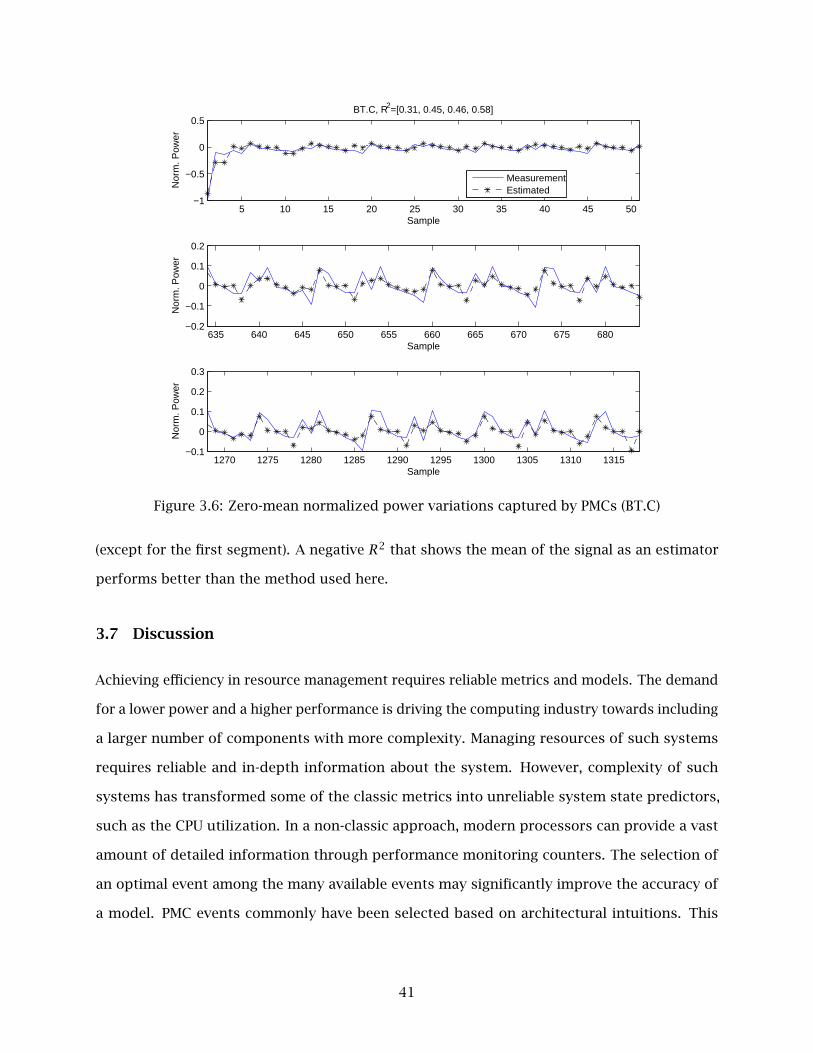
5 10 15 20 25 30 35 40 45 50−1
−0.5
0
0.5BT.C, R2=[0.31, 0.45, 0.46, 0.58]
Sample
Nor
m. P
ower
MeasurementEstimated
635 640 645 650 655 660 665 670 675 680−0.2
−0.1
0
0.1
0.2
Sample
Nor
m. P
ower
1270 1275 1280 1285 1290 1295 1300 1305 1310 1315−0.1
0
0.1
0.2
0.3
Sample
Nor
m. P
ower
Figure 3.6: Zero-mean normalized power variations captured by PMCs (BT.C)
(except for the first segment). A negative R2 that shows the mean of the signal as an estimator
performs better than the method used here.
3.7 Discussion
Achieving efficiency in resource management requires reliable metrics and models. The demand
for a lower power and a higher performance is driving the computing industry towards including
a larger number of components with more complexity. Managing resources of such systems
requires reliable and in-depth information about the system. However, complexity of such
systems has transformed some of the classic metrics into unreliable system state predictors,
such as the CPU utilization. In a non-classic approach, modern processors can provide a vast
amount of detailed information through performance monitoring counters. The selection of
an optimal event among the many available events may significantly improve the accuracy of
a model. PMC events commonly have been selected based on architectural intuitions. This
41

5 10 15 20 25 30 35 40 45 50−1
−0.5
0
0.5CG.C, R2=[0.94, 0.97, 0.97, 0.98]
Sample
Nor
m. P
ower
MeasurementEstimated
310 315 320 325 330 335 340 345 350 3550
0.02
0.04
0.06
Sample
Nor
m. P
ower
620 625 630 635 640 645 650 655 660 6650
0.02
0.04
0.06
Sample
Nor
m. P
ower
Figure 3.7: Zero-mean normalized power variations captured by PMCs (CG.C)
chapter proposes a systematic statistical method that efficiently finds the optimal PMC events
for a model.
In particular, this chapter studies single and multi-PMC selection methods for power-PMC
modeling purposes. We have provided application specific single-PMCs that are most correlated
with power for BT.C, CG.C, LU.C, and SP.C applications, as well as a unified group of PMCs for
all of our applications. Our proposed multi-PMC selection method provides the least redundant
PMC selection without facing obstacles faced by PCA-based methods, or their shortcoming in
accuracy. The best combination PMCs obtained through this method can produce estimates of
power with an R2 of 0.45-0.98 for our applications. In Chapter 4, we show that the time-domain
dependence of data in power-PMC trends can be used to build a more accurate model under
a fixed processor frequency. In Chapter 5, this model is extended to a variable frequency
environment.
42

5 10 15 20 25 30 35 40 45 50−1
−0.5
0
0.5LU.C, R2=[0.46, 0.67, 0.77, 0.8]
Sample
Nor
m. P
ower
MeasurementEstimated
1055 1060 1065 1070 1075 1080 1085 1090 1095 1100 1105−0.4
−0.2
0
0.2
0.4
Sample
Nor
m. P
ower
2110 2115 2120 2125 2130 2135 2140 2145 2150 2155 2160−0.4
−0.2
0
0.2
0.4
Sample
Nor
m. P
ower
Figure 3.8: Zero-mean normalized power variations captured by PMCs (LU.C)
5 10 15 20 25 30 35 40 45 50−1
−0.5
0
0.5SP.C, R2=[0.21, 0.29, 0.36, 0.45]
Sample
Nor
m. P
ower
MeasurementEstimated
1055 1060 1065 1070 1075 1080 1085 1090 1095 1100−0.2
−0.1
0
0.1
0.2
Sample
Nor
m. P
ower
2105 2110 2115 2120 2125 2130 2135 2140 2145 2150−0.2
0
0.2
0.4
0.6
Sample
Nor
m. P
ower
Figure 3.9: Zero-mean normalized power variations captured by PMCs (SP.C)
43

0 5 10 15 20 250
0.5
1BT.C, 64−Sample Segment R2
Segment
R2
1 2 3 4 5 6 7 8 9 10 11
−6−4−2
0
CG.C, 64−Sample Segment R2
Segment
R2
0 5 10 15 20 25 30 350
0.5
1LU.C, 64−Sample Segment R2
Segment
R2
0 5 10 15 20 25 30 350
0.5
1SP.C, 64−Sample Segment R2
Segment
R2
Figure 3.10: R2 for 64-sample segments
44

Chapter 4
Fixed Frequency Power Estimation
Power consumption and cooling issues are among the important design constraints of current
high-performance computing systems. Run-time power savings are mostly achieved by a power
management (PM) module, which dynamically optimizes the parameters of the system (e.g.,
processor voltage/frequency) to meet its performance and power requirements. Having access
to a real-time power measurement for an adaptive PM module is invaluable. Some of the recent
high-end servers provide embedded power and thermal measurements, such as HP[56] and IBM
PowerExecutive[64]. In most applications, variations in power consumption happen so quickly
that an external power measurement reading cannot provide an in time measurement for the
PM module. Applications suffering from power measurement delays, as well as systems without
an embedded measurement system, can significantly enjoy an accurate power estimation model.
An accurate power estimation model can perform as a control feedback loop for enhancing
decision making of the PM module. A delayed real power measurement (e.g., external) can be
used to update power estimation model in each step.
In Chapter 3, we have discussed an efficient method to choose appropriate PMCs for
power models and have provided the results for some of the NPB applications. This chapter
provides a model for estimating power consumption of a computing system using the current
and the past PMCs, as well as the past (non-intrusive) power measurements, under a fixed
processor frequency. The emergence of the computers have been revolutionary because of
their accurate operation in repetitive tasks, among other reasons and compared to a human
being’s abilities. This repetitive nature is seen in both hardware and software aspects of the
computing devices. In this chapter, we exploit this repetitiveness through the time dependence
between the measured metrics of a system to develop a power model. A linear model between
45

activity of the system (or its equivalent metrics, such as PMCs) and power consumption has
been considered by many previous work [15, 24, 25, 70, 88, 111]. In order to model the power
consumption of a system, we combine the time dependence of data within each metric signal
(i.e., power or PMC), in addition to the time dependence of data between the signals, with the
linear relationship between power consumption and PMCs. In particular, we use a multivariate
time-series approach to estimate the power consumption of the system. In order to obtain
an adaptive model that can adjust to the changes in a system, we combine the multivariate
time-series with a coefficient update algorithm. The proposed model is an autoregressive
moving average with exogenous inputs jointly used with a coefficient update algorithm [151]. A
change in frequency significantly affects the trends of power and PMC measurements. Therefore,
the discussion for variable frequency models is postponed to Chapter 5. This chapter studies
the efficiency of different update algorithms, such as recursive least squares, Kalman filter,
multivariate normal regression, and block multivariate normal regression. In addition, we study
the efficiency of simpler models (e.g., moving average) proposed by others [15, 53] for the
purpose of comparison with this work. The proposed method is both platform-independent
and application-independent, and does not require tapping into the system’s internal power
supply lines. This chapter studies the efficiency of power models from different aspects, such
as update algorithms, measurement delay, PMC selection, model parameters, and adaptation to
significant changes in the behavior of applications.
4.1 Related Work
Modeling the relationships of PMCs, workload, and power consumption of a system have
been approached from the architectural point of view previously [15, 24, 25, 70, 88, 111]. In
an orthogonal approach, we examine such relationships from a stochastic aspect. Although
similar time-series approaches have been used by researchers in other fields and applications
[27–29, 138, 147, 156], we propose using the ARMAX model [54] (described later in Section
4.2.1), as a promising candidate, for relating the power and performance metrics to each other.
The ARMAX model is capable of capturing the time dependence of the signals and the linear
relationship of power and PMC signals.
46
Many researchers have used PMCs or a sort of access rate metric in various energy
models of computer systems or some of its components [15, 25, 76, 111]. Contreras et al. [25]
estimate the power consumption of CPU and memory using a first-order linear sum of PMCs.
Joseph et al. [76] estimate the run-time power dissipation of different units of a Pentium Pro
processor using PMCs combined with architectural information provided by an architectural
processor power simulator. Rajamani et al. [111] have used PMCs to model instantaneous
performance and power of an Intel Pentium-M processor. Their approach is platform-specific
and needs training data set through micro-benchmarking. Some researchers [15] have found IPC
metrics useful in power estimation techniques. Bircher et al. [15] have used linear regression
models to estimate the power consumption of a single-core processor (Pentium 4). They report
that IPC related metrics show a strong correlation with CPU power, in particular the uops fetched
per cycle metric. A downside of many previous work is the necessity to tap the supply points
that power the processor to measure its power consumption.
Kalman filter [4] has been used in different ways to improve power or energy efficiency:
as a workload estimator [9], as well as a resource management tool [73]. Jain et al. [73] have
looked at stream resource management from a filtering point of view and have exploited KF
in their solution. Bang et al. [9] have proposed a KF-based workload estimation method for
dynamic voltage scaling, where they estimate the processing time of real-time multimedia
workloads. The way we use KF in this study is different from [9, 73] as we are not estimating
a workload or an unknown value. We use KF as a coefficient update algorithm for an ARMAX
model.
Time series prediction methods are well known and widely used in financial and indus-
trial problems, where ARMAX and autoregressive (AR) models are commonly utilized along with
system identification techniques. Some researchers have applied them to computing systems
[138, 147, 156]. Xu et al. [147] have studied predictive closed-loop control techniques for
systems management by comparing algorithms based on AR models, combined analysis of
variance (ANOVA) and AR models, and a multi-pulse model. Zhu et al. [156] as well as Wang et
al. [138] have discussed the strength of control theory approaches in computing systems, where
they use an ARMAX model along with system identification experiments to capture the dynamic
relationship between the CPU allocation to a web server and its measured mean response time.
47

To the best of our knowledge, an ARMAX model has not been used by others in modeling power
and performance relationships in computing systems.
Gurun et al. [53] have proposed a run-time feedback-based full system energy estimation
model for embedded devices, where a moving average of order zero (i.e., MA(0) model) of two
or three hardware and software performance counters is used to model communication or
computation energy consumption. The advantage of their approach is in using recursive least
squares linear regression with exponential decay for finding and updating the model parameters
on-the-fly. This work is substantially different than [53] as we are using an ARMAX model that
is non-zero order for both the AR part and the exogenous terms. The exogenous terms of our
model incorporates the past PMC values, while the autoregressive part of our model utilizes
feedback power measurement.
4.2 Models and Algorithms
In this section, we provide the mathematical background for the models and algorithms that
are used in this chapter.
4.2.1 ARMAX
Our estimation and prediction methodology in this thesis is based on autoregressive moving
average with exogenous inputs model [54]. ARMAX models are widely used in different fields,
such as in economic time-series prediction, hydrology, dendrochronology, etc. A general form
of ARMAX(p,q,b) represents a model with p autoregressive terms (i.e., AR(p)), q moving average
terms (i.e., MA(q)), and b exogenous inputs terms and is shown in (4.1). The Xi, c, εi, ψi, θi, ηi,
and di are scalar variables.
Xt = c + εt +p∑i=1
ψiXt−i +q∑i=1
θiεt−i +b∑i=1
ηidt−i (4.1)
where ψ1, · · · ,ψp and θ1, · · · ,θq are the parameters of the model, and η1, · · · ,ηb are the
parameters of the exogenous input.
48

We choose q = 0 in our ARMAX models and focus on p autoregressive terms and b
exogenous input terms. Therefore, our ARMAX(p, 0, b) model looks similar to an autoregressive
moving average model, ARMA(p,b). However, by definition, the exogenous input terms are not
related to the errors of previous modeling time steps. Thus, we do not use the term ARMA for
it. In order to estimate the parameters of our ARMAX models in this thesis we use different
algorithms, such as recursive least-squares filters and Kalman filters, in addition to standard
multivariate normal regressions.
4.2.2 Discrete-Time Kalman Filter
Kalman filter is a recursive filtering algorithm that enables us to estimate the state of a process
[4, 140]. It has been extensively studied and used in different fields of science and engineering.
The Kalman filter estimation is done in a way that the mean of the squared error is minimized.
The KF algorithm consists of a cycle of prediction and correction. In the prediction phase, the
process state in the upcoming time step is estimated. In the correction phase, based on the
observed measurement the algorithm is adjusted for a better prediction. The signal model
consists of a process equation shown in (4.2) and a measurement equation shown in (4.3).
xk+1 = Fkxk +wk (4.2)
zk = H′kxk + vk (4.3)
The state of process is shown by x ∈ Rn. The measurement of process is shown by
z ∈ Rm. The process noise is shown by the random variable wk with normal distribution N(0,Q).
The measurement noise is represented by the random variable vk with normal distribution
N(0,R). The initial process state x0 is N(x0,P0). The process noise wk, measurement noise
vk, and the initial process state x0 are jointly Gaussian and mutually independent. The n×n
matrix Fk relates the current state xk to the next state xk+1, when there is no process noise.
The m×n matrix H′k relates the current state xk to the current measurement zk. The matrix
H′k is the transpose of matrix Hk.
Here, we denote the a priori state estimate at time step k that uses all the measurements
up until time k−1 by xk/k−1. This quantity is defined as Exk | z0,z1, . . . ,zk−1 for k = 1,2,3, . . . .
49

The set of measurements up to time k− 1, which can be shown as z0,z1, . . . ,zk−1, is denoted
by Zk−1. We denote the a posteriori state estimate at time step k that uses the measurement zk
in addition to all the measurements up to time k− 1 as xk/k. In other words, xk/k is Exk | Zk.
The a priori and a posteriori estimate errors are defined as in (4.4) and (4.5).
ek/k−1 = xk − xk/k−1 (4.4)
ek/k = xk − xk/k (4.5)
The a priori and a posteriori error covariance matrices, Σk/k−1 and Σk/k, are calculated
using (4.6) and (4.7).
Σk/k−1 = E[xk − xk/k−1][xk − xk/k−1]′ | Zk−1 (4.6)
= Eek/k−1e′k/k−1
Σk/k = E[xk − xk/k][xk − xk/k]′ | Zk−1 (4.7)
= Eek/ke′k/k
In the Kalman filter equations the a posteriori state estimate xk/k is formulated as a
linear combination of an a priori estimate xk/k−1 and a weighted difference between an actual
measurement zk and a measurement prediction zk/k−1 as described in (4.8) and (4.9).
zk/k−1 = H′xk/k−1 (4.8)
xk/k = xk/k−1 +Kk(zk − zk/k−1) (4.9)
= xk/k−1 +Kk(zk −H′xk/k−1)
The zk − zk/k−1 part in (4.9) is called measurement innovation. The n ×m matrix Kk
in (4.9) is chosen to be the gain that minimizes the a posteriori error covariance Σk/k. For
conciseness, we skip the steps to derive a Kk (available in [140] and [4]). One form of Kk that
satisfies the aforementioned condition is shown in (4.12). The smaller Rk gets, the larger Kk
becomes. Therefore, the actual measurement zk is trusted more and its estimate zk/k−1 is
trusted less as the innovation factor – their difference (zk − zk/k−1) – will be compensated more
50

via a larger gain Kk. The smaller Σk/k−1 gets (as a result of a good estimation of x), the smaller
Kk becomes. Thus, the innovation factor will adjust the xk/k less away from the xk/k−1. The
prediction phase and correction phases of the Kalman filter can be summarized as below.
Prediction (Time Update)
In this phase of the Kalman filter, based on the information at time k, the process is projected
in time and xk+1/k and Σk+1/k at times k + 1 are estimated. The equations for updating the
Kalman filter in time are shown in (4.10) and (4.11).
xk+1/k = Fkxk/k (4.10)
Σk+1/k = FkΣk/kF′k +Qk (4.11)
Correction (Measurement Update)
Three major steps are done in measurement update phase. First, the Kalman gain Kk is updated
as in (4.12). Then based on the latest measurement zk an a posteriori state estimate xk/k is
generated using the equation (4.13). At last, an a posteriori error covariance estimate Σk/k is
calculated using (4.14).
Kk = Σk/k−1Hk(H′kΣk/k−1Hk + Rk)−1 (4.12)
xk/k = xk/k−1 +Kk(zk −H′xk/k−1) (4.13)
Σk/k = (I−KkH′k)Σk/k−1 (4.14)
After a time update and a measurement update step, these two phases are repeated and
at each cycle the current a posteriori variables will be the a priori variables in the next time
step.
4.2.3 Recursive Least-Squares Filter
The RLS algorithm is used for finding the coefficients of adaptive filters, and it recursively
produces the least squares of the error signal. Unlike many other adaptive filtering methods
51

that try to reduce the mean square error and require statistical information about the input
or the desired output signals, the RLS calculates a least squares error directly from the input
and the desired output. This makes the RLS filters a signal-dependent algorithm. The RLS filter
is computationally less intensive than the KF as it does not require any matrix inversion. It
is noteworthy to mention that a RLS filter can be reformulated as a KF as in (4.15) and (4.16).
Details can be found in [54].
xk+1 = λ−1/2xk (4.15)
zk = H′kxk + vk (4.16)
A summary of RLS algorithm [55] is presented in (4.17) to (4.22), where w(n) is the
tap-weight vector at time n, I is the identity matrix, λ is a small positive constant for high
signal-to-noise ratio (SNR), and is a large positive constant for low SNR. u(n) is the tap-input
vector at time n, λ−1 represents the exponential forgetting factor. P(n) is referred to as the
inverse correlation matrix and k(n) is referred to as the gain vector. The RLS algorithm in this
thesis uses λ = 0.9867.
w(0) = 0,P(0) = δ−1I (4.17)
π(n) = P(n− 1)u(n) (4.18)
k(n) = π(n)(λ+ u′(n)π(n))−1 (4.19)
ξ(n) = d(n)− w′(n− 1)u(n) (4.20)
w(n) = w(n− 1)+ k(n)ξ∗(n) (4.21)
P(n) = λ−1P(n− 1)− λ−1k(n)u′(n)P(n− 1) (4.22)
4.2.4 System Identification using KF
In this section, we explain how KF can be used for finding the coefficients of a scalar ARMA
equation. For the scalar ARMA equation presented in (4.23), the coefficients that we are
interested to find are a(1) , · · · , a(n+m). The system input measurements are represented by
52

uk and the system output measurements are denoted by yk, with a time subscript of k. In
a run-time model, the input and output values become available over time.
yk +n∑j=1
a(j)yk−j =m∑j=1
a(n+j)uk−j (4.23)
Let equation (4.23) describe the behavior of a system with constant coefficients a(i),
then with enough number of measurements and solving a set of linear equations one can
find those coefficients. However, if the coefficients are varying or the equation is not fully
modeling the system, in order to enable the model to follow the changes, the coefficients of the
ARMA equation should be adaptively updated as the new measurements become available. By
assuming that the coefficients in (4.23) are changing over time, we can rewrite the equation as
(4.24), where vk is a zero mean, white, Gaussian random process.
yk +n∑j=1
a(j)k yk−j =m∑j=1
a(n+j)k uk−j + vk (4.24)
We model the change of coefficients in (4.23) as if they are perturbed randomly over
time with an added noise. This change in coefficients can be written as in (4.25), where w(i)k
is a zero mean, white, Gaussian random process. The random processes w(i)k and w(j)
k
are independent for i ≠ j, also independent from vk in (4.24). For initialization purpose,
we assume each a(i)0 is a Gaussian random variable with an a priori mean and variance. The
variances of w(i)k and vk are also assigned according to the measurement values and the way
the a(i)k are varying.
a(i)k+1 = a(i)k +w
(i)k (4.25)
A Kalman filter approach, among others, can be used for finding and updating the
coefficients. For applying the Kalman filter on this identification problem, we define an (n+m)-
dimensional state vector xk as in (4.26). In addition, we use the w(j)k processes to define a
(n +m)-dimensional, white, zero mean, Gaussian vector process wk. Therefore, the state
53

equation can be written in a vector form as in (4.27) by using (4.25) and (4.26).
x(1)k = a(1)k , x(2)k = a(2)k , · · · , x(n+m)k = a(n+m)k (4.26)
xk+1 = xk +wk (4.27)
The Fk of the KF as defined in (4.2) is set as the identity matrix. The H′ matrix is defined
as a row vector in (4.28). The process zk is defined by zk = yk and using (4.24), (4.26), and
(4.28) we can formulate zk as in (4.29).
H′k = [−yk−1 · · · −yk−n uk−1 · · · uk−m] (4.28)
zk = H′kxk + vk (4.29)
One can notice the similarity of equations (4.27) and (4.29) with (4.2) and (4.3). At this
point, we have formulated the identification problem as a Kalman filter problem that we already
discussed its solution in section 4.2.2. The Kalman filter for this is shown in equations (4.30),
(4.31), and (4.32).
xk+1/k = [I−KkH′k]xk/k−1 +Kkzk (4.30)
Kk = Σk/k−1Hk[H′kΣk/k−1Hk + Rk]−1 (4.31)
Σk+1/k = Σk/k−1 −KkH′kΣk/k−1 +Qk (4.32)
In this solution, Rk = E[v2k] and Qk = E[wkw′k]. The initialization of equation (4.30)
is done by setting x0/−1 equal to the vector of a priori estimates of the coefficients. Equation
(4.32) is initialized with Σ0/−1 set equal to the a priori covariance matrix of the coefficients.
4.3 Experimental Framework
All the experiments in this chapter are conducted on the Dell PowerEdge R805 SMP server
and the Keithley power measurement setup that are specified in Section 3.2.1. Due to the
requirements of the libraries, applications, and the Linux kernels that are used to perform our
54

extensive tests, which this thesis includes a part of them, we have used two different software
setups. We have described the first configuration, CentOS software configuration, in Section
3.2.2. In the following, we explain the second software configuration of this work, Ubuntu
software configuration.
4.3.1 Ubuntu Software Setup
The second software configuration in this thesis, which we refer to as Ubuntu configuration, is
as follows. The operating system is Ubuntu Linux, running kernel version 2.6.28.9 patched with
the perfctr library version 2.6.39 for PMC measurement purposes. The measured PMC events
are: Dispatch stalls, memory controller page access event, retired x86 instructions, and cycles
with no FPU ops retired. These events are selected based on common architectural intuitions
for PMC-based power models. In Section 4.5.5, we also incorporate the optimal PMC selections
obtained in Chapter 3, for comparison with the above PMC events, using an ARMAX power-PMC
model.
A number of serial and OpenMP applications from the NAS parallel benchmarks [131]
suite are used in this study as benchmarks. These applications consists of NPB-3.3-SER bench-
mark suite (BT.A, BT.B, CG.B, EP.B, FT.B, LU.A, LU.B, SP.A, SP.B, UA.A, and UA.B) and NPB-3.3-OMP
(BT.C, CG.C, LU.B, SP.C, UA.B, and BT.B) running with eight threads. We have chosen those
applications in class B and C of NPB-3.3 that run for longer than 100 seconds on our system,
in order to have sufficient samples to compare the algorithms used in this study. In the serial
applications, we set the affinity of the application process to only one core.
4.4 Time-Series
In this section, we investigate the power consumption trend from a time-series perspective. In
Figure 4.1, we assess the degree of dependence in the data by showing the sample autocorre-
lation function (sample ACF) of differenced power consumption data. The horizontal lines in
this figure are the 95% confidence interval for Gaussian white noise process of length N , where
N is the sample length for each application. For a Gaussian white noise process it is expected
to have 95% of the ACF values (lags larger than zero) between the 95% bounds. We can see
55

0 10 20 30 40 50−0.5
0
0.5
1
Lag
Sa
mp
le A
uto
co
rre
latio
n
BT.C
0 10 20 30 40 50−0.5
0
0.5
1
Lag
Sa
mp
le A
uto
co
rre
latio
n
CG.C
0 10 20 30 40 50−1
−0.5
0
0.5
1
Lag
Sa
mp
le A
uto
co
rre
latio
n
LU.C
0 10 20 30 40 50−1
−0.5
0
0.5
1
Lag
Sa
mp
le A
uto
co
rre
latio
n
SP.C
Figure 4.1: Sample autocorrelation function of the differenced power trends
that power consumption signals for the studied benchmarks have many more than 5% ACF
values outside those bounds. This shows that there is a significant relationship in time between
our data samples. This strengthens the idea of using a time-series approach that includes an
autoregressive component for power modeling.
4.4.1 Power Estimation Model
In this section, we develop our power model that uses current PMC measurements, as well as
past power and PMC measurements, to estimate the current power consumption of the system
under a fixed processor frequency. This work utilizes a model and an update algorithm, depicted
in Figure 4.2. Two different models are used in this study: an autoregressive moving average
with exogenous inputs model and a zero-order moving average model. The ARMAX model is
our proposed method and the MA model (similar to [15, 53]) is for comparison purposes. The
ARMAX and MA models relate the input and output values to each other via different coefficients.
Finding and adaptively updating these coefficients can be done by different algorithms, such as
56

Figure 4.2: Block diagram of the model and coefficient update algorithm
RLS, KF, and MVNR. After each time step, the modeling error is provided to the coefficient update
algorithm and the coefficients are adjusted according to the objectives of the chosen algorithm.
For the MA model, two different update algorithms are used: recursive least squares that is
applied adaptively at each time step, as well as a multivariate normal regression that is applied
in advance to the whole trace. For the ARMAX model, four different update algorithms are used:
recursive least squares, Kalman filter, multivariate normal regression, and block multivariate
normal regression (BMVNR). The power estimations in this chapter are all performed offline in
MATLAB using collected real system measurements.
The first zero-order moving average model in this study is equipped with the RLS update
algorithm (similar to [53]), which is denoted as MA-0. The second zero-order MA model uses
a MVNR update algorithm. However, the MVNR algorithm is applied once to the entire signal
profile in advance. This is referred to as “Oracle” (similar to [15]). Oracle is a non-adaptive and
a non-causal algorithm and is merely implemented here for comparison purposes.
The MA-0 and Oracle models are defined in (4.33), where P[t] represents the power
measurement of the system at time t. There are jmax PMC events used in the model (for our
AMD Opteron jmax = 4). The jth PMC value (1 ≤ j ≤ jmax) at time t is shown as cj[t]. The
cj[t] is linearly related to the current power consumption measurement P[t] via a coefficient
αj . The values of αj are updated at each time step using a RLS algorithm for MA-0 and once
at the beginning for Oracle model using the whole trace. All the PMC measurements used in
this thesis (e.g., cj[t]) are normalized by the number of clock cycles of the sample, therefore,
57

representing a PMC rate.
P[t] =jmax∑j=1
αjcj[t] (4.33)
The ARMAX model used in this study is an ARMAX(n, 0, m + 1), which does not
include the moving average terms for non-exogenous inputs, provided in (4.34). The jth PMC
measurement at time t − i is denoted as cj[t − i], which is linearly related to the current power
consumption measurement P[t] via a coefficient αi,j . A past power measurement at time t − i,
P[t − i], is related to the current power measurement via a coefficient βi. The time window that
(4.34) covers includes the current and the previous m PMC measurements (m + 1 terms), as
well as the past n power measurements.
P[t] =m∑i=0
jmax∑j=1
αi,jcj[t − i]+n∑i=1
βiP[t − i] (4.34)
The values of αi,j and βi are updated at each time step using a coefficient update
algorithm (e.g., RLS, KF, MVNR, or BMVNR). The total number of these coefficients is jmax(m+
1)+n. ARMAX-RLS and ARMAX-KF models are formulated as explained in Section 4.2.4. For
ARMAX-MVNR models, the coefficients at time t = i are calculated using a multivariate normal
regression model that uses all the observed measurements from t = 0 until t = i. The ARMAX-
BMVNR model uses an algorithm similar to MVNR, however, at time t = i the coefficients are
calculated using the observations from t = i− T0 to t = i, where T0 is the length of the block.
The BMVNR algorithm has the advantage of having a fixed problem size to MVNR algorithm,
which has a growing number of calculations as time progresses.
4.5 Simulation Results of Real System Measurements
In this section, we provide different simulation results of the ARMAX model in estimating power
consumption from a real system measurement. In Section 4.5.1, we define the methodology we
use throughout this thesis for reporting modeling errors. Section 4.5.2 compares the efficiency
of different coefficient update algorithms in power estimation using an ARMAX model. Section
58

4.5.3 discusses the computational overhead of different coefficient update algorithms. Section
4.5.4 studies the sensitivity of the ARMAX model to the update delay of the measurements.
In Section 4.5.5, we investigate the effect of filter size and PMC event selection in estimation
efficiency of ARMAX-RLS models. Adaptation of ARMAX-RLS model to significant changes in
workload behavior is investigated in Section 4.5.6.
4.5.1 Error Reporting
In this work, we report the efficiency of the models by using coefficient of determination, R2,
mean absolute error of total signal (MAETS), and mean absolute error of dynamic signal (MAEDS).
Let xi be an observation and xi its estimated value for n readings (1 ≤ i ≤ n). Let x represent
the average of xi, x = 1n∑ni=1 xi. Let xmin and xmax be the minimum and maximum observed
values of xi. Our model efficiency metrics, R2, MAETS, and MAEDS are calculated as in (4.35),
(4.36), and (4.37), respectively.
R2 = 1−∑ni=1 (xi − xi)2∑ni=1 (xi − x)2
(4.35)
MAETS = 1n
n∑i=1
|xi − xi||xmax|
(4.36)
MAEDS = 1n
n∑i=1
|xi − xi|xmax − xmin
(4.37)
MAEDS uses the dynamic range of signal for calculating the error percentage, while
MAETS uses the maximum of signal. The maximum of signal, specially for power measurements,
contains a static part that never changes and may be significantly larger than the dynamic range
of the signal. Unfortunately, many related work report their error rates without removing the
static part of the estimated signals. When evaluating model errors, smaller denominator of
MAEDS in (4.37), xmax − xmin, makes it a more suitable metric than MAETS in (4.36) with a
larger denominator, |xmax|. For example, a 3% MAETS in estimation of a power consumption
signal with xmin = 280 and xmax = 310 might seem as a great result. However, it might not
seem so great when it is translated into its dynamic range as 280W of the signal never changes
and is related to idle power. For this example, the dynamic range of signal is xmax −xmin = 30
and therefore its MAEDS is 31% (10.3 times larger than its MAETS).
59

Some estimation methods tend to have a “training” or “warm-up” period to become
efficient, which its length depends also on parameters of the model. In this thesis, the whole
signal profile is used for the estimation phase. However, in order to avoid unfair comparisons,
the R2, MAEDS, and MAETS metrics are calculated using the measurements and their estimates
after the first hundred samples. In this thesis, we use the term “overall average of MAEDS
(or MAETS)” that is calculated in two steps: first, calculating the MAEDS (or MAETS) of each
benchmark, then calculating the average of the MAEDS (or MAETS) among all the benchmarks.
4.5.2 Coefficient Update Algorithms
In this section, we evaluate the effectiveness of the six models introduced in Section 4.4.1 for
different NPB benchmarks. We use the Ubuntu software configuration for this section to find a
suitable update algorithm for PMC-based power modeling. The model parameters used in this
section are: m = 4, n = 4, and jmax = 4 as defined in (4.33) and (4.34). The m and n ARMAX
parameters used in this thesis are chosen by manually searching for the values that do not
provide diminishing improvements. The PMC events used in this section are: dispatch stalls,
memory controller page access event, retired x86 instructions, and cycles with no FPU ops retired.
The block size for BMVNR is set arbitrarily to 75 samples in this study, based on the execution
length of our applications.
A part of the measured run-time power and its estimate for BT.C OpenMP application
running with eight threads is shown in Figure 4.3 for all the six model configurations. The
MAEDS of BT.C.OMP.8 shown in Figure 4.3 for RLS, MVNR, BMVNR, KF, MA-0, and Oracle methods
is 4.8%, 6.1%, 5.0%, 5.0%, 12.7%, and 14.9%, respectively. For most of the application traces,
RLS is the best method in terms of estimation error. The overall average of MAEDS for all the
applications studied in this work for RLS, MVNR, BMVNR, KF, MA-0, and Oracle methods is 8.0%,
8.1%, 8.2%, 8.5%, 15.6%, and 19.5%, respectively. Similarly, the overall average of MAETS among
all the applications for RLS, MVNR, BMVNR, KF, MA-0, and Oracle models is 0.62%, 0.67%, 0.70%,
0.68%, 1.26%, and 1.46%, respectively.
The MAEDS and MAETS metrics for all the applications in Ubuntu software configuration,
as well as the overall average, are presented in Figure 4.4. The minimum and maximum error
60

when using a MAEDS metric among all the applications are 3.4% and 41.5%, respectively. One can
notice the superior efficiency of ARMAX model when combined with RLS, for power estimation.
The order of the ARMAX model has an impact on the error levels and computation time. For
ARMAX models of a higher order than (4, 0, 4), given the PMC event selection used in this
section, we did not observe a significant improvement in power estimation efficiency. One can
conclude that ARMAX(4, 0, 4)-RLS is a good candidate for estimating power. Furthermore, no
lack of numerical robustness was observed from RLS algorithm in our modelings.
4.5.3 Computation-time Overhead
In order to have a real-time power estimation method integrated in a system, such as the ones
mentioned above, the estimation method requires to perform computation much faster than
the measurement sampling rate. An estimation method, such as MVNR, that uses an increasing
window size of inputs from the beginning until the estimation time, becomes slower over time,
and therefore not suitable for integration in a system. To alleviate this problem, one can use a
fixed-size block for MVNR (e.g., BMVNR) to lower the computational time of the MVNR method.
The KF method in principle should have a fixed computation size as it has only a fixed number
of matrix operations for each time step. However, depending on the parameters of the ARMAX,
the matrix inversion operations can be costly for the KF approach. In our simulation, the MVNR,
BMVNR, and KF methods ran 321, 37, and 117 times longer than the RLS method for BT.C.OMP-8
shown in Figure 4.3. The actual implementation of RLS takes approximately 710 microseconds
per sample on our experimental system.
4.5.4 Sensitivity to Measurement Update Delay
In this section, we investigate the impact of presence of a delay in receiving some of the
measurements in our ARMAX model (e.g., delay in receiving measurements from an external
digital multimeter). To include a lag time g between the current samples and the previous
samples, we rewrite the ARMAX equation of (4.34) as in (4.38), where ∆ij is defined as 1− δij ,
and δij is the Kronecker delta, which by definition its value is 1 for i = j; 0, otherwise. In other
words, ∆ij = 1 for i ≠ j; 0, otherwise.
61

250 260 270 280 290 300280
285
290
295
300
305
310
Sample
Pow
er (
W)
BT.C.OMP.8−threads − Power Estimation MAEDS = 4.8% MAETS = 0.6% g=0, m=4, n=4
MeasurementEstimated
(a) RLS
250 260 270 280 290 300280
285
290
295
300
305
310
Sample
Pow
er (
W)
BT.C.OMP.8−threads − Power Estimation MAEDS = 6.1% MAETS = 0.7% g=0, m=4, n=4
MeasurementEstimated
(b) MVNR
250 260 270 280 290 300280
285
290
295
300
305
310
Sample
Pow
er (
W)
BT.C.OMP.8−threads − Power Estimation MAEDS = 5.0% MAETS = 0.6% g=0, m=4, n=4 block=75
MeasurementEstimated
(c) BMVNR
250 260 270 280 290 300280
285
290
295
300
305
310
Sample
Pow
er (
W)
BT.C.OMP.8−threads − Power Estimation MAEDS = 5.0% MAETS = 0.6% g=0, m=4, n=4
MeasurementEstimated
(d) KF
250 260 270 280 290 300280
285
290
295
300
305
310
Sample
Pow
er (
W)
BT.C.OMP.8−threads − Power Estimation MAEDS = 12.7% MAETS = 1.5% g=0, m=0, n=0
MeasurementEstimated
(e) MA-0
250 260 270 280 290 300280
285
290
295
300
305
310
Sample
Pow
er (
W)
BT.C.OMP.8−threads − Power Estimation MAEDS = 14.9% MAETS = 1.8%
MeasurementEstimated
(f) Oracle
Figure 4.3: Comparing power estimation of BT.C running with 8 threads using RLS, MVNR,BMVNR, KF, MA-0, and Oracle models
62

RLS MVNR BMVNR KF MA-0 Oracle
45.0
RLS MVNR BMVNR KF MA-0 Oracle
35.0
40.0
45.0
RLS MVNR BMVNR KF MA-0 Oracle
30.0
35.0
40.0
45.0
MAEDS%
RLS MVNR BMVNR KF MA-0 Oracle
20.0
25.0
30.0
35.0
40.0
45.0
MAEDS%
RLS MVNR BMVNR KF MA-0 Oracle
15.0
20.0
25.0
30.0
35.0
40.0
45.0
MAEDS%
RLS MVNR BMVNR KF MA-0 Oracle
5.0
10.0
15.0
20.0
25.0
30.0
35.0
40.0
45.0
MAEDS%
RLS MVNR BMVNR KF MA-0 Oracle
0.0
5.0
10.0
15.0
20.0
25.0
30.0
35.0
40.0
45.0
MAEDS%
RLS MVNR BMVNR KF MA-0 Oracle
0.0
5.0
10.0
15.0
20.0
25.0
30.0
35.0
40.0
45.0
MAEDS%
RLS MVNR BMVNR KF MA-0 Oracle
0.0
5.0
10.0
15.0
20.0
25.0
30.0
35.0
40.0
45.0
MAEDS%
RLS MVNR BMVNR KF MA-0 Oracle
0.0
5.0
10.0
15.0
20.0
25.0
30.0
35.0
40.0
45.0
MAEDS%
RLS MVNR BMVNR KF MA-0 Oracle
0.0
5.0
10.0
15.0
20.0
25.0
30.0
35.0
40.0
45.0
MAEDS%
RLS MVNR BMVNR KF MA-0 Oracle
(a) MAEDS
RLS MVNR BMVNR KF MA-0 OracleRLS MVNR BMVNR KF MA-0 Oracle
3.5
4.0
RLS MVNR BMVNR KF MA-0 Oracle
3.0
3.5
4.0
RLS MVNR BMVNR KF MA-0 Oracle
2.5
3.0
3.5
4.0
MAETS%
RLS MVNR BMVNR KF MA-0 Oracle
1.5
2.0
2.5
3.0
3.5
4.0
MAETS%
RLS MVNR BMVNR KF MA-0 Oracle
1.0
1.5
2.0
2.5
3.0
3.5
4.0
MAETS%
RLS MVNR BMVNR KF MA-0 Oracle
0.5
1.0
1.5
2.0
2.5
3.0
3.5
4.0
MAETS%
RLS MVNR BMVNR KF MA-0 Oracle
0.0
0.5
1.0
1.5
2.0
2.5
3.0
3.5
4.0
MAETS%
RLS MVNR BMVNR KF MA-0 Oracle
0.0
0.5
1.0
1.5
2.0
2.5
3.0
3.5
4.0
MAETS%
RLS MVNR BMVNR KF MA-0 Oracle
0.0
0.5
1.0
1.5
2.0
2.5
3.0
3.5
4.0
MAETS%
RLS MVNR BMVNR KF MA-0 Oracle
0.0
0.5
1.0
1.5
2.0
2.5
3.0
3.5
4.0
MAETS%
RLS MVNR BMVNR KF MA-0 Oracle
0.0
0.5
1.0
1.5
2.0
2.5
3.0
3.5
4.0
MAETS%
RLS MVNR BMVNR KF MA-0 Oracle
0.0
0.5
1.0
1.5
2.0
2.5
3.0
3.5
4.0
MAETS%
RLS MVNR BMVNR KF MA-0 Oracle
(b) MAETS
Figure 4.4: MAEDS and MAETS of power estimation using different coefficient update algorithms
63

RLS MVNR KF
14
RLS MVNR KF
12
14
RLS MVNR KF
10
12
14
RLS MVNR KF
8
10
12
14
MA
ED
S%
RLS MVNR KF
6
8
10
12
14
MA
ED
S%
RLS MVNR KF
4
6
8
10
12
14
MA
ED
S%
RLS MVNR KF
2
4
6
8
10
12
14
MA
ED
S%
RLS MVNR KF
0
2
4
6
8
10
12
14
0 8 16 24 32 40 48 56
MA
ED
S%
RLS MVNR KF
0
2
4
6
8
10
12
14
0 8 16 24 32 40 48 56
MA
ED
S%
Gap (Samples)
RLS MVNR KF
0
2
4
6
8
10
12
14
0 8 16 24 32 40 48 56
MA
ED
S%
Gap (Samples)
RLS MVNR KF
0
2
4
6
8
10
12
14
0 8 16 24 32 40 48 56
MA
ED
S%
Gap (Samples)
RLS MVNR KF
Figure 4.5: The effect of delay on MAEDS using different coefficient update algorithms
P[t] =m∑i=0
jmax∑j=1
αi,jcj[t − i− g∆i0]+n∑i=1
βiP[t − i− g] (4.38)
In Figure 4.5 we present the impact of increasing the lag time from 0 to 56 samples,
with a step size of 8 samples, on overall MAEDS percentage of our applications. The increase
in overall MAEDS is under 4% for RLS, MVNR, and KF approaches, which shows an acceptable
delay tolerance of the ARMAX model.
4.5.5 PMC Selection and Filter Size
In this section we use the ARMAX-RLS model as our base model [151] to study the impact of
PMC event selection on power estimation efficiency. Furthermore, we study extreme cases of
model parameters (m and n) and their implication on estimation results. This section uses the
CentOS software configuration (detailed in Section 3.2.2).
We use two different sets of PMC events for each application to see their differences in
estimation performance. In our first selection, we use the top four correlated single PMCs for
each application from Tables 3.4, 3.5, 3.6, and 3.7, respectively for BT, CG, LU, and SP. We refer
to this selection of PMC as “Top PMCs”. In our second selection, we use the obtained results
from our proposed sub-space projection in Section 3.6.2. We refer to this selection of PMCs as
64
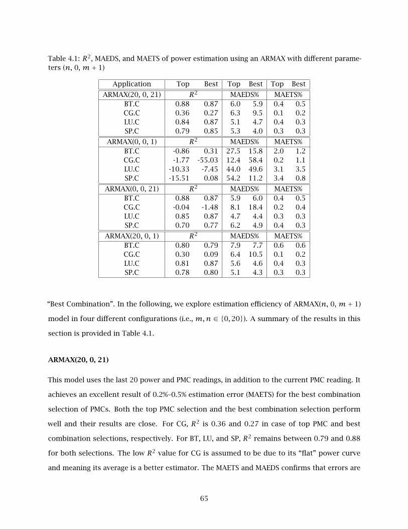
Table 4.1: R2, MAEDS, and MAETS of power estimation using an ARMAX with different parame-ters (n, 0, m+ 1)
Application Top Best Top Best Top Best
ARMAX(20, 0, 21) R2 MAEDS% MAETS%BT.C 0.88 0.87 6.0 5.9 0.4 0.5CG.C 0.36 0.27 6.3 9.5 0.1 0.2LU.C 0.84 0.87 5.1 4.7 0.4 0.3SP.C 0.79 0.85 5.3 4.0 0.3 0.3
ARMAX(0, 0, 1) R2 MAEDS% MAETS%BT.C -0.86 0.31 27.5 15.8 2.0 1.2CG.C -1.77 -55.03 12.4 58.4 0.2 1.1LU.C -10.33 -7.45 44.0 49.6 3.1 3.5SP.C -15.51 0.08 54.2 11.2 3.4 0.8
ARMAX(0, 0, 21) R2 MAEDS% MAETS%BT.C 0.88 0.87 5.9 6.0 0.4 0.5CG.C -0.04 -1.48 8.1 18.4 0.2 0.4LU.C 0.85 0.87 4.7 4.4 0.3 0.3SP.C 0.70 0.77 6.2 4.9 0.4 0.3
ARMAX(20, 0, 1) R2 MAEDS% MAETS%BT.C 0.80 0.79 7.9 7.7 0.6 0.6CG.C 0.30 0.09 6.4 10.5 0.1 0.2LU.C 0.81 0.87 5.6 4.6 0.4 0.3SP.C 0.78 0.80 5.1 4.3 0.3 0.3
“Best Combination”. In the following, we explore estimation efficiency of ARMAX(n, 0, m+ 1)
model in four different configurations (i.e., m,n ∈ 0,20). A summary of the results in this
section is provided in Table 4.1.
ARMAX(20, 0, 21)
This model uses the last 20 power and PMC readings, in addition to the current PMC reading. It
achieves an excellent result of 0.2%–0.5% estimation error (MAETS) for the best combination
selection of PMCs. Both the top PMC selection and the best combination selection perform
well and their results are close. For CG, R2 is 0.36 and 0.27 in case of top PMC and best
combination selections, respectively. For BT, LU, and SP, R2 remains between 0.79 and 0.88
for both selections. The low R2 value for CG is assumed to be due to its “flat” power curve
and meaning its average is a better estimator. The MAETS and MAEDS confirms that errors are
65

500 510 520 530 540 550295
300
305
310
315
320
Sample
Pow
er (
W)
BT.C − Power Estimation MAEDS = 5.9% MAETS = 0.5% R
2 = 0.87 , m=20, n=20
MeasurementEstimated
Figure 4.6: Power estimation of BT.C using ARMAX(20, 0, 21)
small for CG (MAEDS of 6.3% and 9.5%, and MAETS of 0.1% and 0.2%). We present some of the
observed and estimated power consumption of BT, CG, LU, and SP applications in Figure 4.6 ,
Figure 4.7, Figure 4.8, and Figure 4.9, respectively.
ARMAX(0, 0, 1) - No time dependence
This model uses only the current sample PMC measurements (no previous power/PMC) and is
equivalent of a MA-0 model. This is an extreme case for the purpose of comparison to other
scenarios and to understand estimation efficiency without looking at the past values. Except
for BT with the best combination selection of PMCs, the other applications for either selection
of PMCs do not provide a good R2. The dynamic range errors (MAEDS) for either selections
of PMCs are between 11% and 59%. It is important to notice, as a misleading measure, that
even with such a poor estimation performance, the total signal error average (MAETS) is in the
range of 0.2%–3.4% and 0.8%–3.5% for top PMCs selection and best combination PMC selection,
respectively.
66

500 510 520 530 540 550301
302
303
304
305
306
307
Sample
Pow
er (
W)
CG.C − Power Estimation MAEDS = 9.5% MAETS = 0.2% R
2 = 0.27 , m=20, n=20
MeasurementEstimated
Figure 4.7: Power estimation of CG.C using ARMAX(20, 0, 21)
500 510 520 530 540 550285
290
295
300
305
310
Sample
Pow
er (
W)
LU.C − Power Estimation MAEDS = 4.7% MAETS = 0.3% R
2 = 0.87 , m=20, n=20
MeasurementEstimated
Figure 4.8: Power estimation of LU.C using ARMAX(20, 0, 21)
67

500 510 520 530 540 550290
295
300
305
310
315
Sample
Pow
er (
W)
SP.C − Power Estimation MAEDS = 4.0% MAETS = 0.3% R
2 = 0.85 , m=20, n=20
MeasurementEstimated
Figure 4.9: Power estimation of SP.C using ARMAX(20, 0, 21)
ARMAX(0, 0, 21) - Exogenous inputs
This model uses the current and the past 20 PMC measurements and no previous power
measurement. Except for CG, the R2 measure shows a great estimation performance and its
performance is close to ARMAX(20, 0, 21) model. The dynamic range average estimation error
(MAEDS) range is 4.7%–8.1% and 4.4%–18.4% for the top PMC selection and best combination PMC
selection, respectively. The total signal average estimation error (MAETS) range is 0.2%–0.5%
overall for either PMC selections. Both MAETS and MAEDS metrics are close to the performance
metrics of ARMAX(20, 0, 21).
ARMAX(20, 0, 1) - Autoregressive model with current PMC
This model uses only the current PMC measurement and the past 20 power measurements. The
R2 metric performs very close to ARMAX(20, 0, 21) and ranges between 0.09–0.30 for CG and
0.78–0.87 for BT, CG, and LU. The difference in MAEDS metric between ARMAX(20, 0, 1) and
ARMAX(20, 0, 21) is less than 2.0% for all the applications/selections. Similarly, the difference
of MAETS metrics are less than 0.3%.
68

In short, using time dependence between power and/or PMC measurements significantly
improves the estimation efficiency. Furthermore, error calculations based on total power signal
can be misleading and hide model deficiencies, therefore we suggest using metrics such as
MAEDS.
4.5.6 Adapting to Significant Application Changes
Many HPC applications comprise of control structures that make their behavior repetitive for
some periods of their execution time (e.g., loops). Such repetitive behavior of an application
makes the task of estimation or prediction easier. Therefore, it is necessary to evaluate the
efficiency of an estimation or prediction model under extreme cases. For instance, a model can
be challenged by the periods of time that the behavior of the application varies significantly or
the system is in idle periods. For this purpose, we run multiple benchmarks (FT.B, SP.B, CG.C,
and LU.B) consecutively, with a sleep period (three seconds) between every two benchmarks. A
part of the power estimation of ARMAX-RLS and its error for this test case is shown in Figure
4.10. This test uses the Ubuntu software configuration (see Section 4.3.1 for the PMC events
used). This allows us to just focus on the extreme part of the trace. One can notice that the
estimation error increases as soon as the CG.C benchmark ends. However, the model feedback
adjusts the increase in error to follow the power trend more accurately. Although during the
idle period the activity of the system is minimal and the PMCs are not changing significantly,
the power estimation follows the power measurements. When the next application starts (i.e.,
LU.B), the PMCs are suddenly changed and the estimates follow the new power trend.
The overshoot or undershoot in power estimation varies based on the “experience” of
the coefficient update algorithm through the different parts of a trace. The RLS algorithm, and
some other algorithms, are data dependent. The update algorithm changes the coefficients
significantly if a significant error is observed and each chosen set of the coefficients almost
result in a unique behavior of the estimator. The presented extreme case result in Figure 4.10 is
an example scenario, keeping in mind that other traces result in different worst case estimation
errors (larger or smaller errors).
69

900 910 920 930 940 950 960 970100
150
200
250
300
350
Sample
Power (W)
Multi-Application - Power Estimation MAEDS = 1.7% MAETS = 0.7% g=0, m=4, n=4
Measurement
Estimated
900 910 920 930 940 950 960 9700
10
20
30
40
50
Sample
Error (W)
cg.C ends
lu.B starts
Idleperiod
Figure 4.10: Run-time power estimation of multiple applications (extreme cases: idle period,and start/end of a benchmark)
4.6 Discussion
This chapter studies efficiency of our multivariate time-series based power model from different
aspects. We have conducted our experiments on a real multi-core system, and gathered PMC
values and system power consumption measurements in real-time when running serial and
OpenMP applications from the NAS Parallel Benchmark suite. We have compared the efficiency
of different coefficient update algorithms, such as KF, RLS, MVNR, and BMVNR, in power
estimation using an ARMAX model. The overall average of MAETS among all the applications
for RLS, MVNR, BMVNR, and KF models is 0.62%, 0.67%, 0.70%, and 0.68%, respectively. The RLS
algorithm performs the best among the studied algorithm and has one of the least computational
overheads. The ARMAX model combined with RLS, MVNR, and KF algorithms perform with a
70

small sensitivity to measurement update delay (less than 4% increase in MAEDS for up to 56
time sample delays). This is desirable in systems with a long delay between external system
measurements and model update. We have found that larger filter sizes can improve the
estimation efficiency. In fact, as long as the time dependence of the inputs or outputs of the
system is captured in the ARMAX model (i.e., m > 1 or n > 1 in an ARMAX(n, 0, m+ 1) model),
a better estimation efficiency is observed. We have also shown that an optimal PMC selection for
power modeling can improve the efficiency of the estimation model. However, the improvement
gained through the time dependence aspect is more significant than the PMC selection. We have
presented that an adaptive multivariate time-series model such as the ARMAX-RLS can follow
the significant changes in the workload behavior.
In summary, we have shown that ARMAX-RLS is a great candidate for power modeling
using PMCs, under a fixed processor frequency. In Chapter 5, we propose a method to use
the ARMAX-RLS model for a variable frequency environment [150]. Later in Chapter 6, the
ARMAX-RLS model obtained in this chapter is used to develop a run-time power and PMC
prediction system [154].
71

Chapter 5
Variable Frequency Power Estimation
In Chapter 3, we presented a methodology to efficiently choose performance monitoring
counters for modeling power consumption of a system. Chapter 4 studied application of
ARMAX models combined with coefficient update algorithms, such as RLS, for estimating
system power consumption using PMCs under a fixed processor frequency. Any change in the
operating frequency of a processor impacts its power consumption and performance monitoring
counters. In most cases, the changes of such metrics do not follow the changes of frequency
linearly. Therefore, it is not straightforward to use the changing metrics of the system in
a time-series model despite knowing the exact value of frequency. Many prior attempts by
researchers [47, 83, 123] have used a regression based approach which tries to capture the
impact of frequency scaling in system metrics by differentiating between scaling and non-scaling
metrics. These methods suffer from a limited set of PMCs that fit the theoretical model, which
mostly represents an oversimplified version of a real system or workload. This chapter provides
a novel solution to this problem.
Our approach is based on a practical Gaussian approximation [150]. Using the Gaussian
distribution properties, we use the mean and variance of the obtained signals under different
frequency settings to scale and offset them into a unified trend. We choose a unified trend with
a zero mean and unit variance. Our approach is adaptive and does not dictate the usage of any
specific PMC event.
5.1 Related Work
Zhang et al. [155] have described an on-line regression-based power estimation and model
generation framework for smart-phones. Their approach uses the built-in battery voltage
72

sensors in smart-phones. In their regression model, they use the CPU utilization and the
frequency-voltage settings to capture the frequency-power relationship. Gandhi et al. [46] find
that the power-to-frequency curve for both clock throttling and DVFS can be approximated as a
linear function. They find for the combination of clock throttling and DVFS, power-to-frequency
relationship exhibits a piecewise linear characteristic. They approximate this relationship using
a cubic fit.
Rountree et al. [113, 114] have proposed using a new architectural PMC event, leading
loads, to model the relationship between CPU clock frequency, memory usage, and performance.
Through simulations, they have observed improvements in the efficiency of frequency scaling
models. Most available models divide the program execution into CPU time, which scales with
frequency scaling, and bus time, which does not scale with frequency scaling [113]. Snowdon et
al. [123] have proposed a general regression-based PMC model for the prediction of power and
energy under DVFS. Lee et al. [83] have proposed a model to predict the performance impact of
DVFS. They have used a first-order linear regression analysis to estimate performance impact
from monitored activity information such as cycles per instruction (CPI) and the number of
memory accesses. Ge et al. [47] use on-chip and off-chip time to provide a speedup model that
accounts for the degree of parallelism and the effects DVFS. Sasaki et al. [119] have used a
PMC-based regression approach to model the scaling of performance through DVFS.
Our work in this thesis is different from the aforementioned work: we provide an
adaptive solution that does not require a prior model calibration. Given the small and limited
number of available PMC registers, our approach does not dictate the type of PMC events that
should be monitored in order to be able to predict the scaling impact of DVFS. We exploit the
probability distribution properties of power and PMC signals to provide a simple and effective
solution for prediction of scaling impact of DVFS on power and PMC signals.
5.2 Effect of Variable Frequency on PMC and Power Trends
Changing frequency of a processor scales its processing speed and power consumption. How-
ever, this does not directly scale the performance, power consumption, or the operating
frequency (if exists) of other modules in the system, such as memory modules, storage devices,
73

1500 1550 1600 1650 1700200
250
300
350Power
Wat
ts
1500 1550 1600 1650 1700
1000
1500
2000
Frequency
MH
z
1500 1550 1600 1650 17000
0.2
0.4
0.6
0.8Microarchitectural Early Cancel of an Access (Rate)
Eve
nt/C
ycle
Sample
1500 1550 1600 1650 17000
0.05
0.1
0.15
0.2Data Cache Lines Evicted (Rate)
Eve
nt/C
ycle
1500 1550 1600 1650 17000.1
0.15
0.2L2 Fill/Writeback (Rate)
Eve
nt/C
ycle
1500 1550 1600 1650 17000
5
10
15Retired MMX/FP Instructions (Rate)
Eve
nt/C
ycle
Sample
Figure 5.1: The impact of frequency changes on power consumption and PMCs of BT.C
and interconnection networks. Due to the scaled performance of processor and its scaled
number of requests for other modules, some of the other modules might experience a scaled
load. The overall performance and power consumption of an application depends on the usage
of each module. Therefore, overall performance and power consumption varies among different
applications when processor frequency is scaled.
This unknown scaling, to some extent, is also applicable to PMCs. As an example, Figure
5.1 shows the processor frequency, power consumption, and four PMC events of the system
while running BT.C application on CentOS software configuration (detailed in Section 3.2.2).
It is noticeable that the change in frequency leads to sudden changes in the signal level, its
pattern, and its statistics (e.g., mean and variance). The signal scaling varies among different
events and applications.
74

In addition, different phases of an application or different applications tend to have
different activity levels for each PMC. This means that their mean and variance is varying over
time. For illustration of this effect, we have consecutively run five NPB-OMP applications. These
applications are BT.C, LU.C, SP.C, FT.C, and MG.C running with eight threads while changing
the frequency of all eight cores simultaneously according to a previously generated random
frequency pattern (duration and value). In this thesis, we choose an identical frequency for all
the cores in the system to avoid a possible load imbalance. Figure 5.2 shows the frequency,
instantaneous value of power consumption, as well as its mean and variance associated with
each frequency, calculated based on the history of the signal up to each point in time. Similarly,
Figure 5.3, Figure 5.4, Figure 5.5, and Figure 5.6 show the measured PMC rates, as well as their
mean and variance up to each time sample.
It is noticeable that the mean and variance of power consumption signal over different
applications do not vary significantly compared to the PMC signals, after accumulating enough
samples. However, the range, pattern, mean, and variance of the PMC signals can vary signifi-
cantly over time for different applications and their different phases. For Micro-architectural
Early Cancel of an Access, from sample 4000 to the end of samples, there is a significant change
in the pattern of the PMC rate as the applications show different behaviors. For Data Cache
Lines Evicted, for samples 1500–4500 and 6000–7000 a significant change of pattern can be
noticed. For L2 Fill/Writeback, samples of 6000–7000 exhibit a significant different pattern to
the rest of the signal. For Retired MMX/FP Instructions, up to five distinct phases can be seen in
the signal pattern and its statistics.
The ARMAX model used in this thesis performs the best when its signals are station-
ary. Therefore, the changes of signal statistics due to variations of frequency or variations of
application behavior is not desired for an ARMAX model. The ARMAX-RLS model is contin-
uously adjusting itself to changes of application behavior. However, in a variable frequency
environment, if the signals are applied to an ARMAX as they are measured, their significant
changes that are the result of frequency difference will be continuously adjusted by changing
the obtained model (i.e., ARMAX coefficients). This can result in an unreliable modeling. The
rest of this chapter focuses on addressing this issue and providing a method to accurately use
the ARMAX-RLS methods in a variable frequency environment.
75

010
0020
0030
0040
0050
0060
0070
0020
0
300
400
Power (Watts)
BT
, LU
, SP
, FT
, and
MG
(C
lass
C)
− P
ower
010
0020
0030
0040
0050
0060
0070
00
1000
1500
2000
Frequency (MHz)
010
0020
0030
0040
0050
0060
0070
000
0.2
0.4
Mean
1.0
GH
z1.
2 G
Hz
1.4
GH
z1.
7 G
Hz
2.0
GH
z
010
0020
0030
0040
0050
0060
0070
00024
x 10
−4
Sam
ple
Variance
1.
0 G
Hz
1.2
GH
z1.
4 G
Hz
1.7
GH
z2.
0 G
Hz
Figu
re5.2
:V
aria
ble
freq
uen
cyp
ow
erco
nsu
mp
tion
of
con
secu
tive
exec
uti
on
of
BT
.C,L
U.C
,SP.C
,FT
.C,a
nd
MG
.C
76

010
0020
0030
0040
0050
0060
0070
000510
x 10
8
PMC Rate
BT
, LU
, SP
, FT
, and
MG
(C
lass
C)
− M
icro
arch
itect
ural
Ear
ly C
ance
l of a
n A
cces
s (R
ate)
010
0020
0030
0040
0050
0060
0070
00
1000
1500
2000
Frequency (MHz)
010
0020
0030
0040
0050
0060
0070
000
0.51
Mean
1.
0 G
Hz
1.2
GH
z1.
4 G
Hz
1.7
GH
z2.
0 G
Hz
010
0020
0030
0040
0050
0060
0070
000
0.050.
1
Sam
ple
Variance
1.
0 G
Hz
1.2
GH
z1.
4 G
Hz
1.7
GH
z2.
0 G
Hz
Figu
re5
.3:
Var
iab
lefr
equ
ency
Mic
ro-a
rch
itec
tura
lEa
rly
Can
cel
of
anA
cces
s(r
ate)
of
con
secu
tive
exec
uti
on
of
BT
.C,L
U.C
,SP.
C,F
T.C
,an
dM
G.C
77

010
0020
0030
0040
0050
0060
0070
000510
x 10
7
PMC Rate
BT
, LU
, SP
, FT
, and
MG
(C
lass
C)
− D
ata
Cac
he L
ines
Evi
cted
(R
ate)
010
0020
0030
0040
0050
0060
0070
00
1000
1500
2000
Frequency (MHz)
010
0020
0030
0040
0050
0060
0070
000
0.050.
1
Mean
1.
0 G
Hz
1.2
GH
z1.
4 G
Hz
1.7
GH
z2.
0 G
Hz
010
0020
0030
0040
0050
0060
0070
00024
x 10
−3
Sam
ple
Variance
1.
0 G
Hz
1.2
GH
z1.
4 G
Hz
1.7
GH
z2.
0 G
Hz
Figu
re5.4
:V
aria
ble
freq
uen
cyD
ata
Cac
he
Lin
esEv
icte
d(r
ate)
of
con
secu
tive
exec
uti
on
of
BT
.C,L
U.C
,SP.C
,FT
.C,a
nd
MG
.C
78

010
0020
0030
0040
0050
0060
0070
00024
x 10
8
PMC Rate
BT
, LU
, SP
, FT
, and
MG
(C
lass
C)
− L
2 F
ill/W
riteb
ack
(Rat
e)
010
0020
0030
0040
0050
0060
0070
00
1000
1500
2000
Frequency (MHz)
010
0020
0030
0040
0050
0060
0070
000
0.1
0.2
Mean
1.0
GH
z1.
2 G
Hz
1.4
GH
z1.
7 G
Hz
2.0
GH
z
010
0020
0030
0040
0050
0060
0070
000
0.00
5
0.01
Sam
ple
Variance
1.
0 G
Hz
1.2
GH
z1.
4 G
Hz
1.7
GH
z2.
0 G
Hz
Figu
re5.5
:V
aria
ble
freq
uen
cyL2
Fill
/Wri
teb
ack
(rat
e)of
con
secu
tive
exec
uti
on
of
BT
.C,L
U.C
,SP.C
,FT
.C,a
nd
MG
.C
79

010
0020
0030
0040
0050
0060
0070
000510
x 10
9
PMC Rate
BT
, LU
, SP
, FT
, and
MG
(C
lass
C)
− R
etire
d M
MX
/FP
Inst
ruct
ions
(R
ate)
010
0020
0030
0040
0050
0060
0070
00
1000
1500
2000
Frequency (MHz)
010
0020
0030
0040
0050
0060
0070
000510
Mean
1.
0 G
Hz
1.2
GH
z1.
4 G
Hz
1.7
GH
z2.
0 G
Hz
010
0020
0030
0040
0050
0060
0070
0001020
Sam
ple
Variance
1.
0 G
Hz
1.2
GH
z1.
4 G
Hz
1.7
GH
z2.
0 G
Hz
Figu
re5.6
:V
aria
ble
freq
uen
cyR
etir
edM
MX
/FP
Inst
ruct
ion
s(r
ate)
of
con
secu
tive
exec
uti
on
of
BT
.C,L
U.C
,SP.C
,FT
.C,a
nd
MG
.C
80

5.3 Zero Mean Unit Variance Module
The trend of power consumption or a PMC event is not necessarily a Gaussian or stationary
time-series. The goal in this chapter is to overcome the impact of change of frequency on
time-series models. The proposed solution for this problem is based on a practical Gaussian
approximation. Assuming that the input signals are Gaussian enables us to use the Gaussian
distribution properties for simplifying our approach. In particular, the first two moments of a
Gaussian distribution (mean and variance) are sufficient to completely describe it. Therefore,
for statistical convenience, we assume that our power and PMC trends are Gaussian.
Furthermore, we assume that the input signals to the time-series are weakly stationary
for a fixed frequency setting. Under frequency scaling, we attempt to transform the measured
signal to a signal that is weakly stationary. Given the Gaussian approximation, this translates
into keeping the mean and variance of the input signals identical and consistent under different
frequency settings. For each processor frequency, mean and variance of the input signals are
different and varies over time. To obtain a weakly stationary signal for each of the input signals,
we use a zero mean and unit variance transformation. The ZMUV transformation makes sure
that the mean and variance of the different segments of the signal, which are associated with
different frequency settings, are identical.
Let S be a power or PMC signal of the system, with a total of n samples, over the
execution time of an application. Let f(t) = fi represent the frequency of the processor at
the time sample t. Assume that processor can have p different frequencies, fi ∈ f1, · · · , fp,
ordered from the smallest frequency f1 to the largest frequency fp (p = 5 for this study). Signal
S can be split based on the frequency of each time sample into p smaller signals Sf1 , · · · ,Sfp
that each only contain the samples of time associated with one of the available frequencies. One
way of obtaining this signal is: for each frequency fi (i = 1, · · · , p), initialize u = 1 and iterate
t over time (t = 1, · · · , n), if f(t) = fi then Sfi(u) = S(t) and u = u+ 1. The total number of
measurement points does not change in this method as shown in (5.1).
|S| =p∑i=1
|Sfi| (5.1)
81

Model Error & Measurements
Coefficients
Model (ARMAX, MA, etc.)
Coefficient Update (RLS, KF, MVNR, etc.)
Scale and Offset Power, PMC
ZMUV Measured Signals
Estimation or Prediction of ZMUV Signals
Estimation or Prediction
Inverse
Inverse Scale and
Offset
Zero Mean Unit Variance
Figure 5.7: Block diagram of model, coefficient update and scaling (zero mean unit variance)modules
In order to be able to adjust the mean and variance of the power and PMC signals
associated with different frequencies into a unified Gaussian time-series that can be used in an
ARMAX-RLS model, we keep track of their mean, µfi , and variance, σ2fi . Then, before the power
and PMC trends are provided to the ARMAX-RLS model, we scale and offset the trend to a zero
mean and unit variance trend for each trend associated with a frequency. This enables us to
adapt different segments of power and PMC trends that are associated with different processor
frequencies to a unified zero mean and unit variance time-series model (e.g., ARMAX-RLS). After
model calculations and estimation, the unified signal can be translated from the unified ZMUV
to a specific frequency by using the inverse scale and offset associated with the target frequency.
A block diagram of modeling module, coefficient update module, and ZMUV module is shown
in Figure 5.7.
5.3.1 Scale and Offset
Let Sfi show a measured signal associated to frequency fi. Assume Sfi has a Gaussian distri-
bution with mean µfi and variance of σ2fi . We use the transformation in (5.2) to obtain a zero
82

mean and unit variance Gaussian distribution.
ufi =Sfi − µfiσfi
(5.2)
The inverse of the above transformation (5.3) is used to translate ZMUV signals into
signals associated to their frequency.
Sfi = ufiσfi + µfi (5.3)
For a real-time signal such as Sfi , mean and variance values are not known a priori and
vary over time. Therefore, we define the mean and variance of these metrics as a time dependent
variable with mean µfi(t) and variance σ2fi(t). The ZMUV module has the responsibility of
keeping track of mean µfi(t) and variance σ2fi(t) for all the signals. As an example, the unified
ZMUV signals power consumption and one of the PMCs of FT.C, along with their mean and
variance over time, are shown in Figure 5.8, and Figure 5.9. A cumulative mean and variance
is used in this thesis, however, for applications with a significantly long execution time it is
recommended that a running mean and variance to be used. Using a running mean and variance
makes these metrics more adaptive when the number of observations are significantly large.
5.4 ZMUV Signal Estimation Results
In this section, we present the results of power estimation of a zero mean unit variance signal
obtained from scaled and offset values from different frequencies. Figure 5.10 depicts both the
ZMUV power signal and its estimate for a part of the execution of BT.C execution. Table 5.1
summarizes the R2 and MAEDS of estimation of ZMUV power signals for BT.C, LU.C, SP.C, FT.C,
and MG.C for ARMAX(4, 0, 5) and ARMAX(10, 0, 11) models. Both models perform similarly,
however, it is noticed that the model with the shorter windows, ARMAX(4, 0 , 5), slightly
performs better. As the signals in this estimation has a zero mean their MAEDS and MAETS
values are identical.
83

0 50 100 150 200 250 300 350 400−5
0
5
ZM
UV
Pow
er
FT.C − Power
0 50 100 150 200 250 300 350 400
1000
1500
2000
Fre
quen
cy (
MH
z)
0 50 100 150 200 250 300 350 4000
0.1
0.2
0.3
0.4
Mea
n
1000 MHz 1200 MHz 1400 MHz 1700 MHz 2000 MHz
0 50 100 150 200 250 300 350 4000
0.5
1
1.5x 10
−3
Sample
Var
ianc
e
1000 MHz 1200 MHz 1400 MHz 1700 MHz 2000 MHz
Figure 5.8: ZMUV signal, mean, and variance of power consumption for FT.C
Table 5.1: R2 and MAEDS of variable frequency ZMUV power estimation using ARMAX(4, 0, 5)and ARMAX(10, 0, 11)
ARMAX (4, 0, 5) (10, 0, 11) (4, 0, 5) (10, 0, 11)Application R2 R2 MAEDS% MAEDS%
BT.C 0.83 0.82 7.31 7.74LU.C 0.79 0.78 8.24 8.50SP.C 0.81 0.80 7.97 8.28FT.C 0.44 0.38 10.73 11.31MG.C 0.45 0.37 12.02 13.57
5.5 Power Estimation Results
In this section, we provide the power estimation results for BT.C, LU.C, SP.C, FT.C, and MG.C
after inverse transformation from the ZMUV signals. The ARMAX(4, 0, 5) is chosen for these
results. In a variable frequency environment, power consumption of all applications in this
chapter are estimated with a MAEDS of less than 10%, a MAETS of less than 2.7%, and an R2 of
larger than 0.74. Table 5.2 summarizes the statistics of power estimation for this section. A
84

0 50 100 150 200 250 300 350 400−5
0
5
PM
C R
ate
FT.C − Microarchitectural Early Cancel of an Access (Rate)
0 50 100 150 200 250 300 350 400
1000
1500
2000
Fre
quen
cy (
MH
z)
0 50 100 150 200 250 300 350 4000
0.2
0.4
0.6
0.8
Mea
n
1000 MHz 1200 MHz 1400 MHz 1700 MHz 2000 MHz
0 50 100 150 200 250 300 350 4000
0.02
0.04
0.06
0.08
Sample
Var
ianc
e
1000 MHz 1200 MHz 1400 MHz 1700 MHz 2000 MHz
Figure 5.9: ZMUV signal, mean, and variance of Micro-architectural Early Cancel of an Access(rate) for FT.C
Table 5.2: R2, MAEDS, and MAETS of variable frequency power estimation using ARMAX(4, 0, 5)Application R2 MAEDS% MAETS%
BT.C 0.94 5.32 1.60LU.C 0.91 5.83 1.63SP.C 0.92 5.38 1.30FT.C 0.82 9.53 2.60MG.C 0.75 8.05 2.05
part of the power consumption and its estimate under a random length and value of frequency
for BT.C, LU.C, SP.C, FT.C, and MG.C are shown in Figure 5.10, Figure 5.11, Figure 5.12, Figure
5.13, and Figure 5.14, respectively.
85

1400 1420 1440 1460 1480 1500 1520 1540 1560 1580 1600−5
0
5
Sample
ZM
UV
Pow
er
BT.C − M=4, N=4, MLag=0, NLag=0, (100..End): MAETS=7.31%, MAEDS=7.31%, R2 = 0.83
1400 1420 1440 1460 1480 1500 1520 1540 1560 1580 1600
1000
1500
2000
Fre
quen
cy (
MH
z)
MeasuredEstimatedFrequency
1400 1420 1440 1460 1480 1500 1520 1540 1560 1580 1600200
300
400
Sample
Pow
er (
Wat
ts)
BT.C − M=4, N=4, MLag=0, NLag=0, (100..End): MAETS=1.68%, MAEDS=5.57%, R2 = 0.93
1400 1420 1440 1460 1480 1500 1520 1540 1560 1580 1600
1000
1500
2000
Fre
quen
cy (
MH
z)
MeasuredEstimatedFrequency
Figure 5.10: Estimation of the ZMUV power signal and its equivalent in original frequencies forBT.C
86

2200 2220 2240 2260 2280 2300 2320 2340 2360 2380 2400200
300
400
Sample
Pow
er
(Watts)
LU.C − M=4, N=4, MLag=0, NLag=0, (100..End): MAETS=1.63%, MAEDS=5.83%, R2 = 0.91
2200 2220 2240 2260 2280 2300 2320 2340 2360 2380 2400
1000
1500
2000
Fre
quency (
MH
z)
Measured
Estimated
Frequency
Figure 5.11: Variable frequency power estimation of LU.C
2000 2020 2040 2060 2080 2100 2120 2140 2160 2180 2200230
240
250
260
270
280
290
300
310
320
330
Sample
Pow
er
(Watts)
SP.C − M=4, N=4, MLag=0, NLag=0, (100..End): MAETS=1.30%, MAEDS=5.38%, R2 = 0.92
2000 2020 2040 2060 2080 2100 2120 2140 2160 2180 2200
1000
1100
1200
1300
1400
1500
1600
1700
1800
1900
2000
Fre
quency (
MH
z)
Measured
Estimated
Frequency
Figure 5.12: Variable frequency power estimation of SP.C
87

100 120 140 160 180 200 220 240 260 280 300200
300
400
Sample
Pow
er
(Watts)
FT.C − M=4, N=4, MLag=0, NLag=0, (100..End): MAETS=2.60%, MAEDS=9.53%, R2 = 0.82
100 120 140 160 180 200 220 240 260 280 300
1000
1500
2000
Fre
quency (
MH
z)
Measured
Estimated
Frequency
Figure 5.13: Variable frequency power estimation of FT.C
100 110 120 130 140 150 160 170 180 190 200200
300
400
Sample
Pow
er
(Watts)
MG.C − M=4, N=4, MLag=0, NLag=0, (100..End): MAETS=2.05%, MAEDS=8.05%, R2 = 0.75
100 110 120 130 140 150 160 170 180 190 200
1000
1500
2000
Fre
quency (
MH
z)
Measured
Estimated
Frequency
Figure 5.14: Variable frequency power estimation of MG.C
88

5.6 Discussion
This chapter provided a solution to variable frequency power estimation using a multivariate
time-series method, such as ARMAX-RLS. The key to this solution is to scale and offset the
signals for different frequencies in a way that will maintain equal means and variances. The
zero mean unit variance module in this chapter performs this equalization of signal statistics
transparently before providing the signals to ARMAX-RLS layer. The inverse signal translation
is performed after obtaining the estimated values.
The results in this chapter show that the time dependence of signals can provide an
accurate model even when frequency of the processors are changing. In Chapter 6, we exploit
the time dependence to a larger extent and study the efficacy of prediction of power and PMC
signals using the proposed ARMAX-RLS equipped with a ZMUV module.
89

Chapter 6
Power and Performance Prediction
Accurate prediction of power and performance metrics can be leveraged into valuable decision
making assets in a real system. Saving power consumption can be as easy as reducing the
processor frequency when knowing its performance is not going to be a bottleneck in the next
period of time.
In Chapter 4 and Chapter 5, we proposed and studied the estimation of power con-
sumption using previous power measurements, previous PMC measurements, and present
PMC measurements. This chapter extends the multivariate ARMAX-RLS model that was earlier
obtained for power estimation purposes, to predict the future power and PMC events. The
predictions can be made for many steps ahead of time. In Section 6.2, we describe the modified
model for prediction of any PMC event in a variable frequency environment. In Section 6.3, we
describe the model for power predictions. For predictions further than one-step ahead in future
we use both the PMC and power prediction models in parallel. Finally, in Section 6.4, we present
a real system implementation and the run-time measurements and predictions of our proposed
PMC prediction model. We show that average system PMC events predictions, as well as per
core PMC predictions, are achievable in run-time with small errors.
6.1 Related Work
Many prior research has studied the prediction of different computing system metrics [23, 33,
34, 36–39, 82, 84, 85, 92, 109, 117, 122, 141–144, 148, 149]. We divide the discussion of the
related work in this chapter to two groups, based on whether they have used a time-series
approach. The methods that do not use a time-series approach, resort to using heuristics
and table based history predictors. Duesterwald et al. [39] exploited program periodicity
90

and table-based history predictors for adaptively predicting program behavior. Lee et al. [82]
proposed a statistical inference approach for micro-architectural design space exploration via
regression models. Smith [122] has proposed an instance-based learning technique to predict
job execution times, batch scheduling queue wait times, and file transfer times in a distributed
computing system. Yang et al. [148] have proposed different algorithms to predict the CPU load.
In [149] they use these methods for scheduling purposes, through predicting the CPU load,
average CPU load, and the variation of the CPU load. Dhiman et al. [33] have used Gaussian
mixture models for online power prediction in virtualized environments. They use architectural
metrics of the physical and virtual machines (VM) collected dynamically by the system to predict
both the physical machine and per VM level power consumption.
Most of the methods that have used a time-series approach, limit their focus to the
univariate time-series methods, use a fixed frequency environment, or choose a metric that,
unlike most PMC events, is not affected by DVFS. An example of such metrics are the system
load and the processor utilization. Liu et al. [92] have used univariate AR or MA models to
predict the processor or disk utilization for multimedia applications. They have used DVFS
to save energy based on their predictions. Our adaptive multivariate approach is different
from [92] as their CPU or disk utilization metrics do not scale due to DVFS. Sarikaya et al.
[117] have proposed a unified prediction method for predicting computer metrics. They have
used univariate autoregressive models for PMCs. Their experiments and model are designed
for a fixed frequency environment which does not represent a possible power saving method
through DVFS. They have shown that AR models can provide better predictors than last value
predictors. Wolski [143] has developed the Network Weather Service (NWS), which is an online
resource prediction system for grid computing. Wolski et al. [141], using NWS, predict the
TCP/IP end-to-end throughput and latency that is attainable by an application using systems
located at different sites. Wolski et al. [142] have examined the problem of predicting available
CPU performance on Unix time-shared systems for dynamic scheduling purposes.
Dinda et al. [38] evaluate linear models for predicting the host load average. They
have considered different time-series models such as, AR, MA, autoregressive moving average
(ARMA), autoregressive integrated moving average (ARIMA), and autoregressive fractionally
integrated moving average (ARFIMA) models. They have used the resource prediction system
91

(RPS) toolkit for their experiments [36]. They have found that host load prediction is practical
using univariate models such as AR(16). However, coarse-grain metrics, such as the system load,
are not as helpful as some other fine-grain metrics, such as IPC, for increasing the efficiency of
the resource management of the system (e.g., power management). Furthermore, our approach
is different from them as a system load trend, unlike power and PMCs, does not scale under
DVFS. Wu et al. [144] have developed a hybrid model which integrates AR model with the
confidence interval estimate for grid computing load prediction purposes. They have tried
to improve their prediction accuracy through using a Kalman filter for minimizing the load
measurement errors, and a Savitzky-Golay filter for smoothing the history data. Dinda [37]
has utilized the approach in [38] to estimate the running time of a compute-bound task using
univariate time-series of CPU load. Qiao et al. [109] have empirically studied the predictability
of transfer time of application-level messages over an IP network using various time-series
models. Diao et al. [34] have used a KF-based fixed-lag smoothing method to predict the sleep
and active power states (ACPI C-states) of processors in a multicore system.
Some of the researchers have extended the usage of time-series models for thermal
predictions of the system. Lewis et al. [84] have developed a system-wide energy consumption
model for servers by making use of PMCs and experimental measurements. The inputs to
their linear regression model include traffic on the system bus, misses in the L2 cache, CPU
temperatures, and ambient temperatures. Lewis et al. [85] have related the processor power,
bus activity, and system ambient temperatures using a chaotic time-series regression model.
They have found better efficiency in their approach compared to other time-series based thermal
modelings such as AR and multivariate adaptive regression splines [45].
Other researchers have explored the power saving opportunities given a performance
metric prediction, such as IPC. Xin et al. [146] have studied the feasibility of DVFS energy saving
using a last-value predictor of IPC. Chheda et al. [23] have used a compiler-driven static IPC
estimation to overcome the shortcomings of the run-time last-value IPC predictors. They have
shown through simulation that fetch throttling and DVFS can benefit from such methods for
power saving.
Unlike the prior research, we provide a generic solution for prediction of PMCs and power
in a variable frequency environment through a multivariate ARMAX-RLS model. Furthermore,
92

the metrics that can be used as inputs or predicted through our approach is not limited to
the group of metrics that are insensitive to DVFS. One of the applications of our proposed
method, as studied by many others, is to use the predicted metrics such as IPC for power saving
algorithms. The predicted metrics are also useful in improving dynamic scheduling algorithms
from the power or performance aspects.
6.2 Performance Prediction using ARMAX-RLS
In this section, we formulate the relationship of PMC measurements as an ARMAX(n, 0, m)
model. We choose not to include the power measurements in this model and to use only the
PMC measurements. One of the reasons for this is to eliminate any source of synchronization
problems between the externally measured power consumption and the internally measured
PMCs in a run-time PMC prediction of a real system. Furthermore, the system power consump-
tion is smoothed by the power supply unit and does not change as fast as the PMCs. In Section
6.3, we use this PMC prediction model to build a power prediction model, where previous power
measurements are also included. In Section 6.4, we present a real system implementation of
the PMC prediction model described in this section.
6.2.1 PMC Prediction Model
Let nr be the number of available PMC registers for each core. For the AMD Opteron processors
used in this thesis (detailed in Section 3.2.1) nr = 4. Let y[t] represent the PMC event rate
measurement at time t that we are interested in its future predictions. The remaining nr − 1
PMC events measured at time t, which constitute the exogenous inputs of our ARMAX model,
are shown by xj[t], j ∈ 1, · · · , nr − 1. The previous PMC measurements y[t − i] are related
to the current PMC measurement y[t] via a coefficient βi. Similarly, the previous measurements
of the other PMC events (i.e., the exogenous inputs) xj[t − i] are related to the current PMC
measurement y[t] via a coefficient αi,j . This model is presented in (6.1), where jmax = nr − 1.
At each time step, upon the observation of all the x[t] and y[t] variables, the coefficients are
updated using the RLS algorithm.
93

y[t] =m∑i=1
jmax∑j=1
αi,jxj[t − i]+n∑i=1
βiy[t − i] (6.1)
After updating the coefficients at time t, one can use the obtained model to predict the
the value of y[t] in the upcoming time samples. We use a superscript t for the coefficients to
show the time step in which they have been updated. For example, the βi and αi,j coefficients
that are updated using the RLS algorithm after the PMC observations at time t are shown as
β(t)i and α(t)i,j , respectively. The one-step ahead prediction of y[t] can be formulated as in (6.2).
The predicted values of x and y are denoted as x and y , respectively. The prediction of each
of the nr PMC events is performed separately through a dedicated model. A total of nr parallel
prediction models can be used to predict all of the simultaneous nr PMC events in the next
time step.
y[t + 1] =m∑i=1
jmax∑j=1
α(t)i,jxj[t + 1− i]+n∑i=1
β(t)i y[t + 1− i] (6.2)
A k-step ahead prediction can be performed either directly by relating the current
measurements to the ones k-step ahead, or recursively by splitting a k-step ahead prediction
into k one-step ahead predictions. We perform our multi-step predictions by choosing the latter
method, as suggested by others for a better efficiency [22]. For predicting PMC values further
than one step at time t, we use the model obtained at time t and substitute the missing PMC
observations in time by their previously predicted values. The coefficients of the model are
updated only based on real observations at time t and therefore they will not be updated due
to performing a k-step ahead prediction. A k-step ahead prediction model can be formulated as
in (6.3), where k ≤m,n. This includes k− 1 previously predicted terms of xj and y , as well as
their m− k+ 1 and n− k+ 1 latest observations of x and y , respectively.
Similar to our earlier power estimation method in Chapter 4, the model provided in
this chapter also requires the adaptation of signals that are obtained in a variable frequency
environment using the ZMUV module described in Chapter 5. All of the PMC measurements
94

used in the models in this chapter, such as x or y , are obtained through a ZMUV transformation.
In order to obtain the original values of the predictions that are produced by our models in
this chapter, an inverse ZMUV transformation needs to be performed (described in Section 5.3).
The offline simulation results of this prediction model using real system measurements in a
variable frequency environment are presented in Section 6.2.2.
y[t + k] =k−1∑i=1
jmax∑j=1
α(t)i,j xj[t + k− i]+k−1∑i=1
β(t)i y[t + k− i]+ (6.3)
m∑i=k
jmax∑j=1
α(t)i,jxj[t + k− i]+n∑i=kβ(t)i y[t + k− i]
6.2.2 PMC Prediction Results
We use the proposed model in Section 6.2.1 to evaluate its efficiency in predicting PMCs of
different NPB applications in a variable frequency environment. These applications are BT.C,
LU.C, SP.C, FT.C, and MG.C running with eight threads. The frequency of all eight cores change
simultaneously according to a previously generated random frequency pattern (duration and
value). We choose to have an identical frequency for all of the cores in the system at any time,
in order to avoid a load imbalance in the system. The PMC events that we measure and predict
in this section are IPC, Micro-architectural Early Cancel of an Access, Data Cache Lines Evicted,
and L2 Fill/Writeback. The measurements and results provided here are for the average PMC
rate among the eight cores of the system. We compare the prediction efficiency of two different
filter sizes in our models, ARMAX(4, 0, 4) and ARMAX(10, 0, 10). In most practical cases, one- or
two-step ahead predictions are sufficient for resource management purposes. The prediction
errors for further steps are expected to be larger. In this thesis, only one- and two-step ahead
predictions are reported. A summary of the efficiency of our method for one- and two-step
ahead prediction of average system IPC, Micro-architectural Early Cancel of an Access, Data
Cache Lines Evicted, and L2 Fill/Writeback are provided in Table 6.1, Table 6.2, Table 6.3, and
Table 6.4, respectively.
For our five applications, using ARMAX(10, 0, 10) model, IPC is predicted one-step ahead
with a R2 of 0.54–0.88, a MAEDS of 4.04–9.97%, and a MAETS of 3.34–9.52%. For two-step ahead
95

predictions of IPC, the efficiency metrics are: R2 of 0.50–0.83, MAEDS of 4.04–11.83%, and
MAETS of 3.70–11.30%. For IPC predictions, the ARMAX(10, 0, 10) in all cases performs better
than the ARMAX(4, 0, 4) model. Micro-architectural Early Cancel of an Access is predicted one-
step ahead using the ARMAX(10, 0, 10) model with a R2 of 0.64–0.84, a MAEDS of 6.66–9.15%,
and a MAETS of 5.15–8.51%. The two step-ahead predictions using the ARMAX(10, 0, 10) model
performs with a R2 of 0.56–0.85, a MAEDS of 7.32–10.58%, and a MAETS of 5.66–9.06%. The
ARMAX(10, 0, 10) in all cases performs better than the ARMAX(4, 0, 4) model for this PMC event.
The one-step ahead predictions of Data Cache Lines Evicted rate using the ARMAX(10, 0,
10) model have a R2 of 0.45–0.95, a MAEDS of 4.43–10.96%, and a MAETS of 3.44–10.67%. The
two-step ahead metrics for these prediction are a R2 of 0.28–0.94, a MAEDS of 4.78–13.92%,
and a MAETS of 3.71–13.56%. In most cases, the prediction efficiency metrics of the ARMAX(10,
0, 10) outperform the ones for the ARMAX(4, 0, 4) model. The one-step ahead prediction
of L2 Fill/Writeback using the ARMAX(10, 0, 10) model performs with a R2 of 0.58–0.80, a
5.40–10.04%, and a MAETS of 1.98–9.82%. The two-step ahead predictions of this model have a
R2 of 0.52–0.80, a MAEDS of 5.22–12.03%, and a MAETS of 1.89–11.76%. For L2 Fill/Writeback,
the prediction efficiency metrics of the ARMAX(10, 0, 10) outperform the ones for the ARMAX(4,
0, 4) model in most cases. Overall, we believe that the ARMAX(10, 0, 10) outperforms the
ARMAX(4, 0, 4) as it has a better chance, due to its longer filters, to capture the variations of the
application behavior. The small prediction errors achieved in this section provide the resource
managers a chance to mitigate their reaction delay and to perform proactively.
We provide a part of the observed IPC signals for BT.C, LU.C, SP.C, FT.C, and MG.C,
with their one-step and two-step ahead predictions using an ARMAX(4, 0, 4) model, in Figure
6.1, Figure 6.2, Figure 6.3, Figure 6.4, and Figure 6.5, respectively. The prediction results
for the rest of the signals, which are not shown here, are similar to the depicted parts. The
accurate predictions of IPC obtained using this method provides us with many opportunities
for developing power saving algorithms, as studied by other researchers [23, 146].
96

Table 6.1: Efficiency of variable frequency IPC predictionsARMAX (4, 0, 4) (10, 0, 10) (4, 0, 4) (10, 0, 10) (4, 0, 4) (10, 0, 10)App./1-Step R2 R2 MAEDS% MAEDS% MAETS% MAETS%
BT.C 0.76 0.78 7.61 7.35 6.28 6.07LU.C 0.64 0.77 8.62 6.68 5.61 4.35SP.C 0.79 0.88 7.37 5.70 4.31 3.34FT.C 0.58 0.62 10.47 9.97 10.00 9.52MG.C 0.53 0.54 4.30 4.04 3.94 3.70
ARMAX (4, 0, 4) (10, 0, 10) (4, 0, 4) (10, 0, 10) (4, 0, 4) (10, 0, 10)App./2-Step R2 R2 MAEDS% MAEDS% MAETS% MAETS%
BT.C 0.69 0.74 9.09 8.17 7.50 6.74LU.C 0.63 0.75 8.59 6.80 5.60 4.43SP.C 0.73 0.83 8.28 6.62 4.85 3.88FT.C 0.43 0.52 12.89 11.83 12.31 11.30MG.C 0.49 0.50 4.29 4.04 3.93 3.70
Table 6.2: Efficiency of variable frequency Micro-architectural Early Cancel of an Access ratepredictions
ARMAX (4, 0, 4) (10, 0, 10) (4, 0, 4) (10, 0, 10) (4, 0, 4) (10, 0, 10)App./1-Step R2 R2 MAEDS% MAEDS% MAETS% MAETS%
BT.C 0.69 0.73 9.68 9.10 9.05 8.51LU.C 0.74 0.84 10.49 8.11 9.22 7.13SP.C 0.83 0.84 7.50 7.44 6.15 6.10FT.C 0.63 0.64 9.18 9.15 6.86 6.84MG.C 0.63 0.66 7.56 6.66 5.84 5.15
ARMAX (4, 0, 4) (10, 0, 10) (4, 0, 4) (10, 0, 10) (4, 0, 4) (10, 0, 10)App./2-Step R2 R2 MAEDS% MAEDS% MAETS% MAETS%
BT.C 0.63 0.71 11.39 9.69 10.66 9.06LU.C 0.72 0.84 10.95 8.13 9.63 7.15SP.C 0.63 0.66 10.88 10.58 8.92 8.68FT.C 0.55 0.59 10.39 10.27 7.77 7.68MG.C 0.53 0.56 7.95 7.32 6.15 5.66
97

Table 6.3: Efficiency of variable frequency Data Cache Lines Evicted rate predictionsARMAX (4, 0, 4) (10, 0, 10) (4, 0, 4) (10, 0, 10) (4, 0, 4) (10, 0, 10)App./1-Step R2 R2 MAEDS% MAEDS% MAETS% MAETS%
BT.C 0.68 0.71 11.50 10.96 11.19 10.67LU.C 0.67 0.76 7.14 6.03 4.22 3.57SP.C 0.90 0.95 6.03 4.43 4.68 3.44FT.C 0.49 0.48 8.49 8.21 7.79 7.54MG.C 0.33 0.45 11.14 9.85 11.11 9.83
ARMAX (4, 0, 4) (10, 0, 10) (4, 0, 4) (10, 0, 10) (4, 0, 4) (10, 0, 10)App./2-Step R2 R2 MAEDS% MAEDS% MAETS% MAETS%
BT.C 0.40 0.56 15.77 13.92 16.19 13.56LU.C 0.61 0.68 7.69 7.02 4.55 4.15SP.C 0.89 0.94 6.41 4.78 4.98 3.71FT.C 0.29 0.28 10.31 9.83 9.46 9.03MG.C 0.35 0.48 11.01 9.64 10.99 9.62
Table 6.4: Efficiency of variable frequency L2 Fill/Writeback rate predictionsARMAX (4, 0, 4) (10, 0, 10) (4, 0, 4) (10, 0, 10) (4, 0, 4) (10, 0, 10)App./1-Step R2 R2 MAEDS% MAEDS% MAETS% MAETS%
BT.C 0.80 0.80 8.18 8.16 4.26 4.25LU.C 0.80 0.80 6.54 6.51 3.14 3.13SP.C 0.77 0.75 8.05 8.39 1.90 1.98FT.C 0.55 0.63 11.12 10.04 10.87 9.82MG.C 0.54 0.58 5.91 5.40 5.77 5.27
ARMAX (4, 0, 4) (10, 0, 10) (4, 0, 4) (10, 0, 10) (4, 0, 4) (10, 0, 10)App./2-Step R2 R2 MAEDS% MAEDS% MAETS% MAETS%
BT.C 0.78 0.80 9.11 8.43 4.74 4.38LU.C 0.79 0.80 6.73 6.59 3.23 3.16SP.C 0.79 0.77 7.65 8.01 1.80 1.89FT.C 0.38 0.52 13.68 12.03 13.37 11.76MG.C 0.53 0.58 5.80 5.22 5.66 5.10
98

1500 1510 1520 1530 1540 1550 1560 1570 1580 1590 16000
10
20
Sample
Ret
ired
Inst
ruct
ions
(R
ate)
BT.C − M=4, N=4, MLag=0, NLag=0, (100..End): MAETS1=6.28%, MAEDS
1=7.61%,
(100..End): MAETS2=7.50%, MAEDS
2=9.09%, R
12 = 0.76 R
22 = 0.69
1500 1510 1520 1530 1540 1550 1560 1570 1580 1590 1600
1000
1500
2000
Fre
quen
cy (
MH
z)
Measured1−Step Prediction2−Step PredictionFrequency
Figure 6.1: One-step and two-step ahead predictions for IPC of BT.C
2300 2310 2320 2330 2340 2350 2360 2370 2380 2390 24002
3
4
5
6
7
Sample
Ret
ired
Inst
ruct
ions
(R
ate)
LU.C − M=4, N=4, MLag=0, NLag=0, (100..End): MAETS1=5.61%, MAEDS
1=8.62%,
(100..End): MAETS2=5.60%, MAEDS
2=8.59%, R
12 = 0.64 R
22 = 0.63
2300 2310 2320 2330 2340 2350 2360 2370 2380 2390 2400
1000
1200
1400
1600
1800
2000
Fre
quen
cy (
MH
z)
Measured1−Step Prediction2−Step PredictionFrequency
Figure 6.2: One-step and two-step ahead predictions for IPC of LU.C
99

2100 2110 2120 2130 2140 2150 2160 2170 2180 2190 22002
4
6
Sample
Ret
ired
Inst
ruct
ions
(R
ate)
SP.C − M=4, N=4, MLag=0, NLag=0, (100..End): MAETS1=4.31%, MAEDS
1=7.37%,
(100..End): MAETS2=4.85%, MAEDS
2=8.28%, R
12 = 0.79 R
22 = 0.73
2100 2110 2120 2130 2140 2150 2160 2170 2180 2190 2200
1000
1500
2000
Fre
quen
cy (
MH
z)
Measured1−Step Prediction2−Step PredictionFrequency
Figure 6.3: One-step and two-step ahead predictions for IPC of SP.C
200 210 220 230 240 250 260 270 280 290 3000
10
20
Sample
Ret
ired
Inst
ruct
ions
(R
ate)
FT.C − M=4, N=4, MLag=0, NLag=0, (100..End): MAETS1=10.00%, MAEDS
1=10.47%,
(100..End): MAETS2=12.31%, MAEDS
2=12.89%, R
12 = 0.58 R
22 = 0.43
200 210 220 230 240 250 260 270 280 290 300
1000
1500
2000
Fre
quen
cy (
MH
z)
Measured1−Step Prediction2−Step PredictionFrequency
Figure 6.4: One-step and two-step ahead predictions for IPC of FT.C
100

100 110 120 130 140 150 160 170 180 190 2004
4.5
5
5.5
6
6.5
Sample
Ret
ired
Inst
ruct
ions
(R
ate)
MG.C − M=4, N=4, MLag=0, NLag=0, (100..End): MAETS1=3.94%, MAEDS
1=4.30%,
(100..End): MAETS2=3.93%, MAEDS
2=4.29%, R
12 = 0.53 R
22 = 0.49
100 110 120 130 140 150 160 170 180 190 200
1000
1200
1400
1600
1800
2000
Fre
quen
cy (
MH
z)
Measured1−Step Prediction2−Step PredictionFrequency
Figure 6.5: One-step and two-step ahead predictions for IPC of MG.C
101

1500
1510
1520
1530
1540
1550
1560
1570
1580
1590
1600
01020
Sam
ple
Retired Instructions (Rate)
BT
.C −
M=
10, N
=10
, MLa
g=0,
NLa
g=0,
(10
0..E
nd):
MA
ET
S 1=6.
07%
, MA
ED
S1=
7.35
%,
(100
..End
): M
AE
TS
2=6.
74%
, MA
ED
S2=
8.17
%,
R12 =
0.7
8 R
22 = 0
.74
1500
1510
1520
1530
1540
1550
1560
1570
1580
1590
160010
00
1500
2000
Frequency (MHz)
Mea
sure
d1−
Ste
p P
redi
ctio
n2−
Ste
p P
redi
ctio
nF
requ
ency
(a)
PM
C1
1500
1510
1520
1530
1540
1550
1560
1570
1580
1590
1600
0
0.51
Sam
ple
Microarchitectural Early Cancel of an Access (Rate)
BT
.C −
M=
10, N
=10
, MLa
g=0,
NLa
g=0,
(10
0..E
nd):
MA
ET
S 1=8.
51%
, MA
ED
S1=
9.10
%,
(100
..End
): M
AE
TS
2=9.
06%
, MA
ED
S2=
9.69
%,
R12 =
0.7
3 R
22 = 0
.71
1500
1510
1520
1530
1540
1550
1560
1570
1580
1590
160010
00
1500
2000
Frequency (MHz)
Mea
sure
d1−
Ste
p P
redi
ctio
n2−
Ste
p P
redi
ctio
nF
requ
ency
(b)
PM
C2
1500
1510
1520
1530
1540
1550
1560
1570
1580
1590
1600
−0.
050
0.050.
1
0.150.
2
Sam
ple
Data Cache Lines Evicted (Rate)
BT
.C −
M=
10, N
=10
, MLa
g=0,
NLa
g=0,
(10
0..E
nd):
MA
ET
S 1=10
.67%
, MA
ED
S1=
10.9
6%,
(100
..End
): M
AE
TS
2=13
.56%
, MA
ED
S2=
13.9
2%,
R12 =
0.7
1 R
22 = 0
.56
1500
1510
1520
1530
1540
1550
1560
1570
1580
1590
160010
00
1200
1400
1600
1800
2000
Frequency (MHz)
Mea
sure
d1−
Ste
p P
redi
ctio
n2−
Ste
p P
redi
ctio
nF
requ
ency
(c)
PM
C3
1500
1510
1520
1530
1540
1550
1560
1570
1580
1590
1600
0
0.1
0.2
Sam
ple
L2 Fill/Writeback (Rate)
BT
.C −
M=
10, N
=10
, MLa
g=0,
NLa
g=0,
(10
0..E
nd):
MA
ET
S 1=4.
25%
, MA
ED
S1=
8.16
%,
(100
..End
): M
AE
TS
2=4.
38%
, MA
ED
S2=
8.43
%,
R12 =
0.8
0 R
22 = 0
.80
1500
1510
1520
1530
1540
1550
1560
1570
1580
1590
160010
00
1500
2000
Frequency (MHz)
Mea
sure
d1−
Ste
p P
redi
ctio
n2−
Ste
p P
redi
ctio
nF
requ
ency
(d)
PM
C4
Figu
re6.6
:O
ne-
step
and
two-s
tep
ahea
dp
red
icti
on
sfo
rPM
Cs
of
BT
.C
102

2300
2310
2320
2330
2340
2350
2360
2370
2380
2390
2400
234567
Sam
ple
Retired Instructions (Rate)
LU.C
− M
=10
, N=
10, M
Lag=
0, N
Lag=
0, (
100.
.End
): M
AE
TS 1=
4.35
%, M
AE
DS
1=6.
68%
,(1
00..E
nd):
MA
ET
S2=
4.43
%, M
AE
DS
2=6.
80%
, R
12 = 0
.77
R22 =
0.7
5
2300
2310
2320
2330
2340
2350
2360
2370
2380
2390
240010
00
1200
1400
1600
1800
2000
Frequency (MHz)
Mea
sure
d1−
Ste
p P
redi
ctio
n2−
Ste
p P
redi
ctio
nF
requ
ency
(a)
PM
C1
2300
2310
2320
2330
2340
2350
2360
2370
2380
2390
2400
0
0.1
0.2
0.3
0.4
0.5
Sam
ple
Microarchitectural Early Cancel of an Access (Rate)
LU.C
− M
=10
, N=
10, M
Lag=
0, N
Lag=
0, (
100.
.End
): M
AE
TS 1=
7.13
%, M
AE
DS
1=8.
11%
,(1
00..E
nd):
MA
ET
S2=
7.15
%, M
AE
DS
2=8.
13%
, R
12 = 0
.84
R22 =
0.8
4
2300
2310
2320
2330
2340
2350
2360
2370
2380
2390
240010
00
1200
1400
1600
1800
2000
Frequency (MHz)
Mea
sure
d1−
Ste
p P
redi
ctio
n2−
Ste
p P
redi
ctio
nF
requ
ency
(b)
PM
C2
2300
2310
2320
2330
2340
2350
2360
2370
2380
2390
2400
0.03
5
0.04
0.04
5
0.05
0.05
5
0.06
0.06
5
0.07
0.07
5
0.08
0.08
5
Sam
ple
Data Cache Lines Evicted (Rate)
LU.C
− M
=10
, N=
10, M
Lag=
0, N
Lag=
0, (
100.
.End
): M
AE
TS 1=
3.57
%, M
AE
DS
1=6.
03%
,(1
00..E
nd):
MA
ET
S2=
4.15
%, M
AE
DS
2=7.
02%
, R
12 = 0
.76
R22 =
0.6
8
2300
2310
2320
2330
2340
2350
2360
2370
2380
2390
240010
00
1100
1200
1300
1400
1500
1600
1700
1800
1900
2000
Frequency (MHz)
Mea
sure
d1−
Ste
p P
redi
ctio
n2−
Ste
p P
redi
ctio
nF
requ
ency
(c)
PM
C3
2300
2310
2320
2330
2340
2350
2360
2370
2380
2390
2400
0.080.
1
0.12
0.14
0.16
0.18
Sam
ple
L2 Fill/Writeback (Rate)
LU.C
− M
=10
, N=
10, M
Lag=
0, N
Lag=
0, (
100.
.End
): M
AE
TS 1=
3.13
%, M
AE
DS
1=6.
51%
,(1
00..E
nd):
MA
ET
S2=
3.16
%, M
AE
DS
2=6.
59%
, R
12 = 0
.80
R22 =
0.8
0
2300
2310
2320
2330
2340
2350
2360
2370
2380
2390
240010
00
1200
1400
1600
1800
2000
Frequency (MHz)
Mea
sure
d1−
Ste
p P
redi
ctio
n2−
Ste
p P
redi
ctio
nF
requ
ency
(d)
PM
C4
Figu
re6.7
:O
ne-
step
and
two-s
tep
ahea
dp
red
icti
on
sfo
rPM
Cs
of
LU.C
103
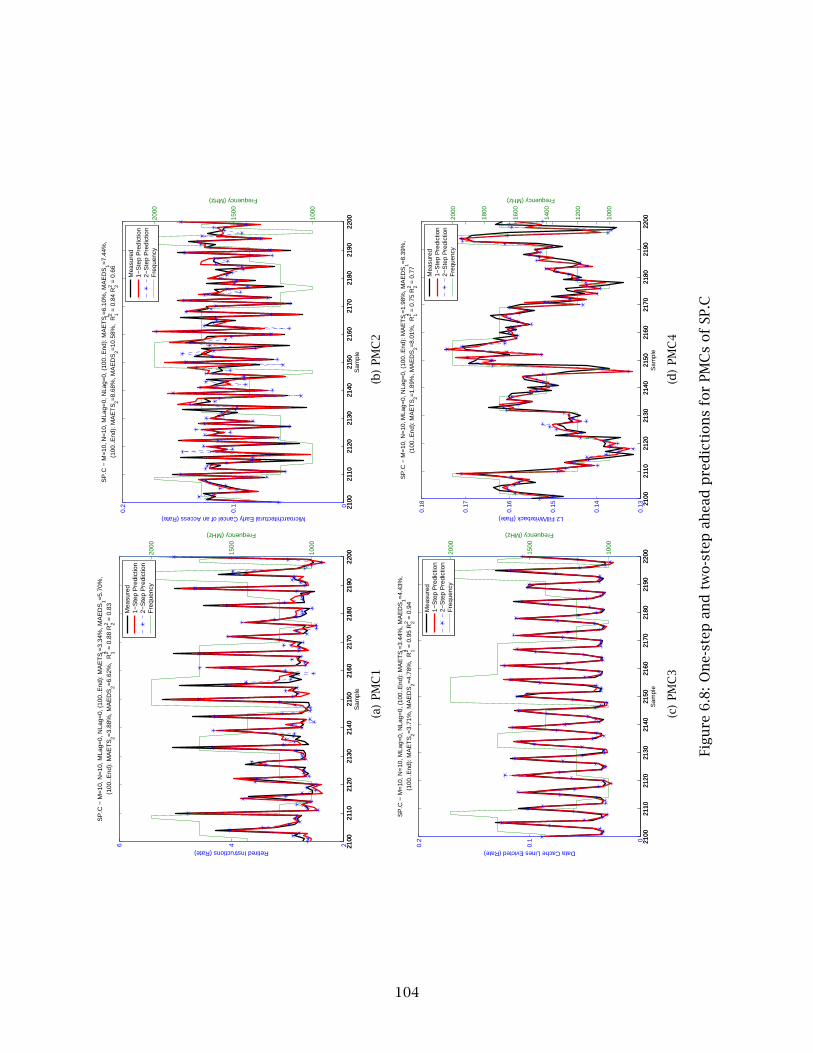
2100
2110
2120
2130
2140
2150
2160
2170
2180
2190
2200
246
Sam
ple
Retired Instructions (Rate)
SP
.C −
M=
10, N
=10
, MLa
g=0,
NLa
g=0,
(10
0..E
nd):
MA
ET
S 1=3.
34%
, MA
ED
S1=
5.70
%,
(100
..End
): M
AE
TS
2=3.
88%
, MA
ED
S2=
6.62
%,
R12 =
0.8
8 R
22 = 0
.83
2100
2110
2120
2130
2140
2150
2160
2170
2180
2190
220010
00
1500
2000
Frequency (MHz)
Mea
sure
d1−
Ste
p P
redi
ctio
n2−
Ste
p P
redi
ctio
nF
requ
ency
(a)
PM
C1
2100
2110
2120
2130
2140
2150
2160
2170
2180
2190
2200
0
0.1
0.2
Sam
ple
Microarchitectural Early Cancel of an Access (Rate)
SP
.C −
M=
10, N
=10
, MLa
g=0,
NLa
g=0,
(10
0..E
nd):
MA
ET
S 1=6.
10%
, MA
ED
S1=
7.44
%,
(100
..End
): M
AE
TS
2=8.
68%
, MA
ED
S2=
10.5
8%,
R12 =
0.8
4 R
22 = 0
.66
2100
2110
2120
2130
2140
2150
2160
2170
2180
2190
220010
00
1500
2000
Frequency (MHz)
Mea
sure
d1−
Ste
p P
redi
ctio
n2−
Ste
p P
redi
ctio
nF
requ
ency
(b)
PM
C2
2100
2110
2120
2130
2140
2150
2160
2170
2180
2190
2200
0
0.1
0.2
Sam
ple
Data Cache Lines Evicted (Rate)
SP
.C −
M=
10, N
=10
, MLa
g=0,
NLa
g=0,
(10
0..E
nd):
MA
ET
S 1=3.
44%
, MA
ED
S1=
4.43
%,
(100
..End
): M
AE
TS
2=3.
71%
, MA
ED
S2=
4.78
%,
R12 =
0.9
5 R
22 = 0
.94
2100
2110
2120
2130
2140
2150
2160
2170
2180
2190
220010
00
1500
2000
Frequency (MHz)
Mea
sure
d1−
Ste
p P
redi
ctio
n2−
Ste
p P
redi
ctio
nF
requ
ency
(c)
PM
C3
2100
2110
2120
2130
2140
2150
2160
2170
2180
2190
2200
0.13
0.14
0.15
0.16
0.17
0.18
Sam
ple
L2 Fill/Writeback (Rate)
SP
.C −
M=
10, N
=10
, MLa
g=0,
NLa
g=0,
(10
0..E
nd):
MA
ET
S 1=1.
98%
, MA
ED
S1=
8.39
%,
(100
..End
): M
AE
TS
2=1.
89%
, MA
ED
S2=
8.01
%,
R12 =
0.7
5 R
22 = 0
.77
2100
2110
2120
2130
2140
2150
2160
2170
2180
2190
220010
00
1200
1400
1600
1800
2000
Frequency (MHz)
Mea
sure
d1−
Ste
p P
redi
ctio
n2−
Ste
p P
redi
ctio
nF
requ
ency
(d)
PM
C4
Figu
re6.8
:O
ne-
step
and
two-s
tep
ahea
dp
red
icti
on
sfo
rPM
Cs
of
SP.C
104

200
210
220
230
240
250
260
270
280
290
300
01020
Sam
ple
Retired Instructions (Rate)
FT
.C −
M=
10, N
=10
, MLa
g=0,
NLa
g=0,
(10
0..E
nd):
MA
ET
S 1=9.
52%
, MA
ED
S1=
9.97
%,
(100
..End
): M
AE
TS
2=11
.30%
, MA
ED
S2=
11.8
3%,
R12 =
0.6
2 R
22 = 0
.52
200
210
220
230
240
250
260
270
280
290
30010
00
1500
2000
Frequency (MHz)
Mea
sure
d1−
Ste
p P
redi
ctio
n2−
Ste
p P
redi
ctio
nF
requ
ency
(a)
PM
C1
200
210
220
230
240
250
260
270
280
290
300
0
0.5
Sam
ple
Microarchitectural Early Cancel of an Access (Rate)
FT
.C −
M=
10, N
=10
, MLa
g=0,
NLa
g=0,
(10
0..E
nd):
MA
ET
S 1=6.
84%
, MA
ED
S1=
9.15
%,
(100
..End
): M
AE
TS
2=7.
68%
, MA
ED
S2=
10.2
7%,
R12 =
0.6
4 R
22 = 0
.59
200
210
220
230
240
250
260
270
280
290
30010
00
2000
Frequency (MHz)
Mea
sure
d1−
Ste
p P
redi
ctio
n2−
Ste
p P
redi
ctio
nF
requ
ency
(b)
PM
C2
200
210
220
230
240
250
260
270
280
290
300
0.00
5
0.01
0.01
5
0.02
0.02
5
0.03
Sam
ple
Data Cache Lines Evicted (Rate)
FT
.C −
M=
10, N
=10
, MLa
g=0,
NLa
g=0,
(10
0..E
nd):
MA
ET
S 1=7.
54%
, MA
ED
S1=
8.21
%,
(100
..End
): M
AE
TS
2=9.
03%
, MA
ED
S2=
9.83
%,
R12 =
0.4
8 R
22 = 0
.28
200
210
220
230
240
250
260
270
280
290
30010
00
1200
1400
1600
1800
2000
Frequency (MHz)
Mea
sure
d1−
Ste
p P
redi
ctio
n2−
Ste
p P
redi
ctio
nF
requ
ency
(c)
PM
C3
200
210
220
230
240
250
260
270
280
290
300
0
0.51
Sam
ple
L2 Fill/Writeback (Rate)
FT
.C −
M=
10, N
=10
, MLa
g=0,
NLa
g=0,
(10
0..E
nd):
MA
ET
S 1=9.
82%
, MA
ED
S1=
10.0
4%,
(100
..End
): M
AE
TS
2=11
.76%
, MA
ED
S2=
12.0
3%,
R12 =
0.6
3 R
22 = 0
.52
200
210
220
230
240
250
260
270
280
290
30010
00
1500
2000
Frequency (MHz)
Mea
sure
d1−
Ste
p P
redi
ctio
n2−
Ste
p P
redi
ctio
nF
requ
ency
(d)
PM
C4
Figu
re6.9
:O
ne-
step
and
two-s
tep
ahea
dp
red
icti
on
sfo
rPM
Cs
of
FT.C
105

100
110
120
130
140
150
160
170
180
190
200
4
4.55
5.56
6.5
Sam
ple
Retired Instructions (Rate)
MG
.C −
M=
10, N
=10
, MLa
g=0,
NLa
g=0,
(10
0..E
nd):
MA
ET
S1=
3.70
%, M
AE
DS
1=4.
04%
,(1
00..E
nd):
MA
ET
S2=
3.70
%, M
AE
DS
2=4.
04%
, R
12 = 0
.54
R22 =
0.5
0
100
110
120
130
140
150
160
170
180
190
20010
00
1200
1400
1600
1800
2000
Frequency (MHz)
Mea
sure
d1−
Ste
p P
redi
ctio
n2−
Ste
p P
redi
ctio
nF
requ
ency
(a)
PM
C1
100
110
120
130
140
150
160
170
180
190
200
0.2
0.4
0.6
Sam
ple
Microarchitectural Early Cancel of an Access (Rate)
MG
.C −
M=
10, N
=10
, MLa
g=0,
NLa
g=0,
(10
0..E
nd):
MA
ET
S1=
5.15
%, M
AE
DS
1=6.
66%
,(1
00..E
nd):
MA
ET
S2=
5.66
%, M
AE
DS
2=7.
32%
, R
12 = 0
.66
R22 =
0.5
6
100
110
120
130
140
150
160
170
180
190
20010
00
1500
2000
Frequency (MHz)
Mea
sure
d1−
Ste
p P
redi
ctio
n2−
Ste
p P
redi
ctio
nF
requ
ency
(b)
PM
C2
100
110
120
130
140
150
160
170
180
190
200
0
0.1
0.2
Sam
ple
Data Cache Lines Evicted (Rate)
MG
.C −
M=
10, N
=10
, MLa
g=0,
NLa
g=0,
(10
0..E
nd):
MA
ET
S1=
9.83
%, M
AE
DS
1=9.
85%
,(1
00..E
nd):
MA
ET
S2=
9.62
%, M
AE
DS
2=9.
64%
, R
12 = 0
.45
R22 =
0.4
8
100
110
120
130
140
150
160
170
180
190
20010
00
1500
2000
Frequency (MHz)
Mea
sure
d1−
Ste
p P
redi
ctio
n2−
Ste
p P
redi
ctio
nF
requ
ency
(c)
PM
C3
100
110
120
130
140
150
160
170
180
190
200
0.1
0.2
0.3
Sam
ple
L2 Fill/Writeback (Rate)
MG
.C −
M=
10, N
=10
, MLa
g=0,
NLa
g=0,
(10
0..E
nd):
MA
ET
S1=
5.27
%, M
AE
DS
1=5.
40%
,(1
00..E
nd):
MA
ET
S2=
5.10
%, M
AE
DS
2=5.
22%
, R
12 = 0
.58
R22 =
0.5
8
100
110
120
130
140
150
160
170
180
190
20010
00
1500
2000
Frequency (MHz)
Mea
sure
d1−
Ste
p P
redi
ctio
n2−
Ste
p P
redi
ctio
nF
requ
ency
(d)
PM
C4
Figu
re6.1
0:
On
e-st
epan
dtw
o-s
tep
ahea
dp
red
icti
on
sfo
rPM
Cs
of
MG
.C
106

One of the benefits of our general approach for PMC prediction, unlike other approaches
[23], is to be able to predict PMC events other than the IPC. The one-step and two-step ahead
predictions using an ARMAX(10, 0, 10) for a part of the signal of the IPC (labeled as PMC1),
Micro-architectural Early Cancel of an Access (labeled as PMC2), Data Cache Lines Evicted
(labeled as PMC3), and L2 Fill/Writeback (labeled as PMC4) for BT.C, LU.C, SP.C, FT.C, and MG.C
are shown in Figure 6.6, Figure 6.7, Figure 6.8, Figure 6.9, and Figure 6.10, respectively.
It is noticeable that FT.C and MG.C, which run only for a relatively short time, compared
to the other applications, BT.C, LU.C, and SP.C, follow the changes of the metrics closely in
shape, however, not as closely in terms of matching the signal levels (i.e., scale and offset) as
other applications. We believe that this is to due to the fact that the mean and variance of
the metrics calculated for each frequency, up to each time sample during the execution of the
application, have not converged to a stable region due to the lack of samples. For example, a
300 sample execution time running with five different frequencies only allocates approximately
60 samples by the end of the execution for calculation of mean and variance. An example
of unstable, but converging, mean and variance trends has been shown in Figure 5.9. Before
running each of the applications presented in this section, the initial mean and variance values
in the ZMUV module are reset to zero. This mismatch in scale and offset can be improved by
providing a longer mean and variance for the ZMUV module before running this application.
However, we choose to present to results here with a reset ZMUV module for the sake of a fair
comparison and focusing on the other aspects of prediction (e.g., application behavior and
ARMAX efficiency). In Section 6.3, we extend and utilize this PMC prediction model to predict
future power consumption of the system.
6.3 Power Prediction using ARMAX-RLS
In this section, we provide an ARMAX model for prediction of power consumption based on
previous PMC and power measurements.
107

6.3.1 Power Prediction Model
The problem formulation for power prediction is similar to the PMC prediction model. However,
this prediction model includes both power and PMC measurements as its inputs. Let P[t] and
cj[t] represent the power consumption and the jth PMC event rate (1 ≤ j ≤ nr ) measured at
time t, respectively. The previous power measurements P[t− i] are related to the current power
measurement P[t] via a coefficient βi. Similarly, the previous measurements of the jth PMC
event cj[t − i] are related to the current power measurement P[t] via a coefficient αi,j .
P[t] =m∑i=1
jmax∑j=1
αi,jcj[t − i]+n∑i=1
βiP[t − i] (6.4)
This model is presented in (6.4), where jmax = nr . At time step t the αi,j and βi
coefficients are updated using the RLS algorithm. Similar to the PMC prediction model notation,
we denote the updated coefficients at time step t via a superscript, such as in α(t)i,j and β(t)i .
We can use the obtained model at time t to perform a one-step ahead prediction of power
consumption as described in (6.5).
P[t + 1] =m∑i=1
jmax∑j=1
α(t)i,j cj[t + 1− i]+n∑i=1
β(t)i P[t + 1− i] (6.5)
A k-step ahead prediction of power consumption (k > 1) is performed using the PMC
prediction models and the power prediction model in parallel and recursively by performing k
one-step ahead predictions. We use the model obtained at time t and substitute the missing
power and PMC observations in time by their previously predicted values. This requires running
nr + 1 parallel models, nr for the prediction of the PMCs and one model for prediction of
power. The coefficients of the models are updated only at time t with real measurements. A
k-step ahead prediction model for power consumption is formulated in (6.6), where k ≤m,n.
This includes k − 1 previously predicted terms of cj and P, as well as their m − k + 1 and
n− k+ 1 latest observations of cj and P, respectively. The PMC predictions cj are calculated
using (6.2) and (6.3), discussed in Section 6.2.1. As discussed earlier in Section 4.5.3, the RLS
108

does not require any matrix inversion and can be implemented using matrix additions and
multiplications. The additional complexity of having the nr PMC models running in parallel
to the power model is not needed for obtaining the one-step ahead predictions, which many
resource managers need.
The ZMUV module adapts the power and PMC prediction methods proposed in this
chapter for a variable frequency environment. Similar to the PMC prediction model, all the
measured inputs in our proposed power prediction model (e.g., cj[t] and P[t]) are scaled
and offset to a unified frequency time-series using a ZMUV transformation (see Section 5.3).
The original values after performing predictions can be obtained by using an inverse ZMUV
transformation. The offline simulation results of our proposed power prediction model using
real system measurements in a variable frequency environment are presented in Section 6.3.2.
P[t + k] =k−1∑i=1
jmax∑j=1
α(t)i,j cj[t + k− i]+k−1∑i=1
β(t)i P[t + k− i]+ (6.6)
m∑i=k
jmax∑j=1
α(t)i,j cj[t + k− i]+n∑i=kβ(t)i P[t + k− i]
6.3.2 Power Prediction Results
In this section, we evaluate the efficiency of the power prediction method proposed in Section
6.3.1. We predict the power consumption of our system for BT.C, LU.C, SP.C, FT.C, and MG.C
running with eight threads in a variable frequency environment. We use a previously generated
random frequency pattern (duration and value) for all of the cores identically. We use the same
PMC events as in Section 6.2.2, which are IPC, Micro-architectural Early Cancel of an Access,
Data Cache Lines Evicted, and L2 Fill/Writeback. The PMC events are used as a system aggregate
metric, as opposed to a per core measurement. A summary of efficiency of one- and two-step
ahead power prediction using ARMAX(4, 0, 4) and ARMAX(10, 0, 10) models is provided in Table
6.5.
Our proposed power prediction method, when using the ARMAX(10, 0, 10) model,
provides the one-step ahead predictions of our test applications with a R2 of 0.63–0.72, a
MAEDS of 8.53–11.09%, and a MAETS of 2.57–3.34%. The two-step ahead power predictions
109

Table 6.5: Efficiency of variable frequency power consumption predictionsARMAX (4, 0, 4) (10, 0, 10) (4, 0, 4) (10, 0, 10) (4, 0, 4) (10, 0, 10)App./1-Step R2 R2 MAEDS% MAEDS% MAETS% MAETS%
BT.C 0.72 0.72 9.30 9.53 3.09 3.17LU.C 0.70 0.70 8.39 8.53 2.51 2.56SP.C 0.67 0.67 9.64 9.94 2.49 2.57FT.C 0.68 0.68 11.49 11.09 3.46 3.34MG.C 0.63 0.63 9.93 10.05 3.05 3.08
ARMAX (4, 0, 4) (10, 0, 10) (4, 0, 4) (10, 0, 10) (4, 0, 4) (10, 0, 10)App./2-Step R2 R2 MAEDS% MAEDS% MAETS% MAETS%
BT.C 0.60 0.61 12.12 12.01 4.03 3.99LU.C 0.53 0.54 11.09 11.14 3.32 3.34SP.C 0.52 0.53 12.07 12.15 3.12 3.14FT.C 0.67 0.69 11.32 10.86 3.41 3.27MG.C 0.64 0.63 9.86 9.79 3.03 3.00
using this model for our test applications performs with a R2 of 0.53–0.69, a MAEDS of 9.79–
12.15%, and a MAETS of 3.00–3.99%. The ARMAX(4, 0, 4) model in most cases performs similar
to the ARMAX(10, 0, 10) model and slightly better in some cases. A part of the one- and two-step
ahead power prediction for BT.C, LU.C, SP.C, FT.C, and MG.C using an ARMAX(10, 0, 10) model
is presented in Figure 6.11, Figure 6.12, Figure 6.13, Figure 6.14, and Figure 6.15, respectively.
110

1500 1510 1520 1530 1540 1550 1560 1570 1580 1590 1600200
300
400
Sample
Pow
er (
Wat
ts)
BT.C − M=10, N=10, MLag=0, NLag=0, (100..End): MAETS1=3.17%, MAEDS
1=9.53%,
(100..End): MAETS2=3.99%, MAEDS
2=12.01%, R
12 = 0.72 R
22 = 0.61
1500 1510 1520 1530 1540 1550 1560 1570 1580 1590 1600
1000
1500
2000
Fre
quen
cy (
MH
z)
Measured1−Step Prediction2−Step PredictionFrequency
Figure 6.11: One-step and two-step ahead predictions for power consumption of BT.C
2300 2310 2320 2330 2340 2350 2360 2370 2380 2390 2400200
220
240
260
280
300
Sample
Pow
er (
Wat
ts)
LU.C − M=10, N=10, MLag=0, NLag=0, (100..End): MAETS1=2.56%, MAEDS
1=8.53%,
(100..End): MAETS2=3.34%, MAEDS
2=11.14%, R
12 = 0.70 R
22 = 0.54
2300 2310 2320 2330 2340 2350 2360 2370 2380 2390 2400
1000
1200
1400
1600
1800
2000
Fre
quen
cy (
MH
z)
Measured1−Step Prediction2−Step PredictionFrequency
Figure 6.12: One-step and two-step ahead predictions for power consumption of LU.C
111
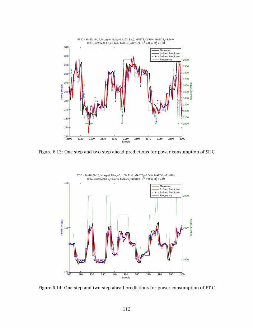
2100 2110 2120 2130 2140 2150 2160 2170 2180 2190 2200210
220
230
240
250
260
270
280
290
300
310
Sample
Pow
er (
Wat
ts)
SP.C − M=10, N=10, MLag=0, NLag=0, (100..End): MAETS1=2.57%, MAEDS
1=9.94%,
(100..End): MAETS2=3.14%, MAEDS
2=12.15%, R
12 = 0.67 R
22 = 0.53
2100 2110 2120 2130 2140 2150 2160 2170 2180 2190 2200
1000
1100
1200
1300
1400
1500
1600
1700
1800
1900
2000
Fre
quen
cy (
MH
z)
Measured1−Step Prediction2−Step PredictionFrequency
Figure 6.13: One-step and two-step ahead predictions for power consumption of SP.C
200 210 220 230 240 250 260 270 280 290 300200
300
400
Sample
Pow
er (
Wat
ts)
FT.C − M=10, N=10, MLag=0, NLag=0, (100..End): MAETS1=3.34%, MAEDS
1=11.09%,
(100..End): MAETS2=3.27%, MAEDS
2=10.86%, R
12 = 0.68 R
22 = 0.69
200 210 220 230 240 250 260 270 280 290 300
1000
1500
2000
Fre
quen
cy (
MH
z)
Measured1−Step Prediction2−Step PredictionFrequency
Figure 6.14: One-step and two-step ahead predictions for power consumption of FT.C
112

100 110 120 130 140 150 160 170 180 190 200200
250
300
Sample
Pow
er (
Wat
ts)
MG.C − M=10, N=10, MLag=0, NLag=0, (100..End): MAETS1=3.08%, MAEDS
1=10.05%,
(100..End): MAETS2=3.00%, MAEDS
2=9.79%, R
12 = 0.63 R
22 = 0.63
100 110 120 130 140 150 160 170 180 190 200
1000
1500
2000
Fre
quen
cy (
MH
z)
Measured1−Step Prediction2−Step PredictionFrequency
Figure 6.15: One-step and two-step ahead predictions for power consumption of MG.C
113

6.4 IPC Prediction in Real Time
We have implemented the PMC prediction model that is introduced in Section 6.2 in a real-time
environment. The results of this real-time implementation confirm the results of the study
in Section 6.2 that were obtained at a simulation level. The prediction code 1 is written in
C/C++ and is able to predict PMC events, such as IPC. We have chosen the input PMC events for
this multivariate time-series prediction model to be IPC, Micro-architectural Early Cancel of an
Access, Data Cache Lines Evicted, and L2 Fill/Writeback.
We run a number of multi-threaded NPB-OMP applications in a row as a real test for our
prediction program. We have included a delay between some of our applications to include
the effect of idle periods in the PMC predictions. The order of sleep periods and application
executions are as the following: we start with a 2-second sleep period, followed by BT.A, CG.A,
EP.A, FT.A, IS.A, LU.A, MG.A, SP.A, a 2-second sleep period, BT.B, a 2-second sleep period, FT.B, a
2-second sleep period, LU.B, a 2-second sleep period, MG.B, a 2-second sleep period, SP.B, and a
2-second sleep period. The predicted values include the activity of all the threads and processes
running on the system, including the operating system, ARMAX-RLS predicting program, and
the test benchmark applications.
The frequency of all cores are simultaneously changed to a previously generated random
frequency pattern. In this test, we are measuring four PMC events on the eight available cores.
It is expected that for a time-series prediction approach, such as the ARMAX-RLS, the prediction
error for the further time steps to be larger. Moreover, a dynamic resource management system
commonly requires only the predictions of a few steps ahead to transform its reactive scheme
into a proactive algorithm. Thus, we limit the prediction horizon of this real-time application
to two time steps ahead. We perform one- and two-step ahead PMC predictions using an
ARMAX(10, 0, 10) for each core using its PMC measurements. Furthermore, we perform a similar
PMC prediction on the system using the average of each PMC event of all of the cores that we
refer to average here. As the predictions for each PMC event is calculated using its own model,
for the average system and eight cores a total of 36 models are running simultaneously. If only
1The transformation of Matlab code to C/C++ code was performed collaboratively with Ryan Patrick Andersonand Mike Mallin, the undergraduate research assistants at the Parallel Processing Research Laboratory, Departmentof Electrical and Computer Engineering, Queen’s University.
114

the one-step ahead predictions of one PMC event are needed, we can reduce this number of
parallel models running on the system to one model per core. If one is only interested in the
overall system prediction, the per core prediction models can be disabled as well and leaving
only one model running on the system. Such a versatile module can be utilized for different
purposes, including power saving methods based on PMC metrics [23, 146]. We present the
prediction results of the run-time PMCs in two sections. In Sections 6.4.1, we provide the
real-time predictions of the aggregate PMC events of all cores (average). Section 6.4.2 presents
the real-time IPC prediction of each core on our system.
6.4.1 Aggregate PMCs
A summary of the predictions efficiency metrics of the aggregate PMC events at run-time using
an ARMAX(10, 0, 10) model is provided in Table 6.6. The PMC events used for this test are IPC
(labeled as PMC1), Micro-architectural Early Cancel of an Access (labeled as PMC2), Data Cache
Lines Evicted (labeled as PMC3), and L2 Fill/Writeback (labeled as PMC4). We also compare the
prediction efficiency metrics of our ARMAX model to a last value predictor, denoted as LAST.
The one-step ahead prediction of all the PMC events are performed with a R2 of 0.56–
0.68, a MAEDS of 3.49–6.24%, and a MAETS of 3.49–6.20%. The two-step ahead prediction
of all the PMC events using the ARMAX model perform with a R2 of 0.24–0.59, a MAEDS of
4.20–6.98%, and a MAETS of 4.20–6.94%. The LAST predictor does not provide a good R2 for
power prediction. The ARMAX model provides 24–50% (23% for IPC) smaller errors than the
LAST predictor for one-step ahead predictions. The error reduction of ARMAX compared to the
LAST predictor is 21–41% (26% for IPC) for two-step ahead predictions. A part of the real-time
IPC prediction of this multi-application test is shown in Figure 6.16 and Figure 6.17. Similarly, a
part of the real-time predictions for L2 Fill/Writeback is shown in Figure 6.18 and Figure 6.19.
115

0 10 20 30 40 50 60 70 80 90 1000
1
Sample
PM
C (
Rat
e)
Multi−App. − M=10, N=10, MLag=0, NLag=0, (100..End): MAETS1=5.65%, MAEDS
1=5.70%,
(100..End): MAETS2=6.69%, MAEDS
2=6.75%, R
12 = 0.68 R
22 = 0.49
0 10 20 30 40 50 60 70 80 90 100
1000
1500
2000
Fre
quen
cy (
MH
z)
Measured 1−Step Prediction 2−Step Prediction Frequency
100 110 120 130 140 150 160 170 180 190 2000
1
Sample
PM
C (
Rat
e)
100 110 120 130 140 150 160 170 180 190 200
1000
1500
2000
Fre
quen
cy (
MH
z)
200 210 220 230 240 250 260 270 280 290 3000
1
Sample
PM
C (
Rat
e)
200 210 220 230 240 250 260 270 280 290 300
1000
1500
2000
Fre
quen
cy (
MH
z)
Figure 6.16: One-step and two-step ahead real time predictions for IPC (set 1)
300 310 320 330 340 350 360 370 380 390 4000
1
Sample
PM
C (
Rat
e)
Multi−App. − M=10, N=10, MLag=0, NLag=0, (100..End): MAETS1=5.65%, MAEDS
1=5.70%,
(100..End): MAETS2=6.69%, MAEDS
2=6.75%, R
12 = 0.68 R
22 = 0.49
300 310 320 330 340 350 360 370 380 390 400
1000
1500
2000
Fre
quen
cy (
MH
z)
Measured 1−Step Prediction 2−Step Prediction Frequency
400 410 420 430 440 450 460 470 480 490 5000
1
Sample
PM
C (
Rat
e)
400 410 420 430 440 450 460 470 480 490 500
1000
1500
2000
Fre
quen
cy (
MH
z)
500 510 520 530 540 550 560 570 580 590 6000
1
Sample
PM
C (
Rat
e)
500 510 520 530 540 550 560 570 580 590 600
1000
1500
2000
Fre
quen
cy (
MH
z)
Figure 6.17: One-step and two-step ahead real time predictions for IPC (set 2)
116

0 10 20 30 40 50 60 70 80 90 1000
0.01
0.02
Sample
PM
C (
Rat
e)
Multi−App. − M=10, N=10, MLag=0, NLag=0, (100..End): MAETS1=3.49%, MAEDS
1=3.49%,
(100..End): MAETS2=4.20%, MAEDS
2=4.20%, R
12 = 0.56 R
22 = 0.24
0 10 20 30 40 50 60 70 80 90 100
1000
1500
2000
Fre
quen
cy (
MH
z)
Measured 1−Step Prediction 2−Step Prediction Frequency
100 110 120 130 140 150 160 170 180 190 2000
0.01
0.02
Sample
PM
C (
Rat
e)
100 110 120 130 140 150 160 170 180 190 200
1000
1500
2000
Fre
quen
cy (
MH
z)
200 210 220 230 240 250 260 270 280 290 300−0.05
0
0.05
Sample
PM
C (
Rat
e)
200 210 220 230 240 250 260 270 280 290 300
1000
1500
2000
Fre
quen
cy (
MH
z)
Figure 6.18: One-step and two-step ahead real time predictions for L2 Fill/Writeback (set 1)
300 310 320 330 340 350 360 370 380 390 400−0.1
−0.050
0.050.1
0.15
Sample
PM
C (
Rat
e)
Multi−App. − M=10, N=10, MLag=0, NLag=0, (100..End): MAETS1=3.49%, MAEDS
1=3.49%,
(100..End): MAETS2=4.20%, MAEDS
2=4.20%, R
12 = 0.56 R
22 = 0.24
300 310 320 330 340 350 360 370 380 390 400
100012001400160018002000
Fre
quen
cy (
MH
z)
Measured 1−Step Prediction 2−Step Prediction Frequency
400 410 420 430 440 450 460 470 480 490 5000
0.05
0.1
Sample
PM
C (
Rat
e)
400 410 420 430 440 450 460 470 480 490 500
1000
1500
2000
Fre
quen
cy (
MH
z)
500 510 520 530 540 550 560 570 580 590 6000
0.05
0.1
Sample
PM
C (
Rat
e)
500 510 520 530 540 550 560 570 580 590 600
1000
1500
2000
Fre
quen
cy (
MH
z)
Figure 6.19: One-step and two-step ahead real time predictions for L2 Fill/Writeback (set 2)
117

Table 6.6: Efficiency of variable frequency real time aggregate PMC predictionModel ARMAX LAST ARMAX LAST ARMAX LASTPMC/1-Step R2 R2 MAEDS% MAEDS% MAETS% MAETS%
PMC1 0.68 0.47 5.70 7.45 5.65 7.39PMC2 0.68 0.08 6.24 10.56 6.20 10.50PMC3 0.61 -0.49 4.95 10.15 4.95 10.15PMC4 0.56 0.39 3.49 4.68 3.49 4.67
Model ARMAX LAST ARMAX LAST ARMAX LASTPMC/2-Step R2 R2 MAEDS% MAEDS% MAETS% MAETS%
PMC1 0.49 0.23 6.75 9.17 6.69 9.09PMC2 0.59 -0.10 6.98 11.75 6.94 11.67PMC3 0.46 -0.07 5.90 8.23 5.90 8.23PMC4 0.24 0.20 4.20 5.35 4.20 5.35
6.4.2 Per Core PMCs
In this section, we evaluate the efficiency of the ARMAX model in predicting the per core
PMC events, as well as the system aggregate PMCs (average). We use an ARMAX(10, 0, 10)
model for this section in a variable frequency environment. The PMC events predicted in this
section are IPC, Micro-architectural Early Cancel of an Access, Data Cache Lines Evicted, and L2
Fill/Writeback. Table 6.7 provides the details of the efficiency metrics of one-step ahead PMC
predictions.
For IPC, all the cores and the aggregate system provide a R2 of 0.67–0.71, a MAEDS of
5.39–5.99%, and a MAETS of 5.38–5.99%. For Micro-architectural Early Cancel of an Access,
the per core and aggregate prediction efficiency metrics have a R2 of 0.61–0.70, a MAEDS of
4.84–6.49%, and a MAETS of 4.84–6.49%. For Data Cache Lines Evicted, the per core/aggregate
prediction efficiency metrics are R2 of 0.59–0.69, MAEDS of 3.71–8.22%, and MAETS of 3.71–
8.22%. Finally, for L2 Fill/Writeback, the per core/aggregate prediction efficiency metrics are
R2 of 0.43–0.62, MAEDS of 3.20–3.84%, and MAETS of 3.20–3.84%. The efficiency metrics of
prediction for most cores and the system aggregate are mostly similar to each other. For all
of the per cores/aggregate predictions, the ARMAX model outperforms the LAST predictor
significantly. The are many different applications, such as power saving and dynamic scheduling
algorithms, that can benefit from such a run-time prediction system.
118

Table 6.7: Efficiency of aggregate and per core one-step ahead PMC predictionsIPC
Model ARMAX LAST ARMAX LAST ARMAX LASTCore/1-Step R2 R2 MAEDS% MAEDS% MAETS% MAETS%Average 0.68 0.47 5.70 7.45 5.65 7.39Core 0 0.71 0.49 5.69 7.39 5.69 7.39Core 1 0.68 0.37 5.39 7.41 5.38 7.41Core 2 0.67 0.52 5.79 7.15 5.79 7.14Core 3 0.67 0.44 5.76 7.70 5.75 7.70Core 4 0.68 0.47 5.95 7.84 5.94 7.84Core 5 0.68 0.45 5.89 7.70 5.89 7.70Core 6 0.67 0.47 5.99 7.82 5.99 7.82Core 7 0.67 0.45 5.92 7.66 5.92 7.65
Micro-architectural Early Cancel of an AccessCore/1-Step R2 R2 MAEDS% MAEDS% MAETS% MAETS%Average 0.68 0.08 6.24 10.56 6.20 10.50Core 0 0.64 0.15 5.59 8.76 5.58 8.76Core 1 0.61 0.23 5.22 7.93 5.22 7.92Core 2 0.70 0.28 4.84 7.86 4.84 7.86Core 3 0.69 0.07 5.52 9.70 5.52 9.69Core 4 0.66 0.08 6.00 9.93 6.00 9.92Core 5 0.66 0.14 6.49 10.23 6.49 10.22Core 6 0.65 0.05 5.79 9.64 5.79 9.64Core 7 0.72 0.16 5.84 9.95 5.84 9.94
Data Cache Lines EvictedCore/1-Step R2 R2 MAEDS% MAEDS% MAETS% MAETS%Average 0.61 -0.49 4.95 10.15 4.95 10.15Core 0 0.62 -0.46 3.85 7.81 3.85 7.80Core 1 0.60 -0.39 3.85 7.40 3.85 7.40Core 2 0.69 -0.18 7.40 15.14 7.40 15.14Core 3 0.66 -0.41 8.22 17.09 8.22 17.09Core 4 0.59 -0.46 3.71 7.44 3.71 7.44Core 5 0.63 -0.52 4.93 10.16 4.93 10.16Core 6 0.60 -0.48 3.74 7.59 3.74 7.59Core 7 0.63 -0.58 6.51 13.40 6.51 13.40
L2 Fill/WritebackCore/1-Step R2 R2 MAEDS% MAEDS% MAETS% MAETS%Average 0.56 0.39 3.49 4.68 3.49 4.67Core 0 0.59 0.41 3.51 4.67 3.51 4.67Core 1 0.62 0.44 3.20 4.05 3.20 4.05Core 2 0.55 0.45 3.54 4.57 3.54 4.57Core 3 0.60 0.48 3.84 5.12 3.84 5.12Core 4 0.55 0.35 3.58 4.79 3.58 4.79Core 5 0.56 0.35 3.64 4.94 3.64 4.94Core 6 0.55 0.35 3.67 4.94 3.67 4.94Core 7 0.43 0.32 3.66 4.84 3.66 4.84
119

6.5 Discussion
Given the need for increased efficiency in the current computing systems, having access to
predicted values of different metrics of the system becomes significantly important. Power
reduction can become a trivial task of changing voltage and frequency if one has accurate
predictions of the upcoming workload and system state. We have used the ARMAX-RLS model
to show that it is possible to obtain run-time prediction of different PMC events, such as IPC, in a
variable frequency environment. Furthermore, using the ARMAX-RLS one can predict the power
consumption of the system in a variable frequency environment. For both PMC and power,
many steps of predictions can be made ahead of time. We have shown that our ARMAX-RLS
predictors significantly outperform the last value predictors, which are commonly used. Finally,
we have implemented the PMC prediction model proposed in this chapter on a real multicore
system. For example, one-step ahead of time, we are able to predict the per core or aggregate
PMC rates of IPC, Micro-architectural Early Cancel of an Access, Data Cache Lines Evicted, and
L2 Fill/Writeback with a MAETS of 5.4–6.0%, 4.8–6.5%, 3.7–8.2%, and 3.2–3.8%, respectively.
120

Chapter 7
Conclusions and Future Work
Architectural intuition has guided many prior work to choose PMC events in a power model.
However, a comprehensive statistical analysis of PMC event selection has been missing prior
to this work. The proposed method for efficient selection of an optimal set of PMC events for
power modeling purposes requires six times less number of executions than a PCA method. Our
proposed method does not suffer from inaccuracies incurred by assuming that the statistics
of power consumption and PMCs for different processes or threads of a parallel application
are identical among different cores or nodes. This helps power models to incorporate useful
information of the system, through the limited number of available PMC registers, with minimal
overlap of information provided by different measured PMC events. We have shown that the
most significant PMC events in an application, or a group of applications, are not necessarily
the same as the ones arbitrarily chosen by architectural intuitions.
We exploit the intrinsic repetitiveness of computer software and hardware through the
time dependence between the measured metrics of a system to develop a power model. We
have shown that combining a linear model between the activity of a system and its power
consumption with the time dependence of data within each metric signal (i.e., power or PMC),
in addition to the time dependence of data between the signals, can provide an accurate power
estimation model. To prepare this model as a run-time estimation method, we equip the
multivariate time-series model with a coefficient update algorithm to be able to adjust to the
changes in a system. In particular, we use an autoregressive moving average with exogenous
inputs jointly used with a coefficient update algorithm [151], such as KF, MVNR, and RLS. We
have shown that ARMAX-RLS is a suitable candidate for adaptive run-time power estimation
that is both architecture and application independent. The minimal computational overhead
121

and superior performance of RLS algorithm, compared to other algorithms such as Kalman
filter and MVNR, provide us with an adaptive module that is suitable for on-the-fly run-time
modeling of real systems.
The impact of frequency scaling on PMC and power metrics rules out many existing
models for integration in a real system for run-time estimation and prediction of metrics. Unlike
many prior works that use a regression method to capture the impact of frequency scaling in
the system metrics and differentiating between scaling and non-scaling metrics, our approach
is based on a practical Gaussian approximation [150]. Prior methods suffer from being able
to model only a limited set of PMCs that fit the theoretical model, which mostly represents
an oversimplified version of a real system or workload. We use the Gaussian distribution
properties with an attempt to make a variable frequency trend of a metric that is closer to
a weakly stationary signal. We scale and offset the metrics by their the mean and variance
associated to each frequency into a unified trend with a zero mean and unit variance. Our
approach is adaptive and does not dictate the usage of any specific PMC event. We have
shown that accurate power estimation of a real system in a variable frequency environment is
achievable through an ARMAX-RLS model when equipped with a ZMUV module.
In addition, we have extended our ARMAX-RLS model that is equipped with a ZMUV
module, to predict the near future PMCs and power consumption of a system in a variable
frequency environment. Unlike prior work that focuses on the univariate time-series methods
under a fixed frequency environment, or prediction of metrics that are insensitive to DVFS,
such as the system load and processor utilization, we have provided a generic methodology for
predicting power consumption and PMC events in a variable frequency environment. We have
shown that per core or aggregate system PMC event predictions multiple-steps ahead of time
is feasible using a multivariate time-series model, such as the ARMAX-RLS. Such a prediction
method can be used by resource managers to increase the efficiency of the system. For example,
we have shown that IPC can be predicted with a small error, one or two steps ahead of time,
which can be used in power saving algorithms suggested by others. The prediction of metrics
can also be used in improving dynamic scheduling algorithms from the power or performance
aspects. Overall, obtaining a reliable prediction of the system metrics is crucial for progressing
from a reactive power and performance management method to a proactive algorithm.
122

7.1 Future Work
First, we would like to perform a comprehensive study on different types of applications with
regard to the selection of the best PMCs for power modeling purposes. We would like to provide
a group of PMCs that are representative of a large set of various applications. This can be
beneficial for those who would like to skip the statistical PMC selection step and not to be
forced into picking intuition based PMC events.
In order to evaluate the efficiency of our approaches in a frequency variable environment,
we have changed the frequency of all eight cores in our system simultaneously according to a
previously generated random frequency pattern (duration and value). However, we have chosen
to have an identical frequency for all of the cores in the system at any time, in order to avoid
any system load imbalance. We would like to study the impact of possible load imbalance
when non-identical frequencies are used for the different cores in a system, with respect to the
efficiency of our ARMAX-RLS prediction and estimation methods.
In addition, we would like to study the usage of other time-series models, such as an
ARIMAX model, to see if we can gain any improvements in our estimations or predictions.
Moreover, we have chosen the MA terms of our ARMAX to be zero throughout this thesis. We
would like to explore more the impact of including MA terms in efficiency of our ARMAX model.
The goal of this thesis has been to facilitate building models and metrics that accurately
represent the current and future state of the system. Power management systems, which have
not been the primary focus of this thesis, are among the objectives that can benefit from a
prediction system like the ARMAX-RLS. Given an accurate prediction of the related metrics to
power saving opportunities, one can trivially change the frequency and voltage of a processor
for saving power with minimal performance degradation. As an extension to this work, we
would like to explore different power saving algorithms that use our prediction system.
123

References
[1] Advanced Configuration and Power Interface Specification. www.acpi.info, December
2011.
[2] Advanced Micro Devices (AMD). BIOS and kernel developer’s guide (BKDG) for AMD family
10h processors. Technical report, April 2011. 31116 Rev 3.48.
[3] K. Agrawal, Y. He, W. J. Hsu, and C. E. Leiserson. Adaptive scheduling with parallelism
feedback. In Proceedings of the eleventh ACM SIGPLAN symposium on Principles and
practice of parallel programming, PPoPP ’06, pages 100–109, New York, NY, USA, 2006.
ACM. ISBN 1-59593-189-9. doi: 10.1145/1122971.1122988.
[4] B. D. O. Anderson. Optimal Filtering. Prentice-Hall, 1979.
[5] N. S. Arora, R. D. Blumofe, and C. G. Plaxton. Thread scheduling for multiprogrammed
multiprocessors. In Proceedings of the tenth annual ACM symposium on Parallel algo-
rithms and architectures, SPAA ’98, pages 119–129, New York, NY, USA, 1998. ACM. ISBN
0-89791-989-0. doi: 10.1145/277651.277678.
[6] R. Azimi. System Software Utilization of Hardware Performance Monitoring Information.
PhD thesis, University of Toronto, 2007.
[7] R. Azimi, M. Stumm, and R. W. Wisniewski. Online performance analysis by statistical
sampling of microprocessor performance counters. In Proceedings of the 19th annual
international conference on Supercomputing, ICS ’05, pages 101–110, New York, NY, USA,
2005. ACM. ISBN 1-59593-167-8. doi: 10.1145/1088149.1088163.
[8] E. Bair, T. Hastie, D. Paul, and R. Tibshirani. Prediction by supervised principal components.
Journal of the American Statistical Association, 101(473):119–137, 2006. doi: 10.1198/
016214505000000628.
[9] S.-Y. Bang, K. Bang, S. Yoon, and E.-Y. Chung. Run-time adaptive workload estimation for
dynamic voltage scaling. Computer-Aided Design of Integrated Circuits and Systems, IEEE
Transactions on, 28(9):1334–1347, September 2009. ISSN 0278-0070. doi: 10.1109/TCAD.
2009.2024706.
[10] L. A. Barroso. The price of performance. Queue, 3(7):48–53, September 2005. ISSN
1542-7730. doi: 10.1145/1095408.1095420.
124

[11] J. Beecroft, D. Addison, D. Hewson, M. McLaren, D. Roweth, F. Petrini, and J. Nieplocha.
QSNET II: defining high-performance network design. Micro, IEEE, 25(4):34–47, July–
August 2005. ISSN 0272-1732. doi: 10.1109/MM.2005.75.
[12] F. Bellosa. The benefits of event: driven energy accounting in power-sensitive systems. In
Proceedings of the 9th workshop on ACM SIGOPS European workshop: beyond the PC: new
challenges for the operating system, EW 9, pages 37–42, New York, NY, USA, 2000. ACM.
[13] W. L. Bircher and L. John. Predictive power management for multi-core processors. In
Proceedings of the 2010 international conference on Computer Architecture, ISCA’10,
pages 243–255, Berlin, Heidelberg, 2012. Springer-Verlag. ISBN 978-3-642-24321-9. doi:
10.1007/978-3-642-24322-6_21.
[14] W. L. Bircher and L. K. John. Analysis of dynamic power management on multi-core pro-
cessors. In Proceedings of the 22nd annual international conference on Supercomputing,
ICS ’08, pages 327–338, New York, NY, USA, 2008. ACM. ISBN 978-1-60558-158-3. doi:
10.1145/1375527.1375575.
[15] W. L. Bircher, M. Valluri, J. Law, and L. K. John. Runtime identification of microprocessor
energy saving opportunities. In International Symposium on Low power electronics and
design, pages 275–280, 2005. ISBN 1-59593-137-6.
[16] S. Borkar and A. A. Chien. The future of microprocessors. Commun. ACM, 54(5):67–77,
May 2011. ISSN 0001-0782. doi: 10.1145/1941487.1941507.
[17] D. Bovet and M. Cesati. Understanding the Linux Kernel, Second Edition. O’Reilly &
Associates, Inc., Sebastopol, CA, USA, 2nd edition, 2002. ISBN 0596002130.
[18] D. Brooks, V. Tiwari, and M. Martonosi. Wattch: a framework for architectural-level power
analysis and optimizations. In Proceedings of the 27th annual international symposium
on Computer architecture, ISCA ’00, pages 83–94, New York, NY, USA, 2000. ACM. ISBN
1-58113-232-8. doi: 10.1145/339647.339657.
[19] J. A. Butts and G. S. Sohi. A static power model for architects. In Proceedings of the 33rd
annual ACM/IEEE international symposium on Microarchitecture, MICRO 33, pages 191–
201, New York, NY, USA, 2000. ACM. ISBN 1-58113-196-8. doi: 10.1145/360128.360148.
[20] F. Cappello and D. Etiemble. MPI versus MPI+OpenMP on IBM SP for the NAS benchmarks.
In Proceedings of the 2000 ACM/IEEE conference on Supercomputing, Supercomputing ’00,
Washington, DC, USA, 2000. IEEE Computer Society. ISBN 0-7803-9802-5.
[21] J. Carulli, J.M. and T. Anderson. The impact of multiple failure modes on estimating
product field reliability. Design Test of Computers, IEEE, 23(2):118–126, March–April 2006.
ISSN 0740-7475. doi: 10.1109/MDT.2006.53.
125

[22] R. Chen, L. Yang, and C. Hafner. Nonparametric multistep-ahead prediction in time series
analysis. Journal of the Royal Statistical Society: Series B (Statistical Methodology), 66(3):
669–686, 2004. ISSN 1467-9868. doi: 10.1111/j.1467-9868.2004.04664.x.
[23] S. Chheda, O. Unsal, I. Koren, C. M. Krishna, and C. A. Moritz. Combining compiler and
runtime IPC predictions to reduce energy in next generation architectures. In Proceedings
of the 1st conference on Computing frontiers, CF ’04, pages 240–254, New York, NY, USA,
2004. ACM. ISBN 1-58113-741-9. doi: 10.1145/977091.977125.
[24] Y. Cho, Y. Kim, S. Park, and N. Chang. System-level power estimation using an on-chip
bus performance monitoring unit. In ICCAD ’08: Proceedings of the 2008 IEEE/ACM
International Conference on Computer-Aided Design, pages 149–154, 2008. ISBN 978-1-
4244-2820-5.
[25] G. Contreras and M. Martonosi. Power prediction for Intel XScale processors using
performance monitoring unit events. In ISLPED ’05: Proceedings of the 2005 international
symposium on Low power electronics and design, pages 221–226. ACM, 2005. ISBN
1-59593-137-6.
[26] P. Conway, N. Kalyanasundharam, G. Donley, K. Lepak, and B. Hughes. Cache hierarchy and
memory subsystem of the AMD Opteron processor. Micro, IEEE, 30(2):16–29, March–April
2010. ISSN 0272-1732. doi: 10.1109/MM.2010.31.
[27] A. Coskun, T. Rosing, and K. Gross. Proactive temperature balancing for low cost thermal
management in MPSoCs. In Computer-Aided Design, 2008. ICCAD 2008. IEEE/ACM
International Conference on, pages 250–257, November 2008. doi: 10.1109/ICCAD.2008.
4681582.
[28] A. Coskun, J. Ayala, D. Atienza, and T. Rosing. Modeling and dynamic management
of 3D multicore systems with liquid cooling. In Very Large Scale Integration (VLSI-
SoC), 2009 17th IFIP International Conference on, pages 35–40, October 2009. doi:
10.1109/VLSISOC.2009.6041327.
[29] A. K. Coskun, D. Atienza, T. S. Rosing, T. Brunschwiler, and B. Michel. Energy-efficient
variable-flow liquid cooling in 3D stacked architectures. In Proceedings of the Conference
on Design, Automation and Test in Europe, DATE ’10, pages 111–116, 3001 Leuven,
Belgium, 2010. European Design and Automation Association. ISBN 978-3-9810801-6-2.
[30] M. Curtis-Maury, F. Blagojevic, C. Antonopoulos, and D. Nikolopoulos. Prediction-based
power-performance adaptation of multithreaded scientific codes. Parallel and Distributed
Systems, IEEE Transactions on, 19(10):1396–1410, October 2008. ISSN 1045-9219.
[31] M. Curtis-Maury, A. Shah, F. Blagojevic, D. S. Nikolopoulos, B. R. de Supinski, and M. Schulz.
Prediction models for multi-dimensional power-performance optimization on many
126

cores. In Proceedings of the 17th international conference on Parallel architectures and
compilation techniques, PACT ’08, pages 250–259, New York, NY, USA, 2008. ACM. ISBN
978-1-60558-282-5. doi: 10.1145/1454115.1454151.
[32] M. F. Curtis-Maury. Improving the Efficiency of Parallel Applications on Multithreaded and
Multicore Systems. PhD thesis, Virginia Polytechnic Institute and State University, March
2008.
[33] G. Dhiman, K. Mihic, and T. Rosing. A system for online power prediction in virtualized
environments using Gaussian mixture models. In Design Automation Conference (DAC),
2010 47th ACM/IEEE, pages 807–812, June 2010.
[34] Q. Diao and J. Song. Prediction of CPU idle-busy activity pattern. In High Performance
Computer Architecture, 2008. HPCA 2008. IEEE 14th International Symposium on, pages
27–36, February 2008. doi: 10.1109/HPCA.2008.4658625.
[35] R. P. Dick. Reliability, thermal, and power modeling and optimization. In Proceedings
of the International Conference on Computer-Aided Design, ICCAD ’10, pages 181–184,
Piscataway, NJ, USA, 2010. IEEE Press. ISBN 978-1-4244-8192-7.
[36] P. Dinda. Design, implementation, and performance of an extensible toolkit for resource
prediction in distributed systems. Parallel and Distributed Systems, IEEE Transactions on,
17(2):160–173, February 2006. ISSN 1045-9219. doi: 10.1109/TPDS.2006.24.
[37] P. Dinda. Online prediction of the running time of tasks. In High Performance Distributed
Computing, 2001. Proceedings. 10th IEEE International Symposium on, pages 383–394,
2001. doi: 10.1109/HPDC.2001.945206.
[38] P. A. Dinda and D. R. O’Hallaron. Host load prediction using linear models. Cluster Com-
puting, 3(4):265–280, October 2000. ISSN 1386-7857. doi: 10.1023/A:1019048724544.
[39] E. Duesterwald, C. Cascaval, and S. Dwarkadas. Characterizing and predicting program
behavior and its variability. In Parallel Architectures and Compilation Techniques, 2003.
PACT 2003. Proceedings. 12th International Conference on, pages 220–231, September–
October 2003. doi: 10.1109/PACT.2003.1238018.
[40] D. Fan, H. Zhang, D. Wang, X. Ye, F. Song, G. Li, and N. Sun. Godson-T: An efficient many-
core processor exploring thread-level parallelism. Micro, IEEE, 32(2):38–47, March–April
2012. ISSN 0272-1732. doi: 10.1109/MM.2012.32.
[41] X. Fan, W.-D. Weber, and L. A. Barroso. Power provisioning for a warehouse-sized computer.
In Proceedings of the 34th annual international symposium on Computer architecture,
ISCA ’07, pages 13–23, New York, NY, USA, 2007. ACM. ISBN 978-1-59593-706-3. doi:
10.1145/1250662.1250665.
127

[42] J. Flinn, D. Narayanan, and M. Satyanarayanan. Self-tuned remote execution for pervasive
computing. In Proceedings of the Eighth Workshop on Hot Topics in Operating Systems,
HOTOS ’01, page 61, Washington, DC, USA, 2001. IEEE Computer Society.
[43] M. Flynn and P. Hung. Microprocessor design issues: thoughts on the road ahead. Micro,
IEEE, 25(3):16–31, May–June 2005. ISSN 0272-1732. doi: 10.1109/MM.2005.56.
[44] V. W. Freeh, F. Pan, N. Kappiah, D. K. Lowenthal, and R. Springer. Exploring the energy-
time tradeoff in MPI programs on a power-scalable cluster. In Proceedings of the 19th
IEEE International Parallel and Distributed Processing Symposium (IPDPS’05) - Papers -
Volume 01, IPDPS ’05, pages 4.1–, Washington, DC, USA, 2005. IEEE Computer Society.
ISBN 0-7695-2312-9. doi: 10.1109/IPDPS.2005.214.
[45] J. Friedman. Multivariate adaptive regression splines. Annals of Statistics, 19:1–142, 1991.
[46] A. Gandhi, M. Harchol-Balter, R. Das, and C. Lefurgy. Optimal power allocation in server
farms. In Proceedings of the eleventh international joint conference on Measurement and
modeling of computer systems, SIGMETRICS ’09, pages 157–168, New York, NY, USA, 2009.
ACM. ISBN 978-1-60558-511-6. doi: 10.1145/1555349.1555368.
[47] R. Ge and K. Cameron. Power-aware speedup. In Parallel and Distributed Processing
Symposium, 2007. IPDPS 2007. IEEE International, pages 1–10, March 2007. doi: 10.1109/
IPDPS.2007.370246.
[48] R. Ge, X. Feng, and K. W. Cameron. Performance-constrained distributed DVS scheduling
for scientific applications on power-aware clusters. In Proceedings of the 2005 ACM/IEEE
conference on Supercomputing, SC ’05, page 34, Washington, DC, USA, 2005. IEEE Com-
puter Society. ISBN 1-59593-061-2. doi: 10.1109/SC.2005.57.
[49] R. Ge, X. Feng, W.-C. Feng, and K. Cameron. CPU MISER: A performance-directed, run-time
system for power-aware clusters. In Parallel Processing, 2007. ICPP 2007. International
Conference on, page 18, September 2007. doi: 10.1109/ICPP.2007.29.
[50] D. Grunwald, C. B. Morrey, III, P. Levis, M. Neufeld, and K. I. Farkas. Policies for dynamic
clock scheduling. In Proceedings of the 4th conference on Symposium on Operating System
Design & Implementation - Volume 4, OSDI’00, pages 6–6, Berkeley, CA, USA, 2000. USENIX
Association.
[51] S. Gurrum, S. Suman, Y. Joshi, and A. Fedorov. Thermal issues in next-generation
integrated circuits. Device and Materials Reliability, IEEE Transactions on, 4(4):709–714,
December 2004. ISSN 1530-4388. doi: 10.1109/TDMR.2004.840160.
[52] S. Gurun. Modeling, Predicting and Reducing Energy Consumption in Resource Restricted
Computers. PhD thesis, University of California, Santa Barbara, 2007.
128
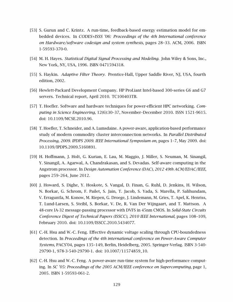
[53] S. Gurun and C. Krintz. A run-time, feedback-based energy estimation model for em-
bedded devices. In CODES+ISSS ’06: Proceedings of the 4th International conference
on Hardware/software codesign and system synthesis, pages 28–33. ACM, 2006. ISBN
1-59593-370-0.
[54] M. H. Hayes. Statistical Digital Signal Processing and Modeling. John Wiley & Sons, Inc.,
New York, NY, USA, 1996. ISBN 0471594318.
[55] S. Haykin. Adaptive Filter Theory. Prentice-Hall, Upper Saddle River, NJ, USA, fourth
edition, 2002.
[56] Hewlett-Packard Development Company. HP ProLiant Intel-based 300-series G6 and G7
servers. Technical report, April 2010. TC100403TB.
[57] T. Hoefler. Software and hardware techniques for power-efficient HPC networking. Com-
puting in Science Engineering, 12(6):30–37, November–December 2010. ISSN 1521-9615.
doi: 10.1109/MCSE.2010.96.
[58] T. Hoefler, T. Schneider, and A. Lumsdaine. A power-aware, application-based performance
study of modern commodity cluster interconnection networks. In Parallel Distributed
Processing, 2009. IPDPS 2009. IEEE International Symposium on, pages 1–7, May 2009. doi:
10.1109/IPDPS.2009.5160891.
[59] H. Hoffmann, J. Holt, G. Kurian, E. Lau, M. Maggio, J. Miller, S. Neuman, M. Sinangil,
Y. Sinangil, A. Agarwal, A. Chandrakasan, and S. Devadas. Self-aware computing in the
Angstrom processor. In Design Automation Conference (DAC), 2012 49th ACM/EDAC/IEEE,
pages 259–264, June 2012.
[60] J. Howard, S. Dighe, Y. Hoskote, S. Vangal, D. Finan, G. Ruhl, D. Jenkins, H. Wilson,
N. Borkar, G. Schrom, F. Pailet, S. Jain, T. Jacob, S. Yada, S. Marella, P. Salihundam,
V. Erraguntla, M. Konow, M. Riepen, G. Droege, J. Lindemann, M. Gries, T. Apel, K. Henriss,
T. Lund-Larsen, S. Steibl, S. Borkar, V. De, R. Van Der Wijngaart, and T. Mattson. A
48-core IA-32 message-passing processor with DVFS in 45nm CMOS. In Solid-State Circuits
Conference Digest of Technical Papers (ISSCC), 2010 IEEE International, pages 108–109,
February 2010. doi: 10.1109/ISSCC.2010.5434077.
[61] C.-H. Hsu and W.-C. Feng. Effective dynamic voltage scaling through CPU-boundedness
detection. In Proceedings of the 4th international conference on Power-Aware Computer
Systems, PACS’04, pages 135–149, Berlin, Heidelberg, 2005. Springer-Verlag. ISBN 3-540-
29790-1, 978-3-540-29790-1. doi: 10.1007/11574859_10.
[62] C.-H. Hsu and W.-C. Feng. A power-aware run-time system for high-performance comput-
ing. In SC ’05: Proceedings of the 2005 ACM/IEEE conference on Supercomputing, page 1,
2005. ISBN 1-59593-061-2.
129

[63] S. Huang and W. Feng. Energy-efficient cluster computing via accurate workload charac-
terization. In Proceedings of the 2009 9th IEEE/ACM International Symposium on Cluster
Computing and the Grid, CCGRID ’09, pages 68–75, Washington, DC, USA, 2009. IEEE
Computer Society. ISBN 978-0-7695-3622-4. doi: 10.1109/CCGRID.2009.88.
[64] IBM PowerExecutive. http://www-03.ibm.com/systems/management/director/
about/director52/extensions/powerexec.html.
[65] InfiniBand Trade Association. http://www.infinibandta.com.
[66] Intel Corporation. http://www.intel.com.
[67] Intel Corporation. Intel Xeon processor E7 family uncore performance monitoring pro-
gramming guide. Technical report, April 2011. Reference Number: 325294-001.
[68] C. Isci. Workload Adaptive Power Management with Live Phase Monitoring and Prediction.
PhD thesis, Princeton University, September 2007.
[69] C. Isci and M. Martonosi. Detecting recurrent phase behavior under real-system variability.
In Workload Characterization Symposium, 2005. Proceedings of the IEEE International,
pages 13–23, October 2005.
[70] C. Isci and M. Martonosi. Runtime power monitoring in high-end processors: Methodology
and empirical data. In MICRO 36: Proceedings of the 36th annual IEEE/ACM International
Symposium on Microarchitecture, page 93. IEEE Computer Society, 2003. ISBN 0-7695-
2043-X.
[71] C. Isci, G. Contreras, and M. Martonosi. Live, runtime phase monitoring and prediction
on real systems with application to dynamic power management. In Proceedings of the
39th Annual IEEE/ACM International Symposium on Microarchitecture, MICRO 39, pages
359–370, Washington, DC, USA, 2006. IEEE Computer Society. ISBN 0-7695-2732-9. doi:
10.1109/MICRO.2006.30.
[72] C. Isci, J. Hanson, I. Whalley, M. Steinder, and J. Kephart. Runtime demand estimation
for effective dynamic resource management. In Network Operations and Management
Symposium (NOMS), 2010 IEEE, pages 381–388, April 2010. doi: 10.1109/NOMS.2010.
5488495.
[73] A. Jain, E. Y. Chang, and Y.-F. Wang. Adaptive stream resource management using Kalman
filters. In SIGMOD ’04: Proceedings of the 2004 ACM SIGMOD international conference on
Management of data, pages 11–22. ACM, 2004. ISBN 1-58113-859-8.
[74] V. Jimenez, R. Gioiosa, F. Cazorla, M. Valero, E. Kursun, C. Isci, A. Buyuktosunoglu, and
P. Bose. Energy-aware accounting and billing in large-scale computing facilities. Micro,
IEEE, 31(3):60–71, May–June 2011. ISSN 0272-1732. doi: 10.1109/MM.2011.35.
130

[75] H. Jin, M. Frumkin, , and J. Yan. The OpenMP implementation of NAS parallel benchmarks
and its performance. Technical report, NAS System Division, NASA Ames Research Center,
October 1999. NAS Technical Report NAS-99-011.
[76] R. Joseph and M. Martonosi. Run-time power estimation in high performance micropro-
cessors. In ISLPED ’01: Proceedings of the 2001 international symposium on Low power
electronics and design, pages 135–140. ACM, 2001. ISBN 1-58113-371-5.
[77] R. Kalla, B. Sinharoy, and J. Tendler. IBM Power5 chip: a dual-core multithreaded processor.
Micro, IEEE, 24(2):40–47, March–April 2004. ISSN 0272-1732. doi: 10.1109/MM.2004.
1289290.
[78] N. Kappiah, V. W. Freeh, and D. K. Lowenthal. Just in time dynamic voltage scaling:
Exploiting inter-node slack to save energy in MPI programs. In SC ’05: Proceedings of the
2005 ACM/IEEE, page 33. IEEE Computer Society, 2005. ISBN 1-59593-061-2.
[79] D. Kerbyson, A. Vishnu, and K. Barker. Energy templates: Exploiting application informa-
tion to save energy. In Cluster Computing (CLUSTER), 2011 IEEE International Conference
on, pages 225–233, September 2011. doi: 10.1109/CLUSTER.2011.33.
[80] Y. Kim, S. Park, Y. Cho, and N. Chang. System-level online power estimation using an
on-chip bus performance monitoring unit. Computer-Aided Design of Integrated Circuits
and Systems, IEEE Transactions on, 30(11):1585–1598, November 2011. ISSN 0278-0070.
doi: 10.1109/TCAD.2011.2160349.
[81] P. Kongetira, K. Aingaran, and K. Olukotun. Niagara: a 32-way multithreaded SPARC
processor. Micro, IEEE, 25(2):21–29, March–April 2005. ISSN 0272-1732. doi: 10.1109/
MM.2005.35.
[82] B. C. Lee and D. M. Brooks. Accurate and efficient regression modeling for microar-
chitectural performance and power prediction. In 12th International Conference on
Architectural support for programming languages and operating systems, pages 185–194.
ACM, 2006. ISBN 1-59593-451-0.
[83] S.-J. Lee, H.-K. Lee, and P.-C. Yew. Runtime performance projection model for dynamic
power management. In Advances in Computer Systems Architecture, volume 4697 of
Lecture Notes in Computer Science, pages 186–197. Springer Berlin / Heidelberg, 2007.
ISBN 978-3-540-74308-8.
[84] A. Lewis, S. Ghosh, and N.-F. Tzeng. Run-time energy consumption estimation based
on workload in server systems. In Proceedings of the 2008 conference on Power aware
computing and systems, HotPower’08, pages 4–4, Berkeley, CA, USA, 2008. USENIX Associ-
ation.
131

[85] A. Lewis, J. Simon, and N.-F. Tzeng. Chaotic attractor prediction for server run-time
energy consumption. In Proceedings of the 2010 international conference on Power aware
computing and systems, HotPower’10, pages 1–16, Berkeley, CA, USA, 2010. USENIX
Association.
[86] D. Li. Scalable and Energy Efficient Execution Methods for Multicore Systems. PhD thesis,
Virginia Polytechnic Institute and State University, January 2011.
[87] D. Li, B. de Supinski, M. Schulz, D. Nikolopoulos, and K. Cameron. Strategies for energy
efficient resource management of hybrid programming models. Parallel and Distributed
Systems, IEEE Transactions on, PP(99):1, 2012. ISSN 1045-9219. doi: 10.1109/TPDS.2012.
95.
[88] T. Li and L. K. John. Run-time modeling and estimation of operating system power
consumption. SIGMETRICS Perform. Eval. Rev., 31(1):160–171, 2003. ISSN 0163-5999.
[89] M. Y. Lim, V. W. Freeh, and D. K. Lowenthal. Adaptive, transparent CPU scaling algorithms
leveraging inter-node MPI communication regions. Parallel Comput., 37(10-11):667–683,
October 2011. ISSN 0167-8191. doi: 10.1016/j.parco.2011.07.001.
[90] Linux performance counters driver - hwpmc. FreeBSD manual 4, http://www.freebsd.
org.
[91] M. Lis, P. Ren, M. H. Cho, K. S. Shim, C. Fletcher, O. Khan, and S. Devadas. Scalable,
accurate multicore simulation in the 1000-core era. In Performance Analysis of Systems
and Software (ISPASS), 2011 IEEE International Symposium on, pages 175–185, April 2011.
doi: 10.1109/ISPASS.2011.5762734.
[92] X. Liu, P. Shenoy, and W. Gong. A time series-based approach for power management in
mobile processors and disks. In Proceedings of the 14th international workshop on Network
and operating systems support for digital audio and video, NOSSDAV ’04, pages 74–79,
New York, NY, USA, 2004. ACM. ISBN 1-58113-801-6. doi: 10.1145/1005847.1005864.
[93] X. Liu, P. Shenoy, and M. Corner. Chameleon: application level power management with
performance isolation. In Proceedings of the 13th annual ACM international conference
on Multimedia, MULTIMEDIA ’05, pages 839–848, New York, NY, USA, 2005. ACM. ISBN
1-59593-044-2. doi: 10.1145/1101149.1101332.
[94] Y. Liu, R. P. Dick, L. Shang, and H. Yang. Accurate temperature-dependent integrated
circuit leakage power estimation is easy. In Proceedings of the conference on Design,
automation and test in Europe, DATE ’07, pages 1526–1531, San Jose, CA, USA, 2007. EDA
Consortium. ISBN 978-3-9810801-2-4.
132

[95] Z. Liu, Y. Chen, C. Bash, A. Wierman, D. Gmach, Z. Wang, M. Marwah, and C. Hyser.
Renewable and cooling aware workload management for sustainable data centers. In
Proceedings of the 12th ACM SIGMETRICS/PERFORMANCE joint international conference
on Measurement and Modeling of Computer Systems, SIGMETRICS ’12, pages 175–186,
New York, NY, USA, 2012. ACM. ISBN 978-1-4503-1097-0. doi: 10.1145/2254756.2254779.
[96] C. Lively, X. Wu, V. Taylor, S. Moore, H.-C. Chang, C.-Y. Su, and K. Cameron. Power-aware
predictive models of hybrid (MPI/OpenMP) scientific applications on multicore systems.
Computer Science - Research and Development, pages 1–9, 2011. ISSN 1865-2034.
[97] P. Mahadevan, S. Banerjee, P. Sharma, A. Shah, and P. Ranganathan. On energy efficiency
for enterprise and data center networks. Communications Magazine, IEEE, 49(8):94–100,
August 2011. ISSN 0163-6804. doi: 10.1109/MCOM.2011.5978421.
[98] J. Manferdelli, N. Govindaraju, and C. Crall. Challenges and opportunities in many-core
computing. Proceedings of the IEEE, 96(5):808–815, May 2008. ISSN 0018-9219. doi:
10.1109/JPROC.2008.917730.
[99] T. G. Mattson, M. Riepen, T. Lehnig, P. Brett, W. Haas, P. Kennedy, J. Howard, S. Vangal,
N. Borkar, G. Ruhl, and S. Dighe. The 48-core SCC processor: the programmer’s view.
In Proceedings of the 2010 ACM/IEEE International Conference for High Performance
Computing, Networking, Storage and Analysis, SC ’10, pages 1–11, Washington, DC, USA,
2010. IEEE Computer Society. ISBN 978-1-4244-7559-9. doi: 10.1109/SC.2010.53.
[100] A. Miyoshi, C. Lefurgy, E. Van Hensbergen, R. Rajamony, and R. Rajkumar. Critical power
slope: understanding the runtime effects of frequency scaling. In Proceedings of the 16th
international conference on Supercomputing, ICS ’02, pages 35–44, New York, NY, USA,
2002. ACM. ISBN 1-58113-483-5. doi: 10.1145/514191.514200.
[101] T. Mudge. Power: a first-class architectural design constraint. Computer, 34(4):52–58, apr
2001. ISSN 0018-9162. doi: 10.1109/2.917539.
[102] Myricom. http://www.myricom.com.
[103] T. Mytkowicz, P. Sweeney, M. Hauswirth, and A. Diwan. Time interpolation: So many
metrics, so few registers. In Microarchitecture, 2007. MICRO 2007. 40th Annual IEEE/ACM
International Symposium on, pages 286–300, December 2007. doi: 10.1109/MICRO.2007.
27.
[104] S. Naffziger, B. Stackhouse, T. Grutkowski, D. Josephson, J. Desai, E. Alon, and M. Horowitz.
The implementation of a 2-core, multi-threaded Itanium family processor. Solid-State
Circuits, IEEE Journal of, 41(1):197–209, January 2006. ISSN 0018-9200. doi: 10.1109/
JSSC.2005.859894.
133

[105] R. Nathuji, K. Schwan, A. Somani, and Y. Joshi. VPM Tokens: virtual machine-aware
power budgeting in datacenters. Cluster Computing, 12:189–203, 2009. ISSN 1386-7857.
10.1007/s10586-009-0077-z.
[106] B. Nayfeh and K. Olukotun. A single-chip multiprocessor. Computer, 30(9):79–85, Septem-
ber 1997. ISSN 0018-9162. doi: 10.1109/2.612253.
[107] K. Olukotun and L. Hammond. The future of microprocessors. Queue, 3(7):26–29,
September 2005. ISSN 1542-7730. doi: 10.1145/1095408.1095418.
[108] M. Pettersson. Linux performance counters driver. http://user.it.uu.se/~mikpe/
linux/perfctr.
[109] Y. Qiao, J. Skicewicz, and P. Dinda. An empirical study of the multiscale predictability
of network traffic. In Proceedings of the 13th IEEE International Symposium on High
Performance Distributed Computing, HPDC ’04, pages 66–76, Washington, DC, USA, 2004.
IEEE Computer Society. ISBN 0-7803-2175-4. doi: 10.1109/HPDC.2004.3.
[110] A. Qureshi, R. Weber, H. Balakrishnan, J. Guttag, and B. Maggs. Cutting the electric bill for
internet-scale systems. SIGCOMM Comput. Commun. Rev., 39(4):123–134, August 2009.
ISSN 0146-4833. doi: 10.1145/1594977.1592584.
[111] K. Rajamani, H. Hanson, J. C. Rubio, S. Ghiasi, and F. L. Rawson. Online power and
performance estimation for dynamic power management. Technical report, International
Business Machines (IBM) Corporation, 2006.
[112] M. Rashti and A. Afsahi. 10-Gigabit iWARP Ethernet: Comparative performance analysis
with InfiniBand and Myrinet-10G. In Parallel and Distributed Processing Symposium, 2007.
IPDPS 2007. IEEE International, pages 1–8, March 2007. doi: 10.1109/IPDPS.2007.370480.
[113] B. Rountree, D. Lowenthal, M. Schulz, and B. de Supinski. Practical performance prediction
under dynamic voltage frequency scaling. In Green Computing Conference and Workshops
(IGCC), 2011 International, pages 1–8, July 2011. doi: 10.1109/IGCC.2011.6008553.
[114] L. Rountree. Theory and Practice of Dynamic Voltage/Frequency Scaling in the High
Performance Computing Environment. PhD thesis, The University of Arizona, 2010.
[115] S. Saini, H. Jin, R. Hood, D. Barker, P. Mehrotra, and R. Biswas. The impact of Hyper-
Threading on processor resource utilization in production applications. In High Perfor-
mance Computing (HiPC), 2011 18th International Conference on, pages 1–10, December
2011. doi: 10.1109/HiPC.2011.6152743.
[116] V. Salapura, K. Ganesan, A. Gara, M. Gschwind, J. Sexton, and R. Walkup. Next-generation
performance counters: Towards monitoring over thousand concurrent events. In Perfor-
mance Analysis of Systems and software, 2008. ISPASS 2008. IEEE International Symposium
on, pages 139–146, April 2008. doi: 10.1109/ISPASS.2008.4510746.
134

[117] R. Sarikaya and A. Buyuktosunoglu. A unified prediction method for predicting program
behavior. Computers, IEEE Transactions on, 59(2):272–282, February 2010. ISSN 0018-9340.
doi: 10.1109/TC.2009.122.
[118] R. Sarikaya, C. Isci, and A. Buyuktosunoglu. Runtime workload behavior prediction using
statistical metric modeling with application to dynamic power management. In Workload
Characterization (IISWC), 2010 IEEE International Symposium on, pages 1–10, December
2010. doi: 10.1109/IISWC.2010.5650339.
[119] H. Sasaki, Y. Ikeda, M. Kondo, and H. Nakamura. An intra-task DVFS technique based on
statistical analysis of hardware events. In Proceedings of the 4th international conference
on Computing frontiers, CF ’07, pages 123–130, New York, NY, USA, 2007. ACM. ISBN
978-1-59593-683-7. doi: 10.1145/1242531.1242551.
[120] A. Shye, M. Iyer, V. J. Reddi, and D. A. Connors. Code coverage testing using hardware
performance monitoring support. In Proceedings of the sixth international symposium on
Automated analysis-driven debugging, AADEBUG’05, pages 159–163, New York, NY, USA,
2005. ACM. ISBN 1-59593-050-7. doi: 10.1145/1085130.1085151.
[121] K. Skadron, M. Stan, W. Huang, S. Velusamy, K. Sankaranarayanan, and D. Tarjan.
Temperature-aware microarchitecture. In Computer Architecture, 2003. Proceedings.
30th Annual International Symposium on, pages 2–13, June 2003. doi: 10.1109/ISCA.
2003.1206984.
[122] W. Smith. Prediction services for distributed computing. In Parallel and Distributed
Processing Symposium, 2007. IPDPS 2007. IEEE International, pages 1–10, March 2007.
doi: 10.1109/IPDPS.2007.370276.
[123] D. C. Snowdon, S. M. Petters, and G. Heiser. Accurate on-line prediction of processor
and memory energy usage under voltage scaling. In Proceedings of the 7th ACM & IEEE
International Conference on Embedded software, pages 84–93, 2007. ISBN 978-1-59593-
825-1.
[124] L. Spracklen and S. Abraham. Chip multithreading: opportunities and challenges. In
High-Performance Computer Architecture, 2005. HPCA-11. 11th International Symposium
on, pages 248–252, February 2005. doi: 10.1109/HPCA.2005.10.
[125] B. Sprunt. The basics of performance-monitoring hardware. Micro, IEEE, 22(4):64–71,
July–August 2002. ISSN 0272-1732. doi: 10.1109/MM.2002.1028477.
[126] J. Srinivasan, S. V. Adve, P. Bose, J. Rivers, and C.-K. Hu. RAMP: A model for reliability
aware microprocessor design. Technical report, IBM Research Division, Thomas J. Watson
Research Center, Yorktown Heights, NY 10598, December 2003. IBM Research Report,
Computer Science, RC23048 (W0312-122).
135

[127] D. Talla, L. John, and D. Burger. Bottlenecks in multimedia processing with SIMD style
extensions and architectural enhancements. Computers, IEEE Transactions on, 52(8):
1015–1031, August 2003. ISSN 0018-9340. doi: 10.1109/TC.2003.1223637.
[128] P.-N. Tan, M. Steinbach, and V. Kumar. Introduction to Data Mining, (First Edition). Addison-
Wesley Longman Publishing Co., Inc., Boston, MA, USA, 2005. ISBN 0321321367.
[129] The Green500 List. http://www.green500.org.
[130] The Message Passing Interface Forum. http://www.mpi-forum.org.
[131] The NAS Parallel Benchmarks. http://www.nas.nasa.gov.
[132] The OpenMP API. http://www.openmp.org.
[133] The Top500 Supercomputing Site. http://www.top500.org.
[134] D. M. Tullsen, S. J. Eggers, and H. M. Levy. Simultaneous multithreading: maximizing
on-chip parallelism. In 25 years of the international symposia on Computer architecture
(selected papers), ISCA ’98, pages 533–544, New York, NY, USA, 1998. ACM. ISBN 1-58113-
058-9. doi: 10.1145/285930.286011.
[135] T. Ungerer, B. Robic, and J. Šilc. A survey of processors with explicit multithreading. ACM
Comput. Surv., 35(1):29–63, March 2003. ISSN 0360-0300. doi: 10.1145/641865.641867.
[136] A. Vishnu, S. Song, A. Marquez, K. Barker, D. Kerbyson, K. Cameron, and P. Balaji.
Designing energy efficient communication runtime systems for data centric programming
models. In Green Computing and Communications (GreenCom), 2010 IEEE/ACM Int’l
Conference on Int’l Conference on Cyber, Physical and Social Computing (CPSCom), pages
229–236, December 2010. doi: 10.1109/GreenCom-CPSCom.2010.133.
[137] A. Vishnu, S. Song, A. Marquez, K. Barker, D. Kerbyson, K. Cameron, and P. Balaji.
Designing energy efficient communication runtime systems: a view from PGAS models.
The Journal of Supercomputing, pages 1–19, 2011. ISSN 0920-8542. 10.1007/s11227-011-
0699-9.
[138] Z. Wang, X. Zhu, and S. Singhal. Utilization and SLO-based control for dynamic sizing of
resource partitions. In IFIP/IEEE Distributed Systems: Operations and Management, pages
24–26, 2005.
[139] M. Weiser, B. Welch, A. Demers, and S. Shenker. Scheduling for reduced CPU energy. In Pro-
ceedings of the 1st USENIX conference on Operating Systems Design and Implementation,
OSDI ’94, Berkeley, CA, USA, 1994. USENIX Association.
[140] G. Welch and G. Bishop. An introduction to the Kalman filter. Technical report, University
of North Carolina, Chapel Hill, NC, USA, 1995.
136

[141] R. Wolski. Forecasting network performance to support dynamic scheduling using the
network weather service. In High Performance Distributed Computing, 1997. Proceedings.
The Sixth IEEE International Symposium on, pages 316–325, August 1997. doi: 10.1109/
HPDC.1997.626437.
[142] R. Wolski, N. Spring, and J. Hayes. Predicting the CPU availability of time-shared Unix
systems on the computational grid. In Proceedings of the 8th IEEE International Symposium
on High Performance Distributed Computing, HPDC ’99, page 12, Washington, DC, USA,
1999. IEEE Computer Society. ISBN 0-7695-0287-3.
[143] R. Wolski, N. T. Spring, and J. Hayes. The network weather service: a distributed resource
performance forecasting service for metacomputing. Future Generation Computing
Systems, 15(5–6):757–768, October 1999. ISSN 0167-739X. doi: 10.1016/S0167-739X(99)
00025-4.
[144] Y. Wu, Y. Yuan, G. Yang, and W. Zheng. Load prediction using hybrid model for com-
putational grid. In Proceedings of the 8th IEEE/ACM International Conference on Grid
Computing, GRID ’07, pages 235–242, Washington, DC, USA, 2007. IEEE Computer Society.
ISBN 978-1-4244-1559-5. doi: 10.1109/GRID.2007.4354138.
[145] W. A. Wulf and S. A. McKee. Hitting the memory wall: implications of the obvious.
SIGARCH Comput. Archit. News, 23(1):20–24, March 1995. ISSN 0163-5964. doi: 10.1145/
216585.216588.
[146] X. X. Xin and T. T. Tiow. IPC-driven energy reduction for low-power design. In Circuits and
Systems, 2006. ISCAS 2006. Proceedings. 2006 IEEE International Symposium on, page 4,
May 2006. doi: 10.1109/ISCAS.2006.1693417.
[147] W. Xu, X. Zhu, S. Singhal, and Z. Wang. Predictive control for dynamic resource allocation
in enterprise data centers. In Network Operations and Management Symposium, pages
115–126, 3-7 2006.
[148] L. Yang, I. Foster, and J. Schopf. Homeostatic and tendency-based CPU load predictions. In
Parallel and Distributed Processing Symposium, 2003. Proceedings. International, page 9,
April 2003. doi: 10.1109/IPDPS.2003.1213129.
[149] L. Yang, J. M. Schopf, and I. Foster. Conservative scheduling: Using predicted variance
to improve scheduling decisions in dynamic environments. In Proceedings of the 2003
ACM/IEEE conference on Supercomputing, SC ’03, page 31, New York, NY, USA, 2003. ACM.
ISBN 1-58113-695-1. doi: 10.1145/1048935.1050182.
[150] R. Zamani and A. Afsahi. Performance monitoring counter-based power estimation under
DVFS. Journal Publication (in preparation), 2012.
137

[151] R. Zamani and A. Afsahi. Adaptive estimation and prediction of power and performance
in high performance computing. Computer Science - Research and Development, 25:
177–186, 2010. ISSN 1865-2034.
[152] R. Zamani and A. Afsahi. A study of hardware performance monitoring counter selection
in power modeling of computing systems. In Green Computing Conference (IGCC), 2012
International, pages 1–10, June 2012. doi: 10.1109/IGCC.2012.6322289.
[153] R. Zamani, A. Afsahi, Y. Qian, and C. Hamacher. A feasibility analysis of power-awareness
and energy minimization in modern interconnects for high-performance computing. In
Proceedings of the IEEE International Conference on Cluster Computing, pages 118–128,
2007. ISBN 978-1-4244-1387-4.
[154] R. Zamani, A. Afsahi, R. P. Anderson, and M. Mallin. Run-time predictive modeling
of performance monitoring counters and power consumption under DVFS. Journal
Publication (in preparation), 2012.
[155] L. Zhang, B. Tiwana, R. Dick, Z. Qian, Z. Mao, Z. Wang, and L. Yang. Accurate online
power estimation and automatic battery behavior based power model generation for
smartphones. In Hardware/Software Codesign and System Synthesis (CODES+ISSS), 2010
IEEE/ACM/IFIP International Conference on, pages 105–114, October 2010.
[156] X. Zhu, M. Uysal, Z. Wang, S. Singhal, A. Merchant, P. Padala, and K. Shin. What does
control theory bring to systems research? SIGOPS Oper. Syst. Rev., 43(1):62–69, 2009.
ISSN 0163-5980.
138


