
Paper: ASAT-14-017-GU
14th
International Conference on
AEROSPACE SCIENCES & AVIATION TECHNOLOGY,
ASAT - 14 – May 24 - 26, 2011, Email: [email protected]
Military Technical College, Kobry Elkobbah, Cairo, Egypt
Tel: +(202) 24025292 –24036138, Fax: +(202) 22621908
1
Robust CLOS Guidance and Control:
Part-1: System Modeling and Uncertainty Evaluation
A.N. Oda*, G.A. El-Sheikh
†, Y.Z. El-Halwagy
* and M. Al-Ashry
*
Abstract: The great developments in applied mathematics and computational capabilities facilitate
the design and implementation of robust control. In addition, the huge developments in
nanotechnology and its availability in civilian level with less cost, size and weight attract many of the
researchers allover the world towards embedded systems especially the embedded flight control.
Among the real applications are the guided missiles especially the antitank guided missile systems
which are commanded to the line of sight (CLOS) against ground and short range targets. The present
work is concerned with improving the performance of an antitank guided missile system belonging to
the first generation via robust synthesis of autopilot and guidance systems. The design and analysis
necessitates somehow accurate model with different uncertainties (objective of Part-1 of the paper) for
the system, a robust autopilot design (objective of Part-2 of the paper) and implementation via
hardware in the loop (HIL) simulation (objective of Part-3 of the paper).
This part of the paper is devoted to the derivation of the system equations of motion clarifying
different sources of uncertainty including thrust aging, anomalies in aerodynamic coefficients and
derivatives and wind velocity effects. The solution of these equations is described in the form of
modules programmed within the C++ and MATLAB environments to form the baseline for
subsequent design and analysis. The simulation is conducted with different engagement scenarios and
different levels of uncertainty in thrust, aerodynamics and wind velocity. The simulation results are
validated against reference data and verified for performance requirements including the time of flight,
miss distance, control currents, normal acceleration and angles of attack. This investigation clarified
the closeness of the designed model performance to the reference and its appropriateness for autopilot
design and HIL simulation in the next parts of the paper.
Keywords: Command Guidance Systems, CLOS, Robust Control, Uncertainties
Nomenclature X1, Y1, and Z1 Vectors components along the board reference axes
Xg,Yg, and Zg Vectors components along the ground reference axes
X, Y, and Z Vectors components along the velocity reference axes
Tbg Transformation matrix from board to ground reference axes
Tvg Transformation matrix from velocity to ground reference axes
Tbg Transformation matrix from board to ground reference axes
jp and jy Thrust jetivator angles in pitch and yaw planes
F,, FF TZTYTX and 11 1
Thrust forces along the board reference axes
AXF , AYF ,and AZF Drag, lateral, and lift forces along the velocity axes
S Characteristic area
Q Dynamic pressure given by q = 0.5 (vm)2 [Kg/m/sec2]
* Egyptian Armed Forces, Egypt
† Professor, , [email protected], Tel. 02,01002682402
Paper: ASAT-14-017-GU
2
Air density [kg/m3]
VM Missile velocity
Cx , Cy , and Cz Dimension-less aerodynamic coefficients
ms Instantaneous total missile mass
g Vector of gravity acceleration
mo Initial missile mass and
msec Burnt quantity of fuel or propellant per second
M Mach number and given by M=vm/va
Va Sound velocity at missile position
Tl Perpendicular distance between the missile C.G. and the action-point of lateral thrust
forces
TXl Perpendicular distance between longitudinal axis and thrust force line
zyx lll ,, Characteristic linear dimensions of missile
1xm , 1ym , and
1zm Dimensionless aerodynamic coefficients
1 1 1,x y zand Airframe-turn rates along board coordinate axes
J Acceleration of missile
Angular velocity of VCS with respect to GCS
IXX, IYY, and IZZ Moments of inertia components along the BCS
Angle of attack [angle of incidence] [Degree]
Sideslip angle [angle of drift] [Degree]
U, V, and W Velocities Along board coordinate axis
Ud, Vd, and Wd Derivative of velocities along board coordinate axis
gx, gY, and gZ Gravity acceleration along board coordinate axis
T and T Elevation and azimuth angles of target
M and M Elevation and azimuth angles of missile
Δ and Δ LOS angular error
Rm and Rt Missile and target range
p Pitch demand
s Angle between missile and LOS in yaw plane
1, 1 LOS angular errors for the two planes expressed in meters
Eo Temperature compensation term
θc Crest angle
θs Angle between sight forward axis and LOS in pitch plane
A Micro ampere
N Newton
Abbreviations ACLOS Automatic commanded to line of sight
ADC Aero Dynamic Coefficients
ATGM Anti Tank Guided Missile
BCS Board coordinate system
CBR Transformation matrix from board to reference coordinate System
C.G. Missile center of gravity
CLOS Commanded to line of sight
C.P. Center of pressure
CRB Transformation matrix from reference to board Coordinate System
E-D Electronic Driver
FOR-MON Force-Moment
FOV Field of view
FSM Flight simulation model
GCS Ground coordinate system

Paper: ASAT-14-017-GU
3
HIL hardware in the loop
I/P Input
IR Infra-Red
LOS Line of sight
MCLOS Manual command to line of sight
PEC Programmer electronic controller
PD Proportional Derivative
PI Proportional Integral
PID Proportional Integral Derivative
RK4 Runge- Kutta 4
SACLOS Semi-Automatic command to line of sight
6-DOF Six degrees of freedom
TF Transfer function
TVC Thrust vector control
VCS Velocity coordinate system
1. Introduction Antitank guided missiles (ATGM) are command guidance systems launched against tanks and
armored vehicles. These missiles are classified into three generations; the first generation in which
both the target and missile are manually tracked using optical telescopes. The second generation in
which the target is manually tracked using optical telescopes while the missile is automatically tracked
by including an infrared sensor in the launcher with the telescope to detect the IR radiation from a
source strapped on the rear part of the missile. Then the motion parameters are transferred
automatically to signals applied to the guidance unit. The third generation is characterized by manual
or automatic target tracking through optical telescopes, TV, laser or radio devices and the missile is
automatically tracked as in the second generation. However, the guidance commands in this
generation are transmitted to the missile through a remote link instead of wires. Note that this
generation could be of the semi-active homing guidance in which guidance commands are generated
onboard.In a command guidance system an operator or a computer at the control point solves the
mission of interception on the basis of obtained coordinates for both target and missile and forms the
command, according to the utilized or specified guidance method, for the control system on the
missile, which changes its spatial position. A telescope or TV camera based on the parent platform
tracks the target and the missile to yield tracking data to be sent to the system guidance computer. The
guidance computer compares the two sets of tracking data (for target and missile) and extracts the
appropriate corrections (guidance commands) according to the employed guidance method. Then, it
applies these commands to the missile through a wire link during its flight. That is, the guidance of a
missile is carried out either totally by the operator or partially by the interaction between human and
electronic circuits constituting the guidance unit. According to these features, the antitank command
guidance systems are divided into three main sub groups: manual command to line of sight (MCLOS),
semi-automatic CLOS (SACLOS) and automatic CLOS (ACLOS) [1,2,7,8,15,16]. However, these
literature did not manipulate the different sources of uncertainty corrupting the performance
of such systems; one of the objectives in this work.
Using a command link imposes some limitations upon the guidance system such as data rate
of transfer, loop delay and jamming. In addition, the ever-increasing role of armored forces in
modern combat directs the designers and manufacturers towards increasing the tank
capabilities. These capabilities include tank power and design improvement, armor
production, maneuverability of tanks and jamming. These ever-increasing developments of
tanks’ capabilities necessitate the design of accurate guidance and control system for an
antitank missile in presence of disturbance, measurement noise, and un-modelled dynamics.
In addition, the underlying system has different sources of uncertainty including the forward
loop gains, the thrust values due to aging, aerodynamic coefficients and derivatives due to
lack of accurate wind tunnel tests, and expected wind velocities. These uncertainties lead, e.g.,
to anomalies in the missile flight behavior just after launch and yield to bring the missile
Paper: ASAT-14-017-GU
4
down at lower values of thrust such that it impacts the ground. To overcome uncertainties and
achieve the mission, this paper is devoted to derive an adequate nonlinear mathematical
model representing the dynamical behaviour of the underlying missile for different flight
phases and with uncertainties’ quantification.
The evaluation of obtained mathematical model is carried out via simulation which is
indispensable tool in the design and development and where the set of equations are
programmed within MATLAB and C++ environments. The input stimuli are launch
conditions (pitch and yaw angles), target position, target motion and its trajectory
characterization. The outputs are the missile flight data (thrust profile, speed, acceleration,
range, angle of attack, incidence angle, jetivator deflections, flight time, miss distance, etc.)
during the engagement. The obtained six degrees of freedom (6DOF) mathematical model
consists of the equations describing kinematics, dynamics (weight, thrust, aerodynamic
forces), command guidance generation system, instruments, compensation electronics,
autopilot variables and estimates for the different sources of uncertainty. Using these models
it is possible to draw contribution about the reliability of conceptual hardware design and
hence to the requirement for the number of very expensive flight trials. In addition, it enables
questions to be answered that it would not be possible to answer in any other way and
consequently the system performance can be evaluated against futuristic targets [14].
2. Missile Flight Modeling
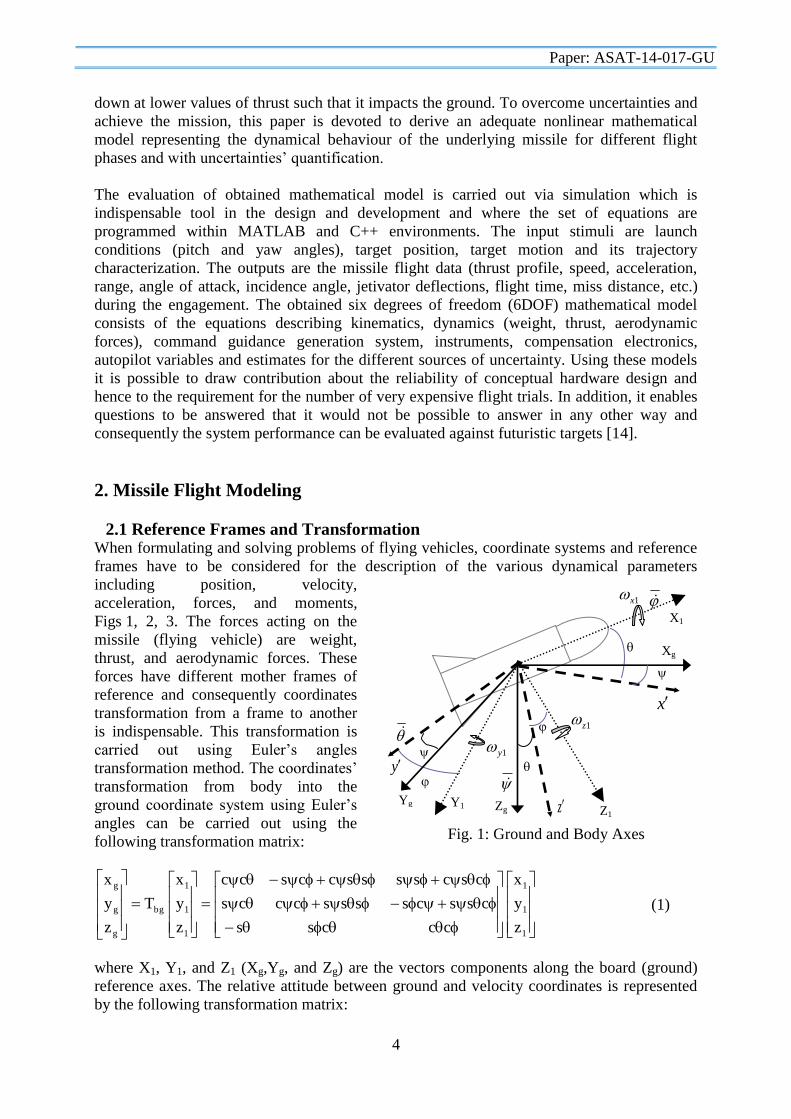
2.1 Reference Frames and Transformation When formulating and solving problems of flying vehicles, coordinate systems and reference
frames have to be considered for the description of the various dynamical parameters
including position, velocity,
acceleration, forces, and moments,
Figs 1, 2, 3. The forces acting on the
missile (flying vehicle) are weight,
thrust, and aerodynamic forces. These
forces have different mother frames of
reference and consequently coordinates
transformation from a frame to another
is indispensable. This transformation is
carried out using Euler’s angles
transformation method. The coordinates’
transformation from body into the
ground coordinate system using Euler’s
angles can be carried out using the
following transformation matrix:
1
1
1
1
1
1
bg
g
g
g
z
y
x
cccss
csscsssscccs
cscssssccscc
z
y
x
T
z
y
x
(1)
where X1, Y1, and Z1 (Xg,Yg, and Zg) are the vectors components along the board (ground)
reference axes. The relative attitude between ground and velocity coordinates is represented
by the following transformation matrix:
1x
Xg
X1
x
1z
Z1 z Zg
1y
Yg
y
Y1
Fig. 1: Ground and Body Axes

Paper: ASAT-14-017-GU
5
z
y
x
cccss
cscssssscccs
cscsscsssccc
z
y
x
T
z
y
x
vg
g
g
g
(2)
where X, Y, and Z (Xg, Yg, and Zg) are the vectors’ components along the velocity (ground)
reference-axes. The coordinates’ transformation from velocity into body coordinates axes can
be carried using the following matrix:
1
1
1
1
1
1
vg
z
y
x
c0s
ssccs
scscc
z
y
x
T
z
y
x
(3)
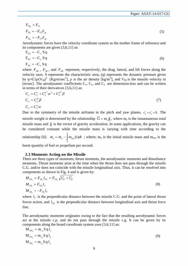
2.2 Acting Forces
The thrust forces that act on the missile are inclined by angles jp and jy in the pitch and yaw
planes [3,6,11] as shown in Fig. 4 and it can be resolved as:
jpTTZ
jyjpTTY
jyjpTTX
FF
FF
FF
sin
sincos
coscos
1
1
1
1
1
1
(4)
The thrust jetivator angles jp and jy are small enough such that Eqn (4) can be simplified as:
1TZF
1TXF
C.G.
MZ1 MY1
It
Z1 Y1
Y1 Z1
X1
1TF
1TYF jy jp
Fig. 4: Thrust forces and moments
X Y
X
Y1
X1
Z1
Z
Y
Z
Fig. 3: Velocity and Body axes
Xg
X
Z
z
x
z
Y
y
Yg
y
x
Zg
Fig. 2: Ground and Velocity Axes
Paper: ASAT-14-017-GU
6
jpTTZ
jyTTY
TTX
FF
FF
FF
1
1
1
1
1
1
(5)
Aerodynamic forces have the velocity coordinate system as the mother frame of reference and
its components are given [3,6,11] as:
q S CF
q S CF
q S CF
zAZ
yAY
xAX
(6)
where AXF , AYF , and AZF represent, respectively, the drag, lateral, and lift forces along the
velocity axes. S represents the characteristic area, (q) represents the dynamic pressure given
by q=0.5(VM)2
[Kg/m/sec2], is the air density [kg/m
3], and VM is the missile velocity in
[m/sec]. The aerodynamic coefficients Cx, Cy, and Cz are dimension-less and can be written
in terms of their derivatives [3,6,11] as:
zz
yy
xxxx
CC
CC
CCCC
22 2
(7)
Due to the symmetry of the missile airframe in the pitch and yaw planes, 0cc zy . The
missile weight is determined by the relationship gmG s , where ms is the instantaneous total
missile mass and g is the vector of gravity acceleration. In some applications, the gravity can
be considered constant while the missile mass is varying with time according to the
relationship [6]:
t
os dttmmm0
sec )( ; where; mo is the initial missile mass and msec is the
burnt quantity of fuel or propellant per second.
2.3 Moments Acting on the Missile There are three types of moments; thrust moments, the aerodynamic moments and disturbance
moments. Thrust moments arise at the time when the thrust does not pass through the missile
C.G. and/or does not coincide with the missile longitudinal axis. Thus, it can be resolved into
components as shown in Fig. 4 and is given by:
TTYTZ
TTZTY
TZTYTXTXTXTX
lFM
lFM
llFlFM
11
11
111
22
(8)
where Tl is the perpendicular distance between the missile C.G. and the point of lateral thrust
forces action, and TXl is the perpendicular distance between longitudinal axis and thrust force
line.
The aerodynamic moments originates owing to the fact that the resulting aerodynamic forces
act at the missile c.p. and do not pass through the missile c.g. It can be given by its
components along the board coordinate system axes [3,6,11] as:
zzAZ
yyAY
xxAX
l q SmM
l q SmM
l q SmM
11
11
11
(9)
Paper: ASAT-14-017-GU
7
where: zyx lll ,, are the Characteristic linear dimensions of missile, S is the characteristic area
of missile, and 1xm ,
1ym , and 1z
m are dimensionless aerodynamic coefficients. These
functions are usually allocated in the form of graphs obtained by experiments in a wind
tunnel. For X-form missile, the aerodynamic moments derivatives are given by [3,6]:
11
1
11
11
1
11
1
1
11
zzzz
yyyy
xxx
mmm
mmm
mm
z
y
x
(10)
where 1 1 1,x y zand are the airframe-turn rates along board coordinate axes as shown in
Fig. 3.
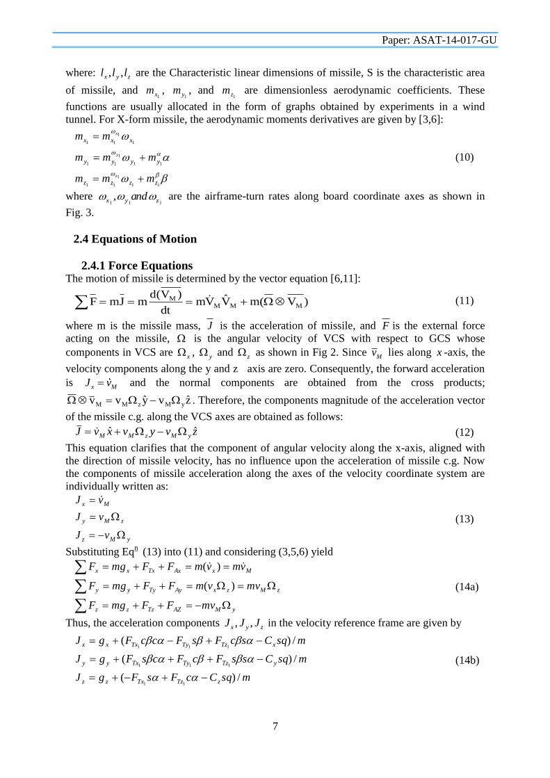
2.4 Equations of Motion
2.4.1 Force Equations The motion of missile is determined by the vector equation [6,11]:
)V(mVVmdt
)V(dmJmF MMM
M (11)
where m is the missile mass, J is the acceleration of missile, and F is the external force
acting on the missile, is the angular velocity of VCS with respect to GCS whose
components in VCS are x , y and z as shown in Fig 2. Since Mv lies along x -axis, the
velocity components along the y and z axis are zero. Consequently, the forward acceleration
is x MJ v and the normal components are obtained from the cross products;
zvyvv yMzMM . Therefore, the components magnitude of the acceleration vector
of the missile c.g. along the VCS axes are obtained as follows:
zvyvxvJ yMzMMˆˆ (12)
This equation clarifies that the component of angular velocity along the x-axis, aligned with
the direction of missile velocity, has no influence upon the acceleration of missile c.g. Now
the components of missile acceleration along the axes of the velocity coordinate system are
individually written as:
yMz
zMy
Mx
vJ
vJ
vJ
(13)
Substituting Eqn
(13) into (11) and considering (3,5,6) yield
yMAZTzzz
zMzxAyTyyy
MxAxTxxx
mvFFmgF
mvvmFFmgF
vmvmFFmgF
)(
)(
(14a)
Thus, the acceleration components , ,x y zJ J J in the velocity reference frame are given by
msqCcFsFgJ
msqCssFcFcsFgJ
msqCscFsFccFgJ
zTzTxzz
yTzTyTxyy
xTzTyTxxx
/)(
/)(
/)(
11
111
111
(14b)
Paper: ASAT-14-017-GU
8
The thrust force components projected into the velocity coordinate system has the form
1TbvT FTF , whose components are using the transformation matrix Eqn(3) as
cFsFF
ssFcFcsFF
scFsFccFF
TzTxTz
TzTyTxTy
TzTyTxTx
11
111
111
(15)
The acceleration components 111
,, zyx JJJ in the body reference frame are given by JTJ vb1 ,
whose components are using the transformation matrix Eqn(3) as
cJssJscJJ
cJsJJ
sJcsJccJJ
zyxz
yxy
zyxx
1
1
1
(16)
The position of the velocity coordinate system with respect to the reference ground coordinate
system is determined by means of three angles ( , , ). Therefore, the angular velocity
vector ( ) of missile rotation with respect to GCS (earth reference system) is given by its
components in the direction of VCS axes as x , y and z as shown in Fig. 2. These
components can be related to angular rates of Euler’s angles ( , , ) through the direction
cosines [10] and the algebraic manipulation of its elements yields the angular raters of Euler’s
angles as follows:
)sincos(tan
cossincos
sincos
yzx
zy
zy
(17)
The components of gravity along the VCS axes are obtained using the transformation matrix
Eqn(2) as follows:
cgc
sgc
gs
gccsccsssscsc
scssscccsssc
scscc
g
g
g
z
y
x
0
0
From the above discussions, it is clear that the equation describing dynamics of guided
missile c.g. motion can be summarized as:
cossincos
cossincos
KN
v
gKN
m
sqCgv
M
x
xxM
(18)
where
mscFsFccF TzTyTxx /)(111
)(1
11 cFsF
mvn TzTx
M
kkK
)(1
sqCmv
k y
M
nnN
)(1
sqCmv
n z
M
)(1
111 ssFcFcsF
mvk TzTyTx
M
Paper: ASAT-14-017-GU
9
2.4.2 Moment Equations The external moments acting on a body equal to the time rate of change of its moment of
momentum (angular momentum). The time rates of change are all taken with respect to
inertial space and can be expressed as follows [6,11]:
Idt
HdM
)( (19)
where the subscript (I) indicates that the time rate of change of the vector is obtained with
respect to inertial space. Due to symmetry of missile configuration, the products of inertia are
neglected [6,11] and the equations of missile rotation around its c.g. are obtained as follows:
tan)sincos(
cos/)sincos(
sincos
111
11
11
yzx
yz
zy
(20a)
1111
1111
1111
)(
)(
)(
yxxxyyzzzz
xzzzxxyyyy
yzyyzzxxxx
IIIM
IIIM
IIIM
(20b)
where IXX, IYY, and IZZ are moments of inertia components along the board coordinate axes.
The manipulation of Eqn (20b) yields the dynamic equations of missile rotation around its c.g.
as follows [9,11,13]:
zzxyyyxxzzzz
yyzxxxzzyyyy
xxzyzzyyxxxx
IIIIM
IIIIM
IIIIM
/)(/
/)(/
/)(/
1111
1111
1111
(21)
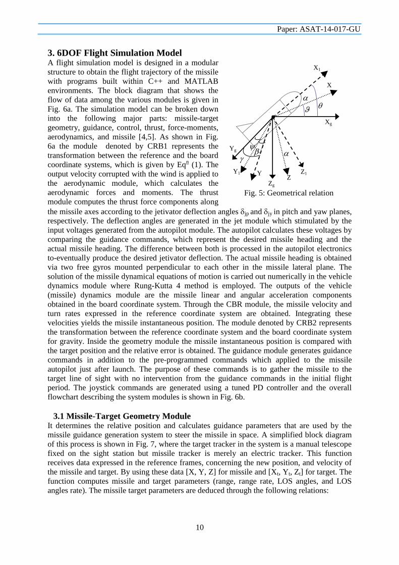
2.4.3 Geometrical Relations The relative attitude between reference frames can be described by considering the Euler’s
angles ( , , ) of VCS with respect to GCS, ( , ) angles of VCS with respect to BCS,
angles ( , , ) between BCS with respect to GCS and combined rotations of reference
frames as shown in Fig. 5; i.e.
ggv
ggb
bv
xTx
xTx
xTx
1
1
(22a)
Manipulating these equations yields gvvbgb TTT , from which only three elements are selected
from the above equations to yield the geometrical relations as follows:
)cos/)cossin((
costansintan
cossin
(22b)
Paper: ASAT-14-017-GU
10
Z1 Z
Xg
X
Yg
Y1 Y
Zg
X1
Fig. 5: Geometrical relation
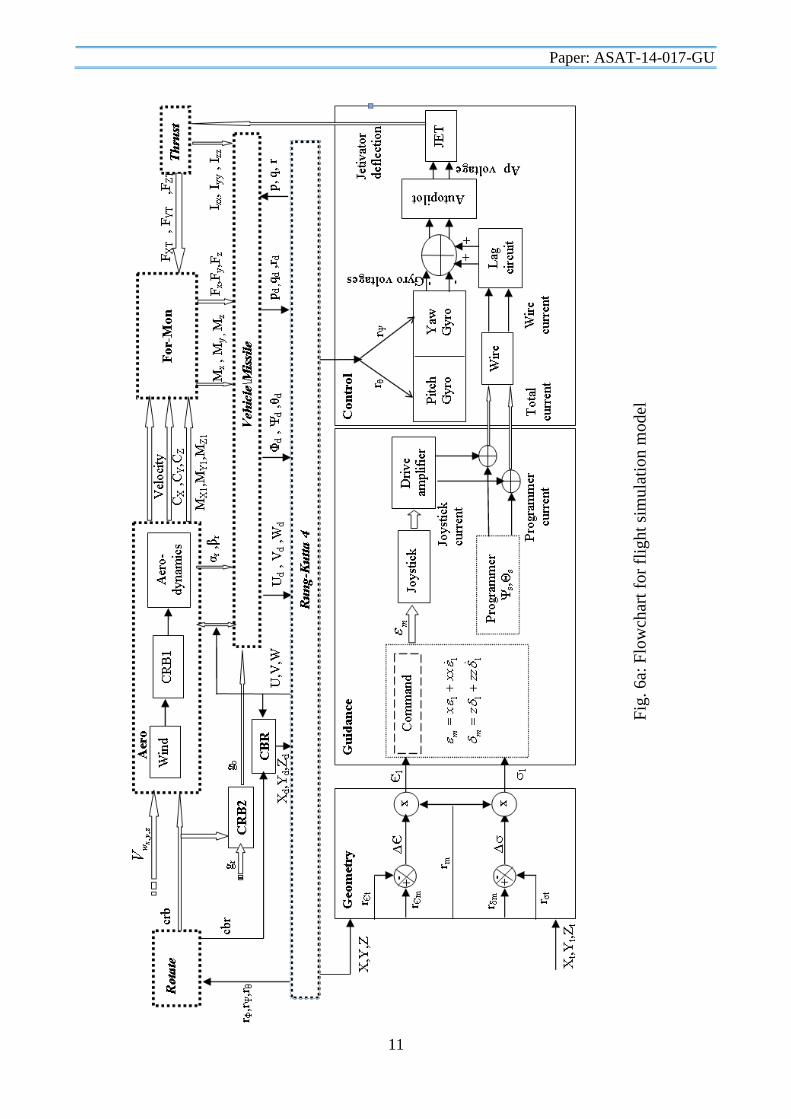
3. 6DOF Flight Simulation Model A flight simulation model is designed in a modular
structure to obtain the flight trajectory of the missile
with programs built within C++ and MATLAB
environments. The block diagram that shows the
flow of data among the various modules is given in
Fig. 6a. The simulation model can be broken down
into the following major parts: missile-target
geometry, guidance, control, thrust, force-moments,
aerodynamics, and missile [4,5]. As shown in Fig.
6a the module denoted by CRB1 represents the
transformation between the reference and the board
coordinate systems, which is given by Eqn (1). The
output velocity corrupted with the wind is applied to
the aerodynamic module, which calculates the
aerodynamic forces and moments. The thrust
module computes the thrust force components along
the missile axes according to the jetivator deflection angles jp and jy in pitch and yaw planes,
respectively. The deflection angles are generated in the jet module which stimulated by the
input voltages generated from the autopilot module. The autopilot calculates these voltages by
comparing the guidance commands, which represent the desired missile heading and the
actual missile heading. The difference between both is processed in the autopilot electronics
to-eventually produce the desired jetivator deflection. The actual missile heading is obtained
via two free gyros mounted perpendicular to each other in the missile lateral plane. The
solution of the missile dynamical equations of motion is carried out numerically in the vehicle
dynamics module where Rung-Kutta 4 method is employed. The outputs of the vehicle
(missile) dynamics module are the missile linear and angular acceleration components
obtained in the board coordinate system. Through the CBR module, the missile velocity and
turn rates expressed in the reference coordinate system are obtained. Integrating these
velocities yields the missile instantaneous position. The module denoted by CRB2 represents
the transformation between the reference coordinate system and the board coordinate system
for gravity. Inside the geometry module the missile instantaneous position is compared with
the target position and the relative error is obtained. The guidance module generates guidance
commands in addition to the pre-programmed commands which applied to the missile
autopilot just after launch. The purpose of these commands is to gather the missile to the
target line of sight with no intervention from the guidance commands in the initial flight
period. The joystick commands are generated using a tuned PD controller and the overall
flowchart describing the system modules is shown in Fig. 6b.
3.1 Missile-Target Geometry Module It determines the relative position and calculates guidance parameters that are used by the
missile guidance generation system to steer the missile in space. A simplified block diagram
of this process is shown in Fig. 7, where the target tracker in the system is a manual telescope
fixed on the sight station but missile tracker is merely an electric tracker. This function
receives data expressed in the reference frames, concerning the new position, and velocity of
the missile and target. By using these data [X, Y, Z] for missile and [Xt, Yt, Zt] for target. The
function computes missile and target parameters (range, range rate, LOS angles, and LOS
angles rate). The missile target parameters are deduced through the following relations:
Paper: ASAT-14-017-GU
11
Fig
. 6
a: F
low
char
t fo
r fl
igh
t si
mu
lati
on
model

Paper: ASAT-14-017-GU
12
Fig. 6b: Flowchart of the 6DOF flight simulation model
No
yes
Stop
main
Initialization of system parameters Initial data ( )
Find the transformation matrix CBR-CRB; Rotate ( )
Transfer Velocity from board to reference; CBR ( )
Calculate the angular deviation of missile LOS and
target LOS; Geometry ( )
Calculate the guidance current command; Guidance ( )
Simulates the control system (E-pack, gyro, AP, ...);
Control ( )
Missile dynamics; Missile ( )
Target data; Target ( )
Integration; RK4 ( )
X<Xt ?
Fig. 7: Simplified BD of Missile-Target Geometry
T
T
Sensor
M
M
Target
tracker
LOS angle
error Rm (t)
Error
[m]
Δ
Δ
1
1
-
- Sensor
Missile
tracker -

Paper: ASAT-14-017-GU
13
2
t
2
t
2
tt
222
m
t
t1
tm
t
t1
tm
ZYXr
ZYXr
X(X
)Y(Ytan)(
X(X
)Z(Ztan)(
(23)
where M (T) is the elevation LOS angle, M (T) is the azimuth LOS angle, and rm (rt) is the
range for missile (target).
3.2 Guidance Module This module calculates the total commanded current generated in the wire command link of
the missile system, as shown in Fig. 8, where 1, 1 is the LOS angular errors for the two
planes expressed in meters. The command section implements the LOS guidance law and it
can be characterized as a dynamic correction
function in the closed loop of the guidance process
which provides shaping of the commands to
control the guided missile. The method of control
is based on the estimation of the lateral
displacement of the missile from the target LOS.
The linear displacement error is given by:
)( )t(rh
)( )t(rh
mt
mt
(24)
Using conventional control the commands passed to the missile are proportional to the linear
error. The control signals depend not only on the error signals but also on its derivative with
the aim of increasing the relative stability and improving the transients in the guidance
system. Two signals are summed up at the input of the wire link as shown in Fig. 9 which
represents the Programmer and Joystick currents. That is, the total output current is the
summation of the programmer current and the joystick current.
The purpose of the guidance system is to guide the missile in pitch- and yaw-planes so that it
gathers the missile and flies it along the desired LOS. The yaw and pitch demands are in the
form of D.C. levels, computed by the programmer electronic control (PEC) using input
information relating to the position of the weapon system and target, Fig. 10. The demands
are fed to the missile through a 3-wire link in the missile control wire. These demands are
programmed so that, initially they consist of step demand, which cause the missile to fly
towards the sightline, and then constant demands which hold the flight path parallel with the
sightline [12]. The programmer is a computer consisting, basically, of a yaw channel, a pitch
channel and timing and calculation of separation parameters. The yaw and pitch drive
amplifiers are identical current generators, the outputs of which are fed to the three-wire link
to the control system in the missile. The yaw and pitch demands return form the missile via a
common line along which the voltage drop is proportional to the sum of the two demand
currents. This voltage drop is high when the demands are of like polarities, i.e. up and right or
down and left.
Fig. 8: Command section
1
1 11m
11m
zzz
xxx
Pitch and Yaw
Commands

Paper: ASAT-14-017-GU
14
The pitch command starts at time (t=0.0) to produce a pitch demand p so that the missile flies
along the sight line at an incidence angle (3.66) required for aerodynamic lift. Basically, the
demand required to guide the missile along the flight path consists of (s+3.66-35
) and it is
applied gradually. The initial value of p is selected such that the missile reaches a height not
less than 3 meters above the launcher, at a distance of 9 meters in front of the launcher.
Therefore, the pitch demand consists of an initial step demand during the period of 1.37
seconds to ensure that the missile gathers to the sight line as quickly as possible thereby
achieving a good minimum range performance. In addition, it consists of an exponential
command which commences after the step demand so that the missile descends and levels out
to its correct pitch attitude. Thus, the azimuth programmer equations [11] are:
sK
B
BA
te
BA
1
)/
1( )(p
(25)
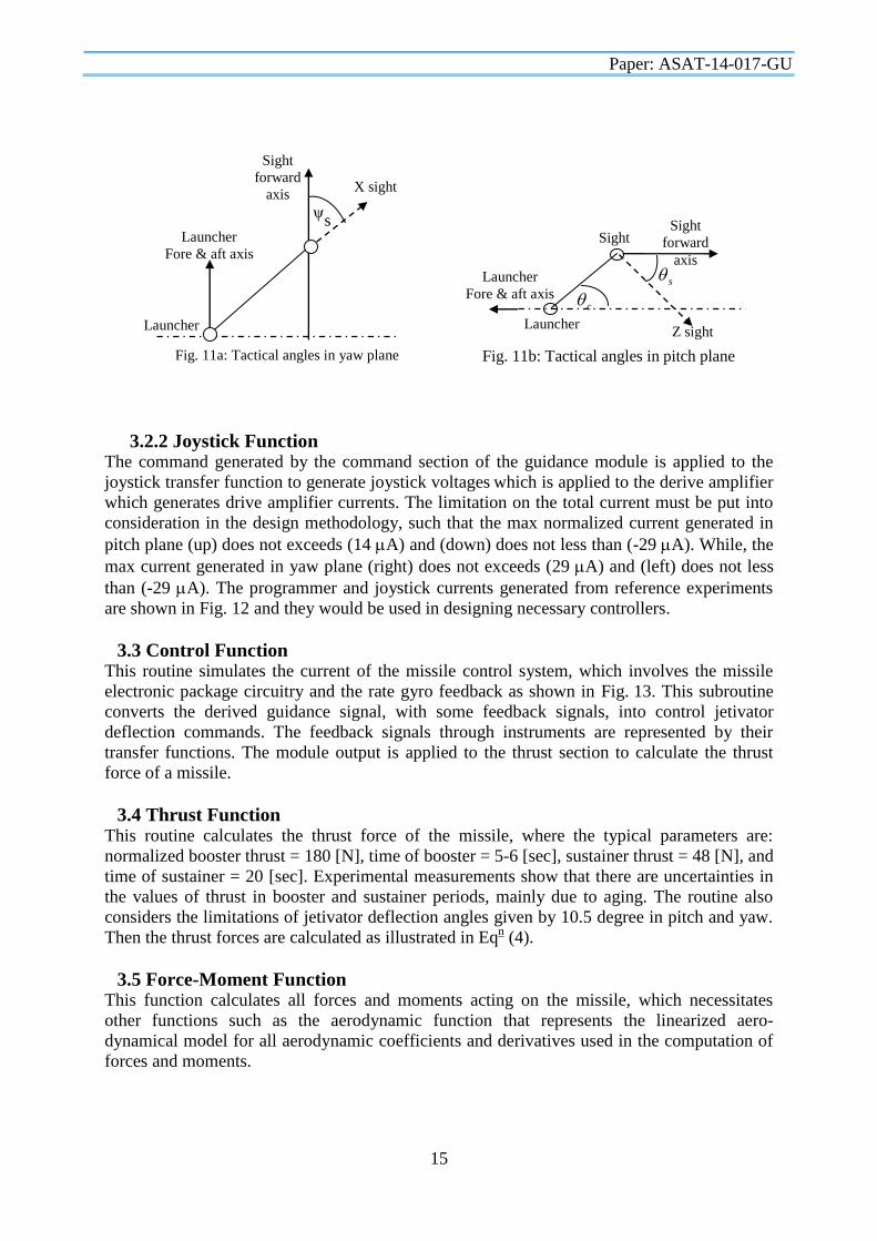
where K1= 0.3 if time of flight < Ty and zero if time of flight > Ty, Ty is the end of gathering
to sight line phase of engagement, and s is the angle between sight forward axis and LOS in
yaw plane as shown in Fig. 11a. Similarly, the elevation programmer equations are:
ssB
sA
/t
BAp
KE
)66.3(35
)e(
(26)
where =2.5 sec, Ks=0.15, Eo is the temperature compensation term (13.7 normally), θc is
the crest angle, and θs is the angle between sight forward axis and LOS in pitch plane as
shown in Fig. 11b.
Start
sequence
Sequence
Unit
Controller
Sightin
g Unit Missile
Programmer
Electronic
Control
(PEC)
Error
command Initial
Conditions
Setting LOS
data
Guidance
Commands
Fig. 10: Programmer function in guidance and control
Programmer
Ψs
Θs
Joystick
Joystick
current
yaw
current
Fig. 9: Guidance section
Drive amplifier Pitch Yaw
Commands
Total current pitch
current
Paper: ASAT-14-017-GU
15
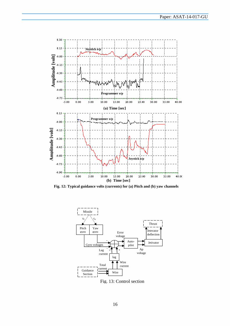
3.2.2 Joystick Function The command generated by the command section of the guidance module is applied to the
joystick transfer function to generate joystick voltages which is applied to the derive amplifier
which generates drive amplifier currents. The limitation on the total current must be put into
consideration in the design methodology, such that the max normalized current generated in
pitch plane (up) does not exceeds (14 A) and (down) does not less than (-29 A). While, the
max current generated in yaw plane (right) does not exceeds (29 A) and (left) does not less
than (-29 A). The programmer and joystick currents generated from reference experiments
are shown in Fig. 12 and they would be used in designing necessary controllers.
3.3 Control Function This routine simulates the current of the missile control system, which involves the missile
electronic package circuitry and the rate gyro feedback as shown in Fig. 13. This subroutine
converts the derived guidance signal, with some feedback signals, into control jetivator
deflection commands. The feedback signals through instruments are represented by their
transfer functions. The module output is applied to the thrust section to calculate the thrust
force of a missile.
3.4 Thrust Function This routine calculates the thrust force of the missile, where the typical parameters are:
normalized booster thrust = 180 [N], time of booster = 5-6 [sec], sustainer thrust = 48 [N], and
time of sustainer = 20 [sec]. Experimental measurements show that there are uncertainties in
the values of thrust in booster and sustainer periods, mainly due to aging. The routine also
considers the limitations of jetivator deflection angles given by 10.5 degree in pitch and yaw.
Then the thrust forces are calculated as illustrated in Eqn (4).
3.5 Force-Moment Function This function calculates all forces and moments acting on the missile, which necessitates
other functions such as the aerodynamic function that represents the linearized aero-
dynamical model for all aerodynamic coefficients and derivatives used in the computation of
forces and moments.
Launcher
Fore & aft axis
Launcher
Sight
forward
axis X sight
Fig. 11a: Tactical angles in yaw plane
sψ
Sight
forward
axis
Sight
Fig. 11b: Tactical angles in pitch plane
s Launcher
Fore & aft axis
Z sight Launcher
c
Paper: ASAT-14-017-GU
16
Fig. 12: Typical guidance volts (currents) for (a) Pitch and (b) yaw channels
Joystick o/p
Am
pli
tud
e [v
olt
]
Programmer o/p
(a) Time [sec]
Joystick o/p
(b) Time [sec]
Am
pli
tud
e [v
olt
]
Programmer o/p
-
-
Pitch gyro
Yaw gyro
Missile
Wire
lag
Guidance
Section
Auto-
pilot Jetivator
Thrust
Jetevator
deflection
Ap
voltage
Error
voltage
Wire
current
Lag
current
Gyro voltages
Total
current
+ +
Fig. 13: Control section
r r
Paper: ASAT-14-017-GU
17
3.6 Aerodynamic Function
This routine calculates the resultant missile speed mV which is given by:
222 wvuvM (27)
where U, V, and W are the velocity components along board coordinate axes. Also the
aerodynamic force and moment coefficients are usually defined as functions of angle of attack
(), sideslip angle (), and other flight parameters. In reference to Fig. 3, the relationships
between the velocity components and the firing angles are:
)/(tan
)/(tan
1
1
uv
uw
(28)
Note that the missile function solves Euler’s equations via calling other necessary functions
including transformation, gravity, and forces and moments.
3.7 Auxiliary Modules There are some auxiliary functions including Initialize module that is devoted to initialize all
the missile and target initial states (position, velocity, and acceleration) with different gains
for the guidance and control loops; the Integration module which uses a fourth order runge-
kutta method to perform the numerical integration for all the states of differential equations
describing the model; the Output module where output parameters describing the behavior of
the system are stored and used for the system performance analysis; the Rotate module that is
used to calculate the transformation matrix from board to reference coordinate system or its
transpose; and the Miss-distance module which is devoted to calculate the miss-distance (the
closest distance between the target and the missile).
4. Flight Simulation Analysis This section is devoted for evaluating pre-calculated parameters (aerodynamic and dynamic
parameters) to get a fair match between the simulated and real flight trajectories. It yields the
appropriate and more accurate model that can be used for the guidance and control design,
discussed later in the next two paper-parts.
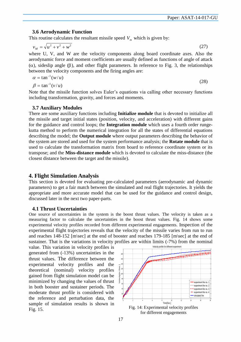
4.1 Thrust Uncertainties One source of uncertainties in the system is the boost thrust values. The velocity is taken as a
measuring factor to calculate the uncertainties in the boost thrust values. Fig. 14 shows some
experimental velocity profiles recorded from different experimental engagements. Inspection of the
experimental flight trajectories reveals that the velocity of the missile varies from run to run
and reaches 148-152 [m\sec] at the end of booster and reaches 179-185 [m\sec] at the end of
sustainer. That is the variations in velocity profiles are within limits (-7%) from the nominal
value. This variation in velocity profiles is
generated from (-13%) uncertainties in the
thrust values. The difference between the
experimental velocity profiles and the
theoretical (nominal) velocity profiles
gained from flight simulation model can be
minimized by changing the values of thrust
in both booster and sustainer periods. The
moderate thrust profile is considered with
the reference and perturbation data, the
sample of simulation results is shown in
Fig. 15. Fig. 14: Experimental velocity profiles
for different engagements
0 2 4 6 8 10 12 14 16 180
20
40
60
80
100
120
140
160
180
Time[Sec.]
Ve
locity[m
.\S
ec.]
Velocity profile for different experiment
experiment fire no. 1
experiment fire no. 2
experiment fire no. 3
experiment fire no. 4
simulated fire
Paper: ASAT-14-017-GU
18
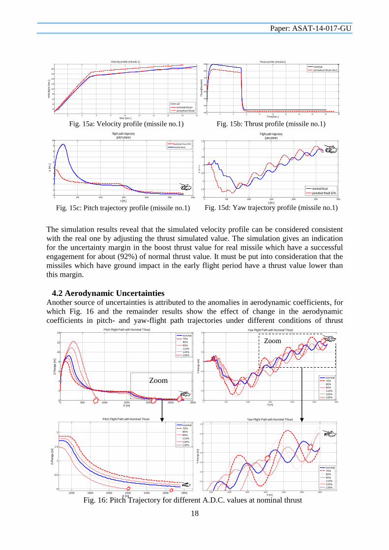
The simulation results reveal that the simulated velocity profile can be considered consistent
with the real one by adjusting the thrust simulated value. The simulation gives an indication
for the uncertainty margin in the boost thrust value for real missile which have a successful
engagement for about (92%) of normal thrust value. It must be put into consideration that the
missiles which have ground impact in the early flight period have a thrust value lower than
this margin.
4.2 Aerodynamic Uncertainties Another source of uncertainties is attributed to the anomalies in aerodynamic coefficients, for
which Fig. 16 and the remainder results show the effect of change in the aerodynamic
coefficients in pitch- and yaw-flight path trajectories under different conditions of thrust
1600 1800 2000 2200 2400 2600 2800
0.2
0.4
0.6
0.8
1
1.2
1.4
X [m]
Y-R
an
ge
[m
]
Yaw Flight Path with Nominal Thrust
nominal
70%
80%
90%
110%
120%
130%
0 500 1000 1500 2000 2500 30000
2
4
6
8
10
12
14 Pitch Flight Path with Nominal Thrust
X [m]
Z-R
ange [m
]
nominal
70%
80%
90%
110%
120%
130%
1600 1800 2000 2200 2400 2600 2800
0
0.5
1
1.5
2
Pitch Flight Path with Nominal Thrust
X [m]
Z-R
ange [m
]
nominal
70%
80%
90%
110%
120%
130%
Fig. 16: Pitch Trajectory for different A.D.C. values at nominal thrust
Zoom
0 500 1000 1500 2000 2500 3000-2
-1.5
-1
-0.5
0
0.5
1
1.5
X [m]
Y-R
an
ge
[m
]
Yaw Flight Path with Nominal Thrust
nominal
70%
80%
90%
110%
120%
130%
Zoom
Fig. 15a: Velocity profile (missile no.1)
2 4 6 8 10 12 14 16 18 20
20
40
60
80
100
120
140
160
180
time [sec.]
ve
locity[m
.\se
c.]
Velocity profile (missile 1)
ref
nominal thrust
perturbed thrust
Fig. 15b: Thrust profile (missile no.1)
0 2 4 6 8 10 12 14 16 18 20200
300
400
500
600
700
800
900
Time[Sec.]
Th
rust[N
ew
ton
]
Thrust profile (missile1)
nominal
perturbed thrust mis1
0 500 1000 1500 2000 2500 3000-2
-1.5
-1
-0.5
0
0.5
1
1.5
x [m.]
y [m
.]
Flight path trajectory(yaw plane)
nominal thrust
perturbed thrudt 92%
Fig. 15d: Yaw trajectory profile (missile no.1)
Fig. 15c: Pitch trajectory profile (missile no.1)
0 500 1000 1500 2000 2500 30000
1
2
3
4
5
6
7
8
9
10
x [m.]
-z [m
.]
filght path trajectory(pitch plane)
perturbed thrust 92%
nominal thrust

Paper: ASAT-14-017-GU
19
value. It can be noticed that the difference in miss distance obtained from different cases and
the cases where the ground impact occurred. For nominal thrust value the ground impact
occurred at +10% of aerodynamics coefficient in 2670 meter and at +20% in 2190 meter and
at +30% in 852 meter and for -14% thrust value the ground impact occurred at +10% of
aerodynamics coefficient in 575 meter and at +20% in 542 meter and at +30% in 2330 meter.
In other words the figure reveals that the change in aerodynamic coefficients can be
considered as one source of uncertainties in the desired system.
4.3 Wind Velocity The third source of uncertainties is attributed to the effect of wind velocity. Thus, Figs
(17,18,19) show the effect of wind velocity on the missile flight path trajectories i.e. wind
velocities in x, y, and z directions can be considered as a source of uncertainties in this work.
Wind velocity in X-direction
Wind velocity in Y-direction
Wind velocity in Z direction
0 500 1000 1500 2000 2500 3000-10
-8
-6
-4
-2
0
2
X [m]
Y [m
]
Yaw Flight Path with 90% Thrust
0 (m/sec)
20 (m/sec)
40 (m/sec)
60 (m/sec)
-10 (m/sec)
-20 (m/sec)
-30 (m/sec)
0 500 1000 1500 2000 2500 3000-1
0
1
2
3
4
5
6
7
8
X [m]
-Z [m
]
Pitch Flight Path with 90% Thrust
0 (m/sec)
20 (m/sec)
40 (m/sec)
60 (m/sec)
-10 (m/sec)
-20 (m/sec)
-30 (m/sec)
Fig. 17: Pitch and Yaw Trajectories at 90% thrust for different Vwx
0 500 1000 1500 2000 2500 3000-1.5
-1
-0.5
0
0.5
1
1.5
X [m]
Y [m
]
Yaw Flight Path with Nominal Thrust
0 (m/sec)
+-20 (m/sec)
+-40 (m/sec)
+-60 (m/sec)
0 500 1000 1500 2000 2500 3000-2
0
2
4
6
8
10
12
14
16
X [m]
-Z [m
]
Pitch Flight Path with Nominal Thrust
0 (m/sec)
+-20 (m/sec)
+-40 (m/sec)
+-60 (m/sec)
Fig. 18: Pitch and Yaw Trajectories at nominal thrust for different Vwy
0 500 1000 1500 2000 2500 3000-2
0
2
4
6
8
10
12
14
16
X [m]
-Z [m
]
Pitch Flight Path with Nominal Thrust
0 (m/sec)
20 (m/sec)
40 (m/sec)
60 (m/sec)
-20 (m/sec)
-40 (m/sec)
-60 (m/sec)
0 500 1000 1500 2000 2500 3000-1.5
-1
-0.5
0
0.5
1
1.5
X [m]
Y [m
]
Yaw Flight Path with Nominal Thrust
0 (m/sec)
20 (m/sec)
40 (m/sec)
60 (m/sec)
-20 (m/sec)
-40 (m/sec)
-60 (m/sec)
Fig. 19: Pitch and Yaw Trajectories at nominal thrust for different Vwz

Paper: ASAT-14-017-GU
20
4.5 Evaluation of the Flight Simulation Model Let us now evaluate the established flight
simulation model by comparing its output
flight path trajectory with reference
trajectories. The simulation is conducted
with nominal and perturbed values and
depicted with the reference as shown in
Fig. 20. This Figure reveals that the
established flight simulation which had
programmed within both C++ and
MATLAB environments yield trajectories
that are nearly consistent with reference
trajectories.
5. Conclusion The paper presented the modeling of the
intended system concerning the reference
frames, coordinates’ transformations and
equations of motion. This model is built in
the form of modules assigned to each
process within the guided missile system.
Then, it is programmed within the C++
and MATLAB environments. The
simulation is conducted with different
engagement scenarios and different
sources of uncertainties including thrust
variation, errors in aerodynamic
coefficients and wind velocity effects. The
simulation results are validated against
reference data with different levels of
uncertainty which clarify appropriateness
of built 6DOF model for autopilot and
guidance laws design with the hardware-
in-the-loop (HIL); the objective of next
papers.
6. References [1] Abd-Altief, M.A., G.A. El-Sheikh and M.Y. Dogheish, Anti-Tank Guided Missile
Performance Enhancement; Part-1: Hardware in the Loop Simulation, 5th ICEENG
Conference, GC-9, MTC, Cairo, Egypt, May 16-18, 2006.
[2] Abd El-Latif, M.A., Robust Guidance and Control Algorithms in Presence of
Uncertainties, MSc Thesis, Guidance Department, M.T.C., Cairo, Egypt, 2006.
[3] Aly, M.S., Dynamical Analysis of Anti-Tank Missile Systems, Proceedings of the 9th
int. AMME conference, 16-18 May, 2000.
[4] Aly, M.S., Linear Model Evaluation of Command Guidance Systems, Proceedings of
the 8th Int. conference on aerospace science and aviation technology, pp 1001-1003, 4-6
May, 1999.
0 500 1000 1500 2000 2500 3000-1.5
-1
-0.5
0
0.5
1
1.5
X [m]
Y [m
]
Yaw Flight Path
Matatlab simulation
C++ simulation
0 500 1000 1500 2000 2500 30000
1
2
3
4
5
6
7
8
9
10
X [m]
-Z [m
]
Pitch Flight Path
Matlab simulation
C++ simulation
0 500 1000 1500 2000 2500 3000-4
-2
0
2
4
6
8
X [m]
Y [m
]
Yaw Flight Path
Ref1
Ref2
Ref3
Ref4
sim nominal thrust
sim perturbed thrust 95%
0 500 1000 1500 2000 2500 30000
2
4
6
8
10
12
X [m]
-Z [m
]
Pitch Flight Path
Ref1
Ref2
Ref3
Ref4
sim perturbed thrust 95%
sim nominal thrust
(a)
(b)
(c)
(d) Fig. 20: Flight simulation and reference trajectories
(a) Pitch Ref. & MATLAB (b) Yaw Ref. & MATLAB
(c ) Pitch C++ & MATLAB (d) Yaw C++ & MATLAB
Paper: ASAT-14-017-GU
21
[5] El-Halwagy, Y.Z., M.S. Aly, and M.S. Ghoniemy, Command Guidance System
Simulation Airframe Analysis, Proceedings of the 7th Int. conference on aerospace
science and aviation technology, 13-15 May, 1997.
[6] El-Sheikh, G.A., Theory of Guidance and Systems, MTC, 2004, 2010.
[7] El-Sheikh, G.A., M.A. Abd-Altief and M.Y. Dogheish, Anti-Tank Guided Missile
Performance Enhancement; Part-2: Robust Controller Design, 5th ICEENG Conference,
GC-10, MTC, Cairo, Egypt, May 16-18, 2006.
[8] El-Sheikh, G.A., R.A. Elbardeny and N. Maher, Robust Guidance for CLOS System,
12th International Conference on Aerospace Sciences and Aviation Technology
(ICASAT12), M.T.C., Cairo, Egypt, May 28-30, 2007 (GUD08-229).
[9] Emil J.E., Test and Evaluation of Tactical Missiles, John Willey & Sons, (1995).
[10] Etkin B., Dynamics of Flight, Jhon Willey and Sons Inc., 1972.
[11] Garnell P. and East D. J., Guided Weapon Control Systems, 2nd edition, Pergamon
press, New York, 1980.
[12] Hertfordshire, S., Guided Weapons, British aircraft corporation, England, May, 1975.
[13] Locke S. and East D.J., Principles Of Guided Missile Design, Van Nostrand Reinhold
company Inc., 1955.
[14] Michael selig, Brian fucsz, Flight Simulation, May, 2003.
[15] Oda, A.N., Fuzzy Logic Control and its Application in Guidance Systems, MSc Thesis,
Guidance Department, M.T.C., Cairo, Egypt, September, 2005.
[16] Ramadan, N.M., Performance Enhancement of an Anti-Tank Guided Missile Via
Advanced Techniques, MSc Thesis, Guidance Department, M.T.C., Cairo, Egypt,
September, 2007.


