
Pricing Over the Product Life Cycle: An Empirical Analysis
*The authors gratefully acknowledge the Bureau of Economic Analysis (BEA) and NPD Techworld, as well as the James M. Kilts Center, Graduate School of Business, University of Chicago who made data available for this project. Any opinions expressed in the paper are those of the authors.
Daniel Melser*Department of Economics
Monash UniversityCaulfield, VIC 3145
Australia
Iqbal SyedSchool of Economics
University of New South WalesSydney, NSW 2052
Australia

1. The Aims of the Paper Empirically estimate the ‘age effect’ on a
product’s price
Undertake some simulations of the effect of new and disappearing goods on price indexes

1.1. Intertemporal Price Discrimination (IPD) & Reasons for Life Cycle Pricing
Profitable for a firm if there exists heterogeneity in consumer demand
Institutional factors, market structure can lead to IPD Koh (2006), Varian (1989), Stokey (1979)
Other factors: marketing strategy cost reduction product customization degree of competition Firms may charge a lower price relative to substitutes to
overcome consumer inertia
The "age effect" combines all the above factors

1.2. Price Indexes and the Product Life Cycle Why does it matter?
Sampling Representativeness Quality Adjustment
Price
Age
Life Cycle Price Effect
Price
Time

1.2. Price Indexes and the Product Life Cycle (cont’d) Age effect has important implications:
Boskin Commission (Gordon and Griliches, 1997) The Schultze Report (Schultze and Mackie, 2002) ILO-CPI Manual (2004)
Examples: Armkneckt (1997) provides an example of video recorders
included in the US CPI in 1987 ($500) but available from 1978 ($1200)
Cell phones (Hausman, 1999) Microwaves and air conditioners (Gordon and Griliches,
1997)
Bias can be large as all goods age and turnover rates can be high and applicable to both fixed basket and cost-of-living indexes

2. Modeling Life Cycle Pricing The general model:
What functional form for the life cycle effects?
ititditait
T
iti
I
it edfafhbp
)()()ln(21
""for dummy time
""for dummy product
price
it
it
it
h
b
p
death toage
appearance from age
it
it
d
a

2.1. Which Functional Form? A polynomial function:
A non-parametric dummy variable function:
We decided on Splines!
...)( 33
221 itititita aaaaf
,)(1
aitjaj
J
jita uaf
1aitju itaj if

2.2. Splines Functions and can take any form but
they should be (in some sense) smooth
We solve the optimization problem:
)( ita af )( itd df
2
11obs. all
)()()ln(.min
itditait
T
it
I
it dfafhbp
dxxfdxxf da2"
22"
1 )]([)]([

2.3. Why Splines? Unique solutions exist (Wahba, 1990; Green and
Silverman, 2000)
Extremely flexible functional form
Relationship with dummy variable and polynomial regression:
itita
aitjaj
J
jita
aaf
uaf
11
11
)( ,
)( ,0

2.4. The Smoothing Parameters Choice of and influence the smoothness of
the estimated functions Cross Validation (CV):
Generalized Cross Validation (GCV):
1 2
,1
),(ˆ
,)],(ˆ[),(
2
21
1
221
121
nn
nnN
n
nn
N
n
yy
yyCV
A
yy Aˆ
2
121
121 )(tr1
),(ˆ),(
AN
yyGCV nn
N
n
)ln( nn py
3. An Empirical Investigation Estimate the spline-smoothing model
Undertake some simulations to estimate the effect on price indexes of life cycle price trends

3.1. The Data Two data sources:
Bureau of Economic Analysis (BEA) and NPD Techworld scanner data for high-tech goods:
Desktop computers Laptop computers Personal digital assistants (PDAs)
Dominick’s Fine Foods scanner data. Large US supermarket based in Chicago
Beer Canned soup Cereal

3.1. The Data (cont’d) An Example of the data:
Time
Product 1 2 3 4 5 6 7
A X X X X X
B X X X X X X
C X X X X X
D X X X X X X X
…

3.1. The Data (cont’d) An Example of the data:
Time
Product 1 2 3 4 5 6 7
A X(a=0, d=5)
X (a=0, d=4)
X (a=0, d=3)
X (a=0, d=2)
X(a=0, d=1)
B X(a=1, d=0)
X(a=2, d=0)
X(a=3, d=0)
X(a=4, d=0)
X(a=5, d=0)
X(a=6, d=0)
C X(a=0, d=0)
X(a=0, d=0)
X(a=0, d=0)
X(a=0, d=0)
X(a=0, d=0)
D X(a=0, d=0)
X(a=0, d=0)
X(a=0, d=0)
X(a=0, d=0)
X(a=0, d=0)
X(a=0, d=0)
X(a=0, d=0)
…

3.2. Summary StatisticsProduct Probability that a model Disappears
from the market in: Number of Products Average
Length of Product Life # (months)
1 month 6 months 12 months Total Appeared Disappeared
Desktops 28.13% 50.94% 67.33% 2427 711 (31.80%)
426 (17.6%)
7.04
Laptops 26.34% 50.24% 66.15% 2451 813 (33.2%)
489(20.0%)
6.24
PDAs 9.68% 17.70% 28.23% 234 87 (37.2%)
22 (9.4%)
3.88
Beer 5.17% 14.98% 25.38% 752 142 (18.9%)
289 (38.4%)
17.84
Canned Soup
2.16% 8.42% 15.56% 442 115 (26.0%)
214 (48.4%)
25.97
Cereal 2.79% 9.86% 15.56% 480 76 (15.8%)
122 (25.4%)
19.91
goods.tech -high for the months 3 and productst supermarke for the
months 6n longer tha wascycle life thefor which and cycle life theof end andstart both the observed wefor which products allFor #
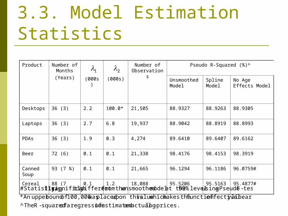
3.3. Model Estimation Statistics
Product Number of Months(Years) (000s) (000s)
Number of Observations
Pseudo R-Squared (%)^
Unsmoothed Model
Spline Model
No Age Effects Model
Desktops 36 (3) 2.2 100.0* 21,505 88.9327 88.9263 88.9305
Laptops 36 (3) 2.7 6.8 19,937 88.9042 88.8919 88.8993
PDAs 36 (3) 1.9 0.3 4,274 89.6410 89.6407 89.6162
Beer 72 (6) 0.1 0.1 21,338 98.4176 98.4153 98.3919
Canned Soup
93 (7 ¾) 0.1 0.1 21,665 96.1294 96.1186 96.0759#
Cereal 88 (7 1/3) 0.1 1.2 18,088 95.5206 95.5163 95.4877#
1 2
prices.-log actualon estimated of regression a of squared-R The ^
linear.y effectivelfunction themakes which valueupon this placed was100,000 of boundupper An *
test.-F Pseudo a using level 99% at the model unsmoothed thefromdifferent tly significanlly Statistica #

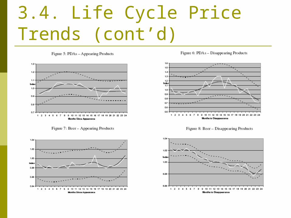
3.4. Life Cycle Price Trends Effect of life cycle price trends are quite
large though results are often not statistically significant, confidence intervals are wide
Pricing lip for the high tech goods
The beginning and end of the product life cycle do tend to exhibit pricing extremes

3.4. Life Cycle Price Trends (cont’d)
3.4. Life Cycle Price Trends (cont’d)

3.4. Life Cycle Price Trends (cont’d)
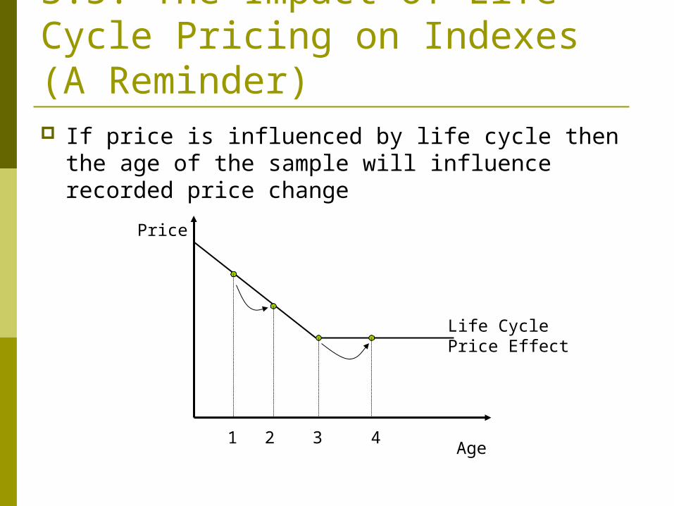
3.5. The Impact of Life Cycle Pricing on Indexes (A Reminder) If price is influenced by life cycle then the age of
the sample will influence recorded price change
Price
Age
Life Cycle Price Effect
1 2 3 4

3.6. Implications for Price Indexes What does the price index look like? Under a
matched sample:
dmk
M
mdkamk
M
mak
djdjdj
J
jajajaj
J
j
M
mmmm
mmmmM
m
uM
uuM
u
uuuu
dahbp
dahbpP
11
11
11
01
1
0
1
101
1 ,
1 where
)(ˆexp)(ˆexp)ˆˆexp(
),,,(ˆ)1,1,,(ˆˆ

3.7. Simulations of the Effects on Price Indexes
(A) The empirical distribution of products for which we observed the entire life cycle.
(B) A uniform distribution of products is sampled for a 12-month period over the ages, 1 month to 12 months for new goods. We further supposed that these products were uniformly distributed as being between 12 to 23 months (inclusive) to disappearing from the market.
(C) A uniform distribution of products is sampled over a 6 month period from the ages 7 to 12 months for new goods and we supposed that these products had between 18 to 23 months (inclusive) to go in their life until they disappeared.

3.8. The Effects on Recorded Price Change
Product (A) (B) (C)
New Goods
Dis. Goods
Total New Goods
Dis. Goods
Total New Goods
Dis. Goods
Total
Desktops -6.57 -2.12 -33.98 -8.00 -5.39 -37.16 -8.83 -5.39 -37.73
Laptops -11.38 0.75 -46.17 -11.70 0.41 -46.54 -10.72 -4.31 -48.49
PDAs -1.80 -10.44 -30.46 -3.04 -4.02 -26.42 -8.10 12.45 -18.30
Beer 0.86 -0.60 2.05 0.42 2.13 4.4 0.16 1.94 3.93
CannedSoup
-3.52 1.90 4.04 -3.40 -0.55 1.66 -3.33 0.66 2.97
Cereal -1.75 2.43 3.04 -1.92 0.66 1.08 -0.55 1.00 2.84

4. Summary and Conclusions The effects of life cycle on price are large
though in some cases statistically insignificant
The sample of products in a price index, i.e. how many ‘young’ and ‘old’ items, influences recorded price change
Effort needs to go into ensuring that the sample of product's ages accurately reflects that in the population


