
Political Uncertainty, Public Expenditure and Growth
Julia Darby
Chol-Won Li
and
V. Anton Muscatelli
University of Glasgow
Correspondence to:Julia Darby,Dept. of Economics,Adam Smith Building,University of Glasgow,Glasgow G12 8RT,United Kingdom.Tel: +44 141 330 4692Fax: +44 141 330 4940Email: J. [email protected]
1
1. Introduction
There are a number of channels through which political instability can affect
economic growth. One obvious channel is the impact which greater social unrest and
political upheaval and revolution can have on the incentives to invest. It is quite
apparent that the lack of protection for property rights may harm the prospects for
private investment1, and may reduce foreign direct investment in a country2. Similarly,
in countries where rulers are weak and run the danger of being overthrown, they might
have an incentive to allow key groups to engage in rent-seeking activities, which may
again harm economic growth3. There seems to be considerable empirical evidence that
major political upheaval (as opposed to routine changes of governments following
elections) and coups d’etat can adversely affect economic growth (see Alesina et al.,
1996, Barro, 1996, and Easterly and Rebelo, 1993).
In modern democracies, where government changes are generally peaceful and
follow constitutional norms, political instability may still have an impact on economic
growth. The main mechanism at work in these models is through the impact of political
instability on government myopia: forward-looking governments which have uncertain
prospects of re-election may not be interested in carrying out long-term economic
policies4. For instance, Svensson (1993) emphasises how governments may be less
inclined to make improvements to the legal system. Calvo and Drazen (1997) show
how policy uncertainty can distort the future path of investment decisions. In Devereux
and Wen (1996) political instability encourages governments to run down the
1 For theoretical models in which the lack of enforcement of property rights affects growth, see Tornelland Velasco (1992) and Benhabib and Rustichini (1996). For a survey, see Persson and Tabellini(1998).2 See Rodrik (1991).3 See Murphy et al. (1991).

2
economy’s asset base, thus encouraging future governments to increase capital taxation
with the result that private investment, expecting higher future taxation, is reduced.
Persson and Tabellini (1998) build a 2-period model in which capital taxation is used to
finance public investment, which drives economic growth and enhances the future tax
base. The problem is that public investment is less valuable for an incumbent
government if re-election is uncertain, because less of the economy’s future tax
revenues will be spent on the incumbent’s preferred public goods. Hence political
instability (a greater uncertainty of re-election for the incumbent) reduces public
investment because it increases policy myopia.
Empirically, there seems to be evidence in favour of a negative link between
minor political instability (the frequency of changes in a government’s political
complexion) and economic growth (see Alesina et al., 1996, Perotti, 1996).
In this paper, we focus on the link between the political instability (due to
uncertainty in electoral outcomes) and economic growth through the impact on a
government’s decisions on how to allocate government expenditure between public
consumption and public investment. The value added of our contribution is the
following. First, unlike some existing two-period models of the impact of political
uncertainty on growth (see Persson and Tabellini, 1998) we propose an infinite horizon
model where a particular equilibrium is generated by the dynamic interaction of an
endogenous growth model with political dynamics. In two-period models government
myopia generally arises because incumbent governments face a probability of not having
access to the future benefits from current taxation and spending decisions for their
political constituency. In our model, government myopia arises because of office
4 The notion of policy myopia is quite common in political economy models. For alternative models offiscal policy in which the incumbent has an incentive not to act in the social interest see Alesina andTabellini (1990) and Milesi-Ferretti and Spolaore (1994).
3
motivation, so that an incumbent government will perceive a more limited political
benefit from decisions taken now which only impact with a lag on consumer utility.
Thus political uncertainty leads to a shift of government budgets from capital spending
to government consumption.
Second, unlike other attempts to model political uncertainty, we provide a full
account of the preferences of consumers and how these affect the political equilibrium.
The advantage of this is that we are able to compare the stochastic steady-state growth
equilibrium under political uncertainty with that which would prevail in the presence of
an optimal social planner. This allows us to consider the welfare implications of political
uncertainty for the median voter.
Third, our focus is not only on the impact of the political environment for
taxation decisions, but also on the allocation of government spending between
government investment and consumption. Thus, our focus is rather different from that
in other contributions to this area which tend to concentrate on inequality5, the
enforcement of property rights, and public expenditures on different types of public
goods. As explained below, we believe that the focus on the relationship between public
investment and consumption is an important one, especially in the OECD economies.
The rest of this paper is structured as follows. In Section 2 we motivate our
focus on the relationship between public investment and consumption. In Section 3 we
outline our theoretical model and the main results. Section 4 concludes.
5 See for example Saint Paul and Verdier (1993), Perotti (1993).

4
2. The Relationship Between Government Investment and Growth
There is strong empirical evidence that government spending can have a
significant impact on productivity growth both from production function estimates (see
inter alia Aschauer, 1989, Munnell, 1990, Morrison and Schwartz, 1992)6. Work on
cross-country panel studies show some evidence in favour of the hypothesis that
spending on public infrastructure such as transport and communications enhances
growth prospects (see Easterly and Rebelo, 1993), whilst the evidence on public
educational spending tends to be more mixed (see Barro, 1996). In contrast, most
studies tend to find a negative impact of government consumption on economic growth
(see Barro, 1996)7.
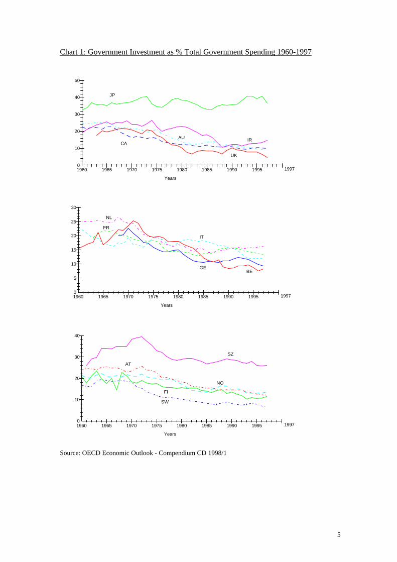
One striking piece of casual empirical evidence from the post World War II
war era is the rise in the proportion of current expenditures in total government
spending in many of the OECD economies. Chart 1 shows how the proportion of
government investment in total government spending has evolved in a number of OECD
countries since 19608. In particular the increase in government consumption and
transfers has been widespread amongst OECD economies since the mid-1960s (see
Alesina and Perotti, 1996). The other notable feature of government budgets in the
OECD economies is that many of the attempts to stabilise increasing debt burdens in the
late 1980s and 1990s have resulted in increases in taxation and in cuts in capital outlays.
There are of course exceptions to this (especially the fiscal adjustment in Ireland in
6 Although the size of the total impact of public capital spending on productivity growth is a matter ofsome debate (see Holtz-Eakin and Schwartz, 1994) and obviously varies between countries and sectors.7 For some contrary evidence from developing countries where sometimes capital spending ismisallocated, see Devarajan et al. (1996).8 The countries considered are Australia (AU), Austria (AT), Belgium (BE), Canada (CA), Finland(FI), France (FR), Germany (GE), Ireland (IR), Italy (IT), Japan (JP), Netherlands (NL), Norway (NO),Sweden (SW), Switzerland (SZ) and the United Kingdom (UK). We have excluded small countries likeLuxembourg, Israel and Iceland from our analysis.
5
Chart 1: Government Investment as % Total Government Spending 1960-1997
CA
JP
AU
UK
IR
Years
0
10
20
30
40
50
1960 1965 1970 1975 1980 1985 1990 1995 1997
GE
FR
IT
BE
NL
Years
0
5
10
15
20
25
30
1960 1965 1970 1975 1980 1985 1990 1995 1997
SW
FI
NO
AT
SZ
Years
0
10
20
30
40
1960 1965 1970 1975 1980 1985 1990 1995 1997
Source: OECD Economic Outlook - Compendium CD 1998/1

6
1987-89), and it has been pointed out by Alesina and Perotti (1996, 1997) that most
successful (i.e. long-lasting) fiscal adjustments tend to concentrate on cutting
government transfers and consumption whilst most unsuccessful fiscal adjustments tend
to result from cuts in capital expenditures. They also report that, following successful
adjustments, there is a tendency for private investments to boom9.
This rise in the share of government consumption in GDP (and the consequent
fall in government investment) has coincided with a slow-down in productivity growth.
Table 1 shows how labour productivity and total factor productivity growth has evolved
for a number of OECD countries since the 1960s.
Table 1: Productivity in the Business Sector
Total Factor Productivity Labour Productivity1960-19731 1973-1979 1979-19962 1960-1973 1973-1979 1979-1996
CA 1.1 -0.1 -0.6 2.5 1.1 0.9JP 5.6 1.1 1.2 8.4 2.8 2.3AU 2.2 1.2 0.9 3.1 2.5 1.3GE4 2.6 1.8 0.6 4.5 3.1 1.2FR 3.7 1.6 1.3 5.3 2.9 2.2IT 4.4 2.0 1.2 6.4 2.8 2.1UK 2.8 0.7 1.2 4.2 1.6 1.7IR 4.6 3.9 3.6 4.8 4.3 4.1BE 3.8 1.3 1.0 5.2 2.7 1.9NL 3.5 1.7 1.0 4.8 2.6 1.5NO3 2.2 1.3 0.6 3.8 2.7 1.8SW 1.9 0.0 1.2 3.7 1.4 2.0FI 4.0 1.9 2.6 5.0 3.2 3.6SZ 1.5 -0.7 -0.1 3.3 0.8 0.4AT 3.2 1.1 1.0 5.7 3.1 2.3
Notes:1 1960 or earliest year available: IR 1961; JP UK 1962; FR SW 1965; CA AU NO 1966; NL 1969;
BE 1970.2 1996 or latest year available: AT NO 1994; IT AU FI IR SZ 1995.3 Norway: mainland business sector - excludes shipping and crude petroleum and gas extraction.4 Germany: Pre-1979 is W.Germany, 1979-96 is calculated as the average of W.German productivity
growth between 1979 and 1991 and total German productivity growth between 1991 and the mostrecent year available.
5 Labour Productivity is output per employed person. TFP growth is a weighted average of growth inlabour and capital productivity. Sample-period averages for capital and labour shares are used as
weights.
Source: OECD Economic Outlook June 1998 (Annex Table 59).
9 For an outline and evidence of possible non-Keynesian effects of fiscal expansions and contractions(particularly involving government consumption), see Giavazzi and Pagano (1990, 1995).
7
Obviously one has to be careful in interpreting any causal links, but in a number
of countries there has been a renewed emphasis on changing fiscal policies to ‘take a
longer term view’, and this generally involves a reallocation towards capital
expenditures. In the UK, the first Budget of the new Labour government brought with it
a commitment towards a ‘golden rule’ of public spending, whereby deficit spending
would only be allowed (over the cycle) on public investment. It remains to be seen how
effective such measures are, as ‘golden rules’ for fiscal policy have been circumvented
in the past (cf. the case of Germany), but the conventional wisdom is that long-term
economic success requires a reallocation of government spending towards public
investment.
There is one missing empirical link in this account: that which runs from political
instability to government spending decisions. Here one has to rely on more qualitative
evidence. Most of the empirical evidence on the links between political complexion of
governments tends to focus on the impact of political uncertainty on fiscal deficits or
total government spending (see Roubini and Sachs, 1989a,b, Grilli et al., 1991, and
Alesina and Perotti, 1996). The general findings are that coalition governments tend,
with some exceptions, to be less fiscally responsible10.
Data is of course available on the frequency of government changes and the
complexion of the incumbent government in OECD countries which are non-
presidential democracies (see Woldendorp et al., 1993). However, one difficulty in
measuring the degree of political uncertainty from the frequency of ‘government
changes’ which have occurred ex post is that this does not provide a measure of the ex
ante degree of political uncertainty and external competition experienced by the
incumbent government during its term of office. Mid-term elections where these take

8
place and regular opinion polls may provide a better guide to the changing pattern of
electoral preferences. Furthermore, the frequency of government changes are not
always a good guide to political stability in non-majoritarian systems, where fragmented
coalitions have tended to be the norm, and political uncertainty and competition
between parties tends to be internalised within coalition bargains.
However, even with this limited data at our disposal, it is generally true that
since the late 1960s many OECD countries were characterised by periods of greater
political uncertainty and competition between political parties, as governments which
were previously single-party increasingly had to resort to coalitions and the frequency of
shifts in the political complexion of governments increased. Even in countries where the
1980s and 1990s saw a period of single-party dominance (e.g. the UK), arguably there
was an increased degree of political competition around the time of elections on fiscal
matters. In some countries this took the form of a shift towards lower personal taxation
(e.g. the UK), whilst in others it resulted in an unwillingness to take difficult decisions
on government transfers and consumption spending (e.g. Italy, France).
We have extended the Woldendorp et al. data to 1998 using more recent
election result data11, and we have constructed a number of additional indices of
political fragmentation/instability for different decades of our sample. Of the various
measures of political instability in popular use, many are largely determined by the
electoral system in each country and exhibit less variation over time, these include the
effective number of parties in government (see, for example, Laakso and Taagepera
(1979)) and the number of types of government (e.g. single party majority, majority
coalitions, etc.) which held office during the decade. Here we focus on two indicators of
10 See also Dalle Nogare (1997).
9
instability, the number of changes in government complexion over the decade (DCPG)
based on the Woldendorp et al. CPG index; and the percentage of seats held by the
governing party or coalition averaged over each decade (GSE), which is an inverse
measure of instability.
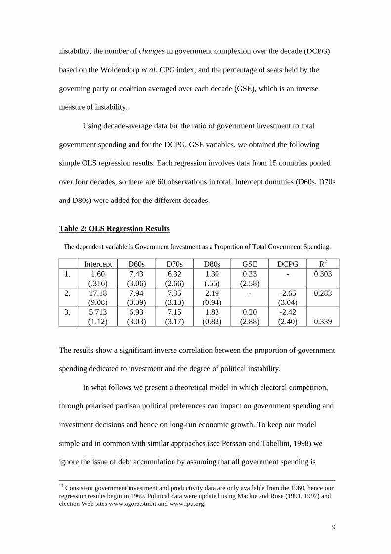
Using decade-average data for the ratio of government investment to total
government spending and for the DCPG, GSE variables, we obtained the following
simple OLS regression results. Each regression involves data from 15 countries pooled
over four decades, so there are 60 observations in total. Intercept dummies (D60s, D70s
and D80s) were added for the different decades.
Table 2: OLS Regression Results
The dependent variable is Government Investment as a Proportion of Total Government Spending.
Intercept D60s D70s D80s GSE DCPG R2
1. 1.60(.316)
7.43(3.06)
6.32(2.66)
1.30(.55)
0.23(2.58)
- 0.303
2. 17.18(9.08)
7.94(3.39)
7.35(3.13)
2.19(0.94)
- -2.65(3.04)
0.283
3. 5.713(1.12)
6.93(3.03)
7.15(3.17)
1.83(0.82)
0.20(2.88)
-2.42(2.40) 0.339
The results show a significant inverse correlation between the proportion of government
spending dedicated to investment and the degree of political instability.
In what follows we present a theoretical model in which electoral competition,
through polarised partisan political preferences can impact on government spending and
investment decisions and hence on long-run economic growth. To keep our model
simple and in common with similar approaches (see Persson and Tabellini, 1998) we
ignore the issue of debt accumulation by assuming that all government spending is
11 Consistent government investment and productivity data are only available from the 1960, hence ourregression results begin in 1960. Political data were updated using Mackie and Rose (1991, 1997) andelection Web sites www.agora.stm.it and www.ipu.org.

10
financed from current taxation12. What our model explains is how and when an increase
in political uncertainty may impact negatively on economic growth, and how partisan
preferences may affect the efficiency of the economic outcome in terms of the median
voter. As we shall see, the model provides an explanation for the link between political
uncertainty, the increase in the share of government consumption in overall fiscal
spending, and slower growth.
3. A Theoretical Model.
Our model is a simple model with government spending and endogenous
growth. The government is assumed to tax the final output of producers. Tax revenues
are then allocated between government consumption (which increases the current utility
of consumers), and government investment, which encourages future growth and
benefits consumers in the future. The tax rate and the allocation of government
spending between public consumption and investment is determined at each point in
time by the incumbent government.
Consumers in the economy are assumed to differ in their rate of time preference,
with some consumers benefiting more than others from future consumption13.
Consumers’ political attitudes are captured by their rate of time preference: more
patient consumers prefer higher tax rates and the allocation of a larger fraction of tax
revenues to government investment.
We assume a standard partisan-type political economy model, in which there are
two political parties, whose preferences are exogenously given at the outset. Each
12 The presence or absence of debt only matters in models in which there are non-Ricardian effects,which is not the case here.13 In a richer model one might want to explain the source of these differences in consumers’ timepreference. These might arise because of the presence or absence of intergenerational links in a model

11
party’s political platform is given by the rate of time preference at which future benefits
are capitalised. Consumers will vote for the party which most closely represents its
views, and, by assuming a majoritarian political system, the elected party will enact its
preferred policies. As in all standard partisan political models, we have to introduce an
element of political uncertainty, which we do by assuming that the median voter’s time
preference fluctuates over time14.
Before outlining and analysing our model, we summarise the key results which
emerge. First, the presence of political uncertainty creates policy myopia. Compared
with consumers who share the identical rate of time preference, political parties always
adopt policies which give rise to lower growth and a higher fraction of revenues spent
on public consumption. Second, a higher degree of political uncertainty has both
negative and positive effects on the growth rate (via the tax policies chosen by the
political parties). However, the net effect of increased political uncertainty is that it
discourages growth and increases the share of government consumption. Third, given
the distribution of consumer preferences, we can assess the economic efficiency of the
decisions made by the political parties. When compared to the median voter’s
preferences, the resulting equilibrium is generally inefficient. It turns out that the
economy may grow too fast or too slowly, and the fraction of expenditures allocated to
public consumption may be too high or too low.
with overlapping generations as opposed to infinitely-lived consumers (as assumed here). But, as longas there is some political uncertainty in the model, our conclusions would still hold.14 As in standard models, this can be either due to random voter turnout, or to shifts in the compositionand preference distribution of the electorate (see Alesina and Rosenthal, 1995).

12
3.1 The Production and Government Sectors
We assume a continuous-time15 model, in which the final output sector is perfectly
competitive and there is no private capital16. The aggregate production function is:
Y A L G Dt t t= −( ) ( )α α1 (1)
where Yt is final output (a numeraire), L is the working population (which we normalise
to one), D is ‘land’, which is equally owned by consumers and is again normalised to
one. Productivity is augmented through the variable At , which captures a learning-by-
doing effect, and through the flow of public investment, Gt (where we assume that
there is no congestion).
The government taxes final output at a rate 0 1< <τ , and the first order
conditions are:
w A xt t t= − −( )1 1τ α α (2)
q A xt t t= − − −( )( )1 1 1τ α α (3)
where x G At t t= ( / ) , w is the wage rate and q is the rental rate of land.
The variable At captures an external learning-by-doing effect. In line with
standard endogenous growth models, we assume that At is proportional to the
accumulation of output production per worker:
A b Y dst s
t= z0 (4)
where b>0 is the degree of the learning-by-doing effect. From (4), using (1) we have:
&A
A
bY
Abx
t tt
FHG
IKJ = F
HGIKJ = −1 α (5)
15 This turns out to be a convenient way to derive the growth equilibrium conditions in an infinite-horizon model. As we shall see below, this involves us modelling government changes as a Markovprocess. However, it turns out that it changes in the degree of political uncertainty can be modelledquite easily in a continuous-time context.16 This assumption is not particularly restrictive and is common to many endogenous growth models.
13
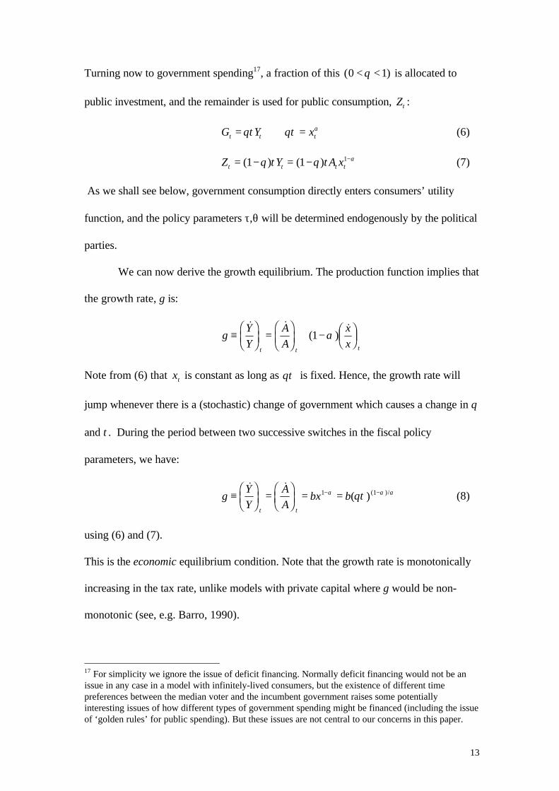
Turning now to government spending17, a fraction of this ( )0 1< <θ is allocated to
public investment, and the remainder is used for public consumption, Zt :
G Y xt t t= ⇒ =θτ θτ α (6)
Z Y A xt t t t= − = − −( ) ( )1 1 1θ τ θ τ α (7)
As we shall see below, government consumption directly enters consumers’ utility
function, and the policy parameters τ,θ will be determined endogenously by the political
parties.
We can now derive the growth equilibrium. The production function implies that
the growth rate, g is:
gY
Y
A
A
x
xt t t
≡FHG
IKJ =
FHG
IKJ + − F
HGIKJ
& &( )
&1 α
Note from (6) that xt is constant as long as θτ is fixed. Hence, the growth rate will
jump whenever there is a (stochastic) change of government which causes a change in θ
and τ. During the period between two successive switches in the fiscal policy
parameters, we have:
gY
Y
A
Abx b
t t
≡FHG
IKJ =
FHG
IKJ = =− −
& &( ) ( )/1 1α α αθτ (8)
using (6) and (7).
This is the economic equilibrium condition. Note that the growth rate is monotonically
increasing in the tax rate, unlike models with private capital where g would be non-
monotonic (see, e.g. Barro, 1990).
17 For simplicity we ignore the issue of deficit financing. Normally deficit financing would not be anissue in any case in a model with infinitely-lived consumers, but the existence of different timepreferences between the median voter and the incumbent government raises some potentiallyinteresting issues of how different types of government spending might be financed (including the issueof ‘golden rules’ for public spending). But these issues are not central to our concerns in this paper.

14
3.2 Voters Preferences and Behaviour
As noted earlier, we assume that consumers are infinitely lived, and differ in their rate of
subjective time preference, ρ. This parameter summarises their political preferences:
consumers with a lower value of ρ give greater weight to future consumption and
therefore tend to support a growth-oriented party. We assume that the distribution of
preferences is such that ρ ρ ρ∈[ , ] and ρ ρ ρ< < is continuously distributed with the
distribution function F(.).
The consumers’ intertemporal and instantaneous utility functions are given by:
U e u c Z ds
u c Z c Z
ts t
s st
s s s s
=
=
− −∞
−
z ρ
β β
( ) ( , )
( , ) 1(9)
where cs is the consumption of final output and Zs is the consumption of government
services. As there is no capital, consumers will spend their disposable income in each
instant on private consumption, i.e.:
c w q A xt t t t t= + = − −( )1 1τ α (10)
Note that (7) and (10) can be rewritten as:
c At t= − −α τ θτ α α( )( )( )/1 1 (11)
Z At t= − −( ) ( )( ) /1 1θ τ θτ α α (12)
Note that taxation reduces private consumption and boosts public consumption for a
given value of At . A higher tax rate will boost both types of consumption through its
positive impact on public investment (captured by the factor ( ) /τ α α1− ). Note also that
private consumption for all consumers is maximised at τ α= −1 . However, consumers
are not only interested in current consumption, and as a higher tax rate implies a higher

15
growth rate, consumers generally prefer a higher tax rate than (1-α), with the ideal tax
rate higher for the more patient consumers (i.e. those with a lower ρ).
As we shall see below, different political parties differ in their fiscal policies.
Consumers will generally vote for the party whose policy yields the highest utility. We
begin by characterising each consumers ideal policies τ and θ (and hence g). As we are
dealing with an infinite-horizon model, when consumers vote, they are fully committed
to the policy of their chosen party (i.e. they compare their level of utility under both
parties assuming that the policy will remain in place for an infinite horizon). Substituting
(11) and (12) into (9), and re-expressing the resulting equation using (8):
U gA g b g b
gtt( , , )( ) [ ( / ) ]( / )/
ρ ττ τ
ρ
β α α
=− −
−
−1 1
(13)
where we assume that ρ > g . By differentiating (13) we obtain the optimal fiscal policy
for the consumer, given his/her value of ρ. (Note that from (8), knowing the optimal
value of g, one can find the optimal value of θ, given τ). This illustrates the various
trade-offs faced by consumers. The optimal values of τ and g (and hence θ) are
determined implicitly by:
∂∂τ
τ β βα αUg bt = = + −−0 11: ( / ) ( )/ (14)
∂∂
βαα
τ ρ τα α α α
U
g
g
bg g
g
bt = +L
NMOQPFHG
IKJ −
RS|T|UV|W|
− = − FHG
IKJ
LNMM
OQPP
− −
0 11 1
: ( )/ ( ) /( )
(1- )1-
(15)
Equation (14) shows that as the tax rate increases private consumption falls due to the
distortionary tax effect and this has a negative impact on utility, but public consumption
increases due to higher tax revenues, which positively affects utility. The positive
relationship between the tax rate and growth in (14) is due to the fact that with a greater
proportion of resources dedicated to public investment (and higher growth), consumers
16
are more willing to endure higher taxes. Equation (15) shows that as the growth rate
rises the level effect of higher public investment on output raises private consumption
and current utility, whilst future utility increases because of the prospective rise in future
private and public consumption. However, less is spent on public consumption and this
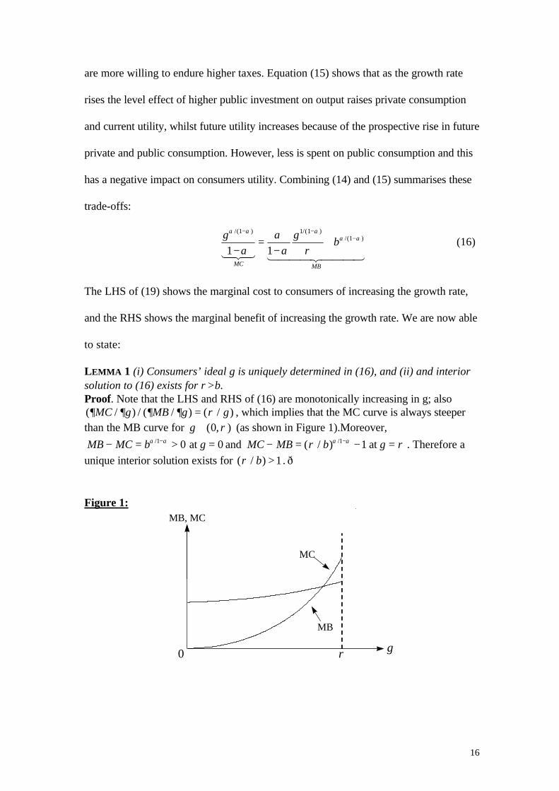
has a negative impact on consumers utility. Combining (14) and (15) summarises these
trade-offs:
g gb
MC MB
α α αα α
αα
α ρ
/( ) /( )/( )
1 1 11
1 1
− −−
−=
−+
124 34 1 2444 3444
(16)
The LHS of (19) shows the marginal cost to consumers of increasing the growth rate,
and the RHS shows the marginal benefit of increasing the growth rate. We are now able
to state:
LEMMA 1 (i) Consumers’ ideal g is uniquely determined in (16), and (ii) and interiorsolution to (16) exists for ρ>b.Proof. Note that the LHS and RHS of (16) are monotonically increasing in g; also( / ) / ( / ) ( / )∂ ∂ ∂ ∂ ρMC g MB g g= , which implies that the MC curve is always steeperthan the MB curve for g ∈( , )0 ρ (as shown in Figure 1).Moreover,
MB MC b g− = > =−α α/1 0 0 at and MC MB b g− = − =−( / ) /ρ ρα α1 1 at . Therefore a
unique interior solution exists for ( / )ρ b > 1. ð
Figure 1:
MC
MB
g
MB, MC
ρ0
17
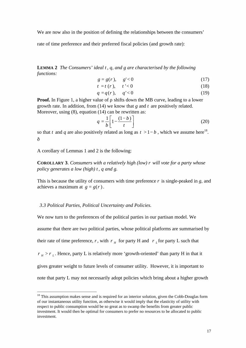
We are now also in the position of defining the relationships between the consumers’
rate of time preference and their preferred fiscal policies (and growth rate):
LEMMA 2 The Consumers’ ideal τ, θ, and g are characterised by the followingfunctions:
g g g= <( ), 'ρ 0 (17)τ τ ρ τ= <( ), ' 0 (18)θ θ ρ θ= <( ), ' 0 (19)
Proof. In Figure 1, a higher value of ρ shifts down the MB curve, leading to a lowergrowth rate. In addition, from (14) we know that g and τ are positively related.Moreover, using (8), equation (14) can be rewritten as:
θβ
βτ
= −−L
NMOQP
11
1( ) (20)
so that τ and θ are also positively related as long as τ β> −1 , which we assume here18.
ð
A corollary of Lemmas 1 and 2 is the following:
COROLLARY 3. Consumers with a relatively high (low) ρ will vote for a party whosepolicy generates a low (high) τ, θ and g.
This is because the utility of consumers with time preference ρ is single-peaked in g, andachieves a maximum at g g= ( )ρ .
3.3 Political Parties, Political Uncertainty and Policies.
We now turn to the preferences of the political parties in our partisan model. We
assume that there are two political parties, whose political platforms are summarised by
their rate of time preference, ρ, with ρ H for party H and ρ L for party L such that
ρ ρH L> . Hence, party L is relatively more ‘growth-oriented’ than party H in that it
gives greater weight to future levels of consumer utility. However, it is important to
note that party L may not necessarily adopt policies which bring about a higher growth
18 This assumption makes sense and is required for an interior solution, given the Cobb-Douglas formof our instantaneous utility function, as otherwise it would imply that the elasticity of utility withrespect to public consumption would be so great as to swamp the benefits from greater publicinvestment. It would then be optimal for consumers to prefer no resources to be allocated to publicinvestment.
18
rate in equilibrium. The policy outcomes will depend critically on the nature of the
political party’s utility function, which will depend on the role played by office
motivation, and hence by political uncertainty.
As explained above, we follow the standard political economy literature on
partisan models by assuming a majoritarian system, where the incumbent party has total
control on fiscal policy19. We will denote the two parties’ policies as
( , ), ,τ θi i i L H = , which will lead to outcome gi for growth. These policy outcomes
will of course be determined endogenously, as shown below. Taking the policy pairs
( , )τ θi i as given, consumers will decide whether to vote for party H or L.
To facilitate our analysis of voters’ behaviour we shall assume for the moment
that party H will deliver a lower growth rate than party L ( g gH L< ). The conditions
under which this will be the case will be derived formally below. In this case, it is
apparent that voters with a higher value of ρ will vote for party H and those with a
lower value of ρ will vote for party L. In what follows, let ~ρ denote the time preference
of the threshold voters, who are indifferent between supporting party H and party L
(i.e. the policies of both parties will yield them the same utility):
U Ut L L t H H(~, , ) (~, , )ρ τ θ ρ τ θ= (21)
Elections are assumed to take place at each instant20, t. As in standard partisan political
economy models, political uncertainty derives from stochastic fluctuations in the voters’
distribution function F( )ρ , either because of random voter turnout, or variations in the
composition of the voting population. Hence an incumbent political party faces the risk
19 One potential extension of our model, which we do not explore here for reasons of space, is that theminority party may also have some control on fiscal policy through a bargaining framework (see forexample Rogoff, 1990).20 As noted previously our conclusions would not be affected by considering a discrete-time version ofthe model in which elections are held in every period. Our continuous-time set-up merely makes theanalysis of our endogenous-growth model easier.
19
of being replaced by the opposition party. More specifically, we assume that at any
point in time the distribution function takes the following two functional forms:
FF
Fl
h
( )( )
( )ρ
ρρ
=RST
Next, let ρ ρl h and denote the rates of time preference of the median voters associated
with each distribution function, i.e. F Fl l h h( ) ( ) /ρ ρ= = 1 2 . The only condition which
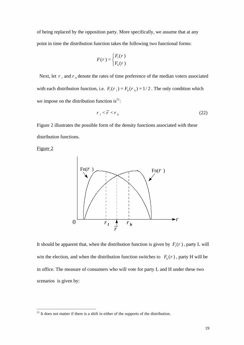
we impose on the distribution function is21:
ρ ρ ρl h< <~ (22)
Figure 2 illustrates the possible form of the density functions associated with these
distribution functions.
Figure 2
Fn(ρ )
ρ0
Fn(ρ )
ρl ρh~ρ
It should be apparent that, when the distribution function is given by Fl ( )ρ , party L will
win the election, and when the distribution function switches to Fh ( )ρ , party H will be
in office. The measure of consumers who will vote for party L and H under these two
scenarios is given by:
21 It does not matter if there is a shift in either of the supports of the distribution.
20
N F F
N F FL l l l
H h h h
= > == − > − =
(~) ( ) /
(~) ( ) /
ρ ρρ ρ
1 2
1 1 1 2
The degree of political uncertainty can be modelled by assuming that the stochastic
change between the two distribution functions follows a Markov process, i.e.:
F F
F Fl h
h l
( ) ( )
( ) ( )
ρ ρ ηρ ρ λ
→→
with a flow probability
with a flow probability
Note that by setting η λ= we have a similar situation to one in discrete time where
both parties have an equal chance of being elected. An increase in these flow
probabilities will increase the degree of political uncertainty because it will lead to a
greater number of government changes.
Next we turn our attention on the incentives faced by each party i in deciding on
its policy set. We assume that each party maximises the sum of the utility functions of
the consumers who support it, i.e. the instantaneous pay-off is N u c Zi ( , ) . However, we
also assume that each party is office-motivated, in that it gains a zero pay-off when it is
out of office22. We can now write down the Bellman equations for each party i:
V A N u c Z dt dt V A gAdt p dt V A gAdt p dtig
i i i i i i( ) max ( , ) ( ) ( )( ) $ ( ),
= + − + − + +τ
ρ1 1o t (23)
where V Ai t( ) is the value function which party i achieves when it is in office, and
$ ( )V Ai t when it is out of office, and pi is defined as the flow probability of losing the
current election (i.e. p pL H= =η λ, ). Note from (26) that the state variable is A, so
that when a party is elected, it gains utility N u c Zi ( , ) during interval dt. But during this
22 There are different ways of introducing office motivation in a political party’s pay-off function (seeRogoff, 1990, Persson and Tabellini, 1990, 1998). In models where elections have a disciplining effecton incumbent governments one can introduce office motivation as a fixed benefit from being in office,or fixed cost from being out of office. But our purpose here is to show how policy myopia can arise in apartisan model, and policy myopia effects will emerge as long as the political benefits to a party frombeing in office are related to the policy actions taken. Thus, for instance, our results would still hold ina model where each party derives some benefit when it is out of office from the policies undertaken, aslong as the benefits when in office depend in some measure on the utility of the consumers who elected

21
time interval, the technological level of the economy will have improved by gAdt ,
which enters the value function at the end of the time interval. At that time, party i will
still be in office with a probability of ( )1− p dti , achieving V A gAdti ( )+ , or will lose
the election with a complementary probability p dti , attaining $ ( )V A gAdti + .
Of course, unlike a two-period model, in our infinite-horizon model a party
which loses office may always expect to return to office at some future date and its
current policies will therefore have an impact on future pay-offs even after losing an
election. This will therefore need to be taken into account in computing $ ( )V Ai , and the
stochastic steady-state equilibrium of the model. We can determine $ ( )V Ai by the
following recursive equation:
$ ( ) ( ) $ ( )( ) ( )V A dt V A gAdt q dt V A gAdt q dti i i i i i= − + − + +1 1ρ (24)
where qi is the flow probability of winning in the current election and is defined as
( , )q qL H= =λ η . From (24) we see that when party i is not in office, at the end of time
interval dt it will still not be elected with probability ( )1− q dti , attaining $Vi , or it will be
elected with a complementary probability q dti , attaining Vi .
In order to find the optimal fiscal policies by the two parties, we can
differentiate (23), holding $Vi as given. The first-order conditions are:
τ β βα α
iig
b= F
HGIKJ + −
−/1
1 (25)
′ =−
−FHG
IKJ
−
V AN
b
gi
i i( )/ψα
α α1
11 (26)
where i=H,L and ψ β ββ β≡ − −( )1 1 .
the government. Of course assuming a zero pay-off for each party when it is out of office involves aconsiderable gain in analytical simplicity.

22
We can compare (25) and (26), the chosen policies of the two parties with the
optimal tax and expenditure allocation (growth) policies from the point of view of
consumers with the same rate of time preference (equations (14) and (15)). Whilst (25)
is identical to (14), (26) differs from (16). This implies that the fiscal policies of each
political party does not match those of consumers with the same political stance as the
two parties. We shall return to this point below.
3.4 The Stochastic Steady State Growth Equilibrium under Political Uncertainty
Having characterised the policy choices of each political party, and the working of our
endogenous growth model, we are now in a position to solve for the stochastic steady-
state equilibrium of our model.
We know that in equilibrium:
V A V A i H Li io( ) ,= = (27)
So that (26) now becomes:
VN
b
gio i i=
−−
FHG
IKJ
−ψα
α α/1
11 (28)
Letting dt → 0 in the Bellman equations (23) and (24) and rewriting the resulting
equations with (27) and (28), we obtain the stochastic steady-state growth equilibrium
under the two regimes (G):
g g
gbi
MC
i
i i i
MB
α α αα α
αα
α ρ
/( ) / ( )/( )
( )
1 1 11
1 1
− −−
−=
− ++
124 34 1 24444 34444Γ
(G)
where Γ ΓL LL L
L LH H
H H
H H
gg
gg
g
g( )
( ), ( )
( )=
−+ −
=−
+ −η ρλ ρ
λ ρη ρ
(G’)
This expression shows the marginal costs and benefits to each party of increasing the
growth rate, and exactly parallels equation (16), which showed the voters’ preferred

23
growth rate. It can be readily seen that, unlike the consumers’ ideal choice for g, the
political parties’ decision is affected by the presence of the extra term Γi ig( ) : these
capture the effect of policy uncertainty which generates a degree of policy myopia.
Before discussing the policy myopia effect in detail, we first have to establish the
following proposition:
PROPOSITION 4 (i) The growth rate generated by party i’s fiscal policies is uniquelydetermined in (G) and (ii) and interior solution to (G) exists for ρ>b.Proof. Note that ′ <Γi g( ) 0 , so that the MB curve is monotonically increasing ing ∈( , )0 ρ . In addition, Γi g g( ) ( , )> ∈0 0 for ρ and Γi g g g( ) = = =0 0 at and ρ .Hence, the MB curve associated with (G) is located entirely below the MB curve in(16), except for g g= =0 and ρ where they coincide. Hence, as shown in Figure 3, a
unique interior solution exists for ρ > b . ð
Figure 3:
MC
g
MB, MC
ρ0
MBv
0
MBi
where MBi represents the marginal benefit to party i and
MBv represents the marginal benefit to a voter with the same ρ as party i.
The policy myopia effect is due to the presence of political uncertainty, which
means that the political parties have an uncertainty-adjusted discount rate,
ρ i i g+ Γ ( ) which is higher compared to consumers with the same rate of time
preference. That the growth rate chosen by party i is not identical to the ideal g chosen

24
by consumers who share the same political preferences is apparent from Figure 3. The
knowledge that party i will lose office at some stage in the future creates this short-
sightedness in policy. As the MB of party i is always below that of consumers, the
party’s fiscal policy will be biased towards government consumption and against
growth. This can be summarised as the following proposition:
PROPOSITION 5 Political parties always set policies such that taxes are lower and thefraction of tax revenue spent on public consumption is higher than consumers with theidentical rate of time preference.
The magnitude of the bias against growth-oriented fiscal policies caused by policy
myopia obviously depends on the degree of political uncertainty. A higher value of pi ,
the flow probability of losing office increases the myopia term, Γi , and hence the
effective discount rate of the government. Interestingly, although a higher value of qi ,
the flow probability of winning the next election after losing the current one tends to
lower the value of Γi , as one might expect, it cannot eliminate the policy myopia effect.
The effect only disappears as qi → ∞ .
This begs the question of what the net effect will be on the average growth rate
of changing the degree of political uncertainty, which is one of the key issues we wanted
to address. A higher flow probability of the current incumbent losing the next election
( pi ), and a higher flow probability of party i losing the next election given that it is not
the current incumbent ( qi ) may both be seen as increasing political uncertainty but, as
noted above, they have opposing impacts on the growth rate. Which effect dominates?
The most sensible way to address this is by setting p p qi i≡ = = =λ η , so that an
increase in political uncertainty is not biased against a particular party (parties alternate
in power more frequently, with neither party increasing its average share of time in
office). Now each party has an equal chance of winning each election with the same

25
flow probability. In these circumstances, it is straightforward to show that Γi ig( ) rises
as p increases, so that the negative effect of political uncertainty on growth dominates.
In this instance current fiscal policy is determined by the prospects of the outcome in the
immediate election, and the prospect of being re-elected after losing is too distant in the
future to matter significantly.
It is intuitively obvious that the average growth rate in the economy will also fall
as political uncertainty increases. As party L is in office with a flow probability of λ and
party H replaces it with a flow probability of η, the average growth rate in the economy
is given by:
g g gL H= + −Λ Λ Λ( )1 , = / ( + )λ λ η (29)
Again, as above, we want to consider an increase in political uncertainty, p, where
p ≡ =λ η . The average growth rate then becomes g g gL H= +( ) / 2 . We have already
shown that a higher p raises the policy myopia term Γi ig( ) , shifting the MB curve down
with a lower g. Thus, the average growth rate unambiguously falls.
3.5 Economic Efficiency
Having established that greater political uncertainty leads to increased policy myopia
and to lower growth, we also have to consider whether the steady-state stochastic
political equilibrium described above is inefficient in terms of consumer welfare. We
have already established that growth is lower than would be preferred by each party’s
natural constituency of voters.
With different preferences between consumers the issue has to be confronted as
to what we mean by an ‘efficient outcome’. The most natural metric to use is that of the

26
median voter23. Suppose the median voter could choose a policy pair ( , )τ θ . What
equilibrium would emerge compared to the equilibrium discussed so far in (G)?
To do this we have to compare the outcome in (G) with that which would
prevail in a world where the median voter could determine their ideal fiscal policy. Of
course in our model we assume that the median voter’s time preference stochastically
fluctuates between ρ ρl h and . The key issue is what drives these fluctuations. The
trivial case is where these fluctuations are due purely to random voter turnout, and
preferences remain unchanged in the underlying population, as the growth rate chosen
by the two parties as they alternate in power will oscillate around the level which
corresponds to that preferred by the median voter. However, if there are fluctuations in
the preferences of the population as one might expect there to be over time, due to
changes in demographic composition24, then with static political preferences in the two
parties the issue of economic efficiency requires closer attention.
In this case fluctuations in the median voter’s time preference will lead to
fluctuations over time in the growth rate which they would prefer. From equation (16)
this would be given by:
g gb j h lj j
j
α α αα α
αα
α ρ
/ // ,
1 1 11
1 1
− −−
−=
−+ =, (30)
The average growth rate is:
g g gml h= + −Λ Λ( )1 (31)
Equations (29) and (30) imply:
23 See Muscatelli (1998) for an example of a model where the economic efficiency of different regimesis evaluated with distributed preferences in a partisan model of monetary policy.24 Family composition and inter-generational utility linkages may also matter here. For instance, onemight have expected voters in many Western economies in the 1950s and early 1960s after the post-war baby boom to be more interested in public investment and future growth than voters in the 1980sand 1990s, with the decline in population growth. These issues however would need to be addressed ina different model with overlapping generations.
27
g g g g g gml L h H− = − + − −Λ Λ( ) ( )( )1 (32)
This allows us to state the following proposition and corollary:
PROPOSITION 6 The political party equilibrium is generally inefficient, and the growthrate may be too high or too low compared to the preferred median voter outcome, i.e.g gm ≠ .Proof. First note that the growth rate crucially depends on the discount rate that themedian voter and the political parties use (see (G) and (30)). Thus, whetherg g g gl L h H> < > <or and or depends on the values ofρ ρj i ij l h g i H L , and = + =, ( ), ,Γ . There are four possible cases:
1. ρ ρ ρ ρL L L l h H H H L l h Hmg g g g g g g or g+ < < < + ⇒ > > > ⇒ < >Γ Γ( ) ( )
2. ρ ρ ρ ρl L L L H H H h l L H hmg g g g g g g or g< + < + < ⇒ > > > ⇒ < >Γ Γ( ) ( )
3. ρ ρ ρ ρl L L L h H H H l L h Hmg g g g g g g g< + < < + ⇒ > > > ⇒ >Γ Γ( ) ( )
4. ρ ρ ρ ρL L L l H H H h L l H hmg g g g g g g g+ < < + < ⇒ > > > ⇒ <Γ Γ( ) ( ) . ð
COROLLARY 7 The fiscal policies in these four cases are:• Cases (1) and (2): τ τ θ θm mor or> < > < and • Case (3): τ τ θ θm m> > and • Case (4): τ τ θ θm m< < and Proof These results follow directly from proposition 6 and (14) and (20). ð
Essentially the relationship between the outcome in the political equilibrium and the
ideal outcome for the median voter depends on the positioning of the two political
parties (which is exogenous in our model) relative to the fluctuating preferences of the
median voter. Hence the outcome depends critically on the polarisation of political
party preferences, and the swing in voters’ political attitudes. This can be readily seen
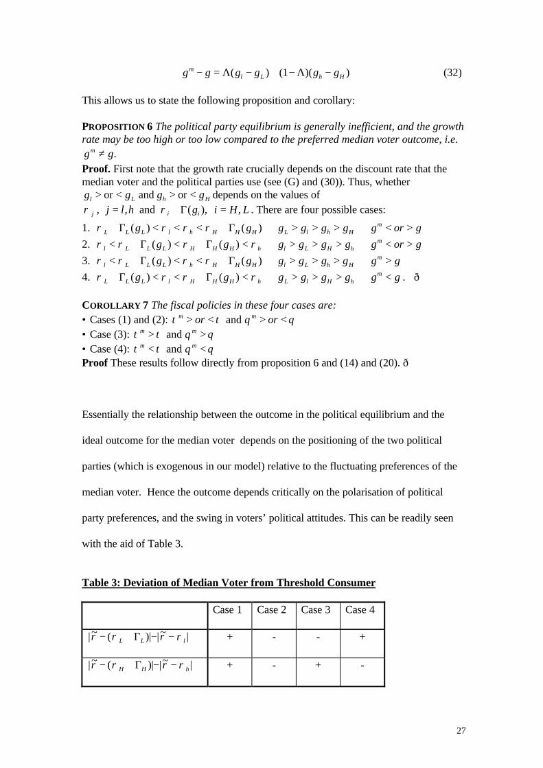
with the aid of Table 3.
Table 3: Deviation of Median Voter from Threshold Consumer
Case 1 Case 2 Case 3 Case 4
|~ ( )| |~ |ρ ρ ρ ρ− + − −L L lΓ + - - +
|~ ( )| |~ |ρ ρ ρ ρ− + − −H H hΓ + - + -
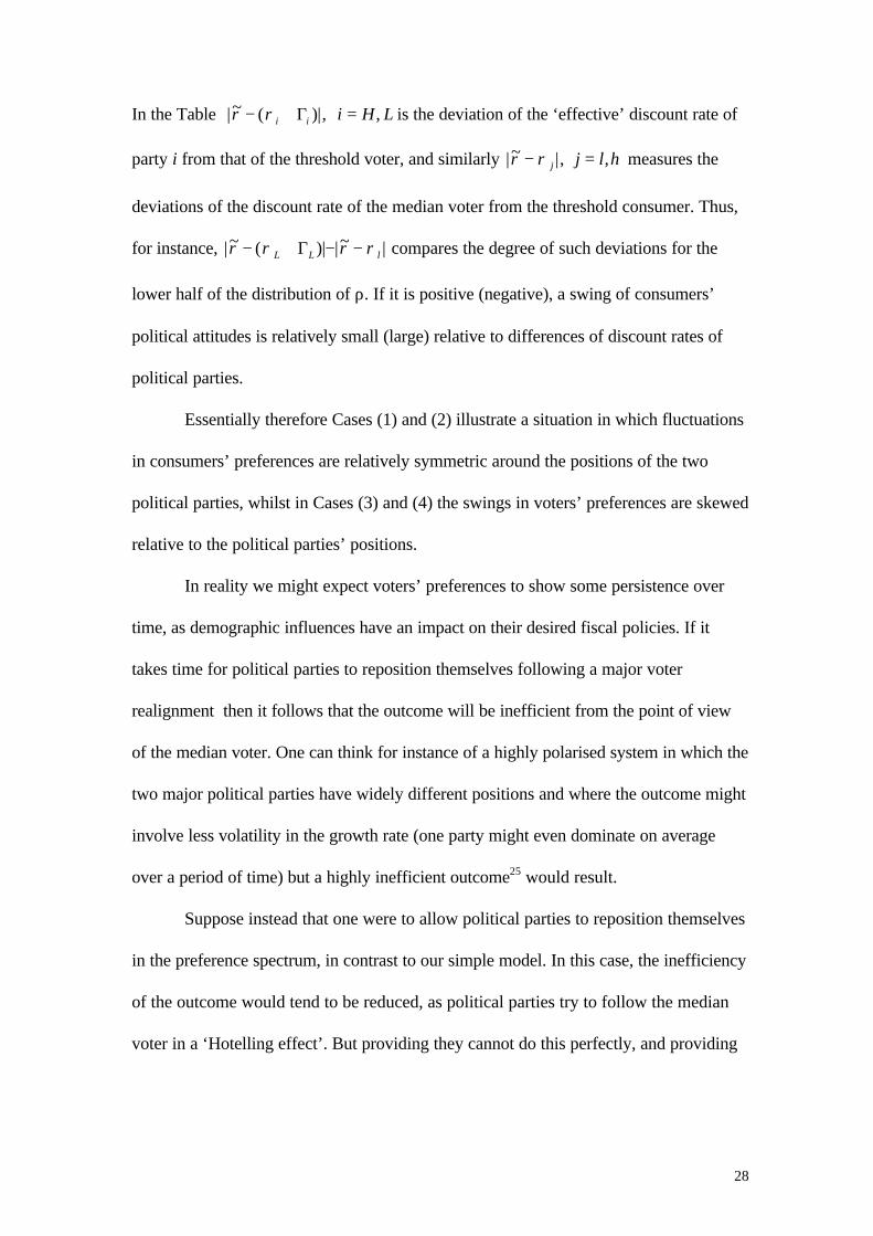
28
In the Table |~ ( )|, ,ρ ρ− + =i i i H LΓ is the deviation of the ‘effective’ discount rate of
party i from that of the threshold voter, and similarly |~ |, ,ρ ρ− =j j l h measures the
deviations of the discount rate of the median voter from the threshold consumer. Thus,
for instance, |~ ( )| |~ |ρ ρ ρ ρ− + − −L L lΓ compares the degree of such deviations for the
lower half of the distribution of ρ. If it is positive (negative), a swing of consumers’
political attitudes is relatively small (large) relative to differences of discount rates of
political parties.
Essentially therefore Cases (1) and (2) illustrate a situation in which fluctuations
in consumers’ preferences are relatively symmetric around the positions of the two
political parties, whilst in Cases (3) and (4) the swings in voters’ preferences are skewed
relative to the political parties’ positions.
In reality we might expect voters’ preferences to show some persistence over
time, as demographic influences have an impact on their desired fiscal policies. If it
takes time for political parties to reposition themselves following a major voter
realignment then it follows that the outcome will be inefficient from the point of view
of the median voter. One can think for instance of a highly polarised system in which the
two major political parties have widely different positions and where the outcome might
involve less volatility in the growth rate (one party might even dominate on average
over a period of time) but a highly inefficient outcome25 would result.
Suppose instead that one were to allow political parties to reposition themselves
in the preference spectrum, in contrast to our simple model. In this case, the inefficiency
of the outcome would tend to be reduced, as political parties try to follow the median
voter in a ‘Hotelling effect’. But providing they cannot do this perfectly, and providing
29
some degree of political uncertainty remains, the policy myopia effect would still persist,
and we would still expect a higher degree of uncertainty to reduce public investment
and growth in equilibrium.
Before concluding, we need to address the assumption made so far that that
party H will deliver a lower growth rate than party L ( g gH L< ). We will derive the
condition under which this inequality will hold and consider what happens if it does not
hold.
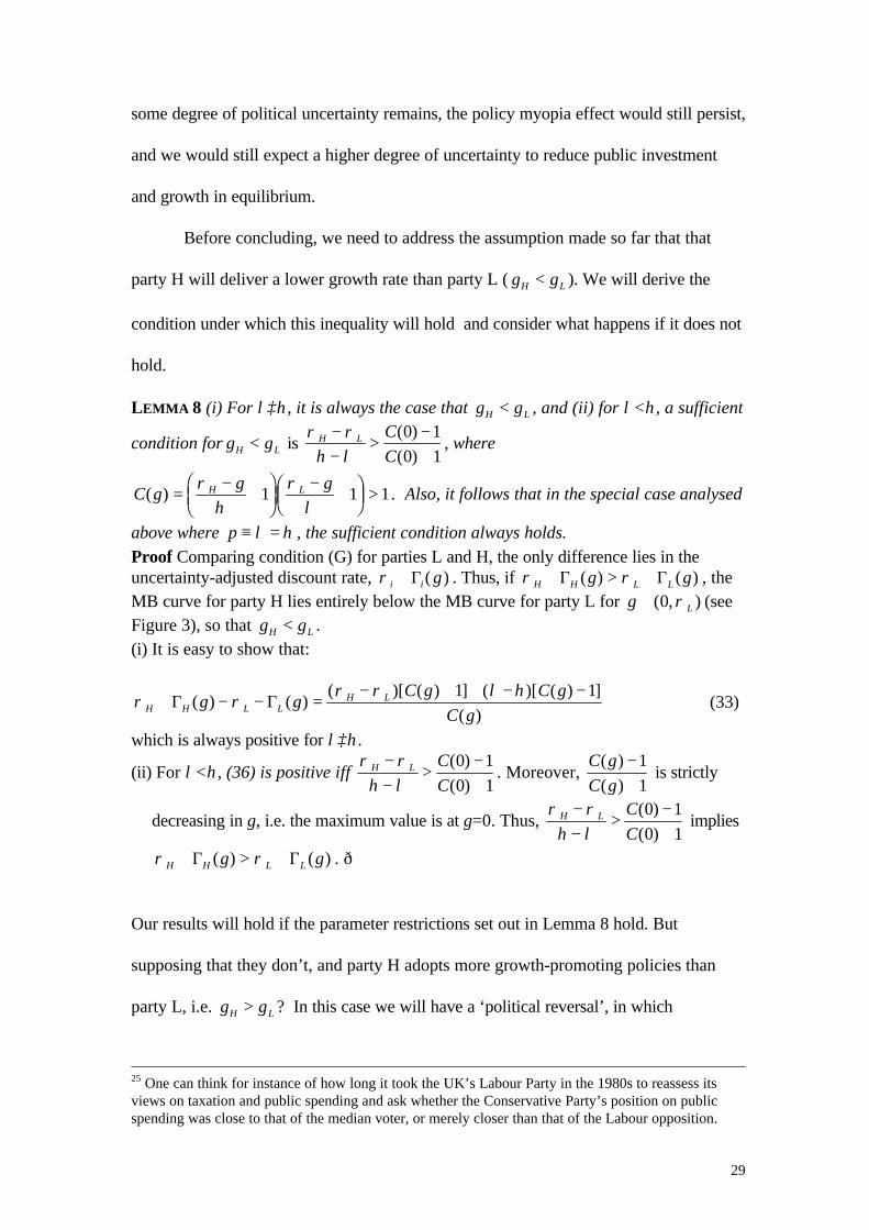
LEMMA 8 (i) For λ≥η, it is always the case that g gH L< , and (ii) for λ<η, a sufficient
condition for g gH L< is ρ ρ
η λH L C
C
−−
>−+
( )
( )
0 1
0 1, where
C gg gH L( ) =
−+
FHG
IKJ
−+F
HGIKJ >
ρη
ρλ
1 1 1 . Also, it follows that in the special case analysed
above where p ≡ =λ η , the sufficient condition always holds.
Proof Comparing condition (G) for parties L and H, the only difference lies in theuncertainty-adjusted discount rate, ρ i i g+ Γ ( ) . Thus, if ρ ρH H L Lg g+ > +Γ Γ( ) ( ) , theMB curve for party H lies entirely below the MB curve for party L for g L∈( , )0 ρ (seeFigure 3), so that g gH L< .(i) It is easy to show that:
ρ ρρ ρ λ η
H H L LH Lg g
C g C g
C g+ − − =
− + + − −Γ Γ( ) ( )
( )[ ( ) ] ( )[ ( ) ]
( )
1 1(33)
which is always positive for λ≥η.
(ii) For λ<η, (36) is positive iff ρ ρ
η λH L C
C
−−
>−+
( )
( )
0 1
0 1. Moreover,
C g
C g
( )
( )
−+
1
1 is strictly
decreasing in g, i.e. the maximum value is at g=0. Thus, ρ ρ
η λH L C
C
−−
>−+
( )
( )
0 1
0 1 implies
ρ ρH H L Lg g+ > +Γ Γ( ) ( ) . ð
Our results will hold if the parameter restrictions set out in Lemma 8 hold. But
supposing that they don’t, and party H adopts more growth-promoting policies than
party L, i.e. g gH L> ? In this case we will have a ‘political reversal’, in which
25 One can think for instance of how long it took the UK’s Labour Party in the 1980s to reassess itsviews on taxation and public spending and ask whether the Conservative Party’s position on publicspending was close to that of the median voter, or merely closer than that of the Labour opposition.

30
consumers with a lower (higher) ρ will vote for party H (L), and party L will be elected
whenever the distribution function of voters is given by Fh ( )ρ , whilst party H will be
elected when the distribution function is Fl ( )ρ . Apart from this, equilibrium condition
(G) remains the same, except that in (G’) λ and η will be interchanged.
Essentially, if the party preferences and other model parameters are such that
there is a ‘political reversal’, the party which is more growth-oriented (L) will actually
adopt a less growth-oriented strategy than party H, due to the different degrees of
political uncertainty faced by the two parties, i.e. due to L’s lower prospects of being
re-elected compared to H. As long as both party’s have an equal probability of being in
office (i.e. p ≡ =λ η ), political reversals cannot occur as the two party’s relative
political preferences will dominate their relative policy stance. Thus, to summarise, all
our results on policy myopia and the effect of policy uncertainty on fiscal policy still
hold, even in this special case, but with a further twist regarding the two political
parties’ relative policy stance.
4. Conclusions.
This paper has argued that there is a significant link between increased political
instability, reduced public investment and lower productivity growth in the OECD
economies. Using political data and a panel for various countries over the period 1960-
98 we show that there is a strong correlation between increased political instability and
the reduction in government investment as a proportion of total fiscal spending.
We explain this observed correlation using a model of endogenous growth with
rational partisan policymakers. Our model shows that, with greater political uncertainty,
it is rational for policy myopia effects to set in and for incumbent politicians to reduce
31
public spending and taxation, and to increase the share of government consumption in
total government spending. These effects remain, even if there is a prospect of a exit
from office and a subsequent return to power by the incumbent politician. From the
point of view of economic efficiency, a more significant result is that political parties
will adopt policy platforms with lower taxes and government investment spending than
their own constituency. Furthermore, the outcome will generally be inefficient from the
point of view of the median voter.
A number of extensions of this framework are possible and we intend to take
these up in future work. The first potential objection to our observed correlations is that
lower growth generates greater political instability. The impact of economic outcomes
and fiscal policy decisions on the popularity and survival of governments has been
recently analysed in Alesina et al. (1998), and we intend to perform some more formal
empirical work to jointly model the probability of survival of governments and their
fiscal decisions.
The second potential extension to our work is on the theoretical front. Our
model tends to ignore the role of government debt in ‘passing the buck’ to future
governments. The strategic role of government debt in this context has already been
analysed by previous authors (e.g. Milesi-Ferretti and Spolaore, 1994). Whilst it is
undoubtedly true that incumbents could use debt to constrain the choice of their
successors, introducing such effects into our model would create considerable analytical
complexities without producing any new results in this area. A more fruitful extension
would be to allow political party platforms to gravitate gradually over time, following
shifts in public opinion. For instance in a model with overlapping generations, one can
conceive of outcomes in which demographic shifts may cause movements in the median
voter’s preferences over time. At the same time, political party platforms and

32
polarisation will only evolve slowly because of the presence of interest groups (see
Alesina and Rosenthal, 1995). In these circumstances one might then be able to explain
changes in political polarisation and political platforms as functions of more
fundamental forces such as gradual demographic change in the industrialised economies.
References
Alesina, A. and Perotti, R. (1997). ‘Fiscal adjustments in OECD countries: compositionand macroeconomic effects.’ IMF Staff Papers, 44 (2), 210-48.
Alesina, A. and Perotti, R. (1996). ‘Reducing budget deficits.’ Swedish EconomicPolicy Review, 3(1), 113-34.
Alesina, A. and Rosenthal, H. (1995). Partisan Politics, Divided Government, and theEconomy.
Alesina, A. and Tabellini, G. (1990). ‘A positive theory of fiscal deficits and governmentdebt.’ Review of Economic Studies, 57, 403-14.
Alesina, A., Perotti, R. and Tavares, J. (1998). ‘The political economy of fiscaladjustments.’ Brookings Papers on Economic Activity, 1, 197-266
Alesina, A., Ozler, S., Roubini, N. and Swagel, P. (1996). Journal of EconomicGrowth, 1, 189-211.
Aschauer, D. (1989). ‘Is public expenditure productive?’ Journal of MonetaryEconomics, 23, 177-200.
Barro, R. (1990). ‘Government spending in a simple model of endogenous growth.’Journal of Political Economy, 98(5), S103-25.
Barro, R. (1996). ‘Democracy and growth.’ Journal of Economic Growth, 1, 1-27.
Benhabib, J. and Rustichini, A. (1996). ‘Social conflict and growth.’ Journal ofEconomic Growth, 1, 125-39.
Calvo, G. and Drazen, A. (1997). ‘Uncertain duration of reform: dynamic implications.’NBER Working Paper 5925.
Dalle Nogare, C. (1997) ‘Ideological Polarisation, Coalition Governments and Delays in
Stabilisation’ University of Glasgow Discussion Paper n.9710.
Devarajan, S., Swaroop, V. and Zou, H. (1996). ‘The composition of publicexpenditure and economic growth.’ Journal of Monetary Economics, 37, 313-44.
Devereux, M. and Wen, J.F. (1996). ‘Political uncertainty, capital taxation and growth.’Mimeo, University of British Columbia.
Easterly, W. and Rebelo, S. (1993). ‘Fiscal policy and economic growth: an empiricalinvestigation.’ Journal of Monetary Economics, 32, 417-58.

33
Giavazzi, F. and Pagano, M. (1990). ‘Can severe fiscal contractions be expansionary?Tales of two small European countries.’ NBER Macroeconomics Annual, 75-116. Giavazzi, F. and Pagano, M. (1995). ‘Non-Keynesian effects of fiscalpolicy changes: international evidence and the Swedish experience.’, NBERWorking Paper n.5332.
Grilli, V., Masciandaro, D. and Tabellini, G. (1991). ‘Political and monetary institutionsand public financial policies in the industrial countries.’ Economic Policy, 6,341-92.
Holtz-Eakin, D. and Schwartz, A.E. (1994). ‘Infrastructure in a structural model ofeconomic growth.’ NBER Working Paper n.4824.
Laakso and Taagepera (1979). ‘Effective Number of Parties: A Measure withApplication to Western Europe’, Comparative Political Studies 12.
Mackie, D. and Rose, R. (1997). ‘A Decade of Election Results: Updating theInternational Almanac’ Studies in Public Policy, Centre for Study of PublicPolicy, University of Strathclyde.
Mackie, D. and Rose. R. (1991). ‘The International Almanac of Electoral History’Third Edition, Macmillan, Hants.
Milesi-Ferretti, G.M. and Spolaore, E. (1994). ‘How cynical can an incumbent be?Strategic policy in a model of government spending.’ Journal of PublicEconomics, 55, 121-40.
Morrison, C. and Schwartz, A.E. (1992). ‘State infrastructure and productiveperformance.’ NBER Working Paper n.3981.
Munnell, A. (1990). ‘Why has productivity growth declined? Productivity and publicinvestment.’ New England Economic Review, Jan/Feb, 3-22.
Murphy, K., Shleifer, A. and Vishny, R.W. (1991). ‘The allocation of talent:implications for growth.’ Quarterly Journal of Economics, 106, 506-30.
Muscatelli, V.A. (1998). ‘Political consensus, uncertain preferences and central bankindependence.’, Oxford Economic Papers, 50, 412-30.
Perotti, R. (1993). ‘Political equilibrium, income distribution and growth.’ Review ofEconomic Studies, 60, 755-76.
Perotti, R. (1996). ‘Growth, income distribution and democracy: what the data say.’Journal of Economic Growth, 1, 149-88.
Persson, T. and Tabellini, G. (1990). Macroeconomic policy, credibility and politics,Harwood Academic Publishers, London.
Persson, T. and Tabellini, G. (1998). ‘Political Economics and Macroeconomic Policy.’forthcoming in J.Taylor and M. Woodford (eds.), Handbook ofMacroeconomics, Amsterdam: North-Holland.
Rodrik, D. (1991). ‘Policy uncertainty and private investment in developing countries.’Journal of Development Economics, 36, 227-49.
Rogoff, K. (1990). ‘Equilibrium political budget cycles.’ American Economic Review,80, 21-36.

34
Roubini, N. and Sachs, J. (1989a). ‘Political and economic determinants of budgetdeficits in the industrialised countries.’ European Economic Review, 33, 903-33.
Roubini, N. and Sachs, J. (1989b). ‘Government spending and budget deficits in theindustrialised countries.’ Economic Policy, 8, 99-132.
Saint-Paul, G. and Verdier, T. (1993). ‘Education, democracy and growth.’ Journal ofDevelopment Economics, 42, 399-407.
Svensson, J. (1993). ‘Investment, property rights and political instability: theory andevidence.’ European Economic Review, forthcoming.
Tornell, A. and Velasco, A. (1992). ‘The tragedy of the commons and economicgrowth: why does capital flow from poor to rich countries?’ Journal of PoliticalEconomy, 100, 1208-31.
Woldendorp, J., Keman, H. and Budge, I. (1993). ‘Political data 1945-90: Partygovernment in 20 democracies.’ European Journal of Political Research, 24(1), 1-120.

35
Table 2:
1960-69 1970-79 1980-89 1990-97
intercept 25.88 (15.75) 25.14 (9.44) 19.09 (6.51) 17.58 (5.35)DCPG -3.61 (-2.41) -3.08 (-2.00) -1.64 (-1.00) -3.03 (-1.28)R2 0.308 0.236 0.071 0.109intercept 10.96 (1.52) 4.73 (0.49) -0.49 (-0.04) 4.82 (12.44)GSE 0.20 (1.79) 0.28 (1.69) 0.29 (1.26) 0.17 (0.78)R2 0.188 0.180 0.109 0.055intercept 20.80 (2.28) 13.41 (1.16) 19.97 (1.7) 12.39 (0.93)TERM 0.03 (0.25) 0.09 (0.65) -0.05 (-0.34) 0.02 (0.14)R2 0.004 0.032 0.088 0.002intercept 27.12 (10.25) 25.25 (5.49) 13.39 (3.82) 6.52 (1.44)NTY -2.06 (-1.75) -1.90 (-1.04) 1.19 (0.88) 5.11 (1.91)R2 0.191 0.076 0.056 0.212


