
THE JAMES A. BAKER III INSTITUTE FOR PUBLIC POLICY
RICE UNIVERSITY
A MODEL OF THE
OPERATION AND DEVELOPMENT OF A
NATIONAL OIL COMPANY
BY
PETER HARTLEY RICE UNIVERSITY
KENNETH B. MEDLOCK III RICE UNIVERSITY
PREPARED IN CONJUNCTION WITH AN ENERGY STUDY SPONSORED BY THE JAMES A. BAKER III INSTITUTE FOR PUBLIC POLICY
AND JAPAN PETROLEUM ENERGY CENTER
RICE UNIVERSITY – MARCH 2007

THIS PAPER WAS WRITTEN BY A RESEARCHER (OR RESEARCHERS) WHO
PARTICIPATED IN THE JOINT BAKER INSTITUTE/JAPAN PETROLEUM ENERGY
CENTER POLICY REPORT, THE CHANGING ROLE OF NATIONAL OIL COMPANIES IN
INTERNATIONAL ENERGY MARKETS. WHEREVER FEASIBLE, THIS PAPER HAS BEEN
REVIEWED BY OUTSIDE EXPERTS BEFORE RELEASE. HOWEVER, THE RESEARCH AND
THE VIEWS EXPRESSED WITHIN ARE THOSE OF THE INDIVIDUAL RESEARCHER(S) AND DO NOT NECESSARILY REPRESENT THE VIEWS OF THE JAMES A. BAKER III
INSTITUTE FOR PUBLIC POLICY NOR THOSE OF THE JAPAN PETROLEUM ENERGY
CENTER.
© 2007 BY THE JAMES A. BAKER III INSTITUTE FOR PUBLIC POLICY OF RICE UNIVERSITY
THIS MATERIAL MAY BE QUOTED OR REPRODUCED WITHOUT PRIOR PERMISSION, PROVIDED APPROPRIATE CREDIT IS GIVEN TO THE AUTHOR AND
THE JAMES A. BAKER III INSTITUTE FOR PUBLIC POLICY

ABOUT THE POLICY REPORT
THE CHANGING ROLE OF NATIONAL OIL COMPANIES
IN INTERNATIONAL ENERGY MARKETS Of world proven oil reserves of 1,148 billion barrels, approximately 77% of these
resources are under the control of national oil companies (NOCs) with no equity
participation by foreign, international oil companies. The Western international oil
companies now control less than 10% of the world’s oil and gas resource base. In terms
of current world oil production, NOCs also dominate. Of the top 20 oil producing
companies in the world, 14 are NOCs or newly privatized NOCs. However, many of the
Western major oil companies continue to achieve a dramatically higher return on capital
than NOCs of similar size and operations.
Many NOCs are in the process of reevaluating and adjusting business strategies, with
substantial consequences for international oil and gas markets. Several NOCs have
increasingly been jockeying for strategic resources in the Middle East, Eurasia, and
Africa, in some cases knocking the Western majors out of important resource
development plays. Often these emerging NOCs have close and interlocking relationships
with their national governments, with geopolitical and strategic aims factored into foreign
investments rather than purely commercial considerations. At home, these emerging
NOCs fulfill important social and economic functions that compete for capital budgets
that might otherwise be spent on more commercial reserve replacement and production
activities.
The Baker Institute Policy Report on NOCs focuses on the changing strategies and
behavior of NOCs and the impact NOC activities will have on the future supply, security,
and pricing of oil. The goals, strategies, and behaviors of NOCs have changed over time.
Understanding this transformation is important to understanding the future organization
and operation of the international energy industry.

CASE STUDY AUTHORS
NELSON ALTAMIRANO
ARIEL I. AHRAM
JOE BARNES
DANIEL BRUMBERG
MATTHEW E. CHEN
JAREER ELASS
STACY L. ELLER
RICHARD GORDON
ISABEL GORST
PETER HARTLEY
DONALD I. HERTZMARK
AMY MYERS JAFFE
STEVEN W. LEWIS
TANVI MADAN
DAVID R. MARES
KENNETH B. MEDLOCK III
FRED R. VON DER MEHDEN
EDWARD MORSE
G. UGO NWOKEJI
MARTHA BRILL OLCOTT
NINA POUSSENKOVA
RONALD SOLIGO
THOMAS STENVOLL
AL TRONER
XIAOJIE XU

ACKNOWLEDGEMENTS
The James A. Baker III Institute for Public Policy would like to thank Japan
Petroleum Energy Center and the sponsors of the Baker Institute Energy
Forum for their generous support in making this project possible.
ENERGY FORUM SPONSORS ANADARKO PETROLEUM
THE HONORABLE & MRS. HUSHANG ANSARY APACHE CORPORATION BAKER BOTTS, L.L.P.
BAKER HUGHES BP
CHEVRON CORPORATION CONOCOPHILLIPS
EXXONMOBIL GOLDMAN, SACHS & CO.
HALLIBURTON JAPAN PETROLEUM ENERGY CENTER
MARATHON OIL CORPORATION MORGAN STANLEY
NOBLE CORPORATION SCHLUMBERGER
SHELL SHELL EXPLORATION & PRODUCTION CO. SIMMONS & COMPANY INTERNATIONAL SUEZ ENERGY NORTH AMERICA, INC.
TOTAL E&P USA, INC. WALLACE S. WILSON

ABOUT THE AUTHORS
PETER HARTLEY
PROFESSOR OF ECONOMICS, RICE UNIVERSITY
Peter Hartley is a professor of Economics at Rice University and Rice Scholar of energy
economics for the James A. Baker III Institute for Public Policy. He has worked for more
than 25 years on energy economics issues, focusing originally on electricity, but
including also work on gas, oil, coal, nuclear and renewables. He wrote on reform of the
electricity supply industry in Australia throughout the 1980s and early 1990s, and advised
the Government of Victoria when it completed the acclaimed privatization and reform of
the electricity industry in that state in 1989. The Victorian reforms became the core of the
wider deregulation and reform of the electricity and gas industries in Australia. Apart
from energy and environmental economics, Dr. Hartley has published research on
theoretical and applied issues in money and banking, business cycles, and international
finance. In 1974, he completed an honours degree at the Australian National University,
majoring in mathematics. He worked for the Priorities Review Staff, and later the
Economic Division, of the Prime Minister's Department in the Australian Government
while completing a Masters Degree in Economics at the Australian National University in
1977. Dr. Hartley obtained a PhD in Economics at the University of Chicago in 1980.

KENNETH B. MEDLOCK III
ADJUNCT ASSISTANT PROFESSOR OF ECONOMICS, RICE UNIVERSITY
Kenneth B. Medlock III is currently a fellow in Energy Studies at the James A. Baker III
Institute for Public Policy and adjunct assistant professor in the Department of
Economics at Rice University. Dr. Medlock’s research covers a wide range of topics in
energy economics, such as domestic and international natural gas markets, gasoline
markets, electricity markets, commodity price relationships, emerging energy
technologies, energy prices and macroeconomic activity, and energy demand and the
environment. He is a principal in the development of the Rice World Natural Gas Trade
Model, which is aimed at assessing the future of global gas trade. His research has been
published in academic journals, book chapters, and industry periodicals, and he often
speaks at international conferences. Some more recent publications include “LNG
Trading Evolves” in the Fundamentals of the World Gas Industry (Petroleum Economist,
2006), and “The Baker Institute World Gas Trade Model” and “Political and Economic
Influences on the Future World Market for Natural Gas”, each in Natural Gas and
Geopolitics: 1970-2040 (Cambridge University Press, 2006). Dr. Medlock is co-winner
of the International Association of Energy Economics Award for Best Paper of the Year
in the Energy Journal in 2001. He holds a PhD in Economics from Rice University
(2000).

ABOUT THE ENERGY FORUM AT THE
JAMES A. BAKER III INSTITUTE FOR PUBLIC POLICY The Baker Institute Energy Forum is a multifaceted center that promotes original,
forward-looking discussion and research on the energy-related challenges facing our
society in the 21st century. The mission of the Energy Forum is to promote the
development of informed and realistic public policy choices in the energy area by
educating policy makers and the public about important trends—both regional and
global—that shape the nature of global energy markets and influence the quantity and
security of vital supplies needed to fuel world economic growth and prosperity.
The forum is one of several major foreign policy programs at the James A. Baker III
Institute for Public Policy at Rice University. The mission of the Baker Institute is to help
bridge the gap between the theory and practice of public policy by drawing together
experts from academia, government, the media, business, and non-governmental
organizations. By involving both policy makers and scholars, the Institute seeks to
improve the debate on selected public policy issues and make a difference in the
formulation, implementation, and evaluation of public policy.
The James A. Baker III Institute for Public Policy Rice University – MS 40
P.O. Box 1892 Houston, TX 77251-1892
http://www.bakerinstitute.org

ABOUT THE
JAPAN PETROLEUM ENERGY CENTER
The Japan Petroleum Energy Center (JPEC) was established in May 1986 by the
petroleum subcommittee in the Petroleum Council, which is an advisory committee to the
Minister of International Trade and Industry. JPEC's mission is to promote structural
renovation that will effectively enhance technological development in the petroleum
industry and to cope with the need for the rationalization of the refining system. JPEC's
activities include the development of technologies; promotion of international research
cooperation; management of the information network system to be used during an
international oil crisis; provision of financial support for the promotion of high efficiency
energy systems and the upgrading of petroleum refining facilities; and organization of
research surveys.
JPEC's international collaborations cover joint research and exchange of researchers and
information with oil producing countries and international institutions and support for
infrastructure improvement and solving environmental problems of the petroleum
industries in oil producing countries.
Japan Petroleum Energy Center Sumitomo Shin-Toranomon bldg. 3-9
Toranomon 4-choume Minatoku Tokyo 105-0001, Japan
http://www.pecj.or.jp/english/index_e.html


A MODEL OF THE OPERATION AND DEVELOPMENT
OF A NATIONAL OIL COMPANY*
Peter Hartley, Rice University
Kenneth B. Medlock III, Rice University
I. INTRODUCTION
This working paper develops a model of the operation and development of a
National Oil Company (NOC). Our goal is to suggest and analyze systematic differences
in the behavior of a NOC as compared with a shareholder-owned international oil
company (IOC). The model provides a conceptual framework to understand how NOCs
have behaved in the past and how they may respond to events affecting the world oil
market in the future. In particular, there is no presumption that the reactions of a NOC to
a particular event would mimic the reactions of an IOC.
The model will be a simplification, since the history of any one NOC is likely to
reflect myriad factors peculiar to the circumstances of that organization. The firm’s
* The authors thank Stacy Eller for valuable research assistance.

history should, however, also reflect influences that flow from institutional arrangements
with the controlling government.
Developing an understanding of the systematic behaviors of a NOC is relevant to
policy in oil importing and exporting countries, IOCs and other NOCs. Devising an
appropriate policy strategy for behaviors that may be relevant for just one historical
episode is near impossible, a priori. However, longer-term average behavior of a NOC is
likely to reflect systematic tendencies making it reasonable to devise policies with these
tendencies in mind.
The model reflects two fundamental features of a NOC. First, since the NOC
extracts a depletable resource, leaving the resource in the ground is always a substitute
for mining and selling it today. Hence, the model must examine intertemporal trade-offs.
Second, the key distinguishing feature of a NOC as opposed to an IOC is that the two
firms have a different set of owners (the government in a NOC versus shareholders in an
IOC). The principal-agent paradigm, which views the owners as principals with the
managers making operating decisions as their agents, can be applied to understand the
likely consequences of the different ownership structure of NOC’s. In particular, the
principal will impose constraints in an attempt to ensure that the actions of managers
further the goals of the principal.
In the next section, we outline the principal-agent motivation in the context of a
firm acting in a market for depletable resources. Section III presents the particular
optimization problem we propose as a model of NOC behavior. In section IV, we discuss
the qualitative implications of the model, focusing on the manner in which investment,
production and pricing behavior of the NOC respond to various exogenous influences.
2

NOC Model
We also compare the behavior of an NOC with an IOC, the latter of which we assume
aims to maximize profits. Section V builds on this analysis with a discussion of a
numerical simulation based on a set of assumptions describing the geologic and economic
environment in which the firm operates. We follow this with some concluding remarks.
II. PREVIOUS RESEARCH
Although maximizing firm market value (or the discounted present value of
expected profits at the market-determined required rate of return) is commonly assumed
as an objective for corporations with publicly traded ownership shares, this has been
recognized as a simplification. In particular, it ignores potential inconsistencies between
the goals of shareholders and managers that can lead to decisions based on factors other
than profit maximization.
The usual approach to understanding the control of managers by the shareholders
of a corporation has followed the principal-agent paradigm introduced by Jensen and
Meckling (1976) and Harris and Raviv (1978).1 This involves an uncertain environment
where one party, the agent, takes actions with variable payoffs that are shared by the
agent and another party, the principal. The principal and agents are likely to have
different objectives. Managers in a corporation (the agent) are concerned with their own
welfare, which will depend on the remuneration offered by the shareholders (the
principal) but may also depend on the quality of the work environment, the prestige of the
job, the nature of work colleagues and many other factors. The shareholders are
primarily concerned with firm profitability, but may also be willing to accede to higher
1 Jensen and Meckling, however, credit Adam Smith for the observation that managers in a common-stock company cannot be expected to watch over the shareholders’ money “with the same anxious vigilance with which the partners in a private copartnery frequently watch over their own.”
3

remuneration, and higher non-pecuniary benefits, for the managers as long as these also
improve productivity.2 However, managers may also be able to take actions, such as
installing lavish office furnishings or art works, which make themselves better off at the
expense of the principal. The shareholders might suspect that this is occurring if firm
profitability declines. A fall in profitability is not a sure indicator of shirking by the
managers, however, since the firm can also be adversely affected by many random events
that affect its costs or market position and which do not necessarily signal managerial
errors.
The principal-agent literature suggests that, in general, the principal cannot ensure
that the agent acts only to further the objectives of the principal. In the case of a
corporation, the result is that the managers may not maximize profits even though that is
the objective of the shareholders. On the other hand, many institutional features of
corporations can be explained as mechanisms aimed at encouraging managers to
maximize shareholder wealth. For example, Holmström (1979) extends the Harris and
Raviv framework by examining a wider range of monitoring actions on the part of
principals. Specifically, he shows that the principals would benefit from being able to
observe an additional signal (other than the payoff) that reflects the action taken by the
agent. This can motivate, for example, more stringent accounting and financial reporting
practices.
Holmström (1999) uses the principal-agent framework to analyze whether
competition in the managerial labor market and a concern of managers for their
reputations are likely to force managers to perform in the best interests of shareholders.
2 In modern economies with substantial taxation, there may be a bias toward rewarding managers with non-pecuniary benefits, such as company cars or jets or free parking spaces or lavish health care plans and so forth, because these benefits are non-taxable while additional salary would attract additional taxes.
4

NOC Model
Since managerial ability is imperfectly observed, a desirable outcome for shareholders is
taken as a positive signal of managerial ability. This gives managers an incentive to
perform. On the other hand, the manager’s interest in accumulating human capital may
only be weakly related to the shareholder interest in financial returns, creating a potential
conflict of interest. Providing explicit performance-related compensation, including
shares or share options, could be seen as a way of aligning the interests of the managers
more closely with those of the shareholders.
As Harris and Raviv (1991) observe, firm leverage can also be seen as a device to
encourage managers to maximize profits.3 In particular, holding constant a manager’s
absolute investment in the firm, an increase in firm leverage increases the manager’s
share of equity and aligns his interests more closely with those of the remaining
shareholders.4 Furthermore, managers may lose substantially as a result of bankruptcy,
for example, because their reputations would suffer and their firm-specific skills and
knowledge could become worthless. Larger commitments to pay interest and principal
on debt can then force managers to maintain firm cash flow and avoid an increased
likelihood of bankruptcy. This may, in turn, limit the extent to which managers can
indulge their own preferences at the expense of firm profitability.5
3 Corporate capital structure was one of the key issues examined by Jensen and Meckling (1976). 4 Granting the manager share options rather than actual shares can raise the sensitivity of his personal wealth to changes in the underlying value of shares and also help align his interests with the shareholders. 5 The literature also addresses potential inconsistencies between shareholders and bondholders. To expand on the point, if the amount of debt and the probability of bankruptcy are too high, there can be incentive conflicts between shareholders and bondholders. A risky investment that fails will send the firm bankrupt forcing losses upon bondholders. If the investment succeeds, however, shareholders will reap the benefits. Similarly, much of the benefit of safe investments that reduce the probability of bankruptcy will accrue to bondholders even though shareholders bear some of the costs. Bondholders can anticipate such agency costs as the amount of leverage increases, however, and will demand higher yields to compensate. As a result, there will be a limit to the amount of debt that the shareholders want the firm to issue.
5

Perhaps as a consequence of these additional institutional mechanisms, a wide
range of evidence has been shown to be consistent with the hypothesis that managers of
corporations maximize firm value most of the time. Deviations involving maximization
of managerial goals at the expense of shareholders occur but are of minor empirical
importance in normal circumstances. Certainly, the hypothesis that corporations
maximize the present value of profits has successfully explained many types of corporate
behavior in wide variety of situations.6
The principal-agent framework also can be used to examine the likely behavior of
government-controlled business enterprises. The objectives of the politicians overseeing
the operations of the firm take the place of shareholder wealth. The politicians do not
personally receive any residual cash flow from the firm, but their objectives will include
perceived benefits from having additional revenue flow into the Treasury. In addition,
we assume that production and pricing decisions of the NOC could be part of the
objective function of the politicians.
Jensen and Meckling (1976) describe a private corporation as a nexus of
contractual relationships where residual ownership claims on the assets and cash flows
are divisible and can be sold, generally in an open and organized market, without
permission of other contracting individuals. A fully government-owned firm is also a
nexus of contractual relationships.7 The critical distinction between the two types of
firms is that the residual ownership claims in a government-owned firm cannot be
6 It should be clear that maximizing profits is not equivalent to ensuring an efficient outcome. For example, a privately owned monopoly is likely to produce an inefficient outcome precisely because it has a strong incentive to maximize profits. 7 Some partly privatized National Oil Companies have traded ownership shares. These firms could be expected to behave differently to the fully government-owned enterprises that are the focus of our analysis.
6

NOC Model
transferred to another party without the firm ceasing to be government-owned.8 Debt
issued by the firm is also guaranteed by the government and cannot send the firm into
bankruptcy. These differences between government-owned and private firms will have
important implications for the objectives of the enterprises and consequently for their
production and investment decisions.
Trading ownership claims in a corporation provides a number of benefits,
including placing pressure managers to maintain profitability. The price of shares
reflects investor opinions about how well managers are using the firm’s assets to generate
income. Since investors substantiate their opinions about managerial competence by
placing their own wealth at risk, they have an incentive to ensure that those opinions are
well founded. In addition, the possibility of earning income by improved monitoring of
managerial performance leads to the development of specialists who can invest in
improved monitoring technologies. Poor managerial performance thus reduces share
prices, which can encourage the installation of new managers. Debt also pressures
managers of private firms to maintain adequate cash flow since default on interest
payments will send the firm into bankruptcy and impose substantial costs on managers.
Since a fully government-owned firm cannot be taken over or declared bankrupt,
its managers may be harder to discipline.9 The commitment to government ownership
means that the firm can always count on being “bailed out” if it gets into financial
8 Similarly, in the labor-managed firms Jensen and Meckling (1979) analyze ownership of the firm’s assets also cannot change hands. As they observe, “Labor-managed cannot mean that labor owns the firm in the traditional sense, that is, it cannot mean that tradable residual claims on the firm are held by employees. If that is all it means we are back to the traditional profit-maximizing firm. What the term ‘labor managed’ really means is that … there are legal prohibitions against the existence of tradable residual claims on the entire sequence of future cash flows generated by the firm (what we usually think of as common equity).” 9 Jensen and Meckling (1979) identify a similar monitoring problem in a labor-managed firm where claims to residual cash flows also are not traded.
7

difficulties. Incentive compensation schemes might also be more difficult to implement
in a government-owned firm where managers cannot be paid with shares or stock options.
Laffont and Tirole (1991) observe that managers of government-owned firms can
be fired, and government-owned firms can be required to produce audited accounts or use
formal control systems, analogous to private corporations. While the accounts and other
required reports are all that the politicians have to measure the performance of the
government-owned firm, the target variable of interest to shareholder-owners of a private
corporation, namely the market value of the firm’s shares, is readily observable. A
related point is that, as we elaborate in more detail below, the politicians are likely to be
interested in a more diffuse set of performance criteria for a government-owned firm,
which makes the reporting requirements much more complex.
Laffont and Tirole (1991) also note that while shareholders can lose wealth if
managers do not perform, a politician can lose office. However, the performance of any
one government enterprise is, at best, just one of many influences on the extent of a
politician’s political support. Furthermore, the time horizons of politicians and investors
in a private firm are likely to differ.10 Politicians who do not care about the performance
of the firm beyond their own term of office may be tempted to use the return to capital for
other purposes even though it would leave insufficient funds to finance additional
investments. Although reduced investment (including reduced maintenance
expenditures) will compromise future firm profitability, that problem will be left to future
politicians to address. By contrast, in a private corporation, even if an investor intends to
hold shares for a short period, the resale value of the shares will depend on the likely
future profitability of the firm. Shareholders therefore have an incentive to encourage 10 Jensen and Meckling (1979) identify a similar time horizon problem in a labor-managed firm.
8

NOC Model
management to make an efficient trade-off between current income and future
profitability.
Another benefit of traded ownership shares is that the rate of return on shares
reflects the compensation that investors require for bearing the risk inherent in that firm’s
investments. The rate of return thus signals to management the opportunity cost of their
investments. New investments will raise share prices, and thus investor wealth, only if
investors expect them to yield a positive net present value when discounted at the firm’s
cost of capital. By contrast, managers of government-owned enterprises lack direct
information about the rate of return required to compensate for the risks inherent in their
investments.11 In particular, although government-owned firms (with debt guaranteed by
the government) can borrow at the government bond rate, this rate primarily reflects
factors other than the risk of capital investments made by government-owned firms.12
Thus, the profitability of the investments made by government-owned firms will be a
minor factor in the calculations of investors in government bonds.
Managers of private firms have an incentive to innovate in producing higher
quality goods or reducing costs through productivity improvements. Failure to do so
could lower share prices below what they otherwise would have been. If decisions turn
out to be unprofitable or opportunities that would have been profitable are missed, this
could raise the probability of bankruptcy or a takeover. In the public sector, however, the
lack of an agreed and readily measured objective makes rewards and punishments more
11 The required return on shares of firms in the same business will provide indirect, but usually imperfect, information about the appropriate risk adjusted rate of return. 12 Investors in government bonds may be concerned about default risk, particularly where a weak government (without sufficient political support to raise taxes or cut spending) has issued the bonds. They may also be concerned about the risk of changes in future interest rates if the bonds are long-term, or inflation risk if the bonds have a fixed nominal face value.
9

asymmetric. When mistakes are made, resources are expended to discover and discipline
those judged as responsible. On the other hand, many claim credit for successes and it is
difficult for those truly responsible to obtain their just rewards. The result is that
managers of public sector firms tend to be more risk averse than are their private sector
counterparts and much more concerned to avoid mistakes than to seek success. Managers
of government-owned firms are therefore likely to be less entrepreneurial than are their
private sector counterparts.13 The more risk averse attitude of managers of government-
owned firms may reinforce the tendency of the firm to discount future income at a very
high rate.
To summarize the above analysis, we argued that corporations have evolved many
institutional features to control the principal/agent problem. By contrast, government-
owned firms lack many of these institutional features. As a result, managers of
government owned firms will be monitored less well than their private corporation
counterparts. Thus, we would expect the objectives of a government-owned firm to
reflect managerial prerogatives to a greater extent than is the case for a corporation.
These objectives can be quite complicated and are likely to vary considerably from one
case to the next. Nevertheless, it is commonly assumed that most managers would prefer
a larger organization with a larger budget. This gives managers more prestige and greater
opportunities to divert resources to their own ends. In the formal model below,
employment in included as part of the objective of the firm in part because it reflects this
managerial concern.
13 For example, Shleifer (1998) emphasizes the finding that managers of government-owned firms have much weaker incentives to innovate in producing higher quality goods or reducing costs through productivity improvements.
10

NOC Model
If government-owned firms are managed less efficiently than corporations, we
might ask why government ownership of firms is so prevalent. 14 There are a number of
potential explanations. Some of these arguments are of particular relevance in less
developed economies or for firms operating in the resource sector. It may therefore not
be surprising that many less developed countries rely on a NOC to exploit their oil and
gas resources.
Even if government ownership compromises managerial efficiency, offsetting
considerations may mean that a government-owned firm can be more efficient overall.15
This viewpoint is made particularly salient if profit maximization by the firm is not the
most socially desirable outcome. For example, a large enterprise exploiting a resource
primarily for export may also have a monopoly on the domestic market. To avoid
efficiency losses associated with exercising that monopoly power, the firm’s domestic
operations may need to be regulated. This reintroduces political monitoring of the firm,
giving the managers two principals – the politicians as well as their shareholders. These
different principals have different mandates and control over different policy instruments,
which is likely to lead to conflicting assessments of managerial performance, weakened
incentives and reduced managerial performance.
The investment policies of a large mining firm might produce another potential
divergence between maximization of profits and maximization of social welfare. Such a
firm would have an incentive to develop some transportation infrastructure and to train
14 Our arguments have only addressed the issue of incentives. It is possible that extraordinary and visionary individuals could become politicians, or managers of the firms, and make astute decisions that respond to wider incentives, such as a desire to be recognized as a “great leader” who made a significant positive contribution to the evolution of a country or society. 15 Sappington and Stiglitz (1987), Pint (1991), Laffont and Tirole (1991) and Roemer and Silvestre (1992) were among the first to provide arguments along these lines from within the principal-agent paradigm.
11

local workers. These activities may, however, have a public goods characteristic. The
roads, railroads or ports may provide benefits to other users that may not be easily
appropriated by the firm. Similarly, general training of workers may raise their skills at
many tasks, but the firm may be concerned only about the effects of training on
productivity in its own workplace. A private firm may under-invest in activities that
yield wider benefits for which the firm cannot receive compensation. Although the
government could subsidize a higher level of provision of these public goods, the
complications of negotiating and supervising the joint activity might be larger than any
managerial efficiency losses that existed if the firm were government owned.
Distributional considerations might also encourage a move toward government
ownership. Mineral resources typically earn “rents”, that is, income in excess of
production costs.16 Citizens may feel that they are entitled to receive as large a share of
those rents as is practically feasible. However, the production royalties or taxes that
typically are used to extract rents from successful projects may severely curtail
production or investment in future exploration ventures. As Grossman and Hart (1986)
observe, opportunistic and inefficient behavior is quite likely “in situations where there
are large amounts of surplus to be divided ex-post and in which, because of the
impossibility of writing a complete, contingent contract, the ex-ante contract does not
specify a clear division of the surplus.” The efficiency losses accompanying attempts to
appropriate resource rents for citizens from a private firm could be large. If these
16 Disputes over distributing the rents associated with mining projects is one element of the so-called “resource curse” wherein what might normally be regarded as a fortunate event, namely the discovery of significant mineral resources in a country, ends up making the country as a whole worse off (see, for example, Gelb et. al. (1988)).
12

NOC Model
outweigh the managerial inefficiencies associated with government ownership, a national
mining company could be the preferred alternative.
The above arguments favoring government ownership implicitly assume that
political action is motivated by a desire on the part of politicians to maximize efficiency
or some more general notion of “social welfare.”17 A final explanation for government
ownership of firms, however, is that the politicians are concerned about objectives other
than efficiency. Ensuring that resources are used efficiently, or that growth in living
standards is maximized, is only one means of retaining or building political support.
Politicians may sacrifice efficiency if it conflicts with more effective means of raising
support in the short term, such as redistributing to powerful domestic interest groups.
Furthermore, retaining political support is more akin to a constraint on political activity
than an objective for politicians. Presumably, people enter politics because they desire
the opportunity to “make a difference,” to implement their ideas of what a “good society”
might be like, or to gain fame and in some cases personal fortune. Politicians may also
be indebted to other individuals who have helped them gain office and may have an
agreement to provide patronage to these people even if they are inexperienced or poorly
qualified for the position in other respects. Many such political objectives will conflict
with promoting economic efficiency. If government ownership of enterprises allows
other political goals to be pursued, albeit at the cost of reduced growth in living standards
overall, the politicians may consider the trade-off worthwhile.
17 As Jensen and Meckling (1979) comment, this attitude presumes “that upon taking office the politician or bureaucrat goes through a metamorphosis – he sets aside his own tastes and preferences and concerns for his own welfare, adopts the ‘public welfare’ as his objective function, and chooses among alternatives solely on the basis of the ‘public good’. We know of no empirical evidence supporting this model of ‘political man’.”
13

The notion that politicians aim to maximize efficiency, or social welfare more
broadly defined, may be especially deficient for explaining why some developing
countries establish a NOC to exploit domestic hydrocarbon resources. As argued
forcefully by Karl (1999), for example, political institutions within such countries are
profoundly influenced by the rents accompanying oil and gas production. The “paradox
of plenty” identified by Karl is that the existence of large rents engenders a political
system that relies on maintaining and expanding the flow of petroleum revenue.
Domestic politics comes to be dominated by the redistribution of petroleum rents to
favored political groups. The “weak administrative structures, insecure property rights
[and] nonexistent judicial constraints” in developing countries exacerbate the tendencies
to promote redistribution at the expense of economic efficiency. Yet as Karl remarks,
“such economically inefficient decision-making is not a miscalculation when viewed
politically. Instead, it is an integral part of the calculation of rulers to retain their
support.”
In summary, political oversight of government-owned enterprises is not a good
substitute for traded ownership claims as a method of encouraging management to
operate a firm efficiently. Political objectives are much more diffuse and more difficult
to measure than are share values. The information available to political monitors of
public sector firms is also inferior to the information revealed by stock prices. We
conclude that government-owned firms are likely to be managed less efficiently than
private shareholder-owned corporations. Although their objective functions are likely to
reflect the goals of the politicians, we might expect the goals of management also to play
a more prominent role than in the case of shareholder-owned firms. The trade-off
14

NOC Model
between the goals of the politicians and the goals of the managers is complicated to
model in a general way, since it is likely to depend on details of the domestic political
and legal institutions.18 In the next section we propose a very general overall objective
for the firm that can reflect a mixture of the objectives of managers and politicians.
III. A MODEL OF A NATIONAL OIL COMPANY
With the above considerations in mind, we develop a simplified model of the
operation and investment policies of a firm that faces a profit motive, but may also face
political constraints as described above. The model abstracts from many details in order
to focus on the key incentives that are likely to influence decisions in a NOC. We do not
consider why the NOC is government-owned, but simply focus on the likely
consequences of government ownership for the firm’s policies.
We will compare the operation and investment decisions of the NOC with the
likely decisions that a private corporation would make while exploiting the same
resources. The private firm aims to maximize profits subject to a set of physical and
financial constraints, such as the technically recoverable resource, the fixed and operating
costs of exploitation, transportation and marketing costs, and the price (or marginal
revenues) in end-use markets.
In order to focus on the influences of alternative objectives on the production and
investment decisions of the firm, we assume that the NOC has access to the same
18 Shleifer and Vishny (1994) consider the operation of government-owned firms in a context where incomplete contracts govern the relationship between politicians and managers. They distinguish ownership of the residual cash flow of the firm from control rights over production decisions. They assume that production decisions are the result of a Nash bargaining game between the manager and politician. The different allocations of control rights or ownership of cash flow influence the outcome by altering the threat points in the Nash bargaining game. The equilibrium outcome also depends on whether “bribes” (direct transfers between the politician and manager) are allowed.
15

technology as the private firm. Therefore, any differences in output between a NOC and
a private firm will be driven by the different objectives. This may be an over-
simplification in some cases, especially where proprietary techniques or equipment are
required to profitably exploit the resources. The profit motives for a private firm may
lead to more rapid adoption of productivity improving technologies, particularly since
managers in private firms, as discussed in the preceding section, may be more highly
motivated to improve productivity. Thus, while managerial inefficiency in the NOC may
also result in technical inefficiency, we focus on allocative inefficiency. If technical
inefficiency does exist, then the differences in output between the NOC and a private
firm will be more extreme than our analysis suggests.
To begin, if exports of oil are given as X, we assume that the export price is p(X)
with p′ < 0 so that a large level of exports may depress the international oil price.19 For
generality, we also allow for oil imports, M, because, in fact, some NOC’s have very little
domestic production and are primarily oil importers. In addition, even an NOC that has
domestic production may eventually exhaust domestic resources and satisfy domestic
demand from imports.20 For simplicity, we ignore transportation costs and assume that
the NOC is not large in the international oil market as a purchaser, and hence can
19 Bernard and Weiner (1996) emphasize that crude oil is not a homogeneous good. The relative prices of the various grades can fluctuate substantially with changes in the demand for final products, effective refinery capacity and so forth. Management may find it difficult to set optimal prices, particularly in long-term contracts. Bernard and Weiner do not, however, find strong evidence of a difference in the prices obtained or paid by NOCs and their privately owned competitors. We assume that the NOC and a privately owned firm in the same circumstances would face the same export or import price functions. 20 The model also can be interpreted as a model of the OPEC cartel facing a competitive fringe of suppliers. The demand curve facing the cartel is then aggregate world demand less supply from the competitive fringe. The output X is joint supply from the cartel. We implicitly assume that the joint supply is allocated across the producers in the cartel to minimize production costs. The import price pm can then be interpreted as the price of supplying energy through a backstop technology that has constant real costs.
16

NOC Model
exercise no monopsony power. These assumptions imply that the price of oil imports are
such that (0) ( ) ( )Mp p p X Xp X′= > + for all . We also require and . 0X > 0X ≥ 0M ≥
Let the domestic derived demand for oil be where the domestic price
need not equal the export price. Total domestic output, Q, plus imports will be sold
either on the domestic market or exported, so that
( )dd p dp
( )dQ M X d p+ = + . (1)
Oil is produced using labor (or, more generally, variable inputs), L, and proved reserves,
R. For several reasons, we would expect the productivity of L to fall as cumulative past
exploitation, E, rises.21 For example, more water injections may be required to keep older
reservoirs producing. In addition, reservoirs that are easier to exploit are likely to be
mined first. We also assume that the maximum annual output Q obtainable from a given
level of proved reserves is bounded above by a factor, 1γ < , which will depend on
geological factors such as reservoir pressure and the porosity of the rocks containing the
hydrocarbons.
We assume that current production is given by
( ) ( )Q RF L G E= (2)
21 This follows from the economic theory of the mine. Solow and Wan (1976) and Heal (1976), for example, investigate resource extraction in a general equilibrium growth model where output is produced using reproducible capital, an exhaustible resource and, in the Solow and Wan case, exogenously supplied labor. Solow and Wan assume that the number of units of the composite output good needed to extract one unit of the exhaustible resource increases with cumulative extraction of the resource. Heal assumes that the cost of extracting a unit of the exhaustible resource is increasing in cumulative past production until costs rise to equal the constant cost of producing the resource using a backstop technology. The assumption that extraction costs depend on cumulative past exploitation was partly motivated by the observation that while the data reveals a long-term decline in the real prices of natural resource commodities, the simplest Hotelling model predicts exponential increases. Slade and Thille (1997) observe, however, that other factors may account for the evidence including large unanticipated discoveries, technical change that lowers mining costs, and the development of substitute materials that reduce demand.
17

where 0 G γ< ≤ , , , 0G′ < 0G′′ < 0 1F< < , 0F ′ > , 0F ′′ < and as . We
assume there is physical upper limit to the amount of resource that can be found and
that as
1F → L →∞
0S
0G → 0E S→ . By definition, (2) implies that E will satisfy a differential
equation
( ) ( )E RF L G E=& (3)
with initial . 0E =
Since , the marginal productivity of L declines as output increases, which
leads to rising marginal costs of production in the short run (taking E and R as given at a
moment in time). Since and
0F ′′ <
0G′ < 0G′′ < , maintaining a given production level becomes
increasingly difficult as past exploitation rises. Hence, it is unlikely that the resource will
be physically exhausted. Rather the firm experiences “economic resource exhaustion”,
ultimately switching to imports that are available at a constant price.
Figure 1 illustrates the short run marginal costs of production (varying L while
holding R and E fixed). Specifically, if the wages paid to the employees (or more
generally the marginal payments to the variable inputs) are w, then the short run marginal
costs can be written as:
( ) ( )
( )( )
wF Lw wQ L RG E F L QF L
= =′ ′∂ ∂
(4)
Then as , and L →∞ ( ) 1F L → ( ) 0F L′ → so that marginal costs become unbounded
as . Also, since( )Q RG E→ 0G′ < , as cumulative exploitation E rises, the short run
marginal cost curve will shift up, while the maximum level of output (the asymptote in
Figure 1) shifts to the left.
18

NOC Model
Output Q
Marginal cost
( ) ( )0
w
RG E F ′
RG(E)
Figure 1: Short run marginal costs of production
Because production is facilitated by the quantity of proved reserves at any
moment in time, we also assume that the firm can invest an amount to prove up
additional reserves. Allowing S to denote the cumulative demonstrated resource, the
change in S will equal I:
0I ≥
S I=& (5)
Current available proved reserves, R, are then given by cumulative investment less
cumulative production:
R S E= − (6)
Using (2) and (6), output can be written in terms of the state variables E and S as
( ) ( ) ( )Q S E F L G E= − (7)
19

Somewhat analogous to the assumption that production costs depend on past
exploitation, we assume that exploration and development becomes more expensive as
the firm moves on to more marginal prospects. For example, development occurs first in
areas with natural oil seeps, or with geological structures that are less tightly folded, are
closer to the surface, or are on land rather than offshore. Thus, the long run cost of
investment needed to replace R increases with S. We also assume that short run
constraints on capital availability, for example the rising costs of obtaining rigs as
exploration increases in the short term, causes marginal investment costs to rise. These
adjustment costs will constrain the rate at which resources can be proved and readied for
exploitation.
S(t2)
S(t3)
S(t1)
S(t0)
Investment cost
I
Figure 2: Investment costs
20

NOC Model
More formally, we assume that the costs of investment required to replace
reserves can be written as
( ) ( ) ( ),C I S I H Sψ= (8)
where (0) 0ψ = , 0ψ ′ > , 0ψ ′′ > , (0) 1H = , 0H ′ > , 0H ′′ > and as .
Since , the cost of investment is zero if
( )H S →∞ 0S S→
( )0, 0C S = 0I = regardless of the value of S. The
assumption that implies that investment costs will increase as S increases. In
particular, the assumption that as implies that, as demonstrated
resources, S, approach the technically feasible limit, , the total and marginal cost of
developing additional reserves becomes prohibitive. Thus, rising investment costs, like
rising production costs, will cause oil production to cease prior to physical exhaustion of
the field. Figure 2 illustrates the investment cost function for several values of S.
0H ′′ >
( )H S →∞ 0S S→
0S
The above description of the geologic, technological and market environments
confronting the firm would apply to a firm whether it were a private corporation or a
NOC. Assuming that capital market competition constrains the private corporation to
maximize its market value, we can write the instantaneous profits of the firm as
( ) ( ) ( ) ( )m d dXp X p M p d p wL I H Sπ = − + − −ψ . (9)
If the risk-adjusted continuously compounded return required for investments in the oil
production industry is r, then the market value of the firm would be given by the present
value of its flow of profits:
( ) ( ) ( ) ( )rtm d de Xp X p M p d p wL I H S dψ− − + − −⎡ ⎤⎣ ⎦∫ t . (10)
21

In the case of a NOC, we assume that politicians overseeing the NOC, like the
shareholders in a private firm, care about how much profit (including any production
taxes such as royalties) that the NOC generates for the Treasury. However, we also allow
other goals to enter the objective function of the NOC. NOC profits are important even
to politicians because they contribute to the government budget and allow the politicians
to gain support by reducing other taxes or increasing government spending. In addition,
politicians, like investors in a corporation, will be concerned not just about immediate
profits but also future profits. However, we might expect politicians to have a higher
discount rate on future relative to current profits.22 Specifically, we shall assume that the
discount rate for the NOC is rr rρ ν= + ≥ . As a result, the NOC is likely to forgo
investments that would be considered profitable if the firm were a private corporation.
The funds that otherwise would have been invested are available for other purposes,
including increasing the amount currently flowing to the Treasury.
Unlike the private corporation, in the case of the NOC we might expect the
politicians to willingly forgo current profits from the NOC if by doing so they can further
other political goals. In particular, the politicians may be able to increase political
support not only through low taxes or high levels of government spending but also by
favoring special interest groups connected with the NOC. The groups that are favored
will vary from one country to the next depending on factors such as the nature of the
political system, social and ethnic diversity, and the geographical concentration of the
hydrocarbon resources within the country. As a general matter, however, two groups that
22 As we noted above, if managers of the NOC are more risk averse than their private sector counterparts they will also tend set a much higher hurdle rate of return for accepting investment projects.
22

NOC Model
often are favored are the domestic consumers of oil products and employees or other
suppliers of variable inputs to the NOC.
Domestic consumers may see a low domestic oil price as one way to share in the
resource rents associated with extracting oil. Even if the politicians do not wish to
subsidize domestic consumption of oil products, they may be concerned to avoid implicit
taxation of such consumption that would otherwise occur if the NOC exercised its
monopoly control over the domestic market. We assume that the politicians (perhaps
through a regulatory mechanism) directly set the domestic price of oil. The interests of
domestic consumers can be represented by their consumer surplus (the total benefit they
derive from consuming oil less the amount they have to pay for it):
( )d
p
p
d x dx∫ (11)
where p is the “choke price” at which domestic demand would fall to zero. We assume
the weight of consumers in the political support function relative to NOC profitability is
given as νc. Thus, when domestic oil consumers are neither taxed nor subsidized relative
to other constituents, νc = 1.
Employees (or domestic suppliers of other inputs) of the NOC are another
domestic special interest group that often extracts rents.23 This may be because they are a
cohesive group (for example, they may be unionized) that is willing to exert political
pressure on a matter of vital importance to their own welfare. Politicians then could
increase their political support by acquiescing, for example, in excessive employment in
23 As Shleifer (1998) observes, “trade unions around the world are typically the strongest opponents of privatization, precisely because they obtain significant benefits for their members from the government-owned firms in exchange for political support.”
23

the NOC. Note that managers of the NOC may also favor a higher level of employment
because a larger firm may give the managers more prestige, and, by raising the costs of
production, higher employment may also increase the funds under managerial control.
The interests of employees of the NOC can be represented by an implicit subsidy to the
use of the variable input L. Specifically, we assume that the NOC chooses the input L as
if its cost is Lw ν− instead of w.
Using (9) and (11), and recalling that the discount rate for the NOC is ρ, the
overall objective function for the NOC is given as:
( ) ( ) ( ) ( ) ( ) ( )d
pt
m d d L cp
e Xp X p M p d p w L I H S d x dx dtρ ν ψ ν−⎧ ⎫⎪ ⎪− + − − − +⎨ ⎬⎪ ⎪⎩ ⎭
⌠⎮⎮⌡
∫ . (12)
Observe that when νr, νc and νL approach zero, the NOC problem approaches that of the
private firm.24
Letting the co-state variables for the differential constraints (3) and (5) be q and μ
respectively, the current value Hamiltonian for the unconstrained problem becomes:
( ) ( ) ( ) ( ) ( ) ( )
( ) ( ) ( )d
p
m d d L cp
H Xp X p M p d p w L I H S d x dx
q S E F L G E I
ν ψ ν
μ
= − + − − − +
+ − +
∫ (13)
Incorporating the constraint (1) and the non-negativity constraints on X, M, L and I yields
the Lagrangian:
( ) ( ) ( ) ( )d X M L IH S E F L G E M X d p X M L Iϕ λ λ λ λ= + − + − − + + + +⎡ ⎤⎣ ⎦L . (14)
24 In particular, with νc = 0, the private firm would not take any loss of domestic consumer surplus into account when setting the domestic price pd and would act as a monopolist when selling to domestic consumers.
24

NOC Model
The control variables for maximizing (14) are X, M, pd, L and I, and the corresponding
first order conditions are, in the same order:
(15) ( ) ( ) 0, 0, 0, 0X X Xp X Xp X X Xϕ λ λ λ′+ − + = = ≥ ≥
M 0, 0, 0, 0m M M Mp Mϕ λ λ λ− + + = = ≥ ≥ (16)
( ) ( ) ( ) ( ) 0d d d c d dd p p d p d p d pν ϕ′+ − − ′ = (17)
( )( ) ( ) ( ) L0, 0, 0, 0L L Lw q S E G E F L Lν λ ϕ λ λ′− + + + + − = = ≥ ≥L
≥
(18)
. (19) ( ) ( ) 0, 0, 0, 0I I II H S I Iψ μ λ λ λ′− + + = = ≥
The co-state equations are:
( ) ( ) ( ) ( ) ( )q q q F L G E S E G Eρ ϕ ′= + + − −⎡ ⎤⎣ ⎦& (20)
( ) ( ) ( ) ( ) ( )I H S q F L G Eμ ρμ ψ ϕ′= + − +& (21)
We also recover the constraint (1) and the differential equations (3) and (5) for the state
variables.
IV. SOME QUALITATIVE IMPLICATIONS OF THE MODEL
Given the above model, we can describe the life history of the NOC as follows.
Initially, domestic production will be insufficient to satisfy domestic demand and the
NOC will be an importer. If, however, the domestic costs of production and the
investment costs are low enough relative to the cost of imported oil and total resources
are sufficiently large, the NOC will soon become an exporter. Eventually, investment
ceases when its cost becomes prohibitive. With reserves falling and cumulative
25

extraction increasing, production costs rise, leading to a decline in domestic output.
When domestic oil resources become insufficient to satisfy domestic demand, the NOC
will again become an importer. Cumulative production will continue to rise until
domestic production costs rise above the import price and domestic production ceases.
Thus, the resources are “exhausted” economically but not physically since the rise in
domestic production costs makes continued extraction unattractive even though some
known quantity of untapped resource remains.
The regimes through which an NOC evolves for given demand can thus be
summarized as follows:
1. The NOC is initially an importer of oil while investment increases the level of proved
reserves and production is small but growing.
2. As investment increases, the NOC becomes an exporter of oil and production and
investment continue.
3. It becomes cost prohibitive to continue to invest in reserves, but production and
exports continue.
4. Declining production forces the NOC to once again become an importer of oil to
satisfy domestic demand.
Before elaborating on the different regimes in which the NOC will operate, we
establish some basic principles implied by the model. To begin, we note that the NOC, in
this model where domestic and foreign produced oil are perfect substitutes, will never
both import and export oil – it will only do one or the other. If imports are positive,
, then 0M > 0M = p and, from (16), mλ ϕ = . In addition, from (15), we have
26

NOC Model
( ) ( ) 0X mp p X Xp Xλ ′= − + >⎡⎣ ⎤⎦ and hence exports must be zero. Conversely, if exports
are positive, (15) implies ( ) ( )ϕ = +
0
'p X Xp X , which by assumption is less than .
Along with
mp
(16), this implies Mλ > and hence that imports are zero. Thus, in this
simple model, the NOC would not be both importing and exporting oil at the same time.
Next, the co-state variable μ is the shadow value of the cumulative resource proved to
date. The first order condition (19) implies that if ( )0μ ψ ′≤ we must also have . In
particular, if there is to be any investment in reserves, and hence any production at all, it
must be that
0I =
0μ > at . 0t =
In addition, since , 0F > G γ≤ , ' 0G < and 0S E− > , the differential equation
(20) implies that if . Once production ceases, however, a marginal change in
E would not affect the value of the objective function and q must be zero. Therefore, it
must be that the shadow value of cumulative production, q, is less than zero for periods
prior to the cessation of production.
0q >& 0q >
When employment L > 0, 0Lλ = and equation (18) can be rearranged to yield
( ) ( ) ( )
Lw qS E G E F L
νϕ −= −
′− (22)
The first term on the right-hand side of (22) can be interpreted as the marginal cost of
production using the “shadow wage”, Lw ν− , rather than the actual wage, w.25 Because ϕ
is equal to either the import price, , or the marginal export revenue of oil, mp
25 Formally, if we define the cost function that is dual to the production function (7): C w − ν L ,Q, R, E( )≡ min
Lw − ν L( )L + λ Q − S − E( )F L( )G E( )[ ]
then marginal cost ∂C/∂Q = λ = (w–νL)/[(S–E)G(E)F′(L) from the first order condition for L.
27

( ) ( )'p X Xp X+ , (22) implies that the implicit marginal value of oil should exceed the
marginal cost of production by the shadow value of reserves, 0q− > . The term q− is
therefore also a measure of the rents, or “marginal user cost”, associated with mining the
resource.26 Therefore, equation (22) reveals that total marginal cost – the sum of
marginal production cost and marginal user cost – must equal marginal revenue, or
( ) ( ) ( ) ( ) ( ) ,when importing ,when exporting
MLpw q
p X Xp XS E G E F Lν ⎧−
− = ⎨ ′+′− ⎩.
Using (22), the differential equation (20) reveals that rents in this model must
evolve in the following manner:27
1qq q
ρ CE∂
= +∂
& (23)
The marginal effect of cumulative production on costs is again measured using the
“shadow wage”, Lw ν− , rather than the actual wage w. Since an increase in E raises
costs, 0CE∂
>∂
, equation (23) implies that rents rise at a slower rate than the discount rate,
ρ (recall ). Mining today not only reduces the supply of resource available to be
mined in the future, it also raises future production costs. The Hotelling-type
implications for the evolution of rents in this model are therefore similar to the
implications of other dynamic optimization models of resource depletion where
0q <
26 Equation (22) is the analog in our model of the well-known result graphed as Figure 1b in Oren and Powell (1985). The user cost in their analysis is –q, while their price pt corresponds to ϕ in our model. While pt rises to equal the backstop price in their model, ϕ rises to equal the import price pm. 27 From the expression for the cost function, ( ) ( ) ( ) ( )[ ]C E F L G E S E G Eλ ′∂ ∂ = − − .
28

NOC Model
extraction costs depend on cumulative past exploitation.28
Regime 1
In regime 1 the NOC imports until its investments in domestic reserves result in
increased domestic production. When the NOC is an importer, it must be that mpϕ = so
that (17) becomes:
( ) ( )( )
1 dm d c
d
d pp p
d pν− = −
′ (24)
This reveals that if the consumer surplus of domestic consumers of oil is weighted
equally to NOC revenue, so that 1cν = , then the domestic price of oil is set equal to the
import price, . Such would be the case, for example, if the government cared
only about efficiency, so the lost consumer surplus from taxing, or the marginal cost of
subsidizing, domestic oil consumption would match the marginal benefit of an increase in
NOC net income. By contrast, a private firm with a monopoly on the domestic market
mp p= d
28 The empirical evidence on the validity of such modified Hotelling models at the individual firm level is mixed. Early tests by Farrow (1985) and Young (1992), for example, were quite negative. Using the same copper mine data as Young (1992), Slade and Thille (1997) found somewhat more positive results by incorporating a return to risk bearing into the model via the CAPM. They assume that technological progress and the exogenous mineral price follow geometric Brownian motions, but otherwise assume mining costs depend on both current output and cumulative past exploitation. In their model, the analog to equation (23) has the riskless rate r plus the appropriate risk premium implied by the CAPM in place of ρ. The empirical results suggest that the implied user cost has a negative overall correlation with the market return, so the risk adjusted return on mineral reserves should be below the riskless rate of interest. They cannot reject the hypotheses implied by the joint Hotelling-CAPM model. However, although the Hotelling model coefficients (on r and ∂C/∂E) have the expected signs, only the depletion effect is marginally statistically significant. Furthermore, Slade and Thille conclude that the implied extent to which copper reserves are a hedge against general movements in stock prices is unbelievable. In a more recent analysis, Chermak and Patrick (2001) examined data from 29 natural gas wells owned by 5 firms. They modify the model to allow for decreasing marginal production costs, physical bounds on production in each period, and interactions between the stock of the resource, the periodic production bounds and the production path. Their formulation is a much better representation of the underlying geologic engineering theory than was the case in the other studies mentioned above. They also incorporate the need to process the output to produce a final product. They find estimates that are consistent with the modified Hotelling model.
29

would care only about firm profits and would set 0cν = . The outcome would of course
be inefficient, as is usually the case with a monopoly.
If the political importance of consumers is very low ( 1cν < ), (24)
implies . Oil is imported at the world price and sold to domestic consumers at a
mark-up over import cost that declines as the elasticity of demand increases – domestic
oil sales are taxed and the revenue returned to the Treasury. Conversely, if consumer
surplus from oil sales carries greater political weight, then
mp p< d
1cν > so that (24)
implies . Thus, domestic prices are discounted relative to world price, but with a
discount that declines as the elasticity of demand increases – domestic oil consumption is
subsidized at the expense of general revenue.
dp p< m
29
Note that equation (24) and its implications hold regardless of whether domestic
production is positive, as long as imports are positive. If there is no domestic production,
setting is the only relevant decision the politicians can make.dp 30 When the NOC is
engaged in domestic production, its employment and investment decisions are additional
margins that can be used to influence political support. The first order condition (18) for
employment implies that, if , 0L >
( )( ) ( ) ( ) Lq S E G E F L wϕ ν′+ − = − (25)
The right-hand side of (25) implies that the price of labor, as viewed by the firm, is
adjusted down to reflect the political value of employment. As a result, the firm will use
29 In accounting terms, the expenditure on the subsidy could be funded from the profits of the NOC so that the NOC returns less money to the Treasury than it would if the subsidy requirement were absent. 30 In this model, there is no domestic employment associated with refining, transporting or marketing oil products. More generally, these other types of production activities of the NOC in an importing country could be used as a means of garnering political support through over-employment.
30

NOC Model
more labor than would a comparable private sector firm facing a cost of labor equal to the
wage rate w.
Formally, one can obtain the solution to the model in this regime as follows. Since
the NOC is an importer, ϕ is constant at , and, if production is positive, (25) can be
solved for L as a function of the state and co-state variables
mp
( ), , ; , mL E S q w p . In
addition, (19) also is solved for investment as a function of μ and S, ( ),I Sμ .
Differential equations (3) (with R = S – E) and (5) then determine the evolution of E and
S while the co-state equations (20) and (21) determine the evolution of q and μ.
Regime 2
In regime 2, the NOC’s domestic production is sufficient to make it an exporter of
oil. If exports are positive, the marginal revenue from exports, ( ) ('p X Xp X+ ) , plays
the role of in (24). Thus, the NOC operates like a monopolist on the export market,
but the relationship between domestic prices and the marginal revenue from foreign sales
depends on the political importance of consumers relative to general revenue. Even if
consumer surplus from oil consumption is treated identically to the marginal value of
public funds (so
mp
1cν = ), when the NOC is exporting the foreign price will in general
exceed the domestic price since the domestic price would be equated to the marginal
revenue from exports.
More specifically, the domestic price (and hence domestic demand) and
exports will be jointly determined by
dp
31

( ) ( ) ( ) ( )( )
1 dd c
d
d pp X Xp X p
d pν′+ − = −
′
and
( ) ( ) ( ) ( ) ( )( ), , , ;dd p X S E G E F L E S p X Xp X q w⎡ ⎤′+ = − +⎣ ⎦
for given values for E, S and q. Note that we have utilized the result that the demand for
L can also be written as an implicit function of E, S, the marginal revenue from exports
and q. This follows from the fact that, when the NOC exports oil, ϕ becomes the
marginal revenue from oil exports and equation (25) can be solved for L as a function of
E, S, q, and the marginal revenue from exports, or ( ) ( ), , , ;L E S p X Xp X q w′+⎡ ⎤⎣ ⎦ .
Investment, as in regime 1, is found by solving (19) and can be expressed as a
function of μ and S, ( , )I Sμ . The differential equations again determine the evolution of
the state and co-state variables.
Regime 3
In regime 3, as in regime 2, the NOC is an exporter of oil. Unlike in regime 2,
however, the NOC is no longer investing in developing domestic reserves. It should be
noted that if the NOC ceases to invest in new reserves it will not decide to resume
investment at a later date. This follows from the assumption that the backstop in this
model is assumed to be available at any quantity for a given price, . Thus, once mp
32

NOC Model
investment costs rise to the point that proving reserves is unattractive, nothing can change
to later make it attractive once again.31
Since there is no investment in proving additional reserves, S remains constant at
its final maximum value, S . However, E, μ and q will continue to change until
production becomes too costly relative to the import price and domestic production
ceases.
Regime 4
Regime 4 is similar to regime 1 in that the NOC is an importer of oil, but the
similarity ends there. In regime 1 the NOC only imports until its investments in domestic
reserves result in increased domestic production. In regime 4, however, the NOC will be
engaged in domestic production, but not be investing in domestic reserves. In regime 3,
rising investment costs and natural decline made further resource developments cost
prohibitive. Eventually, domestic production falls below demand making the NOC an
importer. Thus, the NOC economically exhausts its domestic resource base. This
distinction is important because once regime 4 is entered the NOC is an importer for all
future periods.
V. NUMERICAL ANALYSIS
Allowing ϕ to represent either or the marginal revenue from exports,
differential equations
mp
(3), (5), (20) and (21) can be written as a simultaneous system of
four equations involving four endogenous functions of time:
31 In a more general model, the international market would be affected by exogenous shocks. These could change export demand, or import supply, leading to discontinuous periods of production.
33

( ) ( ) ( ), , , ;E S E G E F L E S q wϕ= − ⎡ ⎤⎣ ⎦& (26)
( ),S I Sμ=& (27)
( ) ( ) ( ) ( ) ( ), , , ;q q q F L E S q w G E S E G Eρ ϕ ϕ ′= + + − −⎡ ⎤ ⎡ ⎤⎣ ⎦ ⎣ ⎦& (28)
( ) ( ) ( ) ( ) (, , ,I S H S q F L E S q w G Eμ ρμ ψ μ ϕ ϕ′= + − +⎡ ⎤ ⎡ ⎤⎣ ⎦ ⎣ ⎦& ), ; (29)
To find a unique solution to this set of simultaneous equations we need to specify four
initial or terminal conditions for the state and co-state variables, corresponding to the four
differential equations. We assume that initially 0R S= = . The remaining two conditions
follow from the requirement that when production ceases at time T it must be
that . ( ) ( ) 0T q Tμ = =
We numerically solve this model using the particular functional forms given in
Table 1. These functions were chosen to give a realistic general shape with a minimum
number of parameters to be specified. The parameter α in the production function
determines how rapidly short run operating costs increase as output expands. An increase
in α makes ( )F L closer to a right angle curve with the implication that a small increase
in variable input L will greatly increase output toward its upper limit. The latter is
determined by the geologic characteristics of the field.
The geologic characteristics of the field are encoded into three parameters
determining . An increase in ( )G E γ raises the rate of deliverability of a given quantity
of proved reserves, R, and field maturity level as determined by cumulative past
production, E. The parameter β determines how rapidly productivity declines with
34

NOC Model
cumulative past production, and represents a physical limit to the amount of
hydrocarbon resource available to be identified.
0S
Table 1: Functional forms used in the numerical analysis
Part of model Functional Form Graph
Production ( )F L 1 Le α−−
1
L ( )G E ( )0
0
1
1
S E
S
e
e
β
β
γ − −
−
⎡ ⎤−⎣ ⎦−
S0 E
Investment
( ) ( )I H Sψ ( )2 3
1 20
1 SI IS Sψψ ψ
⎛ ⎞+ +⎜ ⎟−⎝ ⎠
I
Demand ( )p X 2
mp Xξ− for X ≥ 0, pm otherwise pm
X ( )dd p ( ) for , 0 otherwised dA p p p pε− ≤
p
pd
d
35

Turning next to investment in exploration and development, the parameter 1ψ
measures the marginal cost of exploration investment when 0I S= = , while 2ψ
determines how costs increase as the NOC raises investment at any time. The parameter
3 0ψ > measures how investment costs increase as the NOC moves to more marginal
opportunities. For example, the firm may have to use more expensive exploration and/or
development techniques to prove more marginal resources.
With regard to foreign demand for NOC exports, the function in Table 1 allows
an increase in X to reduce the export price. However, as , the elasticity of
demand becomes infinite and the NOC takes the export price as given and equal to the
import price, .
0X →
mp
The function specified in Table 1 for domestic demand is determined by three
parameters. The maximum price where domestic demand falls to zero, or choke price,
is p . We shall assume that p is substantially above , so that the NOC must become
an importer when domestic production is zero. The exponent ε determines the elasticity
of demand, while A determines the maximum domestic demand if falls to zero.
mp
dp
Scenario Analysis
Table 2 presents the numerical values for the parameters used to model
(i) a NOC and
(ii) a corresponding efficient case
assuming the same geology, production function and other underlying fundamentals. The
efficient case is defined as one in which the firm maximizes the sum of producer and
36

NOC Model
domestic consumer surplus, but otherwise is not subject to any political influence, that
is, 0, 0, and 1r L cν ν ν= = = .32
Table 2: Parameter values under efficiency and for the NOC
Parameter Efficient NOC
Production
α 0.6 0.6
β 1.75 1.75
γ 0.4 0.4
S0 4.0 4.0
w 0.01 0.01
Investment
ψ1 0.01 0.01
ψ2 0.5 0.5
ψ3 0.1 0.1
r 0.1 0.1
Demand
pM 1.0 1.0
ξ 0.2 0.2
A 0.0018 0.0018p 10.0 10.0
ε 0.8 0.8
Political variables
νL 0.0 0.2w
νc 1.0 1.05
νr 0.0 0.1
32 This is not efficient from a world perspective because the firm still acts as a monopolist with respect to foreign consumers.
37

It is important to point out that the efficient case does not represent any particular
alternative firm. Rather it is modeled as a counterfactual to indicate the outcome if an
economically efficient firm with access to the same resources and using the same basic
production technology replaced the NOC. In addition, the parameters do not necessarily
correspond to any observed firm experience – they are chosen merely to illustrate the
behavioral qualities of the model.
The NOC outcome results when certain political objectives must be met.
Specifically, the positive value for rν and Lν imply that the NOC effectively uses a
higher discount rate than is efficient and treats domestic variable inputs (principally
labor) as less expensive than it really is. In addition, a value for cν in excess of 1 implies
that the NOC is forced to subsidize the domestic consumption of oil.
Efficient and NOC solutions
In the appendix we illustrate the algebraic expressions for the set of equations
characterizing the optimal solution (equations (1), (3), (5) and (15)–(21)) for the
functional forms in Table 1. After specifying numerical values for the various
parameters, we used a numerical differential equation solver (in MATLAB) to obtain
approximate solutions to the resulting system of simultaneous differential equations.
As can be seen in Table 2, the parameters in the functions describing production,
investment and demand are the same in each case. However, this does not mean that
those functions will take the same values because , , and r L cν ν ν will affect the values of
the endogenous variables L, S, E, I, X and pd. With regard to production, when 0.6α =
output will be around 75% of its feasible level (given R and E) when . Over most 2.3L =
38

NOC Model
of the production horizon, reserves are between 0.5 and 1.0 (or 12–25% of the physical
resource stock) and production between 0.1 and 0.35, as measured in the same units.
With w = 0.01, annual profits ignoring investment costs are on the order of 0.12 to 0.25
(using pm as numeraire). For 1.75β = , the potential output/reserve ratio is around 97%
of its original value (given by he known resource is half depleted ( 2.0E = ) and
slightly over 82% of its original value when only 25% of the resource is left ( ).
The level of employment of domestic variable inputs, L, is influen th
γ) when t
3.0E =
ced by e
political imperative to support domestic suppliers. Setting 0.2L wν = implies that the
NOC will perceive L to be 20% less expensive to employ than is actually the case.
Hence, L will be higher than would be the case were its cost perceived to be w. However,
the profits of the firm will be lowered as a result, since the firm still has to pay w to the
domestic variable input suppliers.
The marginal cost of investment in the absence of adjustment costs equals the cost
( )w of
take
variable input (although the units are different). When investment is positive, it
s values up to around 0.5. The adjustment cost parameter ( 2 0.5ψ = ) then yields peak
marginal investment costs (ignoring the effect of S) that are arou mes the peak cost
of L, reflecting an assumption that the oil production industry is capital-intensive. The
parameter 3
nd 10 ti
ψ controls how rapidly investment costs escalate as more of the resource base
is developed. For 3 0.1ψ = , costs are increased by about 10% when half the resource has
been developed, and slightly less than 30% when three fourths of the resource has been
developed. Costs do not increase by 50% until more than 83% of the original resource
base has been developed. Hence, costs escalate quite gradually, reflecting an assumption
that the geologic characteristics of the resource endowment are relatively homogeneous.
39

The assumed (real) commercial discount rate of 10% is within the range of rates
typically used in commercial evaluations of oil exploration and production projects. The
10% political premium for the NOC ( 0.1rν = ) would produce an overall discount rate for
the NOC that is at the high end of the range of rates typically used by the oil majors.
With ξ = 0.2, the elasticity of th t demand curve remains greater than 1 for
a level of exports almost equal to one-fourth of the NOC’s total resource endowment
e expor
.
This elasticity is much higher than the elasticity of domestic demand, but it reflects both
the elasticity of foreign demand for oil and the elasticity of supply from competing
suppliers. Even if we are considering a NOC of an OPEC member, the alternative
sources of supply are not simply the “competitive fringe” of non-OPEC producers. The
cartel’s production quotas can be difficult to enforce, and a supply decrease by any one
OPEC member is likely to produce some offsetting supply increase from other OPEC
members.
Although the assumption 1.05cν = implies that domestic oil consumption will be
heavily subsidized, we would still expect the domestic price to be close to the
(norma .33 For
lized) import price of 1.0 the parameters in Table 2, domestic demand
around these prices will be quite inelastic (with an elasticity of slightly more than 0.01),
reflecting an assumption that there are few good substitutes for oil in many of its
domestic uses. If the domestic price rises above the world price, however, domestic
demand does decline and ultimately is eliminated at a choke price that is ten times the
world price.
33 Recall that we are assuming the NOC will be a price taker in the oil import market even though it has some market power in the export market. This reflects the fact that most NOC’s from oil-exporting nations are in nations with relatively small populations and economies even though their endowment of hydrocarbon resources is high.
40

NOC Model
For the NOC parameter values in Table 2, the critical terminal years for the
different regimes are T1 = 0.16797, T2 = 0.22667, T3 = 21.916, T4 = 23.563 and
T5 = 79
5 = 112.7434.
.1579. Thus, the NOC produces output for more than 79 years, although
production is very small for the last 40 or so years. In fact, domestic production is
insufficient to meet domestic demand for the final 50 years (from T4 to T5). Investment
in developing new reserves ends slightly less than 24 years after the first investment
occurs. The initial period of zero production lasts only about 2 months after investment
starts, and soon after production commences the NOC begins to export oil.
In contrast to the NOC, the critical terminal years for the different regimes in the efficient
case are T1 = 0.30693, T2 = 0.36614, T3 = 23.4939, T4 = 25.3131 and T
Thus, the NOC begins producing but also ceases production at earlier times than is
efficient.
Figure 3: NOC and efficient production
41

The differences in outcomes between the NOC and efficient firm are illustrated in
Figures
C invests less in reserves than would the efficient
firm. T
3 through 7. The figures graph the paths of output, reserves, employment,
domestic demand and cash flow34 over the first 30 years for the NOC and the efficient
case. We see in Figure 3 that the NOC output initially exceeds the efficient output, but
this reverses itself rather quickly.
Figure 4 shows that the NO
his arises because, in the efficient case, resources are not diverted away from
investment activities.
Figure 4: NOC and efficient reserves
34 The appendix provides algebraic expressions for the cash flow of the NOC in the different exporting and importing regimes.
42

NOC Model
Figure 5: NOC and efficient employment
Figure 5 illustrates the effect of the increased political weight on domestic
employment. We see that the NOC level of employment increases by roughly 35% over
the efficient case. This explains the increased NOC output over the efficient case in the
near term. Reduced output in the longer term occurs regardless of higher employment in
the NOC due to the lower investment in reserves by the NOC.
The effect of subsidized domestic prices is apparent in Figure 6. In fact, the
increased domestic demand due to below world market prices penalizes the NOC’s
exports. Thus, while the increased employment in the NOC results in higher output in
the near term, higher domestic demand prevents exports from rising by the same amount.
43

Figure 6: NOC and efficient domestic demand
Figure 7: NOC and efficient cash flow
The effects of government objectives on employment and demand, which are
illustrated in Figures 5 and 6, manifest themselves in the cash flows of the NOC relative
to the efficient firm, which are illustrated in Figure 7. In particular, cash flows to the
44

NOC Model
NOC are lower than for the efficient firm because the NOC over-employs and sells a
portion of its output at below world market prices.
Figures 8 and 9 provide a representation of what happens to production, exports
and resource rents over time. To begin, total marginal cost is equal to the vertical sum of
the marginal extraction cost (the blue area, equal to ( ) ( ) ( ) ( )( )Lw S E G E Fν ′− − L ) and
the resource rents (the red area, equal to q− ). Resource rents accrue until time period
when production ceases. The NOC is an exporter during the time period when the total
marginal cost is below 1. We see this by examination of equation (22). Equation (22)
requires
5T
ϕ to be equal the sum of the apparent marginal cost of L (the blue area in
Figures 8 and 9) and (the red area in Figures 8 and 9). We also know that q− ϕ equals
the price of imports when the NOC is importing and the marginal revenue from exports
when it is exporting. Thus, the vertical sum of the two areas in each of Figures 8 and 9 is
1.0 when the NOC is importing, but dips below this value when the NOC is exporting.
Figure 8: Graphical representation of equation (22): Efficient case
45

Figure 9: Graphical representation of equation (22): NOC case
The blue area in Figure 9 is labeled as an “apparent” marginal cost because the
true marginal extraction cost is given as
( ) ( ) ( )w
S E G E F L′−
whereas the NOC behaves as if marginal extraction cost is
( ) ( ) ( )Lw
S E G E F Lν−
′−
An implication of this behavior is that the true marginal cost curve would lie above the
boundary of the blue region in Figure 9, and some of the resource rents are dissipated by
the subsidy to the employment of L.
Comparative statics – Increasing the political discount rate
While the above discussion illustrates the effect of changing all of the political
influence parameters simultaneously, it does not give us a good indication of the marginal
effects arising from each type of distortion. In this section, we examine the effects of
46

NOC Model
changing each political influence parameter one at a time, using the efficient case as a
benchmark.
Figure 10: Effects of increasing the political discount premium
The first variable we consider is the discount rate. Higher discount rates tend to
reduce the relative weight of future cash flows, which encourages the firm to alter
behaviors in order to shift cash flows to the present. Conversely, a decrease in the
political discount premium should favor later increases in cash flows. Hence, we would
expect an increase in the political discount premium to raise cash flows in the early years
at the expense of later years. This is, in fact, exactly what Figure 10 indicates. As we
47

increase the political discount premium to 5% and then 10%, cash flows are higher than
when 0rν = in the beginning of the time horizon but are lower later in the time horizon.
Figure 10 also shows the effects of higher discount rates on production,
employment and reserves. The results are consistent with the cash flow picture.
Increasing the discount rate causes output and employment to rise in the initial time
periods relative to the efficient case. Reserves, however, are only slightly higher in the
initial periods, with the increase diminishing as rν rises to 0.1. Production is higher
despite reserves being lower from year 5 through 9 as the firm substitutes labor for
capital. Beyond year 9, cash flows, reserves and output are below the efficient case, but
employment remains above the efficient case until year 20. At this point, employment
dips below the efficient case because the marginal benefit of more variable input is
diminished with fewer proved reserves and lower cash flows.
Comparative Statics – Increasing the weight of domestic employment
In the second set of sensitivity cases, we increased the political imperative to
employ more variable input L by setting 0.1L wν = and 0.2L wν = . The results are
graphed in Figure 11. As might be expected, a firm that must meet the objective of
employing a larger workforce has a higher level of employment in all time periods than
in the efficient case. Thus, over-employment by a NOC does not necessarily mean that it
is technically inefficient. Rather it is just meeting a different objective. The effects on
cash flows, output and reserves, however, are also of interest. Cash flows are initially
higher in these cases as the increased labor input results in more output. However, the
additional cost of labor relative to the efficient case means that investment in proving
48

NOC Model
new reserves is sacrificed. As a result, cash flows ultimately fall relative to the efficient
case as it becomes impossible to keep production higher.
With regard to cash flows, the discontinuity at around year 26 is the result of the
firm ceasing to invest in developing reserves. Thus, cash flows temporarily deviate from
their usual path as the firm has an abrupt change in expenditures.
Figure 11: Effects of increasing the employment incentive
Comparative Statics Case – Increasing the weight of the domestic consumer
In the third set of sensitivity cases, we increased the political weight of domestic
consumers such that 1.025cν = and 1.05cν = . In both cases, the effects on output and
49

reserves are virtually zero. Cash flows are negatively affected, but are simply decreased
in every year by the amount of the subsidy (not pictured). There is, however, an
interesting effect on employment as illustrated in Figure 12.35 In particular, the domestic
subsidy works to increase employment in the short run. Thus, the subsidy to domestic
consumers is acting much as the subsidies in the previous two cases. In effect, by
subsidizing domestic consumption of oil, the firm must raise its employment while it is
an exporter in order to generate additional output for export to offset the forgone
revenues from domestic sales. When the firm later moves toward becoming an importer,
it must sell all of its output at subsidized prices. The resulting reduction in cash flows
reduces employment below that of the efficient case.
Figure 12: Effects of increasing the subsidy to domestic consumption
35 The effects are so small that we are getting very close to the accuracy of the spline approximation needed to calculate differences in time paths, thus the lines in Figure 12 appear to wiggle.
50

NOC Model
VI. CONCLUDING REMARKS
The effects we observed after varying the values of the political influence
parameters showed that many of the political influences that may be exerted on a NOC
tend to push it in the same direction. Namely, an increase in the political discount
premium encourages greater employment, increased output and a higher cash flow in the
short run, but ultimately result in lower employment, output and cash flows in the long
run. Reserves are generally lower throughout the time horizon, with the exception of the
first few years.
Similarly, any political or bureaucratic imperative to raise employment will lead
to higher employment throughout the time horizon. Nevertheless, output, cash flow and
reserves, while higher in the initial time periods, all are lower relative to the efficient case
in the longer term.
Finally, forcing the NOC to subsidize domestic consumers also tends to shift
production from the future toward the present. This results in greater employment in the
initial time periods. While the firm is an exporter, increased employment and output
provide additional revenue that can be used to offset the losses associated with domestic
sales.
While the scenarios examined in this paper are by no means exhaustive, they are
informative. In particular, the predictions of the model in response to the imposition of
various political objectives are consistent with NOC’s being more focused on current
output and cash flow and less focused on forward looking strategies in developing
resources than private firms.
51

REFERENCES CITED
Al-Obaidan, A. and G.W. Scully. “Efficiency differences between private and state-
owned enterprises in the international petroleum industry.” Applied Economics 23
(1991): 237–246.
Bernard, J.T. and R.J. Weiner. “Export Pricing in State-owned and Private MNEs:
Evidence from the International Petroleum Market.” International Journal of
Industrial Organization (1996), 14: 647–668.
Chermak, J.M. and R.H. Patrick. “A Microeconomic Test of the Theory of Exhaustible
Resources.” Journal of Environmental Economics and Management (2001),42:
82–103.
Farrow, S. “Testing the Efficiency of Extraction from a Stock Resource.” Journal of
Political Economy (1985), 93(3): 452–487.
Gelb, A.H. and Associates, Oil Windfalls: Blessing or Curse? Washington D.C.: Oxford
University Press, World Bank Research Publication, 1988.
Grossman, S.J. and O.D. Hart. “The Costs and Benefits of Ownership: A Theory of
Vertical and Lateral Integration.” Journal of Political Economy (1986), 94(4):
691–719.
Harris, M. and A. Raviv. “Some Results on Incentive Contracts with Applications to
Education and Employment, Health Insurance, and Law Enforcement.” American
Economic Review (1978), 68(1): 20–30.
52

NOC Model
Harris, M. and A. Raviv. “The Theory of Capital Structure.” Journal of Finance (1991),
46(1): 297–355.
Heal, G. “The Relationship between Price and Extraction Cost for a Resource with a
Backstop Technology”. Bell Journal of Economics (1976), 7(2): 371–378.
Holmström, B. “Moral Hazard and Observability.” Bell Journal of Economics (1979),
10(1): 74–91.
Holmström, B. “Managerial Incentive Problems: A Dynamic Perspective.” Review of
Economic Studies (1999), 66(1): 169–182.
Jensen, C.M. and W.H. Meckling, “Theory of the Firm: Managerial Behavior, Agency
Costs and Ownership Structure.” Journal of Financial Economics (1976),
3(4):305–360.
Jensen, C.M. and W.H. Meckling “Rights and Production Functions: An Application to
Labor-Managed Firms and Codetermination.” (1979), 52(4):469–506.
Karl, T.L. “The Perils of the Petro-State: Reflections on the Paradox of Plenty.” Journal
of International Affairs (1999), 53(1):31–48.
Laffont, J.J. and J. Tirole. “Privatization and Incentives,” Journal of Law, Economics and
Organization (1991), 7(Special issue): 84–105.
Oren, S.S. and S.G. Powell. “Optimal Supply of a Depletable Resource with a Backstop
Technology: Heal’s Theorem Revisited.” Operations Research (1985),
33(2):277–292.
Pint, E.M. “Nationalization versus Regulation of Monopolies: The Effects of Ownership
on Efficiency.” Journal of Public Economics(1991), 44:131–164.
53

Roemer, J.E. and J. Silvestre.“A Welfare Comparison of Private and Public Monopoly.”
Journal of Public Economics (1992), 48:67–81.
Sappington, D.E.M. and J.E. Stiglitz. “Privatization, Information and Incentives.”
Journal of Policy Analysis and Management (1987), 6(4): 567–582.
Shleifer, A. “State versus Private Ownership.” Journal of Economic Perspectives (1998),
12(4):133–150.
Shleifer, A. and R.W. Vishny. “Politicians and Firms.” Quarterly Journal of Economics
(1994), 109(4):995–1025.
Slade, M.E. and H. Thille. “Hotelling Confronts CAPM: A Test of the Theory of
Exhaustible Resources.” Canadian Journal of Economics (1997), 30(3):685–708.
Solow, R.M. and F.Y. Wan. “Extraction Costs in the Theory of Exhaustible Resources.”
Bell Journal of Economics (1976) 7(2):359–370.
Young, D. “Cost Specification and Firm Behavior in a Hotelling Model of Resource
Extraction.” Canadian Journal of Economics (1992), 25(1):41–59.
54

NOC Model
APPENDIX: ALGEBRAIC SOLUTION FOR THE SPECIFIC
FUNCTIONAL FORMS IN TABLE 1
It is useful to begin with the equations determining investment. When investment
is positive, the first order condition (19) implies
( )( )
( )1 0 1 3
2 0 32 1S S S
IS S
μ ψ ψψψ ψ− − −
=+ −⎡ ⎤⎣ ⎦
(30)
and an increase in S or decrease in μ will reduce I. In particular, since S = 0 initially,
investment will only begin if the initial value of μ > ψ1. Investment will cease when μ
and S solve
31
0
1 SS Sψμ ψ
⎛ ⎞= +⎜ −⎝ ⎠
⎟ (31)
that is, when μ equals the marginal cost of investment at I = 0. Equation (31) will have a
solution since the right side increases as S increases, while μ must start above ψ1 and
ultimately decrease to zero. Using the solution (30) for I, (5) becomes
( )( )
( )1 0 1 3
2 0 32 1S S S
SS S
μ ψ ψψ ψ− − −
=+ −
ψ⎡ ⎤⎣ ⎦
& (32)
while I remains positive. Once investment ceases, S will retain the value, say S , that it
has at that time.
Now consider the short run production problem. For the production function in
Table 1, the solution for employment L is given by
55

( )( ) ( )
( ) ( )( )( )( ) ( )
0 0
0 0
1 11 ln for 1 1
0 otherw
S E SL
S S EL
q S E e w eS E
L w e q e
β β
β β
α ϕ γ ν
α ν αγ ϕ
− − −
− − −
⎧ ⎡ ⎤⎡ ⎤+ − − − −⎣ ⎦⎪ ⎢ ⎥ − ≥⎪ ⎢ ⎥= ⎡ ⎤− −⎨ + −⎣ ⎦⎣ ⎦⎪⎪⎩ ise
(33)
In particular, the NOC begins with cumulative production E = 0. Investment in reserves
will raise S, but will not lead to positive output until S (and thus proved reserves) attains a
minimum value:36
( )
LwSqν
αγ ϕ−
=+
(34)
When proved reserves are above the minimum required level, output will be
( ) ( )
( )
0
0
1
1
S E
LS
S E e wQe q
β
β
γ να ϕ
− −
−
⎡ ⎤− − −⎣ ⎦= −− +
(35)
until E increases to solve
( )( )( ) ( )
0
0
1
1
SL
S E
w eE S
q e
β
β
ν
αγ ϕ
−
− −
− −+
⎡ ⎤+ −⎣ ⎦
= (36)
where S represents the maximum level of S attained by the time investment I ceases.37
Thus, for S S≥ and E E≤ cumulative output will evolve according to
( ) ( )
( )
0
0
1
1
S E
LS
S E e wEe q
β
β
γ να ϕ
− −
−
⎡ ⎤− − −⎣ ⎦= −− +
& (37)
with otherwise. For this production function, differential equation 0E =& (20) becomes
36 The required minimum level of reserves to begin production will be larger the higher the effective cost of variable input and smaller the higher the productivity of the variable input α, the flow rate γ or the price of oil (represented by ϕ). 37 Note that the left side of (36) is an increasing function of E .
56

NOC Model
( )( )
( )
0
0
11
S E
S E
eq q q QS E e
β
β
βρ ϕ− −
− −
⎡ ⎤= + + +⎢ ⎥− −⎣ ⎦
& (38)
for S S≥ and E E≤ and q qρ=& otherwise. Output Q in (38) will be given by (35).
Similarly, differential equation (21) becomes
( )
( 23 01 22
0
S )I IS Sψμ ρμ ψ ψ= + +−
& (39)
when I > 0 but output is zero,
( )q QS Eϕ
μ ρμ+
= −−
& (40)
when output is positive but investment is zero, and
( )( )
( 23 01 22
0
q Q S )I IS E S Sϕ ψμ ρμ ψ ψ
+= − + +
− −& (41)
when both investment and output are positive. In equations (34) – (41), ϕ is either the
marginal revenue of exports (in the exporting regime) or the price of oil imports (in the
importing regimes).
The domestic price (and hence domestic demand) in the importing regimes can be
found from (17) with ϕ = pm. For the specific form of the domestic demand function in
Table 1, this can be written
( )11
m cd
c
p pp
ε νε ν+ −
=+ −
(42)
As we noted in the qualitative discussion, pd > pm if the political importance of consumers
is very low (νc < 1). In addition, if ε → 0, domestic consumption becomes a good tax
57

vehicle and the domestic price increases toward the choke price p . If the weight on the
loss of consumer surplus equals the marginal cost of public funds, νc = 1 and the
domestic price is set equal to the import price. Finally, if domestic consumers of oil
products are a favored special interest group, νc > 1 and pd < pm. In the latter case, the
difference between pm and pd is given by
( )( )1
1c m
c
p pνε ν− −+ −
which is decreasing in ε. A small value of ε implies that the subsidy can be increased
without a great efficiency cost. We cannot have ε so small and νc so large that νc – ε ≥ 1.
The level of imports will be given by the difference between domestic demand
and domestic production (35). At the transitions between importing and exporting
regimes domestic production has to equal domestic consumption of oil.
When the NOC also is exporting oil, ϕ equals marginal export revenue and is also
time varying. Furthermore, proved reserves have to be sufficient to support domestic
production. Thus, X and pd are determined (as functions of E, S and q) by the solutions to
the following two equations:
( ) ( )23 1
1m
dc
cp X pp
ε ξ ν
ε ν
− + −=
+ − (43)
( )( ) ( )
( )0
0 2
1
1 3
S E
Ld S
m
S E e wX A p pe q p X
βε
β
γ να ξ
− −
−
⎡ ⎤− − −⎣ ⎦+ − = −− + −
(44)
Substituting (43) into (44) we obtain a non-linear equation to solve for X:
58
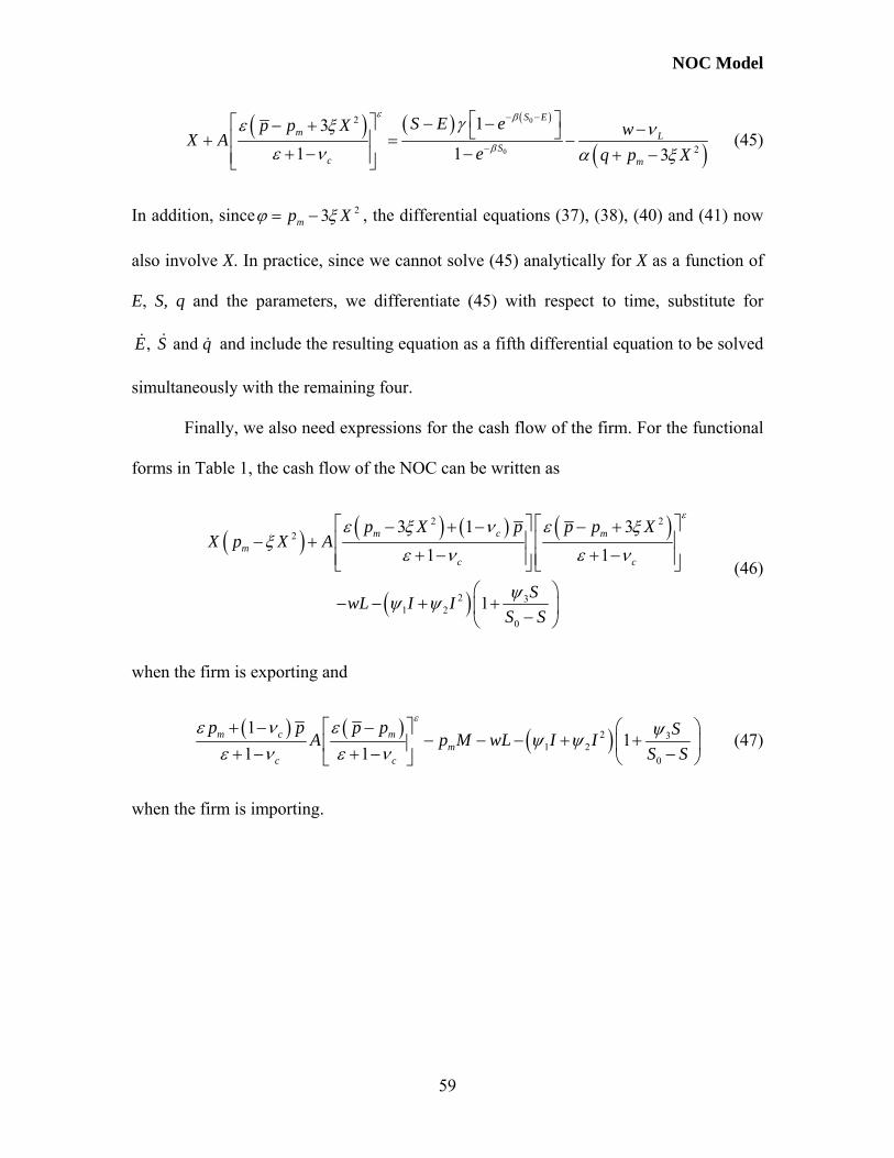
NOC Model
( ) ( ) ( )
( )0
0
2
2
131 1 3
S Em L
Sc m
S E ep p X wX Ae q p X
ε β
β
γε ξ νε ν α ξ
− −
−
⎡ ⎤⎡ ⎤ − −− + −⎣ ⎦⎢ ⎥+ = −+ − − + −⎢ ⎥⎣ ⎦
(45)
In addition, since 23mp Xϕ ξ= − , the differential equations (37), (38), (40) and (41) now
also involve X. In practice, since we cannot solve (45) analytically for X as a function of
E, S, q and the parameters, we differentiate (45) with respect to time, substitute for
, and E S&& &q and include the resulting equation as a fifth differential equation to be solved
simultaneously with the remaining four.
Finally, we also need expressions for the cash flow of the firm. For the functional
forms in Table 1, the cash flow of the NOC can be written as
( ) ( ) ( ) ( )
( )
2 22
2 31 2
0
3 1 31 1
1
m c mm
c
p X p p p XX p X A
SwL I IS S
c
εε ξ ν ε ξ
ξε ν ε ν
ψψ ψ
⎡ ⎤ ⎡− + − − +⎢ ⎥ ⎢− +
+ − + −⎢ ⎥ ⎢⎣ ⎦ ⎣⎛ ⎞
− − + +⎜ ⎟−⎝ ⎠
⎤⎥⎥⎦ (46)
when the firm is exporting and
( ) ( ) ( )2 31 2
0
11
1 1m c m
mc c
p p p p SA p M wL I IS S
εε ν ε ψψ ψ
ε ν ε ν+ − −⎡ ⎤ ⎛ ⎞
− − − + +⎜⎢ ⎥+ − + − −⎝ ⎠⎣ ⎦⎟ (47)
when the firm is importing.
59


