2Object-Based and Image-Based ImageRepresentations
The representation of spatial objects and their environment is an important issue in appli-
cations of computer graphics, game programming, computer vision, image processing,
robotics, pattern recognition, and computational geometry (e.g., [91, 1636, 1637, 1811]).
The problem also arises in building databases to support them (e.g., [1638]). We assume
that the objects are connected1 although their environment need not be. The objects and
their environment are usually decomposed into collections of more primitive elements
(termed cells) each of which has a location in space, a size, and a shape. These ele-
ments can either be subobjects of varying shape (e.g., a table consists of a flat top in
the form of a rectangle and four legs in the form of rods whose lengths dominate their
cross-sectional areas), or they can have a uniform shape. The former yields an object-
based decomposition; the latter yields an image-based, or cell-based, decomposition.
Another way of characterizing these two decompositions is that the former decomposes
the objects, while the latter decomposes the environment in which the objects lie. This
distinction is used commonly in computer graphics to characterize algorithms as being
either object-space or image-space, respectively [622].
Each of the decompositions has its advantages and disadvantages. They depend
primarily on the nature of the queries that are posed to the database. The most general
queries ask where, what, who, why, and how. The ones that are relevant to our application
are where and what [1642]. They are stated more formally as follows:
1. Feature query: Given an object, determine its constituent cells (i.e., their locations
in space).
2. Location query: Given a cell (i.e., a location in space), determine the identity of the
object (or objects) of which it is a member, as well as the remaining constituent cells
of the object (or objects).
Not surprisingly, the queries can be classified using the same terminology that we
used in the characterization of the decomposition. In particular, we can either try to find
the cells (i.e., their locations in space) occupied by an object or find the objects that
overlap a cell (i.e., a location in space). If objects are associated with cells so that a cell
contains the identity of the relevant object (or objects), then the feature query is analogous
to retrieval by contents while the location query is analogous to retrieval by location. As
we will see, it is important to note that there is a distinction between a location in space
and the address where information about the location is stored, which, unfortunately, is
often erroneously assumed to be the same.
1 Intuitively, this means that a d-dimensional object cannot be decomposed into disjoint subobjects
so that the subobjects are not adjacent in a (d − 1)-dimensional sense.
191
Chapter 2
Object-Based and Image-Based
Image Representations
A
C
B
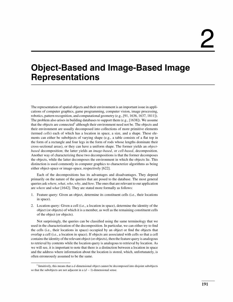
Figure 2.1
Example collection of three objects
and the cells that they occupy.
The feature and location queries are the basis of two more general classes of queries.
In particular, the feature query is a member of a broader class of queries described
collectively as being feature-based (also object-based), and the location query is a
member of a broader class of queries described collectively as being location-based (also
image-based or cell-based). In computational geometry, the location query is known as
the point location query or problem (e.g., [1511, 196] and Sections 2.1.3.2 and 2.1.3.3).
In other domains, it is also commonly referred to as a point query, in which case we
must be careful to distinguish it from its narrower and broader definitions. In particular,
in database applications, a point query has a narrower definition—it is really an exact
match query as it seeks to determine if the data point corresponding to the location is in the
database (e.g., [1046] and the introduction to Chapter 1), and thus whenever possible we
use the term exact match query in this context. On the other hand, in computer graphics
applications, the point query has a broader definition and is often synonymous with the
related “pick” operation (e.g., [622]), which is used to find an object that contains a
given location l, and if there is none, then to find the nearest object to l. In order to
avoid overloading the term point query in this chapter we use the term nearest object
query when a satisfactory response includes the nearest object should no object exist
that contains l.2 Therefore, in this chapter, the term point query has the same meaning
as in Chapter 3, where the response is restricted to the objects that contain l. The class
of location-based queries includes the numerous variants of the window query, which
retrieves the objects that cover an arbitrary region (often rectangular). All of these queries
are used in several applications including geographic information systems (e.g., [72,
1645]) and spatial data mining (e.g., [1953]).
The most common representation of the objects and their environment is as a col-
lection of cells of uniform size and shape (termed pixels and voxels in two and three
dimensions, respectively) all of whose boundaries (with dimensionality one less than
that of the cells) are of unit size. Since the cells are uniform, there exists a way of re-
ferring to their locations in space relative to a fixed reference point (e.g., the origin of
the coordinate system). An example of a location of a cell in space is a set of coordinate
values that enables us to find it in the d-dimensional space of the environment in which
it lies. Once again, we reiterate that it should be clear that the concept of the location of
a cell in space is quite different from that of the address of a cell, which is the physical
location (e.g., in memory, on disk), if any, where some of the information associated
with the cell is stored. This distinction between the location in space of a cell and the
address of a cell is important, and we shall make use of it often.
In most applications (including most of the ones that we consider here), the bound-
aries (i.e., edges and faces in two and three dimensions, respectively) of the cells are
parallel to the coordinate axes. In our discussion, we assume that the cells making up a
particular object are contiguous (i.e., adjacent) and that a different, unique value is asso-
ciated with each distinct object, thereby enabling us to distinguish between the objects.
Depending on the underlying representation, this value may be stored with the cells. For
example, Figure 2.1 contains three two-dimensional objects, A, B, and C, and their corre-
sponding cells. Note that, although it is not the case in this example, objects are allowed
to overlap, which means that a cell may be associated with more than one object. Here
we assume, without loss of generality, that the volume of the overlap must be an integer
multiple of the volume of a cell (i.e., pixels, voxels, etc.).
The shape of an object o can be represented either by the interiors of the cells making
up o, or by the subset of the boundaries of those cells making up o that are adjacent to the
boundary of o. In particular, interior-based methods represent an object o by using the
locations in space of the cells that make up o, while boundary-based methods represent
o by using the locations in space of the cells that are adjacent to the boundary of o.
2 A more general term is nearest neighbor query, which is discussed in a more general context and
in much greater detail in Sections 4.1–4.3 of Chapter 4.
192
Section 2.1
Interior-Based Representations
In general, interior-based representations make it very easy to calculate properties of
an object such as its mass and, depending on the nature of the aggregation process, to
determine the value associated with any point (i.e., location) in the space covered by a
cell in the object. On the other hand, boundary-based representations make it easy to
obtain the boundary of an object.
Regardless of the representation that is used, the generation of responses to the
feature and location queries is facilitated by building an index (i.e., the result of a sort)
either on the objects or on their locations in space, and implementing it using an access
structure that correlates the objects with the locations. Ideally, we want to be able to
answer both types of queries with one representation. This is somewhat tricky, but, as
we will show, it is doable.
The rest of this chapter is organized as follows. Section 2.1 discusses interior-based
representations. These are the most prevalent, and thus this discussion forms the main
part of the chapter. Section 2.2 discusses boundary-based representations. The discus-
sion in these sections shows how some of the representations can be made more compact
by aggregating similar elements. These elements are usually identically valued contigu-
ous cells (possibly adjacent to identically oriented boundary elements) or even objects
that, ideally, are in proximity. The representations can be made even more compact by
recording only the differences between the elements. The use of difference-based com-
paction methods is the subject of Section 2.3. Many of the representations that we have
described are based on the principle of recursive decomposition of the underlying space
(as well as the aggregation of the results of the decomposition). Therefore, we conclude
in Section 2.4 with a brief historical overview of this principle and some of its early uses.
As stated earlier, most of our discussion assumes that the objects can be decomposed
into cells whose boundaries are parallel to the coordinate axes. Nevertheless, we discuss
the representation of objects with boundaries that are hyperplanes (i.e., straight lines
and planar faces for two- and three-dimensional objects, respectively), as well as objects
with arbitrary boundaries (e.g., edges of arbitrary slope, nonplanar faces). In this case,
the representation of the underlying environment is usually, but not always, based on a
decomposition into cells whose boundaries are parallel to the coordinate axes.
2.1 Interior-Based Representations
In this section, we focus on interior-based representations. Section 2.1.1 examines
representations based on collections of unit-size cells. An alternative class of interior-
based representations of the objects and their environment removes the stipulation that
the cells that make up the object collection be a unit size and permits their sizes to
vary. The varying-sized cells are termed blocks and are the subject of Section 2.1.2. The
representations described in Sections 2.1.1 and 2.1.2 assume that each unit-size cell or
block is contained entirely in one or more objects. A cell or block cannot be partially
contained in two objects. This means that either each cell in a block belongs to the same
object or objects, or that all of the cells in the block do not belong to any of the objects.
Section 2.1.3 permits both the blocks and the objects to be arbitrary polyhedra while
not allowing them to intersect, although permitting them to have common boundaries.
Section 2.1.4 permits a cell or block to be a part of more than one object and does not
require the cell or block to be contained in its entirety in these objects. In other words,
a cell or a block may overlap several objects without being completely contained in
them. This also has the effect of permitting the representation of collections of objects
whose boundaries do not coincide with the boundaries of the underlying blocks and also
permitting them to intersect (i.e., overlap). Section 2.1.5 examines the use of hierarchies
of space and objects that enable efficient responses to both the feature and location
queries.
193
Section 2.1
Interior-Based Representations
(a) (b)
(c) (d)
(e) (f)
(g) (h)
(i)
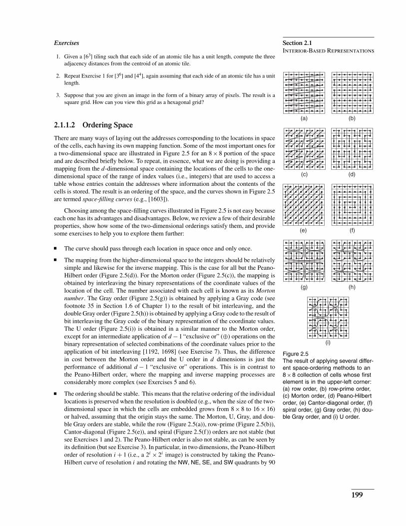
Figure 2.5
The result of applying several differ-
ent space-ordering methods to an
8 × 8 collection of cells whose first
element is in the upper-left corner:
(a) row order, (b) row-prime order,
(c) Morton order, (d) Peano-Hilbert
order, (e) Cantor-diagonal order, (f)
spiral order, (g) Gray order, (h) dou-
ble Gray order, and (i) U order.
Exercises
1. Given a [63] tiling such that each side of an atomic tile has a unit length, compute the three
adjacency distances from the centroid of an atomic tile.
2. Repeat Exercise 1 for [36] and [44], again assuming that each side of an atomic tile has a unit
length.
3. Suppose that you are given an image in the form of a binary array of pixels. The result is a
square grid. How can you view this grid as a hexagonal grid?
2.1.1.2 Ordering Space
There are many ways of laying out the addresses corresponding to the locations in space
of the cells, each having its own mapping function. Some of the most important ones for
a two-dimensional space are illustrated in Figure 2.5 for an 8 × 8 portion of the space
and are described briefly below. To repeat, in essence, what we are doing is providing a
mapping from the d-dimensional space containing the locations of the cells to the one-
dimensional space of the range of index values (i.e., integers) that are used to access a
table whose entries contain the addresses where information about the contents of the
cells is stored. The result is an ordering of the space, and the curves shown in Figure 2.5
are termed space-filling curves (e.g., [1603]).
Choosing among the space-filling curves illustrated in Figure 2.5 is not easy because
each one has its advantages and disadvantages. Below, we review a few of their desirable
properties, show how some of the two-dimensional orderings satisfy them, and provide
some exercises to help you to explore them further:
The curve should pass through each location in space once and only once.
The mapping from the higher-dimensional space to the integers should be relatively
simple and likewise for the inverse mapping. This is the case for all but the Peano-
Hilbert order (Figure 2.5(d)). For the Morton order (Figure 2.5(c)), the mapping is
obtained by interleaving the binary representations of the coordinate values of the
location of the cell. The number associated with each cell is known as its Morton
number. The Gray order (Figure 2.5(g)) is obtained by applying a Gray code (see
footnote 35 in Section 1.6 of Chapter 1) to the result of bit interleaving, and the
double Gray order (Figure 2.5(h)) is obtained by applying a Gray code to the result of
bit interleaving the Gray code of the binary representation of the coordinate values.
The U order (Figure 2.5(i)) is obtained in a similar manner to the Morton order,
except for an intermediate application of d − 1 “exclusive or” (⊕) operations on the
binary representation of selected combinations of the coordinate values prior to the
application of bit interleaving [1192, 1698] (see Exercise 7). Thus, the difference
in cost between the Morton order and the U order in d dimensions is just the
performance of additional d − 1 “exclusive or” operations. This is in contrast to
the Peano-Hilbert order, where the mapping and inverse mapping processes are
considerably more complex (see Exercises 5 and 6).
The ordering should be stable. This means that the relative ordering of the individual
locations is preserved when the resolution is doubled (e.g., when the size of the two-
dimensional space in which the cells are embedded grows from 8 × 8 to 16 × 16)
or halved, assuming that the origin stays the same. The Morton, U, Gray, and dou-
ble Gray orders are stable, while the row (Figure 2.5(a)), row-prime (Figure 2.5(b)),
Cantor-diagonal (Figure 2.5(e)), and spiral (Figure 2.5(f )) orders are not stable (but
see Exercises 1 and 2). The Peano-Hilbert order is also not stable, as can be seen by
its definition (but see Exercise 3). In particular, in two dimensions, the Peano-Hilbert
order of resolution i + 1 (i.e., a 2i × 2i image) is constructed by taking the Peano-
Hilbert curve of resolution i and rotating the NW, NE, SE, and SW quadrants by 90
199
Chapter 2
Object-Based and Image-Based
Image Representations
A1
C1
B1
W4
W1
(a)
W2
B2W3
1
B1W3
6
B2
C1
2 6
W4
5
W1A1
4 5
W2
y: y:
y:
x:
x:
(b)
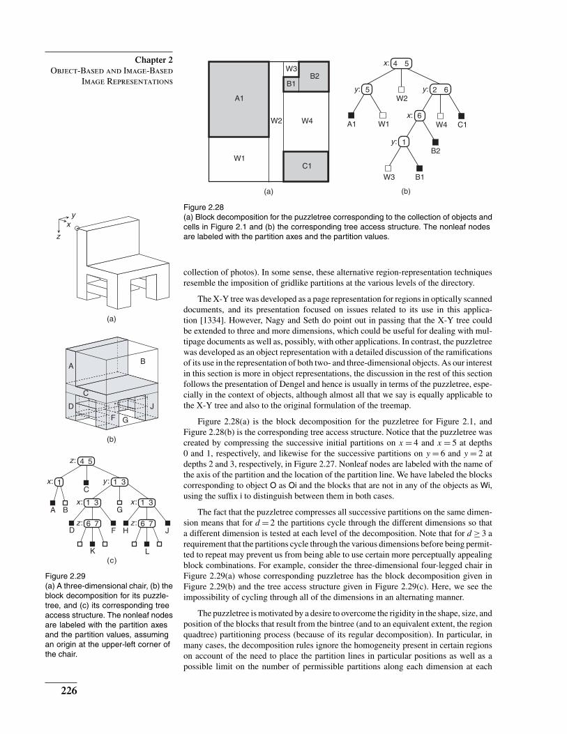
Figure 2.28
(a) Block decomposition for the puzzletree corresponding to the collection of objects and
cells in Figure 2.1 and (b) the corresponding tree access structure. The nonleaf nodes
are labeled with the partition axes and the partition values.
C
G
G
(b)
(c)
xy
z
1
BA
4 5
x:
z:
1 3y :
D F
1 3x :
H J
1 3x :
6 7
K
z : 6 7z :
L
D
F
J
BA
C
(a)
Figure 2.29
(a) A three-dimensional chair, (b) the
block decomposition for its puzzle-
tree, and (c) its corresponding tree
access structure. The nonleaf nodes
are labeled with the partition axes
and the partition values, assuming
an origin at the upper-left corner of
the chair.
collection of photos). In some sense, these alternative region-representation techniques
resemble the imposition of gridlike partitions at the various levels of the directory.
The X-Y tree was developed as a page representation for regions in optically scanned
documents, and its presentation focused on issues related to its use in this applica-
tion [1334]. However, Nagy and Seth do point out in passing that the X-Y tree could
be extended to three and more dimensions, which could be useful for dealing with mul-
tipage documents as well as, possibly, with other applications. In contrast, the puzzletree
was developed as an object representation with a detailed discussion of the ramifications
of its use in the representation of both two- and three-dimensional objects. As our interest
in this section is more in object representations, the discussion in the rest of this section
follows the presentation of Dengel and hence is usually in terms of the puzzletree, espe-
cially in the context of objects, although almost all that we say is equally applicable to
the X-Y tree and also to the original formulation of the treemap.
Figure 2.28(a) is the block decomposition for the puzzletree for Figure 2.1, and
Figure 2.28(b) is the corresponding tree access structure. Notice that the puzzletree was
created by compressing the successive initial partitions on x = 4 and x = 5 at depths
0 and 1, respectively, and likewise for the successive partitions on y = 6 and y = 2 at
depths 2 and 3, respectively, in Figure 2.27. Nonleaf nodes are labeled with the name of
the axis of the partition and the location of the partition line. We have labeled the blocks
corresponding to object O as Oi and the blocks that are not in any of the objects as Wi,
using the suffix i to distinguish between them in both cases.
The fact that the puzzletree compresses all successive partitions on the same dimen-
sion means that for d = 2 the partitions cycle through the different dimensions so that
a different dimension is tested at each level of the decomposition. Note that for d ≥ 3 a
requirement that the partitions cycle through the various dimensions before being permit-
ted to repeat may prevent us from being able to use certain more perceptually appealing
block combinations. For example, consider the three-dimensional four-legged chair in
Figure 2.29(a) whose corresponding puzzletree has the block decomposition given in
Figure 2.29(b) and the tree access structure given in Figure 2.29(c). Here, we see the
impossibility of cycling through all of the dimensions in an alternating manner.
The puzzletree is motivated by a desire to overcome the rigidity in the shape, size, and
position of the blocks that result from the bintree (and to an equivalent extent, the region
quadtree) partitioning process (because of its regular decomposition). In particular, in
many cases, the decomposition rules ignore the homogeneity present in certain regions
on account of the need to place the partition lines in particular positions as well as a
possible limit on the number of permissible partitions along each dimension at each
226
Section 2.1
Interior-Based Representations
CD
AB
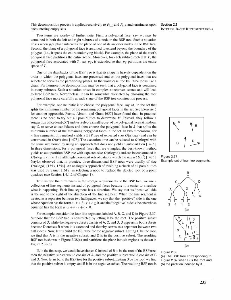
Figure 2.37
Example set of four line segments.
B
C D
A D
3 4 1 2
5 6
C
D
AB
1
2
3
45
6
(a)
(b)
Figure 2.38
(a) The BSP tree corresponding to
Figure 2.37 when B is the root and
(b) the partition induced by it.
This decomposition process is applied recursively to Pk,L and Pk,R and terminates upon
encountering empty sets.
Two items are worthy of further note. First, a polygonal face, say pi, may be
contained in both the left and right subtrees of a node in the BSP tree. Such a situation
arises when pi’s plane intersects the plane of one of its ancestor nodes in the BSP tree.
Second, the plane of a polygonal face is assumed to extend beyond the boundary of the
polygon (i.e., it spans the entire underlying block). For example, the plane of the root’s
polygonal face partitions the entire scene. Moreover, for each subtree rooted at T , the
polygonal face associated with T , say pT , is extended so that pT partitions the entire
space of T .
One of the drawbacks of the BSP tree is that its shape is heavily dependent on the
order in which the polygonal faces are processed and on the polygonal faces that are
selected to serve as the partitioning planes. In the worst case, the BSP tree looks like a
chain. Furthermore, the decomposition may be such that a polygonal face is contained
in many subtrees. Such a situation arises in complex nonconvex scenes and will lead
to large BSP trees. Nevertheless, it can be somewhat alleviated by choosing the root
polygonal face more carefully at each stage of the BSP tree construction process.
For example, one heuristic is to choose the polygonal face, say M , in the set that
splits the minimum number of the remaining polygonal faces in the set (see Exercise 5
for another approach). Fuchs, Abram, and Grant [657] have found that, in practice,
there is no need to try out all possibilities to determine M . Instead, they follow a
suggestion of Kedem [657] and just select a small subset of the polygonal faces at random,
say S, to serve as candidates and then choose the polygonal face in S that splits the
minimum number of the remaining polygonal faces in the set. In two dimensions, for
n line segments, this method yields a BSP tree of expected size O(nlogn) and can be
constructed in O(n2) time [1475]. The execution time can be reduced to O(nlogn) with
the same size bound by using an approach that does not yield an autopartition [1475].
In three dimensions, for n polygonal faces that are triangles, the best-known method
yields an autopartition BSP tree with expected size O(nlog2n) and can be constructed in
O(nlog3n) time [18], although there exist sets of data for which the size is �(n2) [1475].
Naylor observed that, in practice, three-dimensional BSP trees were usually of size
O(nlogn) [1353, 1354]. An analogous approach of avoiding a check of all possibilities
was used by Samet [1618] in selecting a node to replace the deleted root of a point
quadtree (see Section 1.4.1.2 of Chapter 1).
To illustrate the differences in the storage requirements of the BSP tree, we use a
collection of line segments instead of polygonal faces because it is easier to visualize
what is happening. Each line segment has a direction. We say that its “positive” side
is the one to the right of the direction of the line segment. When the line segment is
treated as a separator between two halfspaces, we say that the “positive” side is the one
whose equation has the form a . x +b . y + c ≥ 0, and the “negative” side is the one whose
equation has the form a . x + b . y + c < 0.
For example, consider the four line segments labeled A, B, C, and D in Figure 2.37.
Suppose that the BSP tree is constructed by letting B be the root. The positive subset
consists of D, while the negative subset consists of A, C, and D. D appears in both subsets
because D crosses B when it is extended and thereby serves as a separator between two
halfspaces. Now, let us build the BSP tree for the negative subset. Letting C be the root,
we find that A is in the negative subset, and D is in the positive subset. The resulting
BSP tree is shown in Figure 2.38(a) and partitions the plane into six regions as shown in
Figure 2.38(b).
If, in the first step, we would have chosen C instead of B to be the root of the BSP tree,
then the negative subset would consist of A, and the positive subset would consist of B
and D. Now, let us build the BSP tree for the positive subset. Letting D be the root, we find
that the positive subset is empty, and B is in the negative subset. The resulting BSP tree is
235
Section 2.1
Interior-Based Representations
(a) (b)
(c) (d)
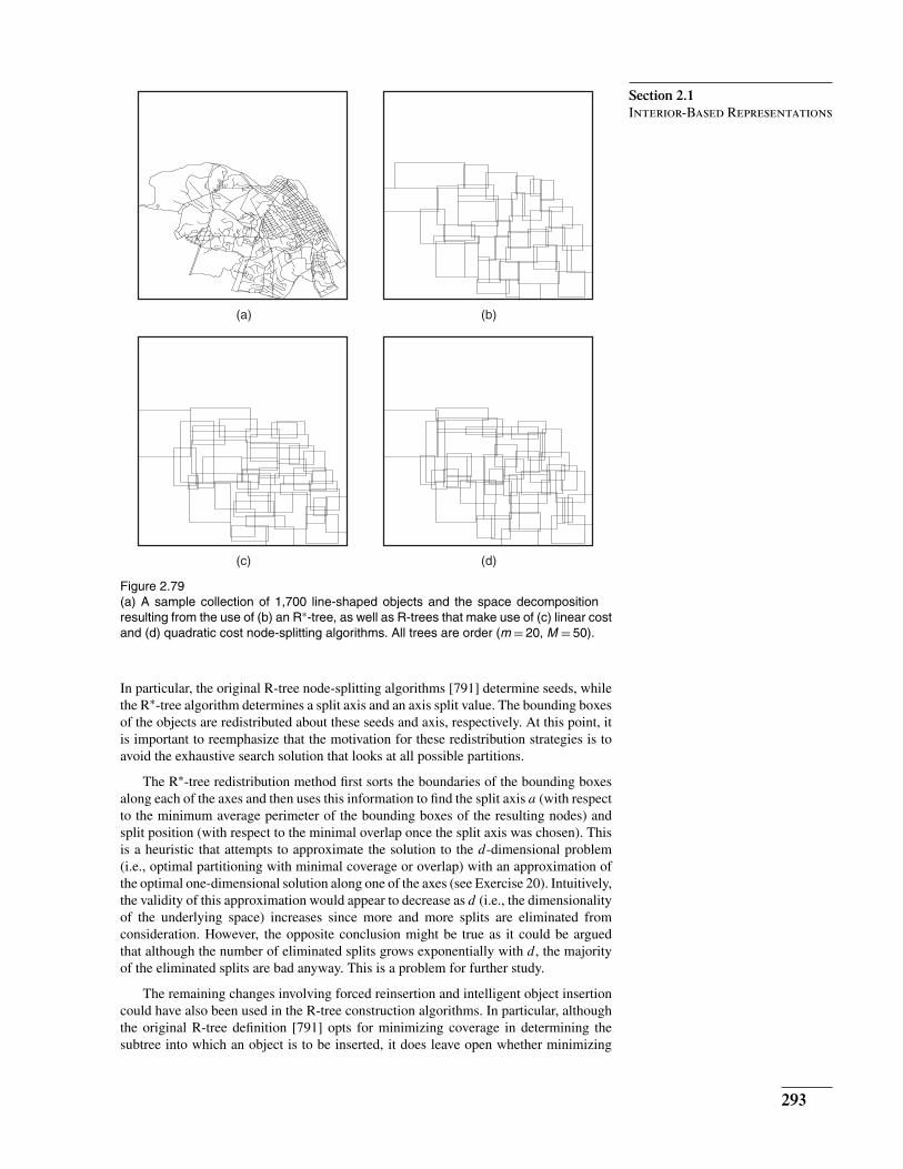
Figure 2.79
(a) A sample collection of 1,700 line-shaped objects and the space decomposition
resulting from the use of (b) an R∗-tree, as well as R-trees that make use of (c) linear cost
and (d) quadratic cost node-splitting algorithms. All trees are order (m = 20, M = 50).
In particular, the original R-tree node-splitting algorithms [791] determine seeds, while
the R∗-tree algorithm determines a split axis and an axis split value. The bounding boxes
of the objects are redistributed about these seeds and axis, respectively. At this point, it
is important to reemphasize that the motivation for these redistribution strategies is to
avoid the exhaustive search solution that looks at all possible partitions.
The R∗-tree redistribution method first sorts the boundaries of the bounding boxes
along each of the axes and then uses this information to find the split axis a (with respect
to the minimum average perimeter of the bounding boxes of the resulting nodes) and
split position (with respect to the minimal overlap once the split axis was chosen). This
is a heuristic that attempts to approximate the solution to the d-dimensional problem
(i.e., optimal partitioning with minimal coverage or overlap) with an approximation of
the optimal one-dimensional solution along one of the axes (see Exercise 20). Intuitively,
the validity of this approximation would appear to decrease as d (i.e., the dimensionality
of the underlying space) increases since more and more splits are eliminated from
consideration. However, the opposite conclusion might be true as it could be argued
that although the number of eliminated splits grows exponentially with d, the majority
of the eliminated splits are bad anyway. This is a problem for further study.
The remaining changes involving forced reinsertion and intelligent object insertion
could have also been used in the R-tree construction algorithms. In particular, although
the original R-tree definition [791] opts for minimizing coverage in determining the
subtree into which an object is to be inserted, it does leave open whether minimizing
293
Chapter 2
Object-Based and Image-Based
Image Representations
ENCW(e)CF(FCW(e))CCV(VEND(e))
EPCW(e)CCF(FCW(e))CV(VSTART(e))FCW(e)
e
(a)
VEND(e) VSTART(e)
FCCW(e)EPCCW(e)CCF(FCCW(e))CV(VEND(e))
ENCCW(e)CF(FCCW(e))CCV(VSTART(e))
EPCCW(e)CV(VEND(e))
CCF(FCCW(e))
CF(FCCW(e))CCV(VSTART(e))
ENCCW(e)
VSTART(e)
VEND(e)
CCF(FCW
(e))
CV(VSTART(e
))
EPCW(e
)
ENCW(e
)
CCV(VEND(e
))
CF(FCW
(e))
eFCW(e)
FCCW(e)
(b)
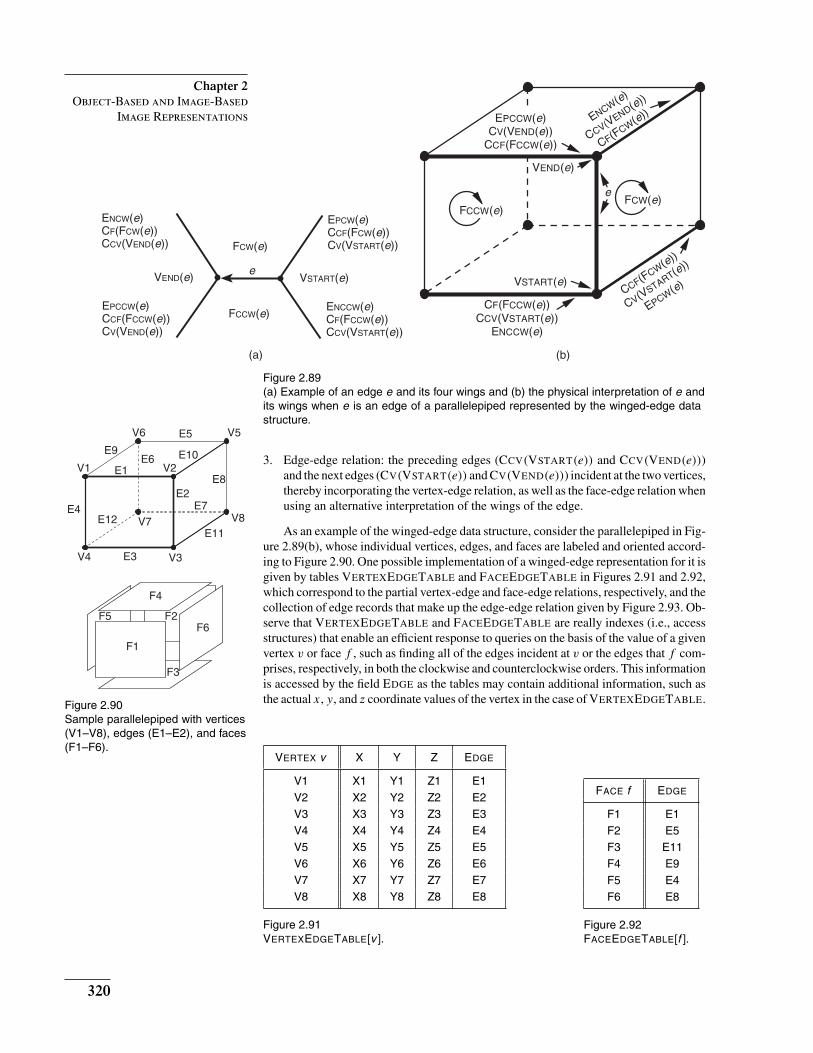
Figure 2.89
(a) Example of an edge e and its four wings and (b) the physical interpretation of e and
its wings when e is an edge of a parallelepiped represented by the winged-edge data
structure.
E9
E5V6 V5
E10V2E1
E6
V7
E2E7
E8
V8
V3E3
E12E4
V1
V4
E11
F1
F2
F3
F4
F5F6
Figure 2.90
Sample parallelepiped with vertices
(V1–V8), edges (E1–E2), and faces
(F1–F6).
3. Edge-edge relation: the preceding edges (CCV(VSTART(e)) and CCV(VEND(e)))
and the next edges (CV(VSTART(e)) and CV(VEND(e))) incident at the two vertices,
thereby incorporating the vertex-edge relation, as well as the face-edge relation when
using an alternative interpretation of the wings of the edge.
As an example of the winged-edge data structure, consider the parallelepiped in Fig-
ure 2.89(b), whose individual vertices, edges, and faces are labeled and oriented accord-
ing to Figure 2.90. One possible implementation of a winged-edge representation for it is
given by tables VERTEXEDGETABLE and FACEEDGETABLE in Figures 2.91 and 2.92,
which correspond to the partial vertex-edge and face-edge relations, respectively, and the
collection of edge records that make up the edge-edge relation given by Figure 2.93. Ob-
serve that VERTEXEDGETABLE and FACEEDGETABLE are really indexes (i.e., access
structures) that enable an efficient response to queries on the basis of the value of a given
vertex v or face f , such as finding all of the edges incident at v or the edges that f com-
prises, respectively, in both the clockwise and counterclockwise orders. This information
is accessed by the field EDGE as the tables may contain additional information, such as
the actual x, y, and z coordinate values of the vertex in the case of VERTEXEDGETABLE.
VERTEX v X Y Z EDGE
V1 X1 Y1 Z1 E1
V2 X2 Y2 Z2 E2
V3 X3 Y3 Z3 E3
V4 X4 Y4 Z4 E4
V5 X5 Y5 Z5 E5
V6 X6 Y6 Z6 E6
V7 X7 Y7 Z7 E7
V8 X8 Y8 Z8 E8
Figure 2.91
VERTEXEDGETABLE[v ].
FACE f EDGE
F1 E1
F2 E5
F3 E11
F4 E9
F5 E4
F6 E8
Figure 2.92
FACEEDGETABLE[f ].
320
Chapter 2
Object-Based and Image-Based
Image Representations
F
E
G
D
(a)
F
E
G
D
(b)
F
E
G
D
(c)
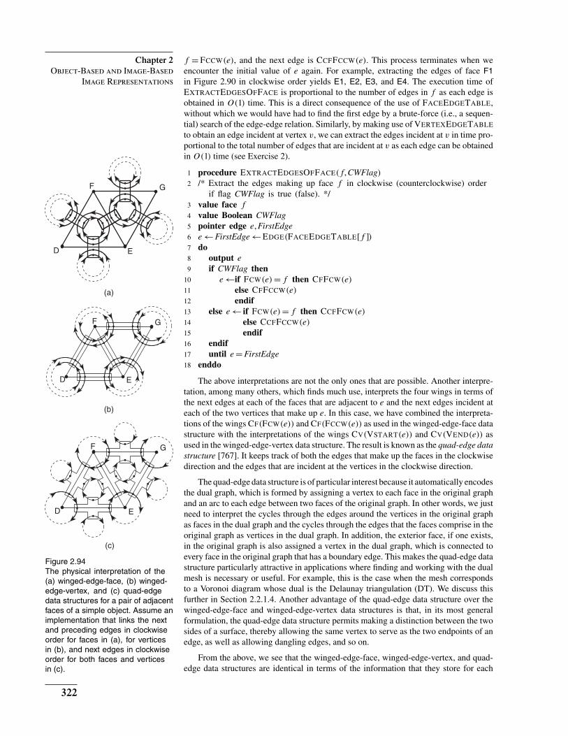
Figure 2.94
The physical interpretation of the
(a) winged-edge-face, (b) winged-
edge-vertex, and (c) quad-edge
data structures for a pair of adjacent
faces of a simple object. Assume an
implementation that links the next
and preceding edges in clockwise
order for faces in (a), for vertices
in (b), and next edges in clockwise
order for both faces and vertices
in (c).
f = FCCW(e), and the next edge is CCFFCCW(e). This process terminates when we
encounter the initial value of e again. For example, extracting the edges of face F1
in Figure 2.90 in clockwise order yields E1, E2, E3, and E4. The execution time of
EXTRACTEDGESOFFACE is proportional to the number of edges in f as each edge is
obtained in O(1) time. This is a direct consequence of the use of FACEEDGETABLE,
without which we would have had to find the first edge by a brute-force (i.e., a sequen-
tial) search of the edge-edge relation. Similarly, by making use of VERTEXEDGETABLE
to obtain an edge incident at vertex v, we can extract the edges incident at v in time pro-
portional to the total number of edges that are incident at v as each edge can be obtained
in O(1) time (see Exercise 2).
1 procedure EXTRACTEDGESOFFACE(f,CWFlag)
2 /* Extract the edges making up face f in clockwise (counterclockwise) order
if flag CWFlag is true (false). */
3 value face f
4 value Boolean CWFlag
5 pointer edge e,FirstEdge
6 e ← FirstEdge ← EDGE(FACEEDGETABLE[f ])
7 do
8 output e
9 if CWFlag then
10 e ←if FCW(e) = f then CFFCW(e)
11 else CFFCCW(e)
12 endif
13 else e ← if FCW(e) = f then CCFFCW(e)
14 else CCFFCCW(e)
15 endif
16 endif
17 until e = FirstEdge
18 enddo
The above interpretations are not the only ones that are possible. Another interpre-
tation, among many others, which finds much use, interprets the four wings in terms of
the next edges at each of the faces that are adjacent to e and the next edges incident at
each of the two vertices that make up e. In this case, we have combined the interpreta-
tions of the wings CF(FCW(e)) and CF(FCCW(e)) as used in the winged-edge-face data
structure with the interpretations of the wings CV(VSTART(e)) and CV(VEND(e)) as
used in the winged-edge-vertex data structure. The result is known as the quad-edge data
structure [767]. It keeps track of both the edges that make up the faces in the clockwise
direction and the edges that are incident at the vertices in the clockwise direction.
The quad-edge data structure is of particular interest because it automatically encodes
the dual graph, which is formed by assigning a vertex to each face in the original graph
and an arc to each edge between two faces of the original graph. In other words, we just
need to interpret the cycles through the edges around the vertices in the original graph
as faces in the dual graph and the cycles through the edges that the faces comprise in the
original graph as vertices in the dual graph. In addition, the exterior face, if one exists,
in the original graph is also assigned a vertex in the dual graph, which is connected to
every face in the original graph that has a boundary edge. This makes the quad-edge data
structure particularly attractive in applications where finding and working with the dual
mesh is necessary or useful. For example, this is the case when the mesh corresponds
to a Voronoi diagram whose dual is the Delaunay triangulation (DT). We discuss this
further in Section 2.2.1.4. Another advantage of the quad-edge data structure over the
winged-edge-face and winged-edge-vertex data structures is that, in its most general
formulation, the quad-edge data structure permits making a distinction between the two
sides of a surface, thereby allowing the same vertex to serve as the two endpoints of an
edge, as well as allowing dangling edges, and so on.
From the above, we see that the winged-edge-face, winged-edge-vertex, and quad-
edge data structures are identical in terms of the information that they store for each
322
Chapter 2
Object-Based and Image-Based
Image Representations
Exercise
1. Show how the half-edge-vertex data structure (i.e., the vertex variant of the half-edge data
structure) is closely related to the counterclockwise variant of the corner lath data structure In
this case, recall from Exercise 11 of Section 2.2.1.2 that, given half-edge L, the vertex variant
of the half-edge data structure is defined in terms of CV(L) and CCV(L).
2.2.1.4 Voronoi Diagrams, Delaunay Graphs, and
Delaunay Triangulations
In Sections 2.2.1.2 and 2.2.1.3, we pointed out that an advantage of the quad-edge
interpretation of the winged-edge data structure over the other interpretations (e.g., the
winged-edge-face and winged-edge-vertex) is that the quad-edge data structure is a self-
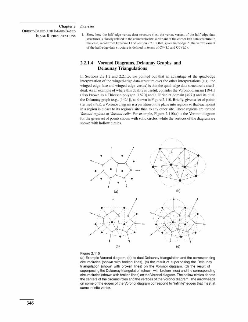
dual. As an example of where this duality is useful, consider the Voronoi diagram [1941]
(also known as a Thiessen polygon [1870] and a Dirichlet domain [497]) and its dual,
the Delaunay graph (e.g., [1424]), as shown in Figure 2.110. Briefly, given a set of points
(termed sites), a Voronoi diagram is a partition of the plane into regions so that each point
in a region is closer to its region’s site than to any other site. These regions are termed
Voronoi regions or Voronoi cells. For example, Figure 2.110(a) is the Voronoi diagram
for the given set of points shown with solid circles, while the vertices of the diagram are
shown with hollow circles.
(a) (b)
(c) (d)
Figure 2.110
(a) Example Voronoi diagram, (b) its dual Delaunay triangulation and the corresponding
circumcircles (shown with broken lines), (c) the result of superposing the Delaunay
triangulation (shown with broken lines) on the Voronoi diagram, (d) the result of
superposing the Delaunay triangulation (shown with broken lines) and the corresponding
circumcircles (shown with broken lines) on the Voronoi diagram. The hollow circles denote
the centers of the circumcircles and the vertices of the Voronoi diagram. The arrowheads
on some of the edges of the Voronoi diagram correspond to “infinite” edges that meet at
some infinite vertex.
346
Chapter 2
Object-Based and Image-Based
Image Representations
(a)
(b)
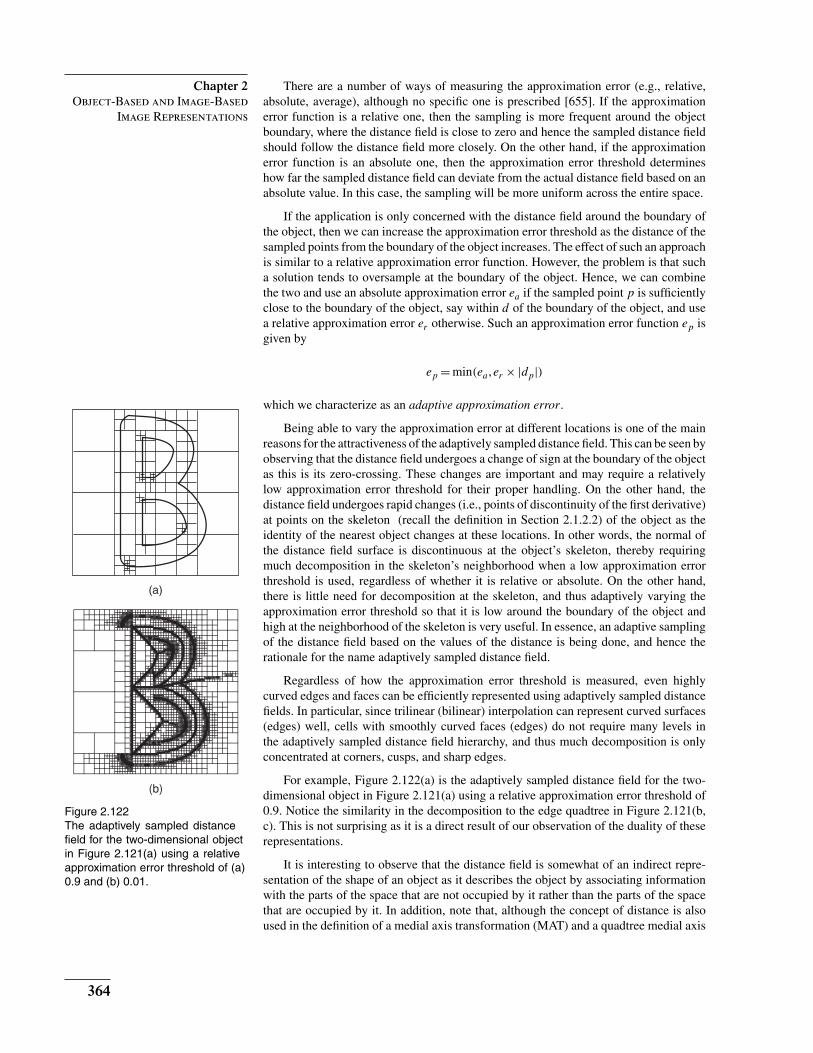
Figure 2.122
The adaptively sampled distance
field for the two-dimensional object
in Figure 2.121(a) using a relative
approximation error threshold of (a)
0.9 and (b) 0.01.
There are a number of ways of measuring the approximation error (e.g., relative,
absolute, average), although no specific one is prescribed [655]. If the approximation
error function is a relative one, then the sampling is more frequent around the object
boundary, where the distance field is close to zero and hence the sampled distance field
should follow the distance field more closely. On the other hand, if the approximation
error function is an absolute one, then the approximation error threshold determines
how far the sampled distance field can deviate from the actual distance field based on an
absolute value. In this case, the sampling will be more uniform across the entire space.
If the application is only concerned with the distance field around the boundary of
the object, then we can increase the approximation error threshold as the distance of the
sampled points from the boundary of the object increases. The effect of such an approach
is similar to a relative approximation error function. However, the problem is that such
a solution tends to oversample at the boundary of the object. Hence, we can combine
the two and use an absolute approximation error ea if the sampled point p is sufficiently
close to the boundary of the object, say within d of the boundary of the object, and use
a relative approximation error er otherwise. Such an approximation error function ep is
given by
ep = min(ea,er × |dp|)
which we characterize as an adaptive approximation error.
Being able to vary the approximation error at different locations is one of the main
reasons for the attractiveness of the adaptively sampled distance field. This can be seen by
observing that the distance field undergoes a change of sign at the boundary of the object
as this is its zero-crossing. These changes are important and may require a relatively
low approximation error threshold for their proper handling. On the other hand, the
distance field undergoes rapid changes (i.e., points of discontinuity of the first derivative)
at points on the skeleton (recall the definition in Section 2.1.2.2) of the object as the
identity of the nearest object changes at these locations. In other words, the normal of
the distance field surface is discontinuous at the object’s skeleton, thereby requiring
much decomposition in the skeleton’s neighborhood when a low approximation error
threshold is used, regardless of whether it is relative or absolute. On the other hand,
there is little need for decomposition at the skeleton, and thus adaptively varying the
approximation error threshold so that it is low around the boundary of the object and
high at the neighborhood of the skeleton is very useful. In essence, an adaptive sampling
of the distance field based on the values of the distance is being done, and hence the
rationale for the name adaptively sampled distance field.
Regardless of how the approximation error threshold is measured, even highly
curved edges and faces can be efficiently represented using adaptively sampled distance
fields. In particular, since trilinear (bilinear) interpolation can represent curved surfaces
(edges) well, cells with smoothly curved faces (edges) do not require many levels in
the adaptively sampled distance field hierarchy, and thus much decomposition is only
concentrated at corners, cusps, and sharp edges.
For example, Figure 2.122(a) is the adaptively sampled distance field for the two-
dimensional object in Figure 2.121(a) using a relative approximation error threshold of
0.9. Notice the similarity in the decomposition to the edge quadtree in Figure 2.121(b,
c). This is not surprising as it is a direct result of our observation of the duality of these
representations.
It is interesting to observe that the distance field is somewhat of an indirect repre-
sentation of the shape of an object as it describes the object by associating information
with the parts of the space that are not occupied by it rather than the parts of the space
that are occupied by it. In addition, note that, although the concept of distance is also
used in the definition of a medial axis transformation (MAT) and a quadtree medial axis
364
Section 2.2
Boundary-Based
Representations
D
A B
C
I
H
G
EF
(a)
D
A B
C
I
H
G
E F
(b)
D
A B
C
I
H
G
EF
(c)
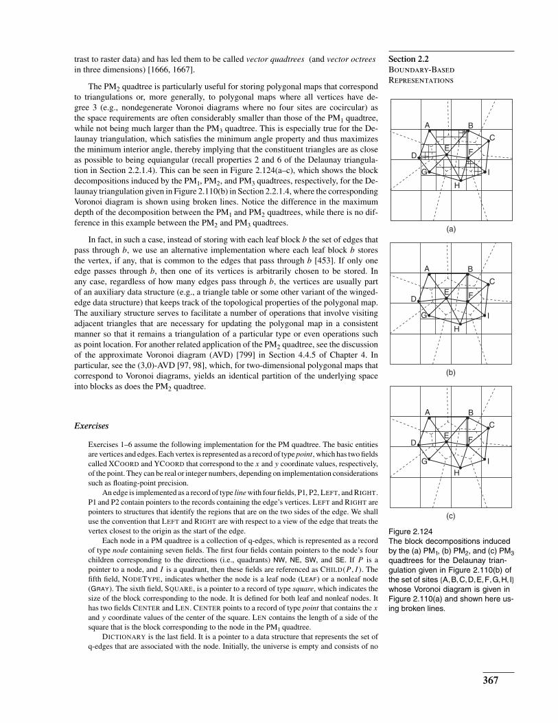
Figure 2.124
The block decompositions induced
by the (a) PM1, (b) PM2, and (c) PM3
quadtrees for the Delaunay trian-
gulation given in Figure 2.110(b) of
the set of sites {A,B,C,D,E,F,G,H,I}
whose Voronoi diagram is given in
Figure 2.110(a) and shown here us-
ing broken lines.
trast to raster data) and has led them to be called vector quadtrees (and vector octrees
in three dimensions) [1666, 1667].
The PM2 quadtree is particularly useful for storing polygonal maps that correspond
to triangulations or, more generally, to polygonal maps where all vertices have de-
gree 3 (e.g., nondegenerate Voronoi diagrams where no four sites are cocircular) as
the space requirements are often considerably smaller than those of the PM1 quadtree,
while not being much larger than the PM3 quadtree. This is especially true for the De-
launay triangulation, which satisfies the minimum angle property and thus maximizes
the minimum interior angle, thereby implying that the constituent triangles are as close
as possible to being equiangular (recall properties 2 and 6 of the Delaunay triangula-
tion in Section 2.2.1.4). This can be seen in Figure 2.124(a–c), which shows the block
decompositions induced by the PM1, PM2, and PM3 quadtrees, respectively, for the De-
launay triangulation given in Figure 2.110(b) in Section 2.2.1.4, where the corresponding
Voronoi diagram is shown using broken lines. Notice the difference in the maximum
depth of the decomposition between the PM1 and PM2 quadtrees, while there is no dif-
ference in this example between the PM2 and PM3 quadtrees.
In fact, in such a case, instead of storing with each leaf block b the set of edges that
pass through b, we use an alternative implementation where each leaf block b stores
the vertex, if any, that is common to the edges that pass through b [453]. If only one
edge passes through b, then one of its vertices is arbitrarily chosen to be stored. In
any case, regardless of how many edges pass through b, the vertices are usually part
of an auxiliary data structure (e.g., a triangle table or some other variant of the winged-
edge data structure) that keeps track of the topological properties of the polygonal map.
The auxiliary structure serves to facilitate a number of operations that involve visiting
adjacent triangles that are necessary for updating the polygonal map in a consistent
manner so that it remains a triangulation of a particular type or even operations such
as point location. For another related application of the PM2 quadtree, see the discussion
of the approximate Voronoi diagram (AVD) [799] in Section 4.4.5 of Chapter 4. In
particular, see the (3,0)-AVD [97, 98], which, for two-dimensional polygonal maps that
correspond to Voronoi diagrams, yields an identical partition of the underlying space
into blocks as does the PM2 quadtree.
Exercises
Exercises 1–6 assume the following implementation for the PM quadtree. The basic entities
are vertices and edges. Each vertex is represented as a record of type point, which has two fields
called XCOORD and YCOORD that correspond to the x and y coordinate values, respectively,
of the point. They can be real or integer numbers, depending on implementation considerations
such as floating-point precision.
An edge is implemented as a record of type line with four fields, P1, P2, LEFT, and RIGHT.
P1 and P2 contain pointers to the records containing the edge’s vertices. LEFT and RIGHT are
pointers to structures that identify the regions that are on the two sides of the edge. We shall
use the convention that LEFT and RIGHT are with respect to a view of the edge that treats the
vertex closest to the origin as the start of the edge.
Each node in a PM quadtree is a collection of q-edges, which is represented as a record
of type node containing seven fields. The first four fields contain pointers to the node’s four
children corresponding to the directions (i.e., quadrants) NW, NE, SW, and SE. If P is a
pointer to a node, and I is a quadrant, then these fields are referenced as CHILD(P,I ). The
fifth field, NODETYPE, indicates whether the node is a leaf node (LEAF) or a nonleaf node
(GRAY). The sixth field, SQUARE, is a pointer to a record of type square, which indicates the
size of the block corresponding to the node. It is defined for both leaf and nonleaf nodes. It
has two fields CENTER and LEN. CENTER points to a record of type point that contains the x
and y coordinate values of the center of the square. LEN contains the length of a side of the
square that is the block corresponding to the node in the PM1 quadtree.
DICTIONARY is the last field. It is a pointer to a data structure that represents the set of
q-edges that are associated with the node. Initially, the universe is empty and consists of no
367

Section 2.2
Boundary-Based
Representations
C
C
D
D
B
B
A
A(a)
C
C
D
D
B
B
A
A(b)
Figure 2.154
Example illustrating the ambiguity
that results when each rectangle is
split into two triangles by adding a
diagonal edge between (a) vertices
B and C and (b) vertices A and D.
(a)
(c) (d)
(b)
Figure 2.155
(a) Restricted quadtree correspond-
ing to the rectangular decomposition
in Figure 2.152(b) and the result
of triangulating it using a (b) two-
triangle rule, (c) four-triangle rule,
and (d) eight-triangle rule.
The newly added points that do not lie on existing edges represent new samples. Thus,
we must also obtain an elevation value for them. There are two choices for some of them
since they fall at the midpoints of edges between the midpoints of both a horizontal and a
vertical edge. We choose to take the average of the two interpolated values. For example,
v is obtained by taking the average of the values obtained by applying linear interpolation
to the elevation values at L and t and the elevation values at u and r. The same technique
is applied to obtain the elevation value at z once we have obtained the elevation values
at x, y, and w.
At this point, let us briefly compare the two different quaternary hierarchical decom-
positions. As we saw, both methods suffer from the alignment problem when we try to
fit a surface through their vertices. However, as we have demonstrated, this problem can
be overcome through the addition of the appropriate triangles and rectangles. For the
triangular decomposition, we obtained a planar surface because we were able to use a
planar triangulation. For the rectangular decomposition, we obtained a nonplanar surface
because it is impossible to fit a plane through the four vertices of each rectangle.
It could be argued that a nonplanar surface is a better approximation of a nonplanar
surface than a planar one, thereby making the rectangular decomposition more attractive
than the triangular decomposition. Of course, we could also fit a nonplanar surface
through the vertices of the triangles. However, it is well-known that the more sample
points that are used in a surface patch, the better is the approximation of the underlying
surface. Thus, such reasoning implies that the rectangular decomposition is preferable
to the triangular decomposition.
An argument could also be made that the planar approximation of the surface
provided by the triangle is preferable to the nonplanar approximation provided by the
rectangle. This is especially true if ease of interpolation is an issue. In fact, we could
also obtain a planar approximation using rectangles by splitting each rectangle into two
triangles by adding a diagonal edge between two opposing vertices. There are two choices
as shown in Figure 2.154. As long as the four vertices are not coplanar, one will result
in a ridgelike planar surface (Figure 2.154(a)), while the other will result in a valleylike
planar surface (Figure 2.154(b)). We usually choose the diagonal edge whose angle is
the most obtuse.
Neither of the above solutions to the alignment problem that employ a quaternary
hierarchical decomposition (whether they use a triangular or rectangular decomposition)
yields a conforming mesh because not all of the polygons that make up the mesh have the
same number of vertices and edges. Nevertheless, the quaternary hierarchical decompo-
sition that makes use of a rectangular quadtree can form the basis of a conforming mesh
and overcome the alignment problem. The idea is to apply a planar triangulation to the
result of transforming the underlying rectangular quadtree to a restricted quadtree [1453,
1771, 1772, 1940]. The restricted quadtree has the property that all rectangles that are
edge neighbors are either of equal size or of ratio 2:1. Such a quadtree is also termed a 1-
irregular quadtree [124], a balanced quadtree [204], and a 1-balanced quadtree [1312].
A somewhat tighter restriction requires that all vertex neighbors either be of equal size or
of ratio 2:1 (termed a 0-balanced quadtree [1312]). It should be clear that a 0-balanced
quadtree is also a 1-balanced quadtree but not vice versa (see Exercise 4).
Given an arbitrary quadtree decomposition, the restricted quadtree is formed by
repeatedly subdividing the larger nodes until the 2:1 ratio holds. For example, Fig-
ure 2.155(a) is the restricted quadtree corresponding to the rectangular decomposition
in Figure 2.152(b). Note that the SE quadrant of Figure 2.152(b) has to be decomposed
once, in contrast to twice when building the hierarchy of rectangles in Figure 2.153(b).
This method of subdivision is also used in finite-element analysis (e.g., [1147]) as part
of a technique called h-refinement [1013] to refine adaptively a mesh that has already
been analyzed, as well as to achieve element compatibility.
405


