MLSP2012 Tutorial:
Manifold Learning: Modeling and
Algorithms
Dr. Raviv Raich (presenting)
Behrouz Behmardi
School of Electrical Engineering and Computer Science
Oregon State University, Corvallis, OR 97331-5501
Acknowledgment
• Behrouz Behmardi, PhD candidate,
Oregon State University
• Dr. Alfred Hero, Prof. EECS, University
of Michigan
• Dr. Kevin Carter, Lincoln Labs
• Dr. Steve Damelin, Prof. math.
Outline
• Motivation
• Mathematical Background
– Linear models and algorithms
– Manifolds (terminology)
• Manifold learning approaches
– Geometric
– Probabilistic
• New directions
Motivation
• Large volume, high dimensional data
• Dimension reduction for:
– Visualization: insight into the dataset
– Compression: storage
– Denoising: remove redundant dimensions,
reduce classifier complexity = improve
generalization

Motivation
Face image dataset:
Representation: a high dimensional vector where
each dimension represents the brightness of one
pixel.
Underlying structure parameters: different camera
angles, pose and lighting condition, face expression,
etc.
20×28

Motivation
Character recognition:
Representation: a high dimensional vector where
each dimension represents the brightness of one
pixel.
Underlying structure parameters: orientation,
curvature, style (e.g., 2 with/without loops )
28×28
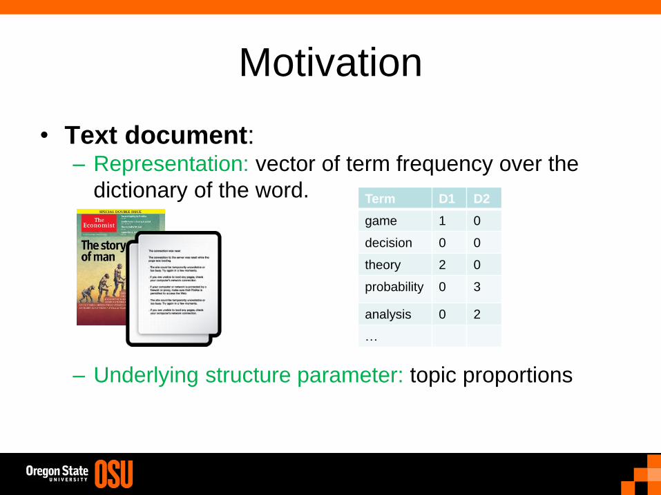
Motivation
• Text document: – Representation: vector of term frequency over the
dictionary of the word.
– Underlying structure parameter: topic proportions
Term D1 D2
game 1 0
decision 0 0
theory 2 0
probability 0 3
analysis 0 2
…
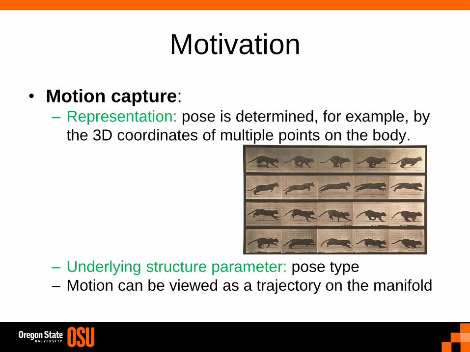
Motivation
• Motion capture: – Representation: pose is determined, for example, by
the 3D coordinates of multiple points on the body.
– Underlying structure parameter: pose type
– Motion can be viewed as a trajectory on the manifold

Motivation
• Microarray gene expression: – Representation: vector of gene expression values or
sequences of such vectors.
– Underlying structure parameter: correlated (or
dependent) gene groups

Motivation
Our main goal is to discover the underlying
structure of the data given the high
dimensional observations.
Real world datasets are highly nonlinear.
It is assumed that data lie on or close to a
very thin layer of a manifold embedded
into the high dimensional space.

Linear Dimension Reduction
• Common assumption:
data points lie on a low-
dimensional plane
• Properties:
•
•

Principle Component Analysis (PCA)
• Problem:
–
– Find the affine transformation
that maximizes the low-dimensional
transformed data variation:
– or equivalently
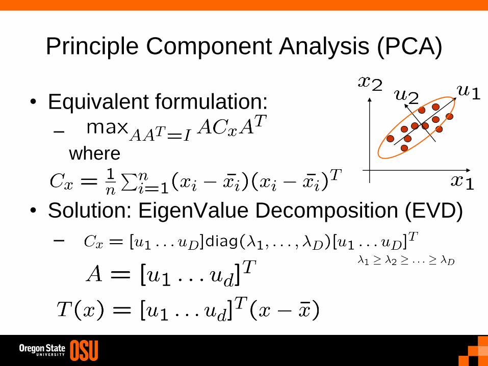
Principle Component Analysis (PCA)
• Equivalent formulation:
–
where
• Solution: EigenValue Decomposition (EVD)
–

Principle Component Analysis (PCA)
• PCA produces an affine transformation mapping the high
dimensional space into a low dimensional space.
• Distance:
• Spectral method
• Parametric: easily extends to new point
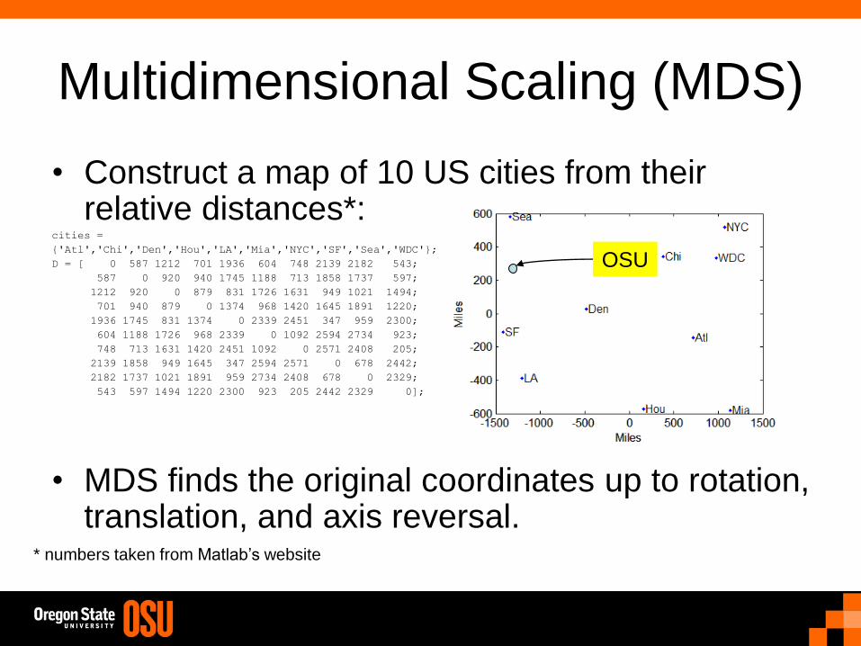
Multidimensional Scaling (MDS)
• Construct a map of 10 US cities from their relative distances*:
cities =
{'Atl','Chi','Den','Hou','LA','Mia','NYC','SF','Sea','WDC'};
D = [ 0 587 1212 701 1936 604 748 2139 2182 543;
587 0 920 940 1745 1188 713 1858 1737 597;
1212 920 0 879 831 1726 1631 949 1021 1494;
701 940 879 0 1374 968 1420 1645 1891 1220;
1936 1745 831 1374 0 2339 2451 347 959 2300;
604 1188 1726 968 2339 0 1092 2594 2734 923;
748 713 1631 1420 2451 1092 0 2571 2408 205;
2139 1858 949 1645 347 2594 2571 0 678 2442;
2182 1737 1021 1891 959 2734 2408 678 0 2329;
543 597 1494 1220 2300 923 205 2442 2329 0];
• MDS finds the original coordinates up to rotation, translation, and axis reversal.
OSU
* numbers taken from Matlab’s website
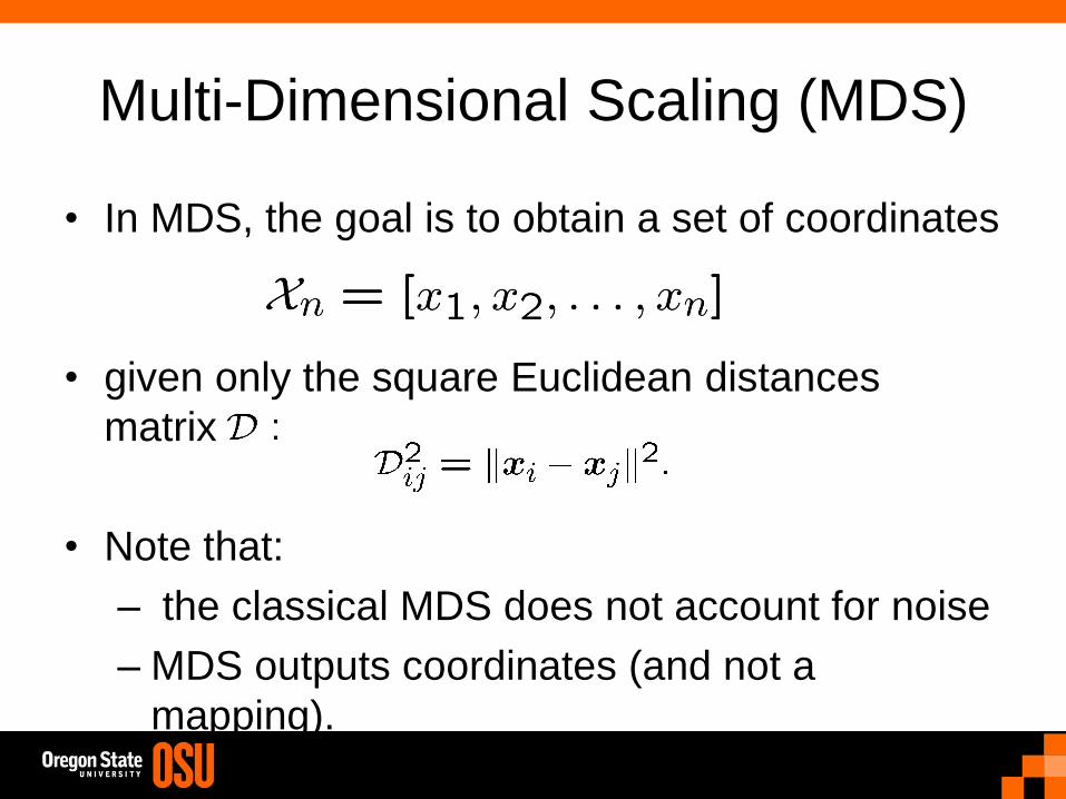
Multi-Dimensional Scaling (MDS)
• In MDS, the goal is to obtain a set of coordinates
• given only the square Euclidean distances
matrix
• Note that:
– the classical MDS does not account for noise
– MDS outputs coordinates (and not a
mapping).
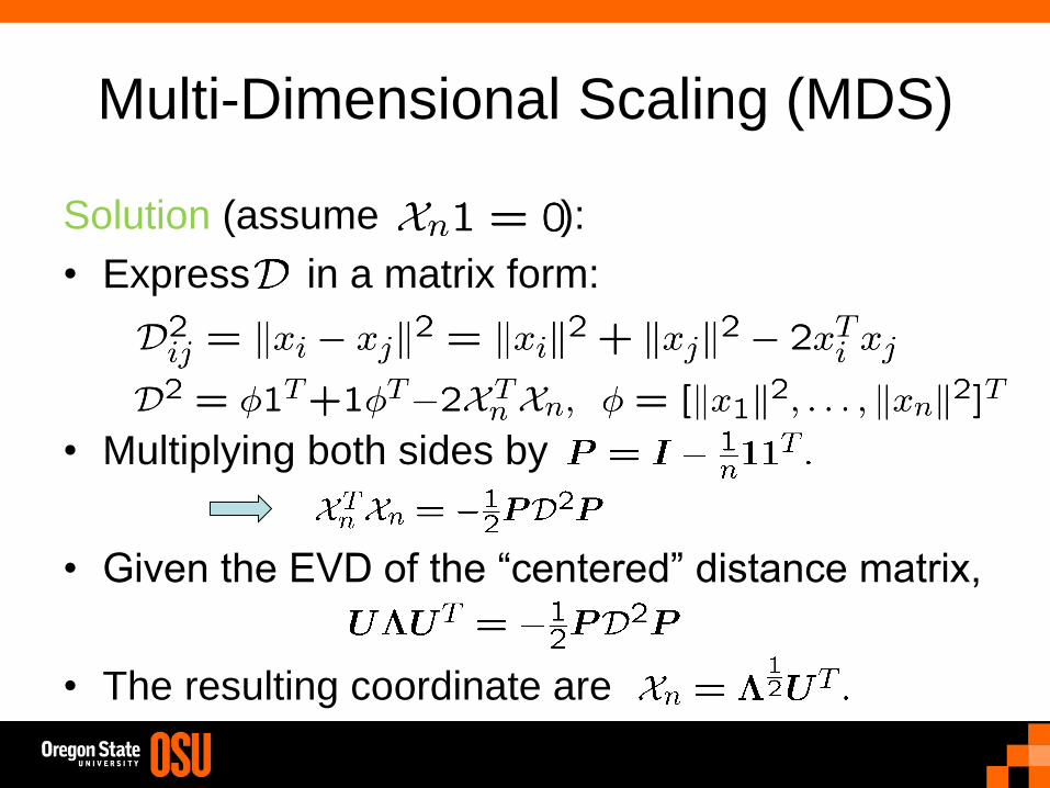
Multi-Dimensional Scaling (MDS)
Solution (assume ):
• Express in a matrix form:
• Multiplying both sides by
• Given the EVD of the “centered” distance matrix,
• The resulting coordinate are

Multi-Dimensional Scaling (MDS)
• Given a set of all distances finds coordinates:
• Non-parametric
• Requires all distances
• Generalizations:
– stress minimization (stress majorization)
– Euclidean distance matrix completion
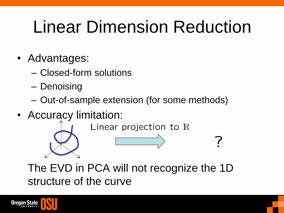
Linear Dimension Reduction
• Advantages:
– Closed-form solutions
– Denoising
– Out-of-sample extension (for some methods)
• Accuracy limitation:
The EVD in PCA will not recognize the 1D
structure of the curve

Manifold Learning
• Nomenclature:
– Manifold
– Local Coordinates
– Global Coordinates
– Tangent Plane
– Geodesics

• d-dimensional differentiable
manifold:
– Can be covered with open sets
which map (homomorphism) to
subsets of d-dimensional
Euclidean space
– Global mapping may not exist
• Tangent space:
Informal Introduction to
Manifolds
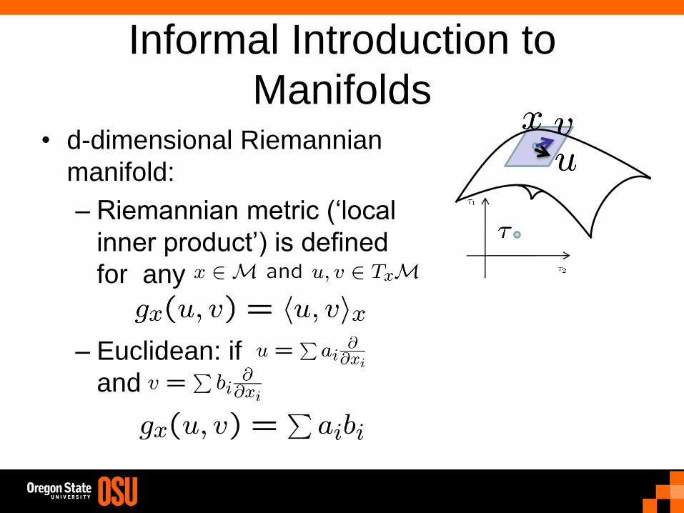
• d-dimensional Riemannian
manifold:
– Riemannian metric (‘local
inner product’) is defined
for any
– Euclidean: if
and
Informal Introduction to
Manifolds
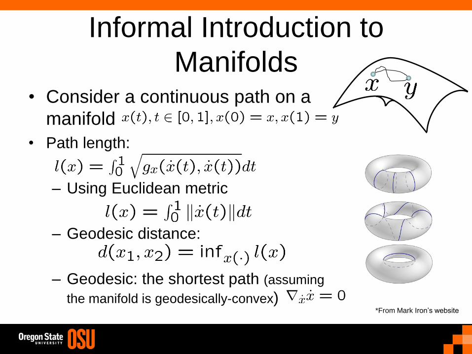
• Consider a continuous path on a
manifold
• Path length:
– Using Euclidean metric
– Geodesic distance:
– Geodesic: the shortest path (assuming
the manifold is geodesically-convex)
Informal Introduction to
Manifolds
*From Mark Iron’s website
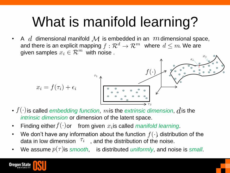
What is manifold learning? • A dimensional manifold is embedded in an dimensional space,
and there is an explicit mapping where . We are
given samples with noise .
• is called embedding function, is the extrinsic dimension, is the
intrinsic dimension or dimension of the latent space.
• Finding either or from given is called manifold learning.
• We don’t have any information about the function , distribution of the
data in low dimension , and the distribution of the noise.
• We assume is smooth, is distributed uniformly, and noise is small.
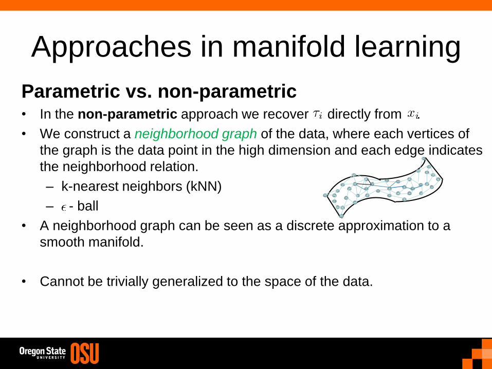
Approaches in manifold learning
Parametric vs. non-parametric • In the non-parametric approach we recover directly from .
• We construct a neighborhood graph of the data, where each vertices of
the graph is the data point in the high dimension and each edge indicates
the neighborhood relation.
– k-nearest neighbors (kNN)
– - ball
• A neighborhood graph can be seen as a discrete approximation to a
smooth manifold.
• Cannot be trivially generalized to the space of the data.

Approaches in manifold learning
Parametric vs. non-parametric
• In the parametric approach, we find the explicit mapping from the
given sample .
• Most of the approaches are probabilistic (latent factor modeling).
• We can generalize to the space of the data where there is no samples.
• There is no closed form solution for these algorithms and they prone to local
optimum.
• To have a coherent, single global low dimensional coordinate, we need to
take a further step and implement the process of coordinate alignment.
– Mixture of factor analyzers [Ghahramani et al’97].

Approaches in manifold learning
Isometric vs. non-isometric
• Isometric embedding is a mapping which preserves the metric.
• Intuitively, an isometry is a mapping that locally looks like a rotation plus translation,
thus preserving distances and angles among the vectors.
• ISOMAP [Tenenbaum et al’00], Maximum variance unfolding [Weinberger et al’04].
• Non-isometric embedding generally divides into two categories:
– Neighborhood preserving mapping which preserve the neighborhood relations among the
data points such as locally linear embedding (LLE), Laplacian eigenmap (LE) [Belkin et
al’03].
– Conformal mapping which is a mapping up to rotation, translation, and rescaling. It preserves
the angles among the data points as well as neighborhood relations such as conformal
ISOMAP [Sha et al’05].

Approaches in manifold learning • Global vs. local
– In the global preserving approaches, we preserve the global geometry
properties of the manifold such as geodesic distance (ISOMAP) [Tenenbaum
et al’00].
– Local preserving approaches rely on the fact that the surface of any manifold
can be locally approximated by its tangent space.
• Overlapping consensus of local geometry information can be used to find a single
global low dimensional embedding.
A B
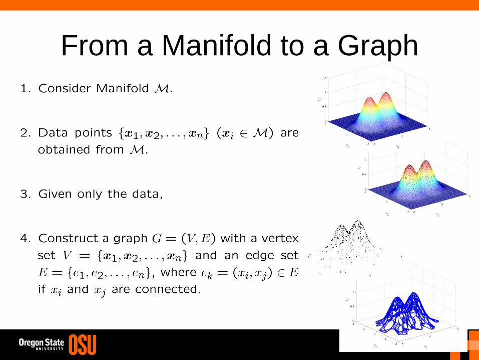
From a Manifold to a Graph
OSU EECS Colloquium (Fall'07)
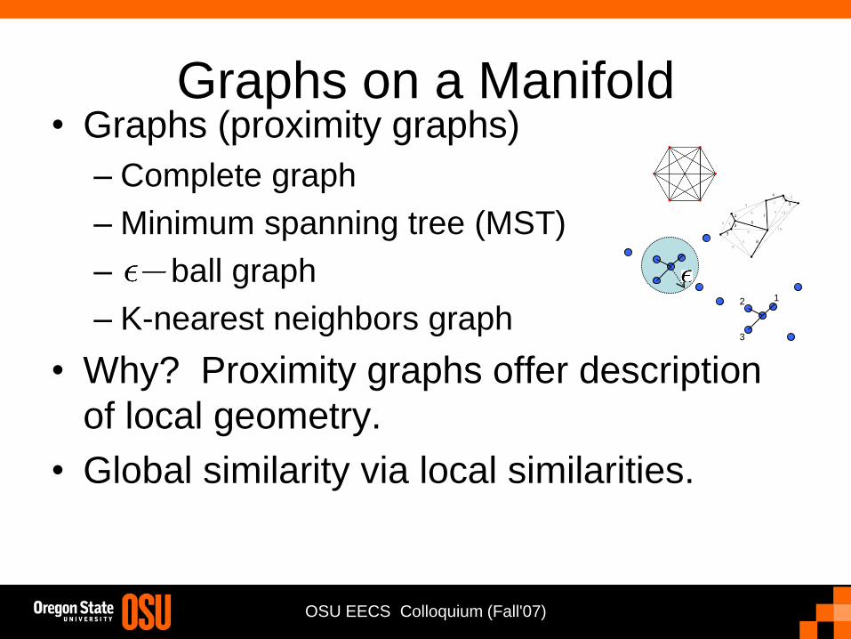
• Graphs (proximity graphs)
– Complete graph
– Minimum spanning tree (MST)
– ball graph
– K-nearest neighbors graph
• Why? Proximity graphs offer description
of local geometry.
• Global similarity via local similarities.
Graphs on a Manifold
1 2
3
Unweighted Graphs Representation
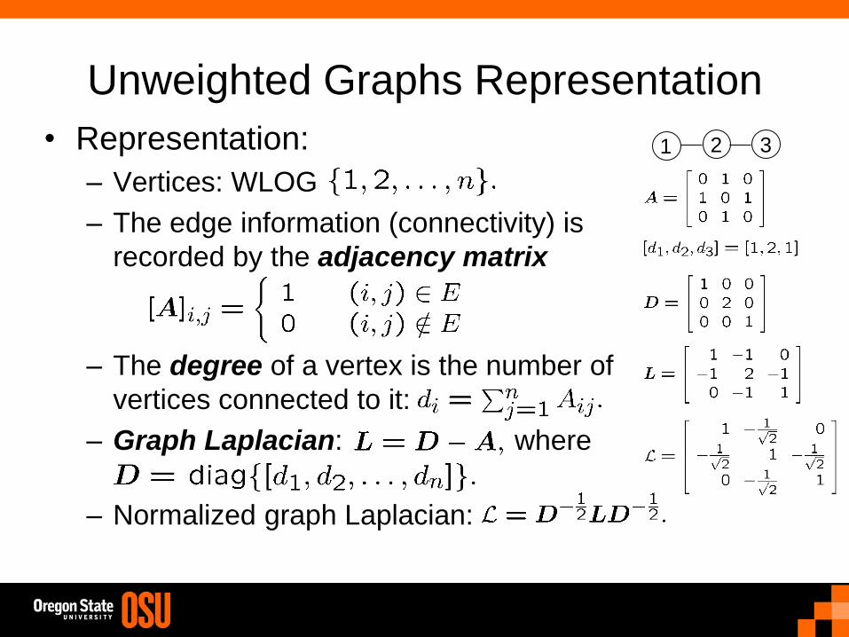
• Representation:
– Vertices: WLOG
– The edge information (connectivity) is
recorded by the adjacency matrix
– The degree of a vertex is the number of
vertices connected to it:
– Graph Laplacian: where
– Normalized graph Laplacian:
1 2 3
Weighted Graphs
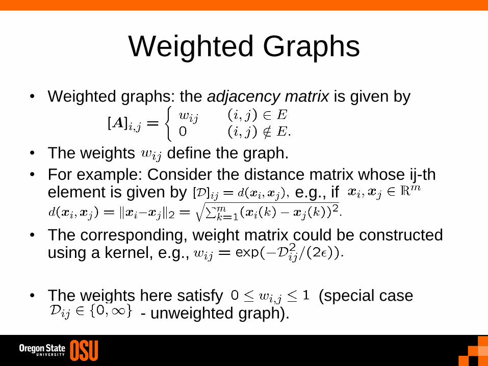
• Weighted graphs: the adjacency matrix is given by
• The weights define the graph.
• For example: Consider the distance matrix whose ij-th element is given by e.g., if
• The corresponding, weight matrix could be constructed using a kernel, e.g.,
• The weights here satisfy (special case - unweighted graph).
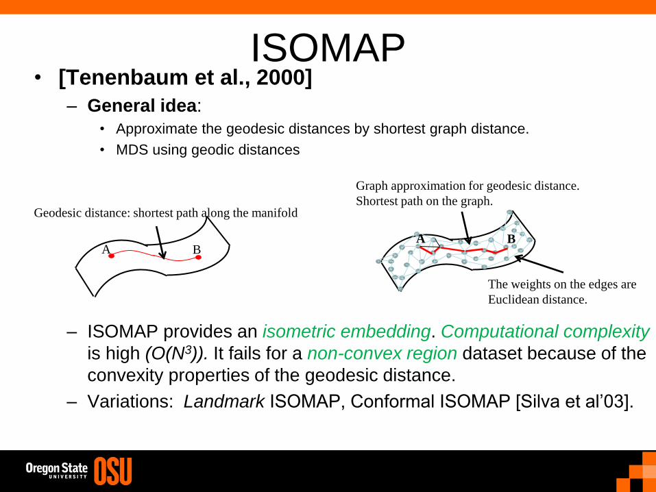
ISOMAP • [Tenenbaum et al., 2000]
– General idea:
• Approximate the geodesic distances by shortest graph distance.
• MDS using geodic distances
– ISOMAP provides an isometric embedding. Computational complexity
is high (O(N3)). It fails for a non-convex region dataset because of the
convexity properties of the geodesic distance.
– Variations: Landmark ISOMAP, Conformal ISOMAP [Silva et al’03].
A B
Geodesic distance: shortest path along the manifold
A B
Graph approximation for geodesic distance.
Shortest path on the graph.
The weights on the edges are
Euclidean distance.

ISOMAP • [Tenenbaum et al., 2000]
• Algorithm:
– Construct a neighborhood graph
– Construct a distance matrix
– Find the shortest path between every i and j (e.g. using Floyd-
Marshall) and construct a new distance matrix such that is the
length of the shortest path between i and j.
– Apply MDS to matrix to find coordinates
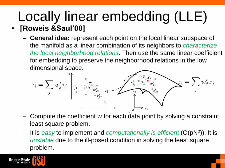
Locally linear embedding (LLE) • [Roweis &Saul’00]
– General idea: represent each point on the local linear subspace of
the manifold as a linear combination of its neighbors to characterize
the local neighborhood relations. Then use the same linear coefficient
for embedding to preserve the neighborhood relations in the low
dimensional space.
– Compute the coefficient w for each data point by solving a constraint
least square problem.
– It is easy to implement and computationally is efficient (O(pN2)). It is
unstable due to the ill-posed condition in solving the least square
problem.
– Variation: Modified LLE [Zhang et al’07].
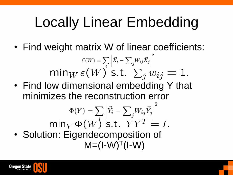
Locally Linear Embedding
• Find weight matrix W of linear coefficients:
• Find low dimensional embedding Y that minimizes the reconstruction error
• Solution: Eigendecomposition of M=(I-W)T(I-W)
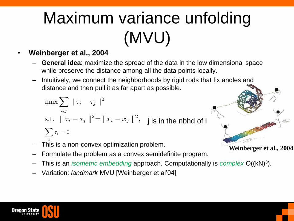
Maximum variance unfolding
(MVU) • Weinberger et al., 2004
– General idea: maximize the spread of the data in the low dimensional space
while preserve the distance among all the data points locally.
– Intuitively, we connect the neighborhoods by rigid rods that fix angles and
distance and then pull it as far apart as possible.
– This is a non-convex optimization problem.
– Formulate the problem as a convex semidefinite program.
– This is an isometric embedding approach. Computationally is complex O((kN)3).
– Variation: landmark MVU [Weinberger et al’04]
Weinberger et al., 2004
j is in the nbhd of i
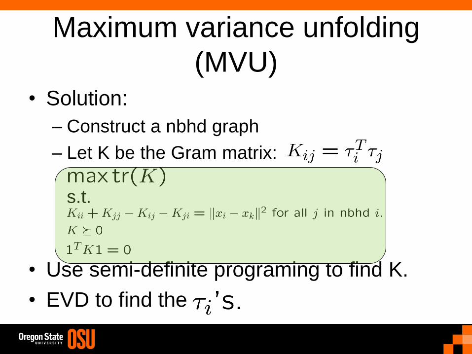
Maximum variance unfolding
(MVU) • Solution:
– Construct a nbhd graph
– Let K be the Gram matrix:
s.t.
• Use semi-definite programing to find K.
• EVD to find the

Laplacian eigenmaps (LE) • Belkin et al., 2003
– General idea: minimize the norm of Laplace-Beltrami operator on the
manifold
– measures how far apart maps nearby points.
– Avoid the trivial solution of f = const.
– The Laplacian-Beltrami operator can be approximated by Laplacian of the
neighborhood graph with appropriate weights.
– Construct the Laplacian matrix L=D-W.
– can be approximated by its discrete equivalent:
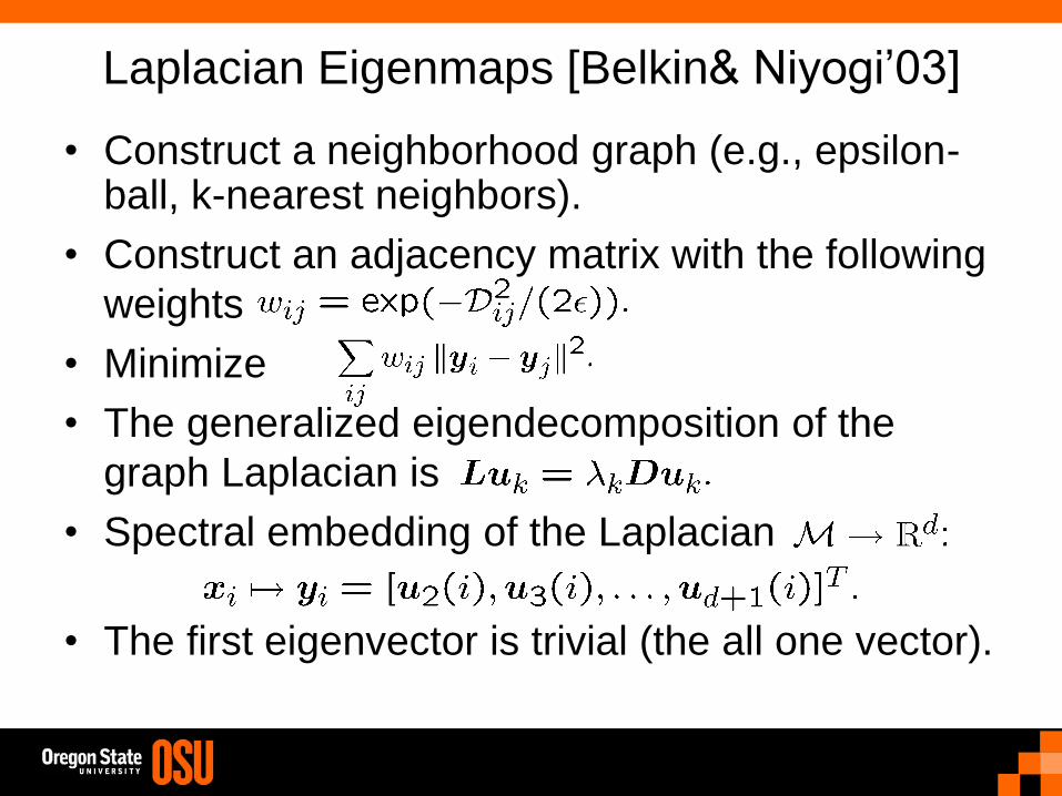
Laplacian Eigenmaps [Belkin& Niyogi’03]
• Construct a neighborhood graph (e.g., epsilon-ball, k-nearest neighbors).
• Construct an adjacency matrix with the following
weights
• Minimize
• The generalized eigendecomposition of the
graph Laplacian is
• Spectral embedding of the Laplacian
• The first eigenvector is trivial (the all one vector).
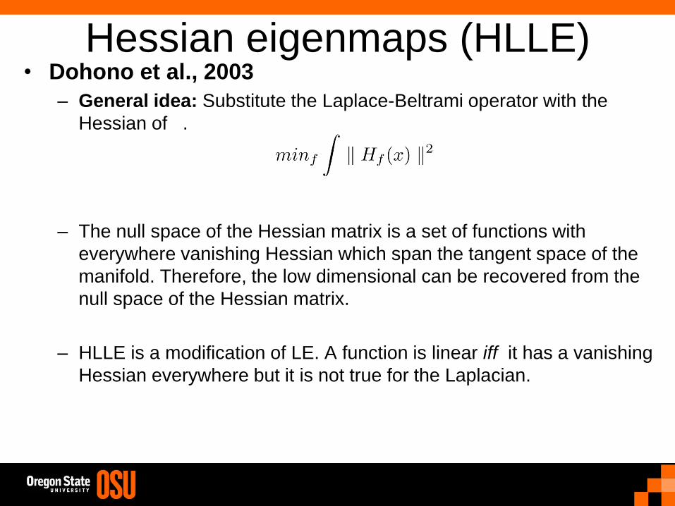
Hessian eigenmaps (HLLE) • Dohono et al., 2003
– General idea: Substitute the Laplace-Beltrami operator with the
Hessian of .
– The null space of the Hessian matrix is a set of functions with
everywhere vanishing Hessian which span the tangent space of the
manifold. Therefore, the low dimensional can be recovered from the
null space of the Hessian matrix.
– HLLE is a modification of LE. A function is linear iff it has a vanishing
Hessian everywhere but it is not true for the Laplacian.

Local tangent space alignment • Every smooth manifold can be constructed locally by its tangent plane.
• Taylor series expansion of the embedding function in the local
neighborhood of can be given as following:
• We are given samples from the embedded manifold with
noise therefore,
• For an arbitrary point and its local neighbor and in the absence of
the noise, we can write:
• If we have the explicit mapping therefore we can discover from
the given .

Local tangent space alignment
,
where
PCA
Alignment:
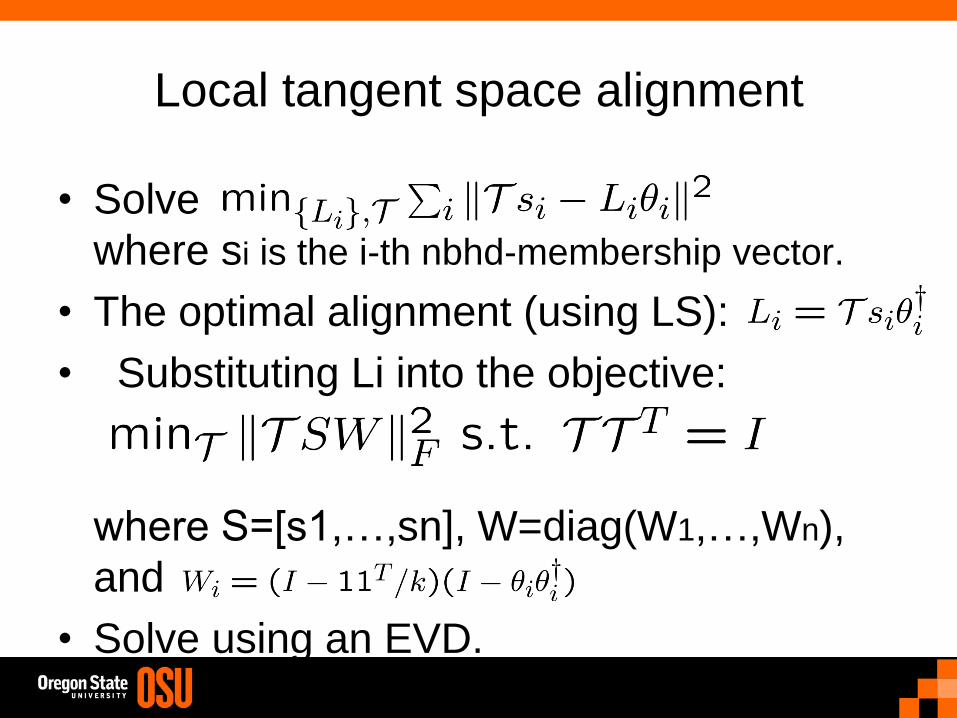
• Solve
where si is the i-th nbhd-membership vector.
• The optimal alignment (using LS):
• Substituting Li into the objective:
where S=[s1,…,sn], W=diag(W1,…,Wn),
and
• Solve using an EVD.
Local tangent space alignment

Other Nonlinear Methods
• Kohonen Self-Organizing Map
[Kohonen1990]
• Kernel PCA [Mika et. Al.’99]
• Neural nets

Probabilistic Approaches
• Based on a probabilistic model relating the
high dimensional data and the low
dimensional data.
• Examples: SNE, Probabilistic PCA, MFA

Stochastic Neighbor Embedding
[Hinton&Roweis’02] • Construct the probability that i
will choose j as its neighbor
p(j|i):
• For the low-dimensional
embedding define:
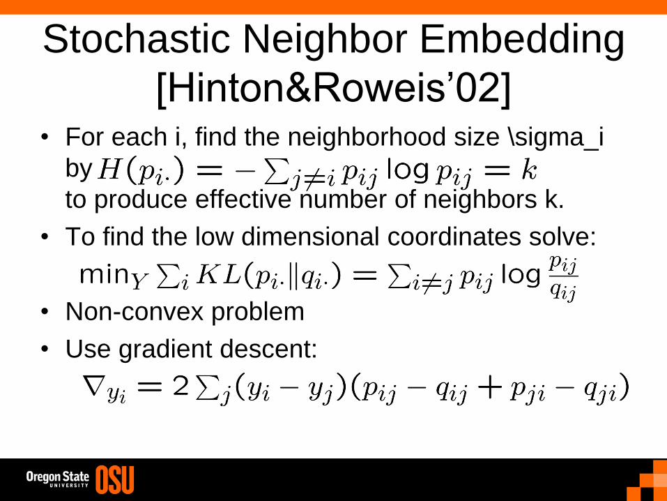
Stochastic Neighbor Embedding
[Hinton&Roweis’02] • For each i, find the neighborhood size \sigma_i
by
to produce effective number of neighbors k.
• To find the low dimensional coordinates solve:
• Non-convex problem
• Use gradient descent:
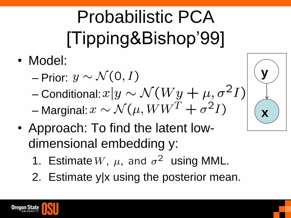
Probabilistic PCA
[Tipping&Bishop’99] • Model:
– Prior:
– Conditional:
– Marginal:
• Approach: To find the latent low-
dimensional embedding y:
1. Estimate using MML.
2. Estimate y|x using the posterior mean.
y
x
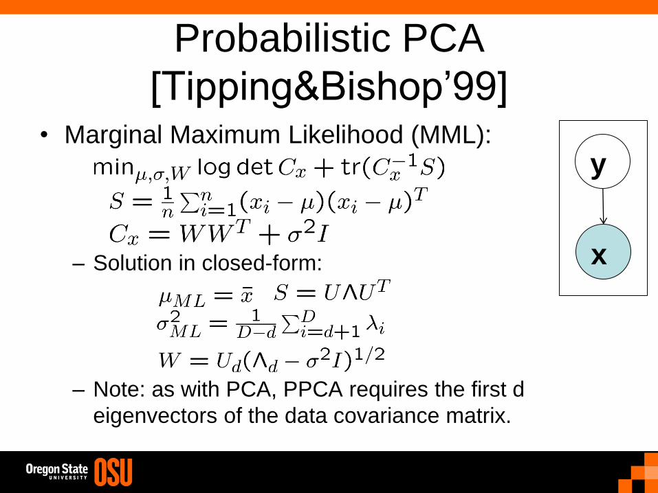
Probabilistic PCA
[Tipping&Bishop’99] • Marginal Maximum Likelihood (MML):
– Solution in closed-form:
– Note: as with PCA, PPCA requires the first d
eigenvectors of the data covariance matrix.
y
x
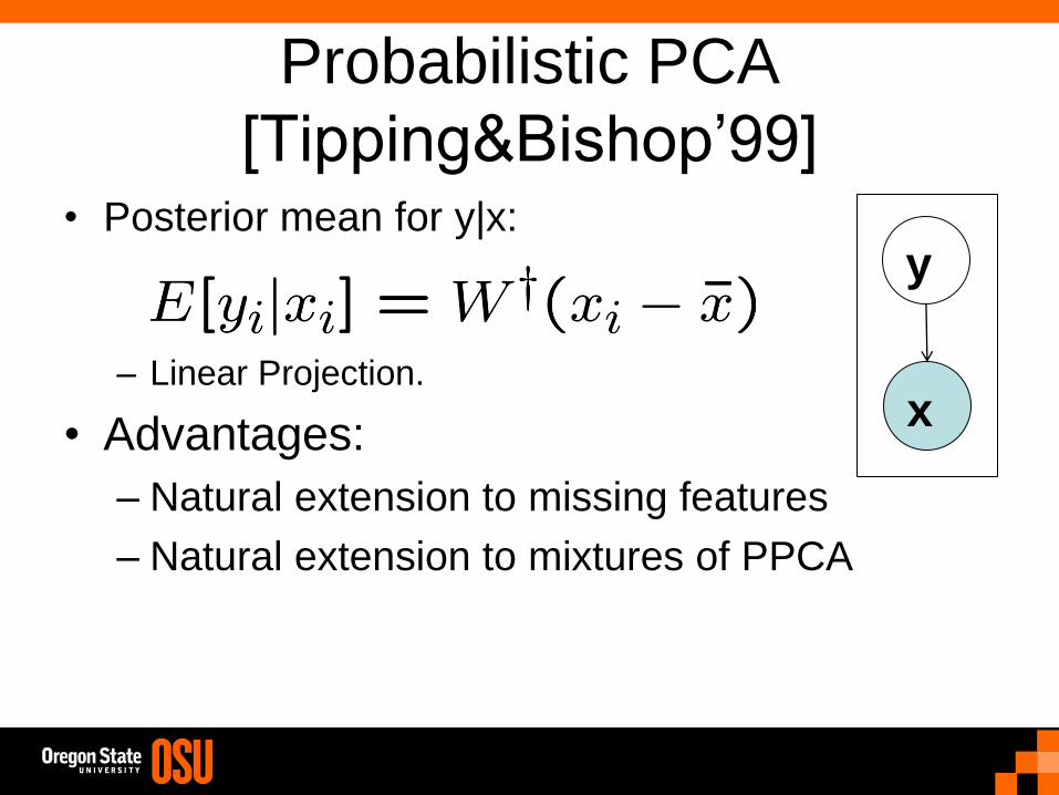
Probabilistic PCA
[Tipping&Bishop’99] • Posterior mean for y|x:
– Linear Projection.
• Advantages:
– Natural extension to missing features
– Natural extension to mixtures of PPCA
y
x
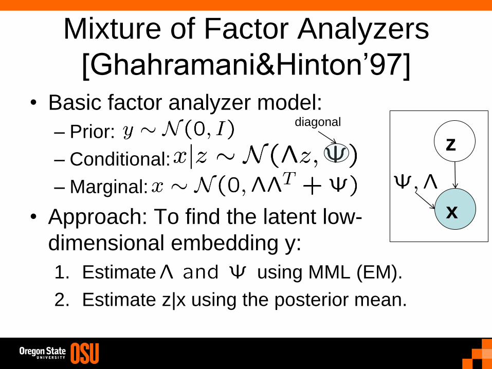
Mixture of Factor Analyzers
[Ghahramani&Hinton’97] • Basic factor analyzer model:
– Prior:
– Conditional:
– Marginal:
• Approach: To find the latent low-
dimensional embedding y:
1. Estimate using MML (EM).
2. Estimate z|x using the posterior mean.
diagonal
z
x
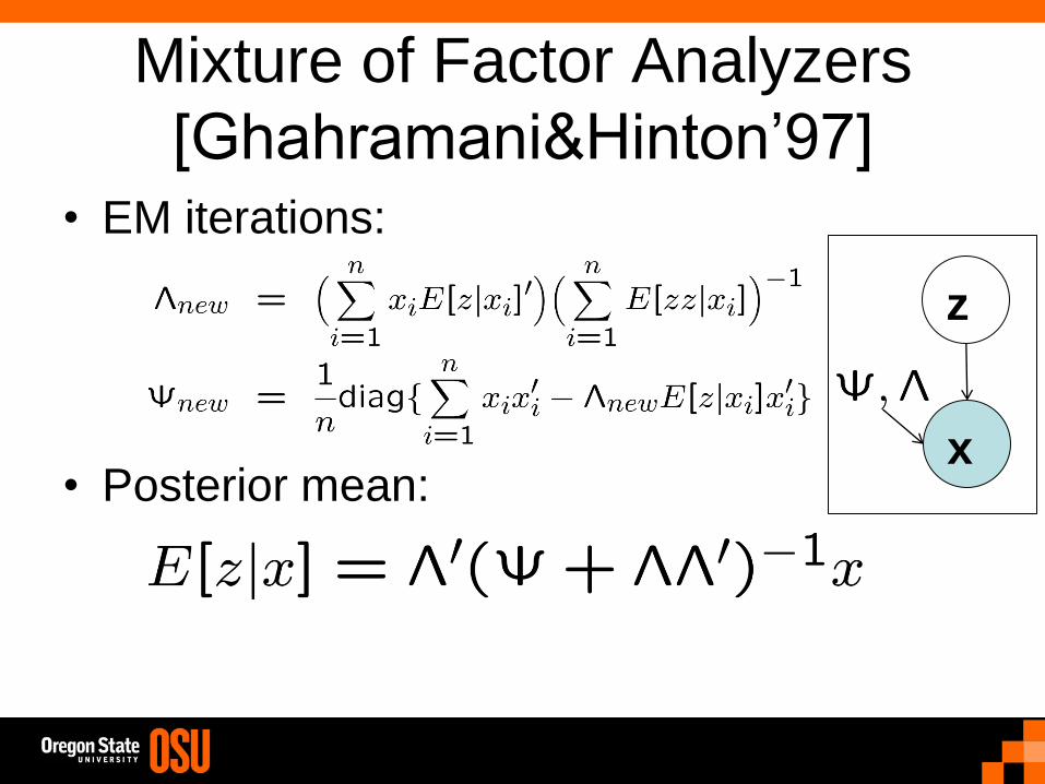
Mixture of Factor Analyzers
[Ghahramani&Hinton’97] • EM iterations:
• Posterior mean:
z
x
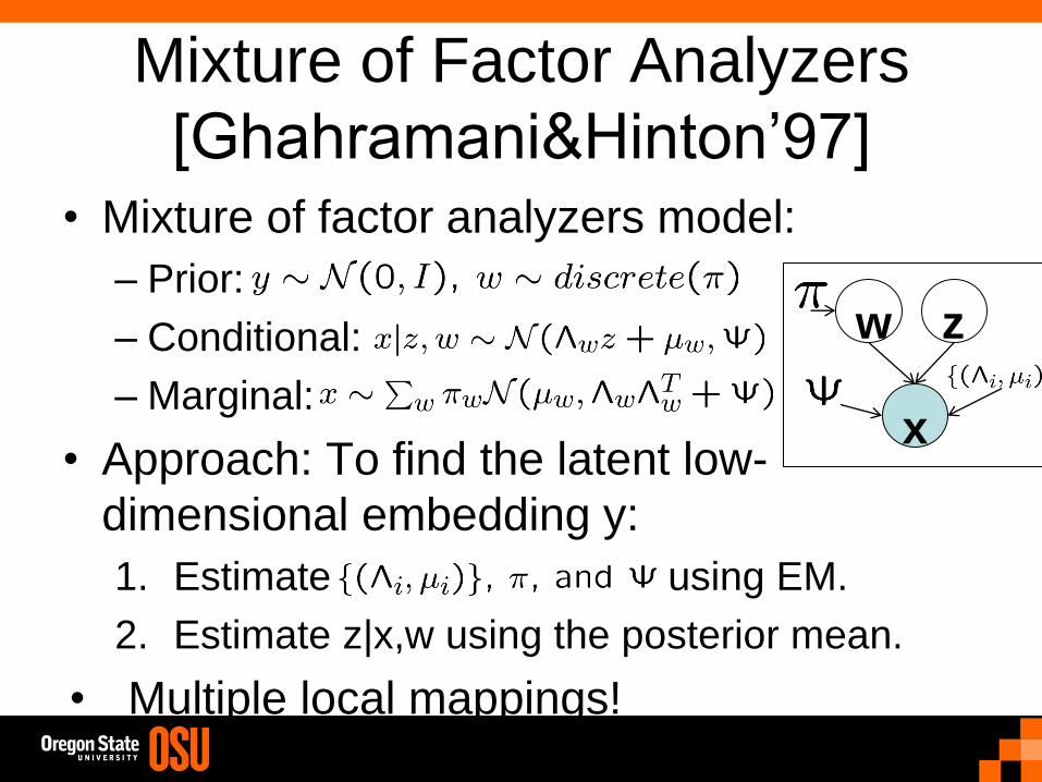
Mixture of Factor Analyzers
[Ghahramani&Hinton’97] • Mixture of factor analyzers model:
– Prior:
– Conditional:
– Marginal:
• Approach: To find the latent low-
dimensional embedding y:
1. Estimate using EM.
2. Estimate z|x,w using the posterior mean.
• Multiple local mappings!
z
x
w
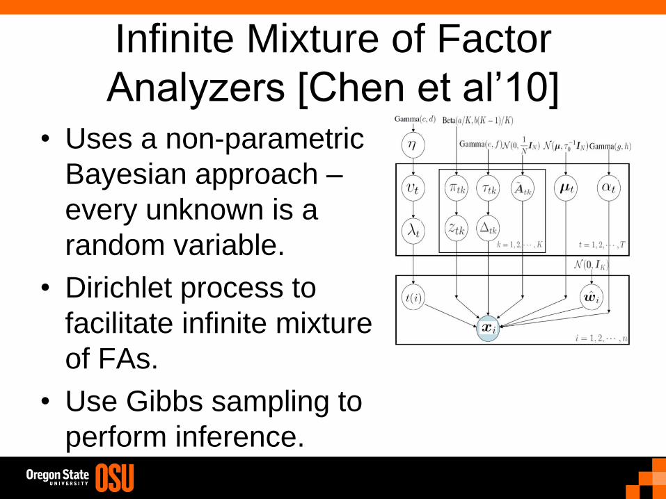
Infinite Mixture of Factor
Analyzers [Chen et al’10] • Uses a non-parametric
Bayesian approach –
every unknown is a
random variable.
• Dirichlet process to
facilitate infinite mixture
of FAs.
• Use Gibbs sampling to
perform inference.
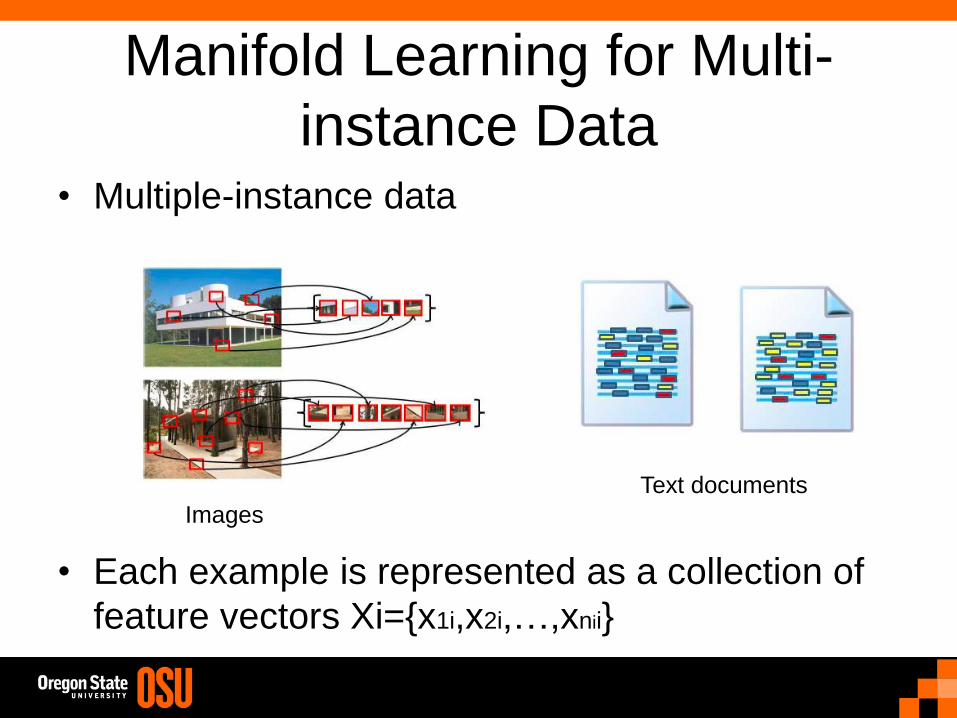
Manifold Learning for Multi-
instance Data • Multiple-instance data
• Each example is represented as a collection of
feature vectors Xi={x1i,x2i,…,xnii}
Text documents
Images
OSU EECS Colloquium (Fall'07)
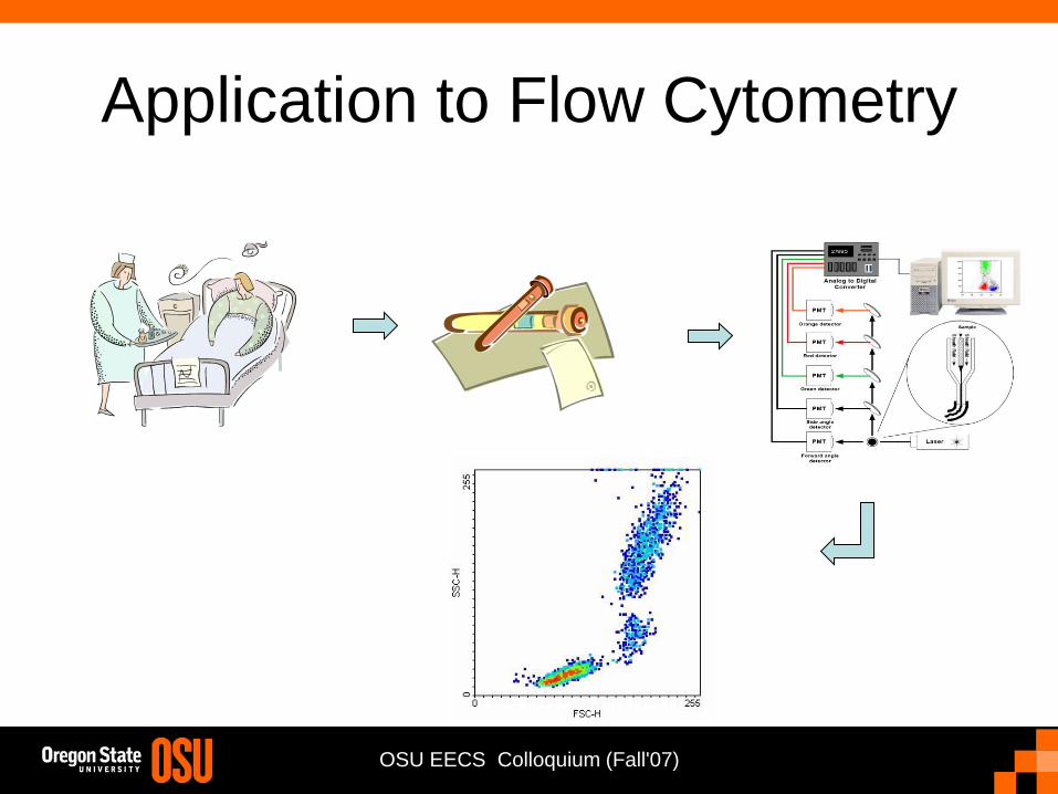
Application to Flow Cytometry
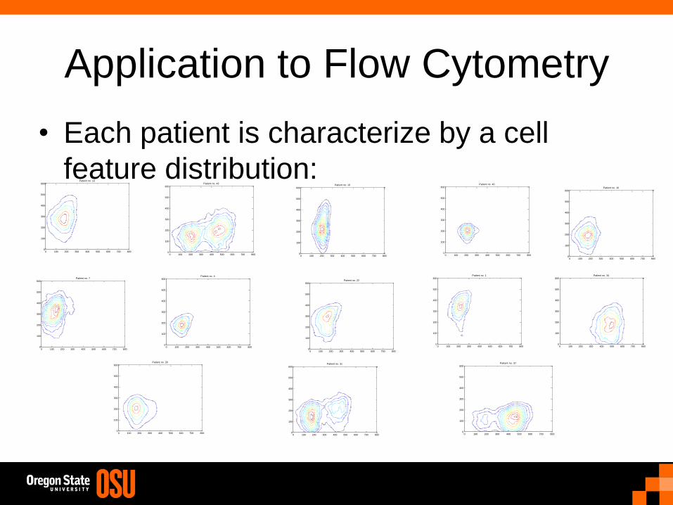
Application to Flow Cytometry
• Each patient is characterize by a cell
feature distribution:
Patient no. 7
0 100 200 300 400 500 600 700 8000
100
200
300
400
500
600
Patient no. 13
0 100 200 300 400 500 600 700 8000
100
200
300
400
500
600
Patient no. 16
0 100 200 300 400 500 600 700 8000
100
200
300
400
500
600
Patient no. 43
0 100 200 300 400 500 600 700 8000
100
200
300
400
500
600
Patient no. 34
0 100 200 300 400 500 600 700 8000
100
200
300
400
500
600
Patient no. 40
0 100 200 300 400 500 600 700 8000
100
200
300
400
500
600
Patient no. 37
0 100 200 300 400 500 600 700 8000
100
200
300
400
500
600Patient no. 31
0 100 200 300 400 500 600 700 8000
100
200
300
400
500
600
Patient no. 1
0 100 200 300 400 500 600 700 8000
100
200
300
400
500
600Patient no. 4
0 100 200 300 400 500 600 700 8000
100
200
300
400
500
600Patient no. 22
0 100 200 300 400 500 600 700 8000
100
200
300
400
500
600
Patient no. 28
0 100 200 300 400 500 600 700 8000
100
200
300
400
500
600
Patient no. 10
0 100 200 300 400 500 600 700 8000
100
200
300
400
500
600
Manifold Learning for Multi-
instance Data • How can manifold learning be extended to
learning embedding for objects that are
not represented as vectors?
• To determine neighborhood graphs, a
distance is required. D(Xi,Xj)=?
• How can we construct tangent planes?
• Approach: treat the i-th ‘bag’ an iid draw
from a generative model f(x|θi)

Information Geometry
• Consider the manifold of densities M:
• Use the Fisher information metric as a
Riemannian metric for the manifold:
The metric defines an inner product, which
allows us to compute distances.
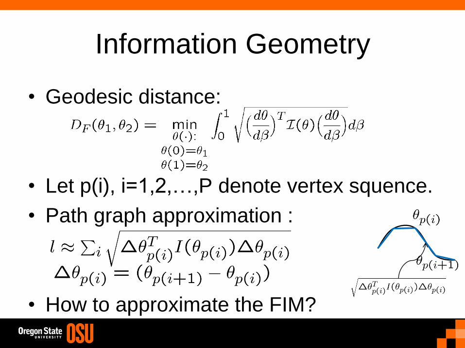
Information Geometry
• Geodesic distance:
• Let p(i), i=1,2,…,P denote vertex squence.
• Path graph approximation :
• How to approximate the FIM?
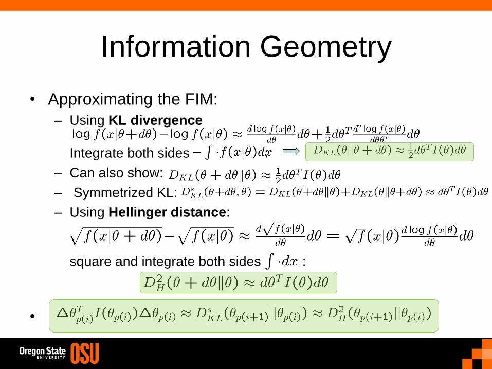
Information Geometry
• Approximating the FIM:
– Using KL divergence
Integrate both sides :
– Can also show:
– Symmetrized KL:
– Using Hellinger distance:
square and integrate both sides :
•
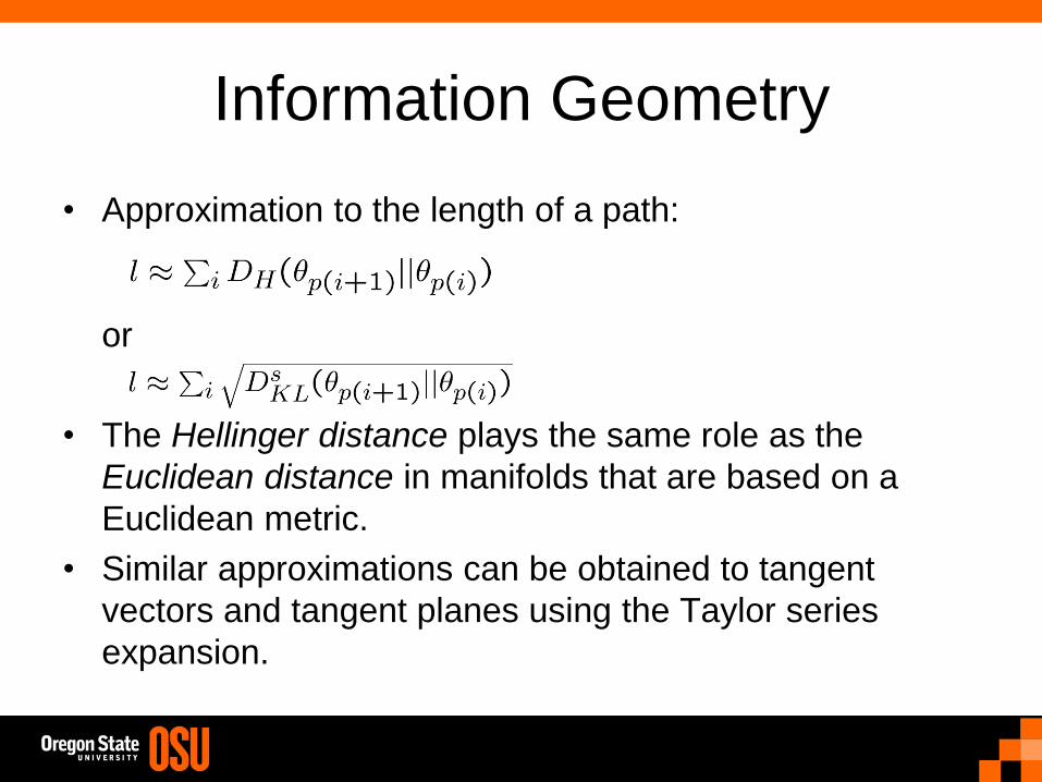
Information Geometry
• Approximation to the length of a path:
or
• The Hellinger distance plays the same role as the
Euclidean distance in manifolds that are based on a
Euclidean metric.
• Similar approximations can be obtained to tangent
vectors and tangent planes using the Taylor series
expansion.
Experimental Setting
• Unsupervised learning – clustering.
• 43 Patients: 23 CLL patients and 20 MCL patients.
• For both diseases, analysis is of just the lymphocytes.
• Varying number of cells (around 5000-6000) per patient are recorded.
• Testing ten different six-dimensional marker combination data samples.
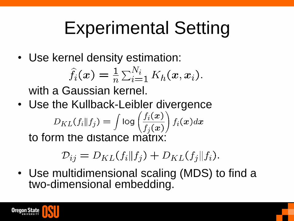
Experimental Setting
• Use kernel density estimation: with a Gaussian kernel.
• Use the Kullback-Leibler divergence to form the distance matrix:
• Use multidimensional scaling (MDS) to find a two-dimensional embedding.

Obtaining the PDFs
Patient 1: Scatter plot
of FMC7 vs. CD23 Patient 1: density estimate
• Actual density estimation was performed for the six-variate density.
-40 -30 -20 -10 0 10 20 30 40 50 -50
-40
-30
-20
-10
0
10
20
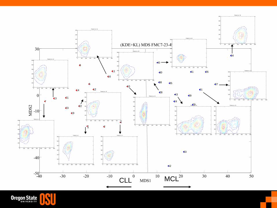
30 (KDE+KL) MDS FMC7-23-45
MDS1
MD
S2
1 2
3
4
5
6
7
8
9
10
11
12
13
14
15 16
17
18
19
20
21
22 23
24
25
26
27
28
29
30
31
32
33
34
35 36 37
38
39
40
41
42
43
Patient no. 7
0 100 200 300 400 500 600 700 8000
100
200
300
400
500
600
Patient no. 13
0 100 200 300 400 500 600 700 8000
100
200
300
400
500
600
Patient no. 16
0 100 200 300 400 500 600 700 8000
100
200
300
400
500
600
Patient no. 43
0 100 200 300 400 500 600 700 8000
100
200
300
400
500
600
Patient no. 34
0 100 200 300 400 500 600 700 8000
100
200
300
400
500
600
Patient no. 40
0 100 200 300 400 500 600 700 8000
100
200
300
400
500
600
Patient no. 37
0 100 200 300 400 500 600 700 8000
100
200
300
400
500
600
Patient no. 31
0 100 200 300 400 500 600 700 8000
100
200
300
400
500
600
Patient no. 1
0 100 200 300 400 500 600 700 8000
100
200
300
400
500
600Patient no. 4
0 100 200 300 400 500 600 700 8000
100
200
300
400
500
600
Patient no. 22
0 100 200 300 400 500 600 700 8000
100
200
300
400
500
600
Patient no. 28
0 100 200 300 400 500 600 700 8000
100
200
300
400
500
600
Patient no. 10
0 100 200 300 400 500 600 700 8000
100
200
300
400
500
600
MCL CLL
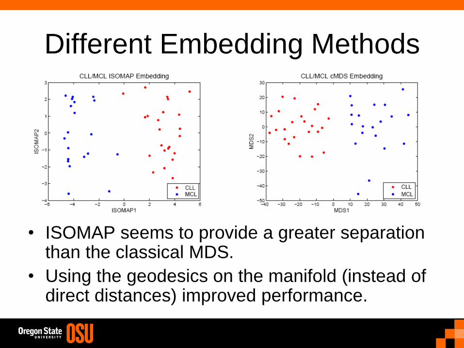
Different Embedding Methods
• ISOMAP seems to provide a greater separation than the classical MDS.
• Using the geodesics on the manifold (instead of direct distances) improved performance.
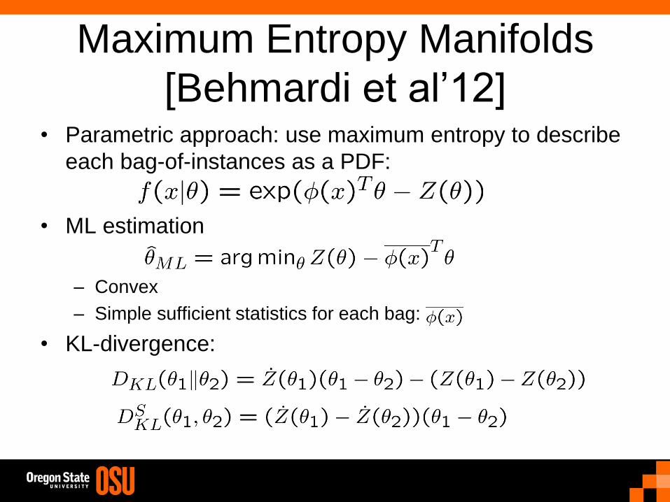
Maximum Entropy Manifolds
[Behmardi et al’12] • Parametric approach: use maximum entropy to describe
each bag-of-instances as a PDF:
• ML estimation
– Convex
– Simple sufficient statistics for each bag:
• KL-divergence:

Maximum Entropy Manifolds
[Behmardi et al’12] • Experiment:
• Corel 1000 data set
• Each image is divided in to blocks
• Use PCA to represent each block using a low-
dimensional vector.

Maximum Entropy Manifolds
[Behmardi et al’12] • Accuracy:
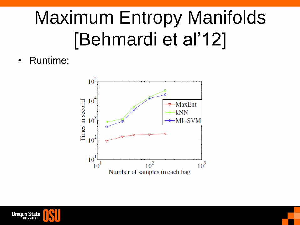
Maximum Entropy Manifolds
[Behmardi et al’12] • Runtime:

Conclusion
• Introduced linear and nonlinear dimension
reduction
• Presented manifold and manifold learning
techniques
• Common tools
• Geometric vs. probabilistic
• Generalization to probability spaces
List of references for manifold learning
1 Algorithms
1.1 Graph-based approach
1.1.1 Globally Embedding
1. A global geometric framework for nonlinear dimensionality reduction (ISOMAP) [1]
2. Maximum variance unfolding (MVU) [2, 3]
3. Diffusion maps [4]
4. Graph approximations to geodesics on embedded manifolds [5]
5. Unsupervised learning of curved manifolds[6]
1.1.2 Locally Embedding
1. Locally Linear Embedding (LLE) [7, 8]
2. Laplacian eigenmaps [9]
3. Hessian eigenmpas [10]
4. Local tangent space alignment (LTSA) [11]
5. Manifold charting [12]
6. Two-Manifold Problems with Applications to Nonlinear System Identification [13]
7. Robust Multiple Manifolds Structure Learning [14]
1

1.1.3 Variations of global and local embedding
1. Conformal Isomap Embedding [15]
2. Graph laplacian regularization for large-scale semidefinite programming [16]
3. Modified locally linear embedding [17]
4. Colored maximum variance unfolding [18]
5. Grouping and dimensionality reduction by locally linear embedding [19]
6. Sparse multidimensional scaling using landmark points [20]
7. Improved local coordinate coding using local tangents [21]
1.2 Probabilistic approach
1. Mixture of factor analysis (MFA) [22]
2. Stochastic neighborhood embedding (SNE) [23]
3. The generative topographic mapping (GTM) [24]
4. Probabilistic principal component analysis [25]
5. Global coordinate of local linear models [26]
6. Automatic alignment of local representations [27]
7. Coordinating principal component analysis [28]
1.3 Non-probabilistic approach
1. Multilayer autoencoders [29]
2. The self-organizing map [30]
3. Sammon mapping [31]
4. Kernel PCA [32]
5. Principal curves [33]
6. A variational approach to recovering a manifold from sample points [34]
2
7. Out-of-sample extensions for LLE, Isomap, MDS, Eigenmaps, and spectral clustering [35]
8. Continuous nonlinear dimensionality reduction by kernel eigenmaps [36]
9. Learning eigenfunctions links spectral embedding and kernel PCA [37]
10. Sparse manifold clustering and embedding [38]
1.4 Supervised and semisupervised manifold learning
1. Vector-valued manifold regularization [39]
2. Multiple instance learning with manifold bags [40]
3. The manifold tangent classifier [41]
2 Applications
1. Maximum covariance unfolding: Manifold learning for bimodal data [42]
2. Humans learn using manifolds, reluctantly [43]
3. Learning multiple tasks using manifold regularization [44]
4. Online learning in the manifold of low-rank matrices [45]
5. Manifold Precis: An Annealing Technique for Diverse Sampling of Manifolds [46]
6. Nonlinear dimensionality reduction as information retrieval [47]
7. Information retrieval perspective to nonlinear dimensionality reduction for data visualization [48]
8. Unified Locally Linear Embedding and Linear Discriminant Analysis Algorithm (ULLELDA) forFace Recognition [49]
9. Generative modeling for continuous non-linearly embedded visual inference [50]
10. Manifold learning and applications in recognition [51]
11. Graph-driven features extraction from microarray data using diffusion kernels and kernel CCA [52]
12. Manifold based analysis of facial expression [53]
13. A dimensionality reduction approach to modeling protein flexibility [54]
3
14. Face recognition from face motion manifolds using robust kernel resistor-average distance [55]
15. Coloring of DT-MRI fiber traces using Laplacian eigenmaps [56]
16. Freeway traffic stream modeling based on principal curves and its analysis [57]
17. Super-resolution through neighbor embedding [58]
3 Dimension Estimation
1. Manifold-adaptive dimension estimation [59]
2. Towards manifold-adaptive learning [60]
3. Maximum likelihood estimation of intrinsic dimension [61]
4. Manifold learning using Euclidean k-nearest neighbor graphs [62]
5. An intrinsic dimensionality estimator from near-neighbor information [63]
6. Intrinsic dimension estimation of manifolds by incising balls [64]
7. Intrinsic dimension estimation by maximum likelihood in probabilistic PCA [65]
References
[1] J.B. Tenenbaum, V. De Silva, and J.C. Langford, “A global geometric framework for nonlineardimensionality reduction,” Science, vol. 290, no. 5500, pp. 2319–2323, 2000.
[2] K.Q. Weinberger and L.K. Saul, “Unsupervised learning of image manifolds by semidefinite pro-gramming,” in Computer Vision and Pattern Recognition, 2004. CVPR 2004. Proceedings of the2004 IEEE Computer Society Conference on. IEEE, 2004, vol. 2, pp. II–988.
[3] K.Q. Weinberger, F. Sha, and L.K. Saul, “Learning a kernel matrix for nonlinear dimensionalityreduction,” in Proceedings of the twenty-first international conference on Machine learning. ACM,2004, p. 106.
[4] R.R. Coifman and S. Lafon, “Diffusion maps,” Applied and Computational Harmonic Analysis, vol.21, no. 1, pp. 5–30, 2006.
[5] M. Bernstein, V. De Silva, J.C. Langford, and J.B. Tenenbaum, “Graph approximations to geodesicson embedded manifolds,” Tech. Rep., Technical report, Department of Psychology, Stanford Uni-versity, 2000.
4
[6] V. de Silva and J. Tenenbaum, “Unsupervised learning of curved manifolds,” in Proceedings of theMSRI workshop on nonlinear estimation and classification, 2002.
[7] S.T. Roweis and L.K. Saul, “Nonlinear dimensionality reduction by locally linear embedding,”Science, vol. 290, no. 5500, pp. 2323–2326, 2000.
[8] L.K. Saul and S.T. Roweis, “An introduction to locally linear embedding,” unpublished. Availableat: http://www. cs. toronto. edu/˜ roweis/lle/publications. html, 2000.
[9] M. Belkin and P. Niyogi, “Laplacian eigenmaps and spectral techniques for embedding and cluster-ing,” Advances in neural information processing systems, vol. 14, pp. 585–591, 2001.
[10] D.L. Donoho and C. Grimes, “Hessian eigenmaps: Locally linear embedding techniques for high-dimensional data,” Proceedings of the National Academy of Sciences of the United States of America,vol. 100, no. 10, pp. 5591, 2003.
[11] T. Zhang, J. Yang, D. Zhao, and X. Ge, “Linear local tangent space alignment and application toface recognition,” Neurocomputing, vol. 70, no. 7, pp. 1547–1553, 2007.
[12] M. Brand, “Charting a manifold,” Advances in neural information processing systems, pp. 985–992,2003.
[13] B. Boots and G. Gordon, “Two-manifold problems with applications to nonlinear system identifica-tion,” ICML2012, 2012.
[14] D. Gong, X. Zhao, and G. Medioni, “Robust multiple manifolds structure learning,” ICML2012,2012.
[15] V. Silva and J.B. Tenenbaum, “Global versus local methods in nonlinear dimensionality reduction,”Advances in neural information processing systems, vol. 15, pp. 705–712, 2003.
[16] K.Q. Weinberger, F. Sha, Q. Zhu, and L.K. Saul, “Graph laplacian regularization for large-scalesemidefinite programming,” Advances in neural information processing systems, vol. 19, pp. 1489,2007.
[17] Z. Zhang and J. Wang, “Mlle: Modified locally linear embedding using multiple weights,” Advancesin Neural Information Processing Systems, vol. 19, pp. 1593, 2007.
[18] L. Song, A. Smola, K. Borgwardt, and A. Gretton, “Colored maximum variance unfolding,” Advancesin neural information processing systems, vol. 20, pp. 1385–1392, 2008.
[19] M. Polito and P. Perona, “Grouping and dimensionality reduction by locally linear embedding,”Advances in Neural Information Processing Systems, vol. 14, pp. 1255–1262, 2001.
5
[20] V. De Silva and J.B. Tenenbaum, “Sparse multidimensional scaling using landmark points,” Tech-nology, pp. 1–41, 2004.
[21] K. Yu and T. Zhang, “Improved local coordinate coding using local tangents,” in Proc. of the IntlConf. on Machine Learning (ICML), 2010.
[22] Z. Ghahramani and G.E. Hinton, “The em algorithm for mixtures of factor analyzers,” Tech. Rep.,Technical Report CRG-TR-96-1, University of Toronto, 1996.
[23] G. Hinton and S. Roweis, “Stochastic neighbor embedding,” Advances in neural information pro-cessing systems, vol. 15, pp. 833–840, 2002.
[24] C.M. Bishop, M. Svensen, and C.K.I. Williams, “Gtm: The generative topographic mapping,”Neural computation, vol. 10, no. 1, pp. 215–234, 1998.
[25] M.E. Tipping and C.M. Bishop, “Probabilistic principal component analysis,” Journal of the RoyalStatistical Society: Series B (Statistical Methodology), vol. 61, no. 3, pp. 611–622, 1999.
[26] ST Roweis, L.K. Saul, and G.E. Hinton, “Global coordination of local linear models,” Advances inneural information processing systems, vol. 2, pp. 889–896, 2002.
[27] Y.W. Teh and S. Roweis, “Automatic alignment of local representations,” Advances in neuralinformation processing systems, vol. 15, pp. 841–848, 2002.
[28] J. Verbeek, N. Vlassis, and B. Krose, “Coordinating principal component analyzers,” ArtificialNeural NetworksICANN 2002, pp. 140–140, 2002.
[29] D. DeMers and G. Cottrell, “Non-linear dimensionality reduction,” Advances in neural informationprocessing systems, pp. 580–580, 1993.
[30] T. Kohonen, “The self-organizing map,” Proceedings of the IEEE, vol. 78, no. 9, pp. 1464–1480,1990.
[31] J.W. Sammon Jr, “A nonlinear mapping for data structure analysis,” Computers, IEEE Transactionson, vol. 100, no. 5, pp. 401–409, 1969.
[32] B. Scholkopf, A. Smola, and K.R. Muller, “Kernel principal component analysis,” Artificial NeuralNetworksICANN’97, pp. 583–588, 1997.
[33] T. Hastie and W. Stuetzle, “Principal curves,” Journal of the American Statistical Association, pp.502–516, 1989.
[34] J. Gomes and A. Mojsilovic, “A variational approach to recovering a manifold from sample points,”Computer VisionECCV 2002, pp. 3–17, 2002.
6
[35] Y. Bengio, J.F. Paiement, P. Vincent, O. Delalleau, N. Le Roux, and M. Ouimet, “Out-of-sampleextensions for lle, isomap, mds, eigenmaps, and spectral clustering,” Advances in neural informationprocessing systems, vol. 16, pp. 177–184, 2004.
[36] M. Brand, “Continuous nonlinear dimensionality reduction by kernel eigenmaps,” in InternationalJoint Conference on Artificial Intelligence. LAWRENCE ERLBAUM ASSOCIATES LTD, 2003,vol. 18, pp. 547–554.
[37] Y. Bengio, O. Delalleau, N.L. Roux, J.F. Paiement, P. Vincent, and M. Ouimet, “Learning eigenfunc-tions links spectral embedding and kernel pca,” Neural Computation, vol. 16, no. 10, pp. 2197–2219,2004.
[38] E. Elhamifar and R. Vidal, “Sparse manifold clustering and embedding,” Advances in NeuralInformation Processing Systems, vol. 24, pp. 55–63, 2011.
[39] H.Q. Minh and V. Sindhwani, “Vector-valued manifold regularization,” ICML2011, 2011.
[40] N. Dollar P. Babenko, B. Verma and S. Belongie, “Multiple instance learning with manifold bags,”ICML2011, 2011.
[41] S. Rifai, Y. Dauphin, P. Vincent, Y. Bengio, and X. Muller, “The manifold tangent classifier,”Advances in Neural Information Processing Systems, 2011.
[42] V. Mahadevan, C.W. Wong, J.C. Pereira, T.T. Liu, N. Vasconcelos, and L.K. Saul, “Maximum co-variance unfolding: Manifold learning for bimodal data,” Advances in Neural Information ProcessingSystems, vol. 24, 2011.
[43] B. Gibson, X. Zhu, T. Rogers, C. Kalish, and J. Harrison, “Humans learn using manifolds, reluc-tantly,” Advances in neural information processing systems, vol. 24, 2010.
[44] A. Agarwal, H. Daume III, and S. Gerber, “Learning multiple tasks using manifold regularization,”Advances in neural information processing systems, vol. 23, pp. 46–54, 2010.
[45] U. Shalit, D. Weinshall, and G. Chechik, “Online learning in the manifold of low-rank matrices,”Advances in Neural Information Processing Systems, vol. 23, pp. 2128–2136, 2010.
[46] N. Shroff, P. Turaga, and R. Chellappa, “Manifold precis: An annealing technique for diversesampling of manifolds,” Advances in Neural Information Processing Systems, 2011.
[47] J. Venna and S. Kaski, “Nonlinear dimensionality reduction as information retrieval,” AISTAT,2007.
[48] J. Venna, J. Peltonen, K. Nybo, H. Aidos, and S. Kaski, “Information retrieval perspective to non-linear dimensionality reduction for data visualization,” The Journal of Machine Learning Research,vol. 11, pp. 451–490, 2010.
7
[49] J. Zhang, H. Shen, and Z.H. Zhou, “Unified locally linear embedding and linear discriminant analysisalgorithm (ullelda) for face recognition,” Advances in Biometric Person Authentication, pp. 1–16,2005.
[50] C. Sminchisescu and A. Jepson, “Generative modeling for continuous non-linearly embedded visualinference,” in Proceedings of the twenty-first international conference on Machine learning. ACM,2004, p. 96.
[51] J. Zhang, S. Li, and J. Wang, “Manifold learning and applications in recognition,” IntelligentMultimedia Processing with Soft Computing, pp. 281–300, 2005.
[52] J.P. Vert and M. Kanehisa, “Graph-driven features extraction from microarray data using diffusionkernels and kernel cca,” Advances in Neural Information Processing Systems, vol. 15, pp. 1425–1432,2002.
[53] Y. Chang, C. Hu, R. Feris, and M. Turk, “Manifold based analysis of facial expression,” Image andVision Computing, vol. 24, no. 6, pp. 605–614, 2006.
[54] M.L. Teodoro, G.N. Phillips Jr, and L.E. Kavraki, “A dimensionality reduction approach to modelingprotein flexibility,” in Proceedings of the sixth annual international conference on Computationalbiology. ACM, 2002, pp. 299–308.
[55] O. Arandjelovic and R. Cipolla, “Face recognition from face motion manifolds using robust ker-nel resistor-average distance,” in Computer Vision and Pattern Recognition Workshop, 2004.CVPRW’04. Conference on. IEEE, 2004, pp. 88–88.
[56] A. Brun, H.J. Park, H. Knutsson, and C.F. Westin, “Coloring of dt-mri fiber traces using laplacianeigenmaps,” Computer Aided Systems Theory-EUROCAST 2003, pp. 518–529, 2003.
[57] D. Chen, J. Zhang, S. Tang, and J. Wang, “Freeway traffic stream modeling based on principalcurves and its analysis,” Intelligent Transportation Systems, IEEE Transactions on, vol. 5, no. 4,pp. 246–258, 2004.
[58] H. Chang, D.Y. Yeung, and Y. Xiong, “Super-resolution through neighbor embedding,” in ComputerVision and Pattern Recognition, 2004. CVPR 2004. Proceedings of the 2004 IEEE Computer SocietyConference on. IEEE, 2004, vol. 1, pp. I–275.
[59] A. massoud Farahmand, C. Szepesvari, and J.Y. Audibert, “Manifold-adaptive dimension estima-tion,” in Proceedings of the 24th international conference on Machine learning. Citeseer, 2007, pp.265–272.
[60] A. Farahmand, C. Szepesvari, and J. Audibert, “Towards manifold-adaptive learning,” 2007.
8

[61] E. Levina and P.J. Bickel, “Maximum likelihood estimation of intrinsic dimension,” Ann Arbor MI,vol. 48109, pp. 1092, 2004.
[62] J.A. Costa and A.O. Hero III, “Manifold learning using euclidean k-nearest neighbor graphs [imageprocessing examples],” in Acoustics, Speech, and Signal Processing, 2004. Proceedings.(ICASSP’04).IEEE International Conference on. IEEE, 2004, vol. 3, pp. iii–988.
[63] K.W. Pettis, T.A. Bailey, A.K. Jain, and R.C. Dubes, “An intrinsic dimensionality estimator fromnear-neighbor information,” Pattern Analysis and Machine Intelligence, IEEE Transactions on, ,no. 1, pp. 25–37, 1979.
[64] M. Fan, H. Qiao, and B. Zhang, “Intrinsic dimension estimation of manifolds by incising balls,”Pattern Recognition, vol. 42, no. 5, pp. 780–787, 2009.
[65] C. Bouveyron, G. Celeux, S. Girard, et al., “Intrinsic dimension estimation by maximum likelihoodin probabilistic pca,” in 73rd Annual Meeting of the Institute of Mathematical Statistics, Gothenburg,Sweden, 2010.
9


