
Income Polarization in Latin America:Patterns and Links with Institutionsand Conflict
LEONARDO GASPARINI, MATIAS HORENSTEIN, EZEQUIEL MOLINA &SERGIO OLIVIERI
ABSTRACT This paper presents a set of statistics that characterize the degree of incomepolarization in Latin America and the Caribbean (LAC). The study is based on a dataset ofhousehold surveys from 21 LAC countries in the period 1989–2004. Latin America is characterizedby a high level of income polarization. On average, income polarization mildly increased in theregion in the period under analysis. The paper suggests that institutions and conflict interact indifferent ways with the various characteristics of the income distribution. In particular, countrieswith high income polarization and inequality are more likely to have high levels of social conflict.
1. Introduction
There is increasing concern about issues of polarization and social cohesion arising from
the observation that some societies may be separating into groups that are internally
homogenous and increasingly distinct from each other. That concern is particularly
relevant in Latin America and the Caribbean (LAC), a region with traditionally very high
levels of inequality, and increasing income disparities over the last two decades.1
The economic literature has stressed the differences between polarization and
inequality.2 Whereas inequality basically refers to differences between individuals, the
concept of polarization adds a concern for homogeneity within groups. Similarities among
members reinforce identification within the group, and alienation from other groups, and
hence foster an environment more prone to conflict.
Although there is a large literature on income inequality in Latin America, the evidence
on polarization is almost non-existent.3 This study documents the levels and trends of
income polarization in LAC by using a large database of household surveys carried out in
ISSN 1360-0818 print/ISSN 1469-9966 online/08/040461-24
q 2008 International Development Centre, Oxford
DOI: 10.1080/13600810802457365
The authors are very grateful to Enrique Ganuza, Stefano Petinatto, Patricio Meller, Andre Urani, Gerardo
Munck, Ana Pacheco, seminar participants at AAEP, UNLP and CIEPLAN, and two anonymous referees for
valuable comments and suggestions. This paper is a follow-up to a project on social cohesion in Latin America
and the Caribbean carried out by CEDLAS and UNDP. All the views expressed in the paper are the sole
responsibility of the authors.
Leonardo Gasparini, Matıas Horenstein, Ezequiel Molina and Sergio Olivieri, CEDLAS (Center for Distributional,
Labor and Social Studies), Universidad Nacional de La Plata, Argentina. Emails: leonardo@depeco.
econo.unlp.edu.ar, [email protected] [email protected] and [email protected].
Oxford Development Studies,Vol. 36, No. 4, December 2008
Downloaded By: [Gasparini, Leonardo] At: 22:12 17 November 2008

21 countries in the period 1989–2004. The paper gives evidence suggesting that Latin
America is characterized by a high level of income polarization compared with other
regions in the world. On average, income polarization mildly increased in the region in the
period under analysis. The country experiences, however, have been heterogeneous.
Although income polarization increased substantially in some countries, the income
distributions of other LAC economies became less polarized.
It is argued that when people have access to substantially different sets of opportunities,
and enjoy (or suffer) very different living standards, social tensions are likely to emerge.
An economically polarized country is more likely to be socially and politically unstable. In
this paper, a set of correlations between measures of income polarization and other
dimensions of the income distribution, and measures of institutions, conflict and
corruption is presented. Although far from a causality analysis, the paper provides
evidence on some interesting links that deserve further analysis.
The rest of the paper is organized as follows. In Section 2, the concept and measurement
of income polarization are discussed; Section 3 presents empirical evidence on income
polarization in LAC, and discusses the main patterns and trends; in Section 4 an
exploratory analysis is carried out of the empirical links between indicators of
polarization, inequality and poverty, and measures of institutions, conflict and corruption.
The paper closes with some concluding remarks in Section 5.
2. Polarization: Concept and Measurement
The concept of polarization is directly linked to the sources of social tension. The notion
has its roots in sociology and political science, with Karl Marx arguably being the first
social scientist to study it. In economics, its formal analysis has its origins in the 1990s, in
the works of Esteban & Ray (1994), Foster & Wolfson (1992) and Wolfson (1994).
Following Esteban & Ray (1994), we rely on the alienation-identification framework.
A population is polarized if there are few groups of important size in which the members
share an attribute (e.g. religion, income, race, education) and feel some degree of
identification with members of their own group, and at the same time members of different
groups feel alienated from each other. These three elements (group size, identification and
alienation) produce antagonism among the population, which may generate a hostile
environment.
The concern for differences in economic variables across groups has always been part of
the agenda of economists. That concern has fuelled a large literature on the measurement
of inequality. At the heart of the concept of inequality is the Dalton-Pigou principle of
transfers: a transfer from an individual with higher income to another individual with
lower income generates a more equal distribution.
To understand the difference between polarization and inequality, let us imagine a
country with six persons labeled as A, B, C, D, E and F with incomes equal to 1, 2, 3, 4, 5
and 6, respectively. Assume now two transfers of $1: the first one from C to A, and the
second one from F to D (Figure 1).
The two transfers are equalizing (from richer to poorer persons), so all inequality
indices complying with the Dalton-Pigou criterion will fall, or at least not increase. Notice,
however, that in this example the new income distribution has three persons with $2 (A, B
and C), and three persons with $5 (D, E and F). The population in this country is now
divided into two clearly differentiated groups that are internally perfectly homogeneous.
462 L. Gasparini et al.
Downloaded By: [Gasparini, Leonardo] At: 22:12 17 November 2008

Although less unequal, this society has probably become more polarized. The notion of
polarization refers to homogeneous clusters that potentially antagonize each other. In the
new situation set out in the example, people may identify themselves as part of clearly
defined groups that are significantly different from the rest. This polarization may result in
greater social tension than in the initial distribution, and then in more social and political
instability.
The analysis of polarization should be viewed as complementary to that of inequality.
Polarization and inequality are different, although closely related dimensions of the same
distribution. In fact, and unlike in the previous example, in most cases the two concepts are
not contradictory. Two reasons led us to focus on polarization. First, polarization is the
distributional dimension that is far less studied in the economic literature. As stated above,
although the inequality literature is large in Latin America, we are not aware of studies
computing a large set of polarization measures for all the countries in the region. Second,
polarization measures may potentially be more relevant than inequality measures to study
issues of socio-political instability. This point is explored with LAC data in Section 4.
2.1 Measurement
This paper restricts the analysis of polarization to the income dimension. Income
polarization measures can be classified into two main sets: polarization by characteristics and
pure income polarization. Although both sets use income as the variable for alienation, they
differ in the nature of identification. Whereas the first uses a relevant discrete characteristic
to provide the population grouping (e.g. race), the latter uses income. In this paper, we focus
on pure income polarization.4 The first approach to implementing a pure income polarization
measure is based on the idea of discrete groups, or socio-economic classes. Following this
logic, it is necessary to identify the number and the support interval of each disjoint income
group. Wolfson (1994), Esteban & Ray (1994) and Esteban et al. (2007) provide the main
contributions to this approach. Wolfson’s (1994) measure assumes two groups of equal size,
whereaas the ER measure (Esteban & Ray, 1994) allows n groups of potentially different
sizes. Esteban et al. (2007) leaves the determination of the number of groups to the
researcher, while implementing a methodology to determine group sizes endogenously
based on the idea of minimizing income heterogeneity within groups.
Although the framework discussed so far follows an intuitive way of referring to
different socio-economic strata, the division of the income distributions into a finite
number of groups is unnatural, owing to the fact that income is a continuous variable. This
implies some drawbacks: (i) there is a degree of arbitrariness in the choice of the number
Figure 1. Histograms of income distribution: before and after an inequality-decreasing butpolarization-increasing transfer.
Income Polarization in Latin America 463
Downloaded By: [Gasparini, Leonardo] At: 22:12 17 November 2008

of income groups; and (ii) continuous changes in polarization are not captured in some
cases, given that the population is divided into a finite number of groups.
In order to alleviate these problems Duclos et al. (2004) propose a measure of pure
income polarization (the DER index) that allows for individuals not to be clustered around
discrete income intervals, and lets the area of identification influence be determined by
non-parametric kernel techniques, avoiding arbitrary choices.5 The authors establish that a
general polarization measure that respects a basic set of axioms must be proportional to
PaðFÞ ¼
ðf ðyÞagðyÞdFðyÞ;
where y denotes income and F(y) its distribution. The function g(y) represents the
alienation effect and f(y)a captures the identification effect. The higher the parameter a,
the larger the weight attached to identification in the polarization index. The value of a
should be set by the analyst, the policy-maker or in general the person who is evaluating
income polarization in a given economy. In that sense a implicitly captures the value
judgments of the analyst in relation to the importance of cluster formation in a society. For
instance, if a is set at zero, no attention is paid to this issue. In fact, in that case the
polarization index coincides with the Gini coefficient, the most widespread measure of
inequality. By contrast, if a large value of parameter a is chosen, the index becomes
particularly concerned about the formation of income groups in a society. In the empirical
part of the paper we present polarization statistics for alternative values of the parameter a.
It is possible to account for changes in polarization through the contribution of
alienation, identification and their joint co-movements. Increased alienation is associated
with an increase in income distances, whereas increased identification implies a sharper
definition of groups. When taken jointly, these effects may reinforce or counterbalance
each other.
3. Empirical Evidence of Income Polarization in LAC
This paper is based on data from a large set of household surveys carried out by the
National Statistical Offices of the LAC countries in the period 1989–2004. The database
used for this study is a sample of a larger one put together by CEDLAS and the World
Bank: the Socioeconomic Database for Latin America and the Caribbean (SEDLAC).6
The sample covers all countries in mainland Latin America and four of the largest
countries in the Caribbean (Table 1). Most household surveys included in the sample are
nationally representative. In each period the sample of countries represents more than
92% of the total LAC population. Whenever possible we select three years in each
country to characterize the two main periods between 1989 and 2004: the growth period
of the early and mid-1990s when several structural reforms were implemented, and the
stagnation and crisis period of the late 1990s and early 2000s. Unfortunately, there is not
enough information to characterize the recent recovery of the LAC economies that
started around 2003.
For comparability purposes we compute income using a common method across
countries and years. In particular, we construct a common household income variable that
includes all the ordinary sources of income and estimates of the imputed rent from home
ownership.7
464 L. Gasparini et al.
Downloaded By: [Gasparini, Leonardo] At: 22:12 17 November 2008

Table 1. Household surveys used in the study
Country Name of survey Acronym Years Coverage
Argentina Encuesta Permanente de Hogares EPH 1992–2003 UrbanEncuesta Permanente de Hogares-Continua EPH-C 2003–2004 Urban
Bolivia Encuesta Integrada de Hogares EIH 1993 UrbanEncuesta Nacional de Empleo ENE 1997 NationalEncuesta Continua de Hogares- MECOVI ECH 2000–2002 National
Brazil Pesquisa Nacional por Amostra de Domicilios PNAD 1990–2003 NationalChile Encuesta de Caracterizacion Socioeconomica Nacional CASEN 1990–2003 NationalColombia Encuesta Nacional de Hogares - Fuerza de Trabajo ENH-FT 1992 Urban
Encuesta Nacional de Hogares - Fuerza de Trabajo ENH-FT 1996–2000 NationalEncuesta Continua de Hogares ECH 2000–2004 NationalEncuesta de Calidad de Vida ECV 2003 National
Costa Rica Encuesta de Hogares de Propositos Multiples EHPM 1992–2003 NationalDominican R. Encuesta Nacional de Fuerza de Trabajo ENFT 1996–2004 NationalEcuador Encuesta de Condiciones de Vida ECV 1994–1998 National
Encuesta de Empleo, Desemple y Subempleo ENEMDU 2003 NationalEl Salvador Encuesta de Hogares de Propositos Multiples EHPM 1991–2003 NationalGuatemala Encuesta Nacional sobre Condiciones de Vida ENCOVI 2000 National
Encuesta Nacional de Empleo e Ingresos ENEI-2 2002 NationalHaiti Enquete sur les Conditions de Vie en Haıti ECVH 2001 NationalHonduras Encuesta Permanente de Hogares de Propositos Multiples EPHPM 1992–2003 NationalJamaica Jamaica Survey of Living Conditions JSLC 1990–2002 NationalMexico Encuesta Nacional de Ingresos y Gastos de los Hogares ENIGH 1992–2002 NationalNicaragua Encuesta Nacional de Hogares sobre Medicion de Nivel de Vida EMNV 1993–2001 NationalPanama Encuesta de Hogares EH 1995–2003 NationalParaguay Encuesta Integrada de Hogares EIH 1997 National
Encuesta Permanente de Hogares EPH 1999–2003 NationalEncuesta Integrada de Hogares EIH 2001 National
Peru Encuesta Nacional de Hogares ENAHO 1997–2003 NationalSuriname Expenditure Household Survey EHS 1999 Urban/ParamariboUruguay Encuesta Continua de Hogares ECH 1989–2004 UrbanVenezuela Encuesta de Hogares Por Muestreo EHM 1989–2003 National
Inco
me
Po
lariza
tion
inL
atin
Am
erica4
65
Downloaded By: [Gasparini, Leonardo] At: 22:12 17 November 2008

3.1 How Polarized are the LAC Countries?
We start the analysis of the income polarization measures by comparing our estimates for
LAC countries with those reported for the OECD. We make the comparisons in terms of
the recently developed DER index. Duclos et al. (2004) computed this measure for a large
sample of OECD countries using the Luxembourg Income Study database. Figure 2 shows
these estimates along with our results for LAC countries for roughly the same period
(mostly late 1990s). Although we apply the same methodology as in Duclos et al. (2004),
there might be some differences in the treatment of the data that may bias the comparisons
(e.g. outliers, zero incomes). Fortunately, Mexico 1996 is in both studies, and the two
estimates are pretty close (difference of 2%), a fact that gives us some degree of
confidence to take the comparison more seriously.
The average DER pure polarization index in Latin America and the Caribbean is 44%
higher than the average for Europe, and 40% higher than the average for the rest of the
OECD countries included in the Duclos et al. (2004) study. The most polarized country in
Europe, Russia, is almost at the same level as the least polarized country in LAC, Uruguay.
This small and largely urban South American country, the prototype of social cohesion in
Latin America, would be considered a very polarized society in the European context.
This picture of Latin America as a set of highly income-polarized economies does not
come as a surprise. It has long been argued that inequality in the region is among the
highest in the world. Figure 2 suggests that the statement is also probably true when
referring to income polarization.
3.2 What is the Income Polarization Ranking Across LAC Countries?
Figure 3 shows the polarization ranking for the most recent survey in each country (early
2000s) for the DER with a ¼ 0.5. All indicators are computed for the household per capita
income distribution, taking individuals as the units of analysis, and using sample weights.
Brazil ranks as the most polarized country in the region. Bolivia, Haiti and Colombia are
also highly income-polarized countries. On the other hand, Uruguay, Venezuela and Costa
Rica are the least polarized countries in the region. The rankings are in general robust to
the change in index and to the weight to identification (parameter a). Most of the
Figure 2. Pure income polarization, LAC and OECD countries, DER index (a ¼ 0.5).Source: Duclos et al. (2004) and own calculations based on household surveys.
466 L. Gasparini et al.
Downloaded By: [Gasparini, Leonardo] At: 22:12 17 November 2008

Spearman rank-correlation coefficients are higher than 0.90 (Table 2). Although some
re-rankings occur (e.g. Uruguay ranks as the least polarized country with all indicators,
except with the DER with a ¼ 0.75), they do not modify our general picture of
polarization in the region.
Polarization measures differ by area. Figure 4 illustrates the DER for urban and rural areas
for the last survey available for each country in our sample. The income distributions in
urban areas have more antagonism than in rural ones in most LAC economies. On average,
the DER in rural areas is two points lower than in urban areas. Panama, Mexico, Paraguay
and Bolivia are the only countries where polarization is significantly higher in rural areas.
3.3 How has Income Polarization Evolved Over the Last 15 Years?
Table 3 presents several polarization indices for the distribution of household per capita
income in 21 LAC countries in various years.
Four main general results emerge from the table:8
(i) Heterogeneity. Experiences have been heterogeneous across LAC countries.
On average, 10 out of 16 economies have experienced some increase in
polarization over the period under analysis.9 Distributional changes have been
large in some countries, and negligible in others. Differences in patterns are
noticeable even at the level of supranational regions. For instance, in the
Mercosur, while polarization went down in Brazil and to some extent in Chile,
most indicators of this distributional dimension increased dramatically in
Argentina, Paraguay and Uruguay.
This heterogeneity of patterns is striking, as LAC economies share many
structural characteristics and were subject to similar shocks. The political cycle is
also similar across Latin American nations. In particular, during the 1990s most
countries implemented market-oriented reforms. Despite these similarities,
Figure 3. Pure income polarization, DER index (a ¼ 0.5) for the household per capita incomedistribution. Last survey available for each country. Source: Own calculations based on household
surveys. See Table 1.
Income Polarization in Latin America 467
Downloaded By: [Gasparini, Leonardo] At: 22:12 17 November 2008
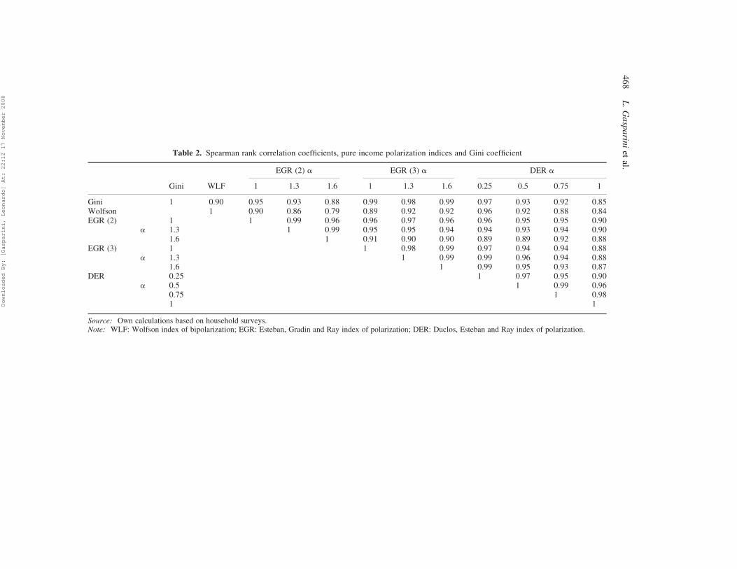
Table 2. Spearman rank correlation coefficients, pure income polarization indices and Gini coefficient
EGR (2) a EGR (3) a DER a
Gini WLF 1 1.3 1.6 1 1.3 1.6 0.25 0.5 0.75 1
Gini 1 0.90 0.95 0.93 0.88 0.99 0.98 0.99 0.97 0.93 0.92 0.85Wolfson 1 0.90 0.86 0.79 0.89 0.92 0.92 0.96 0.92 0.88 0.84EGR (2) 1 1 0.99 0.96 0.96 0.97 0.96 0.96 0.95 0.95 0.90
a 1.3 1 0.99 0.95 0.95 0.94 0.94 0.93 0.94 0.901.6 1 0.91 0.90 0.90 0.89 0.89 0.92 0.88
EGR (3) 1 1 0.98 0.99 0.97 0.94 0.94 0.88a 1.3 1 0.99 0.99 0.96 0.94 0.88
1.6 1 0.99 0.95 0.93 0.87DER 0.25 1 0.97 0.95 0.90
a 0.5 1 0.99 0.960.75 1 0.981 1
Source: Own calculations based on household surveys.Note: WLF: Wolfson index of bipolarization; EGR: Esteban, Gradin and Ray index of polarization; DER: Duclos, Esteban and Ray index of polarization.
46
8L
.G
asp
arin
iet
al.
Downloaded By: [Gasparini, Leonardo] At: 22:12 17 November 2008

economic performances have been substantially different, including changes in
income polarization. The heterogeneity of results provides a useful instrument to
identify specific policies and scenarios under which some countries have
managed to grow and/or become more equitable.
(ii) On average, small increase in polarization and inequality. As mentioned
above, more than half of the countries experienced increases in their levels of
polarization. However, changes in most countries have been rather small. On
average, polarization and inequality increased mildly in the region over the
period 1989–2004. Table 4 reports an increase of around 2.5% in the
polarization indicators. The average increase in the Gini was about the same.
(iii) Larger increase in polarization and inequality in South America in the 1990s.
The increase in the LAC average is driven by changes in South America
(Table 4). In most Central American countries changes have been almost
negligible. By contrast, in most (but not all) South American countries
inequality and polarization went up significantly. The increase seems to have
been particularly relevant in the early and mid-1990s, a period of relatively fast
growth and structural reforms. The pattern described fits the cases of Argentina,
Bolivia, Colombia, Paraguay, Peru, Uruguay and Venezuela, and probably
Ecuador. This process may be closely linked to the generation of social tension
as well as the existence of social unrest.
(iv) Convergence. Changes have implied some sort of convergence across LAC
countries: polarization and inequality have especially increased in the group
of less polarized/unequal countries: Argentina, Costa Rica, Uruguay and
Venezuela. The coefficient of variation of the polarization indicators and the
Gini coefficient have declined over time (see last row in Table 4).
3.4 What is the Difference Between Inequality and Polarization in Practice?
As explained in previous sections, income polarization and inequality are different although
related dimensions of the income distribution. The correlation between these two dimensions
is positive and statistically significant. Figure 5 displays the Gini coefficient and the
DER income polarization index for different a parameters. As a goes up, the weight of
Figure 4. Pure income polarization, DER index (a ¼ 0.5) for the household per capita incomedistribution. Urban and rural areas. Last survey available for each country. Source: Own calculations
based on household surveys. See Table 1.
Income Polarization in Latin America 469
Downloaded By: [Gasparini, Leonardo] At: 22:12 17 November 2008

Table 3. Pure income polarization, household per capita income, national statistics
EGR (2) a EGR (3) a DER a
Wolfson 1 1.3 1.6 1 1.3 1.6 0.25 0.5 0.75 1
Argentina15 cities
1992 0.410 0.204 0.150 0.107 0.730 0.494 0.339 0.334 0.284 0.269 0.2891998 0.485 0.228 0.168 0.121 0.803 0.545 0.373 0.355 0.294 0.270 0.272
28 cities1998 0.488 0.230 0.170 0.122 0.808 0.548 0.376 0.359 0.300 0.274 0.2772004 0.500 0.233 0.172 0.123 0.828 0.560 0.384 0.363 0.298 0.268 0.261
BoliviaUrban
1993 0.477 0.242 0.183 0.137 0.843 0.568 0.387 0.367 0.303 0.272 0.2591997 0.497 0.251 0.190 0.142 0.861 0.580 0.395 0.372 0.309 0.278 0.2652002 0.485 0.255 0.195 0.149 0.886 0.590 0.406 0.376 0.311 0.282 0.268
National1997 0.552 0.271 0.205 0.155 0.945 0.635 0.432 0.403 0.331 0.297 0.2862002 0.578 0.277 0.209 0.157 0.982 0.653 0.450 0.413 0.342 0.314 0.313
Brazil1990 0.648 0.302 0.233 0.181 0.998 0.666 0.460 0.425 0.363 0.344 0.3541998 0.607 0.292 0.226 0.175 0.977 0.651 0.449 0.414 0.356 0.350 0.3952003 0.569 0.279 0.214 0.164 0.949 0.639 0.436 0.402 0.344 0.346 0.399
Chile1990 0.501 0.267 0.206 0.160 0.908 0.604 0.415 0.385 0.319 0.289 0.2751998 0.518 0.270 0.209 0.161 0.912 0.607 0.418 0.384 0.318 0.289 0.2762003 0.476 0.258 0.199 0.153 0.888 0.590 0.406 0.376 0.312 0.283 0.269
ColombiaENH-Urban
1992 0.456 0.238 0.181 0.137 0.822 0.555 0.379 0.367 0.310 0.289 0.2992000 0.546 0.276 0.212 0.163 0.933 0.628 0.427 0.409 0.343 0.320 0.341
ECH-Urban2000 0.492 0.263 0.203 0.157 0.911 0.605 0.415 0.381 0.323 0.307 0.3252004 0.518 0.263 0.201 0.153 0.905 0.609 0.415 0.396 0.321 0.299 0.316
47
0L
.G
asp
arin
iet
al.
Downloaded By: [Gasparini, Leonardo] At: 22:12 17 November 2008

Costa Rica1992 0.406 0.195 0.140 0.097 0.715 0.485 0.333 0.326 0.262 0.223 0.1991997 0.412 0.199 0.144 0.100 0.725 0.493 0.338 0.324 0.260 0.221 0.1952003 0.464 0.223 0.164 0.118 0.794 0.538 0.368 0.345 0.278 0.241 0.219
Dominican Rep.2000 0.494 0.240 0.179 0.132 0.853 0.575 0.393 0.365 0.297 0.262 0.2432004 0.464 0.238 0.179 0.133 0.841 0.567 0.386 0.360 0.295 0.263 0.246
Ecuador1994 0.468 0.243 0.183 0.137 0.873 0.587 0.399 0.377 0.305 0.267 0.2481998 0.497 0.253 0.191 0.144 0.905 0.603 0.414 0.379 0.310 0.275 0.2582003 0.464 0.233 0.173 0.126 0.839 0.566 0.386 0.361 0.293 0.258 0.242
El Salvador1991 0.481 0.237 0.176 0.129 0.853 0.575 0.392 0.367 0.297 0.260 0.2402000 0.491 0.234 0.172 0.124 0.844 0.567 0.388 0.369 0.295 0.252 0.2272003 0.472 0.224 0.164 0.116 0.822 0.556 0.380 0.358 0.286 0.244 0.218
Guatemala2000 0.480 0.255 0.194 0.147 0.890 0.592 0.407 0.377 0.309 0.276 0.259
Haiti2001 0.558 0.285 0.221 0.171 0.973 0.646 0.443 0.406 0.334 0.300 0.283
HondurasOnly labor incomes
1992 0.522 0.247 0.185 0.136 0.873 0.590 0.402 0.372 0.304 0.270 0.2511997 0.503 0.249 0.187 0.139 0.890 0.600 0.408 0.379 0.310 0.275 0.257
All incomes1997 0.476 0.239 0.178 0.131 0.852 0.574 0.391 0.369 0.300 0.263 0.2412003 0.515 0.258 0.196 0.147 0.883 0.596 0.406 0.383 0.315 0.281 0.263
Jamaica1990 0.639 0.257 0.189 0.135 0.924 0.624 0.434 0.397 0.311 0.260 0.2261999 0.626 0.269 0.200 0.146 0.961 0.650 0.444 0.408 0.334 0.308 0.3172002 0.610 0.275 0.205 0.150 0.974 0.658 0.449 0.419 0.345 0.316 0.318
Mexico1992 0.478 0.255 0.195 0.149 0.894 0.600 0.407 0.375 0.308 0.276 0.2641996 0.474 0.241 0.181 0.135 0.856 0.577 0.393 0.364 0.297 0.264 0.248
Inco
me
Po
lariza
tion
inL
atin
Am
erica4
71
Downloaded By: [Gasparini, Leonardo] At: 22:12 17 November 2008

Table 3. Continued
EGR (2) a EGR (3) a DER a
Wolfson 1 1.3 1.6 1 1.3 1.6 0.25 0.5 0.75 1
2002 0.467 0.232 0.173 0.126 0.834 0.563 0.384 0.362 0.290 0.256 0.239Nicaragua
1993 0.548 0.261 0.195 0.144 0.919 0.620 0.422 0.391 0.318 0.281 0.2611998 0.475 0.244 0.183 0.136 0.876 0.584 0.401 0.379 0.308 0.271 0.2512001 0.478 0.249 0.188 0.142 0.886 0.589 0.404 0.375 0.310 0.279 0.263
Panama1995 0.545 0.257 0.192 0.141 0.900 0.609 0.416 0.385 0.306 0.262 0.2332003 0.572 0.265 0.200 0.149 0.922 0.623 0.426 0.393 0.321 0.285 0.269
Paraguay1997 0.557 0.256 0.190 0.138 0.920 0.621 0.425 0.395 0.319 0.281 0.2612002 0.557 0.259 0.193 0.141 0.927 0.625 0.426 0.392 0.318 0.281 0.262
Peru1997 0.514 0.243 0.180 0.131 0.871 0.589 0.402 0.378 0.306 0.267 0.2432002 0.502 0.247 0.185 0.137 0.885 0.590 0.407 0.382 0.312 0.274 0.251
Suriname1999 0.493 0.253 0.191 0.143 0.849 0.573 0.390 0.370 0.291 0.244 0.212
Uruguay1989 0.366 0.181 0.130 0.089 0.680 0.459 0.313 0.311 0.252 0.217 0.1931998 0.401 0.194 0.140 0.097 0.709 0.485 0.331 0.320 0.257 0.218 0.1912003 0.418 0.203 0.148 0.105 0.728 0.495 0.340 0.325 0.265 0.230 0.207
Venezuela1989 0.376 0.184 0.131 0.090 0.683 0.463 0.316 0.318 0.265 0.243 0.2461998 0.433 0.209 0.152 0.107 0.762 0.517 0.355 0.338 0.272 0.233 0.2102000 0.408 0.194 0.140 0.097 0.709 0.481 0.331 0.320 0.259 0.222 0.1992003 0.430 0.205 0.149 0.104 0.745 0.506 0.347 0.332 0.267 0.229 0.207
Source: Own estimates based on household surveys.Note: Wolfson: Wolfson index of bipolarization; EGR: Esteban, Gradin and Ray index of polarization; DER: Duclos, Esteban and Ray index of polarization.
47
2L
.G
asp
arin
iet
al.
Downloaded By: [Gasparini, Leonardo] At: 22:12 17 November 2008
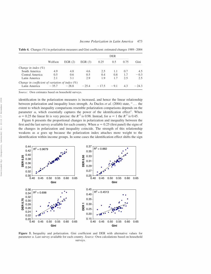
identification in the polarization measures is increased, and hence the linear relationship
between polarization and inequality loses strength. As Duclos et al. (2004) state, “ . . . the
extent to which inequality comparisons resemble polarization comparisons depends on the
parameter a, which essentially captures the power of the identification effect”. When
a ¼ 0.25 the linear fit is very precise: the R 2 is 0.98. Instead, for a ¼ 1 the R 2 is 0.45.
Figure 6 presents the proportional changes in polarization and inequality between the
first and the last survey available for each country. When a ¼ 0.25 (first panel) the signs of
the changes in polarization and inequality coincide. The strength of this relationship
weakens as a goes up because the polarization index attaches more weight to the
identification within income groups. In some cases the identification effect shifts the sign
Figure 5. Inequality and polarization. Gini coefficient and DER with alternative values forparameter a. Last survey available for each country. Source: Own calculations based on household
surveys.
Table 4. Changes (%) in polarization measures and Gini coefficient: estimated changes 1989–2004
DER
Wolfson EGR (2) EGR (3) 0.25 0.5 0.75 Gini
Change in index (%)South America 4.9 4.8 4.6 2.5 1.1 0.7 4.5Central America 0.5 0.6 0.5 0.4 0.8 1.7 20.3Latin America 2.1 3.1 2.9 1.9 1.7 2.5 2.5
Change in coefficient of variation of index (%)Latin America 235.7 228.8 225.4 217.5 29.1 4.3 224.3
Source: Own estimates based on household surveys.
Income Polarization in Latin America 473
Downloaded By: [Gasparini, Leonardo] At: 22:12 17 November 2008

of the overall polarization change. For instance, Brazil exhibits a decrease in polarization
for most indicators in the period 1990–2003, mainly because the decline in alienation
outweighs the increase in identification over the period. However, for a large a,
polarization stays roughly unchanged.
3.5 Who Contributes More to Income Polarization?
The DER polarization measure is the sum of all individual antagonisms in the society. It is
interesting to know how the different income strata contribute to overall polarization.
In order to accomplish this task, the population is partitioned into 20 income vintiles so the
sum of the antagonism of each vintile is the total DER measure.
Figure 7 indicates that the poorer vintiles contribute the most to total antagonism
because of their high identification. The lower the parameter a, the larger the contribution
to total polarization. The contribution of the richest vintiles is smaller due to their
relatively low identification, even though they have a more intense alienation. In other
words, although the richest vintiles are relatively farther away in the income dimension,
they are relatively more heterogeneous and thus less identified with their vicinity.
Given a level of total polarization, a homogeneous distribution of antagonism over
the population may lead to lower tension. By contrast, if the lowest vintiles are highly
polarized, then the high-level antagonism of this population potentially creates more
tension and would disrupt social cohesion. That seems to be the situation in most LAC
countries: on average, the first eight vintiles exceed their theoretical participation of 5% by
more than 1 percentage point.
3.6 A Decomposition
The DER polarization measure could be decomposed into three multiplicative
components: mean alienation (equal to the Gini coefficient), mean identification, and
Figure 6. Changes in inequality and polarization. Gini coefficient and DER with alternative valuesfor parameter a. Source: Own calculations based on household surveys.
474 L. Gasparini et al.
Downloaded By: [Gasparini, Leonardo] At: 22:12 17 November 2008

the rescaled correlation between individual alienation and identification.10 This
decomposition allows us to explore how these components interact in each income
distribution to determine total polarization.11 Table 5 considers the case of a ¼ 0.5. Brazil
has a lower level of average alienation (Gini coefficient) than Jamaica or Haiti, but the
Table 5. DER decomposition: alienation (Gini), identification and correlation effects, DER index(a ¼ 0.5)
Effects
Year Alienation Identification Correlation DER
Uruguay 2003 0.449 0.730 0.808 0.265Venezuela 2003 0.462 0.709 0.814 0.267Costa Rica 2003 0.490 0.716 0.794 0.278El Salvador 2003 0.509 0.703 0.797 0.286Suriname 1999 0.528 0.702 0.785 0.291Mexico 2002 0.514 0.729 0.780 0.292Ecuador 2003 0.517 0.737 0.768 0.293Dominican Rep 2004 0.514 0.755 0.760 0.295Argentina 2004 0.507 0.733 0.802 0.298Guatemala 2000 0.545 0.761 0.746 0.309Nicaragua 2001 0.543 0.770 0.741 0.310Peru 2002 0.543 0.745 0.770 0.312Chile 2003 0.540 0.783 0.738 0.312Honduras 2003 0.542 0.757 0.769 0.315Paraguay 2002 0.571 0.729 0.764 0.318Panama 2003 0.561 0.736 0.776 0.321Colombia 2004 0.551 0.772 0.774 0.329Haiti 2001 0.592 0.762 0.741 0.334Bolivia 2002 0.601 0.749 0.760 0.342Jamaica 2002 0.599 0.732 0.788 0.345Brazil 2003 0.576 0.799 0.763 0.351
Source: Own calculations based on household surveys.
Figure 7. Decomposition of the DER index: participation in DER by vintiles. Mean values across LACcountries. Last survey available for each country. Source: Own calculations based on household surveys.
Income Polarization in Latin America 475
Downloaded By: [Gasparini, Leonardo] At: 22:12 17 November 2008

average identification and the correlation counterbalance the first effect. Consider now two
countries with the same level of average alienation, such as Mexico and Dominican
Republic. They end up with different levels of polarization because of a higher level of
identification in the latter country.
4. Income Distribution, Institutions and Conflicts
It has long been argued that the income distribution of a country is associated with
its institutional development and its degree of social cohesion and unrest. An economy
in which income is more equally distributed is probably characterized by better and more
stable institutions, fewer conflicts and a stronger sense of social cohesion. However,
although intuitive, the links are theoretically ambiguous and have not been well established
by the empirical literature. The difficulties are enormous: (i) there are no obvious empirical
counterparts for concepts such as institutions, social cohesion and conflicts; (ii) the theory
stresses that causality may go in all directions; (iii) it is not clear which dimension of the
income distribution (inequality, polarization, poverty, mobility) is the most relevant; and
(iv) the data at hand are insufficient to implement valid tests for causality.
Despite these empirical limitations, the topic is sufficiently important to have attracted
the attention of social scientists for decades. The academic community is continuously
searching for new datasets and ideas that contribute to the understanding of the links
between income distribution, institutions and conflicts. The issue is particularly relevant
for Latin America and the Caribbean. This region has arguably the highest levels of
income disparities in the world, and it is also one of the regions with weakest institutions,
and highest levels of unrest and violence. Moreover, the evidence suggests increasing
income disparities in several LAC countries over the last two decades, raising questions
about the implications for socio-political instability.
In this section we analyze the interactions between several measures of institutions and
conflict with three different dimensions of the income distribution: polarization, inequality
and poverty. As suggested above, causality issues are extremely difficult to solve, so in this
paper we just show the structure of correlations among variables, and try to lay down
consistent interpretations of the results based on theoretical considerations.
4.1 Institutions
The literature linking income distribution with institutions has been growing at a fast pace.
Ritzen et al. (2006) put forward the hypothesis that social cohesion—in their paper
measured by income inequality, share of middle class and ethnic fractionalization—
determines institutional quality, which in turn is a key determinant for economic growth.
In a similar vein, Keefer & Knack (2002) conjectured that social polarization—measured
as income inequality, land inequality and ethnic fragmentation—affects growth through
the institutional channel. Glaeser (2005) found that a balanced income distribution is
highly correlated with high-quality institutions, but is very careful not to speak of causality
given the identification problems noted above. Chong & Gradstein (2004) found
supporting evidence for the idea of bidirectional causality making use of Generalized
Method of Moments (GMM) techniques and Vector Auto Regression (VAR). They
concluded that the link that goes from income inequality to institutions is stronger than the
one that goes the other way. Cervellati & Sunde (2005) also support the idea of
476 L. Gasparini et al.
Downloaded By: [Gasparini, Leonardo] At: 22:12 17 November 2008

bidirectional causality between institutions and inequality. Engerman & Sokoloff (2002,
2005) argue that initial factor endowments, such as the distribution of wealth, human
capital and political power, play a key role in accounting for the dissimilar degree of
institutional development among former colonies. Boix (2003) also argues that higher
income inequality induces a lower probability of democratization.
In short, the literature points out that the income distribution may interact with the
broad-based institutions of a country. Empirical measures for these institutions typically
combine information on formal constraints with measures of the actual functioning of
certain institutions and rules. In the Appendix we provide details on the set of indices used
in this paper, which includes measures of democracy, government effectiveness, security
of property rights, political constraints, rule of law, and voice and accountability.
Naturally, these indicators are just proxies of very complex phenomena, and then subject
to all sorts of measurement errors. However, in the absence of better data and to
complement the theoretical analysis, the empirical literature has used these indicators
extensively in search of regularities and associations with other variables.
In the following, we explore the correlations between measures of institutions and
indicators of three dimensions of the income distribution: polarization, inequality and
absolute poverty. We measure inequality with the traditional Gini coefficient, polarization
with the DER for a ¼ 0.5, and absolute poverty with the headcount ratio with a poverty
line of US$2 Purchasing Power Parity (PPP) a day.12 The first column in each panel of
Table 6 shows correlations for the pooled dataset, and in the following two columns the
Table 6. Correlations between indicators of income distribution and institutions
Correlations
pooled period 1 period 2 controlling for GDP pc
Rule of Law 20.5457* 20.6011* 20.4523* 20.4176*Voice and Accountability 20.4180* 20.4317* 20.3966* 20.2802*Legal structure 20.2688 20.161 20.3336 20.106Gov’t Effectiveness 20.4704* 20.5236* 20.3946 20.2941*Democracy 20.2058 20.2019 20.2291 20.1648Political constraints 20.0393 0.0522 20.114 20.089
Inequality (Gini)
Rule of Law 20.6272* 20.6467* 20.5831* 20.4289*Voice and Accountability 20.5136* 20.5032* 20.5267* 20.3303*Legal structure 20.3454* 20.2393 20.4468* 20.1128Gov’t Effectiveness 20.6044* 20.6702* 20.5218* 20.3531*Democracy 20.2772 20.2623 20.3264 20.2358Political constraints 20.1476 20.1215 20.1385 0.025
Poverty (headcount ratio)
Rule of Law 20.6802* 20.7298* 20.7071* 20.3916*Voice and Accountability 20.5230* 20.4888* 20.5679* 20.2532*Legal structure 20.4992* 20.5127* 20.5562* 20.1814Gov’t Effectiveness 20.6858* 20.7065* 20.6967* 20.2882Democracy 20.3869* 20.1622 20.6911* 20.4336*Political constraints 20.3850* 20.4429* 20.319 20.2144
*Significant at 10%.Note: period 1 ¼ 1989–98, period 2 ¼ 1999–2004.
Income Polarization in Latin America 477
Downloaded By: [Gasparini, Leonardo] At: 22:12 17 November 2008
sample is divided into two periods: 1989–98 (a period of economic growth) and 1999–
2004 (recession and start of the recovery). The last column shows correlations when
controlling for per capita GDP.
There is a close link between the income distribution and the institutional strength of a
country. The correlations in Table 6 suggest that more polarized/unequal/poor countries
are on average also those with weaker institutions. The correlations seem particularly
strong with the Rule of Law index, the Voice and Accountability indicator, and the
Government Effectiveness index. Poverty is also significantly negatively correlated to the
Democracy index. Most of the correlations remain significant when controlling for per
capita GDP, although the values are substantially reduced. The links become weaker or
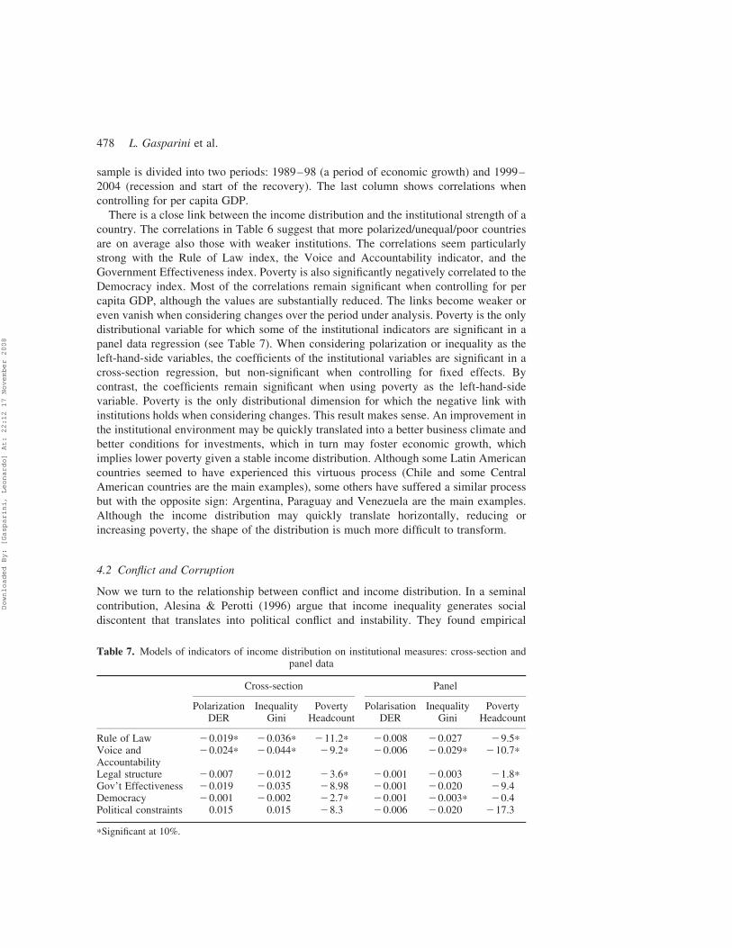
even vanish when considering changes over the period under analysis. Poverty is the only
distributional variable for which some of the institutional indicators are significant in a
panel data regression (see Table 7). When considering polarization or inequality as the
left-hand-side variables, the coefficients of the institutional variables are significant in a
cross-section regression, but non-significant when controlling for fixed effects. By
contrast, the coefficients remain significant when using poverty as the left-hand-side
variable. Poverty is the only distributional dimension for which the negative link with
institutions holds when considering changes. This result makes sense. An improvement in
the institutional environment may be quickly translated into a better business climate and
better conditions for investments, which in turn may foster economic growth, which
implies lower poverty given a stable income distribution. Although some Latin American
countries seemed to have experienced this virtuous process (Chile and some Central
American countries are the main examples), some others have suffered a similar process
but with the opposite sign: Argentina, Paraguay and Venezuela are the main examples.
Although the income distribution may quickly translate horizontally, reducing or
increasing poverty, the shape of the distribution is much more difficult to transform.
4.2 Conflict and Corruption
Now we turn to the relationship between conflict and income distribution. In a seminal
contribution, Alesina & Perotti (1996) argue that income inequality generates social
discontent that translates into political conflict and instability. They found empirical
Table 7. Models of indicators of income distribution on institutional measures: cross-section andpanel data
Cross-section Panel
PolarizationDER
InequalityGini
PovertyHeadcount
PolarisationDER
InequalityGini
PovertyHeadcount
Rule of Law 20.019* 20.036* 211.2* 20.008 20.027 29.5*Voice andAccountability
20.024* 20.044* 29.2* 20.006 20.029* 210.7*
Legal structure 20.007 20.012 23.6* 20.001 20.003 21.8*Gov’t Effectiveness 20.019 20.035 28.98 20.001 20.020 29.4Democracy 20.001 20.002 22.7* 20.001 20.003* 20.4Political constraints 0.015 0.015 28.3 20.006 20.020 217.3
*Significant at 10%.
478 L. Gasparini et al.
Downloaded By: [Gasparini, Leonardo] At: 22:12 17 November 2008

evidence validating the hypothesis in a sample of 70 countries for the period 1960–85.
Sachs (1990) studied how high income inequality in Latin America stimulates social
disorder and political conflict. The literature linking corruption and income distribution is
also vast and growing. The theoretical underpinnings for this link are drawn from the ideas
of Krueger (1974), who asserts that corruption distorts institutions of governance, and
through the institutional channel affects the income distribution. More recently, Li et al.
(2000), Sanjeev et al. (2002) and Dincer & Gunalp (2005) found significant correlations
between corruption and income inequality.
As discussed above, our dataset does not allow us to disentangle causal relationships.
However, and following most of the literature, in the discussions of this section we
implicitly tend to view conflicts as caused, among other factors, by different dimensions of
the income distribution. We also briefly examine the potential relationship between the
income distribution and corruption. In order to capture the level of conflict in the society
we use the Political Stability and Absence of Conflict index of Kaufmann et al. (2005), and
to measure corruption we use the Control of Corruption index constructed by the same
authors (see the Appendix for details).
The correlations in Table 8 suggest that more polarized/unequal/poor countries are on
average also those with higher levels of conflict. The correlations with the conflict index
remain significant when controlling for per capita GDP. In fact, the values are almost
unchanged when including controls. The correlations with the measures of control of
corruption have the expected sign (negative), although the relationships do not seem
strong, in particular when we control for other variables.
Table 9 shows the results of panel regressions where we control for fixed effects. Changes in
polarization, inequality and poverty seem to be related to changes in conflict. This piece of
Table 8. Correlations between indicators of income distribution and conflict and corruption
Correlations
pooled period 1 period 2 controling for GDP pc
Polarization (PER 0.5)Conflict 20.4486* 20.4859* 20.4120* 20.4346*Control of Corruption 20.1799 20.0687 20.2768 20.0465
Inequality (Gini)Conflict 20.4522* 20.4417* 20.4710* 20.4097*Control of Corruption 20.2977* 20.1892 20.4273* 20.0757
Poverty (headcount ratio)Conflict 20.5123* 20.5313* 20.5023* 20.2747*Control of Corruption 20.4766* 20.4191* 20.5351* 20.1593
*Significant at 10%.
Table 9. Models of indicators of income distribution on conflict and corruption measures: panel data
Conflict Control of Corruption
Polarization (DER) 214.498* 5.886Inequality (Gini) 28.757* 0.920Poverty (Headcount) 20.015* 20.005
*Significant at 10%.
Income Polarization in Latin America 479
Downloaded By: [Gasparini, Leonardo] At: 22:12 17 November 2008
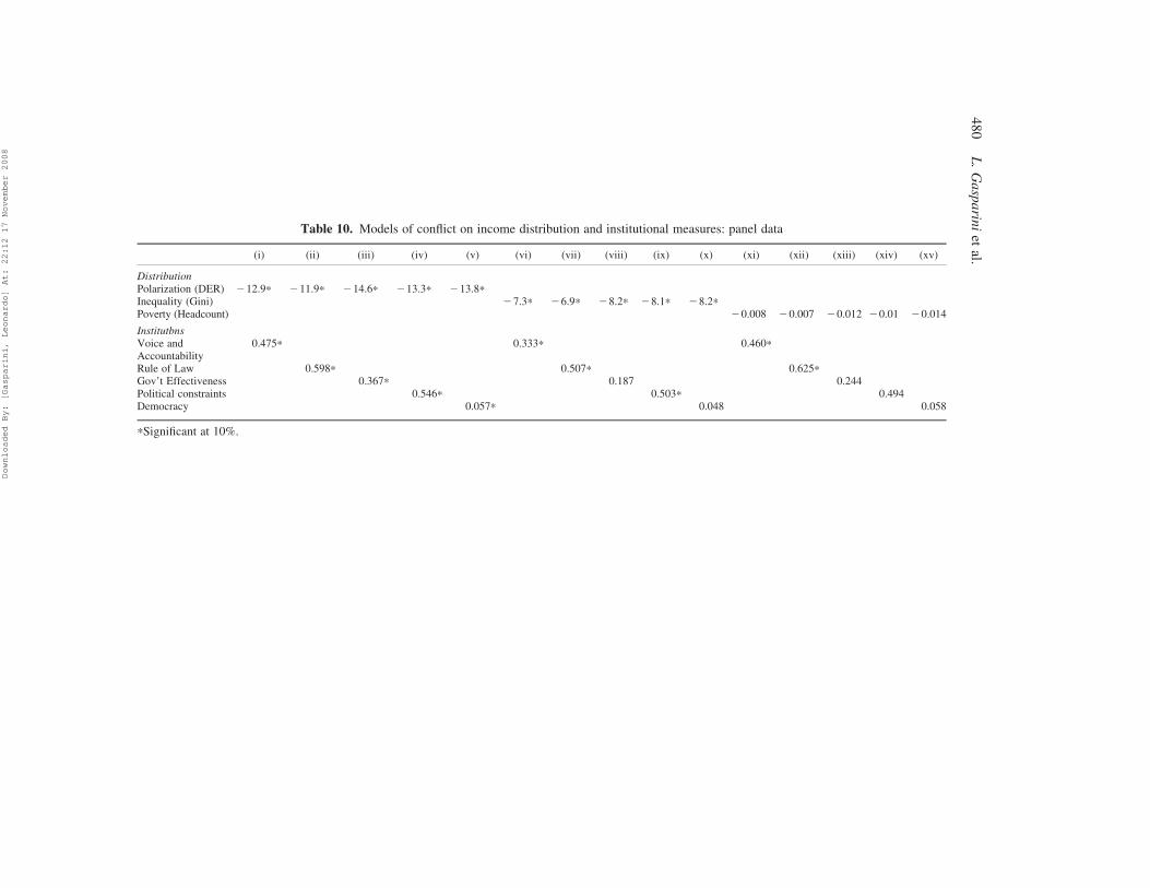
Table 10. Models of conflict on income distribution and institutional measures: panel data
(i) (ii) (iii) (iv) (v) (vi) (vii) (viii) (ix) (x) (xi) (xii) (xiii) (xiv) (xv)
DistributionPolarization (DER) 212.9* 211.9* 214.6* 213.3* 213.8*Inequality (Gini) 27.3* 26.9* 28.2* 28.1* 28.2*Poverty (Headcount) 20.008 20.007 20.012 20.01 20.014
InstitutbnsVoice andAccountability
0.475* 0.333* 0.460*
Rule of Law 0.598* 0.507* 0.625*Gov’t Effectiveness 0.367* 0.187 0.244Political constraints 0.546* 0.503* 0.494Democracy 0.057* 0.048 0.058
*Significant at 10%.
48
0L
.G
asp
arin
iet
al.
Downloaded By: [Gasparini, Leonardo] At: 22:12 17 November 2008

evidence is consistent with the idea that increasing levels of polarization, inequality and
poverty generate a hostile atmosphere within society that could imply higher levels of social
conflict and political instability. The relationship with corruption, by contrast, is not clear.
In what follows we include a set of institutional controls to the analysis. It has long been
argued that institutions are key features for understanding social conflicts. The regression
results for the conflict index when institutions are included in the analysis are shown in
Table 10. On the right-hand side we include income distribution measures, along with
institutional indicators and various other controls (e.g. GDP per capita). The results
suggest that both polarization and inequality are closely related to situations of conflict.
The measures of these distributional dimensions are always significant when controlling
for different institutional variables. That is not the case with the poverty headcount ratio:
coefficients have the expected signs but seem to be non-significant.
Some interesting results emerge from the analysis of this section. First, the results of the
regressions suggest that both income distribution and institutions do matter for social conflict
and instability. Second, only distributional measures that capture income disparities seem to
be particularly relevant to understanding conflicts. Finally, the LAC data do not support the
idea that polarization, not inequality, is the main distributional characteristic associated with
social instability. The high correlation between polarization and inequality found in the data
implies that most results apply to both income distribution dimensions. In particular,
polarization does not turn out to be a better predictor of conflict than inequality.
5. Concluding Comments
It has long been argued that Latin American and Caribbean countries are among the most
unequal economies in the world. From the evidence shown in this study the region is also
characterized by a high degree of polarization, i.e. a situation in which homogeneous
groups antagonize each other. Moreover, there are some worrying signs of increasing or at
least non-decreasing economic polarization in the region over the last 15 years, which may
reinforce the latent sources of social tension.
Experiences have been heterogeneous across LAC countries. Distributional changes
have been large in some countries, and negligible in others. On average, income polarization
increased in most of South America, and stayed roughly unchanged in Central America.
The paper suggests that institutions and conflict interact in different ways with the
various characteristics of the income distribution. There is some evidence that in the LAC
context institutional development has been associated with lower absolute poverty, but not
significantly with lower polarization and inequality. Instead, conflicts seem to be more
related to polarization and inequality than to poverty.
Polarization and inequality measures are highly correlated in the data. At least in the
Latin American context and for the indicators used in this paper, income inequality seems
a good proxy for income polarization.
Notes
1 See IADB (1998), Morley (2000), Ganuza et al. (2001), Bourguignon & Morrison (2002) and
Gasparini (2003) for evidence on inequality in LAC.2 See Esteban & Ray (1994) and Foster & Wolfson (1992).3 Gasparini (2003) includes evidence on bipolarization for a set of Latin American countries.
Income Polarization in Latin America 481
Downloaded By: [Gasparini, Leonardo] At: 22:12 17 November 2008

4 The literature on polarization by characteristics has recently been increasing rapidly. Collier &
Hoeffler (2001) measure polarization in an empirical analysis of civil war, Reynal-Querol (2001)
studies polarization by religion groups and its relationship with the probability of a conflict in sub-
Saharan countries, D’Ambrosio (2001) argues that the region of residence accounts for polarization in
the Italian distribution of personal income, Gradın (2000) finds that education and socio-economic
condition are the key variables to explain polarization in the Spanish distribution of income and Zhang
& Kanbur (2001) apply some polarization measures to regional disparities in China.5 See Duclos et al. (2004) for methodological details. The DER index ranges from zero (absence of
polarization) to one (full polarization).6 See the web site of the SEDLAC at www.cedlas.org for details.7 See the Guide in the web site of the SEDLAC for methodological details.8 More information on changes in polarization by country can be found in Gasparini et al. (2006).9 Changes can be studied for a sample of 16 countries. There are not enough comparable surveys to
analyze patterns over the 1990s and 2000s in Dominican Republic, Ecuador, Guatemala, Haiti and
Suriname.10 For further details see Duclos et al. (2004).11 Of course, it is impossible to move these components independently, because they are all interrelated
dimensions of the same distribution.12 See Gasparini et al. (2007) for a discussion on poverty measurement and trends in LAC using a similar
database as in this paper.
References
Alesina, A. & Perotti, R. (1996) Income distribution, political instability, and investment, European Economic
Review, 40, pp. 1203–1228.
Boix, C. (2003) Democracy and Redistribution (Cambridge: Cambridge University Press).
Bourguignon, F. & Morrison, C. (2002) Inequality among world citizens: 1820–1992, American Economic
Review, 92, pp. 727–743.
Cervellati, P. & Sunde, U. (2005) Hobbes to Rousseau: inequality, institutions, and development, IZA Discussion
Paper No. 1450.
Chong, A. & Gradstein, M. (2004) Inequality and Institutions, CEPR Discussion Paper 4739.
Collier, P. & Hoeffler, A. (2001) Greed and Grievance in Civil War (Washington, DC: The World Bank).
D’Ambrosio, C. (2001) Household characteristics and the distribution of income in Italy: an application of
social distance measures, Review of Income and Wealth, 47(1), pp. 43–64.
Dincer, C. & Gunalp, B. (2005) Corruption, income inequality, and growth: evidence from U.S, states,
unpublished manuscript, Massey University, Auckland.
Duclos, J., Esteban, J. & Ray, D. (2004) Polarization: concepts, measurements, estimation, Econometrica, 72,
pp. 1737–1772.
Engerman, S. & Sokoloff, K. (2005) Colonialism, Inequality, and Long-run Paths of Development, NBER
Working Paper No. W11057.
Engerman, S. & Sokoloff, K. (2002) Factor Endowments, Inequality, and Paths of Development Among New
World Economies, NBER Working Paper No. 9259.
Esteban, J., Gradın, C. & Ray, D. (2007) Extensions of the measure of polarization, with an application to the
income distribution of five OECD countries, Journal of Economic Inequality, 5, pp. 1–19.
Esteban, J. & Ray, D. (1994) On the measurement of polarization, Econometrica, 62, pp. 819–852.
Foster, J. & Wolfson, M. (1992) Polarization and the decline of the middle class: Canada and the US. unpublished
manuscript, Vanderbilt University.
Ganuza, E., Paes de Barros, R., Taylor, L. & Vos, R. (2001) Liberalizacion, desigualdad y pobreza: America
Latina y el Caribe en los 90, Eudeba, PNUD, CEPAL, Buenos Aires.
Gasparini, L. (2003) Different Lives: Inequality in Latin America and the Caribbean, Working Paper CEDLAS,
chapter 2, 2004 World Bank LAC Flagship Report, Washington DC.
Gasparini, L., Gutierrez, F. & Tornarolli, L. (2007) Growth and income poverty in Latin America and the
Caribbean: evidence from household surveys, Review of Income and Wealth, 53, pp. 209–245.
Gasparini, L., Horenstein, M. & Olivieri, S. (2006) Economic Polarisation in Latin America and the Caribbean:
What do Household Surveys Tell Us?, Working Paper No. 38, CEDLAS.
482 L. Gasparini et al.
Downloaded By: [Gasparini, Leonardo] At: 22:12 17 November 2008

Glaeser, E. (2005) Inequality, in: B. R. Weingast & D. Wittman (Eds) Oxford Handbook of Political Economy
(Oxford: Oxford University Press).
Gradın, C. (2000) Polarization by sub-populations in Spain, 1973–91, Review of Income and Wealth, 46(4),
457–474.
Gwartney, J. & Lawson, R. (2005) Economic Freedom of the World: 2005 Annual Report (Vancouver: The Fraser
Institute).
Henisz, W. (2002) The institutional environment for infrastructure investment, Industrial and Corporate Change,
11(2), 355–389.
IADB (1998) America Latina Frente a la Desigualdad (Washington, DC: Banco Interamericano de Desarrollo).
Kaufmann, D., Kraay, A. & Mastruzzi, M. (2005) Governance Matters IV: Governance Indicators for 1996–
2004, Draft, May 2005.
Keefer, P. & Knack, S. (2002) Polarization, politics and property rights: links between inequality and growth,
Public Choice, 111(1–2), pp. 127–154.
Krueger, A. (1974) The political economy of the rent-seeking society, American Economic Review, 64(3),
pp. 291–303.
Li, H., Xu, L. C. & Zou, H. (2000) Corruption, income distribution, and growth, Economics and Politics, 12(2),
pp. 155–182.
Morley, S. (2000) La distribucion del ingreso en America latina y el Caribe, CEPAL/Fondo de Cultura
Economica, Santiago.
Polity IV Project: Integrated Network for Societal Conflict Research (INSCR) Program Center for International
Development and Conflict Management (CIDCM) University of Maryland, College Park 20742
www.cidcm.umd.edu/inscr/polity q 2002.
Reynal-Querol, M. (2001) Ethnicity, Political System and Civil Wars, Mimeo, Institut d’Analisis Economic
(IAE) (Barcelona: CSIC).
Ritzen, J., Easterly, W. & Woolcock, M. (2006) Social cohesion, institutions, and growth, Economics and
Politics, 18(2), pp. 103–120.
Sachs, J. (1990) Social conflict and populist policies in Latin America, in: R. Brunetta & C. Dell’Aringa (Eds)
Labor Relations and Economic Performance (New York: NYU Press).
Sanjeev, G., Davoodi, H. & Alonso-Terme, R. (2002) Does corruption affect income inequality and poverty?,
Economics of Governance, 3(1), pp. 23–45.
Wolfson, M. (1994) When inequality diverges, American Economic Review, 84, pp. 353–358.
Zhang, X. & Kanbur, R. (2001) What difference do polarization measures make? An application to China,
Journal of Development Studies, 37, pp. 85–98.
Appendix
Broad-based Institutions Indices
Rule of Law index. This index is measured in units ranging from 22.5 to 2.5, with higher
values corresponding, in broad terms, to the respect of citizens and the state for the
institutions that govern their interactions. Source: Kaufmann et al. (2005).
Voice and accountability index. This index is a measure of the extent to which citizens of
a country are able to participate in the selection of governments. It includes a number of
indicators measuring various aspects of the political process, civil liberties and political
rights. The index is measured in units ranging from 22.5 to 2.5, with higher values
corresponding to a system where citizens have more voice and accountability. Source:
Kaufmann et al. (2005).
Legal structure and security of property rights index. This index is a measure of the
functioning of the legal system in a country. It is measured in units ranging from 0 to 10,
Income Polarization in Latin America 483
Downloaded By: [Gasparini, Leonardo] At: 22:12 17 November 2008

with higher values corresponding to a system with a better working of the legal system.
Source: Gwartney & Lawson (2005).
Government effectiveness index. This index is a measure of the quality of public service
provision, the quality of the bureaucracy, the competence of civil servants, the
independence of the civil service from political pressures, and the credibility of
government commitment to policies. It is measured in units ranging from 22.5 to 2.5,
with higher values corresponding to a more effective government. Source: Kaufmann et al.
(2005).
Democracy index. This index is a measure of the degree of institutionalized democracy.
The index is measured in units ranging from 210 to 10, with higher values corresponding
to a system with a more consolidated democracy. Source: Polity IV Project.
Political constraints index. This index estimates the feasibility of policy changes. The
index is measured in units ranging from 0 to 1, with higher values corresponding to a
system where policy changes are more feasible. Source: Henisz (2002).
Conflict and Corruption Indices
Political stability and absence of violence index. This index is measured in units ranging
from 22.5 to 2.5, with higher values corresponding to a system that is least likely to be
destabilized or overthrown, and where conflicts play no part in the society. Source:
Kaufmann et al. (2005).
Control of corruption index. This index is a measure of perceptions of corruption,
defined as the exercise of public power for private gain. It is measured in units ranging
from about 22.5 to 2.5, with higher values corresponding to less corruption. Source:
Kaufmann et al. (2005).
484 L. Gasparini et al.
Downloaded By: [Gasparini, Leonardo] At: 22:12 17 November 2008


