income polarisation - aaep.org.ar · this paper combines the results of two working papers:...
TRANSCRIPT

Income Polarisation:
An exploratory analysis for Latin America *
Leonardo Gasparini **
Matías Horenstein Ezequiel Molina Sergio Olivieri
CEDLAS ***
Universidad Nacional de La Plata
Abstract
This document presents a set of statistics that characterise the degree of income polarisation in Latin American and the Caribbean (LAC). The study is based on a dataset of household surveys from 21 LAC countries in the period 1989-2004. Latin America is characterised by a high level of income polarisation. On average, income polarisation has mildly increased in the region since the early 1990s. The paper suggests that institutions and conflict interact in different ways with the various characteristics of the income distribution. In particular, countries with high income polarisation and inequality are more likely to have high levels of conflict and corruption.
Keywords: polarisation, cohesion, inequality, Latin America, Caribbean, conflict
JEL codes: I3, D3, D6
* This document is part of a project on Social Cohesion in Latin America and the Caribbean carried out by CEDLAS and UNDP. This paper combines the results of two working papers: Gasparini, Horenstein and Olivieri (2006) and Gasparini and Molina (2006). The authors are very grateful to Enrique Ganuza, Stefano Petinatto, Patricio Meller, André Urani, Gerardo Munck and Ana Pacheco for valuable comments and suggestions. All the views expressed in the paper are the sole responsibility of the authors. ** E-mails: [email protected], [email protected], [email protected], and [email protected]. *** CEDLAS is the Center for Distributional, Labor and Social Studies at Universidad Nacional de La Plata (Argentina). www.depeco.econo.unlp.edu.ar/cedlas
1

1. Introduction
There is an increasing concern on issues of polarisation and social cohesion arising from the observation that some societies may be separating out into groups internally homogenous and increasingly different among them. That concern is particularly relevant in Latin America and the Caribbean (LAC), a region with traditionally very high levels of inequality, and increasing income disparities over the last two decades.1
This study documents the levels and trends of income polarisation in LAC by exploiting a large database of household surveys carried out in 21 countries in the period 1989-2004. The document shows evidence suggesting that Latin America is characterised by a high level of income polarisation, compared to other regions in the world. On average, income polarisation has mildly increased in the region since the early 1990s. The country experiences, however, have been heterogeneous. While income polarisation substantially increased in some countries, the income distributions of other LAC economies turned less polarised.
It is argued that when people have access to substantially different sets of opportunities, and enjoy (or suffer) very different living standards, social tensions are likely to emerge. An economically polarised country is more likely to be socially and politically unstable.2 In this paper we present a set of correlations between (i) measures of income polarisation and other dimensions of the income distribution, and (ii) measures of institutions, conflict and corruption. Although far from a causality analysis, the paper provides evidence on some interesting links that deserve further analysis.
The rest of the document is organised as follows. In section 2 we discuss the definition and measurement of income polarisation. Section 3 presents empirical evidence on income polarisation in LAC, and discusses the main patterns and trends. In Section 4 we carry out an exploratory analysis of the empirical links between indicators of polarisation, inequality and poverty, and measures of institutions, conflict and corruption. We include some concluding remarks in section 5.
2. Polarisation: concept and measurement
The concept of polarisation is directly linked to the sources of social tension. The notion has its roots in sociology and political science, with Karl Marx arguably being the first social scientist to study it. In Economics its formal analysis has its origins in the 1990s, in the works of Esteban and Ray (1991, 1994), Foster and Wolfson (1992) and Wolfson (1994). Following Esteban and Ray (1994) we rely on what might be called the alienation-identification framework. The intuition is simple: given a relevant characteristic such as religion, income, race or education, a population is polarised if there are few groups of important size in which their members share this attribute and feel some degree of identification with members of their own group, and at the same time, members of different groups feel alienated from each other. This three elements (size group, identification and alienation) produce antagonism among the population which may generate a hostile environment.
The concern for differences in economic variables across groups has always been in the Economics agenda. That concern fuelled a large literature on the measurement of inequality. The concept of inequality is closely linked to the principle of Dalton-Pigou: a transfer from an
1 See IADB (1998), Morley (2000), Ganuza et al. (2001), Bourguignon and Morrison (2003) and Gasparini (2004 a) for evidence on inequality in LAC. 2 Of course, the causality can go both directions: socioeconomic fragmentation can be the consequence of social and political instability.
2

individual with higher income to another individual with lower income generates a more equal distribution.
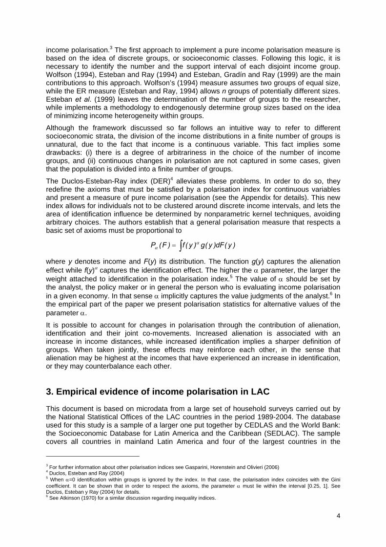
To understand the difference between polarisation and inequality, suppose a country with six persons labelled as A, B, C, D, E, F with incomes equal to $ 1, 2, 3, 4, 5 and 6, respectively. Assume now two transfers of one peso: the first one from C to A, and the second one from F to D. The two transfers are equalizing (from richer to poorer persons), so all inequality indices complying with the Dalton-Pigou criterion will fall, or at least not increase. The inequality analysis assesses the new situation as “better” than the initial one. Notice, however, that in this example the new income distribution has three persons with $2 (A, B and C), and three persons with $5 (D, E and F). The population in this country is divided into two clearly differentiated groups that are internally perfectly homogeneous. Although less unequal, this society has become more polarised. The notion of polarisation refers to homogeneous clusters that antagonize with each other. In the new situation of the example people may identify themselves as part of clearly defined groups which are significantly different from the rest. This polarisation may derive in greater social tension than in the initial distribution, and then in more social and political instability. In fact, the conjecture that motivates research on polarisation is that contrasts among densely homogeneous groups may cause social tension. Histograms of the income distribution Before and after an inequality-decreasing but polarisation-increasing transfer
Before transfers
0
1
2
3
1 2 3 4 5 6Income levels
After transfers
0
1
2
3
1 2 3 4 5 6Income levels
Less unequalMore polarised
The previous example is intended to illustrate a case where polarisation goes in opposite direction to inequality. But it is likely that in most cases the two concepts do not disagree. Suppose that from the initial distribution there is a transfer of $1 from B to E: the economy is now more unequal and more polarised. The analysis of polarisation should be viewed as complementary to that of inequality. Both polarisation and inequality are different although related dimensions of the same distribution. Two reasons led us to focus this paper on polarisation. First, polarisation is by far the distributional dimension less studied in the economic literature. While the inequality literature is large in Latin America, we are not aware of studies computing polarisation measures for a large set of countries in the region. Second, polarisation measures may potentially be more relevant than inequality measures to study issues of socio-political instability. We explore this point with LAC data.
Measurement
This paper restricts the analysis of polarisation to the income dimension. Income polarisation measures could be classified into two main sets: polarisation by characteristics and pure income polarization. Although both sets use income as the variable for alienation, they differ in the nature of identification. While the first uses a discrete variable to provide the relevant grouping of the population (e.g. race), the latter uses income. In this paper we focus on pure
3
income polarisation.3 The first approach to implement a pure income polarisation measure is based on the idea of discrete groups, or socioeconomic classes. Following this logic, it is necessary to identify the number and the support interval of each disjoint income group. Wolfson (1994), Esteban and Ray (1994) and Esteban, Gradín and Ray (1999) are the main contributions to this approach. Wolfson’s (1994) measure assumes two groups of equal size, while the ER measure (Esteban and Ray, 1994) allows n groups of potentially different sizes. Esteban et al. (1999) leaves the determination of the number of groups to the researcher, while implements a methodology to endogenously determine group sizes based on the idea of minimizing income heterogeneity within groups.
Although the framework discussed so far follows an intuitive way to refer to different socioeconomic strata, the division of the income distributions in a finite number of groups is unnatural, due to the fact that income is a continuous variable. This fact implies some drawbacks: (i) there is a degree of arbitrariness in the choice of the number of income groups, and (ii) continuous changes in polarisation are not captured in some cases, given that the population is divided into a finite number of groups.
The Duclos-Esteban-Ray index (DER)4 alleviates these problems. In order to do so, they redefine the axioms that must be satisfied by a polarisation index for continuous variables and present a measure of pure income polarisation (see the Appendix for details). This new index allows for individuals not to be clustered around discrete income intervals, and lets the area of identification influence be determined by nonparametric kernel techniques, avoiding arbitrary choices. The authors establish that a general polarisation measure that respects a basic set of axioms must be proportional to
∫= )y(dF)y(g)y(f)F(P αα
where y denotes income and F(y) its distribution. The function g(y) captures the alienation effect while f(y)α captures the identification effect. The higher the α parameter, the larger the weight attached to identification in the polarisation index.5 The value of α should be set by the analyst, the policy maker or in general the person who is evaluating income polarisation in a given economy. In that sense α implicitly captures the value judgments of the analyst.6 In the empirical part of the paper we present polarisation statistics for alternative values of the parameter α.
It is possible to account for changes in polarisation through the contribution of alienation, identification and their joint co-movements. Increased alienation is associated with an increase in income distances, while increased identification implies a sharper definition of groups. When taken jointly, these effects may reinforce each other, in the sense that alienation may be highest at the incomes that have experienced an increase in identification, or they may counterbalance each other.
3. Empirical evidence of income polarisation in LAC
This document is based on microdata from a large set of household surveys carried out by the National Statistical Offices of the LAC countries in the period 1989-2004. The database used for this study is a sample of a larger one put together by CEDLAS and the World Bank: the Socioeconomic Database for Latin America and the Caribbean (SEDLAC). The sample covers all countries in mainland Latin America and four of the largest countries in the
3 For further information about other polarisation indices see Gasparini, Horenstein and Olivieri (2006) 4 Duclos, Esteban and Ray (2004) 5 When α=0 identification within groups is ignored by the index. In that case, the polarisation index coincides with the Gini coefficient. It can be shown that in order to respect the axioms, the parameter α must lie within the interval [0.25, 1]. See Duclos, Esteban y Ray (2004) for details. 6 See Atkinson (1970) for a similar discussion regarding inequality indices.
4

Caribbean (Table 3.1). Most household surveys included in the sample are nationally representative. In each period the sample of countries represents more than 92% of LAC total population. Whenever possible we select three years in each country to characterize the two main periods in the last 15 years: the growth period of the early and mid 1990s when several structural reforms were implemented, and the stagnation and crisis period of the late 1990s and early 2000s. Unfortunately, there is not enough information to characterize the recent recovery of the LAC economies that started around 2003.
For comparability purposes we compute income using a common methodology across countries and years. In particular, we construct a common household income variable that includes all the ordinary sources of income and estimates of the implicit rent from own-housing.7
How polarised are the LAC countries?
We start the analysis of the income polarisation measures by comparing our estimates for LAC countries to those reported for other regions of the world. We make the comparisons in terms of the recently developed DER index. Duclos, Esteban and Ray (2004) compute this measure for a large sample of OECD countries using the Luxembourg Income Study database. Figure 3.1 shows these estimates along with our results for LAC countries for roughly the same period (mostly late 1990s). Although we apply the same methodology as in Duclos et al. (2004), there might be some differences in the treatment of the data that may bias the comparisons. Fortunately, Mexico 1996 is in both studies, and the two estimates are pretty close (difference of 2%), a fact that gives us some degree of confidence to take the comparison seriously. The average DER pure polarisation index in Latin America and the Caribbean is 44% higher than the average for Europe, and 40% higher than the average for the rest of the OECD countries included in the Duclos et al. (2004) study. The most polarised country in Europe, Russia, is almost at the same level as the least polarised country in LAC, Uruguay. This small and largely urban South American country, the prototype of social cohesion in Latin America, would be considered a very polarised society in the European context.
The picture of Latin America as a set of highly income-polarised economies does not come at a surprise. It has long been argued that inequality in the region is among the highest in the world. Figure 3.1 suggests that the statement is also probably true when referred to income polarisation.
Which is the income-polarisation ranking across LAC countries?
Figure 3.2 shows the polarisation ranking for the most recent survey in each country (early 2000s) for the DER with α=0.5. Brazil ranks as the most polarised country in the region. Bolivia, Haiti and Colombia are also high income-polarised countries. On the other hand, Uruguay, Venezuela and Costa Rica are the least polarised countries in the region. The rankings are in general robust to the change in the weight to identification. Most of the Spearman rank-correlation coefficients are higher than 0.90 (Table 3.2). Although some re-rankings occur (e.g. Uruguay ranks as the least polarised country with all indicators, except DER with α=0.75), they do not modify our general picture of polarisation in the region.
Polarisation measures differ by area. Figure 3.3 illustrates the DER for urban and rural areas for the last survey available for each country in our sample. The income distributions in urban areas have more antagonism than in rural ones in most LAC economies. On average, the DER in rural areas is 2 points lower than in urban areas. Panama, Mexico, Paraguay and
7 See the web site of the SEDLAC (www.depeco.econo.unlp.edu.ar/cedlas/sedlac) for details.
5

Bolivia are the only countries where polarisation is significantly higher in rural areas (for DER with α=0.5).
How has income polarisation evolved during the last 15 years?
Table 3.3 presents several polarisation indices for the distribution of household per capita income in 21 LAC countries. Four main general results emerge from that table: 8
(i) Heterogeneity
Experiences have been heterogeneous across LAC countries. On average, 10 out of 16 economies have experienced some increase in polarisation over the period under analysis.9 Distributional changes have been large in some countries, and negligible in others. Differences in patterns are noticeable even at the level of subregions. For instance, in the Mercosur, while polarisation went down in Brazil and to some extent in Chile, most indicators of this distributional dimension dramatically increased in Argentina, Paraguay and Uruguay over the last two decades.
This heterogeneity of patterns is striking, since LAC economies share many structural characteristics and were subject to similar shocks. The political cycle is also similar across Latin-American nations. In particular, during the 1990s most countries implemented market-oriented reforms. Despite these similarities economic performances have been substantially different, including changes in income polarisation. The heterogeneity of results provides a useful instrument to identify policies and scenarios under which some countries have managed to grow and/or become more equitable.
(ii) On average, small increase in polarisation and inequality
As mentioned above, more than half of the countries have experienced increases in their levels of polarisation. Anyway, changes in most countries have been rather small. On average polarisation and inequality have mildly increased in the region over the last 15 years. Table 3.4 reports an increase of around 2.5% in the polarisation indicators. The average increase in the Gini was about the same amount.
There is a heated debate in Latin America (as well as in other regions of the world) regarding the effect of globalisation on economic disparities, and hence on social tension. Of course, showing polarisation and inequality patterns during a period of increasing economic liberalisation and globalisation does not prove any causal relationship. However, it helps to feed a debate that many times seems based on weak anecdotal evidence.
Results 1 and 2 above appear to be in contrast to the extreme versions of the globalisation debate. On the one hand, in contrast to some anti-globalisation arguments, polarisation did not increase in all economies subject to economic liberalisation, and in many the increase was rather small. In fact, the inequality story of LAC in the 1990s does not seem significantly worse than that of the 1980s, when globalisation was not a relevant issue. On the other hand, and in contrast to the arguments of some globalisation advocates, polarisation and inequality did increase on average in the region. Moreover, that implied that in some LAC countries, even when economies were growing presumably as a consequence of liberalisation policies, poverty significantly increased. Globalisation may have not benefited the whole population, and may have even harmed the poor, at least in some economies.
8 More information on changes in polarisation by country can be found in Gasparini, Horenstein and Olivieri (2006). 9 Changes can be studied for a sample of 16 countries. There are not enough comparable surveys to analyze patterns over the 1990s and 2000s in Dominican Republic, Ecuador, Guatemala, Haiti, and Suriname.
6

(iii) Larger increase in polarisation and inequality in South America in the 1990s
The increase in the LAC average is driven by changes in South America (Table 3.4). In most Central American countries changes have been almost negligible. In contrast, in most (not in all) South American countries inequality and polarisation went significantly up. The increase seems to have been particularly relevant in the early and mid 1990s, a period of relatively fast growth and structural reforms. The described pattern fits to the cases of Argentina, Bolivia, Colombia, Paraguay, Peru, Uruguay and Venezuela, and probably Ecuador. This process may be closely link to the generation of social tension as well as the existence of social unrest.
(iv) Convergence
Changes have implied some sort of convergence across LAC countries: polarisation and inequality have especially increased in the group of less polarised/unequal countries: Argentina, Costa Rica, Uruguay, and Venezuela. The coefficient of variation of the polarisation indicators and the Gini coefficient have declined over the last 15 years (see last row in Table 3.4).
What is the (empirical) difference between inequality and polarisation?
As explained in previous sections income polarisation and inequality are different although related dimensions of the income distribution. The correlation between these two dimensions is positive and significant. Figure 3.4 displays the Gini coefficient and the DER income polarisation index for different α parameters. As α goes up the weight of identification in the polarisation measures is increased and hence the linear relationship between polarisation and inequality looses strength. As Duclos, Esteban and Ray (2004) states, “…the extent to which inequality comparisons resemble polarization comparisons depends on the parameter α, which essentially captures the power of the identification effect”. When α=0.25 the linear fit is very precise: the R2 is 0.98. Instead for α=1 the R2 is 0.45.
Figure 3.5 presents the proportional changes in polarisation and inequality between the first and the last survey available for each country. When α=0.25 (first panel) the signs of the changes in polarisation and inequality coincide. The strength of this relationship weakens as α goes up because the polarisation index attaches more weight to the identification within income groups. In some cases the identification effect shifts the sign of the overall polarisation change. For instance, Brazil exhibits a decrease in polarisation for most indicators in the period 1990-2003, mainly because the decline in alienation outweighs the increase in identification over the period. However, for a large α polarisation stays roughly unchanged.
Who contributes more in income polarisation?
The DER polarisation measure is the sum of all individual antagonism in the society. It is interesting to know how the different income strata contribute to overall polarisation. In order to accomplish this task the population is partitioned in twenty income vintiles so the sum of the antagonism of each vintile is the total DER measure.
Figure 3.6 indicates that the poorer vintiles are the ones that contribute the most to total antagonism because of their high identification. The higher the parameter α, the larger the contribution to total polarisation. The contribution of the richest vintiles is smaller due to their relatively low identification, even though they have a more intense alienation. In other words,
7

although the richest vintiles are relatively farther away in the income dimension, they are relatively more heterogeneous and thus less identified with their vicinity.
Given a level of total polarisation, a homogeneous distribution of antagonism over the population may lead to lower tension. In contrast, if the lowest vintiles are highly polarised, then a high-level antagonism of this population potentially creates more tension and would disrupts social cohesion. That seems to be the situation in most LAC countries: on average, the first 8 vintiles exceed their theoretical participation of 5% in more than 1 percentual point.
A decomposition
The DER polarisation measure could be decomposed into three multiplicative components: mean identification, mean alienation and the rescaled correlation between individual identification and alienation.10 This decomposition allows us to explore how these components interact in each income distribution to determine total polarisation.11 Table 3.5 considers the case of α=0.5. Brazil has a lower level of average alienation (Gini coefficient) than Jamaica or Haiti, but the average α-identification (column i) and the correlation (column c) counterbalance the first effect. Consider now two countries with the same level of average alienation (inequality) such as Mexico and Dominican Republic. They end up with different levels of polarisation because of a higher identification in the latter country.
4. Income distribution, institutions and conflicts12
It has long been argued that the income distribution of a country is associated to its institutional development and its degree of social cohesion and unrest. An economy where income is more equally distributed is probably characterised by better and more stable institutions, fewer conflicts and a stronger sense of social cohesion. However, although intuitive, the links are theoretically ambiguous and have not been well-established by the empirical literature. The difficulties are enormous: (i) there are not obvious empirical counterparts for concepts like institutions, social cohesion and conflicts; (ii) the theory stresses that causality may go in all directions, (iii) it is not clear which dimension of the income distribution (inequality, polarisation, poverty, mobility) is the most relevant, and (iv) the data at hand is insufficient to implement valid tests for causality. Despite these empirical limitations, the topic is sufficiently important to have attracted the attention of social scientists for decades. The academic community is continuously searching for new datasets and ideas that contribute to the understanding of the links between income distribution, institutions and conflicts. The issue is particularly relevant for Latin America and the Caribbean. This region has arguably the highest levels of inequality in the world, and it is also one of the regions with weaker institutions, and higher levels of unrest and violence. Moreover, the evidence suggests increasing income disparities in several LAC countries over the last two decades, raising questions on the implications for the socio-political instability.
In this section we analyse the interactions between several measures of institutions and conflict with three different dimensions of the income distribution: inequality, polarisation and poverty. Institutions and conflict may interact in different ways with these three characteristics.
Institutions
10 For further details see Duclos, Esteban and Ray (2004). 11 Of course, it is impossible to move independently these components, because they are all interrelated dimensions of the same distribution. 12 For further analysis see Gasparini and Molina (2006)
8

The literature points out that the income distribution may interact with both the broad base institutions of a country and its specific political institutions. More equal or less polarised economies with lower poverty rates are expected to be found in more democratic countries with better institutions. The second link is more subtle as it refers to specific formal institutions that regulate the political process of a country. At that level, the links with the income distribution are more complex and weaker, and hence more difficult to document in the data. For this reason, this section is mainly focused on the relationship between the income distribution and the broad-based institutions. Indices for these institutions typically combine information on formal constraints with measures of the actual functioning of certain institutions and rules. In the Appendix we provide details on the set of indices used in the paper.
At the country level there seems to exist a close link between the income distribution and the institutional strength. The correlations in Table 4.1 and the scatterplot in Figures 4.1 and 4.2 suggest that more polarised/unequal/poor countries are on average also those with weaker institutions. The correlations seem particularly strong with the Rule of Law index, the Voice and Accountability indicator, and the Government Effectiveness index. Poverty is also significantly negatively correlated to the Democracy index. Most of the correlations remain significant when controlling for per capita GDP, although the values are substantially reduced.
There seems to be some relationship between the level of different dimensions of the income distribution and the level of some broad-based institutions indicators. The links become weaker or even vanish when considering changes over the last decade. Have changes in the income distribution experienced by LAC countries since the early 1990s been associated to changes in their institutional situations? Table 4.2 does not offer strong evidence for this hypothesis. Although in most cases the correlations have the expected sign (negative) they are non-significant.
Poverty is the only distributional variable for which some of the institutional indicators are significant in a panel data regression (see Table 4.3). When considering polarisation or inequality as the left-hand-side variables the coefficients of the institutional variables are significant in a cross-section regression, but non-significant when controlling for fixed effects. In contrast, the coefficients remain significant when using poverty as the left-hand-side variable.
Summing up, poverty is the only distributional dimension for which the negative link with institutions holds when considering changes. This result makes sense. An improvement in the institutional environment may be quickly translated into a better business climate and better conditions for investments, which in turn may foster economic growth, which implies lower poverty given a stable income distribution. While some Latin American countries seemed to have experienced this virtuous process (Chile and some Central American countries are the main examples), some others have suffered a similar process but with the opposite sign: Argentina, Colombia, Paraguay and Venezuela are the main examples. Although the income distribution may quickly translate horizontally, reducing or increasing poverty, the shape of the distribution is much more difficult to transform. Both the income distribution and the broad-based institutions change slowly over time, so it is reasonable that we cannot capture a clear pattern of association in a short period of time with noisy measures.
Conflict and corruption
Now we turn to the relationship between conflict and income distribution. As discussed above the available data does not allow disentangling causal relationships. However, in most of the discussions in this section we implicitly tend to view conflicts as caused, among other factors, by different dimensions of the income distribution. We also briefly examine the potential relationship between the income distribution and corruption. In order to capture the level of
9

conflict in the society we use the Political Stability and Absence of Conflict Index (PSAVI) (also named General Conflict indicator) and the Labour Standard Index (LSI). In order to measure corruption we use the Control of Corruption Index (CCI). See the appendix for details.
The correlations in Table 4.4 and the scatterplots in Figures 4.3 and 4.4 suggest that more polarised/unequal/poor countries are on average also those with higher levels of conflicts (both general and labour conflict). The correlations with the General Conflict index remain significant when controlling for per capita GDP. In fact, the values are almost unchanged when including controls. The correlations with the measures of control of corruption have the expected sign (negative), although the relationships do not seem strong, in particular when we control for other variables.
Table 4.5 shows that some of the links become weaker or even vanish when considering changes over the last decade. However, correlations between changes in the General Conflict Index and changes in inequality and poverty remain significant. Table 4.6 shows the results of panel regressions where we control for fixed effects. Changes in polarisation, inequality and poverty seem to be related to changes in conflict. This piece of evidence is consistent with the idea that increasing levels of polarisation, inequality and poverty generate a hostile atmosphere within the society that could imply higher levels of social conflict and political instability. The relationship with corruption, instead, is not clear.
In what follows we include a set of institutional controls to the analysis. It has long been argued that institutions are key features to understand social conflicts. The regression results for the General Conflict index when institutions are included in the analysis are shown in Table 4.7. In the right hand side we include income distribution measures, along with institutional indicators and other controls (basically GDP per capita, although we tried with several variables). The results suggest that both polarisation and inequality are closely related to situations of conflict. The measures of these distributional dimensions are always significant when controlling for different institutional measures. That is not the case with the poverty headcount ratio: coefficients have the expected signs but seem to be non-significant.
The results of the regressions suggest that both income distribution and institutions do matter for social conflict and instability. Polarisation and inequality seem to be the relevant dimensions of the income distribution, while the RLI and the VAI seem to better capture the formal and informal institutions more closely linked to conflict and instability.
6. Concluding comments
It has long been argued that Latin American and Caribbean countries are among the most unequal economies in the world. From the evidence shown in this study the region is also characterised by a high degree of polarisation, i.e. a situation of homogeneous groups that antagonize each other. Moreover, there are some worrying signs of increasing, or at least non-decreasing economic polarisation in the region over the last 15 years, which may reinforce the latent sources of social tension.
Income polarisation increased in most of South America, and stayed roughly unchanged in Central America. However, income polarisation and inequality have fallen in some economies. There does not seem that exist a fatal destiny to increasing disparities in the region.
The paper suggests that institutions and conflict interact in different ways with the various characteristics of the income distribution. There is some evidence that in the LAC context institutional development has been associated to lower poverty, but not significantly lower inequality and polarisation. Instead, conflicts seem more related to inequality and polarisation than to income poverty.
10

Some LAC countries seem to have followed a virtuous path of stronger institutions, sustainable growth, and lower poverty. However, very few countries have managed to reduce income polarisation/inequality. In that scenario, situations of conflict, social tension and instability are always latent. Another group of LAC countries have suffered a cycle of institutional and economic setbacks. The combination of weaker institutions with higher polarisation quickly translated into situations of social tension and conflict.
11

References
Alesina and Perotti (1996), Income Distribution, Political Instability, and Investment, European Economic Review, v40 (6, Jun), 1203-1228
Atkinson, A. (1970). On the measurement of inequality. Journal of Economic Theory 2. Atkinson, A. and Bourguignon, F. (2000). Income distribution and economics. Handbook of Income
Distribution. Elsevier Science B.V. Pg. 1-5, 41-50. Bourguignon, F. and Morrison, C. (2002). Inequality among world citizens: 1820-1992. American
Economic Review 92 (4), 727-743. Collier, P. and Hoeffler, A.,(2001) Greed and grievance in civil war, World Bank (Washington D.C). Cowell, F. (2000). Measuring inequality. LSE Handbooks in Economic Series, Prentice Hall/Harvester
Wheatsheaf Deaton, A. (1997). The analysis of household surveys. Microeconomic analysis for development
policy. Washington D.C.: The World Bank. Deaton, A. (2003). How to monitor poverty for the Millennium Development Goals. Research Program
in Development Studies, Princeton University. Deaton, A. (2005). Measuring poverty in a growing world (or measuring growth in a poor world). The
Review of Economics and Statistics LXXXVII (1) February, 1-25. Deininger, K. and Olinto, P. (2002). Asset distribution, inequality, and growth. Mimeo. Duclos, JY, Esteban, J. and Ray, D. (2004). Polarization: Concepts, Measurements, Estimation.
Econometrica 72 (6), November, pp. 1737-1772. Esteban, J. and Ray, D. (1994), On the Measurement of Polarization. Econometrica 62, (4),
November, pp. 819-852. Esteban, J., Gradín, C. and Ray, D. (1999) Extensions of the measure of Polarization, with an
application to the income distribution of five OECD countries, mimeo, Instituto de Análisis Económico.
Foster, J. and Wolfson, M. (1992), Polarization and the Decline of the Middle Class: Canada and the US, mimeo, Vanderbilt University.
Ganuza, E., Paes de Barros, R., Taylor, L. and Vos, R. (2001). Liberalización, desigualdad y pobreza: América Latina y el Caribe en los 90. Eudeba, PNUD, CEPAL.
Gasparini, L (2004 a) Different lives: inequality in Latin America and the Caribbean, Working paper CEDLAS. Chapter 2, 2004 World Bank LAC Flagship Report.
Gasparini, L (2004 b) Argentina’s Distributional Failure. The role of Integration and Public Policies. Marquez, G. (ed.) Labor Markets and Globalization in LAC. Forthcoming, 2005.
Gasparini, L. and Molina, E. (2006). Income Distribution, Institutions and Conflicts. An exploratory analysis for Latin America and the Caribbean. Working paper CEDLAS.
Gasparini, L., Horenstein, M. and Olivieri, S. (2006) Economic Polarisation in Latin America and the Caribbean: What do household surveys tell us? Working paper CEDLAS.
Glaeser (2005), "Inequality" Oxford Handbook of Political Economy. Gwartney, J. and Lawson, R. (2005). Economic Freedom of the World: 2005 Annual Report.
Vancouver: The Fraser Institute. Henisz, W. J. (2002). The Institutional Environment for Infrastructure Investment. Industrial and
Corporate Change 11(2): Forthcoming.
12

Horenstein, M. and Olivieri, S. (2004), Income polarization in Argentina: Pure Income Polarization, Theory and Applications, Económica, Nº 1-2, Año L, (La Plata, Argentina, Enero-Diciembre).
IADB (1998). América Latina frente a la desigualdad. Banco Interamericano de Desarrollo, Washington, D.C.
Kaufmann, D., Aart Kraay and Mastruzzi,M. (2005) "Governance Matters IV: Governance Indicators for 1996-2004". Draft, May 2005
Lambert, P. (2001). The distribution and redistribution of income. Manchester University Press. Morley, S. (2000). La distribución del ingreso en América latina y el Caribe. Fondo de Cultura
Económica. Persson, T. and Tabellini, T. (2003). The economic effects of Constitutions. CES. Piketty, T. and Saez, E. (2003). Income inequality in the United States, 1913-1998. The Quarterly
Journal of Economics, CXVII, 1, February, 1-39. Polity IV Project :Integrated Network for Societal Conflict Research (INSCR) Program Center for
International Development and Conflict Management (CIDCM) University of Maryland, College Park 20742 www.cidcm.umd.edu/inscr/polity © 2002
Przeworski (2005) "Is the Science of Comparative Politics Possible?" Oxford Handbook of Comparative Politics. (2005).
Ritzen, Easterly and Woolcock (2000; 2005)´ On "Good" Politicians and "Bad" Policies: Social Cohesion, Institutions, and Growth´´
Sánchez-Páramo, C. and Schady, N. (2003). Off and running? Technology, trade and rising demand for skilled workers in Latin America. Closing the gap in education and technology in Latin America, background paper.
SEDLAC (2005). Socio-economic database for Latin American and the Caribbean. www.depeco.econo.unlp.edu.ar/cedlas
Sen, A. (2000). Social justice and the distribution of income. Handbook of Income Distribution. Elsevier Science B.V.
Székely, M. and Hilgert, M (1999). What’s behind the inequality we measure: an investigation using Latin American data. IADB Working Paper # 409.
Thomas, V., Wang, Y. and Fan X. (2002). A new dataset on inequality in education: Gini and Theil indices of schooling for 140 countries, 1960-2000. Mimeo.
Wodon, Q. et al. (2000). Poverty and policy in Latin America and the Caribbean. World Bank Technical Paper 467.
Wolfson, M. (1994), When Inequality Diverges, American Economic Review, 84, 353-358.
13

Appendix
The measurement of pure income polarisation: the Duclos-Esteban-Ray index (DER)
The following axioms that are satisfied by the DER index are based on a density with finite support (kernel), and symmetric reductions in dispersion that concentrate the density around its mean (squeezes).
Axiom 1: if a distribution is made up of a basic density, then a squeeze cannot increase polarisation.
Axiom 2: if a symmetric distribution is composed by three basic densities then a squeeze in the outer densities should not reduce polarisation.
Axiom 3: if we consider a symmetric distribution made up of four basic densities with disjoint supports, then a move of the center distributions towards their outer neighbours, while keeping the disjoint supports, should increase polarisation.
Axiom 4: Given two distributions F and G, if P(F) ≥ P(G), being P(F) and P(G) the respective polarisation indexes, it must be that P(αF) ≥ P(αG), where αF and αG represent a rescaled version of F and G.
The authors establish that a general polarisation measure that respects the previous axioms must be proportional to:
∫∫ −≡ + dydxxy)y(f)x(f)f(P αα
1
where f(y) and f(x) denote the income (or other well-being measure) density function. The formula can be rewritten as
∫= )y(dF)y(g)y(f)F(P αα
where F(y) denotes the income distribution function, g(y) captures the “alienation” effect, and f(y)α the “identification” effect.
If we have a sample of incomes with independent and identically distributed observations ranked from smallest to highest, the DER operational formula is:
⎥⎥
⎦
⎤
⎢⎢
⎣
⎡
⎟⎟
⎠
⎞
⎜⎜
⎝
⎛
⎟⎟⎠
⎞⎜⎜⎝
⎛−−
⎟⎟
⎠
⎞
⎜⎜
⎝
⎛−⎟
⎟⎠
⎞⎜⎜⎝
⎛−+= ∑∑∑
−
=
−
=
−
=
−1
1
1
1
1
1
1 212i
jiijj
i
jiji
n
ii ywywwwwwyˆ)y(f̂n)F̂(P µα
α
where yi is the i-th individual income, µ̂ is the sample mean, wi is the weight of individual i, and ∑
=
=n
jjww
1
.
The function is a nonparametric kernel estimate of the income density, using a bandwidth that minimizes the mean square error of the estimator h
)y(f̂ i*, given by
14

)n(on)dy)y(P)y(f(
))y(P),y(acov(*h
k
''1
2221
−− +=∫ α
αα
ασ
with
∫ ∫∞
−+++=y
)x(dF)x(f)yx()x(dF)x(fy)y(P)()y(a αααα α 21
Duclos, Esteban and Ray (2004) provide other formulas that are easier to compute. The first can be used with normal distributions and will not exceed the h* that minimizes the mean squared error by more than 5%.
1574 −−≅ σαn.*h
The second is for distributions with skewness greater than 6:
)(ln
ln
)*.()..(
IQn*h ασσ
15323726845
100911714763
+−−
++
≅
where IQ is the interquantile range, and σln is the variance of log-income.
Broad-base institutions indices
DI: Democracy Index. The index is a measure of the degree of institutionalized democracy. The index is measured in units ranging from -10 to 10, with higher values corresponding to a system with a more consolidate democracy. Source: Polity IV Project.
GEI: Government Effectiveness Index. The index is a measure of the quality of public service provision, the quality of the bureaucracy, the competence of civil servants, the independence of the civil service from political pressures, and the credibility of the government’s commitment to policies. It is measured in units ranging from -2.5 to 2.5, with higher values corresponding to a more effective government. Source: Kaufmann et al (2005).
LSI: Legal Structure and security of property rights index. This index is a measure of the functioning’s of the legal system in a country. It is measured in units ranging from 0 to 10, with higher values corresponding to a system with a better working of the legal system. Source: Gwartney and Lawson (2005).
PCI: Political Constraints Index. This index estimates the feasibility of policy change. The index is measured in units ranging from 0 to 1, with higher values corresponding to a system where policy changes are more feasible. Source: Henisz, W. J. (2006).
RLI: Rule of Law Index. The index is measured in units ranging from -2.5 to 2.5, with higher values corresponding, in broad terms, to the respect of citizens and the state for the institutions which govern their interactions. Source: Kaufmann et al (2005).
VAI: Voice and Accountability Index. The index is a measure of the extent to which citizens of a country are able to participate in the selection of governments. It includes a number of
15

indicators measuring various aspects of the political process, civil liberties and political rights. The index is measured in units ranging from -2.5 to 2.5, with higher values corresponding to a system where the citizenship has more voice and accountability. Source: Kaufmann et al (2005).
Conflict and corruption indices
CCI: Control of Corruption Index. The index is a measure of perceptions of corruption, defined as the exercise of public power for private gain. It is measured in units ranging from about -2.5 to 2.5, with higher values corresponding to less corruption. Source: Kaufmann et al (2005).
LS: Labour Standards index. The index is a composed measure of the worker’s freedom to organize themselves, negotiate collectively and to be declared in strike. The index is measured in units ranging from 0 to 76.5, with higher values corresponding to less respect for the worker’s rights. Source: Mosley and Uno (2002).
PSAVI: Political Stability and Absence of Violence Index. The index is a measure which try to capture the idea that the quality of governance in a country is compromised by the likelihood of wrenching changes in government, which not only has a direct effect on the continuity of policies, but also at a deeper level undermines the ability of all citizens to peacefully select and replace those in power. It is measured in units ranging from -2.5 to 2.5, with higher values corresponding to a system which is least likely destabilized or overthrown and where conflict plays no part in the society. Source: Kaufmann et al (2005).
16

Table 3.1 Household surveys used in the study
Country Name of survey Acronym Years Coverage
Argentina Encuesta Permanente de Hogares EPH 1992-2003 Urban Encuesta Permanente de Hogares-Continua EPH-C 2003-2004 Urban
Bolivia Encuesta Integrada de Hogares EIH 1993 UrbanEncuesta Nacional de Empleo ENE 1997 NationalEncuesta Continua de Hogares- MECOVI ECH 2000-2002 National
Brazil Pesquisa Nacional por Amostra de Domicilios PNAD 1990-2003 National
Chile Encuesta de Caracterización Socioeconómica Nacional CASEN 1990-2003 National
Colombia Encuesta Nacional de Hogares - Fuerza de Trabajo ENH-FT 1992 UrbanEncuesta Nacional de Hogares - Fuerza de Trabajo ENH-FT 1996-2000 NationalEncuesta Continua de Hogares ECH 2000-2004 NationalEncuesta de Calidad de Vida ECV 2003 National
Costa Rica Encuesta de Hogares de Propósitos Múltiples EHPM 1992-2003 National
Dominican R. Encuesta Nacional de Fuerza de Trabajo ENFT 1996-2004 National
Ecuador Encuesta de Condiciones de Vida ECV 1994-1998 NationalEncuesta de Empleo, Desemple y Subempleo ENEMDU 2003 National
El Salvador Encuesta de Hogares de Propósitos Múltiples EHPM 1991-2003 National
Guatemala Encuesta Nacional sobre Condiciones de Vida ENCOVI 2000 NationalEncuesta Nacional de Empleo e Ingresos ENEI - 2 2002 National
Haiti Enquête sur les Conditions de Vie en Haïti ECVH 2001 National
Honduras Encuesta Permanente de Hogares de Propósitos Múltiples EPHPM 1992-2003 National
Jamaica Jamaica Survey of Living Conditions JSLC 1990-2002 National
Mexico Encuesta Nacional de Ingresos y Gastos de los Hogares ENIGH 1992-2002 National
Nicaragua Encuesta Nacional de Hogares sobre Medición de Nivel de Vida EMNV 1993-2001 National
Panama Encuesta de Hogares EH 1995-2003 National
Paraguay Encuesta Integrada de Hogares EIH 1997 NationalEncuesta Permanente de Hogares EPH 1999-2003 NationalEncuesta Integrada de Hogares EIH 2001 National
Peru Encuesta Nacional de Hogares ENAHO 1997-2003 National
Suriname Expenditure Household Survey EHS 1999 Urban/Paramaribo
Uruguay Encuesta Continua de Hogares ECH 1989-2004 Urban
Venezuela Encuesta de Hogares Por Muestreo EHM 1989-2003 National Table 3.2 Spearman rank correlation coefficients Pure income polarisation indices and Gini coefficient
1 1.3 1.6 1 1.3 1.6 0.25 0.5 0.75 11 0.90 0.95 0.93 0.88 0.99 0.98 0.99 0.97 0.93 0.92 0.85
1 0.90 0.86 0.79 0.89 0.92 0.92 0.96 0.92 0.88 0.84EGR (2) 1 1 0.99 0.96 0.96 0.97 0.96 0.96 0.95 0.95 0.90
1.3 1 0.99 0.95 0.95 0.94 0.94 0.93 0.94 0.901.6 1 0.91 0.90 0.90 0.89 0.89 0.92 0.88
EGR (3) 1 1 0.98 0.99 0.97 0.94 0.94 0.881.3 1 0.99 0.99 0.96 0.94 0.881.6 1 0.99 0.95 0.93 0.87
DER 0.25 1 0.97 0.95 0.900.5 1 0.99 0.96
0.75 1 0.981 1
Gini
Gini WLFEGR (2) EGR (3) DER
α α α
Wolfson
α
α
α
Source: Own calculations based on household surveys
17

Table 3.3 Pure income polarisation Household per capita income National statistics
Wolfson
1 1.3 1.6 1 1.3 1.6 0.25 0.5 0.75 1Argentina
15 cities1992 0.410 0.204 0.150 0.107 0.730 0.494 0.339 0.334 0.284 0.269 0.289 1998 0.485 0.228 0.168 0.121 0.803 0.545 0.373 0.355 0.294 0.270 0.272
28 cities1998 0.488 0.230 0.170 0.122 0.808 0.548 0.376 0.359 0.300 0.274 0.277 2004 0.500 0.233 0.172 0.123 0.828 0.560 0.384 0.363 0.298 0.268 0.261
Bolivia Urban
1993 0.477 0.242 0.183 0.137 0.843 0.568 0.387 0.367 0.303 0.272 0.259 1997 0.497 0.251 0.190 0.142 0.861 0.580 0.395 0.372 0.309 0.278 0.265 2002 0.485 0.255 0.195 0.149 0.886 0.590 0.406 0.376 0.311 0.282 0.268
National1997 0.552 0.271 0.205 0.155 0.945 0.635 0.432 0.403 0.331 0.297 0.286 2002 0.578 0.277 0.209 0.157 0.982 0.653 0.450 0.413 0.342 0.314 0.313
Brazil1990 0.648 0.302 0.233 0.181 0.998 0.666 0.460 0.425 0.363 0.344 0.354 1998 0.607 0.292 0.226 0.175 0.977 0.651 0.449 0.414 0.356 0.350 0.395 2003 0.569 0.279 0.214 0.164 0.949 0.639 0.436 0.402 0.344 0.346 0.399
Chile1990 0.501 0.267 0.206 0.160 0.908 0.604 0.415 0.385 0.319 0.289 0.275 1998 0.518 0.270 0.209 0.161 0.912 0.607 0.418 0.384 0.318 0.289 0.276 2003 0.476 0.258 0.199 0.153 0.888 0.590 0.406 0.376 0.312 0.283 0.269
Colombia ENH-Urban
1992 0.456 0.238 0.181 0.137 0.822 0.555 0.379 0.367 0.310 0.289 0.299 2000 0.546 0.276 0.212 0.163 0.933 0.628 0.427 0.409 0.343 0.320 0.341
ECH-Urban2000 0.492 0.263 0.203 0.157 0.911 0.605 0.415 0.381 0.323 0.307 0.325 2004 0.518 0.263 0.201 0.153 0.905 0.609 0.415 0.396 0.321 0.299 0.316
Costa Rica1992 0.406 0.195 0.140 0.097 0.715 0.485 0.333 0.326 0.262 0.223 0.199 1997 0.412 0.199 0.144 0.100 0.725 0.493 0.338 0.324 0.260 0.221 0.195 2003 0.464 0.223 0.164 0.118 0.794 0.538 0.368 0.345 0.278 0.241 0.219
Dominican Rep. 2000 0.494 0.240 0.179 0.132 0.853 0.575 0.393 0.365 0.297 0.262 0.243 2004 0.464 0.238 0.179 0.133 0.841 0.567 0.386 0.360 0.295 0.263 0.246
Ecuador1994 0.468 0.243 0.183 0.137 0.873 0.587 0.399 0.377 0.305 0.267 0.248 1998 0.497 0.253 0.191 0.144 0.905 0.603 0.414 0.379 0.310 0.275 0.258 2003 0.464 0.233 0.173 0.126 0.839 0.566 0.386 0.361 0.293 0.258 0.242
El Salvador1991 0.481 0.237 0.176 0.129 0.853 0.575 0.392 0.367 0.297 0.260 0.240 2000 0.491 0.234 0.172 0.124 0.844 0.567 0.388 0.369 0.295 0.252 0.227 2003 0.472 0.224 0.164 0.116 0.822 0.556 0.380 0.358 0.286 0.244 0.218
Guatemala2000 0.480 0.255 0.194 0.147 0.890 0.592 0.407 0.377 0.309 0.276 0.259
Haiti 2001 0.558 0.285 0.221 0.171 0.973 0.646 0.443 0.406 0.334 0.300 0.283
Honduras Eph 1
1992 0.522 0.247 0.185 0.136 0.873 0.590 0.402 0.372 0.304 0.270 0.251 1997 0.503 0.249 0.187 0.139 0.890 0.600 0.408 0.379 0.310 0.275 0.257
Eph 21997 0.476 0.239 0.178 0.131 0.852 0.574 0.391 0.369 0.300 0.263 0.241 2003 0.515 0.258 0.196 0.147 0.883 0.596 0.406 0.383 0.315 0.281 0.263
Jamaica1990 0.639 0.257 0.189 0.135 0.924 0.624 0.434 0.397 0.311 0.260 0.226 1999 0.626 0.269 0.200 0.146 0.961 0.650 0.444 0.408 0.334 0.308 0.317 2002 0.610 0.275 0.205 0.150 0.974 0.658 0.449 0.419 0.345 0.316 0.318
Mexico1992 0.478 0.255 0.195 0.149 0.894 0.600 0.407 0.375 0.308 0.276 0.264 1996 0.474 0.241 0.181 0.135 0.856 0.577 0.393 0.364 0.297 0.264 0.248 2002 0.467 0.232 0.173 0.126 0.834 0.563 0.384 0.362 0.290 0.256 0.239
Nicaragua1993 0.548 0.261 0.195 0.144 0.919 0.620 0.422 0.391 0.318 0.281 0.261 1998 0.475 0.244 0.183 0.136 0.876 0.584 0.401 0.379 0.308 0.271 0.251 2001 0.478 0.249 0.188 0.142 0.886 0.589 0.404 0.375 0.310 0.279 0.263
Panama1995 0.545 0.257 0.192 0.141 0.900 0.609 0.416 0.385 0.306 0.262 0.233 2003 0.572 0.265 0.200 0.149 0.922 0.623 0.426 0.393 0.321 0.285 0.269
Paraguay1997 0.557 0.256 0.190 0.138 0.920 0.621 0.425 0.395 0.319 0.281 0.261 2002 0.557 0.259 0.193 0.141 0.927 0.625 0.426 0.392 0.318 0.281 0.262
Peru1997 0.514 0.243 0.180 0.131 0.871 0.589 0.402 0.378 0.306 0.267 0.243 2002 0.502 0.247 0.185 0.137 0.885 0.590 0.407 0.382 0.312 0.274 0.251
Suriname1999 0.493 0.253 0.191 0.143 0.849 0.573 0.390 0.370 0.291 0.244 0.212
Uruguay1989 0.366 0.181 0.130 0.089 0.680 0.459 0.313 0.311 0.252 0.217 0.193 1998 0.401 0.194 0.140 0.097 0.709 0.485 0.331 0.320 0.257 0.218 0.191 2003 0.418 0.203 0.148 0.105 0.728 0.495 0.340 0.325 0.265 0.230 0.207
Venezuela1989 0.376 0.184 0.131 0.090 0.683 0.463 0.316 0.318 0.265 0.243 0.246 1998 0.433 0.209 0.152 0.107 0.762 0.517 0.355 0.338 0.272 0.233 0.210 2000 0.408 0.194 0.140 0.097 0.709 0.481 0.331 0.320 0.259 0.222 0.199 2003 0.430 0.205 0.149 0.104 0.745 0.506 0.347 0.332 0.267 0.229 0.207
α α α
NationalEGR (2) EGR (3) DER
Source: Own estimates based on household surveys
18

Table 3.4 Changes (%) in polarisation measures and Gini coefficient
DERWolfson EGR (2) EGR (3) 0.25 0.5 0.75 Gini
Change in index (%)South America 4.9 4.8 4.6 2.5 1.1 0.7 4.5
Central America 0.5 0.6 0.5 0.4 0.8 1.7 -0.3Latin America 2.1 3.1 2.9 1.9 1.7 2.5 2.5
Change in coefficient of variation of index (%)Latin America -35.7 -28.8 -25.4 -17.5 -9.1 4.3 -24.3
Source: Own estimates based on household surveys Table 3.5 DER decomposition Alienation (Gini), identification and correlation effects
Gini i c i.c DERUruguay 2003 0.449 0.730 0.808 0.590 0.265Venezuela 2003 0.462 0.709 0.814 0.577 0.267Costa Rica 2003 0.490 0.716 0.794 0.568 0.278El Salvador 2003 0.509 0.703 0.797 0.561 0.286Suriname 1999 0.528 0.702 0.785 0.551 0.291Mexico 2002 0.514 0.729 0.780 0.569 0.292Ecuador 2003 0.517 0.737 0.768 0.567 0.293Dominican Rep 2004 0.514 0.755 0.760 0.573 0.295Argentina 2004 0.507 0.733 0.802 0.588 0.298Guatemala 2000 0.545 0.761 0.746 0.568 0.309Nicaragua 2001 0.543 0.770 0.741 0.570 0.310Peru 2002 0.543 0.745 0.770 0.574 0.312Chile 2003 0.540 0.783 0.738 0.577 0.312Honduras 2003 0.542 0.757 0.769 0.581 0.315Paraguay 2002 0.571 0.729 0.764 0.557 0.318Panama 2003 0.561 0.736 0.776 0.571 0.321Colombia 2004 0.551 0.772 0.774 0.597 0.329Haiti 2001 0.592 0.762 0.741 0.565 0.334Bolivia 2002 0.601 0.749 0.760 0.569 0.342Jamaica 2002 0.599 0.732 0.788 0.576 0.345Brazil 2003 0.576 0.799 0.763 0.610 0.351
0.5Country Year
Notes: a=alienation (Gini coefficient) i=identification c=correlation Source: Own calculations based on household surveys Table 4.1 Correlations between indicators of income distribution and institutions Polarisation (DER 0.5) Inequality (Gini)
Correlations controling for Correlations controling forpooled period 1 period 2 GDP pc pooled period 1 period 2 GDP pc
Rule of Law -0.5457* -0.6011* -0.4523* -0.4176* Rule of Law -0.6272* -0.6467* -0.5831* -0.4289*
Voice and Accountability -0.4180* -0.4317* -0.3966* -0.2802* Voice and A -0.5136* -0.5032* -0.5267* -0.3303*
Legal structure -0.2688 -0.161 -0.3336 -0.106 Legal structu -0.3454* -0.2393 -0.4468* -0.1128
Gov't Effectiveness -0.4704* -0.5236* -0.3946 -0.2941* Gov't Effecti -0.6044* -0.6702* -0.5218* -0.3531*
Democracy -0.2058 -0.2019 -0.2291 -0.1648 Democracy -0.2772 -0.2623 -0.3264 -0.2358
Political constraints -0.0393 0.0522 -0.114 -0.089 Political con -0.1476 -0.1215 -0.1385 0.025
Poverty (headcount ratio) Correlations controling forpooled period 1 period 2 GDP pc
Rule of Law -0.6802* -0.7298* -0.7071* -0.3916*
Voice and Accountability -0.5230* -0.4888* -0.5679* -0.2532*
Legal structure -0.4992* -0.5127* -0.5562* -0.1814
Gov't Effectiveness -0.6858* -0.7065* -0.6967* -0.2882
Democracy -0.3869* -0.1622 -0.6911* -0.4336*
Political constraints -0.3850* -0.4429* -0.319 -0.2144
* = significant at 10% Note: period 1=1989-1998, period 2=1999-2004
19

Table 4.2 Correlations between changes in indicators of income distribution and institutions
= significant at 10%
able 4.3 dicators of income distribution on institutional measures
P o v e r ty ( h e a d c o u n t r a t io )c o n t r o l in g fo r
U n c o n d i t i o n a l G D P g r o w th R u le o f L a w - 0 .5 5 0 6 * - 0 .3 7 2
V o ic e a n d A c c o u n ta b i l i t y - 0 .4 0 7 - 0 .2 4 0
L e g a l s t r u c tu r e - 0 .4 6 5 - 0 .3 1 8
G o v ' t E f fe c t i v e n e s s - 0 .5 3 0 2 * - 0 .3 2 5
D e m o c r a c y - 0 .2 6 5 - 0 .2 4 4
P o l i t i c a l c o n s t r a in ts - 0 .6 7 7 7 * - 0 .6 8 0 7 *
Polarisation (DER 0.5) Inequality (Gini)controling for controling for
Unconditional GDP growth Unconditional GDP growth Rule of Law 0.020 0.141 Rule of Law -0.195 -0.159
Voice and Accountability -0.271 -0.251 Voice and Accountability -0.404 -0.400
Legal structure 0.074 0.146 Legal structure -0.050 0.009
Gov't Effectiveness 0.039 0.214 Gov't Effectiveness -0.231 -0.230
Democracy -0.233 -0.224 Democracy -0.397 -0.389
Political constraints -0.019 0.000 Political constraints -0.297 -0.283* TModel of in
Cross-section PanelPolarisation Inequality Poverty Polarisation Inequality Poverty
DER Gini Headcount DER Gini Headcount Rule of Law -0.019* -0.036* -11.2* -0.008 -0.027 -9.5*
Voice and Accountability -0.024* -0.044* -9.2* -0.006 -0.029* -10.7*
Legal structure -0.007 -0.012 -3.6* -0.001 -0.003 -1.8*
Gov't Effectiveness -0.019 -0.035 -8.98 -0.001 -0.020 -9.4
Democracy -0.001 -0.002 -2.7* -0.001 -0.003* -0.4
Political constraints 0.015 0.015 -8.3 -0.006 -0.020 -17.3 * = significant at 10%
able 4.4 s between indicators of income distribution and conflict and corruption
Correlations controling for Correlations controling forpooled period 1 period 2 GDP pc pooled period 1 period 2 GDP pc
General Conflict (PSAVI) -0.4486* -0.4859* -0.4120* -0.4346* General Co
TCorrelation
Polarisation (DER 0.5) Inequality (Gini)
n -0.4522* -0.4417* -0.4710* -0.4097*
Control of Corruption (CCI) -0.1799 -0.0687 -0.2768 -0.0465 Control of C -0.2977* -0.1892 -0.4273* -0.0757
Labor Conflict (LS) 0.3313* 0.1525 0.6848* 0.2155 Labor Confli 0.4190* 0.2559 0.7682* 0.2536
Poverty (headcount ratio) Correlations controling forpooled period 1 period 2 GDP pc
General Conflict (PSAVI) -0.5123* -0.5313* -0.5023* -0.2747*
Control of Corruption (CCI) -0.4766* -0.4191* -0.5351* -0.1593
Labor Conflict (LS) 0.4211* 0.4318* 0.6251* 0.0949* = significant at 10%.
20

Table 4.5 Correlations between changes in indicators of income distribution and conflict and corruption
able 4.6 dicators of income distribution on conflict and corruption measures
Polarisation (DER 0.5) Inequality (Gini)controling for controling for
Unconditional GDP growth Unconditional GDP growth General Conflict (PSAVI) -0.1619 -0.1219 General Conflict (PSAVI) -0.4296* -0.4478*
Control of Corruption (CCI) 0.4011 0.567* Control of Corruption (CCI) 0.2974 0.4474*
Labor Conflict (LS) -0.2986 -0.28 Labor Conflict (LS) -0.3422 -0.3233
Poverty (headcount ratio)controling for
Unconditional GDP growth General Conflict (PSAVI) -0.7269* -0.6428*
Control of Corruption (CCI) -0.0953 0.2145
Labor Conflict (LS) -0.4141 -0.3153* = significant at 10%. TModel of in
PSAVI LS CCI Polarisation (DER) -14.498* -29.2583 5.8861
Inequality (Gini) -8.7571* 6.3265 0.9199
Poverty (Headcount) -0.0157* 0.0194 -0.0053
able 4.7 indicators of conflict and corruption on income distribution and institutional
TModel of measures
PanelGeneral Conflict
PSAVIDistribution Polarisation (DER) 12.92611.854 -14.614*-13.270*13.820*
Inequality (Gini) -7.3356* -6.8553* -8.1770* -8.1127* -8.2423*
Poverty (Headcount) -0.01 -0.01 -0.01 -0.01 -0.01
Institutions Voice and Accountability 0.4751* 0.3333* 0.4604*
Rule of Law 0.5981* 0.5074* 0.6249*
Gov't Effectiveness 0.3668* 0.1878 0.244
Political constraints 0.5461* 0.5034* 0.494
Democracy 0.0567* 0.0483 0.058
21

Figure 3.1 Pure income polarisation DER index
-
0.05
0.10
0.15
0.20
0.25
0.30
0.35
uru
98co
s 97
ven
98ar
g 98
hon
97m
ex 9
6pe
r 97
nic
98pa
n 95
ecu
98pa
r 97
bol 9
7ch
i 98
jam
99
bra
98sw
e 95
fin 9
5no
r 95
lux
94be
l 97
dnk
95nl
d 94
deu
94cz
e 96
fra 9
4po
l 95
hun
94ita
95
gbr 9
5ru
s 95
chn
95ca
n 94
aus
94is
r 97
usa
94
LAC Europe Other countries
DER (a=0.5)
-
0.05
0.10
0.15
0.20
0.25
0.30
0.35
uru
98co
s 97
ven
98ar
g 98
hon
97pa
n 95
mex
96
per 9
7ni
c 98
ecu
98pa
r 97
bol 9
7ch
i 98
jam
99
bra
98sw
e 95
fin 9
5be
l 97
nor 9
5nl
d 94
dnk
95lu
x 94
deu
94cz
e 96
fra 9
4po
l 95
hun
94ita
95
gbr 9
5ru
s 95
can
94ch
n 95
aus
94us
a 94
isr 9
7
LAC Europe Other countries
DER (α=0.75)
Source: Duclos, Esteban and Ray (2004) and own calculations based on household surveys. Figure 3.2 Pure income polarisation DER index (α=0.5) for the household per capita income distributionLast survey available for each country
0.307
0.25
0.26
0.27
0.28
0.29
0.3
0.31
0.32
0.33
0.34
0.35
Source: Own calculations based on household surveys
Figure 3.3 Pure income polarisation DER index (α=0.5) of the household per capita income distribution Urban and rural areas Last survey available for each country
0.15
0.20
0.25
0.30
0.35
0.40
els cri mex pan per par ecu hon dom bol chi gua nic bra hai jam
Urban Rural
Source: Own calculations based on household surveys
22

Figure 3.4 Inequality and polarisation Gini coefficient and DER with alternative values for parameter α Last survey available for each country
R2 = 0.9679
0.30
0.32
0.34
0.36
0.38
0.40
0.42
0.44
0.40 0.45 0.50 0.55 0.60 0.65
Gini
DER
0.2
5
R2 = 0.882
0.25
0.27
0.29
0.31
0.33
0.35
0.37
0.40 0.45 0.50 0.55 0.60 0.65
Gini
DER
0.5
0
R2 = 0.4513
0.15
0.20
0.25
0.30
0.35
0.40
0.45
0.40 0.45 0.50 0.55 0.60 0.65
Gini
DER
1
R2 = 0.698
0.20
0.22
0.24
0.26
0.28
0.30
0.32
0.34
0.36
0.40 0.45 0.50 0.55 0.60 0.65
Gini
DER
0.7
5
Source: Own calculations based on household surveys
Figure 3.5 Inequality and polarisation changes Gini coefficient and DER with alternative values for parameter α
α=0.25
Arg
Bol
Cos
PerBra
Chi
Col
DomSal
HonJam
M exNic
Pan Uru Ven
-6%
-4%
-2%
0%
2%
4%
6%
8%
10%
12%
14%
-10% -5% 0% 5% 10% 15%
R2 = 0.92
α=0.5
ArgBol
Cos
PerBra
Chi
Col
Dom
Ecu
Sal
Hon
Jam
M ex Nic
Pan
Uru
Ven
-8%
-6%
-4%-2%
0%
2%
4%
6%
8%10%
12%
14%
-10% -5% 0% 5% 10% 15%
R2 = 0.66
α=0.75
Arg
Bol
PerBra
Chi
ColCos
Dom
Ecu
Sal
Hon
Jam
Mex Nic
Pan
Uru
Ven-10%
-5%
0%
5%
10%
15%
20%
25%
-10% -5% 0% 5% 10% 15%
R2 = 0.21
α=1
Arg
Bol
Per
Bra
Chi
ColCos
Dom
Ecu
Sal Hon
Jam
MexNic
Pan
Uru
Ven-20%
-10%
0%
10%
20%
30%
40%
50%
-10% -5% 0% 5% 10% 15%
R2 = 0.03
Source: Own calculations based on household surveys.
23

Figure 3.6 Decomposition of the DER index: participation in DER by vintiles Mean values across LAC countries Last survey available for each country
0.0%
1.0%
2.0%
3.0%
4.0%
5.0%
6.0%
7.0%
8.0%
1 2 3 4 5 6 7 8 9 10 11 12 13 14 15 16 17 18 19 20
a=0.5 a=0.75
Source: Own calculations based on household surveys Figure 4.1 DER index of polarisation and broad-based institution indices R u le o f L a w V o ic e a n d A c c o u n t a b i l i t y
L e g a l s t r u c t u r e G o v ' t E f f e c t i v e n e s s
A r g e n t i n a
B o l i v ia B r a z i l
C o l o m b i a
C o s t a _ R i c a
D o m i n ic a n _ R e pE c u a d o r
E l_ S a l v a d o r
G u a t e m a l a
H a i t i
H o n d u r a s
M e x i c o
N ic a r a g u a
P a n a m aP a r a g u a y
P e r u
S u r i n a m e
U r u g u a y
.26
.28
.3.3
2.3
4
- 1 . 5 - 1 - . 5 0 . 5r l i
F i t t e d v a l u e s d 5 0 _ h i
A r g e n t i n a
B o l iv ia B r a z i l
C o l o m b i a
C o s t a _ R i c
D o m i n i c a n _ R e pE c u a d o r
E l _ S a l v a d o r
G u a t e m a la
H a i t i
H o n d u r a s
M e x i c o
N ic a r a g u a
P a n a m aP a r a g u a y
P e r u
S u r i n a m e
U r u g u a y
.26
.28
.3.3
2.3
4
- 1 - . 5 0 . 5 1v a i
F i t t e d v a l u e s d 5 0 _ h i
A r g e n t i n a
B o l i v ia B r a z i l
C o l o m b i a
C o s t a _ R i c a
D o m i n i c a n _ R e pE c u a d o r
E l _ S a l v a d o r
G u a t e m a l a
H a i t i
H o n d u r a s
M e x i c o
N i c a r a g u a
P a n a m aP a r a g u a y
P e r u
U r u g u a y
.26
.28
.3.3
2.3
4
2 3 4 5 6 7l s i
F i t t e d v a l u e s d 5 0 _ h i
A r g e n t i n a
B o l i v i a B r a z i l
C o l o m b i a
C o s t a _ R ic a
D o m i n i c a n _ R e pE c u a d o r
E l _ S a l v a d o r
G u a t e m a l a
H a i t i
H o n d u r a s
M e x i c o
N i c a r a g u a
P a n a m aP a r a g u a y
P e r u
S u r i n a m e
U r u g u a
.26
.28
.3.3
2.3
4
- 1 . 5 - 1 - . 5 0 . 5g e i
F i t t e d v a l u e s d 5 0 _ h i Figure 4.2 Poverty headcount ratio and broad-based institution indices Rule of Law Voice and Accountability
Legal structure Gov't Effectiveness
A rge n tina
B o liv ia
B ra z il
C h ile
C o lo m b ia
C o s ta _ R ica
D om in ic a n _ R e p
E cu a d orE l_ S a lva d o r
G u a te m a la
H a iti
H o n du ra s
Ja m a ic a
M e xic o
N ic a ra gu a
P a n a m a
P ara gu ayP eru
S u rina m e
U rug u a y
V en e zu e la
020
4060
80
-2 -1 0 1rli
F itte d v a lue s fg t0
A rge n tina
B o l iv ia
B ra z il
C h i le
C o lo m b ia
C o s ta
D o m in ic an _R e p
E cu a d orE l_ S a lva d o r
G u a te m a la
H a i ti
H o n d u ra s
Ja m a ic a
M e x ico
N ic a ra g u a
P a n a m a
P a ra gu a yP eru
S ur in a m e
U rug ua y
V en e zu e la
020
4060
80
-1 - .5 0 .5 1v a i
F i tted v a lue s fg t0
A rg e n tin a
B oliv ia
B ra z il
C h ile
C o lom b ia
C o s ta _ R ica
D o m in ic an _R e p
E c u a d o rE l_ S alva d o r
G u a te m a la
H ait i
H on du ras
Ja m a ic a
M e x ic o
N ic a ra gu a
P an am a
P a ra gu a yP e ru
U ru g u a y
V e n ezu e la
020
4060
80
0 2 4 6 8ls i
F i tte d v a lu e s fg t0
A rge n tina
B o liv ia
B ra zi l
C h ile
C o lo m b ia
C os ta_ R ic a
D om in ic an _R e p
E cu ad o rE l_ S a lva do r
G u a te m a la
H a iti
H on du ras
Ja m a ica
M e x ic o
N ica ra gu a
P a n am a
P a ra gu ayP eru
S u rin a m e
U ru g u a y
V e n e zu ela
020
4060
80
-2 -1 0 1g e i
F itted v a lue s fg t0
24

Figure 4.3 DER index of polarisation and conflict and control of corruption indices General Conflict Control of Corruption
Labour Conflict
Argentina
BoliviaBrazil
Colombia
Costa_Rica
Dom inican_RepEcuador
El_Salvador
Guatemala
Haiti
Honduras
Mexico
Nicaragua
PanamaParaguay
Peru
Surinam e
Uruguay
.26
.28
.3.3
2.3
4
-2 -1 0 1psavi
Fitted values d50_hi
Argentina
Bolivia Brazil
Colom bia
Costa_Rica
Dom inican_RepEcuador
El_Salvador
Guatem ala
Haiti
Honduras
Mexico
Nicaragua
PanamaParaguay
Peru
Surinam e
Uruguay
.26
.28
.3.3
2.3
4
-1 -.5 0 .5 1cci
Fitted values d50_hi
Argentina
BoliviaBrazil
Costa_Rica
Ecuador
Guatemala
Honduras
Mexico
Nicaragua
PanamaParaguay
Peru
Uruguay
.26
.28
.3.3
2.3
4
0 10 20 30ls
Fitted values d50_hi Figure 4.4 Poverty headcount ratio and conflict and control of corruption indices General Conflict Control of Corruption
Labour Conflict
A rgent ina
B o liv ia
B ra zil
C osta _R ic a
D om in ica n_R ep
Ec uado rE l_S a lvado r
G ua tem a la
H a iti
H onduras
J am a ica
M e xico
N ica ragua
P a na m a
Pa raguayP e ru
S urinam e
U rug ua y
V e ne zue la
020
4060
80
-1 -.5 0 .5 1p sa vi
F itted va lue s fg t0
A rg e ntin a
B o liv ia
B ra z il
C o sta _ R ic a
D o m in ic a n_ R e p
E c u a d o rE l_ S a lv a d o r
G ua te m a la
H a it i
H o n d u ra s
J a m a ic a
M e xic o
N ica ra g u a
P a na m a
P a ra g u a yP e ru
S u rin a m e
U rug ua y
V e ne zu e la
020
4060
80
-1 - .5 0 .5 1c c i
F itte d v a lue s fg t0
A rg ent ina
B o liv ia
B ra zil
C os ta _R ica
E c uado r
G ua tem a la
H onduras
M e xic o
N ica ragua
P a na m a
P araguayP e ru
U rug ua y
020
4060
80
0 10 2 0 30ls
F itted v a lu e s fg t0
25