
UNCERTAINTY QUANTIFICATION IN CRACK GROWTH MODELING UNDER
MULTI-AXIAL VARIABLE AMPLITUDE LOADING
By
Christopher R. Shantz
Dissertation
Submitted to the Faculty of the
Graduate School of Vanderbilt University
in partial fulfillment of the requirements
for the degree of
DOCTOR OF PHILOSOPHY
in
Civil Engineering
August, 2010
Nashville, Tennessee
Approved:
Professor Sankaran Mahadevan
Professor Prodyot K. Basu
Professor Caglar Oskay
Professor Carol Rubin

ii
To my wife and family

iii
ACKNOWLEDGEMENTS
I would like to acknowledge several people and organizations which have enabled
the completion of this research. This work would not have been possible without the
financial support provided by the National Science Foundation‟s IGERT fellowship and
the Federal Aviation Administration‟s (FAA) Rotorcraft Damage Tolerance (RCDT)
program. I am especially thankful to the FAA program directors Dr. John Bakuckas and
Dr. Dy Le, as well as Mrs. Traci Stadtmueller for their support of this work. I am grateful
to many other members of the RCDT program with whom I have had the privilege to
work with and learn from, especially Dr. Xiaoming Li at Bell Helicopters Inc.
I would like to thank my committee members, Dr. Mahadevan, Dr. Basu, Dr.
Oskay, and Dr. Rubin, for their consistent guidance, wisdom, and passion for scientific
research within this field. I am especially honored to have had Dr. Mahadevan as my
advisor throughout my time at Vanderbilt. His unparalleled depth of knowledge,
generosity, patience, and vision has helped me develop as a person, professional, and
researcher, and has taught me more than I could ever give him credit for here.
Nobody has been more important to me than the members of my family.
Most importantly, I wish to thank my amazing wife, Bethany, for her unwavering love
and support throughout this time in my life. She has been my light, my love, and my
inspiration. I would also like to thank my parents who have helped instill in me the work
ethic and dedication that was necessary to complete this work, as well as my siblings and
in-laws whose encouragement is with me in whatever I pursue.
Finally, I am grateful to all of those students in the Reliability and Risk
engineering program at Vanderbilt with which I have had the opportunity to work with. I
have learned much from our meetings and discussions and value the professional
relationships and personal friendships that we have developed.

iv
TABLE OF CONTENTS
Page
DEDICATION……………………………………………………………………………………ii
ACKNOWLEDGEMENTS………………………………………………………………………iii
LIST OF TABLES……………………………………………………………………….……....vi
LIST OF FIGURES..…………………………………………………………………………….vii
Chapter:
I. INTRODUCTION ........................................................................................................................ 1
1.1 Introduction .................................................................................................................... 1
1.2 Fatigue Crack Modeling Background ............................................................................ 5
1.3 Problem Statement and Research Objectives ............................................................... 20
1.4 Organization of the Dissertation .................................................................................. 26
II. UNCERTAINTY QUANTIFICATION OF MODEL INPUTS AND PARAMETERS .......... 28
2.1 Introduction .................................................................................................................. 28
2.2 Uncertainty in Material Properties ............................................................................... 31
2.3 Uncertainty in Fatigue Crack Growth Rate Parameters ............................................... 40
2.4 Uncertainty in Variable Amplitude, Multi-axial Loading............................................ 56
2.5 Summary ...................................................................................................................... 66
III. PLANAR FATIGUE CRACK GROWTH MODELING ........................................................ 68
3.1 Introduction .................................................................................................................. 68
3.2 Initial Flaw Size & Location ........................................................................................ 70
3.3 Component Stress Analysis ......................................................................................... 74
3.4 Equivalent Mixed-Mode Stress Intensity Factor.......................................................... 78
3.5 Surrogate Model Development .................................................................................... 81
3.6 Variable Amplitude Load Generation .......................................................................... 86
3.7 Fatigue Crack Growth Modeling ................................................................................. 94
3.8 Summary ...................................................................................................................... 97
IV. UNCERTAINTY QUANTIFICATION IN PLANAR CRACK GROWTH
ANALYSIS .......................................................................................................................... 99
4.1 Introduction .................................................................................................................. 99

v
4.2 Finite Element Discretization Error ........................................................................... 102
4.3 Surrogate Model Error ............................................................................................... 108
4.4 Methodology to Incorporate Uncertainty in Final Prediction .................................... 112
V. NON-PLANAR FATIGUE CRACK GROWTH MODELING ............................................. 121
5.1 Introduction ................................................................................................................ 121
5.2 Existing Non-Planar Crack Growth Criterion ............................................................ 126
5.3 Component Stress Analysis and Non-Planar Crack Modeling .................................. 134
5.4 Surrogate Model Development .................................................................................. 143
5.5 Equivalent Planar Method .......................................................................................... 145
5.6 Summary .................................................................................................................... 148
VI. UNCERTAINTY QUANTIFICATION IN NON-PLANAR CRACK GROWTH
ANALYSIS ........................................................................................................................ 150
6.1 Introduction ................................................................................................................ 150
6.2 Uncertainty Resulting from Extension Criteria.......................................................... 152
6.3 Uncertainty Resulting from Direction Criteria .......................................................... 156
6.4 Uncertainty Resulting from Load Sequence .............................................................. 161
6.5 Non-Planar vs. Equivalent Planar Comparison .......................................................... 168
6.6 Summary .................................................................................................................... 177
VII. SUMMARY & FUTURE WORK........................................................................................ 179
7.1 Summary .................................................................................................................... 179
7.2 Future Research Needs .............................................................................................. 183
REFERENCES ............................................................................................................................ 186

vi
LIST OF TABLES
Table 1: Proposed fatigue crack growth models ...............................................................9
Table 2: Approximate limits of reliable crack size detectability limits .............................13
Table 3: Material Properties for fatigue damage accumulation using characteristic
plane approach ...........................................................................................................80
Table 4: Comparison of surrogate model performance for stress analysis
application ..................................................................................................................82
Table 5: Number of Training Points used in surrogate vs. Maximum Model
Variance ...................................................................................................................110
Table 6: Material Properties of 7075-T6 Aluminum alloy ..............................................115
Table 7: Details of load cases composing 4 block VAL histories ....................................162
vii
LIST OF FIGURES
Figure 1: Schematic of structural residual strength with respect to crack size ................. 6
Figure 2: Schematic of relationship between stress intensity factor and crack size .......... 6
Figure 3: Idealized fatigue crack growth rate curve for metals. ........................................ 8
Figure 4: Schematic of crack growth methods a.) semi-circular extension (constant
along crack front) b.) semi-elliptical extension (different crack extension at
semi-major and semi-minor locations) ...................................................................... 15
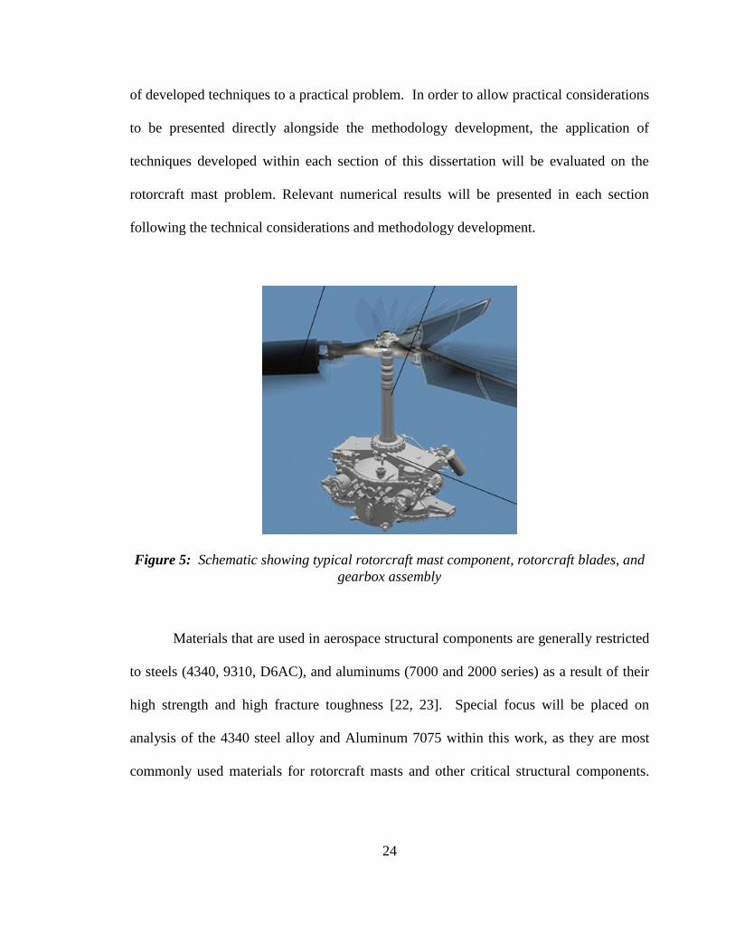
Figure 5: Schematic showing typical rotorcraft mast component, rotorcraft blades,
and gearbox assembly ............................................................................................... 24
Figure 6: Flow chart depicting dissertation outline and of methodology
development for stochastic fatigue crack growth evaluation .................................... 27
Figure 7: Fatigue crack growth rate threshold data for 4340 steel a.) raw data b.)
adjusted Ko data using Backlund equation [37] ...................................................... 34
Figure 8: Probability plot showing Adjusted Ko data to lognormal distribution
function ...................................................................................................................... 34
Figure 9: Histogram of Adjusted Ko data from experiment data and PDF of fitted
lognormal distribution function ................................................................................. 35
Figure 10: Adjusted Ko data from experiment data and CDF of fitted lognormal
distribution function .................................................................................................. 35
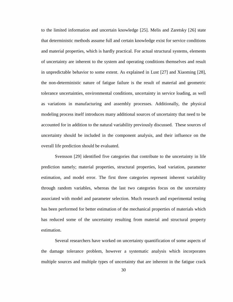
Figure 11: Typical S-N Curves for Steel and Aluminum materials .................................. 36
Figure 12: Fatigue Limit data for aluminum alloy 7075-T6 and fitted lognormal
distribution function .................................................................................................. 37
Figure 13: Stochastic fatigue crack growth curves using; a.) no correlation; b.) full
correlation; c.) partial correlation ............................................................................ 43
Figure 14: Probability plot showing Modified Paris parameter C data and
lognormal distribution function ................................................................................. 47
Figure 15: Histogram of Modified Paris parameter C calculated from experiment
data and PDF of fitted lognormal distribution function ........................................... 47

viii
Figure 16: Modified Paris parameter C calculated from experimental data and
CDF of fitted lognormal distribution function .......................................................... 48
Figure 17: Standard deviation of fatigue crack growth rate data .................................... 54
Figure 18: Ensemble of 5 stochastic fatigue crack growth curves generated using
partial correlation technique ..................................................................................... 55
Figure 19: (a.) Generated variable amplitude load history (b.) Graphical
representation of rainflow matrix showing cycle counts for discrete load levels
as calculated from (a) ................................................................................................ 60
Figure 20: Plot of histogram and fitted marginal PDF of load cycles from rainflow
matrix ......................................................................................................................... 61
Figure 21: Elements of the uncertainty quantification (UQ) procedure using
rainflow representation ............................................................................................. 62
Figure 22: Simple turning point load history .................................................................. 64
Figure 23: a.) Transition matrix b.) Transition probability matrix ................................. 65
Figure 24: Summary of typical results using proposed methodology ............................. 69
Figure 25: Monte Carlo simulation scheme for fatigue crack growth using proposed
methodology. ............................................................................................................. 69
Figure 26: Semi-Elliptical Crack showing crack length (2c) and depth (a)
definitions .................................................................................................................. 70
Figure 27: Plot of typical stress profile within rotorcraft mast component under
applied mixed mode loading ...................................................................................... 71
Figure 28: 10,000 calculated EIFS value and best fit lognormal distribution
function for Aluminum Alloy 7075-T6 ....................................................................... 73
Figure 29: Depiction of full model and sub model used in FEA for planar crack
analysis ...................................................................................................................... 75
Figure 30: Detailed view of finite element crack submodel volume a.) unmeshed
and b.) meshed configurations .................................................................................. 76
Figure 31: Schematic of GP training process using iterative greedy point algorithm .... 85
Figure 32: Relative order for cycles contained in 5x5 rainflow matrix ........................... 88
Figure 33: Original helicopter load spectrum.................................................................. 92
ix
Figure 34: Three reconstructed helicopter load spectra using the rainflow method ....... 92
Figure 35: Reconstructed helicopter load spectra using the Markov transition
method ....................................................................................................................... 93
Figure 36: Schematic of crack front showing Wheeler model parameters for plastic
zone based retardation correction ............................................................................ 96
Figure 37: Schematic showing sources of error during various stages of modeling
and simulation ......................................................................................................... 100
Figure 38: Histogram of Percent Errors found during full-model refinement
analysis with results compared to lognormal distribution ...................................... 106
Figure 39: Maximum GP model variance vs. # of Training points used ........................ 110
Figure 40: Plot showing simulated fatigue crack growth curves considering natural
variability, information uncertainty, and modeling error ....................................... 116
Figure 41: Plot showing mean and 90% confidence bounds on component life
prediction obtained using the a.) percentile b.) partial correlation crack
growth rate representations .................................................................................... 117
Figure 42: Typical fatigue crack profile showing crack growth due to fatigue
loading ..................................................................................................................... 118
Figure 43: a.) PDF and b.) CDF of Lognormal distribution function of number of
cycles to reach a critical crack size shown with simulation results ........................ 119
Figure 44: Schematic showing development of fracture surface for a.) in plane
crack opening subjected to mode I; b.) crack kinking under mode II; c.) crack
front twisting under mode III; d.) deflected crack for superimposed modes I, II,
and III ...................................................................................................................... 123
Figure 45: Forsyth's notation of fatigue crack growth evolution [143] ......................... 125
Figure 46: Typical stress intensity factor calculations along crack front obtained
using displacement correlation and M-integral methods. ....................................... 135
Figure 47: Work flow chart of FRANC3D/NG and finite element software for non-
planar fatigue crack modeling ................................................................................ 136
Figure 48: Non-planar crack growth analysis showing crack surface as well as
predicted and „best fit‟ crack extension locations ................................................... 138
Figure 49: Final crack configuration (surface profile) of initial horizontal surface
crack subjected to remote bending + torsion 2 block non-proportional loading.

x
The crack is seen to kink towards two primary kink angles, θ1 and θ2 depending
on applied loading ................................................................................................... 147
Figure 50: a.) submodel showing final kinked crack shape after non-planar crack
growth analysis; b.) submodel showing extraction of key flaw characteristics
for use in equivalent planar crack analysis ............................................................. 148
Figure 51: Isometric view of non-planar crack shape development showing initial
crack, kinked crack profile after 6 growth increments, and kinked crack profile
after 12 growth increments ...................................................................................... 154
Figure 52: a.) Plan and b.) Elevation view of non-planar crack shape development
showing initial crack, kinked crack profile after 6 growth increments, and
kinked crack profile after 12 growth increments (showing same crack profiles
as Figure 51) ........................................................................................................... 155
Figure 53: Simulated crack profiles using MTS (tensile only), MTS (tensile or
shear) and MSERR criteria for crack kink direction modeling a.) isometric
view; b.) plan view ................................................................................................... 158
Figure 54: SIF solution comparisons at different stages of crack propagation for
crack profiles obtained using different crack kink direction criteria.
Comparisons shown at a.) 0.1 b.) 0.5 and c.) 0.9 of normalized distance along
the crack front. ........................................................................................................ 159
Figure 55: Simulated crack profiles using MSS criteria for crack kink direction
modeling a.) plan view; b.) elevation view .............................................................. 161
Figure 56: a.) Full crack; b.) crack tip “A” surface profiles obtained from
numerical simulation showing crack shape development for 3 distinct load
sequences under 4 block variable amplitude loading conditions ............................ 163
Figure 57: a.) Full crack; b.) crack tip “A” surface profiles obtained from
numerical simulation showing crack shape development for 3 distinct load
histories with different loads and sequences under 4 block variable amplitude
loading conditions ................................................................................................... 165
Figure 58: Upper and lower bounds on crack front paths determined by performing
crack growth simulation under extreme load histories ........................................... 167
Figure 59: Comparison plots of stress intensity factor solutions found using non-
planar crack growth methodology and equivalent planar crack growth
methodology for CAL load case. Plots show SIFs along the crack front at a.)
0.1 normalized distance (near surface); b.) 0.5 normalized distance (depth); c.)
0.9 normalized distance (near surface) ................................................................... 170

xi
Figure 60: Comparison plots of stress intensity factor solutions found using non-
planar crack growth methodology and equivalent planar crack growth
methodology for 2 block VAL load case. Plots show SIFs along the crack front
at a.) 0.1 normalized distance (near surface); b.) 0.5 normalized distance
(depth); c.) 0.9 normalized distance (near surface) ................................................ 173
Figure 61: Comparison plots of stress intensity factor solutions found using non-
planar crack growth methodology and equivalent planar crack growth
methodology for 2 block VAL load case. Plots show SIFs along the crack front
at a.) 0.1 normalized distance (near surface); b.) 0.5 normalized distance
(depth); c.) 0.9 normalized distance (near surface) ................................................ 175

CHAPTER I
INTRODUCTION
1.1 Introduction
Mechanical components in engineering systems are often subjected to cyclic loads
leading to fatigue and progressive crack growth. It is essential to predict the performance
of such components to facilitate risk assessment and management, inspection and
maintenance scheduling, and operational decision-making. In 1978, the National Bureau
of Standards and Battelle Laboratories completed an exhaustive study that estimated the
total cost associated with material fracture and failure in the United States to be over $88
billion dollars per year (corresponding to almost 4% of the national GDP at the time) [1].
The study concluded that substantial material, transportation, and capital investment costs
could be saved if technology transfer, combined with research and development,
succeeded in reducing the factors of uncertainty related to structural reliability. Emphasis
on fracture mechanics, material properties, and improved inspection schedules/techniques
were identified as potential methods of improving structural reliability while reducing
material usage and replacement of critical components. Among the major industry sectors
where fatigue and fracture of structural components are of critical concern is that of the
aeronautical and aerospace industry.
Originally, the aeronautical community adopted the safe life design approach in
order to increase structural integrity throughout the design life of a component. Within
the safe life design method, components are assumed to be flaw free and are designed and

2
tested to withstand a pre-determined design life. The mean fatigue life of the structure is
estimated and then divided by a subjective safety factor in order to assure a safe operation
life of the component. Under this design philosophy, components are retired from service
following this safe life time period, regardless of their current condition. The
disadvantages of this approach are that components tend to be over-engineered, a large
percentage of components are retired long before their actual useful lives have been
reached, safety factors are not statistically evaluated, and the method does not account for
single “rogue” defects that could grow to a critical size during the design life. The
damage tolerance approach was later adopted in order to overcome some of these
limitations.
The U.S. Air Force became the first organization in the United States to formally
require damage tolerance design with the issuance of MIL-A-83444 Airplane Damage
Tolerance Requirements in 1974, which specifies that cracks shall be assumed to exist in
all primary aircraft structures [2]. Damage tolerance design is based on the assumption
that initial flaws (cracks, scratches, inclusions, etc) exist in any structure and such flaws
will propagate under repeated cyclic loading conditions which are substantially less than
the yield strength of the material, ultimately causing structural failure. Damage tolerance
concepts are based on fracture mechanics principles and have been pursued for fixed-
wing aircraft structures since mid 1970‟s [3]. This approach to structural analysis has
forced engineers to develop a more thorough understanding of relevant component
service loads and stress spectrums, material properties, and crack growth mechanisms.
Although significant work has been pursued for fixed wing aircraft over the past
few decades, relatively little work has been completed on its application to rotorcraft due

3
to complex component geometries, high cycle, low stress dynamic loading conditions,
and the necessity for accurate small crack, near threshold crack growth modeling.
Following a detailed assessment in 1999 by the Federal Aviation Administration (FAA)
and the Technical Oversight Group for Aging Aircraft (TOGAA) on the current
approaches to rotorcraft design for fatigue, the TOGAA recommended that a damage
tolerance philosophy should be used to supplement the existing safe-life methodology for
rotorcraft design and certification. In response to the assessment and recommendation,
the FAA initiated the process to revise FAR 29.571, Fatigue evaluation to include
damage tolerance requirements and developed a rotorcraft damage tolerance (RCDT)
R&D roadmap identifying multiple areas of research instrumental to development of
rotorcraft specific damage tolerance techniques and tools [4]. Much of the research
contained within this dissertation is motivated by the updated FAA RCDT initiative and
directly supports the critical research areas identified within the RCDT R&D roadmap
including, but not limited to, initial flaw state determination, fatigue crack growth
analysis, and risk assessment - probabilistic modeling.
The traditional damage tolerance (DT) approach to aircraft structures has assumed
a deterministic damage accumulation process where deterministic crack growth curves,
constant material properties, and specific initial flaw sizes are used. For DT-based design,
a safety factor is commonly used to ensure structural integrity. However, fatigue crack
growth is a stochastic process and there are different kinds of uncertainty – physical
variability, data uncertainty and modeling errors – that should be included within the
analysis to more accurately represent the fatigue life of the component. In order to
accurately assess the risk of failure of structural components, these sources of uncertainty

4
need to be identified and their statistical characteristics quantified. The probabilistic
method is more appropriate for damage tolerance analysis since it can properly account
for various uncertainties and assist the decision-making process with respect to design
and maintenance scheduling. Uncertainty appears at different stages of analysis and the
interaction between these sources of uncertainty cannot be modeled easily. Additionally,
the uncertainty quantification and propagation methodology must be developed to be
computationally efficient since the reliability assessment may require repeated evaluation
for accurate predictions.
The remaining sections within this chapter provide an overview of relevant topics
to fatigue crack growth analysis and will detail the research objectives and contributions
of this work. In order to provide a baseline level of understanding which is necessary for
later development and discussion, Section 1.2 reviews some of the major topics that are
relevant to crack growth analysis. Section 1.3 discusses some of limitations that exist in
the previous methodology and clearly states the main objectives of this research. A brief
summary of the major contributions contained in the subsequent chapters of this work
within the areas of uncertainty quantification and fatigue crack growth analysis is also
provided. Additionally, the demonstration problem to which the methods developed
within this work are applied is given within this section. The final section within this
chapter provides details on the overall organization of the subject material contained
within the remaining chapters of the dissertation.

5
1.2 Fatigue Crack Modeling Background
As mentioned previously, the damage tolerance approach can be utilized to ensure
that structural components have the capacity to withstand environmental loading even
under the presence of cracks or other defects. Inherent to this philosophy is the
underlying assumption that all structures have some initial flaws, which will propagate
under fatigue loading conditions. Linear elastic fracture mechanics (LEFM) based
methodologies have been used extensively to better characterize the fatigue crack growth
process in metals and are based on the application of classical linear elasticity to cracked
bodies. Linear elastic fracture mechanics theory is applicable for analysis of stable crack
growth resulting from repeated fluctuating loading conditions and can be used within the
damage tolerance approach to address structural integrity concerns by considering both
the damage propagation (growth) and the residual strength of the flawed component.
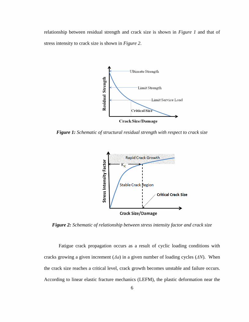
Residual strength is the amount of static strength of the structure available at any
time during a component‟s service life. The residual strength is expected to decrease
with increasing severity of damage. Plane strain fracture toughness is a material property
which describes the ability of a material containing a crack to resist fracture (rapid,
unstable crack growth), and is denoted by the parameter KIC. The structural safety of the
system of interest is maintained by ensuring that damage is never allowed to grow to a
sufficient size such that the stress intensity factor at the damage location exceeds KIC and
the residual strength of the system does not drop below the maximum in-service load
value. By enforcing these two conditions, it is possible to identify a critical crack size
over which the structural integrity of the system is insufficient. A schematic of the
6
relationship between residual strength and crack size is shown in Figure 1 and that of
stress intensity to crack size is shown in Figure 2.
Figure 1: Schematic of structural residual strength with respect to crack size
Figure 2: Schematic of relationship between stress intensity factor and crack size
Fatigue crack propagation occurs as a result of cyclic loading conditions with
cracks growing a given increment (Δa) in a given number of loading cycles (ΔN). When
the crack size reaches a critical level, crack growth becomes unstable and failure occurs.
According to linear elastic fracture mechanics (LEFM), the plastic deformation near the

7
crack tip is controlled by the stress intensity factor range (ΔK), and is applicable provided
the small scale yielding (SSY) condition is satisfied. The fatigue crack growth rate is
typically represented with the nonlinear functional relationship
,...,,,, aKKRKf
N
a
dN
dathIc
(1)
where da/dN is the crack growth rate per cycle, f is a non-negative function, ΔK is the
range of the stress intensity factor, R is the ratio between the minimum and maximum
applied loading, KIc is the plane strain fracture toughness, Kth is the threshold stress
intensity factor, and a is the crack length. KIc and Kth are both material properties and are
depicted within the schematic in Figure 3. The stress intensity factor (ΔK) is viewed as
the primary parameter, and is related to the applied loading, crack length, and geometry
of the component. Different empirical formulas have been proposed to represent some
portion(s) of the fatigue crack growth rate curve, with the Paris [5], Forman [6], and
Walker [7] laws given in Eqns. (2), (3), and (4) respectively.
m
KCdN
da (2)
KKR
KCf
dN
da
c
m
1 (3)
m
pR
KC
dN
da
1)1( (4)
The traditional fatigue crack growth rate curve is based on long crack behavior
and generally is sigmoidial in shape with three distinct regions; the near threshold, linear
8
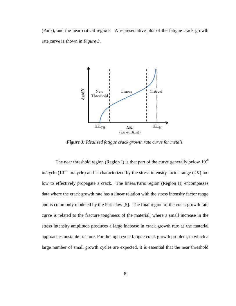
(Paris), and the near critical regions. A representative plot of the fatigue crack growth
rate curve is shown in Figure 3.
Figure 3: Idealized fatigue crack growth rate curve for metals.
The near threshold region (Region I) is that part of the curve generally below 10-8
in/cycle (10-10
m/cycle) and is characterized by the stress intensity factor range (ΔK) too
low to effectively propagate a crack. The linear/Paris region (Region II) encompasses
data where the crack growth rate has a linear relation with the stress intensity factor range
and is commonly modeled by the Paris law [5]. The final region of the crack growth rate
curve is related to the fracture toughness of the material, where a small increase in the
stress intensity amplitude produces a large increase in crack growth rate as the material
approaches unstable fracture. For the high cycle fatigue crack growth problem, in which a
large number of small growth cycles are expected, it is essential that the near threshold

9
region of the fatigue crack growth curve is accurately represented by the fatigue crack
growth model used in the analysis.
Table 1: Proposed fatigue crack growth models
Since the early 1960's when Paris [5] initially proposed the relationship between the
fatigue crack growth rate and the stress intensity factor range, many models have been
developed to represent the fatigue crack growth rate curve for various materials. Several
researchers have proposed different models of varying complexity including Forman [6],
Walker [7], Erdogan and Ratwani [8], among others. A more comprehensive, but far
from exhaustive, list of models is included in Table 1. As mentioned previously, for the
high cycle fatigue crack growth problem, in which a large number of small growth cycles

10
are expected, it is essential that the near threshold region of the fatigue crack growth
curve is accurately represented, and therefore future discussion will focus on those
models that meet this minimum requirement.
Under constant amplitude loading conditions, the fatigue life of the structure can
be found by simple integration of the fatigue crack growth rate model given in Eqn. (1).
However, most finite-life structures are subjected to random variable amplitude loading
while in service, which makes the fatigue life calculation significantly more difficult.
The most common method for dealing with crack growth propagation under variable
amplitude loading conditions is through the use of a cycle-by-cycle prediction method in
which the crack growth increment (da/dN) is evaluated for a given ΔK, and R
corresponding to each cycle within the variable amplitude history. However, relying on
a cycle-by-cycle calculation can become computationally expensive, particularly within a
probabilistic reliability analysis framework in which many life predictions must be
evaluated. This computational burden is again increased when a multiaxial variable
amplitude load is applied to a structure. Chapters 3 and 5 will further comment on the
challenges inherent to fatigue crack growth modeling under multi-axial variable
amplitude loading and will develop methods to address these issues for planar and non-
planar fatigue crack growth modeling within a probabilistic framework.
Since the damage tolerance methodology assumes an initial flaw/defect in the
material, and the key result of the analysis is focused on accurately predicting the number
of cycles for this initial crack to grow to a critical crack length. Key questions that need
to be addressed before crack analysis can be performed include:
1.) What initial crack shape should be used?

11
2.) What initial crack size should be used?
3.) How will crack propagation be modeled (single point, two-point, multiple
points along crack front)?
4.) What direction is the crack allowed to propagate (planar, non-planar)?
Although seemingly simple questions, clear answers are not always obvious and
can be problem dependent and subject to engineering judgment. Several different
approaches have been developed and reported within the literature to address each of
these issues, and the remaining portion of this section presents many of the methods that
have been used within previous research. However, most of these questions currently
remain open areas of research within the fatigue and fracture research community, where
improved methods and techniques are currently under investigation.
Most cracks and planar flaws can be classified within one of five general
categories: i.) surface-breaking flaws, ii.) through flaws, iii.) subsurface/embedded flaws,
iv.) corner flaws, and v.) edge flaws [9]. Although actual flaws contained within
structural components may have irregular shapes, these flaws are typically represented by
simpler, idealized shapes within crack growth studies. Two main factors are responsible
for the common practice of crack shape idealization; insufficient information of true
crack shapes within components and limited theoretical and modeling capabilities of
highly complex crack shapes. Most common nondestructive evaluation techniques are
incapable of characterizing detailed crack front profile, providing only limited crack
characterization information on crack size and location. Although advanced techniques
such as the scanning electron microscope (SEM) can be used to see microstructure level
defects, this technology is not widely available and can be expensive to operate.
12
Additionally, even if realistic crack front shapes were known, standard fracture
mechanics solutions as well as reliable crack front modeling capabilities are generally
only available for simple shapes. As a result, the shapes of surface, subsurface,
embedded, and corner flaws are typically represented as semi-elliptical, elliptical, and
quarter elliptical respectively, and through and edge cracks are generally assumed to have
a rectangular shape [9].
For any fatigue critical structural component, the smaller the initial crack size, the
higher the residual strength capacity, and the longer the overall fatigue life. Therefore, the
estimation of the initial flaw size is of critical importance. Several different methods are
available for determining initial crack sizes within as-manufactured components, and are
briefly discussed below.
If the size and shape of the true flaws can be identified using SEM or by some
other means, or if initial flaws are known to exist in the component (such as notches or
surface scratches), idealized crack sizes should be defined as the maximum extent of the
actual flaw [9]. That is to say, the idealized crack shape should fully inscribe the actual
shape, thus making the area of the idealized crack greater than that of the true crack
shape. In doing so, a larger crack size is assumed and a conservative fatigue life
prediction can be expected.
Another typical method for quantifying initial crack sizes within as-manufactured
material is by using nondestructive inspection techniques. Nondestructive inspection
(NDI) can be defined as the use of nonintrusive methods to ascertain the integrity of a
material or structure. Many different inspection methods have been developed to evaluate
the existence of flaws including liquid penetrant, magnetic particle, eddy current,

13
ultrasonic, and radiographic, among others [10]. NDI techniques are typically used on
fracture critical parts to detect flaws that are equal to or larger than a threshold crack
size. The threshold crack size is defined as the minimum crack size that can be
consistently detected using a given inspection method, and varies depending on the
inspection method used. Using information obtained from NDI techniques, engineers are
able to characterize initial flaw sizes based on the flaw sizes found within the inspected
components. Since NDI techniques are not capable of reliably detecting crack sizes less
than their threshold values, if no flaws are detected, engineers typically set the initial flaw
size as the minimum detectable flaw size for the specific NDI technique used. The U.S.
air force damage tolerant design handbook [11] reported ranges of approximate crack
lengths that are reliably detected using different NDI techniques, the results are
summarized in Table 2.
Table 2: Approximate limits of reliable crack size detectability limits
Solid Cylinder Hollow Cylinder
Specimen Type Straight Filleted Straight Filleted
Liquid Penetrant Lab 0.16 0.09 x 0.31
Production x x x x
Ultrasonic Lab 0.14 0.09 0.10 0.13
Production 0.14 0.07 x 0.13
Eddy Current Lab 0.20 0.23 x 0.14
Production 0.16 0.30 x x
Magnetic Particle Lab 0.12 0.07 0.10 0.13
Production 0.12 0.13 x x
* x represents cases where data was not reported
When no additional information is available for the characterization of initial flaw
sizes within a fatigue critical part, handbooks and standards can be used as references to

14
identify suitable values. Within the aerospace industry, the USAF damage tolerant
design handbook [11] specifies conservative initial flaw size assumptions for intact
structures. For edge cracks and corner cracks at holes the handbook suggests an initial
flaw size of 0.05 inches, whereas for through and surface cracks at locations other than
holes it suggests an initial half crack length (c) and depth of 0.125 inches (for surface
crack configurations in slow growth components). These values can be used for
subsequent fatigue life analyses.
The concept of equivalent initial flaw size (EIFS) has also been used for
determining the size distribution of initial cracks. The equivalent initial flaw size
approach has been used to derive initial flaw sizes from the distribution of fatigue cracks
occurring later in the service life of a component, typically using back extrapolation
techniques. Although mentioned here for completeness, the concept of EIFS will be
discussed in more detail within Section 3.2.
Several approaches, of various levels of sophistication, have been used within the
literature to extend the crack front of pre-existing flaws. Crack front extension at a single
point (surface), two points (along the semi-major and semi-minor axis locations
corresponding to surface and depth positions), or multiple points (all along the crack
front) have been used for 2D and/or 3D crack propagation. In selecting one of these
approaches for crack modeling, the engineer imposes one of three crack shape
development schemes, namely; circular, elliptical, or a general case.
For illustration, suppose an initial semi-circular surface crack is under
consideration. The usual method of dealing with propagating cracks is to assume that a
particular crack shape is maintained during the fatigue process. This is equivalent to a

15
single point extension modeling approach where the stress intensity factor is determined
at a single point (typically at the surface location where the highest stress intensity factor
is commonly found), and the entire crack front is extended by a single value [12
].
Implementing this approach will result in an initially circular crack remaining circular for
the entire duration of the crack modeling process. The next level of sophistication
considers crack growth at the semi-major and semi-minor axis locations [13] where the
stress intensity factors and crack growth are performed at the semi-major and semi-minor
axis locations only. Using this method an initial semi-circular crack may develop into an
elliptical surface crack if the crack growth rate at one location (surface or depth) is
calculated to be faster than the other point. In a general case, the crack front may be
divided into n points. For each point along the crack front, a stress intensity factor is
determined, crack growth rate is calculated and each point is extended accordingly [14].
This modeling approach allows an initially semi-circular crack to develop into a general
crack shape that may not necessarily be easily captured by a simple geometric shape (e.g.
semi-circular or semi-elliptical).
(a.) (b.)
Figure 4: Schematic of crack growth methods a.) semi-circular extension (constant along
crack front) b.) semi-elliptical extension (different crack extension at semi-major and
semi-minor locations)
16
Obviously, there exists a tradeoff between accurate/meaningful crack shape
evolution and crack modeling complexity. Although the multiple point advancement
scheme may provide the most flexibility in terms of crack shape development, it also
provides several additional modeling and computational complexities including multiple
stress intensity factors and crack extension computations, as well as complicated
remeshing requirements that simpler methods may avoid. It is mentioned here to make
the reader aware not only of the necessary considerations for accurate crack shape
representation, but also of the realistic computational limitations that exist for performing
fatigue crack growth propagation analysis within a probabilistic framework. These issues
will be discussed in later chapters as the crack modeling frameworks are developed for
both planar and non-planar analyses.
Fracture mechanics concepts provide the tools to enable fatigue life assessment of
structural components through crack growth analysis. In principle, the prediction of crack
growth using fracture mechanics requires the following steps:
(1) Identify the relevant crack growth properties (crack growth rate as a function
of the stress intensity factor, fatigue threshold, fracture toughness, etc) for the
material used in design
(2) Determine the initial flaw size, shape, and location
(3) Establish the cyclic stress time history
(4) Determine the stress intensity factor solution as a function of crack size,
shape, geometry, and loading
(5) Select a fatigue crack growth rate model and damage accumulation rule
17
(6) Propagate fatigue crack from initial flaw size to final (critical) flaw size
Each of these steps must be performed in order to obtain a prediction for the fatigue life
of a component, and several different methods and techniques which are available to
engineers, have been presented within this section. Inherent to each available method are
certain benefits, drawbacks, and limitations that must be considered when performing this
type of analysis. This research will focus on investigating various tools and techniques,
which are based on fundamental fracture mechanic principles, for fatigue crack growth
analysis under uncertainty.
The previous discussion within this section has focused on traditional,
deterministic fracture mechanics (DFM) principles and procedures. The DFM approach
assumes single, well defined, deterministic values for all model inputs. The result of the
deterministic approach is a single model prediction value. Traditional methods employing
deterministic approaches lack the ability to consider model predictions under uncertain
conditions and cannot answer “what-if” questions under operating or environmental
conditions which differ slightly from the values under which they were evaluated. In fact,
all the necessary inputs to a fracture mechanics analysis are rarely accurate to a high
degree of certainty, leaving the deterministic approach less than desirable [15]. To
overcome this limitation, engineers have used a worst-case scenario approach, in which
conservative values for all model inputs were assumed and used within a deterministic
analysis. If a system could perform safely under the worst-case conditions, then it also
would be functional under less severe load conditions. However, tradeoffs usually exist
between those factors that increase safety and those which increase performance or
economic considerations, and an optimal design for system safety under worst case

18
considerations may lead to an overdesigned structure with poor performance capabilities
(e.g. larger and thicker components have more strength, but result in increased vehicle
weight leading to decreased speed or maneuverability).
Probabilistic fracture mechanics (PFM) can be used to remove the unrealistic
conservatism that is inherent to the worst-case approach (i.e. simultaneous occurrence of
several improbable events), by combining known, assumed, or proposed statistical
variations of the controlling parameters within traditional engineering models [15].
Fracture mechanics and probability theory are implemented within the PFM framework
to account for both mechanistic and stochastic aspects of the fracture problem and PFM is
gaining popularity as a method for realistic evaluation of fracture response and reliability
of cracked structures [16]. PFM is based on the fundamental principles of deterministic
fracture mechanics but considers one or more of the input variables to be random rather
than having deterministic values. Therefore, rather than calculating a single fatigue life
prediction and using a safety factor based on engineering judgment, a range of fatigue life
predictions are calculated and appropriate values are selected to maintain a sufficiently
low, but cost effective, failure probability [17].
Early work using PFM in aircraft applications mainly focused on capturing the
inherent random nature in the applied loads or stresses in structural components. Much of
this work addressed crack initiation, rather than crack growth [18,19]. More recent work
has proposed additional methods in the area of PFM by treating various fracture
mechanics inputs as random variables (initial crack size, crack detection probability,
material properties, and service conditions [15]) with increased emphasis on crack
propagation methods. Examples of PFM analysis where certain input variables, such as
19
stresses, yield strength, and fracture strength, have been treated as random variables can
be seen in ref [15].
The failure probability at any given time may be determined by combining
conventional fracture mechanics calculations with an appropriate statistical approach.
Generally, the component failure is defined through some limit state function, g(…),
which defines the boundary between the region of safe operating conditions and that of
failure. Typically, the limit state function is expressed in terms of structural capacity and
structural demand. Failure is expected when the demand exceeds the capacity of the
system and is typically expressed as the limit state being < 0. The probability of failure is
the multiple integral of the joint probability density function in the region of failure (g(xi)
< 0) given by
n
D
nif dxdxxxfxgPP 11........0)( (5)
where D={(x1….xn): g(x1….xn) <0} is the region of failure, Pf is the probability of failure,
f(x1….xn) is the joint probability density function of the parameters x1….xn, and the
function g() is the limit state function defined above. The driving parameters, x1….xn, for
fatigue failure may be the component strength and the applied load, flaw size and critical
size, or stress intensity factor and fracture toughness [20]. Numerical based techniques
are then used to evaluate the failure probabilities of complex problems. Monte Carlo
simulation is broadly applicable to the generation of numerical results from PFM models
[21] and will be used within this work due to its scope, depth, and relative ease of
implementation for evaluating probabilistic component life predictions considering
multiple sources of uncertainty.

20
The probabilistic approach is capable of identifying the sources of variables
affecting the fatigue life and fatigue strength of the structure in terms of risk, while
eliminating the over-conservatism that maintains safety. It has been proven that the
probabilistic method can be extended to provide useful information to help managers in
making decisions regarding the operation and inspection time of the fleet in order to
maintain airworthiness [3]. The probabilistic method for damage tolerance analysis
presents the foundation on which this work is built and enables a systematic framework
for uncertainty quantification considering physical variability, data uncertainty, and
modeling uncertainty to be included within an overall component life prediction.
1.3 Problem Statement and Research Objectives
As the overall population of our aviation fleet (both fixed wing and rotary) ages
and existing aircraft are required to function long beyond their initial design life,
increasing emphasis has been placed on improving the understanding and modeling of the
fatigue crack growth problem. Amid ever shrinking budgets and resources, engineers are
tasked with the enormous responsibility of developing lower weight structures with
increased design lives, which still meet the high reliability requirements that have
become expected within the aviation industry. However, uncertainties exist at all levels of
the fatigue damage tolerance modeling process, resulting in unknown confidence bounds
on component life predictions made by engineers. In order to overcome this limitation, a
systematic framework for stochastic fatigue crack growth modeling must be developed
which accounts for uncertainty at all levels of the damage tolerance analysis. It is the goal

21
of this dissertation to provide a methodical and practical framework for quantifying
various sources of uncertainty and analyzing their effects on component reliability
predictions over time. The objectives of this dissertation are:
1.) Develop statistics based uncertainty quantification techniques for fatigue
crack model inputs and model parameters. Fatigue crack growth modeling
involves numerous input quantities such as initial flaw size, loading, and
material properties as well as various model parameters which should be
treated in a probabilistic manner. Each input may have a different form or use
within the fatigue modeling procedure and quantification must be performed
in such a way that additional new information can be easily incorporated into
the overall framework.
2.) Develop a methodology to perform fatigue crack growth analysis for
components subjected to multi-axial variable amplitude loading within a
probabilistic framework. The methodology must incorporate the random input
and parameter values which are quantified in the previous objective and
provide an accurate component reliability prediction over time. Uncertainty
quantification requires multiple analyses, therefore, the overall methodology
must also be computationally efficient to implement.
3.) Develop and implement necessary methods for quantification of error and
uncertainty in model predictions considering numerical solution error and
model form error. Each model within the crack growth process introduces
additional error, and this error must be accounted for and included within the
overall component reliability prediction.

22
4.) Implement methods developed in objectives 1, 2, and 3 for planar and non-
planar crack growth analysis. Three dimensional crack growth modeling
introduces additional uncertainties arising from model form (extension and
direction criteria) and numerical modeling approximations. These
uncertainties need to be evaluated from a statistical viewpoint and included
within the probabilistic fatigue life prediction.
Relatively little work has been completed on the application of the damage
tolerance method to rotorcraft structures due to their complex geometries, high frequency
dynamic loading, and mixed mode loading conditions. This research will help address
some of the limitations posed by the traditional damage tolerance modeling approach for
rotorcraft structures by further investigating the near threshold crack growth behavior and
material properties, overcoming small crack growth modeling restrictions, and
developing efficient computational methods which are suitable for mixed mode loading
conditions. These improvements to the current analysis methodology are developed to be
compatible with a probabilistic treatment of the fatigue crack growth process.
The overall goal of this research is to develop and implement an overarching
framework for fatigue crack growth under multi-axial, variable amplitude loading which
includes systematic uncertainty quantification at all levels of the fatigue crack growth
modeling process. Key contributions have been made to both planar and non-planar
crack growth analysis. A significant contribution contained within this work for planar
crack growth analysis is the development of a new framework for probabilistic fracture
mechanics which enables fatigue crack growth modeling under multi-axial, variable

23
amplitude loading conditions incorporating finite element analysis, surrogate modeling,
and cyclic crack growth modeling methods. Included in this area are novel approaches to
fatigue crack growth rate representation, surrogate model development, and model error
assessment. Contributions to the area of non-planar crack growth analysis include
uncertainty assessment in fatigue crack growth models resulting from the use of different
crack extension and direction criterion as well as an „equivalent planar‟ fatigue crack
growth modeling approach which reduces the computational expense of numerical
simulations while retaining valuable features of a full scale non-planar crack growth
analysis.
Demonstration Problem Description
The methods developed throughout this research will be applied to a
demonstration problem which is of general interest to the rotorcraft community. In
evaluating potential candidate problems several key characteristics were desired
including:
1. Metallic component
2. Principal structural element
3. Non-redundant part
4. Complex structural geometry
5. Subject to multiaxial, variable amplitude fatigue loading
6. Fatigue failure observed in the field
The rotorcraft mast structural component meets the above criteria and was identified as a
suitable demonstration problem that will be used throughout this research for application
24
of developed techniques to a practical problem. In order to allow practical considerations
to be presented directly alongside the methodology development, the application of
techniques developed within each section of this dissertation will be evaluated on the
rotorcraft mast problem. Relevant numerical results will be presented in each section
following the technical considerations and methodology development.
Figure 5: Schematic showing typical rotorcraft mast component, rotorcraft blades, and
gearbox assembly
Materials that are used in aerospace structural components are generally restricted
to steels (4340, 9310, D6AC), and aluminums (7000 and 2000 series) as a result of their
high strength and high fracture toughness [22, 23]. Special focus will be placed on
analysis of the 4340 steel alloy and Aluminum 7075 within this work, as they are most
commonly used materials for rotorcraft masts and other critical structural components.

25
Analysis results using data from other common aerospace grade materials will also be
shown on occasion.
Mixed mode loading conditions are known to exist within the mast structure.
Typically, tension, torsion, and bending forces are present during regular in-service
conditions. As the rotor system operates, upward thrust is generated by the blades and is
transferred to the rotorcraft body through the mast system. This causes tension loading to
exist within the mast system, and is the primary force that keeps the system air-born.
Torsion exists due to the twisting of the rotor system and the torque that is applied at the
top of the mast system from the rotating rotor blades. Finally, bending forces are
introduced as a result of the centrifugal force, resulting from the rotor system rotation,
which causes forces to act outward and perpendicular to the rotorcraft mast system.
Although all three loading conditions exist within the main rotor mast during in-service
conditions, tension typically only accounts for less than 5% of the overall applied loading
within the structure and can be deemed relatively insignificant for this problem. For this
reason, only bending and torsion are considered within this research, however, their
application does induce all three modes of loading (I, II, and III) within the cracked
structural component.
The rotorcraft mast component (and associated materials) will be referred to
throughout this work and will be used to demonstrate the applicability of methods for
probabilistic damage tolerance analysis presented in this research to a realistic structural
component.

26
1.4 Organization of the Dissertation
The content of this dissertation can be considered to address three major topics
with respect to the overall stochastic fatigue crack growth analysis process, namely;
quantification of the inherent uncertainty in model inputs, development of a flexible and
efficient fatigue crack growth propagation method, and quantification of the resulting
uncertainty in model outputs including modeling errors. A schematic showing the
various components of this work as related to the overall component fatigue life
prediction modeling approach is included in Figure 6.
The first topic is concerned with statistically quantifying model inputs and model
parameters. When individual variables are under consideration, statistical methods can
be used to fit probability density functions to experimental data sets. Chapter 2 addresses
uncertainty quantification techniques for parameters/processes that are common to both
the planar and non-planar crack growth methods. Additional sources of uncertainty that
are unique to the planar and non-planar crack growth analysis are addressed within
Chapter 3 and Chapter 5, respectively.
The second major topic covered within this dissertation focuses on developing a
framework to accurately model the fatigue crack growth process while including those
uncertainties which were previously identified and quantified. This task is addressed
within Chapter 3 for the planar fatigue crack growth modeling scenario and again in
Chapter 5 for non-planar crack growth analysis.
The last major topic analyzes the uncertainty of model outputs. Again, this topic
is addressed in two different chapters, corresponding to model output resulting from the
planar and non-planar fatigue crack modeling frameworks. Uncertainties in model

27
outputs are addressed in Chapter 4 and Chapter 6 for planar and non-planar crack growth,
respectively. Included in this topic is the quantification of modeling errors for each of the
models included in the overall crack modeling methodology. Discretization errors,
surrogate modeling errors, and various crack growth model form errors are identified and
statistically evaluated. Additionally, Chapter 6 analyzes the uncertainties in fatigue crack
shape and model prediction resulting from the use of different crack growth extension
and direction modeling criteria within the non-planar fatigue crack growth analysis
framework.
The final chapter summarizes the overall work contained within the dissertation
and provides recommendations for areas of future research.
Figure 6: Flow chart depicting dissertation outline and of methodology development for
stochastic fatigue crack growth evaluation

28
CHAPTER II
UNCERTAINTY QUANTIFICATION OF MODEL INPUTS AND PARAMETERS
2.1 Introduction
The reliability of an engineering system can be defined as the ability to fulfill its
design purpose for some time period [24]. For structural systems, reliability can be most
simply viewed as the capacity of the structure exceeding some demand. Typically
capacity is expressed in terms of structural strength, and demand is given by loads or
stress. Engineers are expected to design these systems so that the capacity of the structure
is maintained despite uncertainties in system performance over time (typically due to
degradation) and/or uncertain use and environmental conditions. Traditional engineering
approaches simplify the analysis by considering uncertain variables to be deterministic,
and then apply empirical safety factors on top of deterministic solutions. However,
empirical safety factors are typically based on past experience and/or engineering
judgment, and statistical justification for the choice of their values is not always
available. As a result, structural systems designed using empirical safety factors can be
either significantly overdesigned or operating at unacceptably low reliability levels.
The probabilistic approach to engineering design provides a method for
incorporating uncertainty within the structural analysis in a logical and meaningful way.
Uncertainty exists in the architecture, parameters, abstraction, and unknown aspects of an
engineering system. Additional uncertainty is introduced as a result of the predictive
models, simplifying assumptions, and analysis methods used [24]. Quantification of the

29
uncertainty inherent in each of these sources needs to be implemented within a structural
analysis to better understand the overall uncertainty within the analysis and how each
affects the overall variability in system performance.
Generally, uncertainties can be identified to be of two types; aleatory or
epistemic. Aleatory uncertainty can be defined as uncertainty arising from or associated
with the inherent, irreducible, natural randomness of a system or process. Additional
knowledge about this type of uncertainty is aimed not at reducing the uncertainty, but in
better quantifying the actual physical state of the system or process. Examples of
aleatory uncertainty are seen in material properties data and loading. Typically, a
probabilistic interpretation can be developed to capture this type of uncertainty assuming
enough statistically relevant data is available. Epistemic uncertainty is also known as
reducible uncertainty, or subjective uncertainty, and is associated with a general lack of
knowledge of the system or process under consideration. The epistemic uncertainty can,
in principle, be eliminated with sufficient study. However, for complex systems or
processes, this may not always be possible in practice. Typically, epistemic uncertainty
exists when there is non-existent, sparse, or incomplete experimental data, when multiple
plausible models are available or model approximations are made, when subjective expert
opinions/observations are used, and in any other cases where there exists a general lack
of information or knowledge about the behavior of the physical process or system.
Much of the traditional damage tolerance (DT) research has used deterministic
modeling approaches under well defined, simple loading conditions. Deterministic
fatigue failure analysis has been described as non-representative of the conditions during
flight, too conservative due to the application of generic safety factors, or inaccurate due
30
to the limited information and uncertain knowledge [25]. Melis and Zaretsky [26] state
that deterministic methods assume full and certain knowledge exist for service conditions
and material properties, which is hardly practical. For actual structural systems, elements
of uncertainty are inherent to the system and operating conditions themselves and result
in unpredictable behavior to some extent. As explained in Lust [27] and Xiaoming [28],
the non-deterministic nature of fatigue failure is the result of material and geometric
tolerance uncertainties, environmental conditions, uncertainty in service loading, as well
as variations in manufacturing and assembly processes. Additionally, the physical
modeling process itself introduces many additional sources of uncertainty that need to be
accounted for in addition to the natural variability previously discussed. These sources of
uncertainty should be included in the component analysis, and their influence on the
overall life prediction should be evaluated.
Svensson [29] identified five categories that contribute to the uncertainty in life
prediction namely; material properties, structural properties, load variation, parameter
estimation, and model error. The first three categories represent inherent variability
through random variables, whereas the last two categories focus on the uncertainty
associated with model and parameter selection. Much research and experimental testing
has been performed for better estimation of the mechanical properties of materials which
has reduced some of the uncertainty resulting from material and structural property
estimation.
Several researchers have worked on uncertainty quantification of some aspects of
the damage tolerance problem, however a systematic analysis which incorporates
multiple sources and multiple types of uncertainty that are inherent in the fatigue crack

31
growth modeling procedure has not been completed. In this chapter, focus will be placed
on statistically quantifying the model inputs and parameters that are particularly relevant
to the high cycle fatigue crack growth problem. Additionally, stochastic variable
amplitude loading conditions will be considered and addressed in an effort to more
realistically represent in-service loading conditions.
The remaining sections within this chapter focus on the uncertainty within model
inputs for fatigue crack growth analysis. Topics which are covered include uncertainty in
material properties, uncertainty in fatigue crack growth rate parameters, and uncertainty
in variable amplitude, multi-axial loading. Each source of uncertainty will be detailed
and suitable methods for quantification will be implemented and demonstrated for
rotorcraft damage tolerance analysis.
2.2 Uncertainty in Material Properties
Several researchers have attempted to address uncertainties in material properties
through statistical distribution functions. Among the material properties that have been
considered relevant to the fatigue damage tolerance analysis are the threshold stress
intensity factor, fracture toughness, ultimate tensile strength, and yield strength [30, 31,
32, 33, 34].
Threshold Stress Intensity Factor Range
Experimental data shows that the fatigue crack propagation rate tends to zero at
some critical value of the stress intensity factor, ΔK. The threshold exists because fatigue

32
crack growth rates of less than about one lattice spacing per cycle are not possible on
physical grounds [35]. The threshold stress intensity factor range, ΔKth, is the parameter
which defines separation between no crack growth and slow crack growth in the near
threshold region of the fatigue crack growth rate curve and is critical for accurately
assessing the fatigue lifetimes for components subjected to high cycle fatigue.
However, the threshold is not sharply defined [36], and has been shown to be
sensitive to loading factors, such as stress ratio, which is important when performing
analysis under variable amplitude loading conditions. The threshold stress intensity factor
tends to decrease with increasing R ratio and has been expressed by Backlund [37] to be
related to the stress ratio, R, and the threshold stress intensity factor at R=0, ΔKo, through
the relationship
o
d
oRth KRCK 1
(6)
where Co and d are fitting constants. For this relationship to be determined, it is essential
that the quantity ΔKo is available through experimental testing. Klesil and Lukas [38]
proposed a simpler version of Eqn. (6) by setting the constant Co=1. Barsom [39] further
simplified the expression by enforcing the fitting constant d to be set equal to 1. In cases
where the two fitting constants are not available, the value of Co = d = 1 will give
conservative results for the threshold stress intensity factor, ΔKth for R ≥ 0 [40], and will
result in the relationship:
oRth KRK 1 (7)
Under variable amplitude load conditions, it is necessary to properly account for
load ratio effects (min load/max load) that exist in experimental data prior to any

33
uncertainty quantification method. Rather than constructing distribution functions for
each of the threshold stress intensity factors obtained under different loading conditions,
it is preferable to first remove the underlying loading effects and quantify a baseline
material property that can be used for a variety of loading conditions. As a result, the
Backlund equation given in Eqn. (6) will be used within this work prior to distribution
fitting.
Fatigue crack growth rate data collected under different load ratios for Steel 4340,
representative of the material typically used in rotorcraft mast components, has been used
within this section for numerical investigation. A parametric study is first performed to
identify fitting parameter C and d for the Steel 4340 experimental data set with threshold
data collected at multiple R ratios. It was determined that C=0.4 and d=1 provided the
best results and effectively reduced data to single curve that could be used for baseline
analysis. Statistical distribution fitting techniques were performed to identify the most
appropriate distribution function for accurately representing the scatter found in the
threshold stress intensity factor experimental data.
The lognormal distribution was compared to the experimental data through the
chi-squared test, the Kolmogorov-Smirnov (K-S) statistical test at a 5% significance
level, as well as through traditional probability plot techniques as shown in Figure 8 [41].
The lognormal distribution function was found to accurately represent the data using all
three techniques. The histogram of the threshold stress intensity factor along with the
probability density function (PDF) of the fitted lognormal distribution are shown in
Figure 9, and the corresponding cumulative distribution function (CDF) is shown in
Figure 10. By quantifying the baseline condition without the effect of load ratio, the

34
fitted distribution function can be used, along with the Backlund equation (Eqn. (6)) to
sample statistical-based realizations of the baseline threshold stress intensity factor which
can be adjusted for particular load cases.
Figure 7: Fatigue crack growth rate threshold data for 4340 steel a.) raw data b.)
adjusted Ko data using Backlund equation [37]
3.6 3.8 4 4.2 4.4 4.6
0.0050.01
0.05
0.1
0.25
0.5
0.75
0.9
0.95
0.990.995
Data
Pro
babili
ty
Ko - Threshold data
Lognormal Distribution
Figure 8: Probability plot showing Adjusted Ko data to lognormal distribution function

35
3.6 3.8 4 4.2 4.4 4.60
0.2
0.4
0.6
0.8
1
1.2
1.4
1.6
1.8
Data
Density
Ko - Threshold data
Lognormal Distribution
Figure 9: Histogram of Adjusted Ko data from experiment data and PDF of fitted
lognormal distribution function
3.6 3.8 4 4.2 4.4 4.60
0.1
0.2
0.3
0.4
0.5
0.6
0.7
0.8
0.9
1
Data
Cum
ula
tive p
robabili
ty
Calculated Ko (Backlund: C=0.4)
Lognormal Distribution
confidence bounds (Lognormal Distribution)
Figure 10: Adjusted Ko data from experiment data and CDF of fitted lognormal
distribution function
Fatigue Limit
The fatigue limit has been traditionally used within the safe-life design
methodology as a means of matching the infinite fatigue life of specimen subjected to
36
low magnitude cyclic loading. The fatigue limit is the amplitude (or range) of cyclic
stress that can be applied to the material without causing fatigue failure [42]. The fatigue
limit has generally been determined through traditional S-N experiments, in which a
known stress is repeatedly applied to the specimen, and the number of cycles to failure is
recorded. Ferrous and titanium alloys tend to have a distinct fatigue limit, whereas other
materials, such as aluminum, tend to not have as well defined thresholds. Typically, for
these materials, the stress which corresponds to a value of 107 cycles is taken as a good
approximation for the fatigue limit of the material. The metallic materials properties
development and standardization (MMPDS) handbook [43] is recognized as a reliable
source of aircraft materials data from which accurate materials strength data and material
properties can be obtained.
Figure 11: Typical S-N Curves for Steel and Aluminum materials
However, performing material tests to define the fatigue limit of the material can
be time consuming and costly, because of the large number of cycles that must be applied

37
before structural failure is observed and the numerous test that are required to fully
capture the S-N curve. For this reason, sparse data may again exist for the statistical
quantification of the fatigue limit of the material of interest.
15 20 25 300
0.02
0.04
0.06
0.08
0.1
0.12
Fatigue Limit (Ksi)
Density
Data
Lognormal
Figure 12: Fatigue Limit data for aluminum alloy 7075-T6 and fitted lognormal
distribution function
When only sparse experimental data sets are available for distribution fitting
purposes, confidence in statistical quantities, such as mean and variance, may be
somewhat limited. That is to say, uncertainties may exist in the statistical fitting
parameters themselves. To overcome the limitations that sparse data pose to statistically
meaningful parameter estimation, resampling methods can be used. McDonald et al.[44]
proposed a method to account for data uncertainty, in which in the quantity of interest can
be represented using a probability distribution, whose parameters are in turn represented
by probability distributions. The accurate distribution representations of the fatigue limit
and the threshold stress intensity factor are important within this work as they are later
used for the numerical evaluation of the equivalent initial flaw size (EIFS) which
describes the statistical characteristics of the initial flaws sizes to be considered in the
material. Sparse experimental data is common for both of these material properties as a

38
result of the expensive and time consuming experimental tests which are necessary for
their determination. As a result, uncertainty may exist in the probability density
functions which are used to represent the statistical characteristics, which will directly
affect the statistical representation of other parameters which are derived from this
quantity, such as the equivalent initial flaw size (EIFS). The uncertainty resulting from
sparse data is addressed below and can easily be included within the overall uncertainty
quantification approach. Additional information on the specific EIFS formulation used
within this research is presented within Section 3.2.
A variety of resampling methods exist within the field of statistics, including both
bootstrapping and jackknifing. The bootstrap technique is a statistical method for
estimating the sampling distribution of an estimator by sampling with replacement from
the original sample set [45]. The jackknife technique is similar to bootstrapping, and can
be used to estimate the bias and standard error in a statistic, when a random sample of
observations is used to calculate it. The jackknife estimator technique systematically
recomputes the statistic estimate leaving out one observation at a time from the sample
set [46].
Consider a random variable X whose statistics are to be determined from
experimental data, given by x = {x1, x2 .. xn}. For the sake of illustration, suppose that the
random variable X follows a normal distribution, then the parameters (P) of this
distribution, i.e. mean and variance, of X can be estimated from the entire data set x.
However, due to sparseness of data, these estimates of mean and variance are not
accurate. Using resampling techniques such as bootstrapping method, jackknifing etc. the
probability distributions (fP(P)) of the parameters (P) can be calculated. Hence for each
39
instance of a set of parameters (P), X is defined by a particular normal distribution.
However, because the parameters (P) themselves are stochastic, X is defined by a family
of normal distributions. For a detailed implementation of this methodology, refer to
McDonald [44].
The current research uses similar resampling techniques to calculate the
distribution of the parameters (P), however does not define a family of distributions.
Instead, it recalculates the unconditional distribution of the random variable X [41]. The
probability density of X conditioned on the set of parameters (P) is denoted by fX|P(x).
The parameters are represented by the joint probability density fP(P). Hence, the
unconditional probability distribution of X (fX(x)) can be calculated as shown in Eqn.(8).
fxfxf PXX | P(P)dP (8)
The integral in Eqn. (8) can be evaluated through quadrature techniques or
advanced sampling methods such as Monte Carlo integration or Markov chain Monte
Carlo Integration. Hence, the unconditional distribution of X which accounts for
uncertainty in input data can be calculated. This method can be used to be able to better
characterize the distribution of threshold stress intensity factor (ΔKth) and fatigue limit
(Δσf) when only limited experimental data is available.
Yield Strength and Ultimate Tensile Strength
The probability distributions used to represent fracture toughness are also often
used to characterize the yield strength and ultimate tensile strength and include normal,
lognormal, and Weibull [47, 30]. In reality, these parameters may be variable and might

40
require probabilistic treatment. However, these properties are regularly monitored, have
tight manufacturing tolerances, and are easily tested by standard techniques. Therefore,
within this work it is assumed that these properties have limited uncertainties and will be
treated as deterministic values.
2.3 Uncertainty in Fatigue Crack Growth Rate Parameters
As mentioned previously, numerous crack growth rate empirical models have
been proposed within the literature. For the high cycle fatigue crack growth problem,
only those models which are capable of capturing the non-linear behavior within the
near-threshold region are relevant, since strictly linear models will drastically
overestimate crack growth rates within this region leading to unnecessarily short fatigue
life predictions. For the purpose of demonstration and general application of the methods
developed in the research, the modified Paris model [85] will be used as a result of the
multiple fitting parameters included in the model, the near threshold and linear region
modeling capabilities, and the familiarity of fatigue community with its functional form.
The modified Paris model is given by the relation:
p
thn
K
KKC
dN
da
1 (9)
By fitting crack growth rate models to available experimental data, it is observed
that natural scatter is seen in the data resulting in some fitting parameters remaining
relatively constant, while others tend to vary significantly. Stochastic parameters have
been introduced into various empirical crack growth models by Yang [48], Provan [49],

41
Moore [50], Cruse [51], and others to try to capture this phenomenon. By using
experimental data to fit model parameters to distribution functions, the uncertainties in
model parameters can be quantified. Various forms of probabilistic fatigue crack growth
models have been proposed, and can generally be divided into two distinct categories.
The first type of method accounts for the stochastic behavior in fatigue crack
growth data by treating the crack growth rates at specific stress intensity factors as
random variables that are completely uncorrelated to each other. This assumption is
equivalent to treating the crack growth process as a white noise process. This approach
will be referred to as the statistical FCG approach and results in the smallest statistical
variability (underestimates the variance) [52]. Yang‟s [48, 53] method using a hyperbolic
sine (SINH) fatigue crack growth model with an additional term representing a
homogeneous Gaussian random process fits into this category. By defining the
correlation function of the Gaussian random process equal to zero, the Gaussian term
represents a random white noise process. Although computationally feasible, this
approach artificially introduces randomness in the model prediction through a noise term,
and ignores the intuitive physical relationship that exists between stress intensity factor
and crack growth rate data. It has been inferred within the literature that the white noise
process is not valid for fatigue crack propagation, and therefore will not be included
within this research.
The second type of method treats coefficients of the deterministic crack growth
models as random variables. The statistics of the parameters are described using
common distribution functions, such as lognormal or Weibull distributions, and are
determined by fitting the model to available fatigue crack growth rate data. In numerous
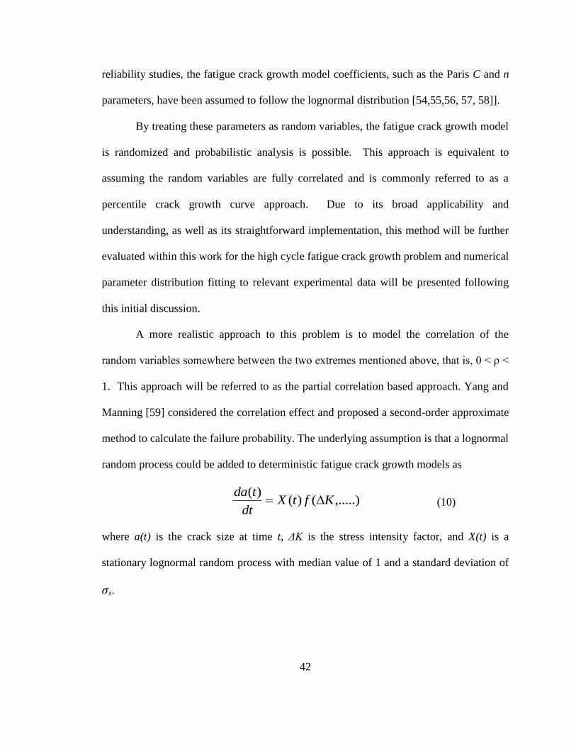
42
reliability studies, the fatigue crack growth model coefficients, such as the Paris C and n
parameters, have been assumed to follow the lognormal distribution [54,55,56, 57, 58]].
By treating these parameters as random variables, the fatigue crack growth model
is randomized and probabilistic analysis is possible. This approach is equivalent to
assuming the random variables are fully correlated and is commonly referred to as a
percentile crack growth curve approach. Due to its broad applicability and
understanding, as well as its straightforward implementation, this method will be further
evaluated within this work for the high cycle fatigue crack growth problem and numerical
parameter distribution fitting to relevant experimental data will be presented following
this initial discussion.
A more realistic approach to this problem is to model the correlation of the
random variables somewhere between the two extremes mentioned above, that is, 0 < ρ <
1. This approach will be referred to as the partial correlation based approach. Yang and
Manning [59] considered the correlation effect and proposed a second-order approximate
method to calculate the failure probability. The underlying assumption is that a lognormal
random process could be added to deterministic fatigue crack growth models as
,.....)()()(
KftXdt
tda (10)
where a(t) is the crack size at time t, ΔK is the stress intensity factor, and X(t) is a
stationary lognormal random process with median value of 1 and a standard deviation of
σx.

43
(a.)
(b.)
(c.)
Figure 13: Stochastic fatigue crack growth curves using; a.) no correlation; b.) full
correlation; c.) partial correlation

44
Liu and Mahadevan [52] have proposed a Karhunen-Loeve random process
expansion technique for stochastic SN analysis that accounts for realistic correlation
effects in fatigue damage accumulation simulation. The KL expansion technique is not
dependent on the Gaussian assumption and non-Gaussian methods for random field
representation are easily adopted. The KL expansion technique has been shown to agree
well with experimental data collected from various types of steel [52]. Some of the
benefits of approaching stochastic modeling by this approach are that the Gaussian
assumption is not necessary, the correlation is accurately represented to be 0 < ρ < 1, and
the variance is not restricted to a constant value.
Two distinct methods for probabilistic fatigue crack growth rate modeling are the
percentile and partial correlation based crack growth models. The percentile approach
offers a simple, straightforward method for representing the randomness seen in
experimental data, but may not realistically represent the correlation structure between
the stress intensity factor and the crack growth rate due to the method‟s implicit
assumption of a perfect correlation structure. The partial correlation based approach
overcomes this deficiency by providing the flexibility to represent any correlation value
between 0 and 1, however, in doing so, adds model complexity in the form of
representation and implementation. Each of the methods provides a benefit to the analyst,
and, therefore, both are implemented within this work and are presented below. First,
the percentile crack growth method is detailed and statistical distributions are fit to
common fatigue crack growth model parameters using experimental data. Following the
discussion of the percentile based approach, a partial correlation based method is
presented and implemented for the same experimental data set. The methodology
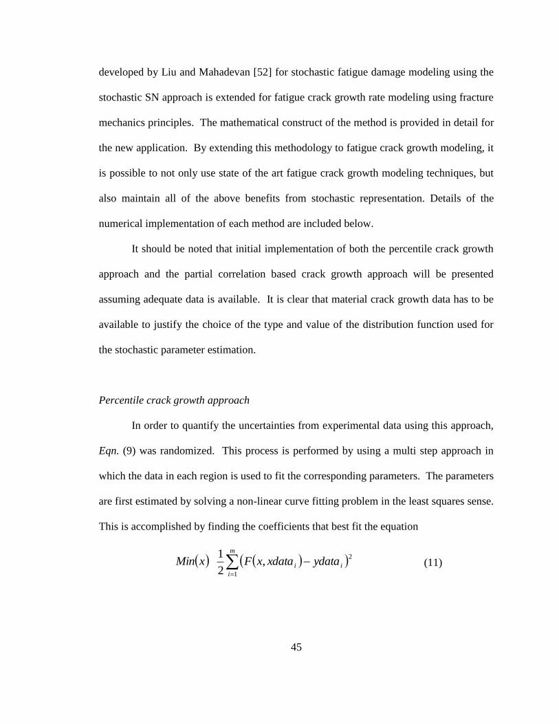
45
developed by Liu and Mahadevan [52] for stochastic fatigue damage modeling using the
stochastic SN approach is extended for fatigue crack growth rate modeling using fracture
mechanics principles. The mathematical construct of the method is provided in detail for
the new application. By extending this methodology to fatigue crack growth modeling, it
is possible to not only use state of the art fatigue crack growth modeling techniques, but
also maintain all of the above benefits from stochastic representation. Details of the
numerical implementation of each method are included below.
It should be noted that initial implementation of both the percentile crack growth
approach and the partial correlation based crack growth approach will be presented
assuming adequate data is available. It is clear that material crack growth data has to be
available to justify the choice of the type and value of the distribution function used for
the stochastic parameter estimation.
Percentile crack growth approach
In order to quantify the uncertainties from experimental data using this approach,
Eqn. (9) was randomized. This process is performed by using a multi step approach in
which the data in each region is used to fit the corresponding parameters. The parameters
are first estimated by solving a non-linear curve fitting problem in the least squares sense.
This is accomplished by finding the coefficients that best fit the equation
m
i
ii ydataxdataxFxMin1
2,
2
1 (11)

46
given input data xdata, and the observed output ydata, where xdata and ydata are vectors
of length m, and F(x,data) is a vector-valued function. After the parameters have been
estimated, some are held as constants while others are assumed to be random variables.
For each data point within a given data set, a realization of the random variable is
obtained, and, after all the realizations are collected, the parameter can be fitted to a
probability distribution. In order to choose the best fit for a given distribution, the
Anderson-Darling (A-D) statistic is used. The main fitting parameters corresponding to
the linear region of the Modified Paris fatigue crack growth model are C and n shown in
Eqn. (9). Using the non-linear curve fitting procedure outlined above, data within the
linear region could be used to evaluate Eqn. (11) to determine the best values for the
parameters C and n. After estimates for both parameters where obtained, n was held at its
mean value, and realizations of C were obtained for each data point within the data set.
The experimental data fitting results could then be fit to a well defined distribution
function.
Experimental fatigue crack growth rate data collected for Steel 4340 is included
for demonstration purposes. The analysis is limited to only the fatigue crack growth rate
data that corresponds to the linear region of the crack growth rate curve (see Figure 3).
The experimental data is analyzed to determine the statistical distributions of fatigue
crack growth rate model parameters corresponding to the linear region of the curve. The
results from this numerical study are presented here to demonstrate uncertainty
quantification of fatigue crack growth model parameters, and the uncertainty
quantification results obtained here are applied to the overall probabilistic fatigue crack
growth modeling analysis presented in Chapter 3.
47
1 1.5 2 2.5 3 3.5 4 4.5 5 5.5 6
x 10-9
0.00050.001
0.0050.01
0.05
0.1
0.25
0.5
0.75
0.9
0.95
0.990.995
0.9990.9995
Data
Pro
babili
ty
Modified Paris "C" data
Lognormal Distribution
Figure 14: Probability plot showing Modified Paris parameter C data and lognormal
distribution function
1 1.5 2 2.5 3 3.5 4 4.5 5 5.5 6
x 10-9
0
1
2
3
4
5
6
x 108
Data
Density
Modifed Paris "C" data
Lognormal Distribution Fit
Figure 15: Histogram of Modified Paris parameter C calculated from experiment data
and PDF of fitted lognormal distribution function

48
1 1.5 2 2.5 3 3.5 4 4.5 5 5.5 6
x 10-9
0
0.1
0.2
0.3
0.4
0.5
0.6
0.7
0.8
0.9
1
Data
Cum
ula
tive p
robabili
ty
Modified Paris "C" data
Lognormal Distribution
confidence bounds (Lognormal Distribution)
Figure 16: Modified Paris parameter C calculated from experimental data and CDF of
fitted lognormal distribution function
Statistical goodness of fit tests are used to analyze the experimental results with
theoretical distribution functions. Several common distribution functions were compared
to the experimental data set and it was determined that the lognormal distribution well
characterized the data. The lognormal distribution was compared to the experimental data
through the chi-squared test, the Kolmogorov-Smirnov (K-S) statistical test at a 5%
significance level, as well as through traditional probability plot techniques, and was
found to pass all of the statistical tests considered. The numerical analysis revealed that
the fatigue crack growth parameter C could be well characterized by the lognormal
distribution function with a mean value of 2.4378*10-9
and a standard deviation of
8.074*10-10
, corresponding to a coefficient of variation (COV) of approximately 0.33.
For the high cycle fatigue crack problem, it is not only necessary to capture the
uncertainty in the linear region of the fatigue crack growth rate curve, but also critical to
incorporate the uncertainty in the near threshold region. Similar to the statistical method

49
outlined above for the linear region parameters C and n, so too can the statistics of the
model parameters in the near threshold region be treated as random variables. The main
parameters corresponding to the near threshold region of the Modified Paris fatigue crack
growth model are ΔKth and p shown in Eqn. (9).
The parameter p in Eqn. (9) is used to help capture the transition from the near
threshold to the linear region of the fatigue crack growth rate curve. The transition from
the near vertical threshold region to the sloped linear region appears smoother and more
gradual when p increases, and becomes increasingly sharp as p decreases. Values of p
found for aerospace grade aluminum and steel materials are generally ≤ 1. When
compared to experimental data, it is seen that the gradient of the fatigue crack growth rate
in the transition zone from the near threshold to linear region appears consistent,
indicating that p can be treated as a deterministic value. As a result, p is treated as an
empirically fitted deterministic constant within this dissertation and can be best fit using
the least squares method outlined above.
The other primary parameter within the near threshold region is the threshold
stress intensity factor, ΔKth. The threshold stress intensity factor range, ΔKth, is the
parameter which defines separation between no crack growth and slow crack growth in
the near threshold region of the fatigue crack growth rate curve. ΔKth should be treated as
a random variable and a detailed discussion of its significance as related to the high cycle
fatigue problem as well as appropriate techniques for statistical characterization has been
previously included in Section 2.2. It was found that the baseline near-threshold stress
intensity factor (lacking load ratio effects) for steel 4340 could be well represented by the
lognormal distribution function as shown in Figure 8, Figure 9, and Figure 10 in Section

50
2.2. The reader is encouraged to refer to the previous section for additional details and
discussion on this topic.
Methods to fit model parameters from fatigue crack growth rate models to
statistical distribution functions using experimental data sets has been presented. Crack
growth rate models within the near-threshold and linear regions should be analyzed
separately using only experimental data contained in the region which is relevant to the
model parameters. It was found that for the 4340 steel data set which was considered, the
lognormal distribution function provided the best fit for both the C and Kth parameters
contained in Eqn. (9). However, it should be noted that different distribution functions
such as Normal, or Weibull distributions may provide a better fit when considering
different datasets or different materials, and the most accurate distribution function
should be used within subsequent analysis. The framework proposed within the following
chapter is flexible and allows for the use of any distribution function for the
representation of fatigue crack growth rate model parameters.
Once the crack growth rate parameters are fit to distribution functions, the
percentile approach offers a simple, straightforward method for representing the
randomness seen in experimental data by treating the stress intensity factor and fatigue
crack growth rate as perfectly correlated random variables. The result of this assumption
is shown schematically in Figure 13 b. Uncertainty in fatigue crack growth rate data can
be captured using this technique by randomly sampling the statistical distributions of
each random parameter for each fatigue crack growth analysis performed.

51
Partial Correlation based crack growth approach
The partial correlation based crack growth approach treats the crack growth rate at
any specific stress intensity factor as a random variable and a stochastic process modeling
method is used to avoid the assumption that crack growth rates at different stress intensity
factors are either completely correlated or completely uncorrelated as previously
developed methods assume [52]. The method detailed below is an extension of a stress
life (SN) based approach developed by Liu and Mahadevan [52] and details of the
methodology as they relate to crack growth modeling using fracture mechanics principles
is included below.
Within this section, for the sake of illustration, the fatigue crack growth rates at
given stress intensity factors are assumed to follow the lognormal distribution. The
lognormal assumption makes log(da/dN(ΔK) a Gaussian process with a mean value
process of E[log(da/dN(ΔK)] and a standard deviation of σlog(da/dN(ΔK). It should be noted
that non-Gaussian methods for random field representation are available, and that the
Gaussian assumption is not a requirement, but has been made to simplify the discussion
[52]. The mean value, E[log(da/dN(ΔK)], is representative of the mean da/dN vs. ΔK
curve found through deterministic analysis. The mean curve can be found using any
available general crack growth model.
It can be seen within experimental data that the variance of da/dN is not constant,
but rather is a function of stress intensity factor range, ΔK. Significant scatter may exist in
both the near threshold and linear crack growth regions. If σlog(da/dN(ΔK) represents the

52
scatter in the data, then the process given by Eqn. (12) is a normal Gaussian process with
zero mean and unit variance.
))(/log(
))])(/[log())(/(log()(
KdNda
KdNdaEKdNdaKZ
(12)
The random process, Z(ΔK), can be expressed using the Karhuenen-Loeve
expansion technique [60, 61] as a sequence of statistically independent random variables.
Generally, the expansion is expressed as
)()()(1
KfKZ ii
i
i
(13)
where )( i is a set of independent random variables, and i and )( Kfi are the ith
eigenvalues and eigenfunctions of the covariance function C(ΔK1,ΔK2), evaluated by
solving the homogenous Fredholm integral equation analytically or numerically. The
homogenous Fredholm integral equation is given by
)()(),( 1221 KfKfKKC iii
D
(14)
The autocovariance function, C(ΔK1,ΔK2), can be expressed through the
exponential decay function of Z(s) as:
||
2121),(
KKeKKC
(15)
where μ is a measure of the correlation distance of Z(ΔK) and depends on the material.
Through the control of the parameter μ, the exponential decay function can model
covariance structures ranging from fully correlated (μ 0) to fully uncorrelated (μ
+∞). These two extreme cases correspond to the percentile and statistical stochastic
models respectively.

53
Based on Eqns. (13) through (15), the fatigue crack growth rate can be modeled
as:
))])(/[log(*)()())(/(log( ))(/log(
1
KdNdaEKfKdNda KdNdaii
i
i
(16)
This equation not only expresses the fatigue crack growth rate as a function of ΔK
through the deterministic mean term, but also includes terms from the KL expansion
which introduces stochastic behavior in the crack growth prediction and captures the
correlation structure. A typical fatigue crack growth curve representation which is
obtained after applying this method can be seen in Figure 13 (c). Only a finite number of
terms within the KL expansion are necessary to effectively model the stochastic behavior
seen in most practical applications. Usually, 10-20 terms suffice for providing
sufficiently precise results under the standard Gaussian assumption [52].
Since da/dN increases with increasing stress intensity factor range, ΔK, it is a non-
stationary random process. In order to accurately model the variance of da/dN over the
entire range of ΔK values, the crack growth rate curve can be subdivided into n sections
(or regions), with the variance determined within each section from experimental data.
As the number of sections, n, increases, the general trend of variance of da/dN over the
range of ΔK values can be determined and can be closely approximated by a common
functional form (linear, power, etc). Once the variance is determined, the standard
deviation (σ) can easily be found and used within Eqn. (16). Figure 17 shows the
standard deviation determined over the each interval of da/dN (standard deviation
evaluated from data within each order of magnitude) for data collected under several

54
different R-ratios for 2024-T3 Aluminum alloy. As can be seen in the figure, the
standard deviation appears to be independent of R ratio, thus allowing it to be modeled by
a single function for all R ratios.
10-9
10-8
10-7
10-6
10-5
10-4
10-3
10-10
10-9
10-8
10-7
10-6
10-5
10-4
10-3
Standard Deviation vs. da/dN
da/dN (inches/cycle)
Sta
nd
ard
De
via
tio
n
Linear Fit
R=0
R=0.5
R=0.7
Figure 17: Standard deviation of fatigue crack growth rate data
Figure 18 shows 5 realizations of the fatigue crack growth rate curve obtained by using
the partial correlation method along with experimental crack growth rate data. A random
realization of the fatigue crack growth curve can be generated for each simulation within
the overall stochastic fatigue crack growth modeling framework.

55
101
10-8
10-7
10-6
Delta K (ksi-sqrt(in))
da/d
N (
in/c
ycle
)
Stochastic Realization 1
Stochastic Realization 2
Stochastic Realization 3
Stochastic Realization 4
Stochastic Realization 6
Experimental FCGR data
Figure 18: Ensemble of 5 stochastic fatigue crack growth curves generated using partial
correlation technique
Either the partial correlation method or the percentile fatigue crack growth rate
modeling approach can be used to represent the variability that exists in experimental
fatigue crack growth rate data. Additionally, each can be easily incorporated within an
overall crack growth probabilistic analysis. However, the partial correlation based fatigue
crack growth rate modeling approach using a K-L expansion technique offers several
advantages over previous methods, including:
1.) More realistic correlation structure representation of the crack growth rate at
different stress intensity factor ranges
2.) Can be used to exactly model statistical and percentile crack growth
representations
3.) Capability of modeling Gaussian and non Gaussian stochastic behavior
56
4.) Flexibility to include changes in variance within specific regions of the crack
growth rate curve as dictated by the data set under consideration
The partial correlation method for representation of fatigue crack growth rate data can be
used within a Monte Carlo simulation method for stochastic fatigue crack growth
prediction in order to account for the natural scatter observed in experimental fatigue
crack growth rate data.
2.4 Uncertainty in Variable Amplitude, Multi-axial Loading
As part of the certification process for rotorcraft and fixed wing aircraft, assumed
design load spectra must be verified on the basis of actual flight load measurement. These
lengthy, irregular time histories contain the fatigue relevant load information that is
necessary for life prediction. Measured time histories contain all of the information about
the loading history including all phasing, frequency, sequence, magnitude, and mean
effects [62], however they contain so much data that they are difficult to decipher and
compare. In order to accurately characterize load histories in a meaningful way, the
content of a measured signal must be able to be summarized and quantified in an efficient
and concise way [63]. Various methods exist to quantitatively assess recorded time
histories, and are generally grouped into two distinct categories; frequency domain
methods and time domain methods [35].
Different harmonic analysis methods can be used to determine the “frequency
content” of the signal by characterizing the frequencies or wavelengths of the built up

57
signal. Although some research has been published that uses traditional frequency
domain based methods for fatigue evaluation [64,65], such analysis is generally relevant
only to determine the vibration characteristics of the structure, and is not very descriptive
of the fatigue damage of the loading [63].
It is generally agreed that the structural load variations used in metal fatigue
analysis should be characterized in the time domain since it is the maxima and minima,
and the number of cycles (rather than time) which are the main controlling parameters
[35, 66], and the shape of the intervening curve between a maximum and a minimum is
of little importance [67]. Time domain methods typically work by identifying
occurrences of specific “events” in a load-time sequence. Typical events of interest
include the occurrence of load peaks/maximums at specific levels, the exceedance or
crossings of specific levels, and the occurrence of load changes or ranges of a specific
size [63]. Methods which help identify fatigue relevant “events” within a complex load
history are generally referred to as simply counting methods. Many counting techniques
are available including: level crossing, peak count, mean crossing peak count, range
count, and range-pair counting techniques [68,69], however, the rain-flow counting
method (range pair-range) is widely recognized as the most accurate and meaningful way
of representing variable amplitude loading [66].
It is obvious that in-service operational loading on many structures is a stochastic
process and typically cannot be adequately characterized by a single constant or variable
amplitude load history. Statistical investigation of the variable amplitude load cycle
distribution is often a critical task, as the structural reliability under service loading has
strong dependence on the accurate quantification and representation of such loads. The

58
majority of research has been performed under constant amplitude conditions, and only
limited effort has been put into developing statistical tools for fatigue load
characterization when the loads are both variable amplitude and stochastic [70]. An
efficient and accurate method is needed for quantification and characterization of the
fatigue content (load reversals) contained within a variable amplitude load spectrum.
Additionally, methods are needed to capture and represent the inherent uncertainty that
exists within the environmental loading condition.
Several counting techniques are discussed in detail below and implemented in this
research for initial load quantification purposes. Load characterization using the rainflow
counting method is presented first, followed by methods using the Markov method. The
results obtained from each of these methods are later used within Chapter 4 to generate
stochastic load simulations with similar loading characteristics as the original measured
history within a probabilistic crack growth framework.
Load Quantification using Rainflow Counting Method
The majority of the previous research that includes rainflow counting methods has
been used in combination with the stress-life (S-N) or strain-life (ε-N) methods [69] in
which the damage in each cycle is computed based on data gathered from constant
amplitude tests using a damage accumulation rule such as Miner‟s Rule. This research
uses the rainflow counting method as an initial fatigue loading quantification method and
then implements a stochastic regeneration technique for variable amplitude load spectrum
simulation which can be used within a fracture mechanics based crack growth analysis
procedure. The load quantification method using the rainflow cycle counting procedure

59
will be presented within this section, whereas the stochastic generation of additional load
histories will be presented later in Chapter 3.
The rainflow method was originally proposed by Matsuiski and Endo [71], and is
viewed by many to be the most popular and best method of cycle counting. The method
separates high and low amplitude load cycles and records them in a physically
meaningful way. To briefly summarize the method, for each local peak (smax) within the
time history, the rainflow algorithm finds the corresponding local trough (smin) to form a
hysteresis loop. The stress range as well as the mean stress for each cycle is determined,
and the results are stored in matrix form. In this way, the complex load history is reduced
to a simple rainflow matrix which contains information about the stress amplitudes, mean
values, and number of occurrences of each loading cycle. Additional details of the
rainflow counting method are available in various literature sources [68, 69].
The objective of the rain-flow method or the range pair-range method is to
extract and count cycles of various sizes. These load cycles are considered to be the basic
elements of a load sequence. The final counting result is contained in a matrix A of size
(k+1) x (k+1), in which the element aij gives the number of counted cycles from load
level i to load level j, and k is a user defined number of discretization levels, usually set
to 32, 64, or 128 depending on accuracy and computational efficiency desired [72,73].
Plots of a generated load history signal and its corresponding rainflow matrix are shown
within Figure 19.

60
0 5000 10000 150000
5
10
15
20
25
30Variable Amplitude Load History
Load (
Ksi)
(a.) (b.)
Figure 19: (a.) Generated variable amplitude load history (b.) Graphical representation
of rainflow matrix showing cycle counts for discrete load levels as calculated from (a)
Although cycle counting methods have typically been viewed as deterministic
methods for characterizing load histories, the obtained results from such methods can be
easily transformed for use within a statistical framework in one of two ways. The first
method simply uses the counted load cycles within the rainflow matrix within a
stochastic regeneration technique to produce random fatigue load history simulations.
The second method fits the elements in the rainflow matrix to a joint distribution, for full
statistical representation of the loading characteristics. In order to accomplish this, both
the "from" load level and "to" load level within the rainflow matrix are considered as
random variables, say x and y, respectively. Assuming that the rainflow counting results
are discrete values, the joint probability mass function (PMF) of x and y is denoted as
),(, yxp YX and the joint cumulative distribution function (CDF) given by [74]:
xx yy
jiYXYX
i j
yxpyxF ),(),( ,, (17)

61
The variables x and y can also be approximated as continuous variables with their joint
PDF denoted by ),(, yxf YX and the joint CDF given by:
dvduvufyYxXPyxF
x y
YXYX
),(),(),( ,, (18)
The histogram of extracted values as well as the marginal PDF (obtained from the
rainflow matrix shown in Figure 19 is shown in Figure 20.
Figure 20: Plot of histogram and fitted marginal PDF of load cycles from rainflow
matrix
A schematic of the procedure for the uncertainty quantification of the variable
amplitude load spectrum is shown in Figure 21. By using the rainflow counting
procedure in combination with statistical distribution fitting techniques, a complex load
history can be easily broken down into its elementary cycles and efficiently represented
by a joint probability density function.

62
Figure 21: Elements of the uncertainty quantification (UQ) procedure using rainflow
representation
Load Quantification using Markov Chain Method
The Markov method uses the loading information contained within a
representative fatigue cycle history to construct a probability based transition matrix.
The transition matrix contains discretized load levels with the "from" load level and "to"
load level composing the axes, and is populated by placing all level transitions contained
within the stress history in the discrete (i,j) position according to the nominal stress
values (σi, σj) that they represent.
For a realistic loading history, not only the load amplitude at a certain time
instance is random, but also the load amplitudes at adjacent time instances may be
correlated, i.e., the amplitude at time instance Tk can affect the amplitude at time instance
Tk+1. Given this assumption, the fatigue loading history with m discrete load levels are
Rain-flow counting
Distribution Fitting of Rainflow Matrix
UQ using Rainflow Counting
Representative VAL History
Marginals & Joint Distribution
Stochastic Reconstruction

63
modeled as a discrete time Markov chain {Xn}, which is a Markov stochastic process
whose state space (the set of discretized load levels) is a finite set, and for which n is a
discrete time instance ( n = T0, T1, T2, …, ) [75]. Let event Ek,i denote that the loading
amplitude at time instance Tk equals to load level i, and let event Ek+1,j denotes that the
loading amplitude at Tk+1 equals load level j. With a further assumption that the one-step
transition is independent of time instances, i.e., the transition between Ek,i and Ek+1,i
depends on i and j only, and not on previous values, a stationary Markov chain transition
matrix is constructed as:
0
0
0
0
1,1,
,1
1,2
,12,1
nnn
nn
n
II
I
I
II
I
(19)
where Ii,j is the one-step stationary transition count between Ek,i and Ek+1,i, which can be
obtained directly from the original load spectrum. The elements above the main diagonal
in I represent the transitions from minima to maxima, whereas the elements below the
main diagonal represent the transition from maxima to minima.
Given a load spectrum with discrete load levels from time T0 to Te, the element of
the stationary Markov chain transition probability matrix Pi,j can be estimated using the
number of occurrences of that the event Ek,i is followed by the event Ek+1,i, i.e.,
1
0
,, )(e
k
jiji kIC (20)
jiCC
jiCC
Pi
j
jiji
m
ij
jiji
ji 1
1
,,
1
,,
,
/
/
(21)
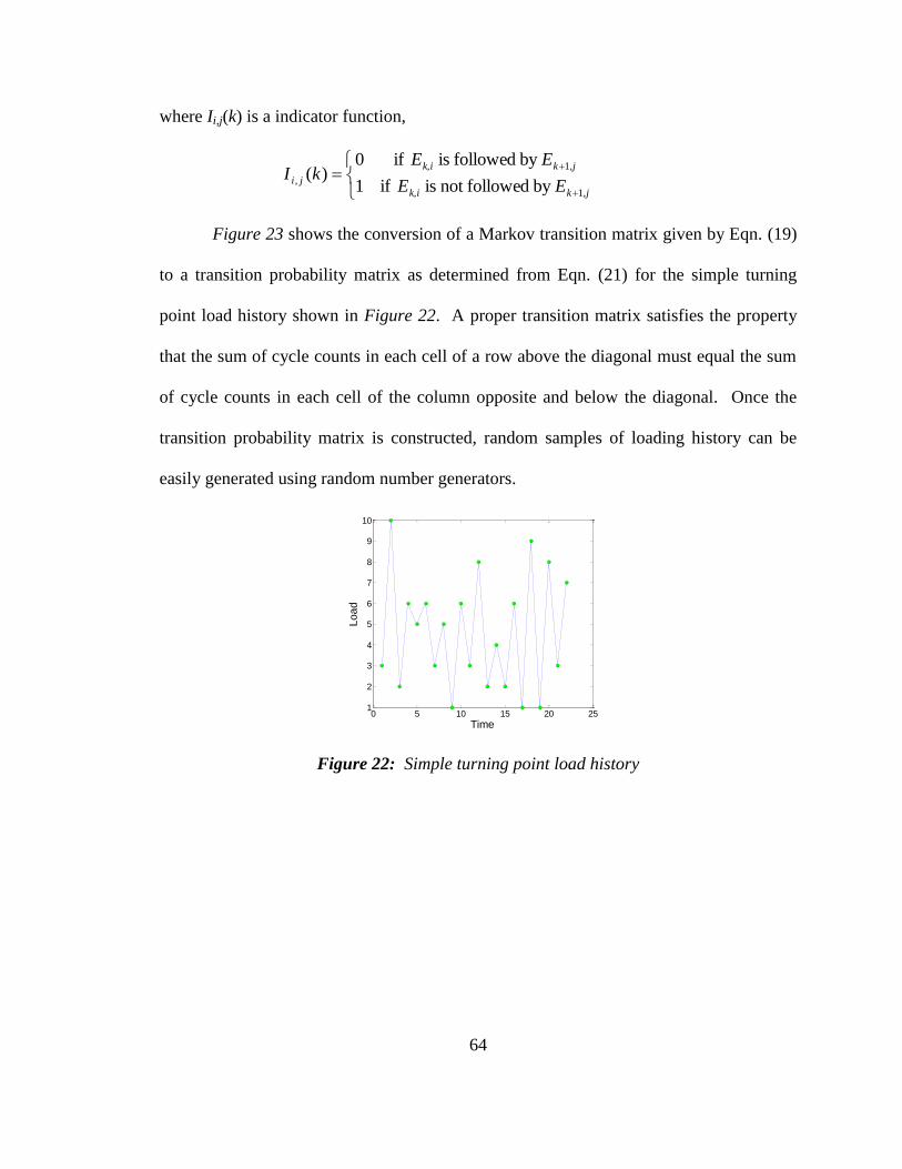
64
where Ii,j(k) is a indicator function,
,jkk,i
,jkk,i
ji EE
EEkI
1
1
, by followednot is if1
by followed is if0)(
Figure 23 shows the conversion of a Markov transition matrix given by Eqn. (19)
to a transition probability matrix as determined from Eqn. (21) for the simple turning
point load history shown in Figure 22. A proper transition matrix satisfies the property
that the sum of cycle counts in each cell of a row above the diagonal must equal the sum
of cycle counts in each cell of the column opposite and below the diagonal. Once the
transition probability matrix is constructed, random samples of loading history can be
easily generated using random number generators.
0 5 10 15 20 251
2
3
4
5
6
7
8
9
10
Time
Load
Figure 22: Simple turning point load history

65
a.) b.)
Figure 23: a.) Transition matrix b.) Transition probability matrix
Although measured time histories contain all of the information about the loading
history, it is difficult to obtain a clear understanding of the key characteristics of the data
when it is in this format, and makes load comparison between different histories virtually
impossible. To accurately characterize load values in a meaningful way, the content of a
measured signal must be summarized and quantified in an efficient and concise way.
Within this section, rainflow and Markov-based methods are presented as tools which
simplify the representation of fatigue loading within a complex, variable amplitude load
history. Additionally, methods are presented to more generally express the fatigue
loading content contained within a history by joint distribution functions and transition
probability matrices. Each of the load quantification methods contained within this
section is further developed within Chapter 3 to enable stochastic load simulation within
a probabilistic crack growth framework.
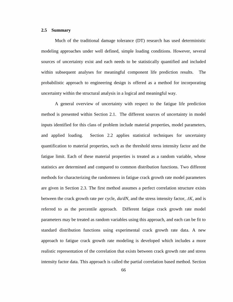
66
2.5 Summary
Much of the traditional damage tolerance (DT) research has used deterministic
modeling approaches under well defined, simple loading conditions. However, several
sources of uncertainty exist and each needs to be statistically quantified and included
within subsequent analyses for meaningful component life prediction results. The
probabilistic approach to engineering design is offered as a method for incorporating
uncertainty within the structural analysis in a logical and meaningful way.
A general overview of uncertainty with respect to the fatigue life prediction
method is presented within Section 2.1. The different sources of uncertainty in model
inputs identified for this class of problem include material properties, model parameters,
and applied loading. Section 2.2 applies statistical techniques for uncertainty
quantification to material properties, such as the threshold stress intensity factor and the
fatigue limit. Each of these material properties is treated as a random variable, whose
statistics are determined and compared to common distribution functions. Two different
methods for characterizing the randomness in fatigue crack growth rate model parameters
are given in Section 2.3. The first method assumes a perfect correlation structure exists
between the crack growth rate per cycle, da/dN, and the stress intensity factor, ΔK, and is
referred to as the percentile approach. Different fatigue crack growth rate model
parameters may be treated as random variables using this approach, and each can be fit to
standard distribution functions using experimental crack growth rate data. A new
approach to fatigue crack growth rate modeling is developed which includes a more
realistic representation of the correlation that exists between crack growth rate and stress
intensity factor data. This approach is called the partial correlation based method. Section

67
2.4 investigates two different methods for quantification and representation of variable
amplitude fatigue loading data. The rainflow cycle counting method can be used for this
purpose, and detailed methods of further fatigue relevant fatigue representation is
provided. The Markov based method is also presented within this section as an alternative
method for load characterization and quantification.
The different statistical methods presented within this chapter are given as useful
tools which can be used to characterize the randomness that exists in several of the model
inputs and/or model parameter values that are typically used within a damage tolerance
based fatigue life prediction analysis. Each method can be used individually to represent
a single random input, or collectively to more fully represent the overall stochastic nature
of inputs to the fatigue crack growth analysis. Chapter 3 develops a fatigue crack growth
modeling framework which enables systematic and efficient probabilistic fatigue life
prediction considering the uncertainty in model inputs identified and quantified within
this chapter.

68
CHAPTER III
PLANAR FATIGUE CRACK GROWTH MODELING
3.1 Introduction
This chapter explains the overall methodology that has been developed to model
fatigue crack propagation under multiaxial loading conditions using a planar fatigue
crack growth approach. The methodology has been developed with probabilistic analysis
in mind, where uncertainties at various levels of modeling can easily be included within
the overall framework.
For each deterministic analysis within the Monte Carlo scheme, input variables
such as initial crack size, crack shape, and crack growth model parameter values are
sampled from their given distributions. A stochastic load history is simulated based on
fatigue relevant statistics determined from a representative load history. A cycle by cycle
approach is adopted where a stress intensity factor is evaluated for the current loading
cycle and crack configuration using a trained surrogate model. Crack growth rate
calculations can be performed along the crack front using a stochastic fatigue crack
growth rate model and the crack front can be appropriately extended. Cyclic crack growth
analysis is repeated using the same load history from the initial crack size until a user
defined critical crack size is reached, at which time the results are stored and the
procedure is repeated for the next realization of input variables. After many simulations
are completed, it is possible to extract probabilistic information such as the probability
distribution of the crack size at any given time, t, or, conversely the probability
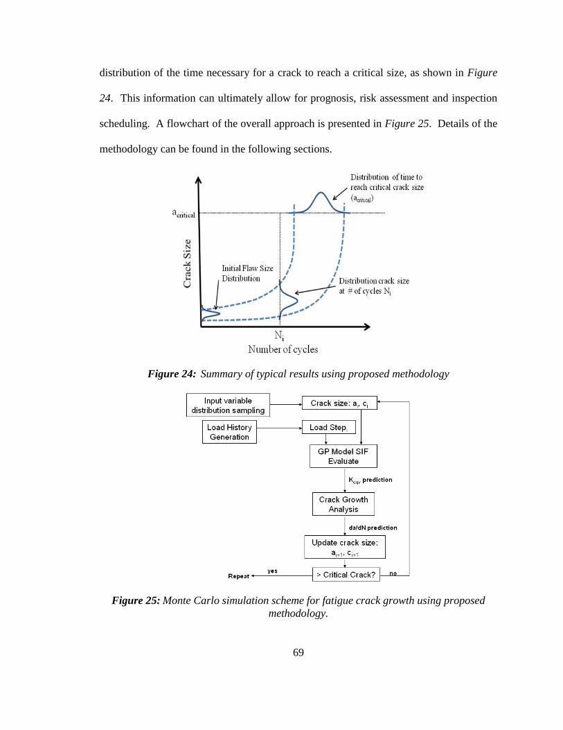
69
distribution of the time necessary for a crack to reach a critical size, as shown in Figure
24. This information can ultimately allow for prognosis, risk assessment and inspection
scheduling. A flowchart of the overall approach is presented in Figure 25. Details of the
methodology can be found in the following sections.
Figure 24: Summary of typical results using proposed methodology
Figure 25: Monte Carlo simulation scheme for fatigue crack growth using proposed
methodology.

70
3.2 Initial Flaw Size & Location
The first step in performing a damage tolerance analysis, in which an initial flaw
is assumed to be contained within the component of interest, is to fully characterize the
flaw which is to be modeled. For this research, only surface crack configurations will be
considered. The surface crack configuration is controlled by two parameters, namely;
crack length (2c) and aspect ratio. Here, aspect ratio is defined as the ratio of half the
crack length over the crack depth (c/a) as shown in Figure 26.
Figure 26: Semi-Elliptical Crack showing crack length (2c) and depth (a)
definitions
It is clear that different locations within the component will be subjected to
different stresses based on the type of applied loading and the geometry of the component
of interest. Since fatigue crack propagation depends not only on the crack size and shape,
but also on the stress concentration at the crack front, cracks with the same initial
configuration but at different locations within the component will have different
propagation rates, and thus, will cause different component life predictions. Based on
this information, the most critical location is that which will cause the crack to grow the
fastest, causing the component to break in the least amount of time. MIL-A-83444
handbook [76] states that “the analyses shall assume the presence of flaws placed in the

71
most unfavorable location and orientation with respect to the applied stresses and
material properties.”
In order to identify this critical location, a preliminary stress analysis of the
uncracked component can be completed. Loading conditions similar to those expected
in-service are applied to the component and the stress field can then be analyzed to
identify the region with the highest stress concentration. By performing this analysis on
an uncracked component, the critical location can be identified and a crack can be
inserted in the structural model such that it is perpendicular to the maximum principal
stress direction at that location.
Figure 27: Plot of typical stress profile within rotorcraft mast component under applied
mixed mode loading
Ideally, fatigue life prediction could be performed starting from an actual, as-
manufactured initial flaw size, accounting for actual voids, non-metallic inclusions, or
surface scratches contained within the material. However, determining the true
distribution of initial flaw sizes within an as-manufactured part is, often times, difficult to
accomplish due to inadequate resources and/or the limited capability of non-destructive
evaluation (NDE) techniques for reliably detecting small crack sizes. If the actual initial
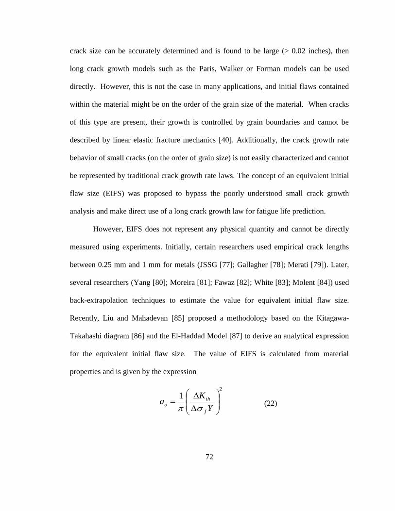
72
crack size can be accurately determined and is found to be large (> 0.02 inches), then
long crack growth models such as the Paris, Walker or Forman models can be used
directly. However, this is not the case in many applications, and initial flaws contained
within the material might be on the order of the grain size of the material. When cracks
of this type are present, their growth is controlled by grain boundaries and cannot be
described by linear elastic fracture mechanics [40]. Additionally, the crack growth rate
behavior of small cracks (on the order of grain size) is not easily characterized and cannot
be represented by traditional crack growth rate laws. The concept of an equivalent initial
flaw size (EIFS) was proposed to bypass the poorly understood small crack growth
analysis and make direct use of a long crack growth law for fatigue life prediction.
However, EIFS does not represent any physical quantity and cannot be directly
measured using experiments. Initially, certain researchers used empirical crack lengths
between 0.25 mm and 1 mm for metals (JSSG [77]; Gallagher [78]; Merati [79]). Later,
several researchers (Yang [80]; Moreira [81]; Fawaz [82]; White [83]; Molent [84]) used
back-extrapolation techniques to estimate the value for equivalent initial flaw size.
Recently, Liu and Mahadevan [85] proposed a methodology based on the Kitagawa-
Takahashi diagram [86] and the El-Haddad Model [87] to derive an analytical expression
for the equivalent initial flaw size. The value of EIFS is calculated from material
properties and is given by the expression
2
1
Y
Ka
f
tho
(22)

73
where ao is the EIFS, ΔKth is the threshold stress intensity factor range, Δσf is the fatigue
limit, and Y is the geometry correction factor.
The current research work uses Eqn. (22) to calculate the statistics of EIFS by
using the probability distribution functions of the threshold stress intensity factor and
fatigue limit. The distribution functions of these material properties were determined
within Chapter III of this work, considering both natural variability in experimental data
and data uncertainty due to sparse data. By using this physics based approach, the
analytical expression in Eqn. (22) can be used to determine a distribution of the EIFS.
The distribution of EIFS for 7075-T6 Aluminum alloy is included within Figure 28 and
can be sampled within the subsequent probabilistic crack growth analysis. Since both the
threshold stress intensity factor and the fatigue limit have been determined to fit the
lognormal distribution function for this material, the EIFS will also be a lognormal
variable. However, this is not a necessary condition, and the distribution of EIFS can be
easily determined (despite the distribution functions of ΔKth and σf, through simple
sampling techniques.
0.01 0.015 0.02 0.025 0.03 0.035 0.040
20
40
60
80
100
120
Crack Length (in)
Density
Calculated EIFS Values
Lognormal Dist.
Figure 28: 10,000 calculated EIFS value and best fit lognormal distribution function for
Aluminum Alloy 7075-T6

74
3.3 Component Stress Analysis
For standard fatigue specimen subjected to uniaxial loading conditions, handbook
solutions for stress intensity factors are available [88]. For structures having complicated
geometry or complex multi-axial loading conditions, a handbook solution for the stress
intensity factor, ΔK, may not be available and finite element analysis (FEA) may be
required. Although the computational expense can be significant for high fidelity
models, FEA analysis is still necessary in some capacity to determine the stress state at
the crack tip, and must be performed for complex geometry and loading conditions.
A two level approach is adopted for finite element analysis within this work,
using a global model and a submodel. The crack region represents a relatively small
volume of material that lies within the larger volume of the overall component and is
constructed within a submodel for better computational efficiency and accuracy. The
submodel method is a technique to obtain a more accurate numerical value for the
specific region in the analyzed model with high efficiency, and is sometimes referred to
as the cut-boundary displacement method or the specified boundary displacement
method. The boundary of the sub model represents a cut through the coarse model, where
displacement boundary conditions are enforced.
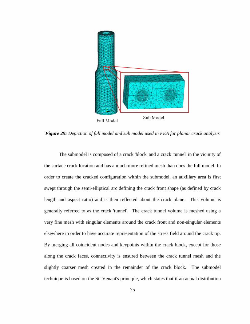
75
Figure 29: Depiction of full model and sub model used in FEA for planar crack analysis
The submodel is composed of a crack 'block' and a crack 'tunnel' in the vicinity of
the surface crack location and has a much more refined mesh than does the full model. In
order to create the cracked configuration within the submodel, an auxiliary area is first
swept through the semi-elliptical arc defining the crack front shape (as defined by crack
length and aspect ratio) and is then reflected about the crack plane. This volume is
generally referred to as the crack 'tunnel'. The crack tunnel volume is meshed using a
very fine mesh with singular elements around the crack front and non-singular elements
elsewhere in order to have accurate representation of the stress field around the crack tip.
By merging all coincident nodes and keypoints within the crack block, except for those
along the crack faces, connectivity is ensured between the crack tunnel mesh and the
slightly coarser mesh created in the remainder of the crack block. The submodel
technique is based on the St. Venant's principle, which states that if an actual distribution
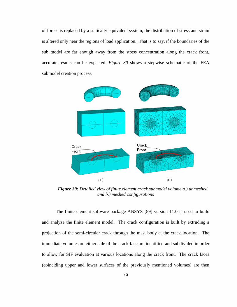
76
of forces is replaced by a statically equivalent system, the distribution of stress and strain
is altered only near the regions of load application. That is to say, if the boundaries of the
sub model are far enough away from the stress concentration along the crack front,
accurate results can be expected. Figure 30 shows a stepwise schematic of the FEA
submodel creation process.
Figure 30: Detailed view of finite element crack submodel volume a.) unmeshed
and b.) meshed configurations
The finite element software package ANSYS [89] version 11.0 is used to build
and analyze the finite element model. The crack configuration is built by extruding a
projection of the semi-circular crack through the mast body at the crack location. The
immediate volumes on either side of the crack face are identified and subdivided in order
to allow for SIF evaluation at various locations along the crack front. The crack faces
(coinciding upper and lower surfaces of the previously mentioned volumes) are then

77
modeled as surface to surface contact elements (CONTACT174 and TARGET170
elements) in order to prevent the surface penetration of the crack's upper and lower
surfaces. The augmented Lagrangian method is the algorithm used for contact
simulation. Additionally, friction effect is included in the material properties of the
contact element, in which a Coulomb friction model is used. This model defines an
equivalent shear stress which is proportional to the contact pressure and the friction
coefficient. Friction coefficients between two crack faces are difficult to measure and are
generally assumed to vary between 0 and 0.5 [90]. The friction coefficient, μ, used within
this study is assumed to be a deterministic quantity and taken to be equal to 0.1.
Since the primary quantity of interest is the stress intensity factor at the crack tip,
the volume along the crack front is subdivided into many smaller blocks, which allows
for better mesh control and enables SIF evaluation at various locations along the crack
front. The ¼ node displacement method proposed by Henshell and Shaw [91] and
Barsoum [92] has been commonly used to enable the square root singularity of stresses
and strains at the crack tip to be modeled accurately by shifting the mid-point nodes to
the quarter-point locations in the region around the crack front. Stress intensity factors at
the surface and depth locations are calculated and are used within fatigue crack growth
models for crack extension calculations, allowing for initial semi-circular surface cracks
to develop into semi-elliptical cracks over time.

78
3.4 Equivalent Mixed-Mode Stress Intensity Factor
Many mechanical and structural components are subjected to some combination
of tension, bending, bearing, and torsion, in which some combination of mode I, mode II,
and mode III loading conditions exist (e.g. mast in rotorcraft, railroad wheels, turbine
blades, shafts of automobiles [93,94,95]), however only limited research has been
reported in the literature. Carpinteri [96,97] analyzed hollow pipes with elliptical surface
cracks under bending moment and axial loading separately. Fonte [98] applied bending
moment to a round bar with a circumferential elliptical crack and validated his results
with previously published results in the literature, followed by an analysis of torsion
loading only. He then applied both bending moment and torsion loading, and checked the
superposition principle. Results showed that the application of bending moment induced
only Mode I at the crack front, whereas the application of torsion induced all three modes
of loading at the crack front.
The stress intensity factor is the primary parameter used for fatigue crack growth
rate prediction and is typically used with many commonly used fatigue crack growth rate
models including the Walker [7], Forman [6], and Forman-Newman-de Koning [99]
models.
Several parameters have been used to correlate fatigue crack growth rates under
mixed mode conditions. These include equivalent stress intensity factors, equivalent
strain intensity factors, strain energy density, and the J-integral [69]. These methods
develop different expressions for an equivalent stress intensity factor range, ΔKeqv, which
has been used to obtain the crack growth rate for mixed-mode loading condition in a
Paris-type equation [69].

79
This research uses a characteristic plane-based model for multi-axial fatigue
damage modeling proposed by Liu and Mahadevan [100,101], which is applicable to a
wide range of metallic materials and has been validated using multiaxial fatigue
experimental data. The characteristic plane-based model enables the calculation of an
equivalent mixed mode stress intensity factor which can be used for mixed mode fatigue
crack propagation and life prediction calculations. A detailed derivation and explanation
of the model can be found in Liu and Mahadevan [101] and the concepts will only be
briefly summarized within this section as necessary for basic understanding of the
methodology.
The characteristic plane-based approach seeks to reduce the dimension of the
multiaxial fatigue problem by considering the stress components on a given plane, the
characteristic plane, so that traditional crack growth models can be implemented, and in
doing so, also reduces the necessary computational effort [101]. The formula under
general mixed mode I+II+III loading is derived as
BK
kA
K
k
K
k
K
k
thI
H
thIII
III
thII
II
thI
I
2
,
2
,
2
,
2
,
(23)
where kI, kII, and kIII are the mode I, II and III loading factors with the same unit of stress
intensity factors, and KI,th, KII,th, and KIII,thI are the fatigue crack threshold values,
respectively. kH is the hydrostatic stress related term, and A and B are material parameters
which can be determined by tension and shear fatigue limits. The characteristic plane for
a given material is determined through minimizing the contribution of the hydrostatic
stress amplitude to zero.

80
Table 3: Material Properties for fatigue damage accumulation using characteristic plane
approach
Material
Property
11
1
f
ts 1
1
1
f
ts
22
222
4/152
4/153/1442)2cos(
ss
sss
0
A A=0 19 2 sA
B 2
1222 2sin2cos sB
sA
Following the derivation outlined by Liu [101], the equivalent mixed mode stress
intensity factor using the characteristic plane approach can be expressed as
dN
daf
s
kA
s
k
s
kk
BK
H
IIIIIIeqvmixed
222
2
,
1 (24)
The equivalent uniaxial stress intensity factor, eqvmixedK , , could be used within any
available fatigue crack growth model by a simple substitution of the mode I stress
intensity factor, ΔKI, used in the original formulation with the newly defined parameter
ΔKmixed, eqv.

81
3.5 Surrogate Model Development
The previous two sections within this chapter presented methods for the
multiaxial stress analysis of a fatigue critical component using FEA, and a stress intensity
factor dimension reduction technique for calculation of equivalent, uniaxial stress
intensity factor. Within a damage tolerance analysis, where initial cracks are grown
incrementally until they reach a critical crack size, each of these steps is necessary for
each crack growth increment within the analysis, requiring substantial computational
effort. The computational expense associated with the stress intensity factor calculation
typically results from the need to implement an expensive finite element code for the
current crack size and loading conditions. In order to implement this type of analysis
within a probabilistic framework, where many full simulations are necessary, a more
efficient method for determining the stress intensity factor at the ever evolving crack
front must be developed.
Response surface methodology can be used in place of expensive finite element
models for iterative fatigue analysis to reduce the computational effort needed to
calculate the stress intensity factor at the crack tip. A response surface approximation is
constructed to approximately capture the relationship between the input variables (crack
length, location, and load values) and the output variables (stress intensity factors), using
only a few sample points within the design space. Instead of using a finite element model
to determine the stress intensity factors at every load step within every simulation, the
model is analyzed for a small number of crack configurations and loading conditions to
"train" a surrogate model to an acceptable degree of accuracy. Once trained, the surrogate
model is used in place of the full finite element model. By developing an accurate

82
surrogate model and drastically reducing the computational effort needed at load cycle
within the analysis, it is possible to use a Monte Carlo simulation technique for
component reliability assessment.
Many different types of surrogate models have been developed and reported
within the literature including: locally weighted polynomial regression, quadratic
response surface regression (QREG), random forest regression (RF), gradient boosting
machine (GBM), multivariate adaptive regression splines (MARS), support vector and
relevance vector regression, neural networks and Gaussian process models [102,103]. An
initial study of several methods was performed to evaluate the relative performance of
each as applied to the FEA/stress analysis problem. Results from the study are included
in Table 4, and revealed the Gaussian process model to have an overall better
performance when compared to the other methods with the same level of training. The
Gaussian process model will be implemented within this research due to its flexibility
and relative performance when compared with other available methods.
Table 4: Comparison of surrogate model performance for stress analysis application
Surrogate Model Sum of Squares of Errors
Polynomial Chaos Expansion 57.7 units
Support Vector Regression 55.1 units
Relevance Vector Regression 54.9 units
Gaussian Process Interpolation 50.3 units
Gaussian process (GP) modeling (which is in most cases equivalent to the family
of methods which go by the name of “Kriging” predictors) is a powerful technique based
on spatial statistics for interpolating data. Gaussian process models are increasingly being

83
used as surrogates to expensive computer simulations for the purposes of optimization
and uncertainty propagation [104,105], and will be investigated within this paper as
method to improve computational efficiency by replacing the expensive stress intensity
factor calculation.
The basic idea of the GP model is that the response values, Y, are modeled as a
group of multivariate normal random variables, with a defined mean and covariance
function. A recently developed greedy point selection technique can be used to select
training points for the GP model to build up the response surface to a desired level of
accuracy [106]. The benefits of GP modeling is that the method requires only a small
number of sample points (usually 30 or less), and is capable of capturing highly nonlinear
relationships that exist between input and output variables without the need for an
explicit functional form. Additionally, Gaussian process models can be used to fit
virtually any functional form and provide a direct estimate of the uncertainty associated
with all predictions in terms of model variance.
In order to accurately capture the functional relationship between input and output
quantities, the Gaussian Process model must be "trained" using a set of observed inputs
and outputs. The Greedy Point algorithm [106] can be used to identify which points
within the design space would be the most advantageous to use as training points. As
mentioned previously, the variance associated with model predictions is available as a
result of the Gaussian Process formulation. The Greedy Point algorithm uses this
information to identify the set of input variable values (design space location) which
correspond to the largest variance in the design space, and selects the next training point
to be at that location, thus improving the model by minimizing the model prediction

84
error. By repeating the Greedy Point algorithm iteratively, training points can be
identified that minimize the variance of the surrogate model until a sufficiently accurate
model is generated, say within 1% or 5% of FEA. This training point selection method
eliminates the subjectivity associated with typical design of experiments methods which
use a pre-determined fixed set of training points, and ensures that the identified training
points are adding the most value (accuracy) to the surrogate model per additional full
simulation run.
Suppose that there are n training points, x1, x2, x3 … xn of a d-dimensional input
variable (the input variables being the crack size and loading conditions here), yielding
the resultant observed random vector Y(x1), Y(x2), Y(x3) … Y(xn). R is the n x n matrix of
correlations among the training points. Under the assumption that the parameters
governing both the trend function (fT(xi) at each training point) and the covariance (λ) are
known, the conditional expected value of the process at an untested location x* is
calculated as in Eqn. (25) and Eqn. (26) respectively.
)(| 1**** FYRxrxfxYEY TT
(25)
rRrxYVar T
Y
1* 1|*
(26)
In Eqn. (25) and Eqn. (26), F is a matrix with rows i
T xf , r is the vector of
correlations between x* and each of the training points, β represents the coefficients of
the regression trend. McFarland [106] discusses the implementation of this method in
detail.

85
Figure 31: Schematic of GP training process using iterative greedy point algorithm
The GP surrogate modeling technique offers several advantages which prove
useful. The first is that the GP modeling approach is a non-parametric technique,
meaning that assumptions about the functional form (linear, quadratic, power, etc.) are
not necessary. The framework is flexible and can capture linear and non-linear
relationships that exist within the design space. A second significant attribute of the GP
modeling approach is that the method has the ability to provide a direct representation of
the uncertainty associated with its interpolative approximation [106]. This uncertainty
representation has been shown to provide usefulness in improving both the efficiency of
optimization [107] and reliability estimation [108].

86
3.6 Variable Amplitude Load Generation
By reducing the complex load history into its elementary load cycles and storing
the information in a rainflow or Markov transition matrix representation, significant
advantages are gained in terms of ease of quantification of the measured load spectrum.
However, the sequence of the loading is lost. Loading sequence is of importance since it
is well known that amplitude changes in fatigue loading conditions can result in
significant retardation or acceleration of fatigue crack growth rates [109]. This section
address this issue and presents stochastic regeneration techniques that can be used to
produce multiple realizations of load histories that contain the same fatigue loading
characteristics as the original representative load history
It is well known that crack growth can be significantly affected by prior events in
the load history [69]. There is vast literature showing that tensile overloads can cause
retardation or arrest in fatigue crack growth and compressive overloads can also have
significant effects on the rate of subsequent crack propagation [110]. Ignoring such
effects can lead to significant error in fatigue life estimation. Therefore, it is necessary to
incorporate a methodology that uses the sequence of loadings in the life prediction.
Several different reconstruction techniques have been reported within the literature
including traditional power spectral density techniques [111], Markov simulations [72],
rainflow [112], among others. It is proposed that by utilizing stochastic reconstruction
methods in combination with the load quantification results developed in Chapter 2, it is
possible to generate multiple realizations of the fatigue content to represent several
different load sequences.

87
Rainflow Stochastic Load Reconstruction
The basic objective of the stochastic rainflow reconstruction algorithm is to create
a systematic method to reconstruct a load history given a rainflow matrix and its residual.
Dreβler [113] presents an algorithm for reconstruction and approaches the problem so
that an optimal randomization of the reconstructed series is attained. Rainflow
reconstructions are based on the idea of extracting cycles from the rainflow matrix and
placing them in valid locations in the history under construction. Several rules exist to
ensure that cycles are inserted within the residual in such a way as to yield a similar
rainflow matrix as the original signal.
Reconstruction is performed in such a way that fatigue cycles are reinserted into
the residual in order of their respective amplitudes, with largest amplitudes inserted first.
Randomness is introduced into the load reconstruction process by first identifying all of
the „allowable‟ locations for reinsertion of the current load cycle under consideration, and
then sampling from a distribution function to randomly select the insertion location. After
insertion, the cycle is deleted from the rainflow matrix, and the cycle with the next largest
amplitude is considered. This process is repeated until the rainflow matrix is empty and
all cycles have been reinserted into the residual. Numerous random sequences can be
generated in this manner, and used to quantify the effect of load sequence on fatigue life
prediction.
Assuming a fully populated rainflow matrix is available, an algorithm can be
implemented to reproduce a new turning point sequence, whose rainflow counting result
is identical to that obtained from the original spectrum. Due to the fact that inserting a
turning point pair (max-min or min-max pair) does not affect the possibility of inserting
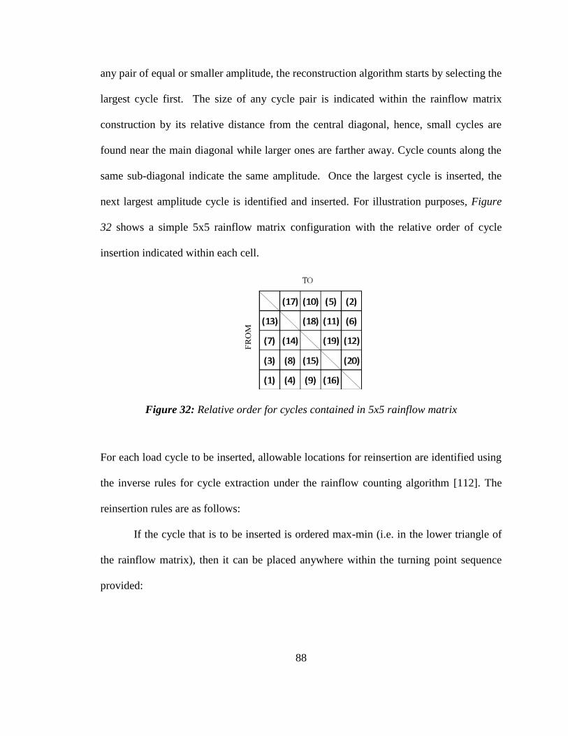
88
any pair of equal or smaller amplitude, the reconstruction algorithm starts by selecting the
largest cycle first. The size of any cycle pair is indicated within the rainflow matrix
construction by its relative distance from the central diagonal, hence, small cycles are
found near the main diagonal while larger ones are farther away. Cycle counts along the
same sub-diagonal indicate the same amplitude. Once the largest cycle is inserted, the
next largest amplitude cycle is identified and inserted. For illustration purposes, Figure
32 shows a simple 5x5 rainflow matrix configuration with the relative order of cycle
insertion indicated within each cell.
Figure 32: Relative order for cycles contained in 5x5 rainflow matrix
For each load cycle to be inserted, allowable locations for reinsertion are identified using
the inverse rules for cycle extraction under the rainflow counting algorithm [112]. The
reinsertion rules are as follows:
If the cycle that is to be inserted is ordered max-min (i.e. in the lower triangle of
the rainflow matrix), then it can be placed anywhere within the turning point sequence
provided:

89
1. If the receiving cycle is ordered min-max (row # < column #), then receiving
row must be less than or equal to the inserting column, and the receiving
column must be greater than or equal to the inserting row
2. If the receiving cycle is ordered max-min (row # > column #), then the
receiving row must be greater than or equal to the inserting row, and the
receiving column must be less than or equal to the inserting column
Similarly, if the cycle that is to be inserted is ordered min-max (i.e. in the upper
triangle of the rainflow matrix), then it can be placed anywhere within the turning point
sequence provided:
3. If the receiving cycle is ordered max-min (row # > column #), then receiving
row must be greater than or equal to the inserting column, and the receiving
column must be less than or equal to the inserting row
4. If the receiving cycle is ordered min-max (row # < column #), then the
receiving row must be less than or equal to the inserting row, and the
receiving column must be greater than or equal to the inserting column
Additionally, the reconstruction must alternate between local minimum and maximum
values, i.e. maintain a turning point sequence. These rules ensure that the inserting cycle
is smaller in amplitude than the receiving cycle and that all cycles within the rainflow
matrix are guaranteed to have at least one feasible insertion location. As a result, the
newly constructed load history is guaranteed to have the identical rainflow count as that
obtained from the original history.

90
Markov Chain Stochastic Load Reconstruction
Stochastic load reconstruction using the Markov chain method is simple and
straightforward. The reconstruction technique utilizes both the transition probabilities
contained within the Markov transition probability matrix as well as random number
generators. First, the transition probabilities contained within each row within the upper
diagonal of the transition probability matrix given in Eqn. (21) are converted to
cumulative density functions. Since the Markov transition matrix is composed of n
discrete load levels (as detailed in Section 2.4 and shown in Eqn. (19)), the cumulative
distribution function for any load transition from level i can be calculated by the
summation of the individual transition probabilities. To maintain the turning point
sequence, i.e. maintain minimummaximumminimum order, the cumulative discrete
distribution function can be calculated as:
jip
jip
xXPxFi
j
ji
n
ij
ji
1
1
,
1
,
)()( (27)
Assume an initial load minimum at state i is known. Stochastic simulation of the
subsequent load state j can be performed through the following steps
1. Calculate the CMF along row i using the transition probability information
above the main diagonal
2. Generate a uniform random number, x, within the bounds [0,1]
3. Compare the random number, x, to the CMF contained within each level j
4. Select the new load level j for which x is ≥ CMFj-1 and ≤ CMFj and add to
turning point history

91
5. Set i = j and repeat steps 14
For the purpose of illustrating the applicability of the reconstruction methods
outlined within this section, the scaled helicopter combat maneuver loading history as
presented in Khosrovaneh [114] and shown in Figure 33, is presented with numerical
reconstruction using both the rainflow and Markov chain stochastic methods. The
reconstructed load histories using the rainflow technique are seen in Figure 34 and
closely resemble the original load sequence by retaining major sequence trends and load
magnitudes.
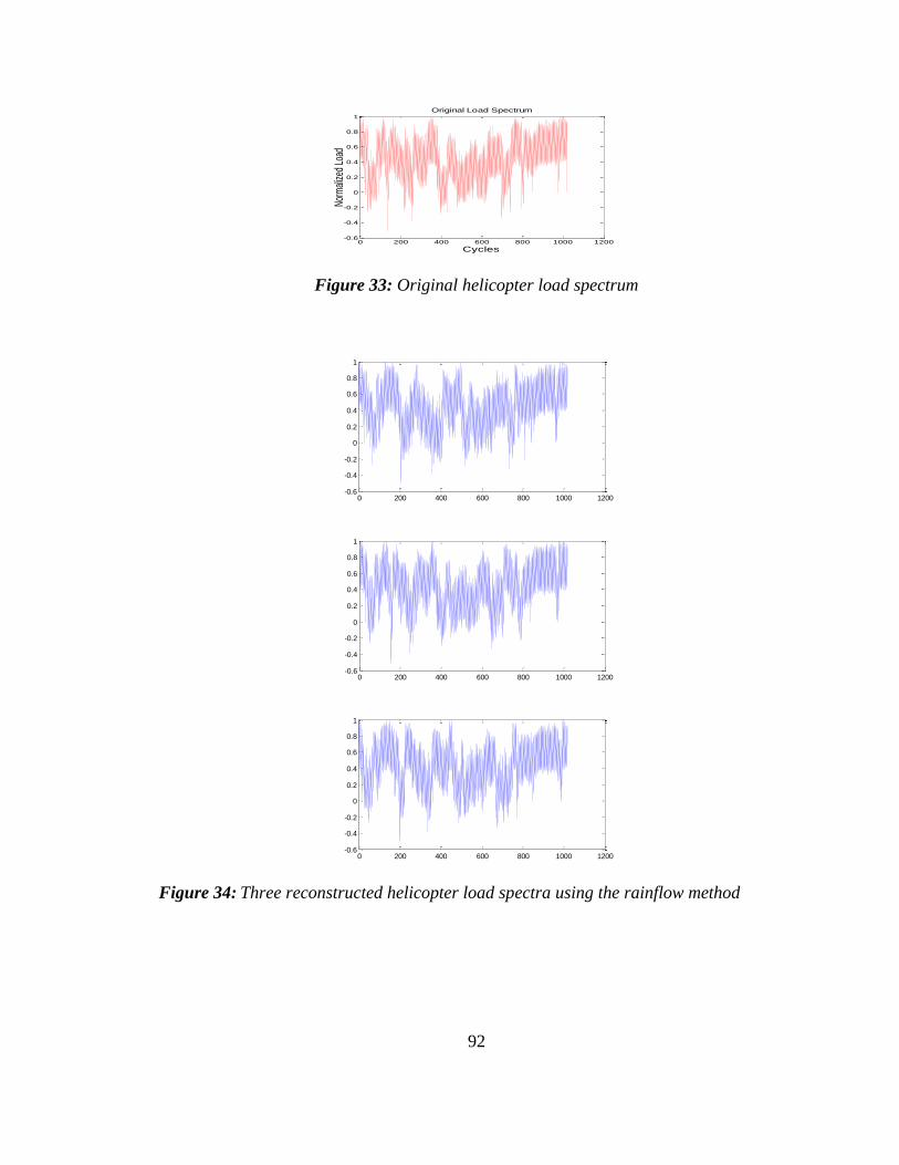
92
0 200 400 600 800 1000 1200-0.6
-0.4
-0.2
0
0.2
0.4
0.6
0.8
1Original Load Spectrum
Cycles
Nor
mal
ized
Loa
d
Figure 33: Original helicopter load spectrum
0 200 400 600 800 1000 1200-0.6
-0.4
-0.2
0
0.2
0.4
0.6
0.8
1
0 200 400 600 800 1000 1200-0.6
-0.4
-0.2
0
0.2
0.4
0.6
0.8
1
0 200 400 600 800 1000 1200-0.6
-0.4
-0.2
0
0.2
0.4
0.6
0.8
1
Figure 34: Three reconstructed helicopter load spectra using the rainflow method

93
Similarly, load reconstruction can be performed for the same helicopter spectrum
using the Markov method. Two simulated load histories obtained using this method can
be seen in Figure 35.
0 200 400 600 800 1000 1200-0.4
-0.2
0
0.2
0.4
0.6
0.8
1
0 200 400 600 800 1000 1200-0.4
-0.2
0
0.2
0.4
0.6
0.8
1
Figure 35: Reconstructed helicopter load spectra using the Markov transition method
As can be seen within Figure 35, the Markov method appears to be capable of
stochastic reconstruction of variable amplitude load histories, however, the newly
constructed loads appear to be slightly more randomly structured than those histories
constructed using the rainflow methods. This is evident by looking at the major trend
contained within the original load history (Figure 33) between approximately the 400 and
1000 cycle. An overall positive trend is observed in both the original spectrum as well as
the reconstructed rainflow spectra. Both of the reconstructions using the Markov method
failure to capture this major trend, and appear to have a more stationary random behavior
than the original data set. However, the simulated load history using the Markov method
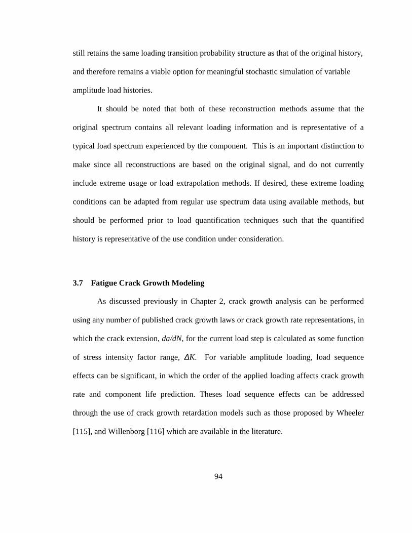
94
still retains the same loading transition probability structure as that of the original history,
and therefore remains a viable option for meaningful stochastic simulation of variable
amplitude load histories.
It should be noted that both of these reconstruction methods assume that the
original spectrum contains all relevant loading information and is representative of a
typical load spectrum experienced by the component. This is an important distinction to
make since all reconstructions are based on the original signal, and do not currently
include extreme usage or load extrapolation methods. If desired, these extreme loading
conditions can be adapted from regular use spectrum data using available methods, but
should be performed prior to load quantification techniques such that the quantified
history is representative of the use condition under consideration.
3.7 Fatigue Crack Growth Modeling
As discussed previously in Chapter 2, crack growth analysis can be performed
using any number of published crack growth laws or crack growth rate representations, in
which the crack extension, da/dN, for the current load step is calculated as some function
of stress intensity factor range, ΔK. For variable amplitude loading, load sequence
effects can be significant, in which the order of the applied loading affects crack growth
rate and component life prediction. Theses load sequence effects can be addressed
through the use of crack growth retardation models such as those proposed by Wheeler
[115], and Willenborg [116] which are available in the literature.

95
Within this research, the fatigue crack growth rate is modeled using the modified
Paris fatigue crack growth law, as initially presented in Eqn. (9), along with Wheeler‟s
crack retardation model to include load sequence effects given by Eqn. (28).
p
thmr
K
KKC
dN
da
1)( (28)
In Eqn. (28), υr refers to the retardation parameter, and is equal to unity if ai + rp,i > aOL
+ rp,OL where aOL is the crack length at which the overload is applied, ai is the current
crack length, rp,OL is the size of the plastic zone produced by the overload at aOL, and rp,i
is the size of the plastic zone produced at the current crack length ai. Else, υr is
calculated as shown in Eqn. (29)
iOLpOL
pir
ara
r
,
(29)
where λ is the curve fitting parameter for the original Wheeler model termed the shaping
exponent. Sheu et al. [117] and Song et al. [118] observed that crack growth retardation
actually takes place within an effective plastic zone. Hence the size of the plastic zone
can be calculated in terms of the applied stress intensity factor (K) and yield strength (σ)
as:
2
Krp
(30)
In Eqn. (30), α is referred to as the effective plastic zone size constant which is
calculated experimentally [119]. Immediately following the overload, the retardation
parameter υr < 1. As the crack growths through the overload plastic zone, υ
r increases
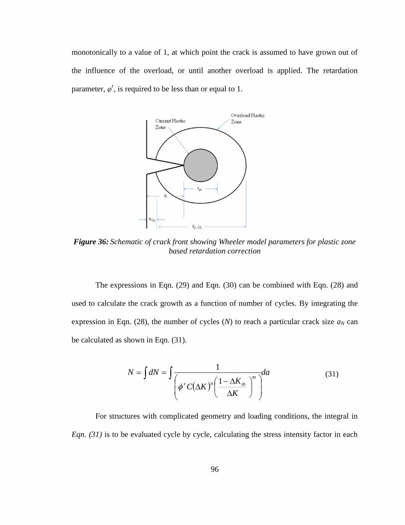
96
monotonically to a value of 1, at which point the crack is assumed to have grown out of
the influence of the overload, or until another overload is applied. The retardation
parameter, υr, is required to be less than or equal to 1.
Figure 36: Schematic of crack front showing Wheeler model parameters for plastic zone
based retardation correction
The expressions in Eqn. (29) and Eqn. (30) can be combined with Eqn. (28) and
used to calculate the crack growth as a function of number of cycles. By integrating the
expression in Eqn. (28), the number of cycles (N) to reach a particular crack size aN can
be calculated as shown in Eqn. (31).
da
K
KKC
dNNm
thnr
1
1
(31)
For structures with complicated geometry and loading conditions, the integral in
Eqn. (31) is to be evaluated cycle by cycle, calculating the stress intensity factor in each

97
cycle of the crack growth analysis. Since the stress intensity factor varies along the
periphery of the crack front, so too will the predicted crack growth rate.
Within this study, the stress intensity factor for a planar crack will be calculated at
two points along the crack front; at the crack tip at the surface and at the crack tip at the
depth (semi-major and semi-minor axis locations). This modeling approach allows for
initially semi-circular cracks to develop into semi-elliptical cracks. For the planar crack
growth analysis procedure, the crack growth direction remains in-plane with the initial
crack orientation.
3.8 Summary
This chapter presented various methods which, when used in combination, enable
efficient probabilistic fatigue crack growth analysis of planar, semi-elliptical surface
cracks under multiaxial, variable amplitude loading conditions. Several different topics
were covered including the statistical representation of the initial flaw size using EIFS
concepts, efficient stress intensity factor determination using FEA and surrogate
modeling techniques, stochastic load representation, and crack growth modeling.
The methodology incorporates some key features which enable efficient
probabilistic fatigue crack growth analysis considering multiple sources of uncertainty.
One key improvement over previous research includes the statistical representation of the
initial crack size by sampling the statistical distributions of material properties (threshold
stress intensity factor and fatigue limit). The EIFS concept enables the use of well
defined, long crack growth modeling which overcomes the limitations associated with

98
small crack growth modeling and provides a physics-based approach for EIFS
formulation. Another key contribution is the development of a new modeling construct
for fatigue crack growth analysis which allows for accurate and efficient component
stress analysis and stress intensity factor determination using finite element models and
surrogate modeling techniques. The Gaussian process interpolation response surface is
used to replace the computationally expensive hierarchical finite element analysis and
provides quick and accurate stress intensity factor solutions for any combination of crack
sizes, shapes, and loading parameters that are within the design space, without the need
for constant remeshing at the crack front. A new method is implemented to determine
which input variable combinations should be evaluated within the FEA by identifying
regions within the design space which are not well characterized by the current model.
Two methods for variable amplitude stochastic load reconstruction are also developed for
use within the cyclic fatigue crack growth analysis in order to consider the uncertainty in
load sequence which may result from different use conditions. Both methods appear to
be capable of regenerating stochastic load realizations based on the statistical
characterization of the original load sequence.
The uncertainty quantification techniques presented in Chapter 2 can be used with
the proposed framework developed in this chapter by implementing a sampling based
strategy within a Monte Carlo framework. Chapter 4 will investigate the additional
uncertainties introduced by the numerical methods introduced in this chapter and will
develop suitable methods for quantifying and incorporating these additional uncertainties
within the overall component fatigue life prediction.

99
CHAPTER IV
UNCERTAINTY QUANTIFICATION IN PLANAR CRACK GROWTH
ANALYSIS
4.1 Introduction
As our dependence upon both numerical and finite element models increases for
stress intensity factor calculation and fatigue life estimation, it is important that we
acknowledge that modeling error exists in each model used. Contained within each
model, be it numerical or some other form, simplifications and assumptions are made in
order to enable analysis of a real system by means of the model. Therefore, some errors
will exist in the model predictions when compared with reality. By improving the
resolution or complexity of the models and limiting the number of simplifications and
assumptions contained within them, it is possible to reduce model error, but at the
expense of computational efficiency.
The use of various numerical simulation models for the analysis of complex
system performance incorporates many approximations and assumptions which result in
errors in model predictions. Before higher system level analysis can be performed, it is
first necessary to evaluate the accuracy of the simulation model itself in order to
accurately assess and quantify model errors. Model errors can generally be categorized
into numerical solution errors and model form errors [120] and each type may be
significant.

100
Model uncertainty typically begins at the conceptual modeling stage, due to
inadequate understanding, information, or assumptions made about the actual physical
phenomenon [121]. These errors become quantifiable at the mathematical modeling
stage, when a mathematical model is chosen to represent the physical process of interest.
At this stage, model form error exists (discrepancy between the mathematical model and
the physical reality) as a result of the incorrect or inexact mathematical representation of
the true process, improper selection of input parameters and values, and other
assumptions.
Additional errors can occur in the form of numerical solution errors that can occur
as a result of data error, discretization error, and measurement error. Numerical error can
result from finite element discretization (finite mesh size), convergence tolerances, and
truncation (from response surface methods) [121]. A general schematic of sources of
errors that occur during modeling can be seen in Figure 37.
Figure 37: Schematic showing sources of error during various stages of modeling and
simulation
101
All of these different sources of error contribute to the overall model error.
Typically these errors combine in a nonlinear form that is impossible to derive explicitly.
However, several methods exist to try to estimate the different types of errors that may
exist within the model prediction. The true value can be assumed to be equal to the
observed test result plus the experimental error as given by the expression
exp obstrue yy (32)
where ytrue is the true value, yobs is the experimental observation, and εexp is the error in
the experimental observation and generally consists of both systematic and random error
[122]. It can then be stated that the following relation exists
nummfpredobs yy exp (33)
where ypred is the model prediction, εmf is model form error, and εnum is numerical errors.
Several methods will be examined and investigated to determine the best way to estimate
the various sources of model error. The error in experimental error, εexp, may be
estimated from repeated observations and experimental measurements, if available, or
may need to be estimated based on expert opinion and data availability.
If multiple models exist, as is the case when deciding between which crack growth
model to use (i.e. Walker vs. Forman vs. Forman-Newman-de Koning models), Bayesian
model averaging (BMA) can be implemented to reduce the model form uncertainty and
help with selection of the most relevant model [123] and model form errors, εmf, can be
evaluated using sensitivity analysis. Additionally, the statistics of numerical errors, εnum,
within the finite element model may be estimated by using the distribution of model
outputs at both course and fine element meshes [121].

102
Although there may be different types of errors existing throughout the modeling
process, some may be more relevant and significant than others. This chapter will present
methods for uncertainty quantification of model outputs from the primary models used in
fatigue crack propagation analysis. Model errors will be evaluated and the results of these
assessments will be systematically included within the overall component reliability
framework.
4.2 Finite Element Discretization Error
Theoretically, an infinitesimally small mesh size will lead to the exact solutions
but this is difficult to implement in practice. Hence, finite element analyses are carried at
a particular mesh size and the error in the solution, caused due to discretization needs to
be quantified. To reduce the finite element modeling error and due to the stress
singularity near the crack front, a very high-resolution model (i.e., very fine mesh) is
desired. However, the fatigue crack propagation problem usually spans different length
scales from micro-level to macro-level, and the requirement for a high resolution model
at all levels makes the analysis extremely time consuming and computationally
demanding.
Several methodologies have been proposed to calculate the stress (or stress
intensity factor) efficiently and accurately, such as Automated, Global, Intermediate,
Local Evaluation (AGILE) method by Chen and Le [124]. The key idea is to break down
the problem into several smaller scale analyses. In each stage (global, intermediate,
local), a different resolution can be used to reduce the overall computational cost. This
103
type of approach is proven to provide efficient and effective solutions for relatively small
cracks in highly complex structures as compared with other available methods. This
hierarchical method has been demonstrated to offer substantial improvement in
computational efficiency for RCDT analysis [125]. Liu and Mahadevan [126] proposed a
similar computational methodology for fatigue crack propagation analysis and applied the
methodology to fatigue cracking in railroad wheels. Similar to AGILE, the problem is
broken down to hierarchical stages: Full-model, Sub-model and Local crack model
(FSL).
The results obtained from any finite element analysis are dependent on the mesh
density used with finer density models producing the most accurate results. If a coarse
meshed model is used in place of highly refined meshed model, in order to improve
computational efficiency, what errors are introduced into the solution? Since a two level
model is used within this research, discretization is performed at two distinct length
scales; the full component model and the cracked sub model. Therefore, it is possible that
the level of discretization used at both the full model level and the sub model level will
introduce some level of modeling error in the solution. First, in order to determine the
effect the full model discretization had on the overall solution, the sub model mesh
density was held constant while the full model mesh density was refined. Results could
then be analyzed using the Richardson extrapolation technique as described within the
next section. After this analysis was performed, the full model mesh density was held
constant while the sub model mesh was refined. The analysis was again performed to
determine the errors introduced by the sub model discretization. By using this approach,
it is possible to identify and quantify the magnitude of the modeling errors introduced at
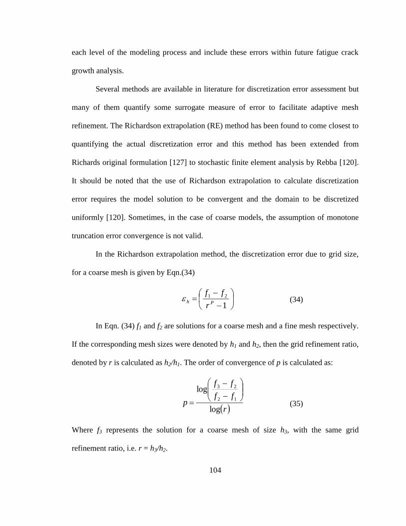
104
each level of the modeling process and include these errors within future fatigue crack
growth analysis.
Several methods are available in literature for discretization error assessment but
many of them quantify some surrogate measure of error to facilitate adaptive mesh
refinement. The Richardson extrapolation (RE) method has been found to come closest to
quantifying the actual discretization error and this method has been extended from
Richards original formulation [127] to stochastic finite element analysis by Rebba [120].
It should be noted that the use of Richardson extrapolation to calculate discretization
error requires the model solution to be convergent and the domain to be discretized
uniformly [120]. Sometimes, in the case of coarse models, the assumption of monotone
truncation error convergence is not valid.
In the Richardson extrapolation method, the discretization error due to grid size,
for a coarse mesh is given by Eqn.(34)
1
21
Phr
ff
(34)
In Eqn. (34) f1 and f2 are solutions for a coarse mesh and a fine mesh respectively.
If the corresponding mesh sizes were denoted by h1 and h2, then the grid refinement ratio,
denoted by r is calculated as h2/h1. The order of convergence of p is calculated as:
r
ff
ff
plog
log12
23
(35)
Where f3 represents the solution for a coarse mesh of size h3, with the same grid
refinement ratio, i.e. r = h3/h2.

105
The estimated discretization error will not be accurate if even the finest mesh used
in an analysis is not fine enough [121]. For this reason, initial convergence studies should
be performed to ensure that solution convergence is obtained from the model. The
Richardson extrapolation technique also requires that asymptotic convergence of the
finite element solution is observed when the mesh size is reduced, i.e. y1,y2,y3 in Eqn.
(35) should either progressively decrease or increase [128].
When using a global-local hierarchical finite element approach, it is necessary to
perform the Richardson Extrapolation technique on both the full model and sub model in
order to accurately represent the overall discretization error introduced within the
modeling process. As a result, finite element solutions were needed for 3 different mesh
densities within the full model while the sub model refinement was held constant, and
then solutions were needed for 3 different mesh densities within the sub model while the
full model refinement was held constant. By analyzing the solutions obtained from the
different mesh densities, modeling error could be estimated for each crack configuration
and loading condition.
The solutions f1, f2, f3 are dependent on the inputs (loading, current crack size,
aspect ratio and angle of orientation) to the finite element analysis and hence the error
estimates are also functions of these input variables. For each set of inputs, a
corresponding error is calculated and this error is added to the (coarse mesh) solution
from finite element analysis to calculate the true solution.
A series of finite element analyses were performed for various model input
combinations. For each model input combination, the model error resulting from the
meshing of the finite element model was evaluated using the Richardson extrapolation

106
technique. This analysis required three levels of discretization within the full model in
order to determine the rate of convergence and ultimately quantify the discretization error
associated with the coarsest mesh density. After performing the error analysis, it was
found that absolute value of error caused by the coarse mesh in the full model ranged
from 0.58% up to 3.53% depending on the crack configuration (length and aspect ratio)
and loading condition considered. A histogram of the model error is shown in Figure 38.
As indicated within the figure, it was determined that the distribution of the model error
fit the lognormal distribution function well, with a mean value of 2.144 and a variance of
0.154.
0.5 1 1.5 2 2.5 3 3.50
0.5
1
1.5
Percent Error
Percent Error using Richardson Extrapolation
Density
% Error (discretization)
Lognormal Distribution
Figure 38: Histogram of Percent Errors found during full-model refinement analysis
with results compared to lognormal distribution
Similar analysis can be performed to evaluate the discretization error caused by
the mesh choice within the sub model. In order to determine its effect on the overall
stress intensity factor solution, the full model mesh size is held constant while the mesh
density within the sub model is varied. For the sub model analysis, it is important to

107
accurately model the crack front with singular elements of adequate shape and size in
order to capture the stress state within the region, as more fully discussed in Section 3.3.
As a result, some limitations on the mesh density are necessary to ensure basic solution
convergence and non-irregular element shapes. After performing the Richardson
extrapolation analysis on the results obtained from the sub model refinement analysis, it
is found that the error caused by using even the coarsest mesh is relatively insignificant,
less than 1% for all cases. This is not a significant source of error for the purposes of
component life prediction and the discretization errors within the submodel are not
included in the overall probabilistic crack growth analysis.
It is not surprising that the discretization error evaluated for the submodel is
determined to be insignificant. This result can be explained by comparing the relative size
and mesh densities of the sub model when compared to the full model. The overall size
of the sub model is very small compared to that of the full model. As a result, the
relatively large elements in the full model are replaced by thousands of smaller elements
within the sub model. In order to maintain minimum element shape tolerances and
provide suitable mesh configurations for stress intensity factor calculations, even the
coarsest mesh density in the sub model analysis maintained a relative high mesh density
and provided accurate solutions.
The Richardson extrapolation technique has been shown to be a suitable way to
evaluate the inherent modeling errors that result from using a coarse mesh within a finite
element model, and has been applied to a hierarchical rotorcraft mast demonstration
problem. The method requires evaluating the model for three distinct mesh densities to
determine solution convergence rates. It should be noted that the discretization error

108
obtained using this method is a discrete error (as opposed to random error) that arises due
to the specific geometric configuration of the problem under consideration. As a result,
the modeling errors determined through this analysis should be directly added to the
corresponding stress intensity factors to provide adjusted solutions that more closely
match the true solution (void of any discretization errors). These “adjusted” model
solutions can be used to train the surrogate model as initially described in Section 4.5 and
analyzed within the next section. The histogram and distribution functions shown in
Figure 38 are included only to provide an overall summary of the individual results
obtained in this study and are not meant to (nor should they be) used for sampling
purposes in subsequent model evaluations.
4.3 Surrogate Model Error
The use of an efficient surrogate model allows for efficient cycle by cycle fatigue
crack growth evaluation for components subjected to variable amplitude multiaxial
loading by eliminating the computational burden that otherwise exists for calculation of
the stress intensity factor at the crack front. However, the surrogate model is itself an
approximation method to an already uncertain model, thus its use introduces another
uncertainty within the modeling framework that needs to be addressed.
The successful use of any surrogate modeling technique depends on the ability of
the surrogate to accurately match the underlying function shape, and a successful method
for identifying suitable data to most effectively train the surrogate. As discussed in
Section 3.5, the Gaussian process model is capable of accurately modeling the non-linear

109
relationship that exists between the input variables and output variables within the fatigue
crack growth modeling application. Therefore, the primary question is, if only limited
training points can be generated, which set of training points should be used to most
effectively train the surrogate model? The answer to the question depends on what
criteria (maximum error, average error, maximum variance, etc) is used to evaluate the
effectiveness of training, and several methods have been developed which approach this
problem from different perspectives. Three main methods offered within the literature
for training point selection are the traditional design of experiments [129], model error
minimization [130], and model variance minimization [106]. Within this research,
traditional DOE methods are first used to select a small set of initial training points,
followed by an iterative model variance minimization method using the Greedy point
algorithm. Details of the model error assessment resulting from the Gaussian Process
surrogate model is discussed below.
As detailed in Section 3.5, one of the advantages of using the Gaussian Process
surrogate modeling technique is that the method has the ability to provide a direct
representation of the uncertainty associated with its interpolative approximation. The
uncertainty in the model prediction is given by the model variance. The Greedy Point
algorithm can utilize the model variances across the entire design space to determine the
precise location which proves to have the largest model uncertainty (variance). The next
training point is set to be the combination of input variable values corresponding to that
particular location within the design space, the full FEA is evaluated to provide the
“correct” solution and is used to update the surrogate model. By repeating the Greedy
Point algorithm iteratively, training points can be identified that minimize the variance of

110
the surrogate model. This training point selection method eliminates the subjectivity
associated with typical design of experiments methods which use a pre-determined fixed
set of training points, and ensures that the surrogate model is iteratively improved by
adding new information that most efficiently reduces the maximum uncertainty in model
predictions.
50 100 150 200 250 300 350 400 450 5000
0.005
0.01
0.015
0.02
0.025
0.03
0.035
Number of Training Points
Maxim
um
Model V
ariance
Figure 39: Maximum GP model variance vs. # of Training points used
Table 5: Number of Training Points used in surrogate vs. Maximum Model Variance
# of Training Points Max. Model Variance
16 54.787240
24 1.145149
32 0.065271
40 0.040791
48 0.040660
56 0.009858
64 0.005758
72 0.002637
100 0.002064
200 0.000975
300 0.001683
400 0.000511
500 0.000542

111
Since the surrogate model is built using an iterative process, it is easy to track the
maximum model variance for different numbers of training points used. The maximum
model variance (model prediction uncertainty) is observed to decrease as additional
training points are used to train the surrogate. This trend can be clearly seen within
Figure 39 and Table 5 as the maximum model variance within the surrogate is shown as a
function of number of training points used. Since the model variance at any untested
location x* is based on its relative proximity to available training points as well as the
correlation structure between them, the overall variance is expected to decrease with
increasing training points within the design space.
The Greedy Point method which uses a model variance minimization technique
for training point selection has been compared to a recently proposed method which uses
a hierarchical decomposition of the approximation error for training point selection
method [130]. Comparisons of model predictions at different levels of training for the
fatigue analysis application described herein show the model variance and model error
minimization techniques to have very similar performance in terms of overall solution
accuracy.
For demonstration purposes, the Gaussian process model shown in Figure 39 was
trained for an overly large number of training points, as reflected by the small values of
model variance near the bottom of Table 5, resulting in a very small value of surrogate
model uncertainty. However, in practical applications where only limited finite element
runs may be possible, the associated surrogate model prediction uncertainty at different
locations within the design space may be more significant. The Gaussian process model
provides an easy and convenient method for quantifying the uncertainty in model
112
predictions when limited training points are available. Under these circumstances, model
predictions made using the surrogate model can be treated as Gaussian random variables
with closed form solutions for their mean values given by Eqn. (25) and variances given
by Eqn. (26). In doing so, the associated model uncertainty can be easily included within
the fatigue crack growth modeling framework.
4.4 Methodology to Incorporate Uncertainty in Final Prediction
The physical modeling process itself introduces many additional sources of
uncertainty that need to be accounted for in addition to the natural variability that is
inherent in physical processes. This chapter identified several uncertainties associated
with different types of numerical models that are typically used in fatigue crack growth
analysis. It is important that each of these uncertainties is quantified and included within
the stochastic fatigue crack growth modeling framework for component life prediction.
A systematic and rigorous probabilistic component life assessment can be performed by
combining the various sources of uncertainty detailed in Chapter 2, the modeling errors
discussed within this chapter, and the overall fatigue crack growth framework developed
in Chapter 3. Each input variable and modeling technique introduces additional
uncertainty that must be carefully combined within the analysis to provide a meaningful
and useful component life prediction under uncertainty.
The overall objective of a probabilistic damage tolerance analysis is to determine
the probability of component failure over the lifetime of the component. A sampling
methodology is used within this research to include many different sources of uncertainty

113
including physical variability, data uncertainty, and modeling errors. The approach
enables the evaluation of the distribution of the amount of time, t, for an initial flaw to
grow to a critical size, or conversely, the distribution of crack sizes at any time t . This
type of information can be used by fleet managers and maintenance personnel for
inspection planning and decision making. The various steps in this procedure are outlined
here.
I. Initial uncertainty quantification is performed to determine statistical distributions
of model parameters and input values including: material properties, crack growth
rate model parameters, and loading.
II. Component stress analysis is completed to identify critical crack location and
orientation
III. EIFS distribution is constructed from distributions of material properties (obtained
in step I) to statistically characterize the initial flaw size
IV. Finite element analysis is performed to provide necessary training points for the
Gaussian process surrogate model. Discretization error is evaluated and FEA
results using the coarse model are adjusted accordingly.
V. Updated FEA results are used for construction of initial GP model, and the Greedy
point algorithm is implemented to identify additional training points until a
satisfactory level of performance is reached
VI. The fully trained GP model is used exclusively for calculating the stress intensity
factor as a function of crack size, loading, aspect ratio and angle of orientation.
VII. A realization of a variable amplitude loading history is reconstructed using either
the rainflow or Markov reconstruction techniques.
114
VIII. A single realization of EIFS is sampled from its statistical distribution as calculated
based on material properties.
IX. For the current load cycle (obtained from history generated in Step VII), the stress
intensity factor is sampled from the GP model (where the mean and variance are
accounted for in model prediction) and the corresponding stress intensity factor is
used within a crack growth rate model to determine crack extension magnitude.
X. Cycle-by-cycle crack growth is evaluated at both the semi-major and semi-minor
locations along the crack front, thus allowing for semi-elliptical to semi-elliptical
crack shape development. Crack growth rate modeling is randomized by using
either the percentile or partial correlation approach detailed in Section 2.3. The
crack front is grown in plane and Steps IX and X are repeated until a critical crack
length is obtained.
XI. Steps VII X are repeated within a Monte Carlo scheme
The straightforward sampling procedure in combination with an efficient cycle-
by-cycle fatigue crack growth evaluation enables a multiple realization of fatigue crack
growth analyses to be performed quickly and without the need for much user
intervention. The analysis method enables the determination of statistical characterization
of fatigue crack sizes over time. Despite the addition of probabilistic representation of
model inputs, the computational efficiency afforded by the modeling framework enables
many simulations within the Monte Carlo framework to be performed without significant
computational expense.

115
A numerical example is included to show typical results that are obtained through
the use of this method. For this example, the material considered is aluminum alloy 7075-
T6. The material properties of the aluminum alloy are included within Table 6.
Table 6: Material Properties of 7075-T6 Aluminum alloy
7075-T6 Aluminum Alloy
SI Units US Units
Modulus of Elasticity 71.7 GPa 10400 Ksi
Poisson Ratio 0.33 0.33
Yield Stress 503 MPa 73 Ksi
Ultimate Stress 572 MPa 83 Ksi
A Monte Carlo based method is used to perform the analysis method outlined
above. Typical results obtained within each step have been previously presented within
the original sections in which they were presented, and therefore, will not be repeated
here. As mentioned previously, the Monte Carlo implementation generates a random
realization of each stochastic variable and performs a cyclic fatigue crack growth analysis
from an initial size to a final size using either the percentile or partial correlation fatigue
crack growth rate representation. The crack growth results obtained from all realizations
can then be used to determine the statistics of the fatigue life predictions under
uncertainty.
Figure 40 and Figure 41 show numerical crack growth modeling results obtained
from the stochastic fatigue crack growth analysis procedure using both the percentile and
partial correlation crack growth rate modeling approaches. Similar simulation results are
obtained using either stochastic crack growth rate representations indicating that the
choice in stochastic crack growth rate representation (percentile and partial correlation)

116
does not have a significant effect on the overall fatigue life prediction. Each method
appears to equally represent the scatter in the fatigue crack growth rate data and results in
the same overall model prediction when all the other sources of uncertainty are
considered. A typical crack profile which results from the planar crack growth analysis is
shown in Figure 42 after many crack growth increments are completed.
0 5 10 15
x 104
0.5
1
1.5
2
2.5x 10
-3
Number of Load Cycles
Cra
ck S
ize (
m)
Figure 40: Plot showing simulated fatigue crack growth curves considering natural
variability, information uncertainty, and modeling error

117
0 0.2 0.4 0.6 0.8 1 1.2 1.4 1.6 1.8 2
x 105
0.5
1
1.5
2
2.5
x 10-3
Number of Load Cycles
Cra
ck S
ize
(m
)
Mean
90% Bound
(a.)
0 0.5 1 1.5 2
x 105
0.5
1
1.5
2
2.5
x 10-3
Number of Load Cycles
Cra
ck S
ize
(m
)
Mean
90% Bound
(b.)
Figure 41: Plot showing mean and 90% confidence bounds on component life prediction
obtained using the a.) percentile b.) partial correlation crack growth rate representations
The probabilistic crack growth method not only can provide a mean prediction for
component fatigue life, but can also estimate the variance to be expected in life prediction
considering uncertainty, as seen in Figure 41 a) and b.). One of the key benefits of using
the probabilistic based modeling approach is the ability to extract from the simulation
results a crack size probability distribution at any given time, t, or, conversely the
probability distribution of the time necessary for a crack to reach a critical size. These

118
results can be easily expressed through statistical distributions functions. Figure 43 a.)
and b.) show simulation results with the lognormal probability density function and
cumulative density function, respectively, for the number of load cycles necessary for an
initial crack to grow to a critical size extracted from the results obtained using the
percentile crack growth rate representation. Similar statistical distributions can be
evaluated to represent the crack size population after any given number of load cycles.
-0.06 -0.04 -0.02 0 0.02 0.04 0.060
0.01
0.02
0.03
0.04
0.05
0.06
0.07
0.08
0.09
0.1
Crack Length (in.)
Cra
ck D
epth
(in
)
Crack Shape Developement
Mixed Mode Proportional Loading
Figure 42: Typical fatigue crack profile showing crack growth due to fatigue loading

119
1 1.5 2 2.5 3 3.5 4 4.5 5
x 105
0
1
2
3
4
5
6
7
x 10-6
Data
Density
PDF of Cycles to Critical Crack Size
Simulation Results
Lognormal Distribution
(a.)
1 1.5 2 2.5 3 3.5 4 4.5 5
x 105
0
0.1
0.2
0.3
0.4
0.5
0.6
0.7
0.8
0.9
1
Data
CDF of Cycles to Critical Crack Size
Cum
ula
tive p
robabili
ty
Simulation Results
Lognormal Distribution
(b.)
Figure 43: a.) PDF and b.) CDF of Lognormal distribution function of number of cycles
to reach a critical crack size shown with simulation results
The use of various models for the analysis of complex system performance
incorporates many approximations and assumptions which result in errors in model
predictions. This chapter has presented methods to evaluate different types of modeling
errors including finite element discretization error and surrogate modeling error and has
120
demonstrated how uncertainties at all levels of the crack growth modeling approach can
be incorporated within an overall probabilistic fatigue life assessment.
Both deterministic and random errors have been addressed within this work and
can easily be included within the overall probabilistic crack growth modeling framework.
Finite element discretization errors represent deterministic errors that result from the
specific mesh densities used within finite element models. Error resulting from using a
coarse mesh density is determined using a Richardson extrapolation technique and is a
deterministic error should be evaluated and directly applied to the model prediction.
Deterministic errors should not be treated using sampling techniques as their effects are
directly related to specific configurations. The stress intensity factors evaluated using the
Gaussian Process (GP) surrogate model represent uncertain model predictions, which
produce random model errors. These types of errors can be included by sampling
techniques.
Multiple sources of uncertainty including natural variability, data uncertainty, and
modeling errors can be incorporated into the methods developed in previous chapters.
The methods for implementation of the developed methodology to a realistic rotorcraft
component have been provided within this chapter and executed on the rotorcraft mast
demonstration problem. Overall, the fatigue crack growth framework developed in
Chapter 3 is capable of performing cycle-by-cycle fatigue crack growth analysis while
considering several different sources of uncertainty in model input values and parameters
described in Chapter 2 as well as model errors which have been classified in this chapter.

121
CHAPTER V
NON-PLANAR FATIGUE CRACK GROWTH MODELING
5.1 Introduction
Damage tolerance based design has increased the necessity for better
understanding of fatigue crack growth mechanisms in mechanical components.
Traditional applications of fracture mechanics, as well as most experimental testing, have
focused on cracks growing under pure mode I conditions. Characterization of fatigue
crack growth under Mode I loading conditions using the stress intensity factor range is
based on the assumption that the path of the crack is linear and that its plane of growth is
normal to the loading axis [131]. Therefore, the crack growth direction remained in plane
with the original crack orientation, resulting in planar (non-kinked) cracks even after the
occurrence of several crack growth increments. The fatigue crack growth modeling
framework developed in Chapter 3 adopted this approach for probabilistic fatigue life
prediction under uncertainty.
It is, however, well known that on a microscopic level, cracks seldom propagate
in a linear fashion (even under Mode I loading), and on a macroscopic level, cracks in
structures are often subjected to mixed-mode conditions, resulting in crack kinking and
other non-planar propagation paths. As a result, there is a growing interest in
investigating the mechanics and crack growth modeling capabilities associated with the
nonlinearities in the crack path. When considering non planar crack growth modeling, it
is important to be able to predict and model both the crack extension magnitude and the

122
crack path direction. Nonlinearities in the crack path have been generally ignored in
fatigue life prediction because of the difficulties in incorporating crack meandering
effects in estimates of the stress intensity factor range [131], crack extension criteria, and
crack model meshing capabilities. In order to try to capture the nonlinear crack extension
behavior that has been seen in both experimental results and realistic applications,
numerous crack growth direction and extension criteria have been proposed within the
literature by different authors over the past few decades. This chapter will investigate the
fatigue crack growth modeling capabilities for non-planar fatigue cracks. Additionally, it
will provide a suitable method for fatigue crack growth simulation with the goal of
investigating the uncertainty in crack path and component life predictions resulting from
different criteria for crack extension magnitude and direction.
There are two dominant modes of fatigue crack propagation: tensile and shear
dominated crack growth [132]. Tensile dominated crack growth is also sometimes
referred to as maximum principal stress dominated, and is the class most often observed
in metal fatigue. Under the tensile dominated case, a Mode I crack usually (but not
always) tends to propagate in a direction that is perpendicular to the maximum principal
tensile stress within the uncracked specimen [133]. The second dominant mode is shear
dominated crack propagation (Mode II type), which usually takes place on planes of
maximum shear stress and is an important exception to the tendency to Mode I fatigue
crack propagation [134]. In metal fatigue, the shear dominated mode of crack propagation
is often observed when the crack tip plastic zone becomes large, and is generally
applicable to micro cracks that are characterized as stage I cracks in Forsyth's notation
[143] (as shown in Figure 45). Additionally, a third mode of fatigue crack propagation is

123
sometimes observed and is called slant crack propagation. This type is another exception
to Mode I, and is often observed in thin sheets and is characterized by a transition zone
between Mode I and Mode III fatigue growth. A schematic of generalized crack growth
under mixed mode loading is shown in Figure 44.
Figure 44: Schematic showing development of fracture surface for a.) in plane crack
opening subjected to mode I; b.) crack kinking under mode II; c.) crack front twisting
under mode III; d.) deflected crack for superimposed modes I, II, and III
In the last four decades there have been substantial advances in the understanding
of macroscopic aspects of fatigue crack paths and their prediction [134]. However, at the
present state of the art, the factors controlling the path taken by a propagating fatigue
crack are not completely understood, and, in general, crack paths are difficult to predict
[134]. Under mixed mode loading, the fatigue crack growth rate is typically expressed
[134,163] with the same functional relation as that of the uniaxial case where the stress
intensity factors in multiple modes are replaced by a single equivalent stress intensity
factor range, ΔKeqv.
eqvKf
dN
da
(36)

124
One approach that is commonly seen within the literature is to ignore any
nonlinearity in the crack path direction due to the difficulties in incorporating crack
meandering effects in estimates of the stress intensity factor range. Fatigue crack path
prediction for a planar crack is essentially two dimensional, regardless of whether a
single point, two point, or multiple point extension criterion is used. Ultimately, it
reduces to making the assumption that crack propagation direction is perpendicular to the
current crack front, and calculating crack growth increment (s) using a standard crack
growth law, such as one listed in Table 1. Many of the existing three-dimensional
fracture simulation codes actually fall under this category since only planar crack
extension is considered.
Theoretical justifications for a planar crack growth assumption are that local
variations in the path of a long fatigue crack are normally overcome during subsequent
propagation over a short distance under certain loading conditions [131], and that
projection of the initial mixed mode crack onto an appropriate plane can provide an
accurate method for estimating SIFs for a kinked crack [135]. Additionally, it has been
pointed out by numerous authors that on a macroscopic scale, and under essentially
elastic conditions, most fatigue cracks in isotropic metallic materials tend to propagate in
Mode I [134], that is, approximately perpendicular to the maximum principal tensile
stress. These authors include Borberg [136], Cotterell [137], Knauss [138], Minoshima
[139], Parton[140], Pook [133,141], and Vinas-Pich [142]. Under this observation,
cracks that are classified to stage II in Forsyth's notation [143] often show crack growth
behavior that is confined to a particular plane [143].
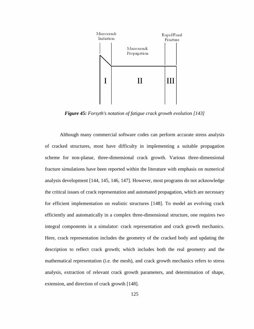
125
Figure 45: Forsyth's notation of fatigue crack growth evolution [143]
Although many commercial software codes can perform accurate stress analysis
of cracked structures, most have difficulty in implementing a suitable propagation
scheme for non-planar, three-dimensional crack growth. Various three-dimensional
fracture simulations have been reported within the literature with emphasis on numerical
analysis development [144, 145, 146, 147]. However, most programs do not acknowledge
the critical issues of crack representation and automated propagation, which are necessary
for efficient implementation on realistic structures [148]. To model an evolving crack
efficiently and automatically in a complex three-dimensional structure, one requires two
integral components in a simulator: crack representation and crack growth mechanics.
Here, crack representation includes the geometry of the cracked body and updating the
description to reflect crack growth; which includes both the real geometry and the
mathematical representation (i.e. the mesh), and crack growth mechanics refers to stress
analysis, extraction of relevant crack growth parameters, and determination of shape,
extension, and direction of crack growth [148].

126
For the case in which the initial fatigue crack is allowed to grow in a non-planar
fashion, both crack extension and crack direction model predictions are necessary and
lead to an increase in the complexity of the crack shape development and computational
modeling considerations. The following section discusses many of the existing non-
planar crack growth criteria which have been reported within the literature with particular
emphasis on the various theoretical and empirical forms available for the crack kink
angle and equivalent stress intensity factor under mixed mode I, II, and III conditions.
Section 5.3 provides details of the specific methods which are used for component stress
analysis and non-planar crack modeling within this research. The remaining sections of
this chapter focus on the challenges associated with surrogate modeling development for
non-planar crack growth analysis and a proposed equivalent planar method which links
the insight obtained using a more sophisticated non-planar crack growth analysis to the
planar crack growth analysis presented in earlier chapters of this dissertation.
5.2 Existing Non-Planar Crack Growth Criterion
For the case of mixed mode I + II loading and non-planar crack growth modeling,
the most commonly used criterion for tensile crack propagation is the maximum
tangential stress (MTS) criterion as proposed by Erdogan and Sih (1963) [149]. The
tangential stress, σθ, near the tip of a crack subjected to mixed I+II mode is expressed by
sin
2
3
2cos
2cos
2
1 2
III KKr
(37)
where the crack deflection angle, θσ, can be obtained from solving the equations

127
0|
0
and 0|
02
2
(38)
which yields the angle, θσ, at the maximum σθ that is obtained from the expression
0)1)cos(3()sin( III KK
(39)
The equivalent SIF for mode I, ΔKIeqv, for mixed mode cracks is then given by the
expression
)
2sin()
2(cos3)
2(cos 23
,
IIIeqvI KKK
(40)
where ΔKI, ΔKII are the mode I and mode II stress intensity factors for the initial crack,
and θ is the crack propagation angle.
Richard [150] later approximated the ΔKIeqv expression given by Erdogan and Sih for
Mode I+II as
2222
, 62
1
2)(4
2
1
2III
I
III
I
eqvI KKK
KKK
K
(41)
and also approximated the crack deflection angle by
2
4.835.155
III
IIo
III
IIo
KK
K
KK
K (42)
which has been proven to be a good approximation by a large number of experiments
[151]. Richard later extended previous approximation functions to be used for crack
growth prediction under the general mixed mode I+II+III loading case. The function in
Eqn. (42) has been extended to the three dimensional case as follows
2
IIIIII
II
IIIIII
II
KKK
KB
KKK
KA
(43)

128
where θo<0o for KII>0 and θo>0
o for KII<0 and KI≥0. The equivalent stress intensity
factor is then suggested to take the form of
2
2
2
1
2 )(4)(42
1
2IIIIII
Ieqv KKK
KK
(44)
With α1=KIC/KIIC=1.155 and α2=KIC/KIIIC=1.0, excellent agreement has been observed
with that obtained from the σ1' criterion (given in Eqn. (61) ).
Pook [141] made another approximation to the original MTS criterion with the
expression
5.1
34489.083.022
IIII
eqv
KKKK
(45)
And Yan [152] suggested another functional form for mixed mode I+II loading given by
sin3cos1)2
cos(2
1IIIeqv KKK
(46)
where θσ is the crack growth direction obtained from the maximum tangential stress
criterion determined through Eqn. (38).
Tanaka [153] proposed the parameter
4/144
8 IIIeqv KKK
(47)
which can be extended to the Mode I+II+III case as follows
4/14
44
)1(
88
III
IIIeqv
KKKK
(48)
or, based on the energy release rate criterion for mixed mode I+II,
2/122
IIIeqv KKK
(49)
and for the extended to the Mode I+II+III case as

129
2/1222
)1( IIIIIIeqv KKKK
(50)
The rate of mixed mode crack propagation using any of these criteria is higher than that
predicted from ΔKI only, and the inclusion of mode II and III stress intensity range is
necessary in the crack propagation law [156].
Another criterion that has been used for the tensile crack growth direction is the
Local Symmetry (LS) criterion proposed by Kitagawa [154]. The LS criterion assumes
that a crack propagates in the direction where the mode II stress intensity factor of a
kinked crack is zero, and the stress field is symmetrical with respect to the mode I crack.
Additionally, the maximum strain energy release rate criterion proposed by Palaniswamy
and Knauss [155] assumes that the crack grows in the direction where the strain energy
release rate is the maximum and that the maximum value is a material constant. The
crack growth directions predicted by the LS criterion and the maximum strain energy
release criterion are generally very close to the direction predicted by the MTS criterion
[156].
For shear mode fatigue crack growth, the maximum shear stress (MSS) criterion
proposed by Otsuka [157] has been used. The shear stress, trθ, near the crack tip is given
by
)1cos3(
2
1sin
2
1
2cos
2
1
IIIr KK
rt
(51)
where the angle, θr, for the maximum shear stress, trθ, is
0)1cos3(2
tan2)1cos3(
IIt
tIt KK
(52)
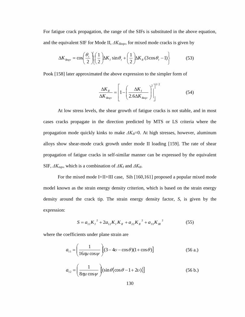
130
For fatigue crack propagation, the range of the SIFs is substituted in the above equation,
and the equivalent SIF for Mode II, ΔKIIeqv, for mixed mode cracks is given by
)1cos3(
2
1sin
2
1
2cos tIItI
tIIeqv KKK
(53)
Pook [158] later approximated the above expression to the simpler form of
2/12
6.21
IIeqv
I
IIeqv
II
K
K
K
K
(54)
At low stress levels, the shear growth of fatigue cracks is not stable, and in most
cases cracks propagate in the direction predicted by MTS or LS criteria where the
propagation mode quickly kinks to make ΔKII=0. At high stresses, however, aluminum
alloys show shear-mode crack growth under mode II loading [159]. The rate of shear
propagation of fatigue cracks in self-similar manner can be expressed by the equivalent
SIF, ΔKeqv, which is a combination of ΔKI and ΔKII.
For the mixed mode I+II+III case, Sih [160,161] proposed a popular mixed mode
model known as the strain energy density criterion, which is based on the strain energy
density around the crack tip. The strain energy density factor, S, is given by the
expression:
2
33
2
2212
2
11 2 IIIIIIIII KaKaKKaKaS
(55)
where the coefficients under plane strain are
)cos1)(cos43(cos16
111
a
(56 a.)
)21cos(sincos8
112
a
(56 b.)

131
)1cos3)(cos1()cos1)(1(48
122
Ea
(56 c.)
cos4
133a
(56 d.)
where μ is the shear modulus of elasticity and is Poisson's ratio. The crack angles, θ
and ψ are derived by minimizing S
0
S and 0
o
S
(57)
Crack extension occurs when the strain energy density factor reaches a critical value in a
direction defined by θo, which corresponds to the direction of minimum strain energy
density. For cyclic loading, a cyclic strain energy density factor is defined by
III
mean
IIIoII
mean
IIoII
mean
II
mean
IIoI
mean
Io KKaKKaKKKKaKKaS )()())((2)(2 33221211
(58)
which includes both the stress range and the mean stress, and can be used after
determining the direction of crack growth from Eqn. (57). The crack growth rate is
directly related to ΔS through the expression
2/)( m
s SCdN
da
(59)
where
2/
)1)(21(
2m
s
ECC
(60)

132
Schollmann [162] proposed the σ1' crack growth criterion that also can be applied to the
three dimensional case. The criterion is based on the assumption that crack growth
develops perpendicularly to the direction of σ1', which is a special maximum principal
stress. σ1' can be defined by the near-field stresses σθ, σz, and τθ,z as follows
22'
1 42
1
2zz
z
(61)
Due to the assumption that the crack growth direction is perpendicular to σ1' , the crack
deflection angle, θo, can be calculated by
0'
1
o
and 0
2
'
1
2
o
(62)
After substituting the near-field stress solutions and differentiating partially with respect
to θ, the following formulation can be found
2tan126
2tan6 2
III KK
2
222
2tan1
2tan32
2tan126
2tan6
2tan124
IIIIIIIII KKKxKK
2/12
22
2
2tan164
2tan124
IIIIII KKKx
(63)
The equivalent stress intensity factor can then be calculated as
2
2
22 42
sin2
3
2cos
2sin
2
3
2cos
2cos
2
1III
oII
oI
oII
oI
oeqv KKKKKK
(64)

133
As evident from the lengthy discussion above, numerous criteria have been developed to
approximate the crack kinking phenomenon that has been observed under mixed mode
loading conditions for both the crack kinking direction and equivalent stress intensity
factor solutions. For mixed I+II+III mode loading conditions a good literature review can
be found in Richard [163], Tanaka [156], and Marquis and Socie [164]. Additionally, the
work by Liu [165] provides a thorough review of both S-N based multiaxial fatigue
models as well as mixed mode fatigue crack growth models.
While various theoretical models to predict non-planar crack kinking behavior
have been proposed, none has been widely accepted as a universal theory. Each of the
above criterions is different from the others, but it is not clear exactly how much
difference will be observed in the fatigue life prediction resulting from each criterion.
Some criteria may predict similar crack trajectories and only slight differences will exist,
while others may result in significantly different crack paths and fatigue life predictions.
In addition to the mathematical representation of the fatigue crack path prediction
provided by the equations above, it is also necessary to be able to incorporate the crack
direction modeling approach within the current finite element model. There needs to
exist a method to update crack shapes and sizes within the finite element model for
accurate determination of the local stresses at the crack tip for various cracked
configurations. For the three-dimensional fatigue crack problem, where surface cracks
can grow in a non-planar fashion with different kink angles along the entire crack front,
creating robust crack extension and local remeshing algorithms for all of the criteria
mentioned above is not a trivial task. It is impractical to try to evaluate all of the
candidate non planar fatigue crack growth models as a result of the high computational

134
expense and implementation time necessary to do so. Therefore, for the purposes of this
research, only a few of the most common models are evaluated.
5.3 Component Stress Analysis and Non-Planar Crack Modeling
The software Fracture Analysis Code in 3-Dimensions/Next Generation
(FRANC3D/NG) is used for its crack insertion and local remeshing algorithms which
help to simplify the modeling complexities that exist in modeling the non-planar fatigue
crack growth problem using finite element software. FRANC3D/NG is a newer version
of the original FRANC3D crack growth simulation software package developed by the
Cornell Fracture Group and the Fracture Analysis Consultants [166]. In addition to other
improved features, FRANC3D/NG uses finite element software instead of the boundary
element method for component stress analysis and incorporates both stress analysis and
crack propagation capabilities within its construct. FRANC3D/NG has the capability to
adaptively insert and extend cracks and/or voids in pre-existing finite element meshes,
and has been developed to work in conjunction with commercial finite element software
packages such as ANSYS, ABAQUS, and NASTRAN.
For the non-planar crack growth framework within this study, stress analysis is
performed using the ANSYS version 11.0 commercial software package, same as in
Chapter 3 for planar cracks. Initial crack insertion within the finite element model is
performed within the FRANC3D/NG software and local remeshing at the crack location
is performed using crack tunnel and singular elements at the crack front as presented in
Section 3.3. Once a crack is inserted into a finite element model, the commercial finite
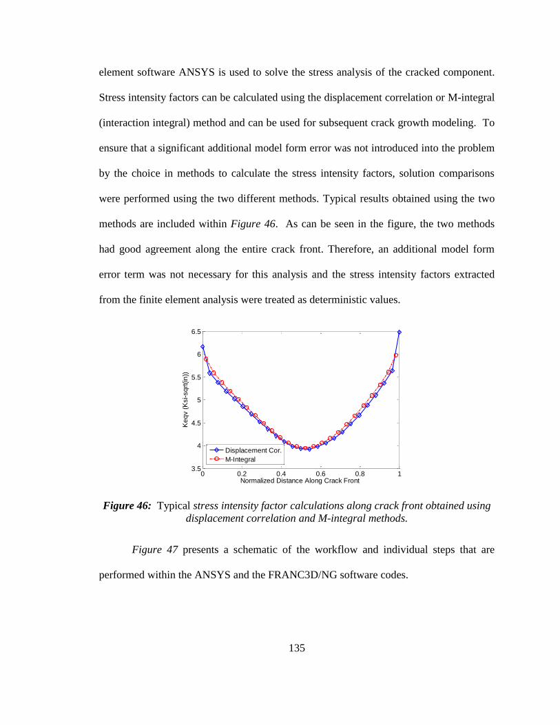
135
element software ANSYS is used to solve the stress analysis of the cracked component.
Stress intensity factors can be calculated using the displacement correlation or M-integral
(interaction integral) method and can be used for subsequent crack growth modeling. To
ensure that a significant additional model form error was not introduced into the problem
by the choice in methods to calculate the stress intensity factors, solution comparisons
were performed using the two different methods. Typical results obtained using the two
methods are included within Figure 46. As can be seen in the figure, the two methods
had good agreement along the entire crack front. Therefore, an additional model form
error term was not necessary for this analysis and the stress intensity factors extracted
from the finite element analysis were treated as deterministic values.
0 0.2 0.4 0.6 0.8 13.5
4
4.5
5
5.5
6
6.5
Normalized Distance Along Crack Front
Ke
qv (
Ksi-sq
rt(in
))
Displacement Cor.
M-Integral
Figure 46: Typical stress intensity factor calculations along crack front obtained using
displacement correlation and M-integral methods.
Figure 47 presents a schematic of the workflow and individual steps that are
performed within the ANSYS and the FRANC3D/NG software codes.

136
Figure 47: Work flow chart of FRANC3D/NG and finite element software for non-planar
fatigue crack modeling
At the present time, no universally accepted non-planar three-dimensional crack
extension criteria currently exists, however, many two-dimensional models have been
presented in the literature. The current state of the art for three-dimensional crack
extension modeling is to evaluate the crack propagation direction at several discrete
points along the crack front using two-dimensional plane strain equations. Plane strain
equations are applied in the plane normal to the crack front tangent to determine the
direction of propagation using one of several available crack propagation criteria. This
technique effectively reduces the three-dimensional crack growth problem to a series of
two-dimensional problems, evaluated at discrete points along the crack front.
The application of this method results in the relative extension of each node along
the crack front based on local stress conditions at that specific location. The result of this
137
approach is a theoretical new crack front shape and location, based on a finite number of
nodes. In order to maintain suitable finite element meshes at the crack front location, a
best fit polynomial function is used to represent the updated crack front location. In doing
so, a necessary approximation is made to the predicted crack front location leading to a
smoother crack front representation than was initial predicted by the theoretical models.
However, the suitability of this approximation can be monitored throughout the crack
growth simulation to ensure that a reasonable crack front representation is maintained.
Figure 48 a.) shows an example of a non-planar crack growth analysis where a
theoretical crack front location is indicated by the green nodal positions and the best fit
location is shown by the blue nodal locations and the “crack tunnel”. Additionally, this
relationship can also be shown through simple plots such as that one shown in Figure 48
b.), which depicts the theoretically predicted nodal extensions by the individual dots and
the best fit polynomial by the solid line (with good correspondence shown here for a 3rd
order polynomial).

138
(a.) (b.)
Figure 48: Non-planar crack growth analysis showing crack surface as well as predicted
and „best fit‟ crack extension locations
For the purpose of this work, two common crack direction modeling criteria will
be evaluated within the non-planar crack growth framework; the maximum tangential
stress (MTS) criterion, and the modified strain energy release rate criterion. These criteria
are chosen based on the fact that they have already been incorporated within the
FRANC3D/NG code, as well as for the familiarity of the fatigue research community
with their functional forms.
For the general mixed mode I+II+III condition, the maximum tangential stress
criterion identifies the crack kinking angle, θ, as given in Eqn. (65)
Kink
such that
MAX
(65)
and a transition to the maximum shear stress criterion can be incorporated by including
shear terms, which results in the expression

139
max
2
2
2
2
max |,| z
IIIC
ICr
IIC
IC
K
K
K
KMAX
(66)
where KIC , KIIC ,and KIIIC are the mode I, mode II, and mode III fracture toughness
values. The modified strain energy release rate criterion identifies the crack kinking
angle, θ, as given in Eqn. (67)
Kink
such that
max| and max
2
2
2| r
IIC
IC
K
K
(67)
For crack growth modeling, stress analysis is performed on the cracked
component, and the local stress conditions are used within either the maximum tangential
or the modified strain energy release rate models to determine crack extension directions
at discretized points along the crack front. Stress intensity factors are evaluated from the
local stress results and the relative advance at each point along the crack front can be
evaluated using a crack growth law.
Several options exist for modeling crack extension magnitude, including cycle-
by-cycle, incremental block-type, and median extension based approaches. For the cycle-
by-cycle crack growth, crack extensions are performed for each and every load cycle
using traditional fatigue crack growth laws, such as those presented in Table 1.
Although the cycle-by-cycle approach is considered to be the most accurate of the above
crack growth modeling approaches, it also presents significant computational challenges
during numerical evaluation. For the high cycle fatigue problem, much of the crack
growth occurs in the near threshold and the lower portion of the Paris/linear region of the

140
fatigue crack growth curve (shown schematically in Figure 3). Cycle-by-cycle crack
extension within these regions is of the order of 10-10
- 10-8
in/cycle, meaning hundreds of
thousands of individual stress analyses, crack extensions, and local remeshing functions
are needed to double the size of an initial crack of 0.01 inch.
In addition to the substantial computational expense that the cycle-by-cycle
approach demands, other limitations exist in the forms of mesh size and crack shape
representations. In theory, the minimum element size contained within the mesh must be
able to capture the crack profile. Therefore, to accurately represent cyclic crack extension
within the near threshold region, the mesh size must be of the order of the crack
extension, that is ~10-10
inches, resulting in an unacceptably large number of elements
contained within the finite element model. For non-planar crack propagation, not only is
the extension magnitude calculated for each analysis, but also the direction of crack
growth is necessary. For the cycle-by-cycle case, each individual crack growth step may
have different propagation directions, leading to a highly complex, small scale zigzag
type crack path. Again, this type of crack profile across the entire crack front presents
problems for accurately and efficiently remeshing the crack front. From a computational
time and numerical stability standpoint, a more reasonable crack propagation approach
must be adopted.
An alternative to the cycle-by-cycle approach is to adopt a block-type crack
growth extension method. This approach is similar to that of the cycle-by-cycle approach,
with the exception that crack extension and direction modeling is held constant over a
user-defined number of cycles. The block-type extension technique is based on the idea

141
of extending points along the crack front by a multiple of the crack growth increment
determined for a single load cycle. Mathematically, this can be represented as
iuser
i
userupdate aNdN
daNa **
(68)
where Δaupdate is the total crack growth applied to the current crack, Nuser is the user
defined block increment, and idN
da
is the crack growth magnitude for the current load
cycle. This method allows for cyclic based crack extension, without requiring crack
updating and remeshing for every load cycle, and is well suited to represent block-type
loading conditions where the load history is composed of many sub-blocks of constant
amplitude loading.
The median extension crack growth approach can also be used to overcome both
the efficiency and stability issues that are inherent in the cycle-by-cycle approach. The
median extension technique is based on the idea of extending points along the crack front
in some proportion to a user-defined extension length. The proportion of crack extension
at a given location is determined from the ratio of the stress intensity at that location
compared to the mean stress intensity factor found at any point along the entire crack
front. Mathematically, this relationship can be represented as given in Eqn. (69).
mean
inode
meanuserinodeK
Kfaa
_
__ *
(69)
where Δauser_mean is the user-defined allowable median crack length extension. Using this
formulation, the stress intensity factor at each crack front node is evaluated , ΔKnode_i, and
crack extension is evaluated by comparing the stress intensity factor at that location to the
mean stress intensity factor obtained along the entire crack front, ΔKmean. The parameter f
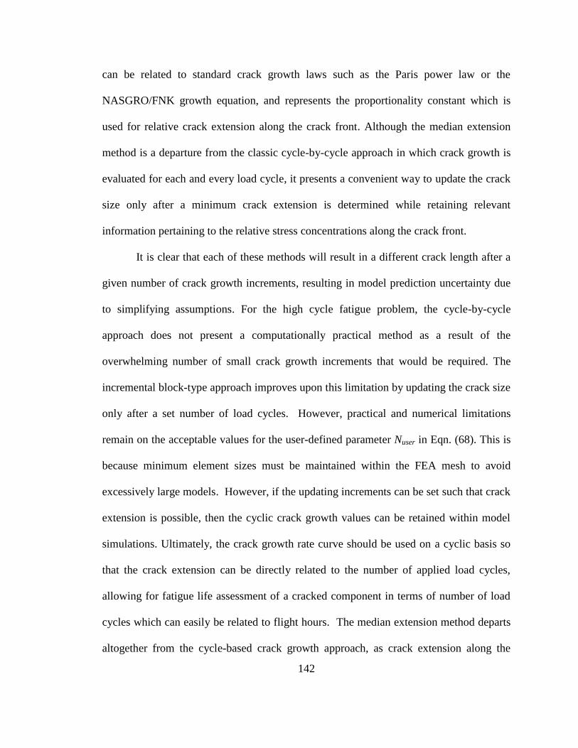
142
can be related to standard crack growth laws such as the Paris power law or the
NASGRO/FNK growth equation, and represents the proportionality constant which is
used for relative crack extension along the crack front. Although the median extension
method is a departure from the classic cycle-by-cycle approach in which crack growth is
evaluated for each and every load cycle, it presents a convenient way to update the crack
size only after a minimum crack extension is determined while retaining relevant
information pertaining to the relative stress concentrations along the crack front.
It is clear that each of these methods will result in a different crack length after a
given number of crack growth increments, resulting in model prediction uncertainty due
to simplifying assumptions. For the high cycle fatigue problem, the cycle-by-cycle
approach does not present a computationally practical method as a result of the
overwhelming number of small crack growth increments that would be required. The
incremental block-type approach improves upon this limitation by updating the crack size
only after a set number of load cycles. However, practical and numerical limitations
remain on the acceptable values for the user-defined parameter Nuser in Eqn. (68). This is
because minimum element sizes must be maintained within the FEA mesh to avoid
excessively large models. However, if the updating increments can be set such that crack
extension is possible, then the cyclic crack growth values can be retained within model
simulations. Ultimately, the crack growth rate curve should be used on a cyclic basis so
that the crack extension can be directly related to the number of applied load cycles,
allowing for fatigue life assessment of a cracked component in terms of number of load
cycles which can easily be related to flight hours. The median extension method departs
altogether from the cycle-based crack growth approach, as crack extension along the

143
crack front is dictated by user input as opposed to number of applied load cycles. This
approach arbitrarily imposes crack extensions in an attempt to ensure numerical stability
and to better manage the relative extensions of the crack front at each load step.
Depending on the characteristics of the applied load history as well as the overall
goal of the numerical simulation, either the incremental or the median extension method
might be more appropriate.
5.4 Surrogate Model Development
Response surface methodology can be used in place of expensive finite element
models for iterative fatigue analysis to reduce the computational effort needed to
calculate the stress intensity factor at the crack tip. This is particularly useful in
uncertainty analysis where multiple simulations of cycle-by-cycle crack growth analysis
have to be executed. In Chapter 3, a response surface approximation was developed to
approximately capture the relationship between the input variables (crack length, shape,
and load value) and the output variable (mixed mode stress intensity factor) within the
planar fatigue crack growth modeling framework. The finite element model was used to
"train" a Gaussian process surrogate model to an acceptable degree of accuracy by
evaluating the FEA at selected points within the design space identified by using the
greedy point algorithm. The use of a surrogate model drastically improves the
computational effort needed to perform crack growth analysis by eliminating the need for
repeated evaluation of the full finite element model for each load cycle and crack
configuration.

144
A surrogate modeling approach would provide extremely useful within the non-
planar fatigue crack growth modeling framework for similar reasons. However,
construction of a meaningful and useful surrogate model for the non-planar crack growth
case is a significant challenge for several reasons. The first major obstacle in constructing
a surrogate model is how to precisely define the three-dimensional complex crack shape.
The crack shape for a non-planar three-dimension crack depends on the surface crack
length, crack depth, and the individual kink angles along the crack front for each previous
crack growth evaluation. As opposed to the planar crack shape, which could be well
characterized by a few simple parameters, the non-planar crack shape is most fully suited
to characterization by a three-dimensional, undulating surface. Therefore, crack
characterization using basic parameters becomes a challenge. As a result, it is difficult to
define the input parameters for crack characterization to be used to train the surrogate
model.
A further challenge exists in the capability to generate complex crack
configurations. Within the current non-planar modeling framework, a simple crack is
introduced into the structural component and then is allowed to evolve into a non-planar
crack due to the applied loading and crack extension criteria. As a result, complex crack
shapes develop from simpler shapes over time, rather than being inputted directly. The
capability to generate and evaluate any possible crack configuration are necessary and an
accurate and efficient method to accomplish this is not currently available.
Another major complication in developing a surrogate model for general three-
dimensional non-planar crack growth analysis is related to the form of the predicted
model outputs. For this application, the nodal extension magnitude and directions are

145
needed to be predicted for each crack configuration. This means that the number of nodes
along the crack front is known a priori, the surrogate model can identify and
appropriately handle physical model boundaries, and that the surrogate modeling method
itself is capable of predicting multiple output values in vector form.
Currently, these limitations present a significant challenge for easy extension of
the surrogate modeling approach developed in Chapter 3 to the non-planar crack growth
framework investigated in this chapter. Further research is needed to expand the current
modeling approach in this application.
5.5 Equivalent Planar Method
An equivalent planar approximation is presented within this section as a method
which may be valuable for reducing the computational expense of performing non-planar
fatigue crack analysis within a probabilistic framework. The method creates a link
between the non-planar crack growth analysis methods presented within this chapter, and
the simpler planar crack growth analysis method described in Chapter 3. The method
aims to retain valuable information obtained through initial non-planar crack propagation
analyses for use within the planar analysis.
The basic idea behind the modeling approach is to try to use the results from the
non-planar fatigue crack growth analyses to identify crack characteristics that can be
transferred to a simpler planar crack configuration. A simplified initial crack can then be
based on the characteristics of the non-planar fatigue crack, and can be grown in a planar
fashion using the probabilistic planar crack growth analysis method developed in

146
Chapters 2, 3, and 4 to determine the statistics of the component fatigue life prediction.
If a planar crack (with a defined initial orientation) can be used to reasonably represent a
more complex non-planar crack within the FEA, then the computational expense can be
reduced and crack representation can be simplified without significantly sacrificing
accuracy in the model prediction.
Initially, a full fatigue crack growth analysis is necessary in which the initial crack
is modeled such that it is allowed to grow in a non-planar fashion. The load history is
applied to the component and non-planar fatigue crack modeling is performed using the
methods outlined in Section 5.3. Once the crack has reached a critical size, relevant
crack characteristics can be extracted from the resulting final non-planar crack
configuration. An “equivalent” planar representation can then be developed that captures
the main features determined from the final non-planar crack analysis result. Such
features may include, but are not limited to, flaw orientation/angle, surface crack edge
length, and crack depth. Quantities such as crack length and depth can be measured
directly using the total lengths along the various kinked surfaces, or approximated by
simply using the tip to tip distance (ignoring crack kinking in between) which can be
viewed to be essentially equivalent to a simple projection method. The flaw is introduced
into the component with an initial orientation that matches that of the final kinked crack
profile and planar crack growth analysis is performed on the new equivalent crack. The
new crack is grown from an initial size until the previously identified critical non-planar
size is reached using a planar extension rule.
It is necessary to evaluate the performance and accuracy of the equivalent planar
crack growth modeling approach to results obtained using the non-planar kinked crack

147
approach. In order to make a fair comparison, the stress intensity factors obtained using
the two different methods at the same crack size (length) and loading condition need to
be compared. Additionally, plots of the resulting equivalent planar and non-planar crack
fronts can be used to show differences that exist in the crack shapes resulting from the
two different modeling strategies. A numerical evaluation comparing the two crack
growth modeling approaches is presented in Section 6.5.
Figure 49: Final crack configuration (surface profile) of initial horizontal surface crack
subjected to remote bending + torsion 2 block non-proportional loading. The crack is
seen to kink towards two primary kink angles, θ1 and θ2 depending on applied loading
148
a.) b.)
Figure 50: a.) submodel showing final kinked crack shape after non-planar crack
growth analysis; b.) submodel showing extraction of key flaw characteristics for use in
equivalent planar crack analysis
5.6 Summary
The crack growth modeling strategy adopted in this chapter allows for crack
kinking and other non-planar propagation path behavior which may result from changes
in loading conditions. Inclusion of crack path nonlinearities within the crack growth
modeling framework is not a trivial task. When considering three dimension non-planar
crack growth modeling, it is necessary to be able to predict and model both the crack
extension magnitude and the crack path direction. In order to accomplish these
objectives, advanced theoretical crack direction criteria which consider mixed mode
stresses at the crack tip, as well as advanced crack tip extension and meshing algorithms
are required.
Existing mixed mode crack growth models, which consider mixed mode stresses
at the crack front can be used to determine relative crack kink direction and extension,

149
and a thorough review of several proposed methods has been presented in Section 5.2.
The FRANC3D/NG commercial software code is used in this study to perform non-
planar crack growth analysis using several different non planar crack kinking criteria and
crack extension rules. The steps necessary for non-planar crack growth modeling in
combination with finite element analysis are discussed in Section 5.3. An equivalent
planar methodology is then presented in Section 5.4 in order to reduce the computational
expense and facilitate probabilistic analysis.
Since non-planar crack growth modeling requires both crack extension and crack
direction predictions, it is necessary to investigate the uncertainty in the crack shape and
the component fatigue life predictions that results from the use of different non-planar
crack growth criteria. Further uncertainty is introduced by the equivalent planar crack
approach. The contribution of these sources of model uncertainty to the overall
uncertainty in crack growth prediction will be addressed in Chapter 6.

150
CHAPTER VI
UNCERTAINTY QUANTIFICATION IN NON-PLANAR CRACK GROWTH
ANALYSIS
6.1 Introduction
Fatigue crack growth modeling considering non-planar crack kinking behavior
significantly increases the complexity of both the analytical models and the
computational modeling demands. Crack growth under non-planar modeling approaches
not only need to predict the crack extension per cycle, but also need to predict crack
growth direction as well. As the dimensionality of the problem increases from the 2-
dimensional case to the 3-dimensional case, additional complexities are introduced as the
need to predict crack growth directions and extensions at multiple locations along the
crack front arises. The result of non-planar, three dimensional crack growth modeling is
a complex and potentially irregular crack configurations that no longer can be easily
defined by a simple geometric shape. Rather, non-planar crack configurations may better
be defined as fluctuating three dimensional surfaces with changing orientations at the
crack front. Properly representing these complex crack configurations within theoretical
fracture mechanics equations or within finite element meshes can prove to be a difficult
task.
Non-planar crack growth is an incremental process where current crack
configurations are dependent on previous crack growth applications. That is to say, the
current crack shape is highly dependent on those stages of crack growth that preceded it.

151
Additionally, the current crack configuration directly affects the stress gradient at the
crack tip, therefore affecting the subsequent crack direction and extension steps. In this
way, the uncertainty associated with crack growth modeling at any previous step is
contained within the current crack configuration, and will have some effect on the current
model prediction.
It is clear from the lengthy discussion in Chapter 5, that many different crack
propagation models for mixed-mode fatigue growth are available in the literature. Each
presents a unique formulation, and therefore, a unique solution to the non-planar fatigue
crack growth modeling analysis. This chapter focuses on uncertainties in crack shape
development and model predictions resulting from the use of different non-planar crack
propagation criteria.
A numerical evaluation of the uncertainty in model outputs resulting from the use
of the different crack extension and direction criteria discussed in Chapter 5 is performed
within this chapter. First, uncertainty resulting from different extension criteria will be
examined. This section will focus on differences in crack shape and stress intensity factor
solutions resulting from using different fatigue crack growth models; namely the Paris
model [5] and the NASGRO (F-N-K) model [167]. The next section focuses on the
differences in the crack shape development resulting from the use of different crack
direction criteria. Crack shapes and stress intensity factor solutions obtained through
numerical simulation will be compared for different methods. The third section
investigates the uncertainties in non-planar crack shape development arising from
uncertainty in load sequences. For this numerical investigation, crack growth modeling is
performed under several different load sequences. The resulting crack shapes are used to
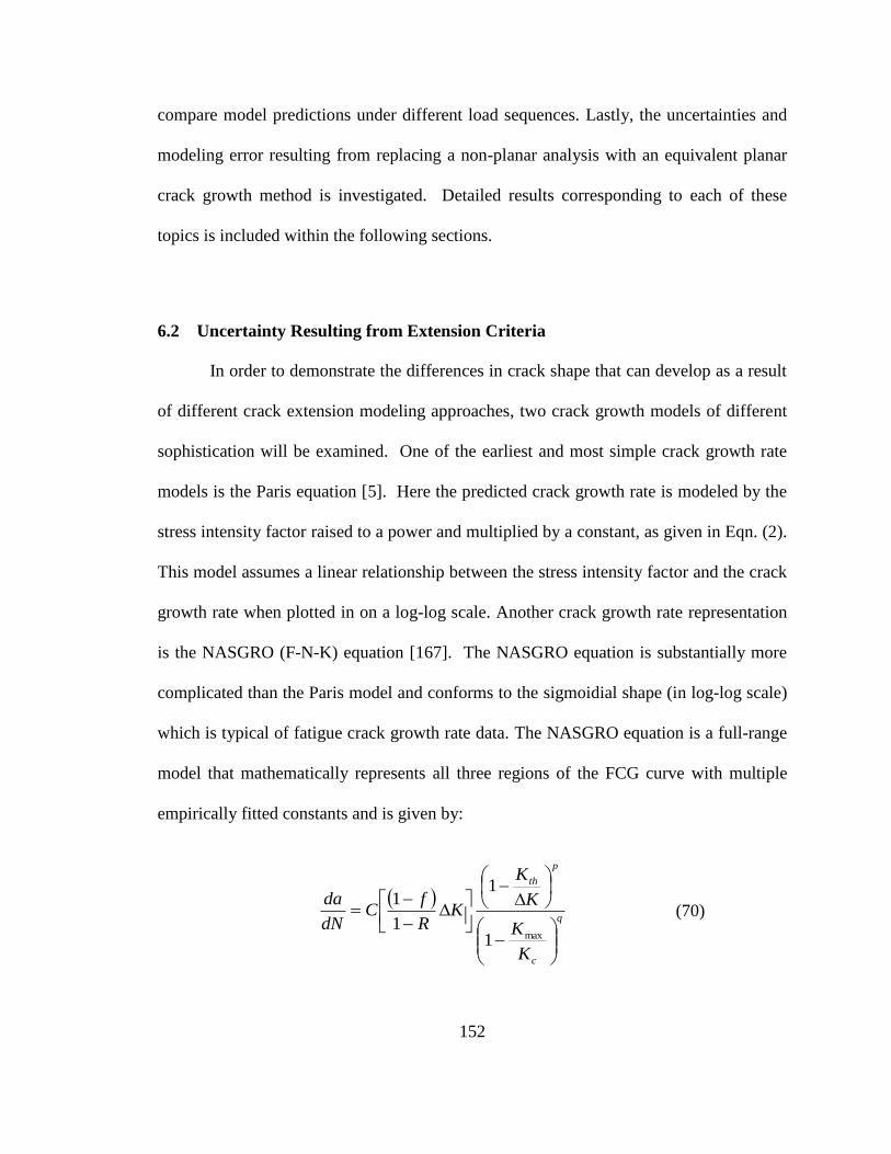
152
compare model predictions under different load sequences. Lastly, the uncertainties and
modeling error resulting from replacing a non-planar analysis with an equivalent planar
crack growth method is investigated. Detailed results corresponding to each of these
topics is included within the following sections.
6.2 Uncertainty Resulting from Extension Criteria
In order to demonstrate the differences in crack shape that can develop as a result
of different crack extension modeling approaches, two crack growth models of different
sophistication will be examined. One of the earliest and most simple crack growth rate
models is the Paris equation [5]. Here the predicted crack growth rate is modeled by the
stress intensity factor raised to a power and multiplied by a constant, as given in Eqn. (2).
This model assumes a linear relationship between the stress intensity factor and the crack
growth rate when plotted in on a log-log scale. Another crack growth rate representation
is the NASGRO (F-N-K) equation [167]. The NASGRO equation is substantially more
complicated than the Paris model and conforms to the sigmoidial shape (in log-log scale)
which is typical of fatigue crack growth rate data. The NASGRO equation is a full-range
model that mathematically represents all three regions of the FCG curve with multiple
empirically fitted constants and is given by:
q
c
p
th
K
K
K
K
KR
fC
dN
da
max1
1
1
1
(70)

153
where C and n are empirical parameters describing the linear region of the curve (similar
to the Paris and Walker models) and p and q are empirical constants describing the
curvature in the FCG data that occurs near threshold (Region I) and near instability
(Region III), respectively. ΔKth is the threshold stress intensity factor, Kc is the critical
stress intensity factor (related to the fracture toughness of the material), and the parameter
f corresponds to the crack opening function. Additional details of the model and
associated parameters can be found in ref [167]. These two crack growth rate equations
represent the extremes in terms of crack growth rate model sophistication. Numerical
investigation into the differences observed in fatigue crack profiles and the corresponding
stress intensity factor solutions at various crack growth stages using these two models is
investigated below.
For the numerical study, the load history consisted of two block variable
amplitude loading conditions where both bending and torsion were applied to the
structure. The crack extension criterion was set to the mean extension criteria for both
simulations. The initial flaw was set as a semi-circular surface flaw within the fillet
radius region of the rotorcraft mast component. The initial flaw half length (c) and depth
(a) were set to 0.05 inches. 12 individual crack growth increments with a median
extension length of 0.01 inches were performed under alternating loading. Within the
simulation, crack extension at each node along the crack front was evaluated for each
growth increment using 2D plane strain approach outlined in Chapter 5. The results of the
analysis can be seen in Figure 51 and Figure 52 the crack front profiles obtained using
the Paris and NASGRO crack growth model are given. In order to improve the
readability of the plots, only the initial crack front and the crack fronts obtained after 6
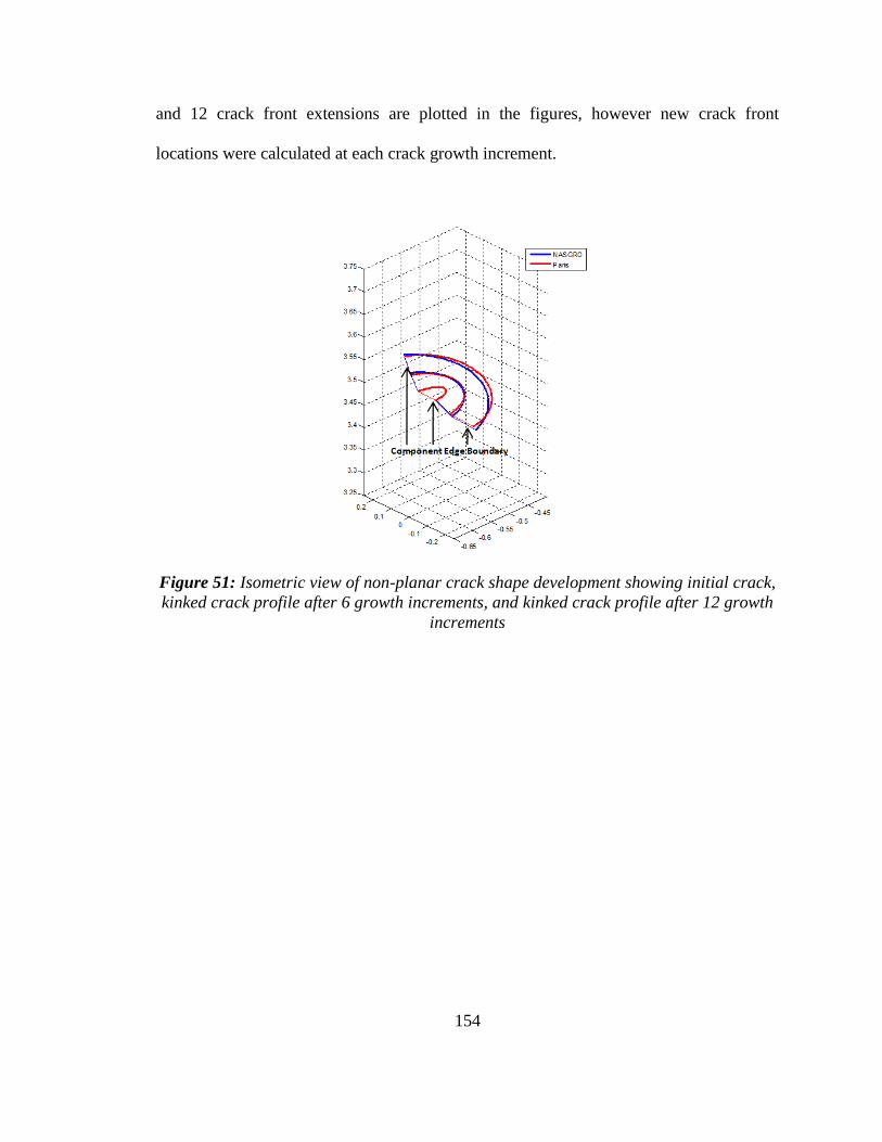
154
and 12 crack front extensions are plotted in the figures, however new crack front
locations were calculated at each crack growth increment.
Figure 51: Isometric view of non-planar crack shape development showing initial crack,
kinked crack profile after 6 growth increments, and kinked crack profile after 12 growth
increments

155
a.) b.)
Figure 52: a.) Plan and b.) Elevation view of non-planar crack shape development
showing initial crack, kinked crack profile after 6 growth increments, and kinked crack
profile after 12 growth increments (showing same crack profiles as Figure 51)
It can be seen that the crack front profiles obtained from using the Paris and
NASGRO crack growth models differs slightly. When compared, the Paris extension
model appears to predict slightly larger crack growth in the crack depth position, and
slightly less crack growth at the free surface of the cylinder. Additionally, at the free
surface of the cylinder the crack edge predicted by the NASGRO equation appears to
have a slightly larger kink angle after several crack growth steps have been made. The
apparent difference in crack kink angle at the later stages of crack growth (clearly
observable after the 6th
crack growth increment) can be attributed to the differences in
crack length at the surface locations. Using the NASGRO extension method, the crack
length at the free surface is seen to be larger than that predicted by the Paris model after
the 6th
growth increment has been performed. This phenomenon can be seen within
Figure 52 b.) where the crack length predicted by the Paris model is ~+/- 0.11 and by
NASGRO is ~+/- 0.125 and the predicted crack kink angles have remained consistent for

156
both methods up to that point. As a result of the noticeable increase in crack length
predicted by the NASGRO equation, the crack profiles predicted by each method at this
crack growth stage are slightly different. The different crack profiles result in different
stress gradients at the crack tip (during the subsequent load cycle), and the crack growth
increment and direction prediction for the following crack growth stages will be different
for each model.
This numerical simulation clearly shows how the use of different fatigue crack
growth extension criterion can not only affect the predicted crack lengths, but also the
predicted crack path. Different criterion will predict slightly different extensions at
different points along the crack front, which will affect the stress gradient and SIF
solution at the following load step, which will again affect the direction and extension
predictions. As a result, it is clear that crack shape development under non-planar crack
growth modeling is dependent on both the crack extension and crack direction criteria
used.
6.3 Uncertainty Resulting from Direction Criteria
Several common crack direction modeling criteria are evaluated within the non-
planar crack growth framework; these include the maximum tangential stress (MTS)
criterion, maximum shear stress (MSS) criterion, and the modified strain energy release
rate (MSERR) criterion. A transition from the maximum tangential stress criterion to the
maximum shear stress (MSS) criterion can be performed by considering the mode I and
mode II fracture toughness material properties. Each of these non-planar crack direction

157
criteria presents a unique solution to the non-planar fatigue crack growth modeling
analysis. Therefore, this analysis produces three unique crack profiles that can be
compared at each crack propagation step. These three direction criteria are chosen for
numerical evaluation since they can be evaluated within the FRANC3D/NG code, as well
as for the familiarity of the general fatigue community with their functional forms.
For the general mixed mode I+II+III condition, the maximum tangential stress
criteria considering tensile only, and tensile + shear (MTSMSS), is given by Eqn. (65),
Eqn. (66), respectively and the modified strain energy release rate criterion is given by
Eqn. (67). For the numerical study, the load history consisted of two block variable
amplitude loading conditions wherein both bending and torsion were applied to the
structure. The crack extension criterion was set to the mean extension criteria for all
simulations. The results of the analysis can be seen in Figure 53 a. & b. where the crack
front profiles obtained using the three different crack direction modeling criteria are
compared. Additionally, since crack shape can have an effect on the stress gradient at the
crack front, the stress intensity factors obtained at the same stage in the crack propagation
analysis (same loading, same number of growth cycles) are compared within Figure 54.
If significant differences can be seen in the resulting stress intensity factors, then different
crack growth rates can be expected, and different component life predictions will be seen.

158
Figure 53: Simulated crack profiles using MTS (tensile only), MTS (tensile or shear) and
MSERR criteria for crack kink direction modeling a.) isometric view; b.) plan view
As can be seen within Figure 53, the predicted crack fronts for the three different
methods do not appear to vary significantly from each other. As a result, it is also seen
that the stress intensity factors for each of the simulated cracks also appear consistent.
These results indicate that the crack direction is dominated by the tensile component of
the stress, and that the shear component is not large enough for transition from tensile to
shear dominated crack growth. In other words, the σθθ(θ) component of Eqns. (65), (66)
and (67) dominates the other terms for the loading conditions considered in this
evaluation.
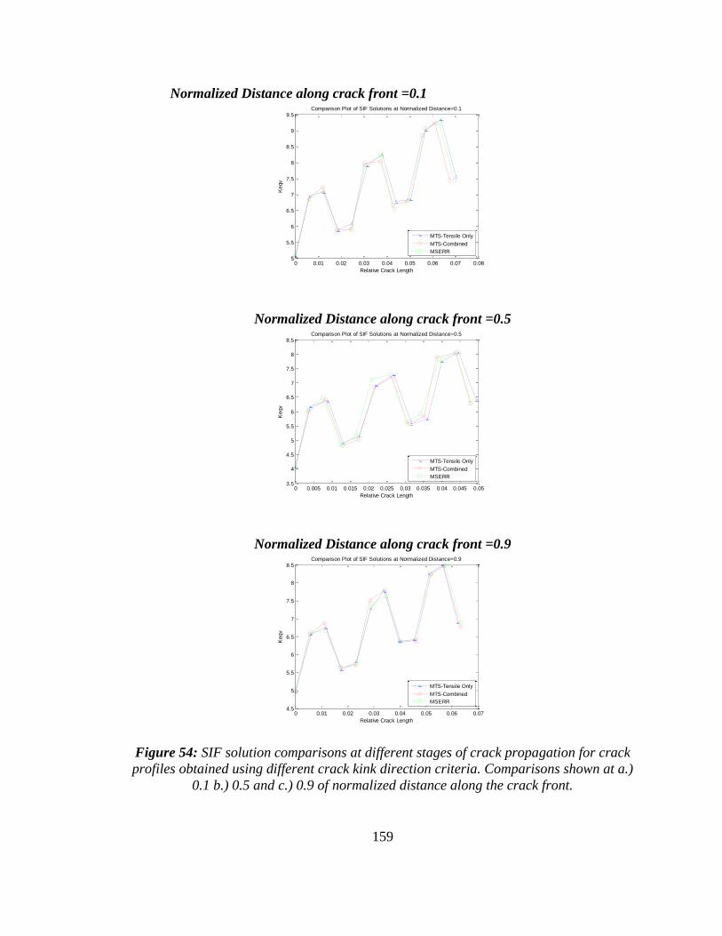
159
Normalized Distance along crack front =0.1
0 0.01 0.02 0.03 0.04 0.05 0.06 0.07 0.085
5.5
6
6.5
7
7.5
8
8.5
9
9.5Comparison Plot of SIF Solutions at Normalized Distance=0.1
Relative Crack Length
Keqv
MTS-Tensile Only
MTS-Combined
MSERR
Normalized Distance along crack front =0.5
0 0.005 0.01 0.015 0.02 0.025 0.03 0.035 0.04 0.045 0.053.5
4
4.5
5
5.5
6
6.5
7
7.5
8
8.5Comparison Plot of SIF Solutions at Normalized Distance=0.5
Relative Crack Length
Keqv
MTS-Tensile Only
MTS-Combined
MSERR
Normalized Distance along crack front =0.9
0 0.01 0.02 0.03 0.04 0.05 0.06 0.074.5
5
5.5
6
6.5
7
7.5
8
8.5Comparison Plot of SIF Solutions at Normalized Distance=0.9
Relative Crack Length
Keqv
MTS-Tensile Only
MTS-Combined
MSERR
Figure 54: SIF solution comparisons at different stages of crack propagation for crack
profiles obtained using different crack kink direction criteria. Comparisons shown at a.)
0.1 b.) 0.5 and c.) 0.9 of normalized distance along the crack front.

160
The applied loading history was modified from that used within the previous
analysis to one that contained more dominant shear loading component (increased torsion
component while decreasing bending). The applied torsion load was increased by a factor
of 2.5 while the bending load did not increase from its previous levels. A similar crack
growth analysis was performed under the new, shear dominated loading conditions to
determine if any significant difference could be observed in the crack shape development.
It can be seen in Figure 55 that under increased shear loading conditions, the maximum
shear stress and the maximum normal stress criteria lead to different crack kinking angles
and crack shape development. The increased torsion load on the component resulted in an
overall increase in the mode III stress intensity factor, which experienced its largest value
along the crack front in the depth direction (0.5 normalized distance along the crack
front). The crack kinking angle predicted by the maximum shearing stress (MSS) criteria
was determined to be smaller than the kink angle predicted by the maximum tangential
stress (MTS) criteria. As evident within the figure, when shear loads cause the mode II
and mode III stress intensity factors to be of the same order as the mode I stress intensity
factor, the crack kinking angle predicted using the MTS and MSS criteria may be
different. As a result, the crack shape development is expected to differ after several
crack growth increments.
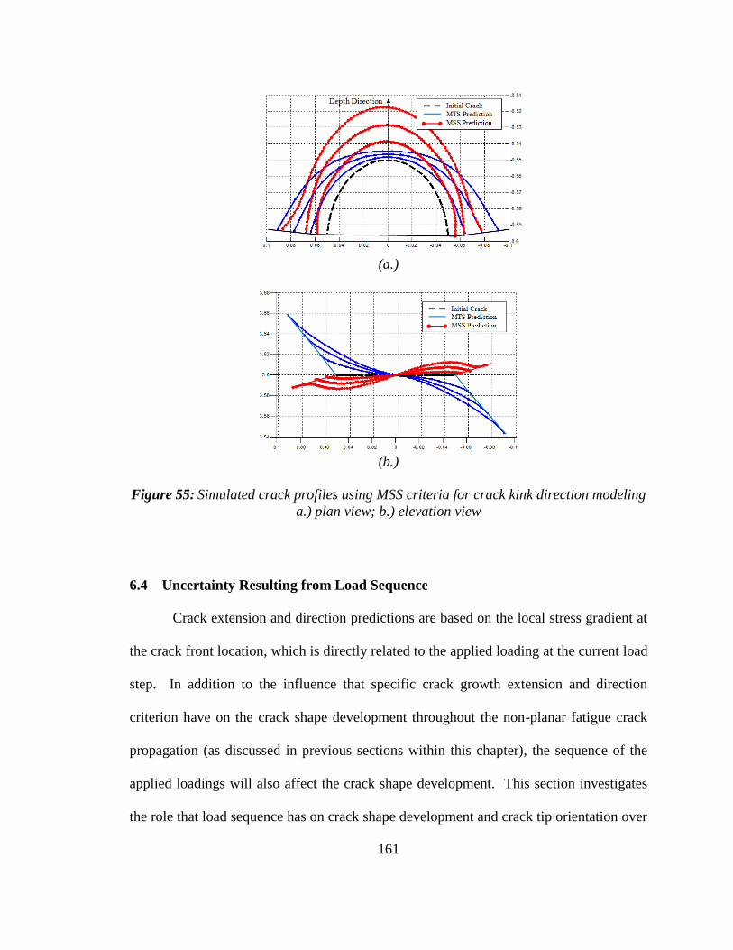
161
(a.)
(b.)
Figure 55: Simulated crack profiles using MSS criteria for crack kink direction modeling
a.) plan view; b.) elevation view
6.4 Uncertainty Resulting from Load Sequence
Crack extension and direction predictions are based on the local stress gradient at
the crack front location, which is directly related to the applied loading at the current load
step. In addition to the influence that specific crack growth extension and direction
criterion have on the crack shape development throughout the non-planar fatigue crack
propagation (as discussed in previous sections within this chapter), the sequence of the
applied loadings will also affect the crack shape development. This section investigates
the role that load sequence has on crack shape development and crack tip orientation over
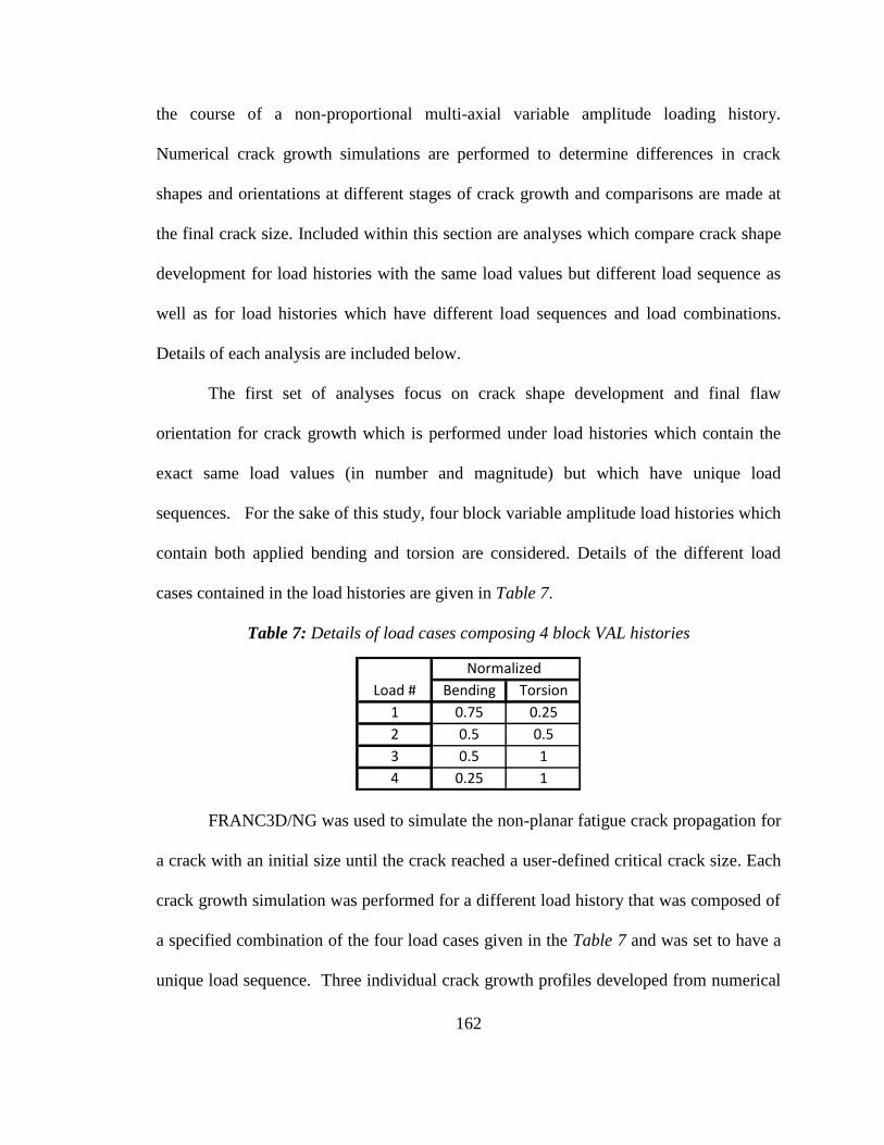
162
the course of a non-proportional multi-axial variable amplitude loading history.
Numerical crack growth simulations are performed to determine differences in crack
shapes and orientations at different stages of crack growth and comparisons are made at
the final crack size. Included within this section are analyses which compare crack shape
development for load histories with the same load values but different load sequence as
well as for load histories which have different load sequences and load combinations.
Details of each analysis are included below.
The first set of analyses focus on crack shape development and final flaw
orientation for crack growth which is performed under load histories which contain the
exact same load values (in number and magnitude) but which have unique load
sequences. For the sake of this study, four block variable amplitude load histories which
contain both applied bending and torsion are considered. Details of the different load
cases contained in the load histories are given in Table 7.
Table 7: Details of load cases composing 4 block VAL histories
Normalized
Load # Bending Torsion
1 0.75 0.25
2 0.5 0.5
3 0.5 1
4 0.25 1
FRANC3D/NG was used to simulate the non-planar fatigue crack propagation for
a crack with an initial size until the crack reached a user-defined critical crack size. Each
crack growth simulation was performed for a different load history that was composed of
a specified combination of the four load cases given in the Table 7 and was set to have a
unique load sequence. Three individual crack growth profiles developed from numerical

163
simulation can be seen within Figure 56. Crack kinking behavior was predicted using the
MTS criterion, and an initial horizontal oriented crack was allowed to grow in a non-
planar fashion at each applied load step. It is seen that the crack shape development is
dependent on the applied loading conditions and that each load sequence results in a
unique crack shape and crack tip orientation at each stage of the crack growth analysis.
-0.2 -0.15 -0.1 -0.05 0 0.05 0.1 0.153.56
3.57
3.58
3.59
3.6
3.61
3.62
3.63
3.64
3.65
Seq 1
Seq 2
Seq 3
(a.)
-0.16 -0.14 -0.12 -0.1 -0.08 -0.06 -0.043.56
3.565
3.57
3.575
3.58
3.585
3.59
3.595
3.6
3.605
Seq 1
Seq 2
Seq 3
(b.)
Figure 56: a.) Full crack; b.) crack tip “A” surface profiles obtained from numerical
simulation showing crack shape development for 3 distinct load sequences under 4 block
variable amplitude loading conditions
Although each individual load sequence was seen to cause a unique crack front
orientation at each crack growth increment, it was found that the crack tip location after
Tip A
Tip B
Crack Growth
Direction

164
application of all of the load steps was similar for all three of the numerical simulations.
This result can be seen within Figure 56 within the lower left hand side of the figure and
indicates that although the individual crack orientations at each crack growth increment
may be different, the combination of all of individual crack kinks result in a similar
overall crack front location. This conclusion is dependent on the fact that each load
history contained exactly the same number and magnitude of applied loading and is based
on the simulation results obtained using the incremental crack growth methodology
detailed in Chapter 5. Based on these results, it appears that the load sequence affects the
crack shape development for interim crack growth stages, but ultimately will not
significantly change the final crack tip location if the number and magnitude of applied
loadings remains consistent from one history to another.
The next set of analyses focus on the differences in crack shape development
under load histories which contain different combinations of the loads contained in Table
7 and which also have which have unique load sequences. This numerical study differs
from the previous case by allowing each load history to contain any combination and any
sequence of the four load cases (whereas the previous study required the same
combination of loads). Crack growth simulation was performed in a similar manner
using the incremental crack growth method and MTS criterion where an initial horizontal
crack was grown to a user-defined critical crack length for each unique load history.
Individual crack growth profiles developed from numerical simulations can be
seen within Figure 57 for this analysis. Similar to the results within the previous
analysis, it is again seen that the crack shape development is dependent on the applied
loading conditions and that each load sequence results in a unique crack shape and crack

165
tip orientation at different stages of the crack growth analysis. However, since each load
history is composed of different combinations of the loading values given in Table 7, the
crack tip locations at the conclusion of the analysis differ from one another. This is the
result of some histories containing a larger number of loadings which are bending
dominated (load case #1 in Table 7) which leads to a less severe crack kinking angle, and
some histories containing a larger number of loading which are torsion dominated (load
case #4 in Table 7) which leads to a more severe crack kinking angle.
-0.2 -0.15 -0.1 -0.05 0 0.05 0.1 0.153.54
3.56
3.58
3.6
3.62
3.64
3.66
Seq 1
Seq 2
Seq 3
Seq 4
Seq 5
Seq 6
(a.)
-0.16 -0.14 -0.12 -0.1 -0.08 -0.06
3.55
3.56
3.57
3.58
3.59
3.6
Seq 1
Seq 2
Seq 3
Seq 4
Seq 5
Seq 6
(b.)
Figure 57: a.) Full crack; b.) crack tip “A” surface profiles obtained from numerical
simulation showing crack shape development for 3 distinct load histories with different
loads and sequences under 4 block variable amplitude loading conditions
Tip A
Tip B
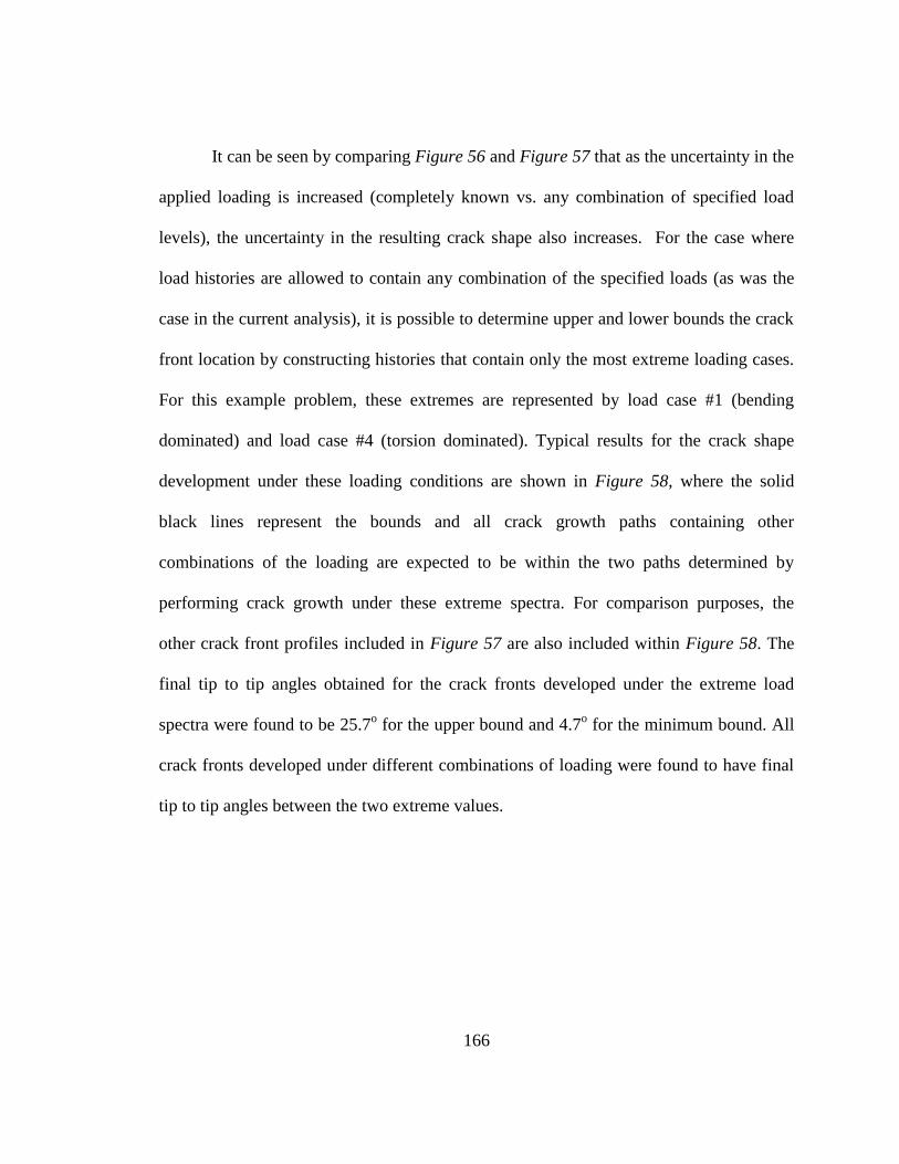
166
It can be seen by comparing Figure 56 and Figure 57 that as the uncertainty in the
applied loading is increased (completely known vs. any combination of specified load
levels), the uncertainty in the resulting crack shape also increases. For the case where
load histories are allowed to contain any combination of the specified loads (as was the
case in the current analysis), it is possible to determine upper and lower bounds the crack
front location by constructing histories that contain only the most extreme loading cases.
For this example problem, these extremes are represented by load case #1 (bending
dominated) and load case #4 (torsion dominated). Typical results for the crack shape
development under these loading conditions are shown in Figure 58, where the solid
black lines represent the bounds and all crack growth paths containing other
combinations of the loading are expected to be within the two paths determined by
performing crack growth under these extreme spectra. For comparison purposes, the
other crack front profiles included in Figure 57 are also included within Figure 58. The
final tip to tip angles obtained for the crack fronts developed under the extreme load
spectra were found to be 25.7o for the upper bound and 4.7
o for the minimum bound. All
crack fronts developed under different combinations of loading were found to have final
tip to tip angles between the two extreme values.

167
-0.2 -0.15 -0.1 -0.05 0 0.05 0.1 0.153.52
3.54
3.56
3.58
3.6
3.62
3.64
3.66
3.68
3.7
Seq 1
Seq 2
Seq 3
Seq 4
Seq 5
Seq 6
Lower Bound
Upper Bound
Figure 58: Upper and lower bounds on crack front paths determined by performing
crack growth simulation under extreme load histories
Through several numerical crack growth studies, it is shown that the sequence of
the applied loadings can have a significant effect on the crack shape development over
time. For the most general case, where possible load histories can only be characterized
by the load levels (without any indication of how frequent each load level is or how often
it is encountered), non-planar crack shapes may significantly deviate from one another
depending on the combination of loads contained within each history. However, it is
possible to determine the upper and lower bounds on the crack front location by
identifying the loading cases which cause the most severe (largest and smallest) kink
angles, and performing non-planar analysis using load histories containing only these
values. As additional information is available on the expected frequency of each load
level within the load history, less scatter is expected in the crack path predictions made
under different load sequences. It was found that for the limiting case where each history
is composed of loads which differ only in the sequence and not the magnitude or
number/frequency of each applied load, the crack path differed during each crack growth
168
increment but converged to the same general location after all crack growth steps had
been performed. Overall, it was determined that loading and load sequence can have a
significant effect on the crack shape development when considering non-planar crack
growth under variable amplitude, multi-axial loading conditions, and that uncertainty in
the characterization of the applied loads results in increased uncertainty in the non-planar
crack profile.
6.5 Non-Planar vs. Equivalent Planar Comparison
An equivalent planar crack growth modeling strategy has been presented in
Chapter 5, which proposes the use of an equivalent planar crack, which can be
characterized by various features extracted from the initial non-planar result, as an
approximate representation of the more sophisticated non-planar approach. Errors will
exist in the equivalent planar representation when compared to the original non-planar
result as a result of these simplifications. These errors need to be quantified in order to be
able to estimate the uncertainty in model predictions using the equivalent planar
modeling approach.
This section will examine the crack growth modeling results for crack growth
simulations using the equivalent planar method. The first investigation will use a simple
constant amplitude loading condition (in both bending and torsion) to investigate the case
where a single crack kink angle is expected. The second investigation will consider a two
block loading condition where multiple crack kinking angles are expected. The final
investigation will analyze the equivalent planar approximation under the four block load
169
history where load sequence effects are also considered. The initial crack size and
location within the component remain the same as previous studies. The result of the
analyses is included below.
The first comparison of the accuracy of the equivalent planar method in
representing the non-planar crack growth modeling considered the simplest loading case,
where only constant amplitude bending and torsion loading are applied. For this specific
analysis, the applied loading was set to load level #3 in Table 7. Figure 59 a) b) and c)
show comparison plots at different normalized distances around the crack front (0.1, 0.5,
and 0.9 respectively) of the stress intensity factor results at various stages of crack growth
for the non-planar and equivalent planar simulations under the constant amplitude
bending + torsion loading conditions. For the constant amplitude load case only one
primary kink angle is expected, resulting in the equivalent planar crack to be oriented
directly at this kink angle. As seen in the plots, the planar representation is able to
closely match those found using the non-planar crack methodology for this load case, as
might be expected. The percent error between the equivalent planar and the non-planar
analysis at any location along the crack front is found to be less than 15% at all stages of
crack growth, and less than 6% for all stages after the initial crack growth increment,
with an overall absolute mean error of 3.7%.

170
0.05 0.1 0.15 0.2 0.25 0.3 0.35 0.45
10
15
Crack Front Length (in)
De
lta
K e
qv
SIF vs. Crack Length for CAL case( Normalized 0.1 crack front location)
Nonplanar - Load 1
Fit
Planar - Load 1
Fit
(a.)
0.05 0.1 0.15 0.2 0.25 0.3
4
5
6
7
8
9
10
11
Crack Front Length (in)
De
lta
K e
qv
SIF vs. Crack Length for CAL case( Normalized 0.5 crack front location)
Nonplanar - Load 1
Fit
Planar - Load 1
Fit
(b.)
0.05 0.1 0.15 0.2 0.25 0.3 0.35 0.45
10
15
Crack Front Length (in)
De
lta
K e
qv
SIF vs. Crack Length for CAL case( Normalized 0.9 crack front location)
Nonplanar - Load 1
Fit
Planar - Load 1
Fit
(c.)
Figure 59: Comparison plots of stress intensity factor solutions found using non-
planar crack growth methodology and equivalent planar crack growth methodology for
CAL load case. Plots show SIFs along the crack front at a.) 0.1 normalized distance
(near surface); b.) 0.5 normalized distance (depth); c.) 0.9 normalized distance (near
surface)

171
The second comparison of the accuracy of the equivalent planar method in
representing the non-planar crack growth modeling considered a two block variable
amplitude loading case, where both bending and torsion loading are applied. For this
specific analysis, the applied loading was restricted to load level #1 and load level #3 in
Table 7. Figure 60 a) b) and c) show comparison plots at different normalized distances
around the crack front (0.1, 0.5, and 0.9 respectively) of the stress intensity factor results
at various stages of crack growth for the non-planar and equivalent planar simulations
under the 2 block variable amplitude bending + torsion loading condition. Under the
two-block loading case, two distinct kink angles are to be expected resulting in a zigzag
type crack edge profile (as seen in Figure 49), and the resulting equivalent planar crack
orientation essential becomes the average kink angle of the two loading conditions.
As seen from the plots, the planar representation is also able to closely match
those found using the non-planar crack methodology for this 2 block load case. The
largest discrepancy between the two results is seen during the first growth stage. At this
point in the simulation, the two configurations are the most different as the crack has an
initial orientation of 0o for the non-planar crack growth before kinking, and ~17
o in the
case of planar crack growth. This large difference in orientation was found to effectively
reduce the magnitude of both the mode II and III stress intensity factors for the planar
analysis at the surface locations (as opposed to depth location), thus lowering the overall
ΔKeqv value for this crack size. However, after several crack growth steps, it is found that
the planar approximation more closely matched that of the non-planar analysis. The
percent error between the equivalent planar and the non-planar analysis are found to be

172
less than 18% at all stages of crack growth, and less than 7% for all stages after the initial
crack growth increment, with an overall absolute mean error of 2.9%.
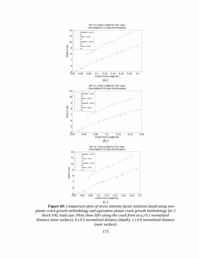
173
0.04 0.06 0.08 0.1 0.12 0.14 0.16 0.18 0.25
6
7
8
9
10
11
12
Crack Front Length (in)
De
lta
K e
qv
SIF vs. Crack Length for CAL case( Normalized 0.1 crack front location)
Nonplanar - Load 1
Fit
Planar - Load 1
Fit
Nonplanar - Load 2
Fit
Planar - Load 2
Fit
(a.)
0.04 0.06 0.08 0.1 0.12 0.14 0.164
5
6
7
8
9
10
11
Crack Front Length (in)
De
lta
K e
qv
SIF vs. Crack Length for CAL case( Normalized 0.5 crack front location)
Nonplanar - Load 1
Fit
Planar - Load 1
Fit
Nonplanar - Load 2
Fit
Planar - Load 2
Fit
(b.)
0.04 0.06 0.08 0.1 0.12 0.14 0.16 0.18 0.25
6
7
8
9
10
11
12
Crack Front Length (in)
De
lta
K e
qv
SIF vs. Crack Length for CAL case( Normalized 0.9 crack front location)
Nonplanar - Load 1
Fit
Planar - Load 1
Fit
Nonplanar - Load 2
Fit
Planar - Load 2
Fit
(c.)
Figure 60: Comparison plots of stress intensity factor solutions found using non-
planar crack growth methodology and equivalent planar crack growth methodology for 2
block VAL load case. Plots show SIFs along the crack front at a.) 0.1 normalized
distance (near surface); b.) 0.5 normalized distance (depth); c.) 0.9 normalized distance
(near surface)

174
The final analysis of the equivalent planar method considers the four block
variable amplitude loading case wherein the load sequence is flexible. The three unique
non-planar crack growth results obtained from previous analyses in Section 6.4 (and
shown in Figure 56) are used to show how multiple non-planar crack growth results can
be combined for a single equivalent planar crack analysis. Three different load histories
(composed of the same loading values, but with different sequences) were used to
perform non-planar crack growth simulations. The final angle of orientation between the
crack tips at the surface locations was determined using the method detailed in Section
5.5 for each simulation result. For the three cracks shown in Figure 56 corresponding to
the three different load sequences, the angles of the equivalent flaw size were determined
to be 13.18, 13.50, and 13.95 degrees. The orientation of the equivalent planar crack was
set to be the average value obtained from the three individual results and planar crack
growth analysis was performed and results compared. Figure 61 a), b), and c) show
comparison plots at different normalized distances around the crack front (0.1, 0.5, and
0.9 respectively) of the stress intensity factor results at various stages of crack growth for
the non-planar and average equivalent planar simulation for the 4 block variable
amplitude history. Plots showing similar results are obtained when the stress intensity
factors obtained from the average equivalent planar results are compared to those from
the non-planar for other load histories.

175
0.04 0.06 0.08 0.1 0.12 0.14 0.163
4
5
6
7
8
9
10
Crack Front Length (in)
De
lta
K e
qv
SIF vs. Crack Length for 4 Block VAL case( Normalized 0.1 crack front location)
Nonplanar - Load 1
Planar - Load 1
Nonplanar - Load 2
Planar - Load 2
Nonplanar - Load 3
Planar - Load 3
Nonplanar - Load 4
Planar - Load 4
(a.)
0.05 0.06 0.07 0.08 0.09 0.1 0.11 0.12 0.132
3
4
5
6
7
8
9
Crack Front Length (in)
De
lta
K e
qv
SIF vs. Crack Length for 4 Block VAL case( Normalized 0.5 crack front location)
Nonplanar - Load 1
Planar - Load 1
Nonplanar - Load 2
Planar - Load 2
Nonplanar - Load 3
Planar - Load 3
Nonplanar - Load 4
Planar - Load 4
(b.)
0.04 0.06 0.08 0.1 0.12 0.143
4
5
6
7
8
9
Crack Front Length (in)
De
lta
K e
qv
SIF vs. Crack Length for 4 block VAL case( Normalized 0.9 crack front location)
Nonplanar - Load 1
Planar - Load 1
Nonplanar - Load 2
Planar - Load 2
Nonplanar - Load 3
Planar - Load 3
Nonplanar - Load 4
Planar - Load 4
(c.)
Figure 61: Comparison plots of stress intensity factor solutions found using non-
planar crack growth methodology and equivalent planar crack growth methodology for 2
block VAL load case. Plots show SIFs along the crack front at a.) 0.1 normalized
distance (near surface); b.) 0.5 normalized distance (depth); c.) 0.9 normalized distance
(near surface)

176
For the more general load case where the exact combination of applied loadings
contained within a load history is not precisely known, the orientation of the final non-
planar crack has been shown to be dependent on both the applied load values and the
sequence in which they are applied. This makes it difficult to accurately predict the final
orientation of the fatigue crack without a full non-planar analysis for a specific load
history. As a result, the need for an efficient and accurate method for non-planar crack
shape development is desired to be able to predict the final crack orientation under unique
load histories. This topic remains an open area of research and would enable a broader
applicability to the current equivalent planar methodology by providing final flaw
orientations without the expensive task of component stress and crack growth analysis.
Overall, the equivalent planar crack growth modeling approach appears to provide
a reasonable approximation to the non-planar crack growth analysis. Comparative results
are included for simple constant amplitude, two-block, and four-block variable amplitude
load histories. Errors in the stress intensity factors at similar stages of crack growth
resulting from the simplification to a planar crack representation were found to be
anywhere from 5-20% for the cases considered. The equivalent planar method reduces
the necessary computational effort and complex crack shape characterization by using the
results from a non-planar analysis and effectively reducing them onto a single plane
orientation. In doing so, this method reduces the complex non-planar crack growth
problem to a planar type problem which can be effectively modeled using techniques
developed in the previous chapters of this dissertation.

177
6.6 Summary
Non-planar crack kinking behavior significantly increases the complexity of both
the analytical models and the computational modeling demands. Since non-planar crack
growth modeling requires both crack extension and crack direction predictions and no
universal theory exists, uncertainties are introduced into the model predictions resulting
from the use of different non-planar crack growth criteria. The choice of crack extension
and direction modeling criteria has an influence on crack shape, the stress gradient at the
crack tip, and the overall predicted fatigue life. The use of different criteria may result in
differences in fatigue crack growth model predictions and the differences between the
various methods will be problem specific. It is important that crack growth model
predictions to compare mode predictions to experimental and in-service physical
specimens whenever possible.
Since non-planar crack growth is an incremental process where the crack shape
development is dependent on previous crack growth predictions, the sequence and
magnitude of applied loads may have an effect on the final crack size, shape, and
orientation within the structural component. Uncertainty in the composition of loading
values contained within a load history as well as loading sequence has been shown to
have an effect on the crack shape development under multiaxial variable amplitude
loading conditions. However, it is possible to determine upper and lower bounds on the
crack tip orientation under different load combinations by performing non-planar analysis
for extreme load spectra.
This chapter also investigated the uncertainty in stress intensity factor solutions
and crack growth predictions using an equivalent planar crack growth modeling approach

178
in place of a more computationally demanding non-planar analysis. The equivalent planar
method appears to provide reasonable approximations for most crack configurations and
load combinations where a full non-planar analysis is possible and has been investigated
under constant amplitude as well as variable amplitude block type loading conditions.

179
CHAPTER VII
SUMMARY & FUTURE WORK
7.1 Summary
The traditional damage tolerance (DT) approach to aircraft structures has assumed
a deterministic damage accumulation process where deterministic crack growth curves,
constant material properties, and specific initial flaw sizes are used. However,
uncertainties exist at all levels of the fatigue damage tolerance modeling process,
resulting in unknown confidence bounds on component life predictions made by
engineers. In order to overcome this limitation, a systematic framework for stochastic
fatigue crack growth modeling must be developed which accounts for different kinds and
sources uncertainty that exist at all levels of the damage tolerance analysis. Each
individual source of uncertainty, resulting from physical variability, data uncertainty, or
modeling errors, needs to be identified and its statistical characteristics quantified in
order to accurately assess the risk of failure of structural components. It is the goal of
this dissertation to provide a methodical and practical framework for quantifying various
sources of uncertainty and analyzing their effects on component reliability predictions
over time.
The first several chapters of this work focus on uncertainty quantification,
probabilistic fatigue crack growth modeling, and model error assessment for planar crack
growth analysis. This research provides methods for uncertainty quantification of many
fundamental material properties which are important to fatigue crack growth, such as the

180
threshold stress intensity factor and the fatigue limit, with particular attention focused on
accurately representing the near threshold and linear (Paris) regions of the crack growth
rate curve which are important to the high cycle fatigue problem. As each additional
model within the fatigue crack growth analysis framework is used to represent the crack
propagation, additional uncertainties are introduced into the model predictions as a result
of model form errors. This research focuses on quantifying the statistical uncertainty in
each model prediction to more accurately represent the overall uncertainty in component
fatigue life predictions. Included in this area are topics ranging from uncertainty in
fatigue crack growth rate model representation, finite element discretization errors, and
uncertainty in surrogate model predictions. Each of these individual sources of modeling
uncertainty needs to be represented in different ways, and this work provides a
methodical approach for accurate quantification and inclusion within an overall
probabilistic fatigue life assessment.
The latter half of this dissertation shifts focus to identify additional sources of
uncertainty which are introduced when non-planar fatigue crack growth modeling is
performed. When considering non-planar crack growth modeling, it is important to be
able to predict and model both the crack extension magnitude and the crack path
direction. This leads to an increase in the complexity of crack shape representation as
well as computational modeling considerations. In order to try to capture the nonlinear
crack extension behavior that has been seen in both experimental results and realistic
applications, numerous crack growth direction and extension criteria have been proposed
within the literature. However, to date no single criteria has been identified as a
universally applicable model. This research investigates the differences in fatigue crack

181
shape development and fatigue life predictions which result from the use of different
crack extension and direction modeling criteria. It is seen through numerical simulation
results that the choices of both the extension and direction criteria can have an effect on
the crack shape development of fatigue cracks growing under multiaxial variable
amplitude loading conditions. Since crack growth analysis is an incremental process,
where subsequent crack growth steps are directly dependent on previous crack growth
steps (through the stress gradient at the crack tip), small differences in crack orientation
and crack extension at each growth step can lead to different crack shape representations
after a finite number of crack growth increments.
An equivalent planar crack representation method is developed within this work
to try to utilize the information obtained about the crack shape development and final
crack orientation from the more sophisticated non-planar analysis, while enabling the use
of simpler crack representation and modeling approach afforded by the planar
representation. The method proposes to utilize a finite number of non-planar crack
growth analyses to characterize the non-planar crack shape development under multiaxial
variable amplitude loading conditions. The orientation of the final crack shape is then
used to determine a suitable angle of orientation of an initial crack within the component
that can be used within a planar crack growth analysis procedure. The equivalent planar
representation is an approximation to the more realistic non-planar crack growth method,
but appears to provide reasonable results when compared to full non-planar analyses for
constant amplitude and multiple block variable amplitude histories.
Overall, this dissertation systematically identifies, quantifies, and incorporates
different types of uncertainties within an overall probabilistic life prediction modeling

182
approach. The uncertainty quantification (UQ) methodology is implemented with 3-
dimensional planar and non-planar fatigue crack modeling, for structural components
subjected to multi-axial, variable amplitude loading conditions. Included within the
scope of this work are UQ methods for material properties and model parameters, as well
as methods which focus on model error quantification – including FEA discretization
error and surrogate modeling error. Additionally, the uncertainty quantification and
propagation methodology is developed to be computationally efficient to enable the
component reliability assessment to be performed within a Monte Carlo Scheme.
Sensitivity analysis is presented to identify the contribution that each source of
uncertainty has on the overall component life prediction.
Some of the key contributions contained within this work include:
Extended stochastic field expansion technique to fatigue crack propagation
modeling, which enables a more realistic representation of the correlation among
the fatigue crack growth rate test data
New framework for PFM enabling fatigue crack growth modeling under multi-
axial, variable amplitude loading conditions incorporating FEA, characteristic
plane, surrogate model, and cyclic crack growth modeling methods
Developed new application of Gaussian Process surrogate modeling technique for
mixed mode SIF evaluation under multi-axial loading for improved computational
efficiency
Implemented new technique for identifying critical input parameter combinations
that help reduce uncertainty in the training point selection for the design of
experiments (DOE) of the full model FEA
183
Quantified and incorporated finite element discretization modeling errors within
component fatigue life assessment framework
Quantified and incorporated surrogate modeling (response surface) modeling errors
within component fatigue life assessment framework
Proposed an „equivalent planar‟ fatigue crack growth modeling approach to reduce
the computational expense of numerical simulations while retaining valuable
features of a full scale non-planar crack growth analysis
Quantified uncertainty in crack shape and stress intensity factor solutions resulting
from use of different crack extension criteria for non-planar crack growth
modeling
Quantified uncertainty in crack shape and stress intensity factor solutions resulting
from use of different crack direction criteria for non-planar crack growth
modeling
Evaluated model errors for an „equivalent planar‟ fatigue crack growth modeling
approach compared to traditional non-planar results
7.2 Future Research Needs
This study implemented fatigue crack growth analysis using both planar and non-
planar fatigue crack growth modeling techniques. While the area of planar crack growth
under constant amplitude and variable amplitude loading has been well documented
within the fatigue research community, non-planar crack growth modeling, particularly in
three dimensions, is a more recent area of interest. From a theoretical point of view,

184
continued research is necessary on developing a universal fatigue crack growth extension
and direction criteria. Currently, many different criteria exist, and different researchers
argue as to the appropriateness of each under different loading conditions and in
reference to different experimental results. In order to develop a universal criteria that is
widely applicable to different load conditions, it is necessary to increase the current
physical understanding of fatigue crack growth mechanisms under multiaxial loads.
Efforts are underway to increase experimental testing under multi-axial loads for
different materials, where only simple uniaxial tensile load cases have previously been
performed. However, one current limitation which makes direct comparison and data
transfer possible difficult is the lack of a standardized and detailed multiaxial testing
procedure and standard test specimen. As a result, results obtained from different sources
and researchers tend to use different testing procedures on a wide range of test specimen
which raises the question of whether differences seen in the results for mixed mode
fatigue crack growth properties are the result of natural variability or whether they are
simply the product of different testing methods. Further research in this area is necessary
before a meaningful and thorough database of mixed mode material properties can be
built.
Surrogate modeling techniques were implemented within the planar fatigue crack
growth analysis to efficiently capture the relationship between the crack shape, size, and
current loading conditions and the stress intensity factors along the crack tip. Within the
non-planar crack growth analysis procedure, the development of a similar method is
much more involved as a result of the complexity in crack shape representation and the
interdependence between the previous loads and the crack shape development. A

185
promising area of future research exists in developing an efficient and accurate method
for three dimensional non-planar crack shape predictions. New methods must be
developed which address the issue of how to best represent the complex, non-planar three
dimensional crack surface. Any surrogate modeling technique must also be able to
capture the direct relationship that exists between the previous applied load sequence and
the current crack shape representation. Once developed, these methods will still rely on
accurate non-planar crack growth analysis for training data under multiaxial load
histories. As a result, continued effort and resources should be focused on improved finite
element models, remeshing algorithms, increased computational efficiency, and more
robust crack growth modeling capabilities.
Overall, many advanced topics in the fields of fatigue and fracture mechanics for
multiaxial crack growth still exist and are worth pursuing. As new theoretical and
computational methods are developed and proposed, it is necessary that a sufficient
amount of meaningful and representative experimental results are available to compare,
verify, and validate the proposed methods against those which have been previously
developed.

186
REFERENCES
1 R.P. Reed, J.H. Smith, and B.W. Christ, “The economic effects of fracture in the United
States,” SP647-1,NBS, March 1983, 3.
2 A.F. Grandt, Jr., Fundamentals of structural integrity: damage tolerant design and
nondestructive evaluation, John Wiley & Sons, Inc., 2004.
3 Y.C. Tong, Literature review on structural Risk and reliability analysis. Aeronautical
and Maritime Research Laboratory. report DSTO-TR-1110, Melbourne,
Australia, Feb. 2001.
4 FAA, Rotorcraft Damage Tolerance (RCDT) R&D Roadmap for metallic materials.
Airworthiness Assurance Team, FAA, 2006.
5 P.C. Paris, M.P. Gomez, W.E. Anderson, A rational analytic theory of fatigue, The
trend in engineering. University of Washington, 13(1), 1961, pg. 9-14.
6 R. G. Forman, V. E. Kearney, R. M. Engle, Numerical analysis of crack propagation in
cyclic-loaded structures. Journal of Basic Engineering, Trans, ASME, Vol. 89, pp.
459-464, 1967.
7 K. Walker, The effect of stress ratio during crack propagation and fatigue for 2024-T3
and 7075-T6 Aluminum, ASTM STP 462, American Society for Testing and
Materials (Philadelphia), p. 1, 1970.
8 F. Erdogan,M. Ratwani, Fatigue and fracture of cylindrical shells containing a
circumferential crack. International Journal of Fracture Mechanics, 6, 379-392.
9 T.L. Anderson, Flaw Characterization, Comprehensive structural integrity Volumes 1-
10, Edited by: I. Milne, R.O. Ritchie, B. Karihaloo, Elsevier, 2003.
10 A.F. Grandt, Jr. Fundamentals of Structural Integrity: Damage tolerant design and
nondestructive evaluation, John Wiley & Sons, Inc., New Jersey, 2004.
11 J.P. Gallagher, F.J. Glessler, A.P. Berens, USAF Damage Tolerant Design Handbook:
guidelines for the analysis and design of damage tolerant aircraft structures,
AFWAL-TR-82-3073, 1984.
12 X.B. Lin, R.A. Smith, An improved numerical technique for simulating the growth of
planar fatigue cracks, Fatigue Fracture Engineering Materials & Structures, Vol.
20, No. 10, pg 1363-1373, 1997.
13 Y. Liu, S. Mahadevan, Analysis of subsurface crack propagation under rolling contact
loading in railroad wheels using FEM, Engineering Fracture Mechanics, Vol. 74,
pg 2659-2674, 2007.
14 X.B. Lin, R.A. Smith, Fatigue growth simulation for cracks in notched and unnotched
round bars, International Journal of Mechanical Sciences, Vol. 40, No. 5, pg 405-
419,1998.

187
15
P.M. Besuner, Probabilistic fracture mechanics, In: Probabilistic fracture mechanics
and reliability, Ed: J.W. Provan, Martinus Nijhoff Publishers, 1987.
16 S. Rahman, B.N. Rao, Probabilistic fracture mechanics by Galerkin meshless methods
– part II: reliability analysis, Computational Mechanics, Vol. 28, No. 5, May,
2002.
17 C.A. Rau, Jr. P.M. Besuner. Probabilistic fracture mechanics, Product Engineer, Vol.
50, pg 41-47, 1979.
18 M. Shinozuka, J.N. Yang, Optimum structural design based on reliability and proof
load test, Annals of Assurance Science Proceedings of the Reliability and
Maintainability Conference, Vol. 8, July, 1969.
19 J.N. Yang, W.J. Trapp, Reliability analysis of aircraft structures under random loading
and periodic inspection, AIAA Journal, Vol. 12, pg 1623-1639, 1974.
20 H. Alawi, Designing reliably for fatigue crack growth under random loading,
Engineering Fracture Mechanics, Vol. 37, No. 1, pg 75-85, 1990.
21 D.O. Harris, E.Y. Lim, D.D. Dedhia, Probability of pipe fracture in the primary coolant
loop of a PWR plant, Vol. 5, Probabilistic Fracture Mechanics, U.S. Nuclear
Regulatory Commission Report NUREG/CR-2189, 5, Washington D.C., 1981.
22 S.C. Forth, M.A. James, W.M. Johnston, J.C. Newman Jr., Anomalous fatigue crack
growth phenomena in high strength steel, In: Proceedings international congress
on fracture, Italy, 2007.
23 U.H. Tiong, R. Jones, Damage tolerance analysis of a helicopter component,
International Journal of Fatigue, Vol. 31, pg. 1046-1053, 2009
24 B. Ayyub, Uncertainty modeling and analysis in civil engineering, CRC Press LLC,
1998.
25 N.R. Moor, D.H. Ebbeler, and M. Creager, Probabilistic service life assessment, AD-
Vol. 28, Reliability Technology, ASME 1992
26 M.E. Melis, E.V. Zaretsky. Probabilistic analysis of aircraft gas turbine disc life and
reliability, NASA/TM-1999-107436.
27 R.V. Lust, Y.T.J. Wu, Probabilistic structural analysis – an introduction, Experimental
Techniques, September/October 1998.
28 Y. Xiaoming, H.C. Kuang, K.C. Kyung. Probabilistic structural durability prediction,
AIAA Journal, Vol. 36, No. 4, April 1998.
29 T. Svensson, Prediction uncertainties at variable amplitude fatigue. International
Journal of Fatigue, 17, pg 295-302, 1997.

188
30
R. Bullough, V.R. Green, B. Tomkins, R. Wilson, J.B. Wintle, A review of methods
and applications of reliability analysis for structural integrity assessment of UK
nuclear plant. International Journal of Pressure Vessel Piping, Vol. 76, pg 909-
919, 1999.
31 P. Dillström, F. Nilsson, B. Brickstad, and M. Bergman, Probabilistic fracture
mechanics analysis of a nuclear pressure vessel for allocation of in-service
inspection. International Journal of Pressure Vessel Piping, Vol. 54, pg 435-463,
1993.
32 O. Ditlevsen and H.O. Madsen, Structural reliability methods, Wiley, Baffins Lane,
Chichester, pg 372, 1996.
33 F.M. Burdekin, W. Hamour. SINTAP contribution to Task 3.5, Safety factors and risk,
UMIST, pg. 25, 1998.
34 British Energy, Assessment of the integrity of structures containing defects, British
energy generation report R6, revision 4, Gloucester, UK, 2001.
35 L.P. Pook, Metal Fatigue: what it is, why it matters. Springer, 2007.
36 L.P. Pook, The role of crack growth in metal fatigue. Metals Society, London, 1983.
37 J. Backlund, A.F. Blom, C.J. Beevers, Fatigue threshold, fundamentals and engineering
applications, in Proceedings of the International Conference held in Stockholm,
June 1981.
38 M. Klesnil, P. Lukas, Effect of stress cycle asymmetry on fatigue crack growth,
Material Science Engineering, Vol. 9, pg 231-240, 1972.
39 J.M. Barsom, Fatigue behavior of pressure vessels steel, WRC Bulletin 194, Welding
Research Council, New York, May 1964.
40 B. Farahmand, Fatigue and Fracture Mechanics of High Risk Parts, Chapman & Hall,
New York, 1997.
41 A. Haldar, S. Mahadevan, Probability, reliability, and statistical methods in
engineering design, John Wiley & Sons, 2000.
42 F.P. Beer, E.R. Johnston Jr., Mechanics of Materials (2
nd Edition). McGraw-Hill, Inc.
1992.
43 R.C. Rice, J.L. Jackson, J. Bakuckas, S. Thompson. Metallic materials properties
development and standardization (MMPDS), DOT/FAA/AR-MMPDS-01,
January 2003.
44 M. McDonald, K. Zaman, and S. Mahadevan, Representation and First-Order
Approximations for Propagation of Aleatory and Distribution Parameter
Uncertainty. In the Proceedings of 50th AIAA/ASME/ASCE/AHS/ASC
189
Structures, Structural Dynamics, and Materials Conference, 4 - 7 May 2009, Palm
Springs, California.
45 B. Efron, R. Tibshirani. An Introduction to the Bootstrap. New York: McGraw-Hill,
1993.
46 B. Efron, Bootstrap methods: another look at the jackknife, Annals of Statistics, Vol. 7,
No. 1, pg. 1-26, 1979.
47 P. Dillstrom, F. Nilsson, Probabilistic fracture mechanics, In: Comprehensive
Structural Integrity, ED: l Milne, R.O. Ritchie, B. Karihaloo, Elsevier, 2003.
48 J.N. Yang, G.C. Salivar, C.G. Annis Jr., Statistical modeling of fatigue crack growth in
nickel-base superalloy, Engineering Fracture Mechanics, Vol. 18, No. 2, pg. 257-
270, 1983
49 J.W. Provan, Probabilistic Fracture Mechanics and Reliability, Martinus Nijhoff,
Dordrecht, 1987.
50 N.R. Moore, D.H. Ebbeler, S. Sutharshana, M. Creager, Probabilistic failure risk
assessment for structural fatigue, Jet Propulsion Laboratory, 1992.
51 T.A. Cruse, S. Mahadevan, R.G. Tryon, Fatigue reliability of gas turbine engine
structures, NASA/CR-97-206215, Lewis Research Center, 1997.
52 Y. Liu, S. Mahadevan, Stochastic fatigue damage modeling under variable amplitude
loading. International Journal of Fatigue, Vol. 29, pg 1149-1161, 2007.
53 J.N. Yang, S.D. Manning, “A simple second order approximation for stochastic crack
growth analysis”, Engineering Fracture Mechanics, Volume 53, Issue 5, pp. 677-
686, 1996.
54 Z. Zhao, A. Haldar, Bridge fatigue damage evaluation and updating using non-
destructive inspections. Engineering fracture mechanics, Vol. 53, No. 5, Pg 775-
788, 1996.
55 R. Zheng, S. Mahadevan, Model uncertainty and bayesian updating in reliability-based
inspection. Structural Safety Vol. 22, pg 145-160, 2000.
56 T.D. Righiniotis, Simplified calculations involving the maximum load on bridge
fatigue details under inpection. Part II: Fatigue. Journal of Constructional Steel
Research, Vol. 50, pg 825-839, 2004.
57 M. S. Cheung, W.C. Li, “Probabilistic fatigue and fracture analyses of steel bridges”,
Structural Safety, Vol. 25, Issue. 3, pp. 245–62, 2003.
58 L. Min, Y. Qing-Xiong, A probabilistic model for fatigue crack growth, Engineering
Fracture Mechanics, Vol. 43, No. 4, pg 651-655, 1992.

190
59
J. N. Yang, S.D. Manning, A simple second order approximation for stochastic crack
growth analysis, Engineering Fracture Mechanics, Volume 53, Issue 5, pp. 677-
686, 1996.
60 M. Loeve. Probability Theory 4
th Ed., New York, Springer, 1977.
61 K. K. Phoon, S. P. Huang, S.T. Quek. Simulation of non-gausssian processes using
Karhunen-Loeve expansion. Computers and Structures, Vol. 80, pg. 1049-1060,
2002.
62 D. F. Socie, M.A. Pompetzki, Modeling variability in service loading spectra, Journal
of ASTM International, Vol. 1, No. 2, 2004.
63 J. B. de Jonge, The analysis of load-time histories by means of counting methods. NLR
MP 82039U, National Aerospace Laboratory, The Netherlands, 1982.
64L. D. Lutes, S. Sarkani, Stochastic analysis of structural and mechanical vibrations.
New Jersey: Prentice-Hall, 1997.
65 B. Zuccarello, N. F. Adragna, A novel frequency domain method for predicting
fatigue crack growth under wide band random loading. International Journal of
Fatigue, 29,1065-1079,2007.
66 P. Heuler, H. Klatschke, Generation and use of standardized load spectra and load-time
histories. Internationals Journal of Fatigue, 27, 974-990, 2005
67 N. E. Frost, The current state of the art of fatigue: Its development and interaction with
design, Journal of the Society of Environmental Engineering, Vol. 14, No. 2 pg
21-28, 1971.
68 ASTM Standard 1049-85. Standard practices for cycle counting in fatigue analysis.
2005
69 R. I. Stephens, A. Fatemi, H.O. Fuchs H.O. Metal fatigue in engineering, second
edition. John Wiley & Sons, Inc. 2001.
70 R. Tovo, On the fatigue reliability evaluation of structural components under service
loading. International Journal of Fatigue 23, pg 587-598, 2001.
71 M. Matsuishi, T. Endo, Fatigue of metals subjected to varying stress, paper presented
to the Japan Society of Mechanical Engineers, Fukuoka, Japan, March 1968.
72 G. E. Lesse, G. Socie editors, Multiaxial Fatigue: Analysis and Experiments AE-14.
SAE Fatigue Design and Evaluation Committee. 1989.
73 C. Amzallag, J. P. Gerey, J. L. Robert, J. Bahuaud, Standardization of the rainflow
counting method for fatigue analysis. International Journal of Fatigue 1994, 16:pg
287-293.
191
74
A. Haldar, S. Mahadevan, Probability, Reliability and Statistical Methods in
Engineering Design. John Wiley & Sons, Inc. 2000.
75 S. Karlin, A First Course in Stochastic Processes, 1 ed., New York, NY, Academic
Press, 1966.
76 USAF., 1974, “Airplane damage tolerance requirements”. Military Specification.
Washington, DC. (MIL-A-83444).
77 Joint service specification guide aircraft structures, JSSG-2006. United States of
America: Department of Defense; 1998.
78 J. P. Gallagher, A.P. Berens, and R.M. Engle Jr. (1984). USAF damage tolerant design
handbook: guidelines for the analysis and design of damage tolerant aircraft
structures. Final report. 1984.
79 A. Merati, and G. Eastaugh. (2007). Determination of fatigue related discontinuity state
of 7000 series of aerospace aluminum alloys. Eng Failure Anal2007; 14(4):673–
85.
80 J. N. Yang. (1980). Distribution of equivalent initial flaw size. In: Proceedings of the
annual reliability and maintainability symposium. San Francisco (CA): 1980.
81 P. M. G. P. Moreira, P.F.P. de Matos, and P.M.S.T. de Castro, Fatigue striation spacing
and equivalent initial flaw size in Al 2024-T3 riveted specimens. Theory of
Applied Fracture Mechanics 2005; 43(1):89–99.
82 S.A. Fawaz, Equivalent initial flaw size testing and analysis of transport aircraft skin
splices, Fatigue and Fracture of Engineering Materials & Structures, Vol. 26, 3,
pg 279-290, 2003.
83 P. White, L. Molent, and S. Barter, Interpreting fatigue test results using a probabilistic
fracture approach. International Journal Fatigue 2005; 27(7): 752–67.
84 L. Molent, Q. Sun, and A. Green, Characterization of equivalent initial flaw sizes in
7050 aluminum alloy. Fatigue & Fracture Engineering Materials & Structures,
2006; 29:916–37.
85 Y. Liu and S. Mahadevan, Probabilistic fatigue life prediction using an equivalent
initial flaw size distribution, International Journal of Fatigue, Volume 31, Issue 3,
March 2009, Pages 476-487, 2008
86 H. Kitagawa, and S. Takahashi, Applicability of fracture mechanics to vary small
cracks or cracks in early stage. In: Proceedings of the 2nd international
conference on mechanical behavior of materials. USA (OH): ASM International;
1976.
87 M. H. El Haddad, T. H. Topper, and K. N. Smith. (1979) Prediction of nonpropagating
cracks. Engineering Fracture Mechanics 1979;11:573–84.

192
88
H. Tada, P. Paris, G. Irwin, The stress analysis of cracks handbook, 3rd edition.
American Society of Mechanical Engineers, New York, NY, 2000.
89 ANSYS. (2007). ANSYS theory reference, release 11.0. ANSYS Inc., 2007.
90 Y. Liu, L. Liu, and S. Mahadevan. (2007). Analysis of subsurface crack propagation
under rolling contact loading in railroad wheels using FEM. Engineering Fracture
Mechanics, Vol. 74, pgs 2659-2674, 2007.
91 R. D. Henshell, K. G. Shaw, Crack tip finite elements are unnecessary. International
Journal of Numerical Methods in Engineering. 9, 495-507.
92 R. S. Barsoum, On the use of isoparametric finite elements in linear fracture
mechanics. International Journal of Numerical Methods in Engineering. 10, 25-
37.
93 A. S. Beranger, A fatigue life assessment methodology for automotive components, in
European Structural Integrity Society. 1997, Elsevier. p. 17-25.
94 P. M. Toor, A unified engineering approach to the prediction of multiaxial fatigue
fracture of aircraft structures. Engineering Fracture Mechanics, 1975. 7(4): p.
731-741.
95 J. Qian, and A. Fatemi, Mixed mode fatigue crack growth: A literature survey.
Engineering Fracture Mechanics, 1996. 55(6): p. 969-990.
96 A. Carpinteri, R. Brighenti, Circumferential surface flaws in pipes under cyclic axial
loading. Engineering Fracture Mechanics, 1998, 60(4), 383-396.
97 A. Carpinteri, R. Brighenti, A. Spagnoli, Fatigue growth simulation of part through
flaws in thick walled pipes under rotary bending, International Journal of Fatigue,
2000, 22, 1-9.
98 M. Fonte, E. Gomes, M. Freitas, Stress intensity factors for semi-elliptical surface
cracks in round bars under bending and torsion. International Journal of Fatigue,
1999; 21:457-463.
99 Fatigue Crack Growth Computer Program “NASA/FLAGRO”, developed by R.G.
Forman, V. Shivakumar, and J.C. Newman. JSC-22267A, January 1993.
100 Y. Liu, S. Mahadevan, Multiaxial high-cycle fatigue criterion and life prediction for
metals. International Journal of Fatigue, 2005. 27(7): p. 790-800
101Y. Liu, S. Mahadevan, Threshold stress intensity factor and crack growth rate
prediction under mixed mod loading, Engineering Fracture Mechanics, Vol. 74,
pg 332-345, 2007.
102 C. B. Storlie, L. P. Swiler, J. C. Helton, C. J. Sallaberry, Nonparametric regression
procedures for sensitivity analysis of computationally demanding models. Sandia
report, SAND2008-6570, 2008.

193
103
T. W. Simpson, J. D. Peplinski, P. N. Koch, J. K.. Allen, Metamodels for computer-
based engineering design. Engineering with Computers: An international journal
for simulation-based engineering. Vol. 17, pg 129-150. 2001.
104 C. Rasmussen. Evaluation of Gaussian processes and other methods for non-linear
regression. PhD thesis, University of Toronto, 1996.
105 T. J. Santner, B. J. Williams, and W. I. Noltz. The Design and Analysis of Computer
Experiments. Springer-Verlag, New York, 2003.
106J. McFarland, Uncertainty analysis for computer simulations through validation and
calibration. Ph D. Dissertation, Vanderbilt University, 2008.
107 D. R. Jones, M. Schonlau, and W. J. Welch. Efficient global optimization of expensive
blackbox functions. Journal of Global Optimization, 13(4):455–492, 1998.
108 B. J. Bichon, M. S. Eldred, L. P. Swiler, S. Mahadevan, and J. M. McFarland.
Efficient global reliability analysis for nonlinear implicit performance functions.
AIAA Journal, Vol. 46, No. 10, October 2008.
109 M. Janssen, J. Zuidema, R.J.H. Wanhill, Fracture Mechanics. second edition. VSSD.
2002.
110 J. T. Pinho de Castro, Automation of the fatigue design under complex loading.
Society of automotive engineers, inc. 2000.
111 J. D. Clothiaux, N. E. Dowling, Verification of rain-flow reconstructions of a variable
amplitude load history. M.S. Thesis. Virginia Polytechnic Inst. and State Univ.,
Blacksburg. 1992.
112 A. K. Khosrovaneh, N. E. Dowling, Fatigue loading history reconstruction based on
the rainflow technique. NASA contract report 181942, 1989.
113 K. Dreβler, M. Hack, W. Kruger, Stochastic reconstruction of Loading Histories from
a rainflow matrix. Zeitschrift für Angewandte Mathematik und Mechanik 77 3
(1997), pp. 217–226.
114 A. K. Khosrovaneh, N.E. Dowling, A.P. Berens, J.P. Gallagher, Fatigue life estimates
for helicopter loading spectra, NASA contractor report 181941, 1989.
115 O. E. Wheeler, Spectrum loading and crack growth, Journal of Basic Engineering,
Vol. 94, pg 181-186, March 1972.
116 J. Willenborg, R.M. Engle, H. A. Wood, A crack growth retardation model using an
effective stress concept, Technical report AFFDL-TR-71-1, Air Force Flight
Dynamics Laboratory, Wright-Patterson AFB, Ohio, January 1971.
117 B. C. Sheu, P. S. Song, and S. Hwang. Shaping exponent in wheeler model under a
single overload. Engineering Fracture Mechanics 1995;51(1): 135–43.

194
118
P. S. Song, B.C. Sheu, and L. Chang. A modified wheeler model to improve
predictions of crack growth following a single overload. JSME Int J Series A
2001;44(1):117–22.
119 .K. C. Yuen, and F. Taheri. Proposed modifications to the Wheeler retardation model
for multiple overloading fatigue life prediction, International Journal of Fatigue,
Volume 28, Issue 12, December 2006, Pages 1803-1819, 2005.
120 R. Rebba, S. Mahadevan, S. Huang, Validation and error estimation of computational
models. Reliability Engineering and System Safety. Vol. 91, pg 1390-1397, 2006.
121 S. Mahadevan, R. Rebba, Inclusion of model errors in reliability-based optimization.
ASME Vol. 128., pg 936-944, 2006.
122 N. C. Barford, Experimental Measurements: Precision, error, and truth. Wiley, New
York, 1985.
123 J. A. Hoeting, D. Madigan, A. Raferty, C.T. Volinsky, Bayesian model averaging: A
tutorial (with discussion). Statlist Sci,14(4), pg 382-417, 1999.
124C. Chen, D. Le, “Stress-Intensity Factor and Fatigue Crack Growth Analyses For
Rotorcraft Using AGILE”, The 7th Joint DoD/FAA/NASA Conference on Aging
Aircraft, New Orleans, Louisiana, September 8 - 11, 2003.
125 C. T. Chen, Z. Han, D. Le, Cuervas E. Stress-intensity factor and fatigue crack
growth analyses for rotorcraft using AGILE. The 7th
Joint DoD/FAA/NASA
conference on aging aircraft, September 2003.
126 Y. Liu, S. Mahadevan, Subsurface fatigue crack propagation under rolling contact
loading, Fatigue & Fracture of Engineering Materials & Structures, 2006(c).
(under review)
127 S. A. Richards, Completed richardson extrapolation in space and time. Commun.
Numerical Methods Eng., Vol. 13, pg 573-585, 1997.
128 P. J. Roache, Verification and Validation in Computational Science and Engineering,
Hermosa, Albuquerque, NM. 1998.
129 P. W.M John, Statistical design and analysis of experiments, The Macmillan
Company, New York, 1971.
130 V. Hombal, S. Mahadevan, Gaussian process surrogate modeling with bias
minimizing training point selection, Int. Journal of Numerical Methods in
Engineering (under review), 2010.
131 S. Suresh, Crack deflection: Implications for the growth of long and short fatigue
cracks. Metallurgical and Materials Transactions, Vol. 14, Num 11, 1983.
132 K. Tanaka, Fatigue crack propagation. Comprehensive Structural Integrity, Edited by:
Karihaloo, Milne, Ritchie.

195
133
L. P. Pook, The role of crack growth in metal fatigue. Metals Society, London. 1983.
134 L. P. Pook, Metal Fatigue: What it is, Why it matters. Springer, Netherlands. 2007.
135 L. P Pook, The significance of Mode I branch cracks for mixed mode fatigue crack
growth threshold behavior. In: Brown, M.W., Miller K.J. (Eds) Biaxial and
Multiaxial Fatigue. EGF 3. Mechanical Engineering Publications, London, pg
247-263, 1989.
136 K. B. Broberg, On crack paths. Engineering Fracture Mechanics, Vol. 28, pg 663-679,
1987.
137 B. Cotterell, Notes on the paths and stability of cracks. International Journal of
Fracture Mechanics, Vol. 2, pg 526 -533, 1966.
138 W. G. Knauss, An observation of crack propagation in anti-plane shear. International
Journal of Fracture Mechanics. Vol. 6, pg 183-187, 1970.
139 K. Minoshima, Suezaki, K. Komai, Genetic algorithms for high precision
reconstruction of three dimensional topographies using stereo fractographs.
Fatigue Fracture Engineering Material Structures. Vol. 23, pg 435-443, 2000.
140 Z. V. Parton, Fracture mechanics: from theory to practice. Gordon and Breach Science
Publishers, Philadelphia, PA. 1992.
141 L. P. Pook, Linear elastic fracture mechanics for engineers: theory and applications.
WIT Press, Southampton. 2000.
142 J. Vinas-Pich, J. C. P. Kam, W. D. Dover, Variable amplitude corrosion fatigue of
medium strength steel tubular welded joints. In: Dover W.D., Dharmavasan, S.
Brennan F.P. Marsh K.J. (eds) Fatigue crack growth in offshores structures.
Engineering Materials Advisory Services, Solihull, pg 147-178. 1996.
143 P. J. E. Forsyth, A two stage process of fatigue crack growth. In: Proc. Crack
Propagation Symposium, The College of Aeronautics, Cranfield, Vol. 1, pg 76-
94. 1961.
144 J. Cervenka, V.E. Saouma. Numerical evaluation of 3-D SIF for arbitrary finite
element meshes, Engineering Fracture Mechanics, Vol. 57, pg 541-563, 1997.
145 I.S. Raju, J.C. Newman. Three-dimensional finite element analysis of finite thickness
fracture specimen. NASA TN D-8414, 1977.
146 L.F. Martha, P.A. Wawrzynek, A.R. Infraffea. Arbitrary crack representation using
solid modeling. Engineering with Computers, Vol. 9, pg 63-82, 1993.
147 P. Krysl, T. Belytschko. The element free Galerkin method for dynamic propagation
of arbitrary 3-D cracks. International Journal for Numerical Methods in
Engineering, Vol. 44, pg 767-800, 1997.

196
148
B. J. Carter, P. A. Wawrzynek, A. R. Ingraffea, Automated 3-D crack growth
simulation, International Journal for Numerical Methods in Engineering, 47, pg
229-253,2000.
149 F. Erdogan, G.C. Shi, On the crack extension in plates under plane loading and
transverse shear. Trans. ASME, Journal Basic Engineering. Vol. 86, pg 519-527,
1963.
150 H. A. Richard, W. Linnig, K. Henn, Fatigue crack propagation under combined
loading. Journal of Forensic Engineering, Vol. 3, pg 99-109, 1991.
151 H. A. Richard, In: CD-Rom Proceedings of ICF10, Honolulu, HI, USA, 2001.
152 X. Yan, S. Du, Z. Zhang, Mixed mode fatigue crack growth prediction in biaxially
stretched sheets. Engineering Fracture Mechanics, Vol. 43, pg 471-475, 1992.
153 K. Tanaka, Fatigue crack propagation from a crack inclined to the cyclic tensile axis.
Engineering Fracture Mechanics, Vol. 6, pg 493-507, 1974.
154 H. Kitagawa, R. Yuuki, Stress intensity factor of branched cracks in two dimensional
stresses. Trans. Japan Society of Mechanical Engineering. Vol. 41, pg 1641-1649,
1975.
155 K. Palaniswamy, W. G. Knauss, On the problem of crack extension in brittle solids
under general loading. In: Mechanics Today, ed. S. Nemat-Nasser, Pergamon,
New York, Vol. 4, pg 87-148, 1978.
156 K. Tanaka, Fatigue crack propagation. Comprehensive Structural Integrity, Edited by:
Karihaloo, Milne, Ritchie.
157 A. Otsuka, K. Mori, and T. Miyata, The condition of fatigue crack growth in mixed
mode condition. Engineering Fracture Mechanics, Vol. 7, pg 429-499, 1975.
158 L. P. Pook, Crack Paths. WIT Press, Southampton, 2002.
159 A. Otsuka, K. Mori, T. Oshima, S. Tsuyama, Fatigue crack growth of steel and
aluminum alloy specimens under mode II loading. Journal of Soc. Material
Science, Japan, Vol. 29, pg 1042-1048, 1980.
160 G. C. Sih, International Journal of Fracture, Vol. 10, pg 305-321, 1974.
161 G. C. Sih, Mechanics of Fracture Initiation and Propagation. Kluwer Academic
Publishers, Dodrecht, Netherlands, 1990.
162 M. Schollman, H. A. Richard, A. Kullmer, and M. Fulland, International Journal of
Fracture. Vol. 117, pg 129-141, 2002.
163 H. A. Richard, M. Fulland, M. Sander, Theoretical crack path prediction. Fatigue
Fracture Engineering Mater. Structures, Vol. 28, pg 3-12, 2005.

197
164
G. B. Marquis, D. F. Socie, Multiaxial Fatigue. In: Comprehensive Structural
Integrity. Elsevier, 2003
165 L. Liu, Modeling of mixed-mode fatigue crack propagation, Ph D. Dissertation,
Vanderbilt University, 2008.
166 P. A. Wawrzynek, B. J. Carter, A. R. Ingraffea, Advances in simulation of arbitrary
3D crack growth using FRANC3D/NG, under AFRL/RXLMN contract numbers
FA6650-04-C-5213 and FA8650-07-C-5216.
167 NASGRO Fracture Mechanics and Fatigue Crack Growth Analysis Software,” v5.0,
NASA-JSC and Southwest Research Institute, July 2006.


