
Heredity Lab Manual
DNA Extraction from Onion Tissue
Goal: To visualize a large quantity of DNA.
Almost everyone knows what DNA is: the genetic information for all living things. But what does it
look like? The purpose of this lab is to give you hands-on experience with DNA by isolating it from
onion tissue.
DNA extraction requires 1) breaking open cells and releasing their contents, 2) separating DNA
from the other cell contents (mostly proteins and carbohydrates), and 3) precipitating the DNA in order
to further purify it and so it can be seen. After precipitation, the DNA is visible as a white-colored,
stringy mass. Note: all DNA looks the same, regardless of from what organism it is extracted.
MATERIALS
blender
onion
lysis buffer (for 900mL)
45 mL 1M Tris (pH 8.0)
45 mL 0.5M EDTA
54 mL 5M NaCl
per table:
ice bath
per groups of three or four:
250 ml beaker
cheese cloth (4 layers)
about 20 g of onion
10% SDS
per pair:
100-1000 uL micropipettor
50 mL tube
glass pipette w/ hooked end
15 mL ice-cold 95% ethanol (in ice bath)
PROCEDURE
Acquire the items above that you’ll need per group and per person.
Lysing the cells (complete the following steps in groups of three or four)
1. Add about 15 g of diced onion with 75 mL lysis buffer and blend for about 45 seconds. Pour the
homogenate into a beaker.
2. Place cheesecloth over another beaker, forming a depression. Hold in place with a rubber band.
3. Pour onion homogenate onto cheesecloth and let it sit for a few moments to filter.

Precipitating DNA (complete the following steps individually)
1. Transfer 10 mL of filtered onion homogenate to a 50 mL tube (labeled with your name).
2. Using a micropipetter, add 1 mL of 10% SDS.
3. Mix by swirling and place tube in the ice bath for 5 minutes.
4. Add 15 mL ice-cold ethanol and mix by holding the capped tube horizontally and slowly rocking it
back and forth. Watch as the DNA precipitates out of solution and becomes visible. Continue rocking
the tube for a couple of minutes.
5. Spool the DNA onto the hooked end of a glass pipette by twirling the pipette in the DNA precipitate.
Since the purpose of this lab is simply to visualize DNA with the naked eye, we will not do any further
manipulation of the DNA. We will do that in subsequent labs.
Cleanup:
Rinse off the glass pipettes and return them to their original beaker.
Rinse out other glassware and hang them on the drying rack.
Rinse our 50 mL tubes and place on drying rack (lids on paper towel).
Return micro-pipetters and tip boxes to their proper locations.
Wipe off your benchtop area with damp paper towel.

Manipulation of DNA: Part I
Cutting with Restriction Enzymes
Goal 1: Use restriction enzymes to manipulate DNA molecules so that the sizes of DNA fragments can
be determined.
Plasmids are small, circular DNA molecules commonly found inside bacteria. Although plasmids occur
naturally in the wild, molecular biologists have found a use for them in the laboratory. Naturally
occurring plasmids have been modified by molecular biologists in such a way that they contain certain
DNA sequences of that make them more useful. A wide variety of specially modified plasmids can now
be purchased from biotechnology supply companies. One application of plasmids is as a ‘vehicle’ of
sorts to carry a DNA fragment of interest into bacteria where it can then be copied as the bacteria
replicate.
I have several plasmids into which DNA fragments of varying sizes were inserted by a student of mine
for a research project. Each plasmid contains only one fragment of a certain size. You will be
manipulating these plasmids using restriction enzymes in order to determine the size (or length,
measured in terms of number of base pairs) of the DNA fragments. Restriction enzymes are naturally
occurring enzymes produced by many bacteria. These enzymes recognize certain DNA sequences
(recognition sequences) and cut the DNA at or near that location. The plasmids that you will be
working with have recognition sequences adjacent to each end of the inserted DNA fragment, and thus
by treating the plasmid with the restriction enzyme you effectively cut out the inserted fragment. The
two resulting DNA fragments, the inserted fragment and the plasmid itself (which is linear at this
point—imagine cutting a rubber band at two locations) can be separated based on size using gel
electrophoresis. The first part of this lab will focus on digesting the plasmids with enzyme and the
second part (next week) will focus on gel electrophoresis and visualization of the fragments.
Protocols
Digestion of plasmid DNA with restriction enzyme
1. To a 1.5 mL tube add 10 L plasmid DNA
2. Add 1 L 10X restriction enzyme buffer solution
3. Add 1 L EcoRI restriction enzyme (1 U/L)
4. Mix by flicking tube or vortexing, spin down contents by centrifuging briefly, and incubate at
37oC for 30 min.
Cleanup:
Return the micro-pipetters and tip boxes to their proper locations.
Wipe off your benchtop area with damp paper towel.

Manipulation of DNA: Part II
Gel Electrophoresis
Goal: To perform gel electrophoresis of the plasmids digested with restriction enzymes last week in
order to identify the size of DNA that was inserted into the plasmid.
Protocols
Sample preparation
To your sample, add 1 L of gel loading dye.
Mix by vortexing.
Place in centrifuge and spin briefly to bring contents to bottom of tube.
Gel electrophoresis
When you load your sample, be sure to note in which well you place your sample. Wells are
numbered 1-10 from left to right.
I will load each gel with DNA size standard in the first well (starting at the left).
Load 10 L of your sample into the appropriate well.
Record in your notebook which well your sample is in.
Electrophoresis will be performed at 150 volts for about 15 minutes.
Gels will be stained, visualized, and photographed.
Identification of fragments and size determination
After you have a photograph of your gel, examine the fragments and determine which fragments
are the plasmid and which is the inserted DNA.
Use the size standard to determine the length of the inserted DNA of your sample and one from
each of the other 3 gels (4 total). Record that on your gel photograph by circling the band
representing the inserted DNA and indicating its length.
Additionally, on your gel photograph, label one instance of each of the following:
o well, plasmid DNA.
Cleanup:
Return the micro-pipetters and tip boxes to their proper locations.
Wipe off your benchtop area with damp paper towel.

Cell division and mitosis
Goal: To understand the process of mitosis and its role in cell division.
We will start by working in collaborative groups to draw the process of mitosis. After you are
familiar with mitosis, we will examine prepared slides of developing fish embryos to visualize real cells
caught in the act of mitosis.
PROCEDURE
Part I: the process of mitosis
Chromosome 7 in humans contains the gene responsible for cystic fibrosis. Since humans are
diploid, an individual can have one of three genotypes: homozygous normal (both copies of the gene
normal; cf+/cf
+), homozygous mutant (both copies of the gene with a mutation; cf/cf) or heterozygous
(one normal copy, one mutant copy; cf+/cf) . Only homozygous mutant individuals will have cystic
fibrosis.
Work together in groups to draw the process of asexual cell division (mitosis) in humans,
tracking two chromosomes: chromosome 7 and an additional, non-homologous chromosome (remember,
humans typically have 23 homologous pairs of chromosomes, you’re only drawing 2 pairs for
simplicity. You will be sketching the cell of an individual that is heterozygous (cf+/cf). Start with the
cell in pre-DNA replication interphase, then sketch it as it would appear in post-DNA replication
interphase. Now sketch it as it would appear in each of the four phases of mitosis (prophase, metaphase,
anaphase, and telophase.
Circle and label the following:
sister chromatids
a pair of homologous chromosomes
two non-homologous chromosomes
Label each stage of the process:
Pre-DNA replication interphase
Post-DNA replication interphase
prophase
metaphase
anaphase
telophase/cytokinesis
Label arrows between stages with the following:
DNA replicates
Chromosomes condense, spindle fibers form and attach to kinetochores
Kinetochores pull against spindle fibers causing chromosomes to align
Sister chromatids separate
Spindle fibers break down and cell divides
Part II: prepared slides of fish embryos
Sketch a cell that best represents each of the four stages of mitosis and label the following:
chromosomes
centrosomes
spindle fibers
cell membrane
cleavage furrow
Draw what you actually see, not what you think you should see!!!!!!!!

Meiosis & sexual reproduction
Goal: To understand the process of meiosis and its role in sexual reproduction.
You will be working in collaborative groups to draw the process of meiosis and union of
gametes. Be sure to focus on both the processes and the end results.
PROCEDURE
Chromosome 7 in humans contains the gene responsible for cystic fibrosis. Since humans are
diploid, an individual can have one of three genotypes: homozygous normal (both copies of the gene
normal; cf+/cf
+), homozygous mutant (both copies of the gene with a mutation; cf/cf) or heterozygous
(one normal copy, one mutant copy; cf+/cf) . Only homozygous mutant individuals will have cystic
fibrosis.
Work together in groups to draw the process of gamete formation (meiosis) and fertilization
(union of gametes) beginning with the gamete-producing, diploid cells of a male and female (the
parents) and ending with all of the potential, unique diploid cells of their resulting zygotes (fertilized
eggs or offspring). In this scenario, the male parent is heterozygous and the female parent is
homozygous normal.
Draw the cells starting in interphase (pre- and post-DNA replication) and continuing on through
the eight stages of meiosis. End with the potential, unique zygotes following the union of gametes
produced by meiosis. In each drawing, label chromosomes with the designation cf+ for the normal allele
and cf for the mutant allele. Label which zygotes (if any) will have cystic fibrosis, which are carriers
(heterozygous) for the mutated allele, and which are homozygous normal.
Label your diagram with following stages and processes (use each term at least once):
Circle and label the following:
sister chromatids
a pair of homologous chromosomes
two non-homologous chromosomes
Label each stage of the process:
Pre-DNA replication interphase
Post-DNA replication interphase
prophase I
metaphase I
anaphase I
telophase I/cytokinesis
prophase II
metaphase II
anaphase II
telophase II/cytokinesis
gametes
potential zygotes
Label arrows between stages with the following:
DNA replication
Homologous chromosomes pair, crossover, then condense/spindle fibers form
Spindle fibers attach to chromosomes then homologous pairs align along metaphase plate
Homologous pairs separate
Spindle fibers break down and cell divides
Spindle fibers form
Spindle fibers attach and pull sister chromatids to along metaphase plate
Sister chromatids separate
Spindle fibers break down and cell divides
Cells develop into gametes

Probability, Statistics & hypothesis testing
Goal: To gain a working understanding of probability, statistics, and hypothesis testing.
This lab will focus on using probability, statistics, and hypothesis testing to answer questions regarding
the inheritance of genetic traits. These are very important skills that you will be applying in lecture
and subsequent labs. Learn them now or pay the price later!
Likelihoods and Single Events
1. Given the flip of a fair coin, list all possible outcomes and the likelihoods of each.
Potential outcomes Likelihoods
sum of all
likelihoods =
2. Given a single birth, list all possible outcomes (in terms of sex) and the likelihoods of each.
Potential outcomes Likelihoods
sum of all
likelihoods =
3. Given a heterozygous individual (A/a), list all possible outcomes following meiosis (gamete
genotypes) and the likelihoods of each.
Potential outcomes Likelihoods
sum of all
likelihoods =
4. Given a fair, 6-sided die (die=dice, singular), list all possible outcomes and the likelihoods of each.
Potential outcomes Likelihoods
sum of all
likelihoods =

Likelihoods and Multiple Events
When combinations of events are considered, one must take into account the likelihoods of each event
and apply one or both of the two rules of probability, the product rule and the sum rule.
Product rule: If one wants to know the probability of two or more independent events occurring
simultaneously or consecutively, use the product rule. For example, if you flip two coins, what is the
probability of getting heads for one and heads for the other [p (h and h)]?
Sum rule: If one wants to know the probability of one event or another occurring, use the sum rule.
For example, if you flip a coin, what is the likelihood of getting heads or tails [p(h or t)]? Note the use
of the key words ‘and’ and ‘or’ in these two statements.
It is easy to loose track of all potential outcomes (and the multiple ways of getting those outcomes).
For example, if one wants to know the likelihood of flipping a fair coin and getting heads and tails,
you must be aware that there are two ways of getting this outcome: p(h and t) or p (t and h). Again,
note the use of the key words ‘and’ and ‘or’. Because of this, it is helpful to use one of the two
graphical methods for keeping track of combinations of events: the grid method and the fork method.
Using both the grid and the fork method, list all possible combinations of events and the likelihoods of
each for the three following scenarios.
1. Two fair coins are flipped:
Grid Method Fork Method
Potential outcomes Likelihoods
Sum of all
likelihoods =

2. Two births (list all possible combinations of sex and the likelihoods of each):
Grid Method Fork Method
3. Two heterozygous individuals mate and produce offspring (A/a x A/a). The potential outcomes to
be considered here are offspring genotypes--the diploid genotypes resulting from union of sperm (one
of two types) and ova (one of two types).
Grid Method Fork Method
Potential outcomes Likelihoods
Sum of all
likelihoods =
Potential outcomes Likelihoods
Sum of all
likelihoods =

Hypothesis testing
... a method of determining whether to accept or reject an hypothesis based on the probability
that the hypothesis is correct given a particular data set.
For example, we expect (hypothesize) that it is equally probable to get heads as tails when flipping a
coin. Do you know for sure? Maybe a particular coin is weighted. How can you tell if your
hypothesis is valid? Collect data (flip a coin) and conduct a statistical test on that data.
A chi-square (2) analysis measures ‘goodness of fit’ by measuring how similar observed results are
relative to the results expected based on a particular hypothesis. It is based on a test statistic that
measures the divergence of the observed data from the data expected given the null hypothesis of no
difference. Before conducting a chi-square analysis, you must calculate the expected values given the
null hypothesis and total number of observations.
Forget statistics for a moment and just use your common sense. If you flipped four different coins 100
times each and got the following results, how confident would you be as to the "fairness" of the coins
(that it is equally likely to get heads as tails)? Rate your confidence from 1 to 4 (1 = very confident, 4
= not confident at all).
Coin Results Confidence
A 48 heads, 52 tails
B 44 heads, 56 tails
C 40 heads, 60 tails
D 10 heads, 90 tails
Question: Explain in your own words why you ranked your level of confidence as you did.
Chi-square analysis is based on the same way of thinking. It is simply a more precise way of
determining your confidence by comparing observations with expectations.
Question: In the above example, what would you expect to be the results of tossing a "fair" coin 100
times?
This is what you expect, given your null hypothesis that the coin is fair.
Question: Would you be surprised if actual results were slightly different from your expectation?
What would cause such a deviation?
Now use a chi-square analysis to more accurately rank the "fairness" of the four coins, or in other
words, test the null hypothesis that each coin is fair. The following example shows you how.
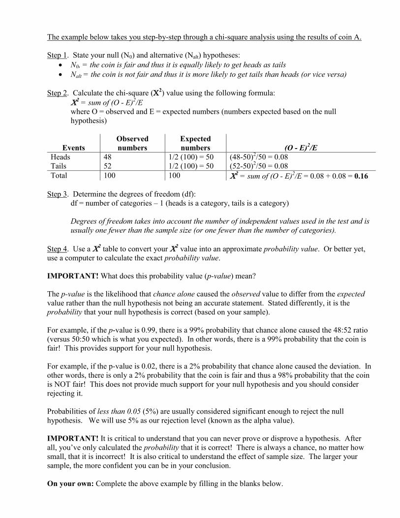
The example below takes you step-by-step through a chi-square analysis using the results of coin A.
Step 1. State your null (N0) and alternative (Nalt) hypotheses:
N0, = the coin is fair and thus it is equally likely to get heads as tails
Nalt = the coin is not fair and thus it is more likely to get tails than heads (or vice versa)
Step 2. Calculate the chi-square (2) value using the following formula:
2 = sum of (O - E)
2/E
where O = observed and E = expected numbers (numbers expected based on the null
hypothesis)
Events
Observed
numbers
Expected
numbers
(O - E)2/E
Heads 48 1/2 (100) = 50 (48-50)2/50 = 0.08
Tails 52 1/2 (100) = 50 (52-50)2/50 = 0.08
Total 100 100 2 = sum of (O - E)
2/E = 0.08 + 0.08 = 0.16
Step 3. Determine the degrees of freedom (df):
df = number of categories – 1 (heads is a category, tails is a category)
Degrees of freedom takes into account the number of independent values used in the test and is
usually one fewer than the sample size (or one fewer than the number of categories).
Step 4. Use a 2 table to convert your 2
value into an approximate probability value. Or better yet,
use a computer to calculate the exact probability value.
IMPORTANT! What does this probability value (p-value) mean?
The p-value is the likelihood that chance alone caused the observed value to differ from the expected
value rather than the null hypothesis not being an accurate statement. Stated differently, it is the
probability that your null hypothesis is correct (based on your sample).
For example, if the p-value is 0.99, there is a 99% probability that chance alone caused the 48:52 ratio
(versus 50:50 which is what you expected). In other words, there is a 99% probability that the coin is
fair! This provides support for your null hypothesis.
For example, if the p-value is 0.02, there is a 2% probability that chance alone caused the deviation. In
other words, there is only a 2% probability that the coin is fair and thus a 98% probability that the coin
is NOT fair! This does not provide much support for your null hypothesis and you should consider
rejecting it.
Probabilities of less than 0.05 (5%) are usually considered significant enough to reject the null
hypothesis. We will use 5% as our rejection level (known as the alpha value).
IMPORTANT! It is critical to understand that you can never prove or disprove a hypothesis. After
all, you’ve only calculated the probability that it is correct! There is always a chance, no matter how
small, that it is incorrect! It is also critical to understand the effect of sample size. The larger your
sample, the more confident you can be in your conclusion.
On your own: Complete the above example by filling in the blanks below.

Restate the null hypothesis.
2 = _______ , df = _______ (copy these values from above)
Based on a chi-square table, the probability (p) of the observed 48:52 heads:tails ratio being
due to chance and sampling error rather than an actual difference from 50:50 is
_________________________________________ %.
Based on the computer calculation, the exact probability is ____________%.
In your own words, what does this particular p-value mean stated in terms of the null
hypothesis?
Based on 5% as the rejection level, do you reject the null hypothesis? ______________
Does this prove that the coin is fair? __________ Why or why not?
On your own: Do a chi-square analysis for each of the other three coins and record the results below.
Observed Expected
Coin H T H T 2 df p(table) p(computer)
A 48 52 50 50 0.16 1 between 50% and 90%
B
C
D
Question: As the observed deviation from expected increases, what happens to the chi-square value?
Question: As the observed deviation from expected increases, what happens to the p-value?
Question: Do the four p-values above agree with your initial rankings?
Question: What is in the chi-square formula that allows it to come to the same conclusion that you did
using your common sense?

Gene Expression and Inheritance in Corn
Goal: To understand how gene expression leads to an observed phenotype and to use chi-square analysis to test a hypothesis.
Part I
Given the following parental genotypes and cross...
Male Female
T/t ; B/b x T/t ; B/b
a) based on the genotype, what is the phenotype of the parents? ___________________
-----------Complete the following four problems (neatly presented) on a separate sheet-----------
b) sketch cells representing both parents (illustrating their chromosomal and allelic makeup)
c) sketch cells representing each genetically-unique gamete produced by both parents
d) using your knowledge of probabilities, predict the phenotypic ratios of their progeny
e) for each progeny phenotype, sketch all unique cells (genotypes) that can produce this
phenotype
Part II
We think that the ear of corn you will be examining includes progeny of the cross shown above. Use a
chi-square analysis to test this hypothesis.
a) State the null hypothesis in terms of the expected phenotypic ratio.
b) Count the number of kernels exhibiting each phenotype.
phenotype observed number total observed _________
Yellow ______
Purple ______
Red ______
c) Perform the chi-square analysis.
phenotype observed expected (O-E)2/E
Yellow _______ _______ _______
Purple _______ _______ _______
Red _______ _______ _______
X2 = sum of (O-E)
2/E = _____________, df = __________
Using a X2
table, the probability that the null hypothesis is correct is __________________ %
Using the computer, the probability that the null hypothesis is correct is _______________ %
Do you reject the null hypothesis? ____________________
What does the p-value mean stated in terms of the null hypothesis?

Pedigree Analysis
Goal: To infer the underlying mechanisms of gene expression and inheritance by examining pedigrees.
The patterns of inheritance recorded in pedigrees can be used to make inferences about the
underlying mechanisms of gene expression and inheritance. Analyzing the results of specific genetic
crosses is more informative in this regard, but performing such crosses is often not possible or
practical--for example, humans or other animals with long generation times.
The objective of this lab is to familiarize you with the methods of analyzing pedigrees in order
to address the following questions regarding the traits under consideration.
Is the gene influencing the trait autosomal or X-linked?
Is the 'mutant' phenotype dominant or recessive?
What are the genotypes of parents and potential offspring?
What is the likelihood of an unborn offspring being affected?
Proceedure
For each of the four genetic diseases described below, address the above questions.
Phenylketonuria (PKU)
Appears in progeny of unaffected parents
Sexes affected equally
Marfan Syndrome
Phenotype appears in every generation
Parent of affected progeny always affected
Duchene muscular dystrophy
More males affected than females
No progeny of an affected male are affected
All of affected male's daughters will have half of their sons affected
Hypophosphatemia (a type of vitamin D-resistant rickets)
Affected males pass the condition to all their female offspring
Affected females pass condition to half their sons and daughters
Additional questions:
1. Will rare, recessive alleles usually be found in heterozygotes or homozygotes? Why?
2. What impact does inbreeding have on the expression of recessive alleles? Why?

Evolutionary Analysis of Genetic Data
Goal: To use genetic data to infer evolutionary relationships among organisms.
We’ve all seen evolutionary trees depicting hypothetical evolutionary relationships among
various groups of taxa. But do you know how those trees were derived? This exercise focuses on
making an evolutionary tree based on genetic data.
Evolution can be defined as descent with modification, and genetic data provide the strongest
supporting evidence of evolution. Genetic data can be used to explore the evolutionary relationships
among individual organisms, populations, species, and all higher taxonomic levels, including
Kingdoms. How are genetic data interpreted in order to draw these conclusions? The following
analogy is useful.
Imagine a class assignment where 10 students write a 10,000-word essay on a particular topic.
The teacher gets back 10 identical essays. What is the chance that all 10 students came up with an
identical essay? The most likely scenario is that someone must have written the original paper and the
others must have copied. Now imagine that one of the papers (John’s) is perfect but the others contain
several errors. David’s paper is identical to John’s with one exception: word #300 is different. Mike’s
paper is identical to John’s except that there are two mistakes, the same one at word #300 and another
at word #1500. Susan’s paper has those two mistakes and another at word #214. This pattern
continues for the remaining students. How would you interpret this? The same logic involved in
interpreting this example is applied when analyzing genetic data. DNA is passed on from one
individual to another (just like the essays), accumulating changes and errors each time it is copied.
The amino acid sequences provided were obtained from a database available through the
internet using the publicly-accessible Entrez search and retrieval system at
http://www.ncbi.nlm.nih.gov/Entrez/. This database contains DNA and amino acid sequences obtained
by researchers from around the world to be shared with the scientific community.
In this lab, you will be using amino acid and DNA sequences to explore the evolutionary
relationships among vertebrates and among whales and their closest living relatives.
Q1 Draw a tree describing the relationships among the essays described above.
Part I: Vertebrate evolution
Using the myoglobin amino acid sequences provided:
1. Determine the number of amino acid positions that differ relative to the first sequence (in italics).
Amino acids that are identical with the first sequence are indicated by a dot. Deletions are indicated by
a dash. Write these values in the table provided.
2. Calculate the percent difference by dividing the number of different amino acid positions by the
total number of positions.
3. Using the scale provided, draw an evolutionary tree based on the percent difference values
calculated above. Draw lightly in pencil because you will need to erase and redraw.

4. You can fine-tune this tree by searching for ‘shared-derived characters’. A shared-derived character
is any character that is shared by a group of individuals but that is unique (derived) relative to all other
individuals. It is likely that these individuals share a common ancestor that had this character.
5. Join the branches of individuals having ‘shared-derived characters’. The more ‘SDC’s a group of
individuals have, the closer you can join the branches relative to the tips of the branches.
6. The last step is to identify the species and interpret your results. When everyone is finished, I will
provide you with a key identifying the species from which each sequence was derived.
Q2 Does this evolutionary tree fit well with what you know about other types of evidence such as the
fossil record and comparative anatomy?
Q3 Do you think that this gene would be useful for determining evolutionary relationships of human
populations? Why or why not?
Part II: The whale’s closest living relative
For over 100 years, scientists have thought that whales may have evolved from an ungulate
ancestor. Morphology and fossil data support this inference. But which living ungulate is most closely
related to whales? Deer, pigs, hippos, or camels? Fossil evidence is not conclusive at the moment, but
genetic data provide a convincing answer to this question.
Alu elements are not the only DNA sequences that can copy and paste themselves randomly in
the genome. SINES and LINES (short and long interspersed elements) are two additional examples of
this unusual type of DNA sequence. The insertion of these DNA sequences is a random event and,
thus, if two individuals have a SINE or LINE at a particular location in their genome, they must have
inherited that DNA sequence from a common ancestor. This DNA insert would be a ‘shared-derived
character’ and can be used to reconstruct evolutionary relationships.
The following table shows the presence or absence of 18 different SINES and LINES in 4
groups of ungulates and two whales. Each number represents a taxa and each letter represents a
particular SINE or LINE insert. ‘x’s indicate taxa that have a particular DNA insert at a particular
location in their genome. These data are from: Nikaido, Rooney, and Okada. 1999. Phylogenetic
relationships among cetartiodactyls based on insertions of short and long interspersed elements:
__________________ are the closest extant relatives of whales. Proceedings of the National Academy
of Sciences, 96:10261.

Taxa SINE or LINE insert
A B C D E F G H I J K L M N O P Q R
20
21 x x x x x x x x x x
22 x x x x x x x x x x x x
23 x x x
24 x x x x x x x x x x x x x
25 x x x x x x x
Identify groups of taxa that share SINE or LINE inserts (shared-derived characters) and place them on
the tree (provided below) in a way that best fits the data. At the appropriate location on the tree,
indicate which taxa share which inserts. Here’s the general procedure: Decide which taxon is most
dissimilar and place it on the longest branch. All other taxa share which character? Indicate that on
the tree. Of the remaining taxa, which is the most dissimilar? Place it on the next longest branch.
Does it have any unique characters? If so, indicate that on the tree. All remaining taxa share which
character(s)? And so on, and so on...
_______________________
_______________________
_______________________
_______________________
_______________________
_______________________
Q4 According to the tree you just constructed, which ungulate is the closest living relative of the
whales?
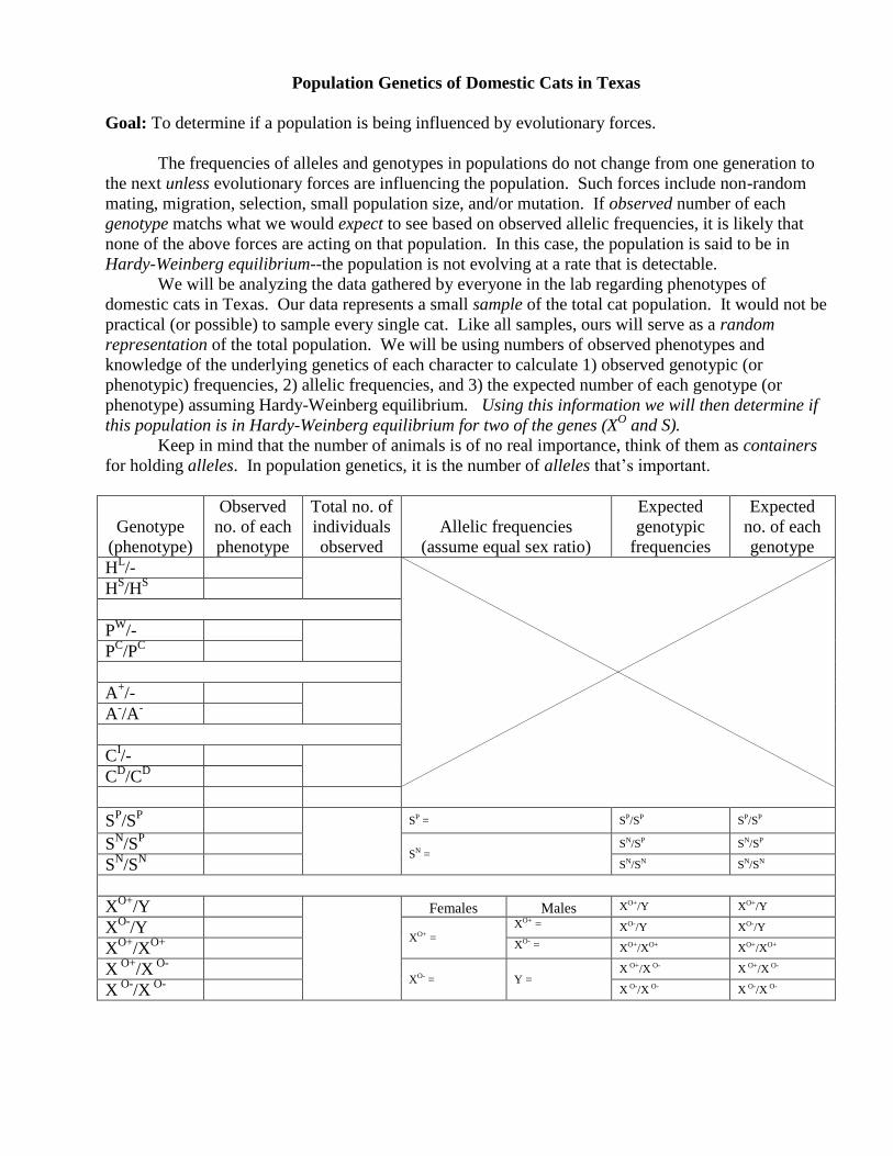
Population Genetics of Domestic Cats in Texas
Goal: To determine if a population is being influenced by evolutionary forces.
The frequencies of alleles and genotypes in populations do not change from one generation to
the next unless evolutionary forces are influencing the population. Such forces include non-random
mating, migration, selection, small population size, and/or mutation. If observed number of each
genotype matchs what we would expect to see based on observed allelic frequencies, it is likely that
none of the above forces are acting on that population. In this case, the population is said to be in
Hardy-Weinberg equilibrium--the population is not evolving at a rate that is detectable.
We will be analyzing the data gathered by everyone in the lab regarding phenotypes of
domestic cats in Texas. Our data represents a small sample of the total cat population. It would not be
practical (or possible) to sample every single cat. Like all samples, ours will serve as a random
representation of the total population. We will be using numbers of observed phenotypes and
knowledge of the underlying genetics of each character to calculate 1) observed genotypic (or
phenotypic) frequencies, 2) allelic frequencies, and 3) the expected number of each genotype (or
phenotype) assuming Hardy-Weinberg equilibrium. Using this information we will then determine if
this population is in Hardy-Weinberg equilibrium for two of the genes (XO and S).
Keep in mind that the number of animals is of no real importance, think of them as containers
for holding alleles. In population genetics, it is the number of alleles that’s important.
Genotype
(phenotype)
Observed
no. of each
phenotype
Total no. of
individuals
observed
Allelic frequencies
(assume equal sex ratio)
Expected
genotypic
frequencies
Expected
no. of each
genotype
HL/-
HS/H
S
PW
/-
PC/P
C
A+/-
A-/A
-
CI/-
CD/C
D
SP/S
P SP = SP/SP SP/SP
SN/S
P
SN = SN/SP SN/SP
SN/S
N SN/SN SN/SN
XO+
/Y Females Males XO+/Y XO+/Y
XO-
/Y XO+ =
XO+ = XO-/Y XO-/Y
XO+
/XO+
XO- = XO+/XO+ XO+/XO+
X O+
/X O-
XO- = Y =
X O+/X O- X O+/X O-
X O-
/X O-
X O-/X O- X O-/X O-

1. State your null hypothesis.
2. Record the observed and expected genotypic frequencies and calculate the 2 value for both genes.
Spot locus
Genotype Observed # Expected # O - E (O - E)2 (O - E)
2 / E
SP/S
P
SP/S
N
SN/S
N
2 =
Orange locus
Genotype Observed # Expected # O - E (O - E)2 (O - E)
2 / E
XO+
/Y
XO-
/Y
XO+
/XO+
X O+
/X O-
X O-
/X O-
2 =
3. Determine the degrees of freedom.
df = [number of categories (genotypes) - 1] - 1 {yes, subtract 1 twice in this case}
4. Convert your 2 value into a probability (p) using a
2 table. p is the probability that your null
hypothesis is correct. Probabilities less than 5% are usually considered significant enough to reject the
null hypothesis. Remember, you can never prove or disprove a hypothesis. After all, you’ve only
calculated the probability that it is correct!
For the piebald spotting locus:
2
= _______ , df = _______
The probability (p) that the null hypothesis is correct is _____________________________
Do you reject the null hypothesis? _____________________
For the orange locus:
2
= _______ , df = _______
The probability (p) that the null hypothesis is correct is _____________________________
Do you reject the null hypothesis? _____________________
Q1 Based on our sample, do you conclude that the local population of cats is in Hardy-Weinberg
equilibrium for the orange (XO) locus? The spot (S) locus?
Q2 In your own words, what do these results mean in terms that anyone could understand?

Population Genetics of Humans
Using the Alu data for the entire lab group, perform a chi-square analysis to test the null hypothesis of
Hardy-Weinberg equilibrium. Keep in mind that the lab group does not represent a true interbreeding
population so don’t be surprised at the results—it could be in equilibrium or it could be out of
equilibrium, depending on the genetic ancestry of the class members.
Genotype Observed Numbers Expected Numbers
Alu+/Alu+
Alu+/Alu-
Alu-/Alu-


