
\STATE ESTIMATION OF UNBALANCED POWER SYSTEMS;
by
Martin,, Wortman
Dissertation submitted to the Faculty of the
Virginia Polytechnic Institute and State University
in partial fulfillment of the requirements for the degree of
DOCTOR OF PHILOSOPHY
APPROVED:
A. G. Phadke
F. C. Brockhurst
in
Electrical Engineering
L. L. Grigs~y~ cK{irman
August, 1982
Blacksburg, Virginia
W. A. Blackwell
C. L. Prather

ACKNOWLEDGMENTS
The author wishes to express his thanks to the many people at
Virginia Tech who have given him encouragement and sound counsel for
the past two and one-half years. Special appreciation is given to
Dr. L. L. Grigsby, Chairman of the author's Advisory Committee, whose
insight and teaching have made the author's graduate study a source of
great satisfaction. Appreciation is also extended to the other members
of the Advisory Committee, including Dr. W. A. Blackwell, Dr. F. C.
Brockhurst, Dr. A. G. Phadke, and Dr. C. L. Prather.
Thanks are given to and for having
provided many valuable suggestions. Appreciation is extended to
, a fellow student and co-worker, for his collaboration
in the modeling and analysis of unbalanced power systems.
Thanks are offered to the participants of the Energy Research
Group; a research assistantship, offered through the ERG, has made
the author's graduate study possible. Thanks are given to
for typing the manuscript.
Finally, thanks are offered to , the author's wife,
whose patience and understanding have been boundless.
ii

TABLE OF CONTENTS
CHAPTER 1. INTRODUCTION •.• 1
1.1 1.2 1.3
Problem Statement State Estimation of Balanced Power Systems • . • • • • Requirements for State Estimation of Unbalanced Power Systems . . . . . . . . . . . . . . . . .
2 3
4
CHAPTER 2. MULTIPORT NETWORK MODELING OF UNBALANCED POWER SYSTfil1S 7
2 .1 General Methodology • • • • • • • • 8 2.2 General Methodology Applied to Power System Segments • 18 2.3 General Methodology Applied to Power Systems • • • 43 2.4 Linear Dependence of Multiport Admittance Matrices
and Normalization of Hultiport Equations . • • • 48
CHAPTER 3. STATE ESTIMATION OF UNBALANCED POWER SYSTEMS • 54
3.1 Extended Method of Weighted Least Squares 55 3.2 Estimator Equations for Unbalanced Power Systems • 59 3.3 Example State Estimates • • • • • • • • • • • • • 70
CHAPTER 4. CONCLUSIONS AND RECOMMENDATIONS FOR FURTHER RESEARCH • 91
4.1 4.2
REFERENCES •
APPENDIX A.
APPENDIX B.
APPENDIX C.
Conclusions . . . . . . . . • . . . . Recommendations for Further Research •
YBUS FROM THE GENERAL METHODOLOGY .
THREE WINDING TRANSFORMER
TAP-CHANGING TRANSFORMER
iii
91 94
102
. 105
• 107
• • 109

CHAPTER 1. INTRODUCTION
The static state of an electric power system is given as a vec-
tor of voltage magnitudes and angles from which all system steady state
voltages can be determined. The static state estimator is a data pro-
cessing algorithm which converts real-time meter readings into an esti-
mate of the static state.
Power systems, due to continually changing load patterns, rarely
achieve a true steady state operating point. It is, however, reason-
able to assume that a power system operates in steady state over some
short time interval. This quasi-steady state behavior suggests that a
static state vector reflects the true system state. Hence, the static
state will be ref erred to as the state and the static state estimator
as the state estimator.
The available literature offers many results concerning the
[1-14] development of state estimators for balanced power systems •
These results address only those systems which can be accurately
represented by a positive sequence network, principally high voltage
bulk transmission networks.
Of increasing interest to the electric utility industry is real-
time monitoring and control of lower voltage distribution networks.
Such networks are, in general, characterized by topological imbalances,
load imbalances, and a varying number of phases per line. Networks
exhibiting these characteristics are ref erred to as unbalanced networks
and cannot be accurately represented by a positive sequence network.
1

2
The results presented here offer a state estimation algorithm
suitable for unbalanced power systems. The algorithm employs a deter-
ministic network model which includes the effects of mutually coupled
conductors, multiple grounding points, unbalanced transformer con-
figurations, and earth return paths. Estimates of the state vector
are in the phase-voltage reference frame.
1.1 Problem Statement
The power system state must be inf erred from real-time meter
readings telemetered from remote points throughout the system to some
central location. These measurements are known to be noise corrupted
and thus do not infer the true system state. The effects of measure-
ment noise can be minimized by the introduction of a state estimator
serving as a noise filter.
The most widely applied method of power system state estimation
is the extended method of weighted least squares. This method requires
that for a system of n state variables, there must be m measurements.
Each measurement is equal to a real function of state variables only,
yielding a set of m equations and n unknowns. The number of measure-
ments m must be greater than the number of state variables n. Further,
there must be n independent equations.
The measured variables are most often real and reactive conductor
power flows, real and reactive loads, and phase voltage magnitudes. The
state variables are most often phase voltage magnitudes and angles.
The power system state estimation problem can be stated as follows:

3
Given m noise corrupted measurements (consist reactive conductor power flows, real and reac phase voltage magnitudes), determine the "bes the system state (n phase voltage magnitudes ; the extended method of weighted least squares
.g of real and
.ve loads, and estimate of
,d angles) by
In a real-time monitoring scenario, the state stimate must be
updated periodically in order to closely approxima : the true system
state. The time interval over which a particular ' ;timate reasonably
approximates the state is determined by the quasi-s ·ady state behavior
of the given system.
1.2 State Estimation of Balanced Power Systems
The following key modeling considerations are :mphasized with
regard to state estimation of balanced power syste1 : •
1) All systems are represented by a positive equence network.
2) All transformers can be represented as eq1 valent IT or T
networks. All transformer banks are bala·. ed.
3) All lines are transposed and can be repre ·nted as equivalent
IT networks.
4) The power system has corrunon datum (ground node.
The above considerations suggest that the sys :ms passive network
(sources and loads excluded) can be modeled by YBU [15] Thus, all
sources and loads are connected at a corrunon earth ·ound node and all
phase voltages are referenced to this node.
For balanced networks, the state vector consi s of all phase
voltage magnitudes and angles. Clearly, load meas ·ements are a
function of YBUS and state variables only. Phase •ltage magnitudes

4
are a function of state variables only. Inasmuch as lines are repre-
sented by II equivalent networks, co~plex conductor power flows can be
obtained from Eq. (1.2.1). Here, S is the complex flow from bus p pq
to bus q as seen at bus p.
s pq
jo -j o V e P (V e P
p p
-jo v e q)(G - jB ) - ·v 2B q pq pq J p c (1.2.1)
Equation (1.2.1) follows directly from the II line selection shown in
Fig. 1. 2 .1.
The simplicity of conductor power flow calculations results from
the absence of mutual coupling between elements of the equivalent II
section of Fig. 1.2.1.
1.3 Requirements for State Estimation of Unbalanced Power Systems
In contrast to state estimation of balanced power systems, the
following modeling considerations are emphasized with regard to state
estimation of unbalanced power systems.
1) Unbalanced systems cannot be represented by a positive sequence
network. All system phases must be explicitly represented.
2) Transformer banks are generally unbalanced. Mutual coupling
between phase windings can exist.
3) Lines and conductors are usually untransposed. Mutual
coupling (inductive and capacitive) can exist. Lines cannot
be represented as equivalent II networks.
4) The earth's surface is a current path of nonzero resistivity.
Thus, the power system can include many earth grounding points.

+
j8 V e P
p
G pq
"B J c
5
B pq
"B J c
Fig. l.2ol. Transmission line equivalent IT.
@
+
j8 V e q
q

6
The above considerations suggest that the system's passive network
(sources and loads excluded) cannot be modeled by YBus· All phase
voltages are referenced to a local neutral or a local ground node;
line-to-line voltages of little practical interest.
Given the state estimation problem statement of Sec. 1.1, a model
for unbalanced networks is required such that noise corrupted measure-
ments are a function of state variables only. The results presented
here offer such a model.
A method to systematically build an admittance matrix for unbal-
anced networks is developed. This admittance matrix exhibits the
mathematical properties of YBUS and is applicable to both balanced
and unbalanced networks.
The network admittance matrix is obtained from subnetwork admit-
tance matrices. The network and subnetwork admittance matrices can be
used to obtain load flow equations suitable for a state estimator.
Chapter 2 presents a general methodology for unbalanced network
modeling. The general methodology is applied to both power subnetworks
(segments) and networks. All admittance matrices are developed in the
phase voltage reference frame.
Chapter 3 contains a development of state estimator equations for
unbalanced power systems. The model of Chapter 2 is incorporated into
the extended method of weighted least squares. The concept of port
suppression is employed so that only nondeterministic measured vari-
ables are included in the estimator equations. The state estimator is
demonstrated via simulation. Example simulations are offered for both
balanced and unbalanced power systems.

CHAPTER 2. MULTIPORT NETWORK MODELING OF UNBALANCED POWER SYSTEMS
The network model offered in the sections to follow is intended to
represent unbalanced power systems operating in steady state. The model
yields a set of complex algebraic equations in variables convenient for
state estimation.
The general methodology for obtaining multiport admittance matrices
of passive networks is presented in Sec. 2.1. The correspondence
between network ports and a given measurement tree is shown. Graph
theoretic principles are used to obtain network multiport equations.
In Sec. 2.2, the general methodology is applied to obtain multiport
equations of power system segments. Multiport equations are developed
such that segment port variables correspond to system state and measured
variables.
In Sec. 2.3, the general methodology is used to obtain multiport
equations of power systems by interconnecting segment multiports. Sys-
tem equations yield port variables that correspond to measured vari-
ables. State variables established by the segment equations are
retained.
Section 2.4 includes a discussion of linear dependence between
port variables. The corresponding rank of multiport admittance
matrices is considered. Normalization of multiport equations via an
appropriate per-unitization scheme is discussed.
7

8
2.1 General Methodology
Development of the general methodology for obtaining multiport
equations of passive networks appeals to linear graph theory. The
following assumptions and definitions are necessary for a graph
theoretic development.
Assumptions and Definitions
1) All networks are represented as directed graphs with spanning
trees and cotrees defined.
t = number of tree branches (twigs)
£ number of cotree branches (links)
2) All network links represent linear passive admittances.
Mutual admittance between links is permitted. Link current/
voltage relationships (primitive equations) can be determined.
3) All network sources belong to the spanning tree (measurement
tree). Sources need not be linear or independent. Dependent
sources must be a function of twig variables.
4) A passive polarity convention is assumed for all branches.
5)
(a) current flow is directed as the branch arrow,
(b) voltage polarity is such that the arrow is directed
towards the negative branch terminal,
(c) positive power indicates dissipation.
A= [A /An], reduced node branch incidence matrix correspond-t1 ~
ing to a given tree. At = tree partition dimensioned t x t;
A2 = cotree partition dimensioned t x £.
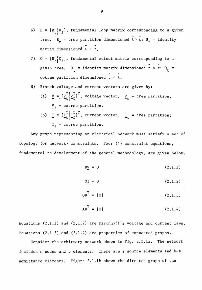
6)
9
B = [B IU 0 ], fundamental loop matrix corresponding to a given ti N
tree. Bt =tree partition dimensioned Q,x t; UQ, =identity
matrix dimensioned Q, x Q,.
7) Q = [Ut!QQ,], fundamental cutset matrix corresponding to a
given tree. ut = identity matrix dimensioned t x t; QQ, =
cotree partition dimensioned t x Q,.
8) Branch voltage and current vectors are given by:
(a)
(b)
v = [vTlvT]T voltage vector. - ~ -tl-Q, '
~Q, = cotree partition. T1 T T
! = [!tl!Q,] , current vector. I
!Q, = cotree partition.
~t = tree partition;
I -t
tree partition;
Any graph representing an electrical network must satisfy a set of
topology (or network) constraints. Four (4) constraint equations,
fundamental to development of the general methodology, are given below.
BV 0 (2.1.1)
QI 0 (2.1.2)
QBT - [O] (2.1.3)
ABT [OJ (2.1.4)
Equations (2.1.1) and (2.1.2) are Kirchhoff's voltage and current laws.
Equations (2.1.3) and (2.1.4) are properties of connected graphs.
Consider the arbitrary network shown in Fig. 2.1.la. The network
includes n nodes and b elements. There are s source elements and b-s
admittance elements. Figure 2.1.lb shows the directed graph of the

Subnetwork of m nodes
and k elements
10
1
2
s
1
2
Subnetwork of n-m nodes
and b-k-S-2 elements
Figo 2ol.la. Arbitrary network of n nodes and b elementso
Subgraph of m nodes
and k branches
1 2
s S+l
: t
1
2
Subgraph of n-m nodes
and b-k-S-2
Fig. 2.1.lb. Directed graph corresponding to the arbitrary network.

11
given network. Darkened branches indicate twigs.
By definition, all source branches belong to the measurement tree
and all admittance branches to the cotree. In general, source branches
are a subset of the twigs. Non-source twigs correspond to no network
elements and do not represent a physical current path. Hence, t-s
non-source twigs are introduced to complete a spanning tree. Note that
the set of all sources can be the null set.
The measurement tree spans all network nodes twig terminal nodes
define unique network node pairs. These node pairs can be considered
ports. Hence, the cotree represents a multiport network.
It is desirable to obtain a set of equations which describe the
steady state behavior of the multiport network in terms of its port
variables. By assumption, the phasor equation describing any admit-
tance branch k is given by
(2.1.5)
where,
number of admittance branches (links)
self-admittance of link k
mutual admittance between links k and i.
It follows from Eq. (2.1.5) that the phaser equations describing
all admittance branches (primitive equations) are given in matrix form
as
(2.1.6)

12
where
Yi t x £ primitive admittance matrix.
From Eqs. (2.1.1) and (2.1.2) it can be shown that
-I -t
-B V t -t
(2.1.8)
(2.1.9)
Thus, the negative of the port currents are a linear combination of
link currents. Link voltages are a linear combination of port voltages.
From Eq. (2.1.3) it can be shown that
-B t
It follows that Eq. (2.1.9) ~an be rewritten as
V = QT V -£ £ -t
Premultiplying Eq. (2.1.6) by the cotree partition of the
fundamental cutset matrix yields
Substituting Eqs. (2.1.8) and (2.1.11) into Eq. (2.1.12) gives
(2 .1.10)
(2.1.11)
(2.1.12)
(2.1.13)
Equation (2.1.13) describes the network steady state behavior in terms
of port variables. For convenience, let the admittance matrix relating
port currents to port voltages be given by

13
(2.1.14)
Thus, the network multiport equations are
-I = y v I -t t -t . (2.1.15)
where Yt is referred to as the multiport admittance matrix. Appendix A
offers a development showing YBUS to be a special case of the multiport
admittance matrix.
The set of all sources is known to be a subset of the twigs for a
given measurement tree. If the set of all sources is not equal to the
null set, then the multiport equations can be rewritten in terms of
source-port variables only via a procedure known as "port sup-
pression". [ 161
where
Let Eq. (2.1.15) be reordered and partitioned such that
!tl
!t2
~tl
~t2
t
sxl
hxl
sxl
hxl
s+h,
[ ~~==] -t2
[ ;===-f-;===] [~tl] t21 I t22 -t2
(2.1.16)
vector of source-port currents
vector of currents corresponding to ports without sources
vector of source-port voltages
vector of voltages corresponding to ports without sources
number of ports
If the terminal nodes of a non-source twig are incident to only
branches belonging to the multiport network, then the non-source port

14
current is zero. Thus, for the network of Fig. 2.1.1
.!t2 = 0 (2.1.17)
It follows that Eq. (2.1.17) can be separated into the two
matrix equations
-I -tl
0 y v + y v t21 -tl t22 -t2
where,
ytll = sxs admittance matrix
ytl2 sxh admittance matrix
yt21 hxs admittance matrix
yt22 = hxh admittance matrix
Solving Eq. (2.1.19) for non-source port voltages yields
v -t2
Substituting Eq. (2.1.20) into Eq. (2.1.18) gives
(2.1.18)
(2.1.19)
(2.1.20)
(2.1.21)
The multiport equations of Eq. (2.1.21) now describe the steady
state behavior of the network in terms of source variables only. With
non-source ports suppressed, the order of the multiport admittance
matrix is s. In practical situations, s can be much less than t.

15
Given the source voltages V 1 , non-source port voltages and net--t
work link voltages can be recovered from Eqs. (2.1.20) and (2.1.11)
respectively.
Simple Example
Consider the simple system shown in Fig. 2.l.2a. The admittance
network (sources excluded) consists of six (6) admittance elements,
each with a self admittance of 1.0~. Two (2) of the elements are
mutually coupled with a mutual admittance of 0.5~.
Figure 2.l.2b shows the network graph with a measurement tree,
defining ports, introduced. Darkened branches indicate twigs.
Primitive equations describing the steady state behavior of the
admittance network are given by
1£1 1.0 -0.5 0 0 0 0 vi1
1£2 -0.5 1.0 0 0 0 0 vi2
1£3 0 0 1.0 0 0 0 v£3 (2.1.22)
1£4 0 0 0 1.0 0 0 v£4
1£5 0 0 0 0 1.0 0 vis
1£6 0 0 0 0 0 1.0 v£6
The fundamental cutset matrix corresponding to the specified
measurement tree is given by

16
1.0v l.Ov
I O.Sv
1.0v I t ! 1.0 v
I
l.Ov l.Ov
Fig. 2.l.2a. Simple network.
Fig. 2.l.2b. Network graph with measurement tree.

17
tl t2 t3 t4 ts Q,l Q, 2 Q, 3 Q, 4 Q, s Q, 6
tl 1 0 0 0 0 -1 0 0 0 0 0
t2 0 1 0 0 0 1 1 0 -1 0 0
Q t3 0 0 1 0 0 0 0 0 1 1 0 (2.1.23)
t4 0 0 0 1 0 -1 0 1 1 0 1
ts 0 0 0 0 1 0 0 0 -1 0 -1
The network multiport admittance matrix, y t' is now given by
1.0 -0.5 0 1. 0 0
-0.S 2.0 -1. 0 -1.5 1.0
y QQ, YQ, t QT
Q, 0 -1.0 2.0 1. 0 -1.0 (2.1.24)
1.0 -1.5 1.0 4.0 -2.0
0 1.0 -1.0 -2.0 2.0
Thus, the network steady state behavior expressed in terms of port
variables is given by
I 1.0 tl
-0.S 0 1.0 0 v tl
I -0.S t2
2.0 -1.0 -1. s 1.0 v t2
(2.1.25) I 0
t3 -1.0 2.0 1. 0 -1. 0 v
t3
I 1.0 -1.5 1. 0 4.0 -2.0 v t4 t4
I ts
0 0 1.0 -2.0 2.0 v ts

18
Equation (2.1.25) is partitioned so as to indicate source ports and
non-source ports.
The steady state behavior of the network can be described in
terms of source port variables only. From Eq. (2.1.21) it follows that
1.0 -0.5 0 1.0 0
-0.5 2.0 -1.0 -1.5 1.0
2.0 1.0 -1.0 -1 0 -1.0 v tl
1.0 4.0 -2.0 1.0 -1.5 v
-1.0 -2.0 2.0 0 1.0 t2
(2.1.26)
Thus, the network multiport equations, after port suppression, are
given by
I 0.500 -0.250 v tl tl
(2.1.27) I t2
-0.250 1.208 v t2
2.2 General Methodology Applied to Power System Segments
Application of the general methodology to the multiport modeling
of power system segments requires that the power system be represented
as a directed graph. To this end, power systems will be defined as
sources and loads connected by an admittance network. All system
loads are specified as constant complex power sources.

19
The admittance network connecting sources and loads consists of
admittance elements modeling power system components which can be
inductively and/or capacitively coupled.
When the admittance network is represented as a directed graph, a
segment is defined as follows:
A set of connected and/or mutually coupled branches. All segments must include at least one branch. Each network branches belong to one and only one segment.
The admittance network of a power system consists of three prin-
cipal segment types: (1) conductor segments, (2) transformer segments,
and (3) auxiliary device segments. Multiport equations for the three
segment types will be developed.
Conductor Segments
Consider the conductor ~egment shown in Fig. 2.2.1. Here, n-1
conductors are positioned above and parallel to the earth's surface.
The earth's surface is considered a homogeneous medium of nonzero
resistivity.
A number of techniques for developing .lumped parameter models of
parallel conductors with earth return exist.[ll,lS] For the purposes
of this development, Carson's equations are employed.[l 9 ] Much litera-
ture has been devoted to Carson's equations.[ 20, 2l] Hence, only the
applicable results are considered.
Carson's equations allow for inductive coupling between all seg-
ment conductors where the earth's surface is modeled as an equivalent
conductor. Carson's results indicate that the steady state behavior
of the segment is given by

Q G)
Q
20
1
2
3
k
n-1
Earth's Surface
/7777777777777//7///7/77
Fig. 2.2.1. Conductor segment of n-1 conductors above and parallel to the earth's surface.

where,
~p L
21
~p nxl vector of voltages across conductors L
~p nxl vector of currents through conductors L
(2.2.1)
Zp nxn impedance matrix (on-diagonal elements are self L impedances, off diagonal elements are mutual reactances).
The directed graph corresponding to the conductor segment
inductive effects and Eq. (2.2.1) is shown in Fig. 2.2.2.
Each conductor segment includes a single earth equivalent (ground)
conductor. A segment of n conductors has 2n nodes, n nodes at each end
of the segment. The terminal nodes of the ground conductor are referred
to as ground nodes. Terminal nodes of neutral conductors are neutral
nodes and terminal nodes of phase conductors are phase nodes.
Equation (2.2.1) is often formulated in a manner such that the
conductor currents I sum to zero.[ 20] This added constraint suggests -PL
that current through the ground conductor is a linear combination of
all other segment conductor currents. When this constraint is enforced,
the ground conductor of Fig. 2.2.1 must be suppressed. With the ground
conductor suppressed, the ground conductor branch of Fig. 2.2.2 is
eliminated while its terminal nodes (ground nodes) remain a part of
the segment graph.
The n nodes at a given end of a segment are said to "correspond",
indicating that they are terminal nodes at the same end of the seg-
ment. Thus, a ground node can have no more than n-1 corresponding
phase nodes. Similarly, a neutral node can have no more than n-2

Q Q G)
G
22
1
2
3
k
n-1
Equivalent earth conductor branch
Fig, 2.2.2. Directed graph of conductor segment inductive effects.

23
corresponding phase nodes.
In addition to inductive coupling effects, long conductor segments
can exhibit capacitive coupling between conductors. Modeling of capac-
itive coupling most often relies on the method of images.[ 22 ] Much
literature has been devoted to the modeling of power conductor capaci-
. l" b h h d of . [20,21,23] tive coup ing y t e met o images. Only the applicable
results are considered here. Although not exact, experience has shown
this method is a realistic approximation.
At the relatively low frequencies characteristic of power systems,
conductors are assumed to have linear charge density. The earth's sur-
face is considered a perfectly conducting ground plane. Under these
assumptions, it is possible to express voltages between conductors and
the earth's surface as a function of conductor charge by
v Pg (2.2.2)
where,
V (n-l)xl conductor to earth voltage vector
g = (n-l)xl charge vector
P (n-l)x(n-1) potential matrix
The potential matrix P is known to be nonsingular; thus,
Eq. (2.2.2) can be rewritten as
(?..2.3)
The elements of P-l are called Maxwell's coefficients.[ 23 , 24 ]
The capacitive coupling between any two conductors and between any
24
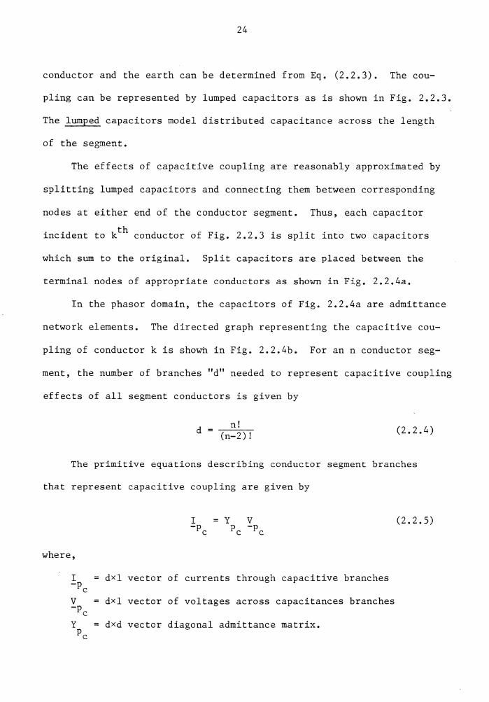
conductor and the earth can be determined from Eq. (2.2.3). The cou-
pling can be represented by lumped capacitors as is shown in Fig. 2.2.3.
The lumped capacitors model distributed capacitance across the length
of the segment.
The effects of capacitive coupling are reasonably approximated by
splitting lumped capacitors and connecting them between corresponding
nodes at either end of the conductor segment. Thus, each capacitor
incident to kth conductor of Fig. 2.2.3 is split into two capacitors
which sum to the original. Split capacitors are placed between the
terminal nodes of appropriate conductors as shown in Fig. 2.2.4a.
In the phasor domain, the capacitors of Fig. 2.2.4a are admittance
network elements. The directed graph representing the capacitive cou-
pling of conductor k is shown in Fig. 2.2.4b. For an n conductor seg-
ment, the number of branches "d" needed to represent capacitive coupling
effects of all segment conductors is given by
d n! (2.2.4) (n-2) !
The primitive equations describing conductor segment branches
that represent capacitive coupling are given by
where,
I dxl vector -pc v = dxl vector -pc y dxd vector
pc
y v pc -pc
of currents through capacitive branches
of voltages across capacitances branches
diagonal admittance matrix.
(2.2.5)

25
1 3
k
Fig. 2.2.3. Lumped capacitance between conductors and earth.

Fig. /..2.4a.
Fig. 2.2.4b.
26
G
earth grounding
th Lumped capacitance of k conductor split between corresponding segment nodes.
0 0
G)
Direct graph representing capacitive coupling of the kth conductor.

27
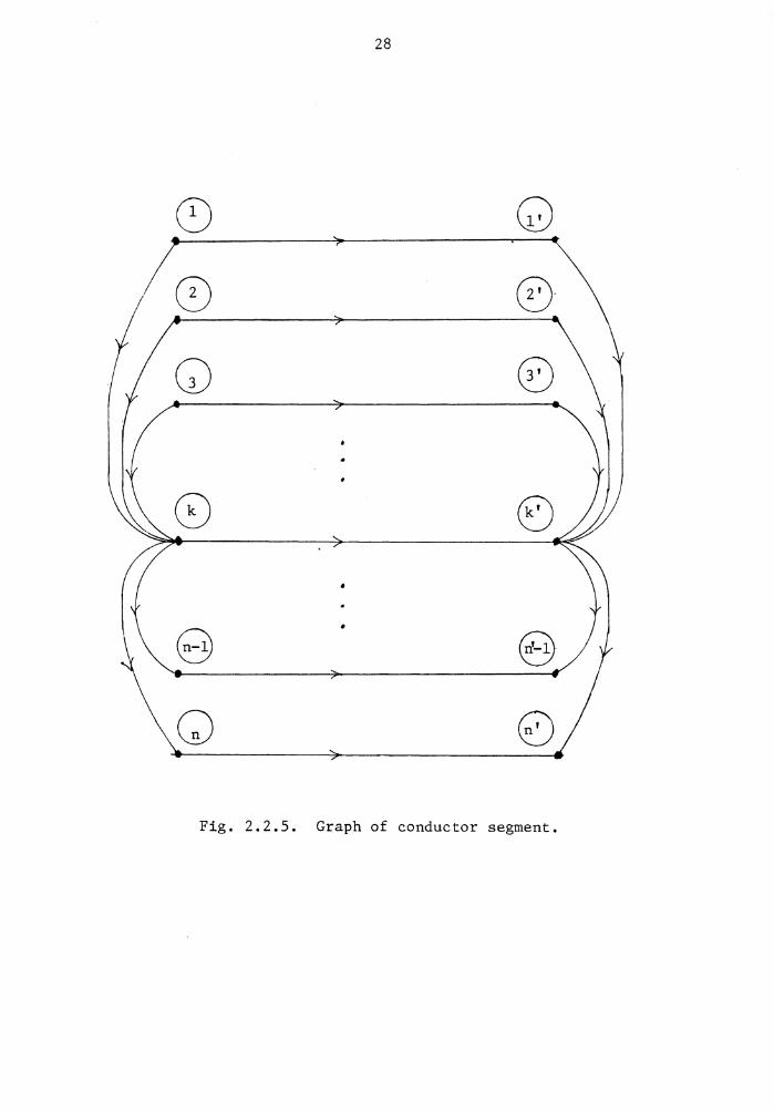
The complete graph of the conductor segment is given by the union
of graphs representing inductive effects and capacitive effects. A
graph representing the segment of Fig. 2.2.1 is shown in Fig. 2.2.5. th (For convenience, only capacitive branches corresponding to the k
conductor are shown.)
The steady state behavior of the conductor segment is given by
where,
I -p
v -p
y p
IT ]T p ' c
I -p y v
p -p
(n+d)xl vector of branch currents
= [~~ ~~ ]T, (n+d)xl vector of branch voltages L C
, (n+d)x(n+d) admittance matrix.
(2.2.6)
Equation (2.2.6) describes a general segment of overhead con-
ductors. It is recognized that the segment can include any number
of multiphase lines. If neutral phases are present, each neutral
will have a set of corresponding power phases. It is noted that
equations describing segments of underground cable can be obtained[ 2S]
and an analogous graph constructe<l.
The conductor segment of Fig. 2.2.1 can be considered a multiport
network. The general methodology is to be applied such that port vari-
ables are in a suitable voltage reference frame for state estimation.
It follows that a measurement tree must include twigs defining
ports in the phase-voltage reference frame. Thus, the following rule
28
0-
Q 0
Fig. 2.2.5. Graph of conductor segment.

29
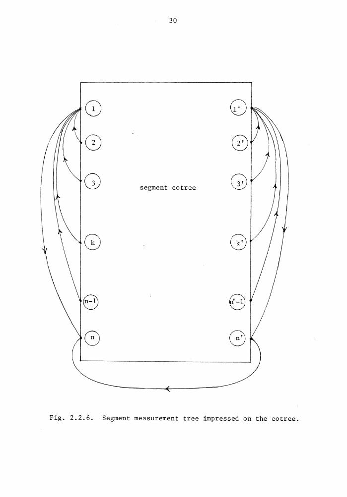
for introducing conductor segment measurement trees is given.
A twig is introduced between ground nodes. Twigs are introduced between ground nodes and their corresponding neutral nodes. Twigs are introduced between neutral nodes and all of their correspond-ing phase nodes. If no neutral conductor is present, twigs are introduced between ground nodes and all of their corresponding phase nodes. Ground and neutral nodes can be coincident.
st If the 1 conductor is neutral, the measurement tree for the con-
ductor segment of Fig. 2.2.1 is shown in Fig. 2.2.6. With the intro-
duction of a measurement tree, the graph of Fig. 2.2.5 becomes the
segment cotree.
Let the segment port voltages and port currents be written as
V (2n-l) vector of segment port voltages -m
I = (2n-l) vector of segment port currents. -m
From Eqs. (2.1.8) and (2.1.11) it is known that
where,
-I -m
v -p QT V
p -m
QP = cotree partition of the fundamental cutset matrix corresponding to the given measurement tree.
(2.2.7)
(2.2.8)
Premultiplying Eq. (2.2.6) by Q and substituting Eqs. (2.2.7) and p
(2.2.8) yields
-I = Q Y QT V -m p p p -m (2.2.9)
Equation (2.2.9) give the segment multiport equations and are rewritten
as
-I = Y V -m m -m (2.2.10)
30
segment cotree
Fig. 2.2.6. Segment measurement tree impressed on the cotree.

31
where
T Ym = Qp Yp Qp, the segment multiport admittance matrix.
Complex power flow in the phase conductors can be determined from
the segment multiport equations. Let complex power flowing in the kth
conductor be denoted as Tkk' + jUkk' indicating the flow from node k to
node k' as would be measured at node k.
Cl 1 h 1 . . d . h kt h d ear y, t e comp ex power inJecte into t e con uctor at
th node k is the negative of the k port complex power. Thus complex
conductor flow is given by
where,
V voltage across phase port k mk
I current through phase port k. mk
(2.2.11)
Equation (2.2.11) can be rewritten in terms of multiport admittance
matrix elements and port voltages
where
y ~i
2n-l v l
mk i=l * v m.
l
(2.2.12)
element of the multiport admittance matrix in the row corresponding to port k and the ith column.
Hence, line flows can be given as a function of port variables only.

32
Equation (2.2.10) suggests that the segment can be graphically
represented by the measurement tree alone. That is, the conductor
segment is represented as the set of mutually coupled branches shown
in Fig. 2.2.7. This graph is called the modified segment. Primitive
equations describing the modified segment are given by
I = Y V -m m .-m
(2.2.13)
Transformer Segments
Consider the circuit of Fig. 2.2.Sa representing a nonideal two-
winding transformer. Winding losses are reflected to the primary side;
core losses are not considered.
Transformer banks are often modeled as a set of two-winding trans-
formers appropriately interconnected. Here, multiport transformer
segment models will consider only segments with two-winding trans-
formers. Multiports for segments of three-winding and tap-changing
transformers are given in Appendices B and C respectively.
The transformer of Fig. 2.2.Sa is described by the following two
port equations
(2.2.14)
where,
transformer loss admittance
a = reciprocal of the turns ratio.

33
Q G
Fig. 2.2.7. Modified segment primitive.

34
a:l )
Fig. 2.2.Sa. Two winding transformer.
1
2
Fig. 2.2.Sb. Transformer primitive branches.

35
Equation (2.2.14) suggest that the transformer can be represented by
the two mutually coupled branches shown in Fig. 2.2.Sb. These branches
are called transformer primitive branches. The primitive equations for
these branches are given by
(2.2.15)
With transformers represented by primitive branches, transformer
segments are defined as follows:
A set of connected transformer primitive branches and admit-tance branches. Admittance branches represent grounding admittances. The segment has only one ground node.
Primitive equations for a transformer segment are given by
I y 0 v -p T PT -pT
--------- (2.2.16) I 0 y v -p g pg -p g
where,
I vector of currents through transformer primitive branches -pT
I vector of currents through grounding admittance branches -p g
V vector of voltages across transformer primitive branches -p T
V vector of voltages across grounding admittance branches -p g
Y block diagonal matrix of transformer admittances PT

36
Y diagonal admittance matrix. Pg
For convenience, let Eq. (2.2.16) be rewritten as
I = Y V -p p -p (2.2.17)
Transformer segments can be considered multiports; hence, it is
necessary to introduce a measurement tree such that defined ports are
in the phase voltage reference frame.
Terminal nodes of transformer primitive branches define segment
primary and secondary nodes (as with any transformer bank), Phase
nodes of the primary correspond; phase nodes of the secondary
correspond. If a neutral node (nodes) is present, it (they)
can correspond to: (1) primary nodes only, (2) secondary nodes only,
(3) both primary and secondary nodes. Neutral nodes can be coincident
with the ground node (i.e. solidly grounded neutrals).
The transformer segment measurement tree is defined as follows:
Twigs are introduced between the ground node and all neutral nodes not coincident with the ground. Twigs are introduced between all neutral nodes and their corresponding phase nodes. For phase nodes with no corresponding neutral, twigs are introduced between phase and ground.
The segment graph for a delta-wye (secondary grounded through an
admittance) transformer bank is shown in Fig. 2.2.9a. The segment
measurement tree is shown in Fig. 2.2.9b.
Transformer primitive and grounding admittance branches now com-
prise the segment cotree. With a segment measurement tree introduced,
it is desirable to obtain multiport equations describing the steady
state behavior of the segment in terms of port variables.

37
. [a primary phase nodes :
secondary phase nodes
'----- n secondary phase nodes
/ _l_ g segment ground nodes
Fig. 2.2.9a. Delta-wye transformer bank segment with secondary grounding admittance.
a
g
Fig. 2.2.9b. Delta-wye transformer bank segment with measurement tree.

38
For an n node transformer segment, let the segment port voltages,
currents, and fundamental cutset matrix cotree partition be written as
v -m I -m
(n-l)xl vector of segment port voltages
(n-l)xl vector of segment port currents
cotree partition of the fundamental cutset matrix corres-ponding to a given segment measurement tree.
The segment cotree is described by Eq. (2.2.17). When the general
methodology is employed, the segment multiport equations are given by
-I -m (2.2.18)
For convenience, the segment multiport equations can be rewritten as
-I -m
where
y v m -m (2.2.19)
T Y = Q Y Qp' (n-l)x(n-1) segment multiport admittance matrix. m p p
Equation (2.2.19) suggests that the transformer segment can be
graphically represented by its measurement tree alone. Thus, the
segment is comprised of n-1 mutually coupled branches. These branches
are called the modified primitive branches and collectively are called
the modified segment. Equations describing the steady state behavior
of the modified segment are given by
I -m y v
m -m (2.2.20)
The modified segment for the delta-wye transformer bank of Fig. 2.2.9a
is shown in Fig. 2.2.10.

39
a'
b b'
I c'
n
g
Fig. 2.2.10. Modified segment primitive for Delta-wye transformer bank.

40
Transformer segments, when modified, are described in the phase
voltage reference frame and, thus, in terms of state variables.
Auxiliary Device Segments
Power systems often include auxiliary devices such as capacitor
banks. It is assumed that any auxiliary device can be represented as
a set of lumped admittances. When represented as a directed graph,
auxiliary device segments are defined as follows:
A set of connected admittance branches. Terminal nodes of the segment branches define phase nodes and no more than one neutral node. All segment nodes (phase and neutral) corres-pond to a single ground node. Ground and neutral nodes can be coincident.
The segment branches are assumed to be lumped admittances and
the steady state behavior of the segment is given by
I y v (2.2.21) -p p -p
where,
I vector of segment branch currents -p
v vector of segment branch voltages -p y primitive admittance matrix. p
Auxiliary device segments are considered multiport networks;
thus, a segment measurement tree defining ports can be introduced.
The segment measurement tree is defined as follows.
A twig is introduced between the ground and neutral nodes. Twigs are introduced between all phase nodes and the neutral. If the ground and neutral are coincident or if no neutral is present, twigs are introduced between all phase nodes and ground.

41
With a segment measurement tree introduced, it is desirable to
describe the segment steady state behavior in terms of port variables.
The segment cotree is comprised of primitive admittance branches. Let
the port voltages currents, and cotree partition of the fundamental cut-
set matrix (corresponding to a specified measurement tree) be given by
V vector of port voltages -m I vector of port currents -m Qp cotree partition of the segment fundamental cutset matrix
When the general methodology is employed, multiport equations for
the segment are given by
-I -m (2.2.22)
A wye-connected capacitor bank with a grounding admittance ~s
shown in Fig. 2.2.lla. The segment graph and measurement tree are
shown in Fig. 2.2.llb.
Equation (2.2.22) suggests that an auxiliary device segment can
be represented graphically by the segment measurement tree alone.
Hence, the segment is represented as a set of mutually coupled
branches called modified primitive branches. Collectively, the
modified primitive branches are the modified segment. Equations
describing the modified segment are given by
where,
I -m y v
m -m
Y = Qp Y QT segment multiport admittance matrix. m p p'
(2.2.23)

42
c g
Fig. 2.2.lla. Wye-connected capacitor bank with grounding admittance.
a capacitor bank
segment b
Fig. 2.2.llb. Capacitor bank segment graph and measurement tree.

43
The modified segment for the wye-connected capacitor bank of
Fig. 2.2.lla is shown in Fig, 2.2.12.
2.3 General Methodology Applied to Power Systems
Having applied the general methodology to all power system seg-
ments, the power system admittance network (sources and loads
excluded) is represented as the union of all modified segments. The
union of all modified segments is called the modified primitive
network. Equations describing the steady state behavior of the
modified primitive network for a system of q segments is given by
~~ y 0 ... 0 . .. 0 v
ml -ml
I 0 ~ 0 0 v -m2 m2 -m2
(2.3.1)
I 0 0 ..• y 0 v -m. m. -m. 1 1 1
L~ 0 0 0 •.. y v m -m q q
For convenience, Eq. (2.3.1) can be rewritten as
where,
I -m
v -m y
m
I y v -m m -m (2.3.2)
vector of modified primitive network currents
vector of modified primitive network voltages
block diagonal admittance matrix. The diagonal blocks are segment multiport admittance matrices.

44
a b
n
c
Fig. 2.2.12. Modified segment of wye-connected capacitor bank.
45
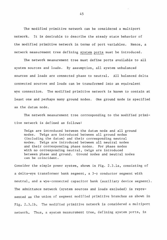
The modified primitive network can be considered a multiport
network. It is desirable to describe the steady state behavior of
the modified primitive network in terms of port variables, Hence, a
network measurement tree defining system ports must be introduced.
The network measurement tree must define ports available to all
system sources and loads. By assumption, all system unbalanced
sources and loads are connected phase to neutral. All balanced delta
connected sources and loads can be transformed into an equivalent
wye connection. The modified primitive network is known to contain at
least one and perhaps many ground nodes. One ground node is specified
as the datum node.
The network measurement tree corresponding to the modified primi-
tive network is defined as follows:
Twigs are introduced between the datum node and all ground nodes. Twigs are introduced between all ground nodes (including the datum) and their corresponding neutral nodes. Twigs are introduced between all neutral nodes and their corresponding phase nodes. For phase nodes with no corresponding neutral, twigs are introduced between phase and ground. Ground nodes and neutral nodes can be coincident.
Consider the simple power system, shown in Fig. 2.3.la, consisting of
a delta-wye transformer bank segment, a 3-¢ conductor segment with
neutral, and a wye-connected capacitor bank (auxiliary device segment).
The admittance network (system sources and loads excluded) is repre-
sented as the union of segment modified primitive branches as shown in
Fig. 2.3.lb. The modified primitive network is considered a multiport
network. Thus, a system measurement tree, defining system ports, is

3<P source t:,-Y Transf orme Segment
Fig. 2.3.la.
46
~ductor Segment )¢ load capacitor
Simple power system.
Transformer segment Conductor segment Auxiliary Device
Segment
~ \ '/~,-..
\\ \,<(\~.' ~ \. i • .+- '~ I / . 'V
\-4 \' ./'." \ '' ' \ !; .... lj \ :~ ' I "!//
Fig. 2.3.lb. Modified primitive network (sources and loads excluded).
Fig. 2.3.lc. I1odified ririmitive network with c-Jeasurement tree. Twigs are darkened branches.

47
introduced. The modified primitive network with the system measurement
tree is shown in Fig. 2.3.lc.
With a system measurement tree introduced in the fashion des-
cribed above, the following port definitions are offered: (1) a twig
incident only to ground nodes defines a ground port, (2) a twig inci-
dent to neutral and ground nodes defines a neutral port, and (3) a
twig incident to any phase node defines a phase port. State variables
are phase port voltage magnitudes and angles. All system sources and
loads are connected at available phase ports.
It follows that the general methodology can be used to obtain
multiport equations for the modified primitive network. For a system
of n nodes, let the system port voltages and currents be given by
V (n-1) vector of sy~tem port voltages -t
!t (n-1) vector of system port currents.
By Eqs. (2.1.8) and (2.1.11) it can be shown that
where,
-I -t
v -m QT V
m -t
(2.3.3)
(2.3.4)
cotree partition of the fundamental cutset matrix corres-ponding to the system measurement tree and the modified primitive network.
Premultiplying Eq. (2.3.2) by the cotree partition of the cutset
matrix yields
(2.3.5)

48
Substituting Eqs. (2.3.3) and (2.3.4) into Eq. (2.2.5) gives
(2.3.6)
Equation (2.3.6) gives the power system multiport equations and can
be rewritten as
-I -t (2.3.7)
where,
T Yt = ~ Ym Qm, (n-l)x(n-1) system multiport admittance matrix.
Hence, Eq. (2.3.6) describes the steady state behavior of a power
system in terms of its port variables.
2.4 Linear Dependence of Multiport Admittance Matrices and Normalization of Multiport Equations
An important consideration with regard to multiport equations is
linear dependence among equations. Linear dependence among equations
obtained by the general methodology is reflected in the rank of the
resulting multiport admittance matrix.
When the general methodology is applied to segments, the
resulting segment multiport admittance matrices are often of non-
zero nullity. Both segment topology and the nature of segment primi-
tive equations can contribute to nullity.
Topological Dependence
Consider first, nullity resulting from segment topology. It can
be shown that the number of independent multiport equations is related

49
to the number of independent segment cutsets.[ 261 Thus, the rank of
the multiport admittance matrix is less than or equal to the rank of
the segment graph. Or,
r < r sm sg (2.4.1)
where,
r rank of the segment multiport admittance matrix sm
r rank of the segment graph. sg
A component of a graph is defined as a connected subgraph con-
taining the maximal number of branches. [ 26 ] It can be shown that for
a segment of n nodes,
where,
r . sg n - c sg
c the number of segment graph components. sg
It follows that
r 2 n - c sm sg
(2.4.2)
(2.4.3)
The nullity, h of a segment multiport admittance matrix is given by sm'
h sm (n-1) - r sm
From Eqs. (2.4.4) and (2.4.3) it can be shown that
h > c - 1 sm sg
(2.4.4)
(2.4.5)

so
Conductor segments can have negligible capacitive coupling
effects. Graphs for such segments include more than one component.
Thus, Eq. (2.4.5) can be used to establish nullity lower bounds for
the resulting multiport admittance matrices.
Dependence ~ Primitive Equations
Linear dependence among primitive (modified primitive) equations
can introduce nullity into multiport admittance matrices. When the
general methodology is employed, the network multiport admittance
matrix is given by Eq. (2.1.14), shown again here.
Let the following matrix ranks be given.
The
r = rank of the multiport admittance matrix Yt yt
r Yi
rank of the primitive admittance matrix Y2
rQ £
rank of the cutset matrix partition Q2
rank rQ can be determined as in Eq. (2.4.2). £ A A
(2.4.6)
For a network of t+l nodes and £ branches, linear dependence among
the primitive equations implies that
But from Sylvester's inequality, it is known that[ 2l]
r < min yt
(r , rQ ). Yi £
(2.4.7)
51
Hence, for rQ Q,
< r < Q, , it is possible to lower bound the nullity Yi
of the multiport admittance matrix.
It is noted here that linear dependence among transformer primi-
tive equations is found in Eq. (2.2.15). Thus, transformer segment
multiport admittance matrices have nonzero nullity.
Normalization of Multiport Equations
Nominal phase voltage magnitudes can vary greatly throughout a
given power system. For this reason, power system equations are most
often normalized such that phase voltage magnitudes are nominally near
unity.
A meaningful normalization scheme for unbalanced power systems
requires that all state estimator equations be in per-unit. Hence,
all segment primitive equations are normalized prior to application
of the general methodology.
The following normalization scheme is used to obtain per-unit
segment primitive equations.
1) A system power base, SB (KVA), is selected. All system
loads are normalized by SB.
2) A base voltage VBC. (KV) is selected for the ith conductor 1
segment. Conductor segment base admittance is given by 2
YBC. = SB/VBC.. Segment base current is given by IBC. = 1 1 1
SB/VBC.. All segment primitive admittances are normalized 1
by y . BC.
1
All segment port voltages are normalized by VBC .. 1
All segment port currents are normalized by IBC . i

52
3) A primary base voltage VBTP. (KV) and a secondary base voltage 1
(KV) . 1 d f h .th f h
4)
5)
VBTS. is se ecte or t e 1 trans ormer segment. Te 1
base turns ratio for segment transformers is given by aBT. = 1
VBTP./VBTS .. Segment primary base current is given by 1 1
Segment secondary base current is given by
Transformer segment base admittance is
2 given by YBT. = SB/VBTP.
1 1
All segment turns ratios are
normalized by aBT .. All segment transformer loss admittances 1
are normalized by YBT .. 1
All primary port voltages are nor-
malized by VBTP .. 1
All secondary port voltages are normalized
by VBTS .. 1
All primary port currents are normalized by IBTP .. 1
All secondary port currents are normalized by IBTS .. 1
A base voltage VBA. (KV) 1
device segment. Segment
. 1 d f h .th ·1· is se ecte or t e 1 auxi iary
2 SB/VBA.
1
base admittance is given by YBA. = 1
Segment base current is given by IBA. = SB/VBA. · 1 1
All segment primitive admittances are normalized by YBA ..
All segment port voltages are normalized by VBA .. 1
ment port currents are normalized by IBA .. 1
1
All seg-
All adjacent segment ports must have the same base voltage.
With all segment primitive equations normalized, the general
methodology yields per-unit multiport equations. Segment port vari-
ables are de-normalized when multiplied by their corresponding base
values.
By definition,system phase and neutral ports correspond directly
to segment phase and neutral ports. Thus, system phase and neutral

53
port variables are de-normalized when multiplied by corresponding
segment port base values,
System ground ports are defined by twigs connected between the
datum and ground nodes of the modified primitive network, Therefore,
system ground ports, in general, can connect segments that are normal-
ized on different base voltages. It follows that ground port base
voltages are unknown. Note, however, that system ground port variables
are of little practical interest. In the event that ground port
voltages are needed, they can be recovered using real units. The
ground voltages of practical are segment ground port voltages.

CHAPTER 3. STATE ESTIMATION OF UNBALANCED POWER SYSTEMS
State estimation of unbalanced power system, as developed in the
sections that follow, appeals to the extended method of weighted least
squares. Least squares estimators are widely accepted within the
electric utility industry; hence, no attempt to examine the estimator's
quality is made.
State estimator equations, to be developed, are a natural result
of the multiport models offered in Chapter 2. Thus, the results
offered in this chapter are intended to demonstrate that unbalanced
power systems can be modeled such that accepted power system state
estimation techniques can be employed.
The extended method of weighted least squares is developed in
Sec. 3.1. The method is presented as a minimum norm estimator. No
statistics are associated with the estimator or model.
Unbalanced power system estimator equations are formulated in
Sec. 3.2. Rules for identifying state variables are given. Port
suppression is employed to obtain multiport equations in terms of
state voltages only. Equations for the estimator model are obtained
from the suppressed multiport equations. Equations yielding entries
of the Jacobian matrix are presented.
The extended method of weighted least squares of Sec. 3.1, along
with the estimator equations of Sec. 3.2, are demonstrated by way of
example in Sec. 3.3.
Example 1 seeks to demonstrate the estimator equations and model-
ing technique for a simple balanced power system. Inasmuch as balanced
54

55
power systems represent a special case of unbalanced multiport
networks, Example 1 verifies the estimator on a system with a well known
solution.
Example 2 demonstrates the estimator equations and model-
ing technique for an unbalanced power system. Example 2 considers a
system containing both load and topological imbalances.
3.1 Extended Method of Weighted Least Squares
Power system state estimation requires that a set of measured
variables be functionally related to the system state. When the mea-
sured variables are noise corrupted, this relationship can be written
as
z (3.1.1)
where,
z = mxl vector of measured variables
x nxl state vector
f mxl nonlinear vector function
€ = mxl error vector (noise)
m < n
The extended method of weighted least squares defines the "best"
estimate of the state, ~' as that ~ which minimizes a weighted inner
product of the error vector with itself. That is,
min J(~) x
(3.1.2)

56
where,
J(~) scalar objective function
W = mxm synunetric positive definite weighting matrix
From Eq. (3.1.1), the objective function, Eq. (3.1.2), can be
written as
Consider first
Expanding
initial state
min J(~) x
an approximation of
the vector function
x [28] it follows -o
f (x) f(x ) - -o + F(x )(x -o -
where,
(3.1.3)
the objective function
i· via Taylor series, about an
that
- x ) + ~(~, x ) (3.1.4) -o -o
F(x ) -o mxn Jacobian matrix evaluated at x -o
x = x -o
g(x, x ) = vector of Taylor series higher order terms . - - -o
The vector function f is linearized about x by setting ~· the vector -o
of higher order terms, to o.
f(x) = f(x) + F(x )(x - x) - -o -o - -o (3.1.5)
Let the objective function, Eq. (3.1.3), be approximated by
min J(x) x
= (~ - i(~o) - F(~o)(~-~o))T w(~ - i(~o) - F(~o)(~-~o)) (3.1.6)

57
The value of x which minimizes J(~) must satisfy the necessary
conditions given by
3J(~) ax 0 (3.1.7)
It follows from Eq. (3.1.6) that the necessary conditions can be
written as
-2FT(x) w(z - f(x )) + 2FT(x) WF(x )(x - x) -o - - -o -o -o - -o 0 (3.1.8)
Solving Eq. (3.1.8) for ~ gives the value x which minimizes the
objective function J(~). Hence,~ is given by
x (3.1.9)
Clearly, x exists only when the Jacobian matrix F is of full rank.
When the Jacobian is of full rank the system is said to be observable.
The vector x closely approximates the best estimate x only when
the initial state x is sufficiently close to x. However, Eq. (3.1.9) -o
can be extended to a Newton type iterative algorithm that converges to
x. The iterative equation is given by
~k+l (3.1.10)
where,
k iteration index.
When Eq. (3.1.10) is solved iteratively, iteration is continued until
~k+l ~ ~k· That is,

58
(3.1.11)
where,
a nxl positive tolerance vector.
When Eq. (3.1.11) is satisfied, x ~ ~k'
Since the vector function f is nonlinear, ~k is, in general, a
local minimum of J(~). To insure that Eq. (3.1.10) converges to the
true best estimate, an initial state sufficiently close to x must be
selected.
It can be shown that x is "best linear unbiased" when the
weighting matrix is selected such that[Z 9]
-1 ( _o-T) w = cov ~ c.
where,
There can exist estimators with statistical properties superior to
those of the extended method of least squares (ie. some nonlinear
estimator). Other estimators are considered beyond the scope of this
dissertation.
In applying the extended method of least squares to power system
state estimation, the statistics of measurement noise are most often
unknown. Thus, no statistical inference is drawn from the estimator.
The weighting matrix W is specified heuristically.

59
3.2 Estimator Equations for Unbalanced Power Systems
The problem statement for power system state estimation, from
Sec. 1.1, is taken as given. It is assumed that the set of measured
variables z are selected such that the system is observable. Here-
after, all equations are assumed per-unit.
The segment and system multiport equations of Chapter 2 are used
to obtain equations relating measured variables of z to the state x.
Thus, the vector function f can be formulated.
Let the vector of measured variables (measurement vector) be
~artitioned such that
p
g z = T (3.2.1)
u
E -
where,
p vector of measured load real powers
g vector of measured load reactive powers
T vector of measured conductor real power flows
u vector of measured conductor reactive power flows
E vector of measured phase voltage magnitudes.
All measured variables are phase port variables. Real load powers,
reactive load powers, and phase voltage magnitudes are system phase

60
port variables. Conductor real and reactive power flows are segment
phase port variables.
Let the state vector be partitioned such that
(3.2.2)
where,
o = vector of state voltage angles
V vector of state voltage magnitudes.
The state voltages are a subset of the system phase port voltages.
Given the system and segment port variables belonging to ~' it
is necessary to identify the system port voltages belonging to ~·
By definition, system measurement twigs appear across all segment
phase ports. Hence, each segment phase port is said to have a
corresponding system phase port. Note that one system phase port
can have many corresponding segment phase ports.
Three subsets of system phase ports can be identified.
1) The L subset, defined as the set of ports across which
sources or loads are connec~ed.
2) The E subset, defined as the set of ports at which phase
voltage magnitudes are measured.
3) The F subset, defined as the set of system ports which
correspond to segment ports at which conductor power flows
are measured.

61
The state voltages are identified as follows.
The voltage across any port belonging to subsets L, E, or F is taken as a state voltage.
Having identified the state voltages, system and segment multi-
port equations can be formulated in terms of only state voltages.
System Multiport Equations
Consider the system multiport equations given by
-I -t
Let Eq. (3.2.3) be reordered and partitioned such that
where,
I -t
R
I -t N
v -t
R
v -t N
(3.2.3)
(3.2.3)
I vector of currents through ports belonging to L, E, or F -tR
I vector of currents through ports not belonging to L, E, or F -tN
V vector of state voltages -t R
V vector of voltages across ports not belonging to L, E, or F -tN
Given that all system sources and loads are connected at ports belong-
ing to L, any system port not in L has zero current. It follows that
I -t N
0 (3.2.5)

62
Equations (3.2.4) and (3.2.5) suggest that port suppression can
be employed to obtain the desired multiport equations. Separating
Eq. (3.2.4) into two equations yields
-I y v + y v -t tRR -t tRN -t R R N (3.2.6)
0 y v + y v tNR -tR tNN -t N
(3.2.7)
Solving Eq. (3.2.7) for v gives -t N
v -1 y v = -Y -t tNN tNR -tR N (3.2.8)
Substituting Eq. (3.2.8) into Eq. (3.2.6) yields
-I -t R
(3.2.9)
Equation (3.2.9) gives the system multiport equations in terms
of only state voltages. For convenience, Eq. (3.2.9) is written as
-I -t R
(3.2.10)
where, -1 Y Y Y ), suppressed system multiport
tRN tNN tNR admittance matrix.
Segment Multiport Equations
The segment multiport equations can be formulated in terms of
only state voltages. Consider the set of all segment multiport equa-
tions, for a system of q segments, given by the matrix equation

63
I y 0 . . . 0 ... 0 -ml ml
I 0 y 0 0 -m2 m2
I 0 0 ••• y 0 -m. m. l. l.
I 0 0 0 •.• y -m m q q
Equation (3.2.11) is more concisely written as
-I -m y v
m -m
v -ml
v -m2
(3.2.11)
v -m. l.
v -m q
(3.2.12)
From Eq. (2.3.3), segment port voltages are a linear combination
of system port voltages. Equation (2.3.3) is given again here;
where,
v -m QT V
m -t (3.2.13)
the cotree partition of the fundamental cutset matrix for a given system measurement tree and modified primitive network.
Substituting Eq. (3.2.13) into Eq. (3.2.12) yields
-I -m
where,
YM V -t (3.2.14)
T Ym Qm, nonsquare admittance matrix relating segment port currents to system port voltages.
Equation (3.2.14) can be reordered and partitioned such that

64
-I -m (3.2.15)
Recognizing from Eq. (3.2.8) that V can be given in terms of -tN
state voltages, Eq. (3.2.14) is written as
where,
-I -m
-Y -1 tNN
v -t
R
identity matrix, dimensions compatable with V • -tR
Equation (3.2.16) is given more concisely as
-I -m
where,
y ~
-Y -1
tNN
(3.2.16)
(3.2.17)
nonsquare admittance matrix relating segment port currents to state
voltages.
Estimator Model
The complex power S at any phase port (system or segment) can be
formulated. The nonlinear vector function f (estimator model) is, in
part, determined from complex port powers.

65
Given Eq. (3.2.10), the complex power S (=Pi+ j Qi) of the ith ti
system phase port is written as
where,
V. 1
jo. 1 e
j8
-v. 1
jo. g e 1 l
j=l
-jeti. -jo. y e J V. e J t.. J 1]
ith entry of V (state voltages) -tR
t .. 1] = ( . . ) th f y 1,J entry o
tR
g number of state voltages •
(3.2.18)
Given Eq. (3.2.17), the complex power S m. 1
(= T. + j U.) of the ith 1 1
segment phase port is written as
where,
e
'8 -je J m. g m .. -jo. s -v 1 l 1] v. e J e y e mi m. j=l m .. J 1 1]
. 0 J m
i 1 h . th h = vo tage across t e 1 segment p ase port j8
m .. 1] (i,j)th entry of Y "
~
(3.2.19)
th However, the voltage across the i segment phase port is known to
equal the voltage across its corresponding system phase port. Let
h k th h d h . th h t e system p ase port correspon to t e 1 segment p ase port. th When the k system port belongs to subset F, Eq. (3.2.19) can be
rewritten as

s -v k
g l
j=l
66
y e m ••
1]
-j8 m.. -jo. lJ V. e J
J (3.2.20)
Equations (3.2.18) and (3.2.20) are used to express elements
of the measurement subvectors ~' g, !' and U as nonlinear functions
of the state variables.
Let the £th load real power measurement P2 be taken from the
. th h 1 system p ase port. It follows from Eq. (3.2.18) that
pn = - I v. y v. cos(o. - e - o.) +Sp x, j=l 1 tij J 1 tij J £
(3.2.21)
Let the £th load reactive power measurement Q2 be taken from the ith
system phase port. It follows from Eq. (3.2.18) that
Q = -£
g I v. y v. sin(o. - e - o.) + sQ
1 1 t .. J 1 t.. J 0 j= 1J 1J X,
(3.2.22)
Let the £th conductor real power flow measurement T2 be taken
from the ith segment phase port, It follows from Eq. (3.2.20) that
T = -£ (3.2.23)
Let the £th conductor reactive power flow measurement u2 be taken
f h . th h rom t e 1 segment p ase port. It follows from Eq. (3.2.20) that
g U0 = - l V y V. sin(o - 8 - o.) +SU
x- • l k m.. J k m.. J 0 J= 1J 1J X,
(3. 2. 24)
The phase voltage magnitude measurements are easily formulated
in terms of the state variables. th Let the £ phase voltage magnitude
measurement E be taken from the ith system phase port. It follows £
that

67
(3.2.25)
Entries of the nonlinear vector function are taken from
Eqs. (3.2.21) - (3.2.25), thus, formulating the deterministic
estimator model. The iterative algorithm given by Eq. (3.1.10)
given by Eq. (3.1.10) requires the Jacobian matrix F. Equations
formulating the entries of F are obtained from Eqs. (3.2.21) -
(3.2.25).
The Jacobian, when partitioned so as to be compatable with
Eqs. (3.2.1) and (3.2.2), is given by
3P 3P - -38 3V - -
3~ 3g 38 3V -
F 3T 3T (3.2.26) = - -38 3V -3U 3U - -ao av - -3E 3E - -38 3V - -
Let the ith measurement in each subvector P, Q, T, and U correspond
h .th ( ) h to t e i system segment p ase port. The following twenty (20)
equations give the Jacobian matrix entries as partial derivatives
with respect to state variables of Eqs. (3.2.21) - (3.2.25).

68
q I V. y V. sin(e. - 8 - e.)
. 1 1. t .. J 1. t.. J J= 1.J 1.J (3.2.27)
j#i
oP 9, - = - v y v. sin(e. - 8 - e.) ae. i t .. J i t.. J J 1.J 1.J
(3.2.28)
oP 9, g - = -2V. y cos (-8 ) - I y avi i tii tii j=l Yij
v. cos(e. - 8 - e.) J 1. t.. J 1.J
j#l (3.2.29)
oP 9, - = -v y cos(e. - 8 - e.) av. i t. . i t. . J J 1.J 1.J
(3.2.30)
aq,e, ~ ~3 e~ = - L V. y V. cos(e. - 8 - e.)
i j=l 1. tij J . 1. tij J (3.2.31)
j#l
aq,e, - = v y v. cos ( e . - 8 - e . ) a e . i ti. J i t. . J J J 1.J
(3.2.32)
ClQ9, g - = -2V y sin(-8 ) - l y av i i tij tii j=l tij
v. sin(e - 8 - e.) J i t.. J 1.J
j#i (3.2.33)
aq ,e, - = -v y sin(e. - 8 - e.) av. i t. . i t. . J J 1.J 1.J
(3.2.34)
OT 9, g - = I v. y aei . 1 1. m .. J = 1.J
v. sin(e. - 8 - e.) J i m.. J 1.J
(3.2.35)
j#l

69
3T2 - = -v. y 38. 1 m ..
V. sin(8. - 8 J 1 m ..
- o.) J J 1] 1]
3T Q, -= 3V.
1
38. 1
g -2V. y
1 m .. 11
cos(-8 ) mii
- I y j=l mij
-V. y cos(8. - 8 1 m.. 1 m ..
1] 1]
g
j#l
8.) J
V. cos(8. - 8 I V. y . 1 1 m .. J= 1] J 1 m ..
1]
j#l
3U,Q, ~ = v. y v. cos(8. - 8 - 8.) au. 1 m .. J 1 m.. J
J 1] 1]
= -2V. y 1 m ..
11
sin(-8 ) mii
g - I y
j=l mij j#l
3U Q, __ -V y sin(8. - 8 - o.)
3V. i m.. 1 m.. J J 1] 1]
0
V. cos(8. - 8 J 1 m ..
1]
- 8.) J
VJ. sin(8i - 8 m .. 1]
(3.2.36)
- 8.) J
(3.2.37)
(3.2.38)
(3.2.39)
(3.2.40)
- 8.) J
(3.2.41)
(3.2.42)
(3.2.43)
(3. 2. 44)

;rn£ -= 1 av.
l.
0
70
The equations given in this section yield the entries of
(3.2.45)
(3.2.46)
estimator model ~ and the Jacobian F; thus, the iterative estimator
algorithm, Eq. (3.1.10), can be used to determine the state estimate.
3.3 Example State Estimates
The example state estimates offered in this section serve to
demonstrate the estimator formulation, of Sec. 3.2, when applied to
two simple power systems. The estimator formulation is intended to
find principle application with power systems containing both topo-
logical and load imbalances.
As yet, the available literature offers no analysis of topologi-
cally unbalanced power systems suitable to serve as a benchmark against
which the estimator formulation can be compared. Hence, Example 1
applies the formulation to a well studied balanced power system.
This example seeks to demonstrate that, in the absence of noise error,
the state estimate resulting from the estimator formulation of
Sec. 3.2 is identically equal to a base case loadflow solution
obtained using conventional modeling and loadflow techniques.
Example 2 demonstrates the estimator formulation for a hypotheti-
cal power system containing both topological and load imbalances.

71
The iterative algorithm of Eq. 3.1.10 has been encoded as a WATFIV
computer program. This program requires as input: (1) the admittance
matrix Y , (2) the admittance matrix Y , (3) a set of measured tR ~
variables z, (4) an initial state x , (5) a weighting matrix W, - -o
(6) a convergence tolerance ~' and (7) pointer arrays identifying
estimator variables and ports. The program outputs the state esti-
mate. The WATFIV source program employs an IMSL subprogram, LLSQF,
made available through the Virginia Tech Computing Center.[ 30l
A listing of the WATFIV source program is available upon request
through the Energy Research Group at Virginia Polytechnic Institute
and State University.
Example ..!.
Consider the simple power system shown in Fig. 3.3.1. This
balanced system is a variation of the well known Ward-Hale system.[ 3ll
Inasmuch as the system is balanced (load and topology), it can be
represented by its positive sequence network. The system consists of
six (6) buses, seven (7) line, two (2) transformers, two (2) sources,
and three (3) complex loads.
All lines are modeled as equivalent IT networks. Lines connected
to transformers are modeled such that a single equivalent IT network
represents both line and transformer.[ 32 ] Thus, the primitive network
(system sources and loads excluded) is represented as the set of
per-unit admittances, not mutually coupled, shown in Fig. 3.3.2.
A base case loadflow solution for the system of Fig. 3.3.1 was
determined using a Newton-Raphson algorithm. Bus 1 was specified as

72
1 7
2 3 4
6 5
Fig. 3.3.1. One line diagram of a simple balanced power system.

73
T T T j .014 j.104 -j.8172 j.7436
q~ - - Hu j .02 .3583-j2.582 -j8.2624 jO
j.015
H11 . 4 3 3 9-j 1. 8 2 7 5 ,__..__,
.4449-j.6401 .5541-j2.3249
j.015
, __ _____,[}-111
-j 3. 33 .5765-jl.3085
II~ - - Hu j. 02 JO
-j. 0877 j.0855 jO jO
J_ J_ _l_ J_
Fig. 3.3.2. Primitive network admittances.

74
the slack bus and line flows were calculated by Eq. l.?..l. The per-
unit loadflow solution is given in Table 3.3.1.
A directed graph representing the balanced system's primitive
network is shown in Fig. 3.3.3. Node 0 is taken as the conunon ground
node. The primitive network can be broken into seven (7) segments,
one segment corresponding to each equivalent IT network.
Each equivalent IT can be replaced by its modified segment primi-
tive. The presence of a conunon ground, node 0, indicates that no
ground ports exist. All phase twigs are incident to the ground. The
modified primitive network and system measurement tree are shown in
Fig. 3.3.4. Darkened branches indicate twigs.
The complex power of any modified segment branch corresponds to
a system complex line flow. ·The complex power of any system measure-
ment twig corresponds to either system load or generation. This
situation suggests that the estimator formulation of Sec. 3.2 can be
used to obtain a system state estimate.
Let the measured variables ~ be given by the base case loadf low
solution of Table 3.3.1; hence, the vector of measurement noise E is
identically zero. Measured variables are selected such that the system
is observable. All bus voltages are state variables.
System port 1 corresponding to twig 1 of Fig. 3.3.4 is taken as
the swing port; thus, the voltage across port 1 is assumed known. The
absence of measurement noise suggests that the best estimate of the
system state must be given by the bus voltages of the base case load-
flow.

75
1 7
15
2
4
6 5
Fig. 3.3.3. Directed graph of system primitive network.

76
Q
0
Fig. 3. 3. 4. Modified primitive network.

77
Table 3.3.1. Loadflow solution of simple balanced system.
BUS v 00 p - Q TO BUS T u
1 1.050 o.o -0.951 -0.435 4 0.508 0.254 6 0.442 0.180
2 1.100 -3.3 -0.500 -0.185 3 0.172 o.ooo 5 0.328 0.184
3 0.999 -12.7 0.550 0.130 2 -0.154 0.024 4 -0.395 -0.154
4 0.929 -9.8 0.000 0.000 1 -0.484 -0.170 3 0.395 0.178 6 0.089 -0.008
5 0.9J9 -12.3 0.300 0.180 2 -0.295 -0.109 6 -0.004 -0.070
6 0.919 -12.2 0.500 0.050 1 -0.416 -0.107 4 -0.088 -0. 013 5 0.004 0.071
78
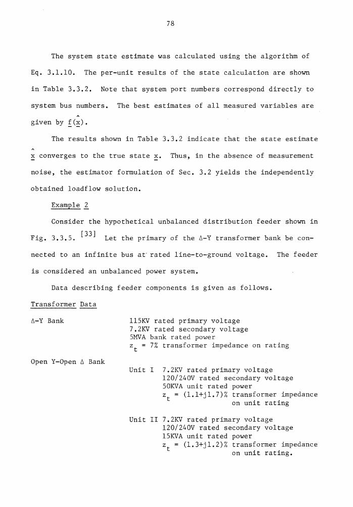
The system state estimate was calculated using the algorithm of
Eq. 3.1.10. The per-unit results of the state calculation are shown
in Table 3.3.2. Note that system port numbers correspond directly to
system bus numbers. The best estimates of all measured variables are
given by !C~).
The results shown in Table 3.3.2 indicate that the state estimate
x converges to the true state ~· Thus, in the absence of measurement
noise, the estimator formulation of Sec. 3.2 yields the independently
obtained loadflow solution.
Example 2 Consider the hypothetical unbalanced distribution feeder shown in
Fig. 3.3.5. ( 33 ] Let the primary of the 6-Y transformer bank be con-
nected to an infinite bus at· rated line-to-ground voltage. The feeder
is considered an unbalanced power system.
Data describing feeder components is given as follows.
Transformer Data
6-Y Bank
Open Y-Open 6 Bank
llSKV rated primary voltage 7.2KV rated secondary voltage SMVA bank rated power zt = 7% transformer impedance on rating
Unit I 7.2KV rated primary voltage 120/240V rated secondary voltage SOKVA unit rated power zt = (l.l+jl.7)% transformer impedance
on unit rating
Unit II 7.2KV rated primary voltage 120/240V rated secondary voltage lSKVA unit rated power zt = (l.3+jl.2)% transformer impedance
on unit rating.

79
Table 3.3.2. State estimate results.
P-MEASUREMENTS Port Actual Measured Estimated
Number p p p
1 -0.951 -0.951 -0.951 2 -0.500 -0.500 -0.500 3 0.550 0.550 0.550 4 0.000 o.ooo o.ooo 5 0.300 0.300 0.300 6 0.500 0.500 0.500
Q-MEASUREMENTS Port Actual Measured Estimated
Number Q Q g 1 -0.435 -0.435 -0.435 2 -0.185 -0.185 -0.185 3 0.130 0.130 0.130 4 0.000 0.000 o.ooo 5 0.180 0.180 0.180 6 o. 0_50 0.050 0.050
T-MEASUREMENTS From To Actual Measured Estimated Port Port T T T -- --
1 4 0.508 0.508 0.508 3 2 -0.154 -0.154 -0.154 5 6 -0.004 -0.004 -0.004 3 4 -0.395 -0.395 -0. 395 4 3 0.395 0.395 0.395 6 1 -0.416 -0.416 -0.416
U-MEASUREMENTS From To Actual Measured Estimated Port Port u u u -- --
1 4 0.254 0.254 0.254 3 2 0.024 0.024 0.024 5 6 -0.070 -0.070 -0.070 3 4 -0.154 -0.154 -0.154 4 3 0.178 0.178 0.178. 6 1 -0.107 -0.107 -0.107

80
Table 3.3.2. State estimate results (Continued).
E-MEASUREMENTS Port Actual Measured Estimated
Number E E E 2 1.100 1.100 1.100 3 0.999 0.999 0.999 4 0.929 0.929 0.929 5 0.919 0.919 0.919 6 0.919 0.919 0.919
STATE VARIABLES Port Actual Actual Estimated Estimated
Number v 0 v 0
1 1.05 o.o 1.05 o.o 2 1.100 -3.3 1.100 -3.3 3 0.999 -12.7 0.999 -12.7 4 0.929 -9.8 o. 929 -9.8 5 0.919 -12.3 0.919 -12.3 6 0.919 -12.2 0.919 -12.2

• ~
w . w . Vl .
~ -j
-I I o
i (")
I ix
N
_I
-~I
K! -
11' -
-1 I
I I
18
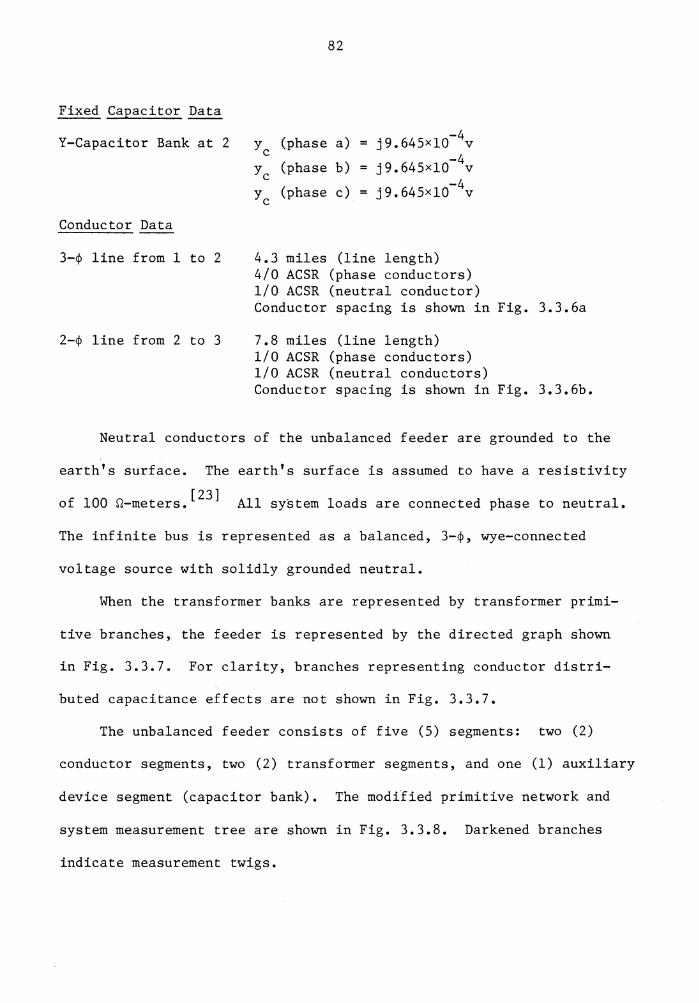
Fixed Capacitor Data
Y-Capacitor Bank at 2
Conductor Data
3-~ line from 1 to 2
2-~ line from 2 to 3
82
ye (phase a)
ye (phase b)
ye (phase c)
-4 j9.64SxlO v -4 j9.645xlO v -4 = j9.645xlO v
4.3 miles (line length) 4/0 ACSR (phase conductors) 1/0 ACSR (neutral conductor) Conductor spacing is shown in Fig. 3.3.6a
7.8 miles (line length) 1/0 ACSR (phase conductors) 1/0 ACSR (neutral conductors) Conductor spacing is shown in Fig. 3.3.6b.
Neutral conductors of the unbalanced feeder are grounded to the
earth's surface. The earth's surface is assumed to have a resistivity
of 100 Q-meters.[ 23 ] All system loads are connected phase to neutral.
The infinite bus is represented as a balanced, 3-~, wye-connected
voltage source with solidly grounded neutral.
When the transformer banks are represented by transformer primi-
tive branches, the feeder is represented by the directed graph shown
in Fig. 3.3.7. For clarity, branches representing conductor distri-
buted capacitance effects are not shown in Fig. 3.3.7.
The unbalanced feeder consists of five (5) segments: two (2)
conductor segments, two (2) transformer segments, and one (1) auxiliary
device segment (capacitor bank). The modified primitive network and
system measurement tree are shown in Fig. 3.3.8. Darkened branches
indicate measurement twigs.

83
a b c 0 0 0-l 74" I ( ~1 I 36"
n 42"
0 l -r 60' I ,,,..... -l
/7777777777/7/777///7//7 Fig. 3.3.6a. C9nductor spacing of 3-¢ line.
0 0-I 74" I r
42"
ol i
60'
777///7//////7777777//77 Fig. 3.3.6b. Conductor spacing of 2-¢ line.

84
Fig. 3.3.7. Primitive network of the unbalanced feeder.

13
Fig. 3.3.8. Modified primitive network and measurement tree.
00 \J1

86
A computer program to calculate the Y and Y admittance matrices tR mR
for a class of unbalanced power systems has been developed 1 • Power
systems given as input to the program must be such that all unbalanced
sources and loads are connected phase to ground.[ 34 J A program source
listing is made available through the Energy Research Group at Virginia
Polytechnic Institute and State University.
The unbalanced feeder of Fig. 3.3.5 is of the class of systems
acceptable as input to the aforementioned computer program. The Y tR
and Y admittance matrices of the unbalanced feeder were calculated. mR A set of measured variables was selected for the system and the
corresponding state variables identified. Hypothetical system loads
were assumed. Using the Y and Yt admittance matrices, a base case tR m
load flow solution of the unbalanced feeder was determined. Ports 1,
2, and 3 were taken as the slack ports.
Hypothetical measurements were obtained by introducing error to
system variables given by the base case loadflow •. A diagonal estimator
weighting matrix W was heuristically selected such that: (1) all load
measurements were weighted 1.0, (2) all conductor flow measurements
were weighted 0.25, and (3) all phase voltage magnitude measurements
were weighted 0.10.
The system state estimate was calculated using the algorithm of
Eq. 3.1.10. Ports 1, 2, and 3 were taken as swing ports; thus, their
voltages were known deterministically. The results of the state
lcomputer program was developed by D. L. Allen under sponsorship of the Energy Research Group at Virginia Polytechnic Institute and State Univ.

87
calculation, given in real units, are shown in Table 3.3.3. The best
estimates of all measured variables are given by!(~).
The results displayed in Table 3.3.3 indicate that the estimator
formulation of Sec. 3.2 yields a reasonable estimate of the true system
state when applied to a topologically unbalanced power system. These
results are only intended to demonstrate convergence to an acceptable
result.
Inasmuch as analysis of the estimator quality is considered
beyond the scope of this dissertation, accuracy of any given state
estimate is not considered.

88
Table 3.3.3. State calculation results.
P-MEASUREMENTS Port Actual Measured Estimated
Number P(KW) P(KW) P(KW)
4 200.000 198.500 198.784 5 200.000 199.500 197.745 6 200.000 199.000 198.903 7 30.000 30.500 30. 277 8 30.000 30.000 29. 771 9 30.000 29.500 30.851
11 0.000 0.000 -0.032 12 0.000 0.500 0.173 14 20.000 20.000 19.608 15 20.000 19.500 19.615 16 20.000 20.500 19.169
Q-MEASUREMENTS ' Port Actual Measured Estimated
Number Q-(KVAR) Q (KVAR) Q (KVAR) 4 300.000 300.000 300.001 5 300.000 295.000 297.290 6 300.000 304.000 299.997 7 60.000 59.500 60.323 8 60.000 60.000 59.356 9 60.000 59.500 59.085
11 0.000 0.500 0.830 12 0.000 0.000 -0.665 14 15.000 15.500 14.289 15 15.000 15.000 14.304 16 15.000 14.500 16.083

89
Table 3.3.3. State calculations results (Continued).
T-MEASUREMENTS From To Actual Measured Estimated Port Port T(KW) T(KW) T(KW) -- ---
4 7 60.570 60.500 60.080 5 8 64.331 64.000 61. 879 6 9 30.286 30.000 30.694 7 4 -60.001 -60.000 -60.020 8 5 -63.088 -63.000 -61.024 9 6 -30.203 -30.000 -30.884
U-MEASUREMENTS From To Actual Measured Estimated Port Port U(KVAR) U(KVAR) U(KVAR) -- --
4 7 17.561 17.500 19.980 5 8 59.135 59.000 55.025 6 9 10.550 10.500 10.200 7 4 -16.031 -16.000 -19.253 8 5 -57.507 -58.000 -54.907 9 6 -10 .• 522 -10.500 -10.209
E-MEASUREMENTS Port Actual Measured Estimated
Number E(KV) E(KV) E(KV)
11 7.018 7.018 7.009 12 6.829 6.820 6.850

90
Table 3.3.3. State calculation results (Continued).
STATE VARIABLES Port Actual Actual Estimated Estimated
Number V(KV) (deg.) V(KV) (deg.)
5 7.089 119. 352 7 .091 119.359 4 7.103 -0.633 7.102 -0.630 6 7.104 -120.558 7.105 -120.557 8 6.993 119. 502 7.001 119.503 7 7.068 -1. 218 7.064 -1.175 9 7.139 -120.476 7.137 -120.512
16 0.191 -155.326 0.191 -154.874 12 6.829 120.147 6.847 120.121 11 7.018 -2.148 7.010 -2.034 15 0.106 -60. 719 0.107 -60.663 14 0.108 118.276 0.109 118.297
1 66.401 90.000 66.401 90.000 2 66.401 -30.000 66.401 -30.000 3 66.401 -150.000 66.401 -150.000

CHAPTER 4. CONCLUSIONS AND RECOMMENDATIONS FOR FURTHER RESEARCH
State estimation of power systems has, until now, been limited
to balanced systems which can be represented by positive sequence
networks. The available literature offers no treatment of state
estimation of unbalanced power systems.
State estimation of unbalanced power systems must rely on
accurate network models representing power systems containing both
topological and load imbalances. The available literature offers
no such models.
4.1 Conclusions
A new network model has been developed which allows the calcula-
tion of state estimates for a class of unbalanced power systems. This
model is applicable to systems which exhibit both topological and load
imbalances.
The network model, representing power systems operating in steady
state, yields a set of complex algebraic equations in variables con-
venient for an accepted state estimation technique. Development of
the model equations appeal to multiport network theory and graph
theoretic principles.
The general methodology for obtaining multiport equations for
admittance networks has been presented. The general methodology
demonstrates port identification via imposition of a measurement tree.
91

92
Multiport equations for unbalanced power systems have been devel-
oped in two stages. First, the concept of power system segments has
been introduced. Rules have been established for decomposing power
systems into segments. The general methodology allows the formulation
of segment multiport equations.
The decomposition of power systems into segments is a new concept
which allows the formulation of equations which give conductor power
flows as a function of voltages in the phase voltage reference frame.
Rules for selecting segment measurement trees have been given such that
segment port variables correspond to measured and state variables needed
for state estimation.
The second stage of developing power system multiport equations
requires a scheme to examine· the topology of interconnected power
system segments. The concept of replacing segment primitives with
modified segment primitives has been introduced. The union of all
modified segment primitives forms a modified primitive network.
The modified primitive network is a new concept which allows the
passive components of an unbalanced power system to be represented by
an equivalent multiport network. Rules for selecting a system measure-
ment tree for the modified primitive network have been given such that
system port variables correspond to measured and state variables.
The general methodology for obtaining multiport equations for
admittance networks can be applied to the modified primitive network
with a system measurement tree specified. The methodology yields
equations which give system loads as a function of voltages in the

93
phase voltage reference frame.
Linear dependence among multiport equations has been examined.
Topological dependence and dependence among primitive equations has
been considered. Normalization of multiport equations has been
examined and a scheme to obtain per-unit segment primitive equations
is described.
State estimation of unbalanced power systems appeals to the
extended method of weighted least squares. An iterative algorithm
to determine the least squares estimate has been presented.
Rules are established which identify necessary state voltages
for unbalanced power systems. Estimator equations are formulated
from the multiport equations of the new network model. The concept
of port suppression is developed as a method to obtain estimator
equations as a function of state variables only.
Two examples have been offered that demonstrate the estimator
formulation. Example 1 considers the formulation when applied to a
well studied balanced power system. Example 2 demonstrates the esti-
mator formulation for a hypothetical unbalanced power system. The
resulting state estimates demonstrate that the new network model
can be employed to formulate a state estimator for power systems
exhibiting both topological and load imbalances.

94
4.2 Recommendations for Further Research
State estimation of unbalanced power systems will likely find
broadest application in the lower voltage (13.5 KV and below) distri-
bution systems. Rapid load variations are characteristic of power
distribution systems; hence, state estimates for such systems must be
updated rapidly. A typical distribution system can consist of
hundreds of nodes. It is essential that state estimate computation
time be minimized.
The voltage profile of a typical distribution system can vary
greatly over time. Per-unit voltage magnitudes can vary by more
than ten percent at some nodes. Per-unit load powers can differ by
several orders of magnitude. These considerations suggest that any
practical state estimator must be robust.
Experienced gained with the iterative algorithm of Eq. (3.1.10)
has shown that the convergence rate of the algorithm is sensitive to:
(1) the number of redundant measurements (m-n), (2) the initial state
x (starting voltage profile), and (3) the weighting matrix W. -o
Three areas for research directed towards the practical applica-
tion of state estimators for unbalanced systems will be discussed:
(1) normalization of multiport equations, (2) distributed state esti-
mation, and (3) recursive weighted least squares.
Normalization .9..f Hultiport Equations
The normalization scheme offered in Sec. 2.4 is a natural exten-
sion of normalization of balanced power systems. This scheme requires
a real base voltage for each segment and a real system base power.
95
Base voltages are most often chosen to be a segment phase-to-neutral
nominal voltage magnitude.
Often unbalanced systems contain segments having corresponding
phase ports with unequal' nominal phase-to-neutral voltage magnitudes.
Hence, corresponding phase port voltages, in per-unit, may differ
greatly. Clearly, the initial state x (starting voltage profile) for -o
the algorithm of Eq. 3.1.10 must be carefully specified so as to
agree with the per-unit scheme.
Additional research directed towards normalization of segment
multiport equations is recommended. The following per-unit trans-
formation is suggested.
Let the segment multiport equations be given in real units as
-I -m y v
m -m
Define segment per-unit currents and voltages as
where,
I -m pu
v -m pu
l E* I S* B -m B
= E-l V B -m
SB complex system base power
EB diagonal matrix of complex base port voltages.
It follows that
E* I B -m l E* Y E E-l V ~ B m B B -m
(4.2.1)
(4.2.2)
(4.2.3)
(4.2.4)

96
The per-unit segment multiport equations are given by
-I -m
where,
y 1 Et' y E m = s*B B m B pu
pu y
m pu v -m pu
(4.2.5)
The per-unit transformations of Eqs. (4.2.2) and (4.2.3) allow
port voltage angles and magnitudes to be normalized.
Distributed State Estimation
Implementation of a state estimator in a large unbalanced system
requires much computer storage capability. Computation time to deter-
mine the state estimate can be excessive. In large systems, measure-
ments telemetered to a central computing facility can require telemetry
channels many miles in length. Research directed towards distributed
processing of state estimates is recommended.
Consider the arbitrary large system shown in Fig. 4.2.1. Let the
system be arbitrarily divided into n overlapping subsystems so that
each system component belongs to one or more subsystems.
The system multiport equations are given by
-I -t
R (4.2.6)
Let each subsystem be considered as an independent system. Thus,
th multiport equations for the k subsystem can be determined and are
given by

97
. . .
Fig. 4.2.1. Large system divided into overlapping subsystems.

-I -~k
98
y v ~k -~k
(4.2.7)
(4.2.8)
Let a state estimator, as developed in Chapter 3, be assigned to each
subsystem. Assume measurements are available such that each subsystem
is observable.
Given the conditions setforth above, a state estimate can be
determined for each subsystem. A th
The state estimate ~k of the k sub-
system determines that subsystems state voltages V • The best esti--t
th A Rk mate of the k subsystem's port currents I is given by
-tRk
(4.2.9)
From Eq. (4.2.9), the best estimate of subsystem port admittance can
be determined. For the ith port of the kth subsystem, the best esti-
mate of port admittance is given by
(4.2.10)
where,
best estimate of load admittance at the ith port
best estimate of the ith port current
=best estimate of the ith port voltage.

99
Let the system multiport equations of Eq. (4.2.6) be partitioned
such that
where,
v -t RL
I vector of system reference port currents -tRS
V = vector of system reference port voltages -tRS
I vector of system load port currents -tRL
V vector of system load port voltages. -tRL
(4.2.11)
Let the system reference port voltages V be given. It remains -tRS
to determine the load port voltages V , in order to obtain the system -tRL
state.
From Eq. (4.2.10), it can be shown that
(4.2.12)
Each system load port can be found in one or more subsystems. Thus,
the best estimate of system load port currents I can be written as -tRL
where,
y v L -tRL
(4.2.13)
YL diagonal admittance matrix with diagonal entries of yk .• 1

100
Substituting I for I in Eq. (4.2.12) suggests that the best -tRL -tRL,..
estimate of load port voltages V can be obtained from -tRL
-Y V L -tRL
(4.2.14)
Solving Eq. (4.2.14) for V yields tRL
(4.2.15)
Equation (4.2.15) suggests that a state estimate can be obtained
by estimating system port admittances. Estimates of system port admit-
tances can be obtained from subsystem state estimates. The subsystem
state estimates are computed· independently and simultaneously in a
distributed processing scenario. Research directed towards optimal
subsystem identification is recommended.
Recursive Weighted Least Squares
Practical application of state estimators in distribution systems
will likely require many load measurements in order to obtain observ-
ability. The availability of many load measurements suggests that
recursive weighted least squares may offer a more time efficient and
robust estimator than the formulation given by Eq. (3.1.10).
A recursive least squares estimator would begin with a loadf low
solution obtained from only load measurements. Redundant conductor
power flow measurements and phase voltage magnitude measurements
would be processed into the state estimate recursively.

101
The state estimate would be obtained in a manner similar to
extended Kalman Filtering.[JS] Research directed towards development
of recursive weighted least squares estimators for unbalanced systems
is recommended.
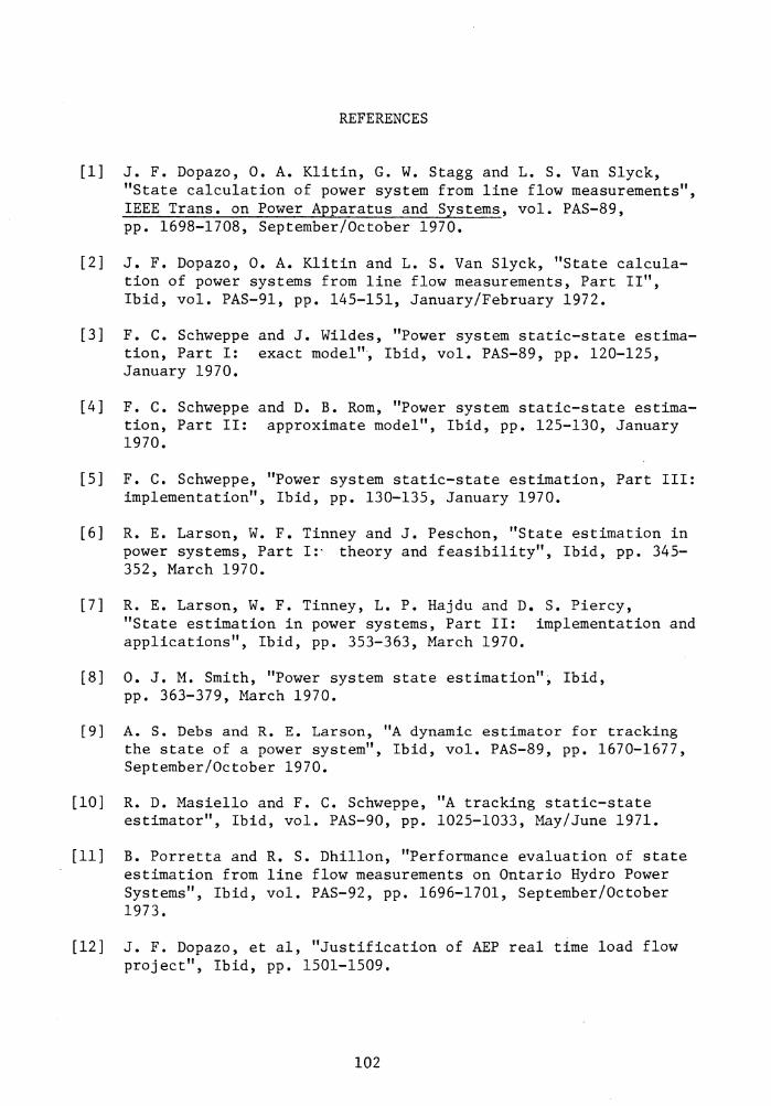
REFERENCES
[l] J. F. Dopazo, O. A. Klitin, G. W. Stagg and L. S. Van Slyck, "State calculation of power system from line flow measurements", IEEE Trans. on Power Apparatus and Systems, vol. PAS-89, pp. 1698-1708, September/October 1970.
[2] J. F. Dopazo, O. A. Klitin and L. S. Van Slyck, "State calcula-tion of power systems from line flow measurements, Part II", Ibid, vol. PAS-91, pp. 145-151, January/February 1972.
[3] F. C. Schweppe and J. Wildes, "Power system static-state estima-tion, Part I: exact model", Ibid, vol. PAS-89, pp. 120-125, January 1970.
[4] F. C. Schweppe and D. B. Rom, "Power system static-state estima-tion, Part II: approximate model", Ibid, pp. 125-130, January 1970.
[5] F. C. Schweppe, "Power system static-state estimation, Part III: implementation", Ibid, pp. 130-135, January 1970.
[6] R. E. Larson, W. F. Tinney and J. Peschon, "State estimation in power systems, Part I:· theory and feasibility", Ibid, pp. 345-352, March 1970.
[7] R. E. Larson, W. F. Tinney, L. P. Hajdu and D. S. Piercy, "State estimation in power systems, Part II: implementation and applications", Ibid, pp. 353-363, March 1970.
[8] O. J. M. Smith, "Power system state estimation", Ibid, pp. 363-379, March 1970.
[9] A. S. Debs and R. E. Larson, "A dynamic estimator for tracking the state of a power system", Ibid, vol. PAS-89, pp. 1670-1677, September/October 1970.
[10] R. D. Masiello and F. C. Schweppe, "A tracking static-state estimator", Ibid, vol. PAS-90, pp. 1025-1033, May/June 1971.
[11] B. Porretta and R. S. Dhillon, "Performance evaluation of state estimation from line flow measurements on Ontario Hydro Power Systems", Ibid, vol. PAS-92, pp. 1696-1701, September/October 1973.
[12] J. F. Dopazo, et al, "Justification of AEP real time load flow project", Ibid, pp. 1501-1509.
102

103
[13] A. S. Debs, "Estimation of steady-state power system model parameters", Ibid, vol. PAS-93, pp. 1260-1268, September/ October 1974.
[14] K. Srinivasan and Y. Robichaud, "A dynamic estimator for complex bus voltage determination", Ibid, pp. 1581-1588.
[15] W. D. Stevenson, Elements of Power Systems Analysis, McGraw-Hill, New York, 1975.
[16] N. Balabanian and T. A. Bickert, Electrical Network Theory, Wiley, New York, 1969,
[17] G. A. Campbell, "Mutual impedances of grounded circuits", Bell System Technical Journal, Oct., 1923, pp. 1-30.
[18] O. Mayr, "Einphasiger erdschluss und doppelerdschluss in vermaschten leitungsnetzen", Archiv flir Elektrotecknik, V. 17, Oct. 1926, pp. 163-173. ~
[19] J. R. Carson, "Wave propagation in overhead wires with ground return", The Bell System Technical Journal, V. 5, Oct. 1926, pp. 539-554.
[20] C. F. Wagner and R. D; Evans, Symmetrical Components", McGraw-Hill, New York, 1933.
[21] C. A. Gross, Power Systems Analysis, John Wiley and Sons, New York, 1979.
[22] P. Lorrain and D. Corson, Electromagnetic Fields and Waves, W. H. Freeman and Co., San Francisco, 1970.
[23] P. M. Anderson, Analysis of Faulted Power Systems, Iowa State Univ. Press, Ames, 1973.
[24] N. A. Demerdash, "Transients in power systems", Unpublished lecture notes, Virginia Polytechnic Institute and State University, 1976.
[25] W. A. Lewis, G. D. Allen and A. B. Chance, "Syrnrnetrical-component circuit constants and neutral circulating currents for concentric-neutral underground distribution cables", IEEE Trans. on Power Apparatus and Systems, vol. PAS-97, pp. 191-207, Jan./Feb. 1978.
[26] W. K. Chen, Applied Graph Theory Graphs and Electrical Networks, North Holland Publishing Co., New York, 1976.
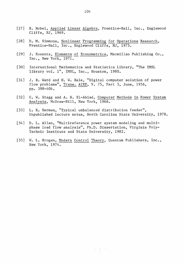
104
[27] B. Nobel, Applied Linear Algebra, Prentice-Hall, Inc., Englewood Cliffs, NJ, 1969.
[28] D. M. Simmons, Nonlinear Programming for Operations Research, Prentice-Hall, Inc., Englewood Cliffs, NJ, 1975.
[29] J. Konenta, Elements of Econometrics, Macmillan Publishing Co., Inc., New York, 1971.
[30] International Mathematics and Statistics Library, "The IMSL library vol. l", IMSL, Inc., Houston, 1980.
[31] J. B. Ward and H. W. Hale, "Digital computer solution of power flow problems", Trans. AIEE, V. 75, Part 3, June, 1956, pp. 398-404.
[32] G. W. Stagg and A. H. El-Abiad, Computer Methods in Power System Analysis, McGraw-Hill, New York, 1968.
[33] L. R. Herman, "Typical unbalanced distribution feeder", Unpublished lecture notes, North Carolina State University, 1978.
[34] D. L. Allen, "Multireference power system modeling and multi-phase load flow analysis", Ph.D. Dissertation, Virginia Poly-Technic Institute and State University, 1982.
[35] W. L. Brogan, Modern Control Theory, Quantum Publishers, Inc., New York, 1974.

APPENDIX A. YBUS FROM THE GENERAL METHODOLOGY
It is known from network theory that the nodal admittance matrix
YBUS is given by
It follows from Eq. (2.1.3) that
It follows from Eq. (2.1.4) that
-Q £
A BT = -A t t £
Solving Eq. (A.3) for B~ yields
Thus, from Eqs. (A.2) and (A.4) is follows that
Q = A-l A £ t £
(A. l)
(A. 2)
(A. 3)
(A. 4)
(A. 5)
Using Eq. (A.5), the multiport equations of Eq. (2.1.13) can be
rewritten as
-I -t (A. 6)
When a Lagrangian measurement tree is selected, it can be
shown that
u (A. 7)
105

106
where U is an identity matrix.
Hence, for a Lagrangian measurement tree, the multiport equations
are given by
-I t
where, the multiport admittance matrix is given by YBUS"
(A. 8)

APPENDIX B. THREE WINDING TRANSFORMER
Let all three winding transformers be represented by the equiva-
lent circuit shown in Fig. B.la, where
(B.l)
and
(B.2)
Three winding transformers can be represented as the three (3)
transformer primitive branches shown in Fig. B.lb. Transformer
primitive equations are given by
Il
I2 1 2 + 2
Y1 + a2y2 a3y3
I3
a2yly2 a3yly3 vl
2 -yly2 - a3y2y3 a2a3y2y3 v2
2 v3 a2a3y2y3 -yly3 - a2y2y3
(B.3)
107

108
-[}- 0 •
•
,
G) Y3
Fig. B.la. Three winding transformer.
G) 2
0 8
1 G) Q 3
Fig. B.lb. Primitive branches of three winding transformer.

APPENDIX C. TAP-CHANGING TRANSFORMER
Let a single phase tap-changing transformer be represented by the
equivalent circuit shown in Fig. C.la. It can be shown that the ideal
auto-transformer contained in Fig. C.la can be replaced by two linearly
dependent sources as shown in Fig. C.lb.
Tap-changing transformer segments can be constructed by the proper
interconnection of equivalent circuits. Note that all dependent
sources must appear in the system measurement tree. System ports
corresponding to these dependent sources must satisfy the following
port constraint equations. [34]
[ a* - l] 0 = -Ir. + a* Ii (C.l)
0 v + v. p 1.p (C. 2)
109

v
G) +
p
+
v p
I ) I p
Fig. C.la.
0
llO
a:l
I r
8 Tap-changing
0
Ii
transformer.
I. l.
G yt
Fig. C.lb. Equivalent circuit for tap-changing transformer.

The vita has been removed from the scanned document

STATE ESTIMATION OF UNBALANCED POWER SYSTEMS
by
Martin A. Wortman
(ABSTRACT)
A new network model has been developed which allows the calcula-
tion of state estimates for unbalanced electric power systems. This
model incorporates the effects of mutually coupled conductors, earth
return paths, unbalanced device configurations, and multiple voltage
references.
Development of the new model appeals to multiport network theory
and graph theoretic principles. Model equations are employed directly
to obtain least squares estimators in the phase-voltage reference
frame.
The concept of power system segments is introduced and segment
multiport equations are developed. The concept of power system
modified primitive networks is introduced and system multiport equa-
tions are developed.
Segment and system multiport equations are used to obtain a state
estimator formulation in variables suitable for practical systems
analysis.


![DEPARTMENT OF ELECTRICAL AND ELECTRONICS ENGINEERING · Prove Ybus =A t [y]A using singular t ransformation? (7) ii)Estimate the Ybus for the given network: Element Positive sequence](https://cdn.vdocuments.us/doc/165x107/5e50c2e2dcc0ac3eb07c0dcb/department-of-electrical-and-electronics-engineering-prove-ybus-a-t-ya-using.jpg)


