
USING BOTH MINOR AND MAJOR ARC DATA FOR
GLOBAL SURFACE WAVE DIFFRACTION TOMOGRAPHY
Anatoli L. Levshina;1, Michael P. Barmina, Michael H. Ritzwollera, and Jeannot Trampertb
aCenter for Imaging the Earth's Interior, Department of Physics, University of Colorado at
Boulder, Campus Box 390, Boulder, CO 80309, USA.
bDepartment of Geophysics, University of Utrecht, P.O. Box 80021 3508 TA Utrecht, The
Netherlands.
Keywords: Surface waves; Tomography; Phase velocity
Abstract
We extend a previously developed technique of global surface wave di�raction tomography
to accommodate major arc data. The addition of major arc data provides better spatial and
azimuthal resolution for regions with relatively poor coverage by minor arc paths. Examples
of Rayleigh wave phase velocity tomography at 50 and 100 s are presented. We show that
major arc data, which have a higher level of noise, nonetheless provide important additional
information about phase velocity distribution, especially for the Southern Hemisphere.
1. Introduction
This paper presents a further development of the tomographic techniques to invert surface
wave dispersion measurements to two-dimensional maps of phase or group velocities for a
set of periods. In the paper by Barmin et al. (2001), we described a method of surface
1Corresponding author
E-mail address: [email protected]
1

wave tomography based on geometrical ray-theory and largely ad hoc Gaussian smoothing
constraints. This method, which will be addressed here as Gaussian tomography, was used
in numerous studies of the regional Earth's structure (Levshin et al., 2001; Ritzwoller et al.,
2001). However, the ray-theory is essentially a high frequency approximation, and it is not
justi�ed in the presence of heterogeneities whose length-scale is comparable to the wavelength
of the wave [e.g., Woodhouse (1974), Wang & Dahlen (1995)]. For ray approximation to be
valid, the �rst Fresnel zone must be smaller than the scale-length of the heterogeneity.
This means that the lateral resolution of seismic models based on ray-theory is signi�cantly
limited.
The use of Born/Rytov's approximation for surface wave scattering (e.g., Woodhouse &
Girnius, 1982; Yomogida & Aki, 1987; Snieder & Romanowicz, 1988; Bostock & Kennett,
1992; Friederich et al., 1993, Friederich 1999; Meier et al., 1997; Spetzler et al., 2001, 2002;
Yoshizawa & Kennett, 2002; Snieder, 2002) has provided a theoretical framework for intro-
ducing a new technique for surface wave tomography which takes into account the �nite
width of the sensitivity zone around the great circle surface wave path (Ritzwoller et al.,
2002). The sensitivity zone corresponds approximately to the �rst Fresnel zone. Its maxi-
mum width increases with the epicentral distance and wavelength. This approach, which we
call di�raction tomography, was applied for global surface wave tomography and was also
used to construct a 3D global shear velocity model of the crust and upper mantle (Shapiro
& Ritzwoller, 2002). However, this approach was designed to use only minor arc data. Some
regions of the Earth, especially in the Southern hemisphere, cannot be e�ectively covered by
minor arc paths due to the sparse network of seismic stations. The use of major arc data in
tomographic inversions may signi�cantly improve the spatial resolution of the tomographic
maps and azimuthal coverage, which is important for studies of azimuthal anisotropy (Tram-
pert & Woodhouse, 2003). Minor and major arc observations have been previously used in
tomographic studies only in the great circle approximation (Trampert & Woodhouse, 1995,
1996, 2003; Ekstr�om et al., 1997). In this paper we extend di�raction tomography to ac-
commodate data from both arcs. To do this, we de�ne the zone of sensitivity for a major
arc path using the Born/Rytov's approximation. Due to the focusing e�ects at antipodes of
2

the source and the receiver, the form of this zone is more complicated than in the case of a
minor arc. We apply this approach to surface wave phase velocity measurements obtained
by Trampert & Woodhouse (1995) and estimate the improvements in spatial resolution and
the reliability of tomographic maps. We pay special attention to the Southern hemisphere,
and, particularly, the regions of the Southern Paci�c and Antarctica for which the coverage
by minor arc paths is still much worse than for the Northern hemisphere.
2. Fresnel Zones and Sensitivity Kernels for Major Arc Paths
The rule by which we de�ne the sensitivity zone for a given surface wave is quite simple.
Any point O on the surface of the globe which satis�es the inequality
j�S�O +�O�R ��S�Rj � �(T )=N (1)
belongs to this zone. Here �S�O and �O�R are the epicentral distances from epicenter to
the point O and from point O to the receiver (or vice versa). �S�R is the distance from
the source to the receiver along a minor/major arc depending on which kind of data is
considered (all distances are in km). �(T ) is the wavelength for a given period T , and N
is a constant. We use N = 8=3 recommended by Spetzler et al. (2001, 2002). Figure 1
(top) shows schematically how such a zone is de�ned on a tomographic grid. The zones of
sensitivity are shown in Figure 2 for minor and major arcs for 50 s and 100 s Rayleigh waves
for the PREM model of the Earth (Dziewonski & Anderson, 1981) at di�erent epicentral
distances.
We calculate the traveltime of surface waves from the source to the receiver as an integral
over the Earth's surface S:
tdi�q (T ) =ZSKq(r; T )v
�1
q (r; T )dS (2)
where Kq is the sensitivity kernel, and the vector r is a position vector on the Earth's surface.
Similar to Vasco et al. (1995) we assume that for a given epicentral distance the value of Kq
inside the sensitivity zone is constant and is inversely proportional to the width of the zone.
In the case, when this width is less than �=4, the sensitivity is truncated to the value at the
3

zero epicentral distance to avoid nonphysically large amplitude in the kernel. The sensitivity
kernel is zero outside the sensitivity zone and is normalized by the conditionZSKq(r; T )dS = 1: (3)
An example of the sensitivity kernel Kq as a function of an epicentral distance is shown
in Figure 1 (middle) and as a function of the distance from the great circle connecting source
and receiver in Figure 1 (bottom, the dashed line). Thisapproximation is compared with
Born/Rytov approximation (bottom, solid line).
Extending the de�nition of the sensitivity zone and kernels for major arc data allows us
to combine minor and major arc data for tomographic inversion of existing phase velocity
measurements.
3. Tomographic Inversion
0.0.1 Inversion technique
For tomographic inversion of the combination of minor and major arc data, we use the
method described in Barmin et al., (2001). This method is based on minimizing the following
objective function for an isotropic map m consisting of velocity perturbations relative to a
reference map:
(Gm� d)TC�1(Gm� d) + �2jjF (m)jj2 + �2jjH(m)jj2: (4)
Equation (4) is a linear combination of data mis�t, model roughness, and the amplitude of
the perturbation to the reference map. G is the forward operator that computes traveltime
from a map using equation (2). d is the data vector whose components are the observed
traveltime residuals relative to the reference map. C is the data covariance matrix or matrix
of data weights. F is a Gaussian spatial smoothing operator, and H is an operator that
penalizes the norm of the model in regions of poor path coverage. We note here that the
spatial smoothing operator is de�ned over a 2D tomographic map as follows
F (m) =m(r)�ZS
S(r; r0)m(r0)dr0 ; (5)
4

where S is a smoothing kernel:
S(r; r0) = K0 exp
�jr� r0j2
2�2
!(6)
ZS
S(r; r0)dr0 = 1; (7)
and � is the spatial smoothing width or correlation length. The vector r is a position vector
on the earth's surface. Values at spatial points between nodes are computed with bilinear
interpolation. The choice of the damping coe�cients � and � and the smoothing width � is
ad hoc. We typically apply spatial smoothing widths from 150 to 300 km.
As described in detail in Barmin et al. (2001), both the forward and inverse problems
stated above are solved on a grid. For global tomography, we usually use the 2��2� equatorial
grid.
0.0.2 Path density
The improvement in coverage of the Earth by surface wave paths with an addition of major
arc data may be presented in terms of path density. In the case of Gaussian Tomography,
we de�ned path density �(r) as the number of paths intersecting a square cell of the �xed
area with center at the point r. For di�raction tomography, this de�nition makes no sense,
because each path now is not a linear object but an area object. For this reason, we introduce
a pseudo path density �D(r; T ) by means of the formula
�D(r; T ) =Xq
Kq(r; T )�q (8)
where �q is the distance between source and receiver along a minor or major arc for the q-th
path, and Kq is the sensitivity kernel from equation (2). Summation is made for all paths for
which the point r is inside the sensitivity zone. This formulation approximates path density
in the limit when Fresnel zone becomes very narrow.
5

0.0.3 Resolution analysis
The solution of (4) describing an isotropic map of velocity perturbations is
m̂ = GTC�1�t =�GTC�1G
�m = Rm (9)
where matrix R
R =�GTC�1G+Q
��1
GTC�1G: (10)
is the resolution matrix. In this application, each row of R is a resolution map de�ning
the resolution at one spatial node. The resolution matrix is consequently very large and
the information it contains is somewhat di�cult to utilize. We attempt to summarize the
information in each resolution map by estimating a scalar quantity, which we call the spatial
resolution at each point of the grid. The spatial resolution of tomographic maps is deter-
mined here in a slightly di�erent manner than in Barmin et al. (2001). To estimate spatial
resolution, we �t a cone to each resolution map. This cone approximates the response of
the tomographic procedure to a �-like perturbation at the target node. The radius of the
cone base was taken in Barmin et al. (2001) as the value of the spatial resolution. It was
observed that in many cases the shape of response resembles a Gaussian bell, and therefore
the old estimate was biased to larger values of the spatial resolution. To eliminate this bias,
we introduce a new estimate of the spatial resolution as a parameter describing a Gaussian
bell function
A exp
�jrj2
2 2
!(11)
which is the best �t to a given resolution map. Here A is an amplitude at the target node.
The Gaussian function is de�ned on the base of the �tting cone enlarged by factor k. To
construct the optimal Gaussian bell, we convert negative values of the map to positive ones,
and discard as random noise all points of the map with amplitude less than A/m. We use
ad hoc values k = 1:2 and m = 10.
6

4. Data
0.0.4 Input data and data handling
Surface wave phase velocity measurements described by Trampert & Woodhouse (1995) were
used in the tomographic inversion. We limited ourselves to two periods, 50 s and 100 s, and
analyzed only Rayleigh wave data for these periods. In what follows, we will refer to minor
arc Rayleigh wave observations as R1 and to major arc observations of the same waves as
R2. The number of paths for the initial data set (R1, R2) is given in Table 1 (column 3). To
�nd possible outliers, we apply the two-stage procedure. At the �rst stage, we trace all paths
contained in raw data across maps predicted by the current global 3D model of Shapiro &
Ritzwoller (2002). Ray-tracing is done using the same algorithm as in tomographic inversion.
Figure 3 shows the relative traveltime residuals [(observed - predicted)/predicted] for the raw
data as a function of distance are shown in Figure 3. The mean values and �2:5�rms in the
window sliding along the epicentral distance are presented as well. The gaps in data at the
epicentral distances � � 160� � 200� and 340� � 360� are due to interference of minor and
major arc wave trains near the epicenter and its antipode, which makes phase measurements
in these ranges unreliable. A signi�cant number of outliers in data is evident. Data rejection
is based on statistics of phase velocity residuals, which are approximately proportional to
the relative traveltime residuals. Corresponding average values of rms for phase velocity
residuals are given in the Table 1 (column 4). Only paths with relative residuals between
�2:5 � rms are selected for further analysis. The numbers of selected paths are presented
in Table 1 (column 5).
At the second stage, we apply to these selected paths a consistency test (Ritzwoller &
Levshin, 1998). We check measurements along close paths with end points inside the same
cells of the size 110km�110km. We delete duplicates and reject inconsistent measurements.
After this test, the numbers of selected paths are reduced drastically as can be seen from
Table 1. This procedure allows us also to estimate the inherent errors of measurements.
Average rms values for the whole set of close paths with consistent travel times are given in
the column 6 of Table 1.
7
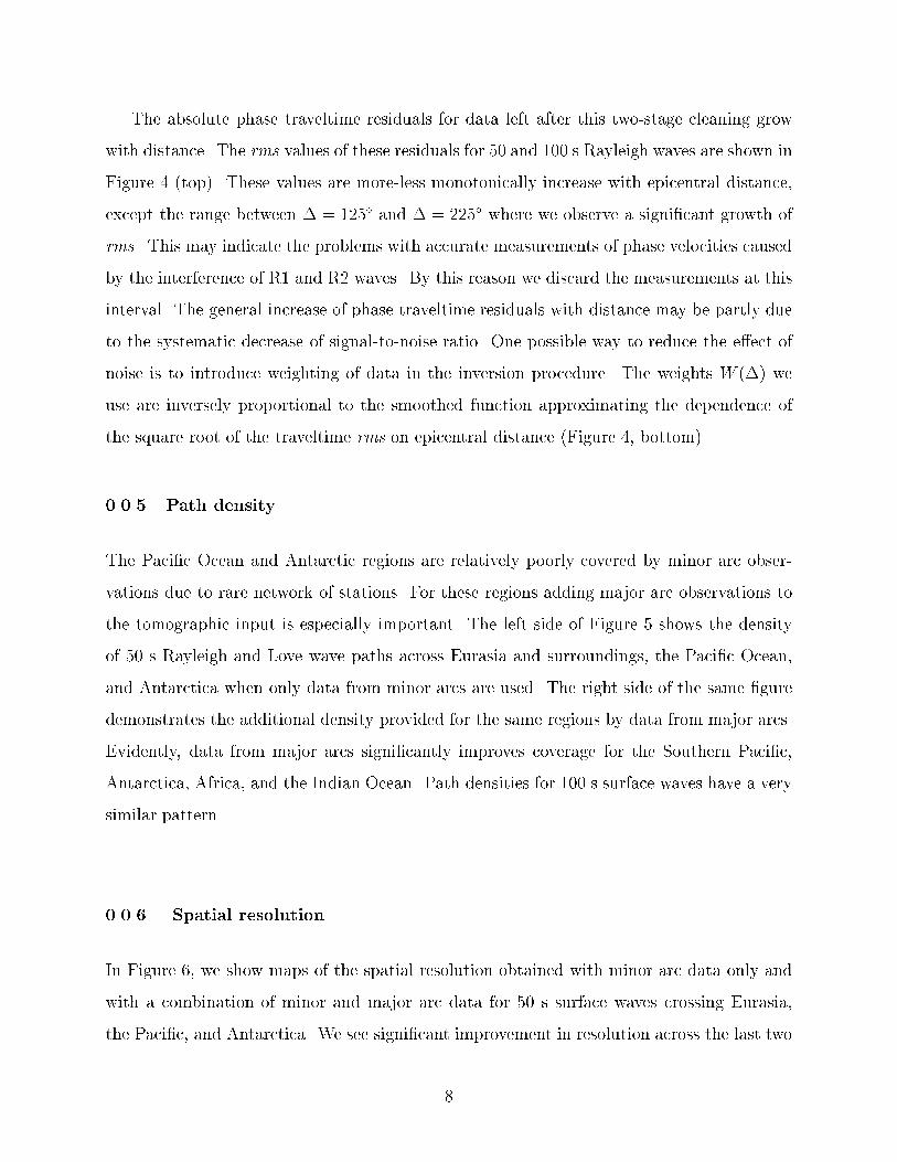
The absolute phase traveltime residuals for data left after this two-stage cleaning grow
with distance. The rms values of these residuals for 50 and 100 s Rayleigh waves are shown in
Figure 4 (top). These values are more-less monotonically increase with epicentral distance,
except the range between � = 125� and � = 225� where we observe a signi�cant growth of
rms. This may indicate the problems with accurate measurements of phase velocities caused
by the interference of R1 and R2 waves. By this reason we discard the measurements at this
interval. The general increase of phase traveltime residuals with distance may be partly due
to the systematic decrease of signal-to-noise ratio. One possible way to reduce the e�ect of
noise is to introduce weighting of data in the inversion procedure. The weights W (�) we
use are inversely proportional to the smoothed function approximating the dependence of
the square root of the traveltime rms on epicentral distance (Figure 4, bottom).
0.0.5 Path density
The Paci�c Ocean and Antarctic regions are relatively poorly covered by minor arc obser-
vations due to rare network of stations. For these regions adding major arc observations to
the tomographic input is especially important. The left side of Figure 5 shows the density
of 50 s Rayleigh and Love wave paths across Eurasia and surroundings, the Paci�c Ocean,
and Antarctica when only data from minor arcs are used. The right side of the same �gure
demonstrates the additional density provided for the same regions by data from major arcs.
Evidently, data from major arcs signi�cantly improves coverage for the Southern Paci�c,
Antarctica, Africa, and the Indian Ocean. Path densities for 100 s surface waves have a very
similar pattern.
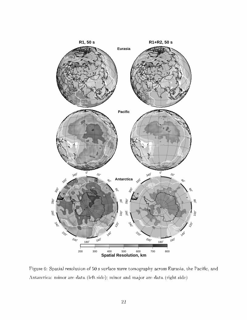
0.0.6 Spatial resolution
In Figure 6, we show maps of the spatial resolution obtained with minor arc data only and
with a combination of minor and major arc data for 50 s surface waves crossing Eurasia,
the Paci�c, and Antarctica. We see signi�cant improvement in resolution across the last two
8

regions when both types of data are used. The similar pattern is obtained for 100 s surface
waves.
5. Results of Tomographic Inversion
Results of the tomographic inversion of combined minor and major arc data [R1+R2] for
Rayleigh waves at periods 50 and 100 s are shown in the left sides of Figures 7 and 8. The
right side presents the results of tomography when only R1 data are analyzed. The same set
of parameters was used in both inversions. Three di�erent sets of maps are shown covering
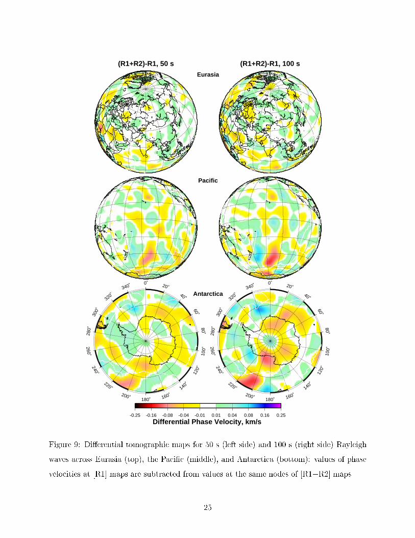
Eurasia and surroundings, the Paci�c, and Antarctica. Di�erential maps [(R1+R2) - R1]
(Figure 9) for the same regions demonstrate changes in phase velocities, which result from
the addition of major arc data. These changes are relatively small (in the range of �0:25
km/s, or 6 % ), but still essential, especially for the Southern Paci�c and Antarctica. The
e�ect of including major arc data in the tomographic data set can also be demonstrated by
comparison of changes in tomographic maps for two regions of the same size: the northern
part of the Northern Hemisphere for latitudes 45�N � 90�N and the southern part of the
Southern Hemisphere for latitudes 45�S � 90�S. The �rst region is well covered by R1
paths, and the second region is relatively poorly covered. Table 2 shows the correlation
between maps [R1 + R2], R1 for 50 and 100 s for these two regions. It is evident that for
the Northern Hemisphere changes in maps are signi�cantly smaller than for the Southern
Hemisphere. The correlation between two sets of maps is stronger, and the rms of the
absolute di�erence between the two maps is almost two times smaller for the North.
The question arises, does the addition of major arc data improve the maps providing more
accurate and more detailed information on phase velocity distribution across the globe, or
does it increase the noise in the obtained images? One of the ways to answer this question
is to examine the di�erence between the �t of minor arc data to maps obtained with these
data and to maps obtained with data from both arcs. Table 3 contains the information
about mis�t between observed and predicted traveltimes and group velocities for di�erent
combinations of Rayleigh wave maps and data sets for path covering the whole Earth. One
9

can see that addition of major arc data only slightly decreases the �t of observations from
R1 data to the prediction. Variance reduction relative to the reference model for R1 paths
traced across the [R1+R2] maps is of the order of 10% and is � 1:5 times less than with [R1]
maps. This could be explained by predominance of R1 data on R2 data. To evaluate if this
conclusion is valid also for data related only to the Southern Hemisphere where number of
R1 paths is relatively small, we selected R1 paths which are completely inside the Southern
Hemisphere. Corresponding data �ts are shown in Table 4. It is clear that even in this case
the mis�ts between minor arc data and the prediction from [R1+R2] maps and [R1] maps
are quite close. In general, the mis�t between R2 data and the prediction from the R1 maps
is noticeably higher than for the R1 data, The mis�t signi�cantly decreases when R2 data
are used in inversion. All this indicates that the addition of R2 data does not decrease the
quality of tomographic images.
6. Discussion and Conclusions
In the described approach, we solve a practical problem of inversion of numerous surface
wave dispersion measurements along minor and major arcs into reliable tomographic maps
of the surface wave velocities for given set of periods on the Earth's surface. Our tomographic
technique is based on several approximations:
(1) We accept the basic ideas of the Born/Rytov theory, an asymptotic theory for forward
scattering in the case when local inhomogeneities are much less than wavelengths. In reality
there is a wide spectrum of inhomogeneities (Chevrot et al., 1998), and the lower part of the
inhomogeneity spectrum does not comply with this constraint.
(2) We neglect path wander (Ritzwoller et al., 2002; Yoshizawa & Kennett, 2002), consider-
ing these e�ects at periods T � 50s as secondary in comparison with scattering e�ects.
(3) We simplify the expression for the sensitivity kernel in comparison with the one obtained
from the Born/Rytov theory (Spetzler et al., 2002). This approximation describes quite well
the main e�ects of forward scattering.
10

We applied this tomographic technique to the phase velocity data set obtained by Tram-
pert & Woodhouse (1995). The analysis of the major arc measurements indicates that they
are more noisy than the minor arc data and need to be weighted out. Nevertheless, our
tomographic simulations show that combining minor and major arc data in the frame of the
di�raction tomography may signi�cantly improve the spatial (and azimuthal) resolution of
data without degrading the data �t to predicted models of each type of observation. This is
especially true for the Southern hemisphere where the existing seismic network is sparse.
Acknowledgements
All maps were generated with the Generic Mapping Tools (GMT) data processing and display
package (Wessel and Smith, 1991, 1995).
11
References
Barmin, M.P., A.L. Levshin, and M.H. Ritzwoller, 2001. A fast and reliable method for
surface wave tomography, Pure Appl. Geophys., 158: 1351-1375.
Bostock, M.G. and B.L.N. Kennett, 1992. Multiple scattering of surface waves from discrete
obstacles, Geophys. J. Int., 108: 52-70.
Chevrot, S., J.P. Montagner, and R. Snieder, 1998. The spectrum of tomographic earth
models, Geophys. J. Int., 133: 783-788.
Dziewonski, A. M. and D. L. Anderson, 1981. Preliminary Reference Earth Model, Phys.
Earth. Planet. Int., 25: 297-356.
Ekstr�om, G., J. Tromp, and E.W.F. Larson, 1997. Measurements and global models of
surface wave propagation, J. Geophys. Res.: 102, 8147 - 8158.
Friederich, W., E. Wielandt, and S. Strange, 1993. Multiple forward scattering of surface
waves; Comparison with an exact solution and the Born single-scattering methods,
Geophys. J. Int., 112: 264-275.
Friederich, W., 1999. Propagation of seismic shear and surface waves in a laterally hetero-
geneous mantle by multiple forward scattering, Geophys. J. Int., 136: 180-204.
Levshin, A.L., M.H. Ritzwoller, M.P. Barmin, A. Villase~nor, 2001. New constraints on the
Arctic crust and uppermost mantle: Surface wave group velocities, Pn, and Sn, Phys.
Earth. Planet. Int. 123: 185-204.
Meier, T., S. Lebedev, G. Nolet, and F.A. Dahlen, 1997. Di�raction tomography using
multimode surface waves, J. Geoph. Res., 102(B4): 8255-8267.
Ritzwoller, M.H. and A.L. Levshin, 1998. Eurasian surface wave tomography: Group
velocities, J. Geoph. Res., 103: 4839-4878.
Ritzwoller, M.H., N.M. Shapiro, A.L. Levshin, and G.M. Leahy, 2001. Crustal and up-
per mantle structure beneath Antarctica and surrounding oceans, J. Geoph. Res.,
106(B12): 30,645-30,670.
12

Ritzwoller, M.H., N.M. Shapiro, M.P. Barmin, and A.L. Levshin, 2002. Global surface wave
di�raction tomography, J. Geoph. Res., 107 : B12, 2335,doi:10.1029/2002JB001777.
Shapiro, N.M. and M.H. Ritzwoller, 2002. Monte Carlo inversion for a global shear velocity
model of the crust and upper mantle, Geophys. J. Int., 151: 88-105.
Snieder, R. and B. Romanowicz, 1988. A new formalism for the e�ect of lateral hetero-
geneity on normal modes and surface waves { I: Isotropic perturbations, perturbations
of interfaces and gravitational perturbations, Geophys. J. R. astr. Soc, 92, 207-222.
Snieder, R., 2002. Scattering of surface waves, in Scattering and Inverse Scattering in
Pure and Applied Science, eds. R. Pike and P. Sabatier, Academic Press, San Diego:
562-577.
Spetzler, J., J. Trampert, and R. Snieder, 2001. Are we exceeding the limits of the great
circle approximation in global surface wave tomography?, Geoph. Res. Let. 28(12):
2341-2344.
Spetzler, J., J. Trampert, and R. Snieder, 2002. The e�ect of scattering in surface wave
tomography, Geophys. J. Int., 149: 755-767.
Trampert, J., and J. Woodhouse, 1995. Global phase velocity maps of Love and Rayleigh
waves between 40 and 150 seconds, Geophys. J. Int., 122: 675-690.
Trampert, J., and J. Woodhouse, 1996. High resolution global phase velocity distributions.
Geophys. Res. Lett., 23: 21-24.
Trampert, J., and J. Woodhouse, 2003. Global anisotropic phase velocity maps for funda-
mental mode waves between 40 and 150 seconds, Geophys. J. Int., 154: 154-165.
Vasco, D.W., J.E. Peterson, and E.L. Majer, 1995. Beyond ray tomography: Wavepath
and Fresnel volumes, Geophysics, 60: 1790-1804.
Wang, Z. and F.A. Dahlen, 1995. Validity of surface-wave ray theory on a laterally hetero-
geneous earth, Geophys. J. Int., 123: 757-773.
13

Wessel, P., and W.H.F. Smith, 1991. Free software helps map and display data, EOS, 72:
441.
Wessel, P., and W.H.F. Smith, 1995. New version of the Generic Mapping Tools released,
EOS, 76: 329.
Woodhouse, J.H., 1974. Surface waves in a laterally varying layered structure, Geoph. J.
R. astr. Soc., 37: 461-490.
Woodhouse, J. H. and T. P. Girnius, 1982. Surface waves and free oscillations in a region-
alized Earth model, Geoph. J. R. astr. Soc., 68: 653-673.
Yomogida, K., and K. Aki, 1987. Amplitude and phase data inversion for phase velocity
anomalies in the Paci�c Ocean basin, Geoph. J. R. astr. Soc., 88, 161-204.
Yoshizawa, K. and B.L.N. Kennett, 2002. Determination of the in uence zone for surface
wave paths, Geophys. J. Int., 149: 439-452.
14

Table 1. Number of paths before and after rejection of outliers, and after the consistency
test.
Period Wave Number of Rms, Ph. Vel. Number of Selected Number of Selected Rms, Ph. Vel.
sec Type Input Paths Res., m/s Paths (1st Stage) Paths (2nd Stage) Errors, m/s
50 R1 54168 22 49179 30543 6.7
50 R2 21347 26 14398 12672 4.6
100 R1 54168 26 50215 30446 8.7
100 R2 21347 30 15671 13681 3.2
Table 2. Comparison of tomographic maps for Northern and Southern regions obtained
with R1 and R1 + R2 data sets.
Region Period Wavetype Correlation Rms of di�erence
s Coe�cient m/s
45� � 90�N 50 Rayleigh 0.970 22
45� � 90�N 100 Rayleigh 0.968 23
45� � 90�S 50 Rayleigh 0.902 35
45� � 90�S 100 Rayleigh 0.821 44
15

Table 3. Mis�t between predicted and observed traveltimes and phase velocities
(all the World).
Period Map Type of Data Number Rms (traveltime) Variancey Rms (phase
s of Paths s Reduction,% velocity), m/s
50 R1+R2 R1+R2 39964 10.90 29.1 15.9
50 R1+R2 R1 27310 9.35 14.6 17.4
50 R1+R2 R2 12654 15.44 42.7 8.2
50 R1 R1 27310 9.02 20.4 16.8
50 R1 R2 12654 19.56 8.12 10.1
100 R1+R2 R1+R2 40483 10.27 23.1 19.2
100 R1+R2 R1 26852 8.93 11.0 20.4
100 R1+R2 R2 13631 10.87 35.1 6.2
100 R1 R1 26852 8.64 16.8 19.6
100 R1 R2 13631 17.86 -13.6 10.0
y Variance reduction is relative to predicted velocities from Shapiro & Ritzwoller (2002).
Table 4. Mis�t between predicted and observed traveltimes and phase velocities
(the Southern Hemisphere).
Period Map Type of Data Number Rms (traveltime) Variancey Rms (phase
s of Paths s Reduction,% velocity), m/s
50 R1+R2 R1+R2 5006 11.01 24.5 21.1
50 R1+R2 R1 3757 9.01 10.1 22.6
50 R1 R1 3757 8.31 25.1 23.5
100 R1+R2 R1+R2 5156 10.66 17.8 24.5
100 R1+R2 R1 3708 9.31 11.5 27.0
100 R1 R1 3708 8.66 23.5 25.5
y Variance reduction is relative to predicted velocities from Shapiro & Ritzwoller (2002).
16
-30
-20
-10
0
10
20
30
Wid
th,
o
0 30 60 90 120 150 180 210 240
∆ , o
∆S-R=240 o
0.0
0.1
0.2
0.3
0.4
0.5
Res
olut
ion
kern
el,
o
0 30 60 90 120 150 180 210 240
∆ , o
800 600 400 200 0 200 400 600 800
Distance from the ray (km)
Nor
mal
ized
sen
sitiv
ity k
erne
l
A
B
S R
RA SA
S RA SA R
A B
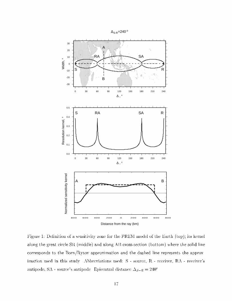
Figure 1: De�nition of a sensitivity zone for the PREM model of the Earth (top); its kernel
along the great circle SR (middle) and along AB cross-section (bottom) where the solid line
corresponds to the Born/Rytov approximation and the dashed line represents the approx-
imation used in this study. Abbreviations used: S - source, R - receiver, RA - receiver's
antipode, SA - source's antipode. Epicentral distance �S�R = 240�.
17

-40
-20
0
20
40
Wid
th,
o
0 20 40 60 80 100 120 140 160 180
∆S-R=30 o
-40
-20
0
20
40
0 40 80 120 160 200 240 280 320 360
∆S-R=190 o
-40
-20
0
20
40
Wid
th,
o
0 20 40 60 80 100 120 140 160 180
∆S-R=90 o
-40
-20
0
20
40
0 40 80 120 160 200 240 280 320 360
∆S-R=270 o
-40
-20
0
20
40
Wid
th,
o
0 20 40 60 80 100 120 140 160 180
∆S-R=170 o
-40
-20
0
20
40
0 40 80 120 160 200 240 280 320 360
∆S-R=350 o
S
RS
S R
S R
S R
SARA
S R
R
Figure 2: The zones of sensitivity for minor and major arcs for Rayleigh waves at periods
T = 100s (solid lines) and T = 50s (dashed lines) and indicated epicentral distances.
18

-5 -4 -3 -2 -1 0 1 2 3 4 5Relative Time Residual, %
2040
6080
100120
140160
180200
220240
260280
300320
340
Distance, o
-5 -4 -3 -2 -1 0 1 2 3 4 5
Relative Time Residual, %
2040
6080
100120
140160
180200
220240
260280
300320
340
Distance, o
14
1664
250500
1300
Figu
re3:
Shaded
plots
ofthedensity
ofrelative
traveltimeresid
uals
[(observed
-pre-
dicted
)/pred
icted]for
theentire
R1andR2phase
velocity
data
setpresen
tedversu
sepi-
central
distan
ce.Darker
shades
indicate
largernumber
ofresid
uals.
Thewhite
lines
show
therunningmean
,andtheblack
lines
show
�2:5�
.Density
isde�ned
asthenumber
of
residuals
insid
eeach
2��0:1%
cell.
19

0.4
0.5
0.6
0.7
0.8
0.9
1
0 50 100 150 200 250 300 350
50 s
100 s
5
10
15
20
25
30
35
0 50 100 150 200 250 300 350
+50 s
100 s
Epicentral Distance, °
Rm
s of
Tra
vel T
ime
Res
idua
ls, s
Epicentral Distance, °
Wei
ght
Figure 4: Rms of phase traveltime residuals for the cleaned data set as functions of epicentral
distance for 50 and 100 s Rayleigh waves (top). Weights as functions of epicentral distance
(bottom).
20

R1, 50 s
Eurasia
R2, 50 s
Pacific
0˚ 20˚
40˚
60˚80˚
100˚
120˚
140˚
160˚180˚
200˚
220˚
240˚
260˚
280˚
300˚
320˚340˚
0 50 100 200 300 500 800
Path Density
Antarctica
0˚ 20˚
40˚
60˚80˚
100˚
120˚
140˚
160˚180˚
200˚
220˚
240˚
260˚
280˚
300˚
320˚340˚
Figure 5: Pseudo-path density of 50 s surface waves across Eurasia, the Paci�c, and Antarc-
tica: minor arc data (left side); major arc data (right side). This approximates the number
of the rays in each 2� � 2� cell.
21
R1, 50 s
Eurasia
R1+R2, 50 s
Pacific
0˚ 20˚
40˚
60˚80˚
100˚
120˚
140˚
160˚180˚
200˚
220˚
240˚
260˚
280˚
300˚
320˚340˚
200 300 400 500 600 700 800
Spatial Resolution, km
Antarctica
0˚ 20˚
40˚
60˚80˚
100˚
120˚
140˚
160˚180˚
200˚
220˚
240˚
260˚
280˚
300˚
320˚340˚
Figure 6: Spatial resolution of 50 s surface wave tomography across Eurasia, the Paci�c, and
Antarctica: minor arc data (left side); minor and major arc data (right side).
22

R1+R2 50 s
Eurasia
R1
Pacific
0˚ 20˚
40˚
60˚80˚
100˚
120˚
140˚
160˚180˚
200˚
220˚
240˚
260˚
280˚
300˚
320˚340˚
-8.0 -4.0 -3.2 -2.6 -2.0 -1.3 -0.6 0.0 0.6 1.3 2.0 2.6 3.2 4.0 8.0
dC/C, %
Antarctica
0˚ 20˚
40˚
60˚80˚
100˚
120˚
140˚
160˚180˚
200˚
220˚
240˚
260˚
280˚
300˚
320˚340˚
Figure 7: Tomographic maps for 50 s Rayleigh waves across Eurasia (top), the Paci�c (mid-
dle), and Antarctica (bottom): minor and major arc data combined (left side); only minor
arc data used (right side).
23

R1+R2 100 s
Eurasia
R1
Pacific
0˚ 20˚
40˚
60˚80˚
100˚
120˚
140˚
160˚180˚
200˚
220˚
240˚
260˚
280˚
300˚
320˚340˚
-8.0 -4.0 -3.2 -2.6 -2.0 -1.3 -0.6 0.0 0.6 1.3 2.0 2.6 3.2 4.0 8.0
dC/C, %
Antarctica
0˚ 20˚
40˚
60˚80˚
100˚
120˚
140˚
160˚180˚
200˚
220˚
240˚
260˚
280˚
300˚
320˚340˚
Figure 8: Tomographic maps for 100 s Rayleigh waves across Eurasia (top), the Paci�c
(middle), and Antarctica (bottom): minor and major arc data combined (left side); only
minor arc data used (right side).
24
(R1+R2)-R1, 50 s
Eurasia
(R1+R2)-R1, 100 s
Pacific
0˚ 20˚
40˚
60˚80˚
100˚
120˚
140˚
160˚180˚
200˚
220˚
240˚
260˚
280˚
300˚
320˚340˚
-0.25 -0.16 -0.08 -0.04 -0.01 0.01 0.04 0.08 0.16 0.25
Differential Phase Velocity, km/s
Antarctica
0˚ 20˚
40˚
60˚80˚
100˚
120˚
140˚
160˚180˚
200˚
220˚
240˚
260˚
280˚
300˚
320˚340˚
Figure 9: Di�erential tomographic maps for 50 s (left side) and 100 s (right side) Rayleigh
waves across Eurasia (top), the Paci�c (middle), and Antarctica (bottom): values of phase
velocities at [R1] maps are subtracted from values at the same nodes of [R1+R2] maps.
25


