
Food Marketing Policy Center
Nonparametric Instrumental Variable Estimation in Practice
by Michael Cohen, Philip Shaw, and Tao Chen
Food Marketing Policy Center Research Report No. 111
November 2008
Research Report Series http://www.fmpc.uconn.edu
University of Connecticut Department of Agricultural and Resource Economics

Nonparametric Instrumental Variable Estimation inPractice†
Michael CohenUniversity of Connecticut
Philip ShawFairfield University
Tao ChenUniversity of Connecticut
October 20, 2008
†We thank: Joel Horowitz and Gautam Tripathi for valuable discussions about this research agenda. Wehave also benefitted from discussions and correspondence with Xiaohong Chen, Patrick Gagliardini, WhitneyNewey and Oliver Scaillet. Michael Cohen also thanks the Food Marketing Policy Center at the Universityof Connecticut for financial support for this research and the Booth School of Business at the University ofChicago for providing a great place to conduct the research.
1

Abstract
In this paper we examine the finite sample performance of two estimators one devel-oped by Blundell, Chen, and Kristensen (2007) (BCK) and the other by Gagliardini andScaillet (2007) (TIR). This paper focuses on the generalization and expansion of theseestimators to a full nonparametric specification with multiple regressors. In relation tothe classic weak instruments literature, we provide intuition on the examination of instru-ments relevance when the structural function is assumed to be unknown.
Simulations indicate that both estimators perform quite well in higher dimensions.This research also provides insights on the performance of bootstrapped confidence inter-vals for both estimators. We document that the BCK estimator’s coverage probabilitiesare near their nominal levels even in small samples as long as the sieve order of expansionis restricted. The coverage probability for the TIR estimator’s bootstrapped confidenceintervals are near their nominal levels even when the order of sieve approximation is large.These results suggest that in small samples the TIR estimator has a much smaller biasthen the BCK estimator but its variance is much larger. We provide two empirical ex-amples. One is the classic wage returns to education example and the other looks at therelationship of corruption and GDP to economic growth. Results here suggests that theimpact of corruption on growth depends nonlinearly on a countries level of development.
JEL codes: C13, C14, C15
Keywords: Nonparametric, Instrumental Variables, Information Regularized Estimators
2
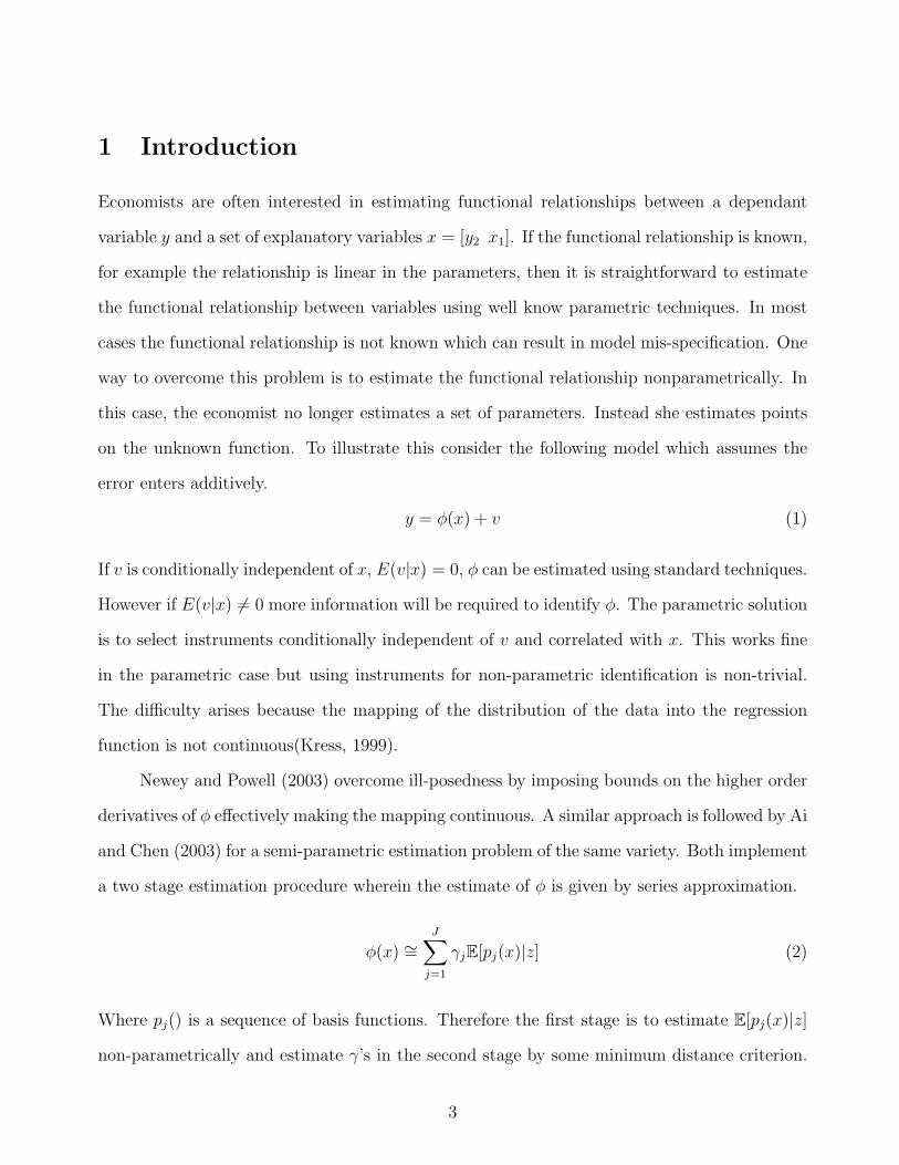
1 Introduction
Economists are often interested in estimating functional relationships between a dependant
variable y and a set of explanatory variables x = [y2 x1]. If the functional relationship is known,
for example the relationship is linear in the parameters, then it is straightforward to estimate
the functional relationship between variables using well know parametric techniques. In most
cases the functional relationship is not known which can result in model mis-specification. One
way to overcome this problem is to estimate the functional relationship nonparametrically. In
this case, the economist no longer estimates a set of parameters. Instead she estimates points
on the unknown function. To illustrate this consider the following model which assumes the
error enters additively.
y = φ(x) + v (1)
If v is conditionally independent of x, E(v|x) = 0, φ can be estimated using standard techniques.
However if E(v|x) 6= 0 more information will be required to identify φ. The parametric solution
is to select instruments conditionally independent of v and correlated with x. This works fine
in the parametric case but using instruments for non-parametric identification is non-trivial.
The difficulty arises because the mapping of the distribution of the data into the regression
function is not continuous(Kress, 1999).
Newey and Powell (2003) overcome ill-posedness by imposing bounds on the higher order
derivatives of φ effectively making the mapping continuous. A similar approach is followed by Ai
and Chen (2003) for a semi-parametric estimation problem of the same variety. Both implement
a two stage estimation procedure wherein the estimate of φ is given by series approximation.
φ(x) ∼=J∑j=1
γjE[pj(x)|z] (2)
Where pj() is a sequence of basis functions. Therefore the first stage is to estimate E[pj(x)|z]
non-parametrically and estimate γ’s in the second stage by some minimum distance criterion.
3

Blundell et al. (2007) is the only empirical application that has explored this type of estimator.
They estimate a shape invariant Engle curve system which admits a semi-parametric form.
In their model demographic scaling parameters enter parametrically and total expenditure is
treated as endogenous. Their semiparametric model and estimation technique is adapted from
Ai and Chen (2003). Hall and Horowitz (2005) present two methods for estimating φ based on
kernel and series approximating regressions and derive optimal convergence rates.
Severini and Tripathi (2006) explore identification issues with these models and note
that point wise identification can easily fail. Their work also provides intuition on how to
determine the identified part of the structural function φ. They examine the relationship
between identification of the structural function and identification of linear functionals and
uncover a connection between them.
Newey and Powell (2003) show that in their framework a condition needed for identifi-
cation is the completeness of the conditional distribution f(x|z). Severini and Tripathi (2006)
shows that completeness of the conditional distribution is equivalent to a correlation between
the model space and the instrument space. As we will show later, ill-posedness can be caused
by weak or irrelevant instruments in the sense that there is a very low correlation between the
model space and the instrument space.
Gagliardini and Scaillet (2008) and Darolles, Florens, and Renault (2006) propose esti-
mators which exploit information in the L2 norms of φ and its first derivative by regularizing
the second stage estimates with their Sobelev norm. This regularization penalizes the highly
oscillating components to achieve a continuous mapping. They call their estimators Tikhonov
Regularized estimators (TIR) after seminal work by Tikhonov (1963) that proposes this type
of regularization for ill-posed inverse problems such as the one studied in this literature.
A related strand of literature studies specification testing. In this strand two varieties
of specification questions are addressed. First Gagliardini and Scaillet (2007) use the non-
parametric estimation techniques described above to construct statistics that test the validity
of parametric specifications of econometric models. The test of Gagliardini and Scaillet (2007)
4

is carried out in the spirit of Hardle and Mammen (1993). The test statistic uses a inte-
grated square error distance metric that measures the distance between the parametric and
non-parametric specifications. Gagliardini and Scaillet (2007) construct this test statistic using
their Tikhonov regularized non-parametric estimate of φ. Horowitz (2006) tests the hypothesis
that φ belongs to some finite dimensional parametric family against a non-parametric alterna-
tive. His test does not require the estimation of φ explicitly. Therefore rendering a solution to
the ill-posed problem is avoided.
Because the test mentioned above is only reasonable when E[v|z] = 0 Horowitz (2008)
presents a test that examines whether the solution is smooth. This is reasonable because
non-existence of a solution is an extreme form of non-smoothness. Horowitz also points out
that even if a solution exists and is not smooth rejecting the model is still reasonable. This
argument calls upon economic theories that dictate many models such as demand or Engle
curves be smooth. Therefore rejection of non-smooth models is justified on two grounds, non
existence and economic mis-specification. Horowitz shows that it is impossible to construct
a uniformly consistent test on a unrestricted set of alternatives thus he restricts his test to
smooth or nonsmooth functions over the null and alternative hypothesis. This is a reasonable
restriction because in most economic applications the function, as guided by theory, is often
smooth is the sense of having s many square-integrable derivatives.
The purpose of this paper is to examine the use of the non-parametric estimators briefly
described above and provide evidence of finite sample performance while offering techniques to
estimate multidimensional φ’s for vector valued applications. We focus on the Blundell et al.
(2007) (BCK) and Gagliardini and Scaillet (2008) (TIR) estimators and verify their performance
in small samples. We explore the performance of bootstrap methods in the construction of
confidence intervals, as well as discuss instrument relevance and speak about issues surrounding
the estimation of partial effects all specifically in the context of these estimation techniques.
The paper is organized as follows. In the first section we will present the estimators and
discuss practical estimation issues including the extension to multiple dimensions. The second
5

section will discuss ill-posedness and how it relates to the literature on weak identification.
Thirdly we conduct monte carlo experiments and present results from these simulations. The
fourth section looks at two empirical applications. Finally concluding remarks are made along
with suggestions for future work.
2 The Estimators
In this section we present the estimator constructed by Blundell et al. (2007) and Gagliardini
and Scaillet (2007). Both methods used rely upon a minimum distance criteria that can be
posed in a very general framework. Take the following model:
y = φ(y2) + v (3)
Under the assumption that E(v|y2) 6= 0 estimation of φ(y2) by traditional nonparametric meth-
ods yields poor and meaningless results. Now assume we observe a variable z that satisfies the
following condition E(v|z) = 0. Taking expectations over Equation (3) we obtain the following
equation:
m(φ(y2), z) = E(φ(y2)|z)− E(y|z) = 0 (4)
In operator notation let T (φ) = E(φ(y2)|z) and r = E(y|z) so that we can write Equation (4)
as:
T (φ)(z)− r(z) = 0 (5)
The solution to Equation (5) is said to be well-posed if the solution exists, is unique, and
continuous in r. Ill-posedness occurs because T−1 need not be continuous. One approach to
dealing with ill-posedness is through regularization which is generally represented as follows:
φλ = argminφ‖T (φ)− r‖2 + λ‖φ‖ (6)
6

Both Blundell et al. (2007) and Gagliardini and Scaillet (2007) rely upon the method above
to estimate φλ. ‖φ‖ is the norm of the function and its derivatives, commonly referred to as
a Sobolev norm, used by both Blundell et al. (2007) and Gagliardini and Scaillet (2007). ‖φ‖
is a penalization matrix determined by the Sobolev norm of ‖φ‖, heretofore C, and a scaling
parameter λ. An estimate of φ can be found by minimizing ‖T (φ)−r‖2 subject to the constraint
that ‖φ‖ ≤ p. In practice the constraint on the penalization matrix may be unknown therefore
Equation (6) will be solved for a given value of λ as suggested by Blundell et al. (2007).
Gagliardini and Scaillet (2007) approximate the mean integrated squared error of their
estimator and propose that in practice one should choose a penalization parameter λ such
that the MISE is minimized. Although this practice is not theoretically justifiable data driven
methods for selection of the penalization parameter improve the finite sample performance of the
estimator as simulations conducted later show. Blundell et al. (2007) take a different approach
suggesting that one might choose various values of penalization parameters and display the
results for each choice.
The main difference between the TIR estimator and the BCK estimator is how each
component of Equation (6) is estimated. For example, Blundell et al. (2007) estimate both
T (φ) and r via sieve estimation while Gagliardini and Scaillet (2007) use a combination of sieve
estimation and kernel methods to obtain a solution to the empirical counterpart to Equation
(6). Both methods rely upon the calculation of the penalization matrix C. Blundell et al. (2007)
provide the following equation characterizing their calculation of the kp+1n × kp+1
n penalization
matrix C:
Cr =
∫[∇rΨk(y2, x1)]′[∇rΨk(y2, x1)]dy2 (7)
Ψk(y2, x1) is the complete set of basis functions which is N × kp+1n if x1 is a N × p matrix. As
in Blundell et al. (2007) one might choose r = 0 and r = 2 so that C is constructed as:
C =
∫[Ψk(y2, x1)]′[Ψk(y2, x1)]dy2 +
∫[∇2Ψk(y2, x1)]′[∇2Ψk(y2, x1)]dy2 (8)
7

The choice of the order of derivative should be chosen based upon the application at hand.
In the case of Blundell et al. (2007), they choose the order of derivative based upon the type
of underlying function they focus on estimating. In practice the derivative and integration is
with respect to the endogenous variable only leaving this matrix as a function of the exogenous
variables. One approach might be to calculate the value for the penalization matrix at the
mean values of the remaining exogenous variables. In monte carlo simulations the choice of
which point does not seem to make any quantitative difference. Blundell et al. (2007) show
that their estimator φBCK(y2, x1) has a closed form solution given by:
ΠBCKλ = (Ψ′B(B′B)−1B′Ψ + λC)−1Ψ′B(B′B)−1B′y (9)
For a single instrumental variable, B(z, x1) is a N × kp+1n complete set of basis functions. We
construct φBCK(y2, x1) by multiplying our N×kp+1n basis functions Ψk(y2, x1) by the kp+1
n vector
of coefficients ΠBCKλ . Similarly, Gagliardini and Scaillet (2007) show that their estimator also
has a closed form solution expressed as:
ΠTIRλ = (λNC +
1
NP ′P )−1 1
NP ′R (10)
P = E(Ψk(y2, x1)|z, x1) and R = Ω(z, x1)E(Ψk(y2, x1)|z, x1) where Ω(z, x1) is an optimal
weighting matrix. Gagliardini and Scaillet (2007) estimate both P and R by kernel methods.
2.1 Instrument Relevance
Classic foundational work by Nelson and Startz (1990) and Staiger and Stock (1997) documents
the importance of paying close attention to the quality of instruments with respect to their
relevance. When the function φ(x) is known to be linear in parameters, Staiger and Stock
8

(1997) show that an F-stat of 10 or greater on the instruments in the first stage regression is
needed to have confidence in point estimation and thus inference. Under an unknown φ(x), not
much is known regarding how one might characterize what Staiger and Stock (1997) refer to
as “weak instruments”. It is intuitive that estimation in the nonparametric case should require
more from the data and thus it should be true that the rule of thumb proposed by Staiger and
Stock (1997) should not uniformly apply to estimation methods under an unknown φ(x). With
respect to the estimation method proposed by Blundell et al. (2007), they describe what they
refer to as a sieve measure of ill-posedness:
τn ≡ supφ(y2)∈Υn:φ 6=0
√Eφ(y2)2√
EE[φ(y2)|z]2≤ 1
µkn
(11)
where µkn are the singular values of the matrix T ∗T . Defining T (φ)(·) = E[φ(y2)|z = ·] and
T ∗ is the adjoint operator of T . The singular values are particularly important as the rate of
the decay serves as a measure of instrument relevance. The slower the rate of decay the faster
the rate of convergence of the estimator. Ideally one estimates the values of µkn and examines
the rate of decay with respect to some benchmark. For example, if y2 and z are jointly normal
with correlation ρ then the rate of convergence of the singular values can be expressed as an
exponential function. Unfortunately, the rate of convergence depends upon the underlying
distribution of f(y2, z) which is unknown to the economist and the particular sieve being used.
One approach is to assume an underlying distribution for f(y2, z) and then see if there is an
optimal rate of decay for that distribution and particular basis function approximation. If
the performance of these estimators is independent of the type of basis function being used,
this might be a worthy approach. From this derivation a distance test can be derived for a
given distribution of data. Notice that for Equation (11) when z is replaced by y2, assuming
exogeneity of y2, then τn is identically 1. In practice we can estimate this value to see how
close it is to 1. If the instruments are less than perfect then the value for Equation (11) will
be away from 1. The problem is we don’t necessarily know how far from 1 is too far. To get
9

some idea of how this estimator is distributed Figure (1) shows the probability density of the
empirical analog to Equation (11) across three levels of correlation between the instrument z
and y2 under joint normality for cosine basis functions of the order five. From the plot we
can see that when the instruments are strong the estimator τn is distributed tightly around a
median value of 1.04. For γ = .5, τn is centered around a median value of 1.14 as compared
to a median value of 1.17 when the instruments are completely irrelevant (γ = 0). This is an
interesting result because it suggest that we could observe values of τn close to 1 even though
our instruments are completely irrelevant. From this, it seems that using this as a measure
of instrument relevance might not be terribly informative. However, it is not likely to observe
values for τn greater than 1.4 when γ = .5, so if large values of τn are observed in practice it
would certainly be an indicator of weak instruments.
3 Monte Carlo Simulations
3.1 Single Regressor Case
This section investigates the finite sample performance of the TIR and BCK estimators for a
single endogenous regressor over various functional forms and orders of approximation. The
data is generated by the following process, the joint density,
z
v
y2
d∼N
0
0
0
,
1 γ 0
γ 1 ρ
0 ρ 1
(12)
, and the functional relationship,
y = β0y∗2 + (1− β0) sin(απy∗2) + v (13)
10

Notice that α controls the frequency of the function and β0 the degree of linearity. Here
y∗2 = Φ(y2−y2σy2
). We allow α to vary which controls the “waviness” of the function in which case
the order of approximation should be higher in order to pick up on the higher frequency.
Tables (1) and (2) present coverage probabilities of the quantiles for the BCK and TIR
estimators respectively. Table (1) displays coverage probabilities for the second through seventh
order approximations of the regression function. It is clear that once the polynomial reach the
fourth order the confidence intervals contain 96 percent of the bootstrapped estimates or better.
On the other hand Table (2) displays the coverage probabilities for alternative forms of the data
generation process. Here the polynomial’s order of approximation is 6. Results here document
that the estimator performs uniformly well over the different permutations of the function. In
the next section we continue by investigating the case where our regression function has to
independent variates.
3.2 Multiple Independent Variables
In this section we increase the dimension of the estimation problem and investigate the finite
sample performance of the TIR and BCK estimators through Monte Carlo simulations. We
generate the data as follows:
z
v
y2
d∼N
0
0
0
,
1 γ 0
γ 1 ρ
0 ρ 1
(14)
The additional exogenous variable is x1d∼N(0, 1). We generate the dependent variable as follows:
y = β0y∗2 + (1− β0) sin(απy∗2) + β1x
∗1 + (1− β1) sin(απx∗1) + v (15)
Figures (1) and (2) portray a representative function in the top left, that has β0 = 0,
11

β1 = 0, and α = 2. Figure (1) plots the TIR estimate of the function. A first glace reveals
that the estimator picks up all the relevant curvature in the true function. Additionally, the
estimator also picks up the relevant scale. Subplot c. For this figure shows that the measurement
error is small particularly over the interior of the function, with larger error revealing itself on
the perimeter of the grid where the true model generates observations with lower probability.
Figure (2) plots the same set of diagrams for the BCK estimates of the true function. The BCK
estimator does a relatively good job picking up the contours in the interior of the function’s
support, However in subplot b of Figure (2) the estimator misses the true function with greater
regularity. A glance at subplot c. of this figure verifies that the estimator does well where it has
more information on the data generation process but comes up short and to a comparatively
greater extent than the TIR estimator.
Table (3) summarizes and supports the discussion of the preceding paragraph by providing
some metrics on relative performance of the estimators as compared to traditional sieve esti-
mates that do not account for the endogeneity. This table documents that the TIR estimates
have and smaller point wise bias however the variance of the TIR estimates are more than twice
that of the BCK estimates. The mean square error is also not surprisingly higher for the TIR
than the BCK estimates. We have provided a results appendix to the paper that provides more
such tables for small and larger sample sizes and various permutations of the parameters for
the dependant variable generation function. The findings are consistent over all the results. In
general we find that in smaller samples the TIR estimates have a significantly smaller bias than
the BCK estimates. On the other hand the BCK estimates have smaller variance that the TIR
estimates. The paper continues with two empirical examples.
4 Two Applications
In this section we present a classic text book example which is measuring the returns to ed-
ucation. It is clear that one may propose a relationship between wages and education as the
12

following:
log(wage) = φ(educ∗, X∗) + v (16)
It is widely accepted that E(v|educ) 6= 0 thus education is endogenous in the above equation.
If the function φ(educ,X) is known, then we can proceed with the usual two-stage least squares
estimation. In this example, we do not proceed under the assumption that this function is
known but instead rely upon the estimators above combined with bootstrapped confidence
intervals to provide some guidance as to what the function φ(educ,X) looks like. For the first
application, we assume only one additional exogenous variable is contained in X which we take
to be age. Thus the structural function we are interested in is φ(educ, age). The methods
outlined in section 2.1 for expanding the dimension of the estimator would allow us to include
more exogenous variables, for expositional purposes and graphical parsimony we proceed with
a bivariate example. We estimate the wage equation across a variety of values for kn.
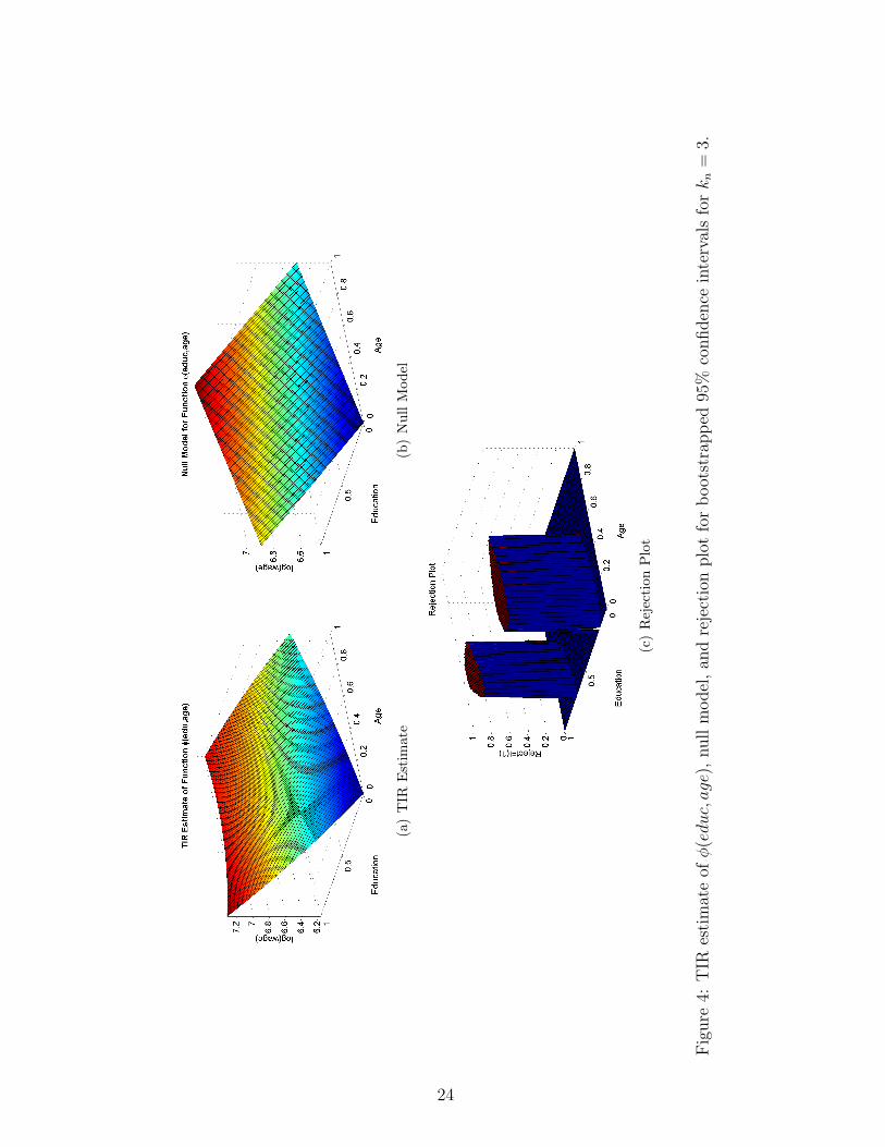
Figure (4) shows the TIR estimate of φ(educ∗, age∗). We transform values educ and age
where educ = Φ( educ∗− ¯educ∗
σeduc∗) and age = Φ(age
∗− ¯age∗
σage∗) to fall within the unit interval. This is
done because the estimator utilizes shifted Chebyshev polynomials as basis functions on the
unit interval. The null model is constructed as:
log(wage) = β0 + β1educ+ β2age+ v (17)
We obtain the values for the above coefficients from OLS and then plot the function for those
values. From this, we can then simply check to see if the model implied by the null model are
within the 95% confidence intervals constructed via the bootstrap. The rejection plot in Figure
(3) shows for which regions the null model is not within the confidence intervals. The results
suggest that we are able to reject the null model over a range of age and education values.
The TIR estimate reveals that the relationship between education, age, and wages are in fact
nonlinear over the range for which the linear model is rejected. In Figure (3) we report the
BCK estimates for kn = 3, 4 and TIR estimates for kn = 4. Although the BCK estimates show
13

a larger degree of curvature, we fail to reject the null model across all grid points consequently
we fail to reject the simple linear model.
This second economic relationship we examine that has been debated in the literature for
some time is the relationship between economic growth and corruption. From very early work
of Leff (1964), Huntington (1968), and Rose-Ackerman (1978) economists have been interested
in the relationship between economic growth and corruption. It was argued that corruption
could be good for growth or bad for growth depending upon various factors. Some economists
believed that corruption could be beneficial to growth because it can act as “speed money” while
other economists believe that it is detrimental to growth. Due to the nature of institutional
development it also thought to be true that corruption and growth are jointly determined thus
a measure of corruption is likely to be endogenous and thus classical assumptions as needed
in OLS break down. Mauro (1995) was the first to recognize this fact and correct for it under
the assumption that the relationship between corruption and growth is known. Shaw, Katsaiti,
and Jurgilas (2006) later shows that his results are uninformative due to irrelevant instruments
which actually result in unbounded confidence intervals. In the past, most empirical work while
acknowledging the endogeneity, has thought linearly about the relationship between economic
growth and corruption. Most models assume a standard linear framework and employ the
classical 2SLS. In this empirical example we estimate the relationship between growth and
corruption in a purely nonparametric framework allowing for initial conditions to enter the
model nonparametrically. Thus we estimate the following model:
growth = φ(cor, gdp70) + v (18)
We look at the average growth rate over the period of 1960-2004 (growth) using logarithmic
of gross domestic product in 1970 (gdp70) as initial conditions. We chose 1970 as the base year
only because it significantly increased our sample size which ends up as 96. The sample size is
quite small but both estimators can perform moderately well for a moderate choice of kn. We
14

also measure the average level of corruption (cor) over the period of 1980-1997. The data for
corruption was taken from Dreher, Kotsogiannis, and McCorriston (2007). The instrumental
variable we use is a measure of ethnolinguistic fractionalization in 1985.
Notice that practically speaking the BCK and TIR estimators produce very different
results. For the null model we present the unconditional mean of the growth rate across
countries. We reject the null over a certain range of corruption and initial conditions. For
this region we construct a contour plot in Figure (7) to get a better idea of what is going on
in this range. Notice that regardless of the initial conditions there is a negative and significant
effect of corruption on economic growth. One thing worth noticing is that the rate at which
corruption impacts growth differs depending upon the initial conditions of the country. For
example consider a country with initial conditions of .5. If corruption in that country increases
from .20 to .35 then the growth rate will fall by .5%. For a country with initial conditions
of approximately .73 the same increase in corruption would yield a 1% decrease in long-run
growth. Therefore the impact of corruption on economic growth depends upon a countries level
of development.
5 Conclusion
This research provides an exploration of recently developed methods for estimating functions
nonparametrically that are identified by instrumental variables. We provided a practical dis-
cussion of two similar estimators and introduced how they could be practically extended to
consider models with multiple regressions that enter a function in some unknown fashion. A
practical discussion of instrument relevance is provided that guides practitioners in their choice
of instruments in the context of the nonparametric instrumental variable estimation problem.
Monte Carlo simulations present a comparison of the finite sample properties of the two esti-
mators. We find that the TIR estimator has a much smaller bias then the BCK estimator but
its variance is much larger.
15

Two empirical applications are explored. The classic wage education example is presented
as a familiar context in which readers may evaluate the estimators. The second empirical appli-
cation showcases an example where the use of nonparametric instrumental variable estimators
may be used to provide important insights on questions that have, until now, been largely left
to the speculation of inflexible priors on model specification. Nonparametric methods prove
to be a useful way to conduct economic research without imposing dogmatic structure on new
economic problems. The importance of dealing with endogenously determined relationships is
of utmost importance to empirical practitioners and it is our hope that this research provides
a stepping stone to further adoption of these techniques by economists in all fields.
16

References
Ai, C., & Chen, X. (2003). Efficient Estimation of Models with Conditional Moment Restrictions
Containing Unknown Functions. Econometrica, 71 (6), 1795–1843.
Blundell, R., Chen, X., & Kristensen, D. (2007). Semi-Nonparametric IV Estimation of Shape-
Invariant Engel Curves. Econometrica, 75 (6), 1613–1669.
Darolles, S., Florens, J., & Renault, E. (2006). Nonparametric Instrumental Regression. Tech.
rep., GREMAQ, University of Social Science, Toulouse, France.
Dreher, A., Kotsogiannis, C., & McCorriston, S. (2007). Corruption around the world: Evidence
from a structural model. Journal of Comparative Economics, 35 (3), 443–466.
Gagliardini, P., & Scaillet, O. (2007). A Specification Test for Nonparametric Instrumental
Regresion. Tech. rep., University of Lugano and Swiss Finance Institute.
Gagliardini, P., & Scaillet, O. (2008). Tikhonov Regularization for Nonparametric Instrumental
Variable Estimators. Tech. rep., University of Lugano and Swiss Finance Institute.
Hall, P., & Horowitz, J. (2005). Nonparametric methods for inference in the presence of instru-
mental variables. The Annals of Statistics, 33 (6), 2904.
Hardle, W. K., & Mammen, E. (1993). Comparing nonparametric versus parametric regression
fits. The Annals of Statistics, 21 (4), 1926–1947.
Horowitz, J. (2006). Testing a Parametric Model Against a Nonparametric Alternative with
Identification Through Instrumental Variables. Econometrica, 74 (2), 521–538.
Horowitz, J. (2008). Specification Testing in Nonparametric Instrumental Variables Estimation.
Northwestern University, Department of Economics.
Huntington, S. P. (1968). Political Order in Changing Societies. Yale University Press, New
Haven, CT.
17

Kress, R. (1999). Linear Integral Equations. Springer.
Leff, N. (1964). Economic Development Through Bureaucratic Corruption. American Behav-
ioral Scientist, 8–14.
Mauro, P. (1995). Corruption and Growth. Quarterly Journal of Economics, 110 (3), 681–712.
Nelson, C. R., & Startz, R. (1990). Some Further Results on the Exact Small Sample Properties
of the Instrumental Variable Estimator. Econometrica, 58 (4), 967–76.
Newey, W., & Powell, J. (2003). Instrumental Variable Estimation of Nonparametric Models.
Econometrica, pp. 1565–1578.
Rose-Ackerman, S. (1978). Corruption: A Study in Political Economy. Academic Press, New
York, NY.
Severini, T., & Tripathi, G. (2006). Some Identification Issues in Nonparametric Linear Models
with Endogenous Regressors. Econometric Theory, 22 (02), 258–278.
Shaw, P., Katsaiti, M.-S., & Jurgilas, M. (2006). Corruption and Growth Under Weak Identi-
fication. Working papers 2006-17, University of Connecticut, Department of Economics.
Staiger, D., & Stock, J. H. (1997). Instrumental Variables Regression with Weak Instruments.
Econometrica, 65, 557–86.
Tikhonov, A. (1963). On regularization of ill-posed problems. In Dokl. Akad. Nauk SSSR, Vol.
153, pp. 49–52.
18

10% 25% 50% 75% 90% kn Jn0.96 0.36 0.94 0.38 0.92 2 100.98 0.42 0.97 0.43 0.97 3 100.97 0.97 0.98 0.97 0.96 4 100.97 0.99 1.00 1.00 0.98 5 100.99 1.00 1.00 1.00 1.00 6 101.00 1.00 1.00 1.00 1.00 7 10
Table 1: Coverage probabilities for BCK bootstrapped confidence intervals by quantile: N =100, ρ = .50, γ = .85, β0 = .5, α = 2, λ = 0
10% 25% 50% 75% 90% β0 α0.94 0.96 0.92 0.94 0.91 0.00 1.000.94 0.97 0.92 0.95 0.94 0.50 1.000.94 0.95 0.96 0.94 0.92 1.00 1.000.97 0.84 0.95 0.85 0.96 0.00 2.000.96 0.86 0.96 0.88 0.96 0.50 2.000.94 0.95 0.96 0.94 0.94 1.00 2.00
Table 2: Coverage probabilities for TIR bootstrapped confidence intervals by quantile: N = 100,ρ = .50, γ = .85, and kn = 6
19

Fig
ure
1:P
robab
ilit
ydis
trib
uti
onof
siev
em
easu
reof
ill-
pos
ednes
sτ n
forkn
=5
cosi
ne
bas
isfu
nct
ions.
20

(a)
Tru
eFu
ncti
on(b
)T
IRE
stim
ator
(c)
Squa
red
Dis
tanc
e
Fig
ure
2:E
stim
ated
funct
ion
vers
us
true
funct
ion
forN
=30
0,ρ
=.5
0,kn
=5,β
0=
0,β
1=
0,α
=2,
andγ
=.5
0.
21

(a)
Tru
eFu
ncti
on(b
)T
IRE
stim
ator
(c)
Squa
red
Dis
tanc
e
Fig
ure
3:E
stim
ated
funct
ion
vers
us
true
funct
ion
forN
=30
0,ρ
=.5
0,kn
=5,β
0=
1,β
1=
0,α
=2,
andγ
=.5
0.
22

Table 3: Performance of BCK (λ = 0) and TIR estimators by average pointwise Bias2, Var,and MSE
N=300, kn = 5, γ = .5, ρ = .5TIR BCK OLS
β0 = 0, β1 = 0Bias2 0.016 0.121 0.256Var 0.588 0.239 0.077
MSE 0.604 0.360 0.333
Table 4: Performance of BCK (λ = 0) and TIR estimators by average pointwise Bias2, Var,and MSE
N=1000, kn = 5, γ = .5, ρ = .85TIR BCK OLS
β0 = 0, β1 = 0Bias2 0.049 0.069 0.715Var 0.179 0.189 0.010
MSE 0.228 0.258 0.725
23
(a)
TIR
Est
imat
e(b
)N
ull
Mod
el
(c)
Rej
ecti
onP
lot
Fig
ure
4:T
IRes
tim
ate
ofφ
(educ,age)
,null
model
,an
dre
ject
ion
plo
tfo
rb
oot
stra
pp
ed95
%co
nfiden
cein
terv
als
forkn
=3.
24
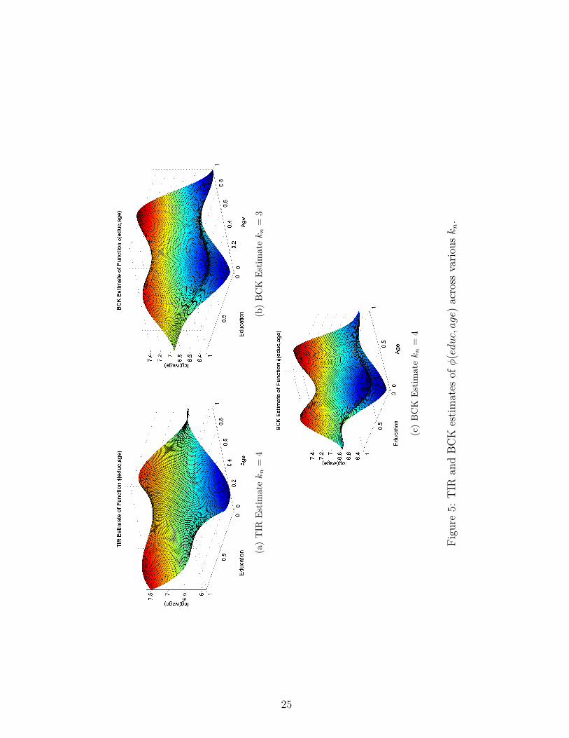
(a)
TIR
Est
imat
ek
n=
4(b
)B
CK
Est
imat
ek
n=
3
(c)
BC
KE
stim
ate
kn
=4
Fig
ure
5:T
IRan
dB
CK
esti
mat
esofφ
(educ,age)
acro
ssva
riou
skn.
25

(a)
BC
KE
stim
ate
(b)
Nul
lM
odel
(c)
Rej
ecti
onP
lot
Fig
ure
6:B
CK
(λ=.0
1)es
tim
ate
ofφ
(cor,gdp7
0),
null
model
,an
dre
ject
ion
plo
tfo
rb
oot
stra
pp
ed95
%co
nfiden
cein
terv
als
forkn
=3.
26

Fig
ure
7:C
onto
ur
Plo
tof
Gro
wth
onC
orru
pti
onan
dG
DP
70.
27

(a)
TIR
Est
imat
e(b
)N
ull
Mod
el
(c)
Rej
ecti
onP
lot
Fig
ure
8:T
IRes
tim
ate
ofφ
(cor,gdp7
0),
null
model
,an
dre
ject
ion
plo
tfo
rb
oot
stra
pp
ed95
%co
nfiden
cein
terv
als
forkn
=3.
28

6 Results Appendix
29

(a)
Tru
eFu
ncti
on(b
)T
IRE
stim
ator
(c)
Squa
red
Dis
tanc
e
Fig
ure
9:E
stim
ated
funct
ion
vers
us
true
funct
ion
forN
=30
0,ρ
=.5
0,kn
=5,β
0=
1,β
1=
0,α
=2,
andγ
=.8
5.
30

(a)
Tru
eFu
ncti
on(b
)B
CK
Est
imat
or
(c)
Squa
red
Dis
tanc
e
Fig
ure
10:
Est
imat
edfu
nct
ion
vers
us
true
funct
ion
forN
=30
0,ρ
=.5
0,kn
=5,β
0=
1,β
1=
0,α
=2,
andγ
=.8
5.
31

Table 5: Performance of BCK (λ = 0) and TIR estimators by average pointwise Bias2, Var,and MSE
N=300, kn = 5, γ = .5, ρ = .5TIR BCK OLS
β0 = 1, β1 = 0Bias2 0.018 0.115 0.250Var 0.571 0.232 0.074
MSE 0.588 0.347 0.324TIR BCK OLS
β0 = 1, β1 = 1Bias2 0.039 0.102 0.240Var 0.628 0.228 0.073
MSE 0.667 0.330 0.312
Table 6: Performance of BCK (λ = 0) and TIR estimators by average pointwise Bias2, Var,and MSE
N=1000, kn = 5, γ = .5, ρ = .85TIR BCK OLS
β0 = 1, β1 = 0Bias2 0.057 0.057 0.701Var 0.178 0.165 0.009
MSE 0.235 0.222 0.710TIR BCK OLS
β0 = 1, β1 = 1Bias2 0.048 0.081 0.713Var 0.185 0.192 0.011
MSE 0.233 0.273 0.725
10% 25% 50% 75% 90% kn Jn0.95 0.90 0.97 0.91 0.95 2 100.95 0.91 0.96 0.94 0.94 3 100.95 0.96 0.95 0.95 0.96 4 100.96 0.98 0.99 0.98 0.97 5 101.00 0.99 1.00 0.99 0.99 6 101.00 1.00 1.00 1.00 1.00 7 10
Table 7: Coverage probabilities for BCK bootstrapped confidence intervals by quantile: N =1000, ρ = .50, γ = .85, β0 = 1, α = 1, λ = 0
32

10% 25% 50% 75% 90% kn Jn0.94 0.92 0.97 0.91 0.94 2 100.95 0.94 0.98 0.93 0.95 3 100.95 0.98 0.99 0.99 0.96 4 100.98 1.00 1.00 1.00 0.98 5 100.99 1.00 1.00 1.00 0.99 6 101.00 1.00 1.00 1.00 1.00 7 10
Table 8: Coverage probabilities for BCK bootstrapped confidence intervals by quantile: N =100, ρ = .50, γ = .85, β0 = 1,α = 1, λ = 0
10% 25% 50% 75% 90% kn Jn0.88 0.86 0.06 0.92 0.28 2 100.96 0.94 0.94 0.89 0.89 3 100.97 0.99 0.94 0.97 0.92 4 100.99 1.00 1.00 0.98 0.96 5 100.99 1.00 1.00 0.99 0.99 6 101.00 1.00 1.00 1.00 1.00 7 10
Table 9: Coverage probabilities for BCK bootstrapped confidence intervals by quantile: N =100, ρ = .50, γ = .85, β0 = 0, α = 1, λ = 0
10% 25% 50% 75% 90% kn Jn0.88 0.00 0.94 0.00 0.95 2 100.92 0.00 0.95 0.00 0.96 3 100.94 0.94 0.95 0.93 0.95 4 100.95 0.98 0.99 0.97 0.96 5 101.00 0.99 0.99 0.98 1.00 6 101.00 1.00 1.00 1.00 1.00 7 10
Table 10: Coverage probabilities for BCK bootstrapped confidence intervals by quantile: N =1000, ρ = .50, γ = .85, β0 = .5, α = 2, λ = 0
33

FOOD MARKETING POLICY CENTER RESEARCH REPORT SERIES
This series includes final reports for contract research conducted by Policy Center Staff. The series also contains research direction and policy analysis papers. Some of these reports have been commissioned by the Center and are authored by especially qualified individuals from other institutions. (A list of previous reports in the series is available on our web site.) Other publications distributed by the Policy Center are the Working Paper Series, Journal Reprint Series for Regional Research Project NE-165: Private Strategies, Public Policies, and Food System Performance, and the Food Marketing Issue Paper Series. Food Marketing Policy Center staff contribute to these series. Individuals may receive a list of publications in these series and paper copies of older Research Reports are available for $20.00 each, $5.00 for students. Call or mail your request at the number or address below. Please make all checks payable to the University of Connecticut. Research Reports can be downloaded free of charge from our web site given below.
Food Marketing Policy Center 1376 Storrs Road, Unit 4021
University of Connecticut Storrs, CT 06269-4021
Tel: (860) 486-1927
FAX: (860) 486-2461 email: [email protected]
http://www.fmpc.uconn.edu


