Fast multipole accelerated boundary element method for solution of 3D scattering problems
Nail A. GumerovRamani Duraiswami
University of MarylandInstitute for Advanced Computer [email protected]
Fantalgo, [email protected]
Presented on Acoustics’08, Paris, France, July 2, 2008

Content
IntroductionFormulationBEM strategy for large problemsPeculiarities of the FMM usedfGMRES and FMM based preconditioningTest scattering problemsConclusion

Introduction
Several publications on BEM/FMMWideband FMM is a problem:
Low frequenciesHigh frequencies
As problem is solved iteratively, efficient BIE formulation and preconditioning are importantDifferent sources of errors should be consistently balancedBEM should be modified to fit memory/speed requirementsParallelization is relatively easy

kD022 =+∇ φφ k
D100050201
2005402
200.3704
6003020050
0.00410-5400100
kDD, mk, m-1f, kHz
microbubbles
fish school
speech
car vibrations
concert hall
Scaling with kD
The number of mesh vertices/panels, N, increases proportionally to (kD)2 so the minimal memory/speed complexity O((kD)2)The FMM error and complexity depends on the truncation numbers, p, which depend on kDEfficiency of translations is critical. If p2 is the size of representation and translation is performed with complexity O(pn), then the complexity of the FMM for simple shapes is O((kD)n) If n ≥ 4 the direct method for matrix-vector product is comparable or faster than the FMMUse of diagonal forms of translation operators provides translation exponent n=2, while some problems appear at low kDTo compute a problem with kD = 500 and several elements per wavelength one needs mesh size with 1 million vertices (2 million elements)Small kD cases may require also large meshes if the geometry of the problem is complex


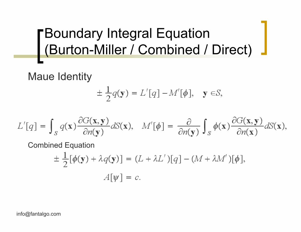
Boundary Integral Equation(Burton-Miller / Combined / Direct)
Maue Identity
Combined Equation
Basic notes concerning the use of the FMM in the BEM
Precomputations (singular elements, etc.) should be performed in O(N) or O(NlogN) computational and memory complexity“On the fly” computation of integrals should be computationally cheap as much as possibleSince the FMM is O(N) or O(NlogN) algorithm it is preferable to increase the size of the mesh and use low order integrals than use rough meshes and high order integrationIncrease of the mesh size is also preferable in terms of overall accuracy increase, since a larger mesh provides better shape approximation.
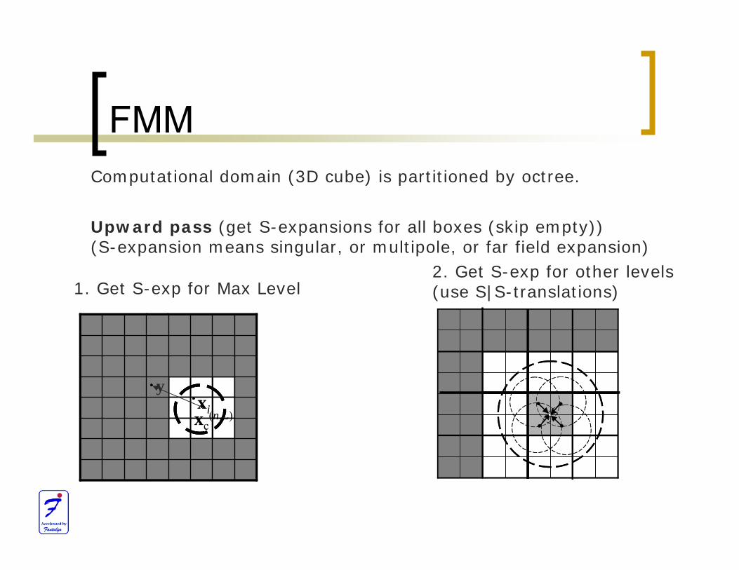
FMM
xixc(n,L)
y
Upward pass (get S-expansions for all boxes (skip empty))(S-expansion means singular, or multipole, or far field expansion)
Computational domain (3D cube) is partitioned by octree.
1. Get S-exp for Max Level2. Get S-exp for other levels(use S|S-translations)
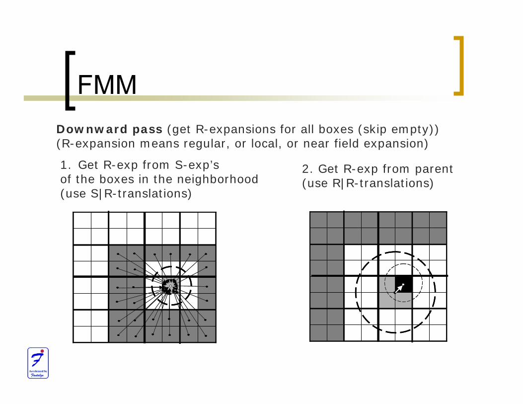
FMM Downward pass (get R-expansions for all boxes (skip empty))(R-expansion means regular, or local, or near field expansion)
1. Get R-exp from S-exp’sof the boxes in the neighborhood(use S|R-translations)
2. Get R-exp from parent(use R|R-translations)
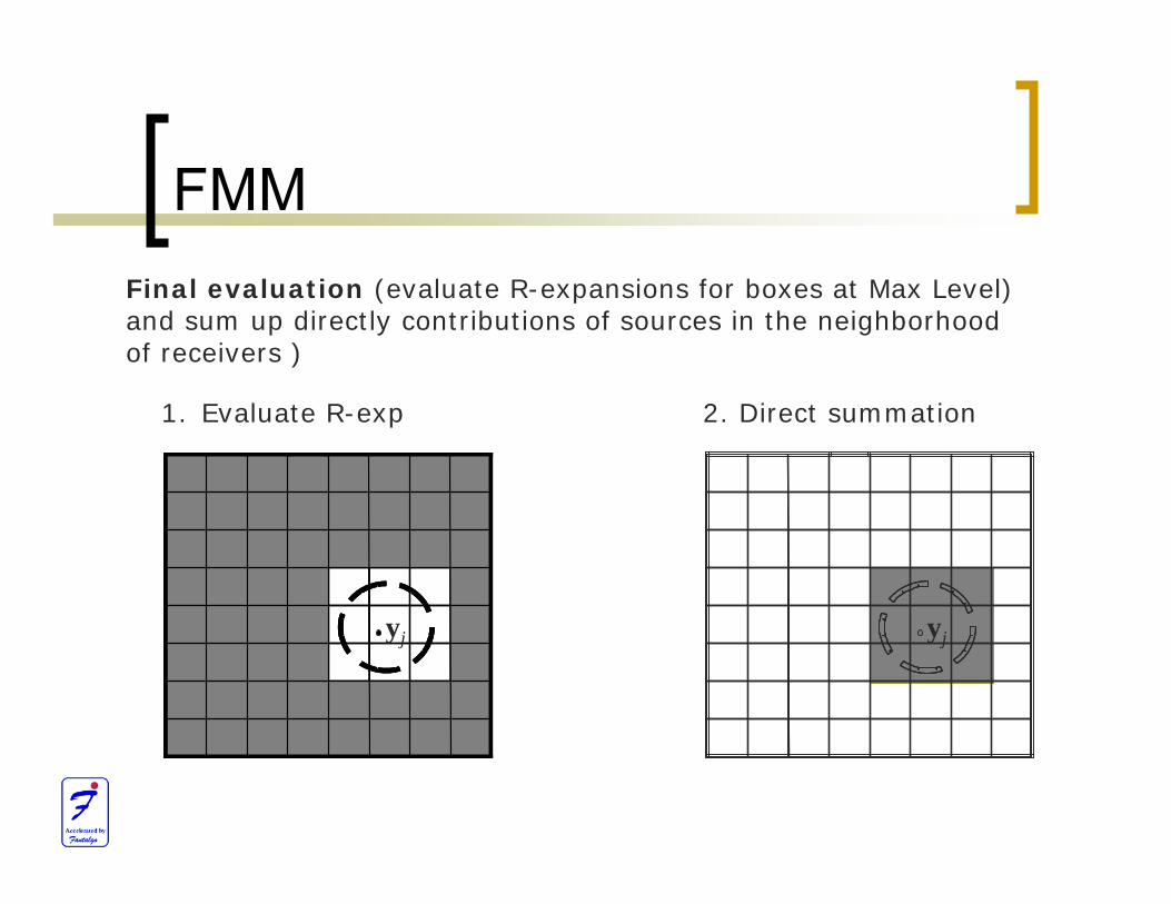
FMM Final evaluation (evaluate R-expansions for boxes at Max Level)and sum up directly contributions of sources in the neighborhoodof receivers )
1. Evaluate R-exp 2. Direct summation
yj yj

Wideband FMM
S S
S
S
S
S
FS
F
RR
R
R
R
R
F R
F
Sp Sp-1
Sp-1Sp
F|F
F|F
S|R
S|S
S|S
S|S
R|R
R|R
R|R
S
S S E
R
RRE
Sp-1
S
FF
F
Sp
F|F+i F|F
S|S
R|R
E|E
S|E E|R
R
F F
F
F|F+f
F|F
high frequency
low frequency
Cheng et al (2006) Present
S E REE|E
S|E E|R
S|S
R|RS|R
S S
S
S
S
S
FS
F
RR
R
R
R
R
F R
F
Sp Sp-1
Sp-1Sp
F|F
F|F
S|R
S|S
S|S
S|S
R|R
R|R
R|R
S
S S E
R
RRE
Sp-1
S
FF
F
Sp
F|F+i F|F
S|S
R|R
E|E
S|E E|R
R
F F
F
F|F+f
F|F
high frequency
low frequency
Cheng et al (2006) Present
S E REE|E
S|E E|R
S|S
R|RS|R


Translation methods and algorithm complexity
Matrix based translations are performed via the RCR-decomposition (Rotation-Coaxial translation-back Rotation), that has complexity O(p3) for p2
representationsConversion from representations via expansion coefficients to (and back) is performed with complexity O(p3)All other steps of the algorithm have complexity O(p2) or O((kD)2). Number of levels is O(logN).Overall complexity is O((kD)2 + α(ε) ((kD)3) with α<103).

fGMRES and FMM-based preconditioning
Ideal preconditioner M for solution of equation Ax=c is M=A-1
Approximate right preconditioner can be obtained via a program which solves Ay=b for given b with a matrix approximating AThis can be achieved using a few steps of unpreconditioned GMRES (inner iteration loop), while more accurate approximation of A is used in the outer loop of the fGMRESFMM speed substantially depends on the accuracyLow accuracy FMM can provide fast enough preconditioning

Tests for sphere
Incident wave ka=30
Typicall configuration:Comparing with analytical solution, which is available

Preconditioning
1.E-04
1.E-03
1.E-02
1.E-01
1.E+00
0 20 40 60 80 100 120Iteration #
Erro
r of R
esid
ual
Unpreconditioned
Preconditioned
0
20
40
60
80
100
120
0 20 40 60 80 100 120
Iteration #
Com
puta
tiona
l Cos
t
Converged (10-4)
Converged (10-4)
Unpreconditioned
Preconditioned
1.E-04
1.E-03
1.E-02
1.E-01
1.E+00
0 20 40 60 80 100 120Iteration #
Erro
r of R
esid
ual
Unpreconditioned
Preconditioned
0
20
40
60
80
100
120
0 20 40 60 80 100 120
Iteration #
Com
puta
tiona
l Cos
t
Converged (10-4)
Converged (10-4)
Unpreconditioned
Preconditioned
Neumann problem: ka=50 (kD=173), mesh: 202,808 panels, 101,402 vertices, overall accuracy: 5e-4,Time for mat-vec product in the outer loop: 9.75 sec, in the inner loop: 1.4 sec.Overall solution time: unpreconditioned ~ 1200 sec, preconditioned: ~ 400 sec(4 core PC, OMP parallelized algorithm)


Scaling with kDIn numerical experiiments kD varied in range 0.0001 ≤ kD ≤ 500For the largest kD mesh contained 1,500,002 vertices and 3,000,000 panels

Comparison with data available in the literature
2.87,7621,048,3462,096,688Present (2) (4 core)
2.73,820565,4961,130,988Present (1) (4 core)
4.854,2671,046,5281,046,528Tong et al (1 core)
M (GB)T (s)N (unknowns)# elements
Tong, M.S., Chew, W.C., and White, M.J. (2008)"Multilevel fast multipole algorithm for acoustic wave scattering by truncated ground with trenches,"
J. Acoust. Soc. Am., 123(5), 2513-2521.
kD=435, Robin problem, impedance=10-10i

Complex shapes
Nvert= 54,945Nelem=109,882
Nvert= 65,539Nelem=132,072
Nvert = 520,192Nelem= 1,038,336

Cars, etc.Recently this method wasIncorporated into commercialproducts
(Fantalgo, LLC: BEM/FMM)(ESI group: VA One)
Screen shot of the ESI VA One interface:Courtesy of the ESI Group
Conclusion
Practical acoustical scattering problems require wideband computations for kD in range 10-4-103 and meshes with up to millions elementsSuch problems can be solved by contemporary PCs which employ advanced algorithms, such as FMM and use advantage of multicorearchitecturesFMM based preconditioning enable speed up of solution several times and substantially reduce memoryUse of Burton-Miller (or combined) BIE is important to handle nearly resonance cases and high frequency modes (substantially accelerate convergence)Algorithm is scaled in complexity as (kD)2.4 or so at large kD<500.It is important to provide stabilization of some numerical procedures for the present algorithm. Additional research is needed to obtain stable methods for high kD.