a fast multipole dual boundary element method for the … · a fast multipole dual boundary element...

Copyright © 2011 Tech Science Press CMES, vol.72, no.2, pp.115-147, 2011

A Fast Multipole Dual Boundary Element Method for theThree-dimensional Crack Problems

H. T. Wang1,2 and Z. H. Yao3

Abstract: A fast boundary element solver for the analysis of three-dimensionalgeneral crack problems is presented. In order to effectively model the embeddedor edge cracked structures a dual boundary integral equation (BIE) formulation isused. By implementing the fast multipole method (FMM) to the discretized BIE,structures containing a large number of three-dimensional cracks can be readilysimulated on one personal computer. In the FMM framework, a multipole expan-sion formulation is derived for the hyper-singular integral in order that the multipolemoments of the dual BIEs containing the weakly-, strongly- and hyper-singular ker-nels are collected and translated with a unified form. In the numerical examples, theaccuracy of the proposed method for the evaluations of both the crack opening dis-placement (COD) and stress intensity factor (SIF) is tested, and its performance inboth the memory consumption and solution time in comparison with several otheralgorithms is investigated. The results are shown to demonstrate the effectivenessof this method for large-scale crack problems.

Keywords: dual boundary element method, fast multipole, large-scale, crackopening displacement, stress intensity factor

1 Introduction

The main attractive feature of the boundary element method (BEM) for the anal-ysis of linear elastic fracture mechanics (LEFM) is that only the boundary of theanalyzed domain needs to be discretized (Cruse 1996). This results not only in thesimplification of the crack meshing process, but also in a reduction of the degreesof freedom with respect to other numerical methods. In addition, the BEM pro-vides an efficient way to deal with the inherent nature of singularity at the crack tip

1 Corresponding author. Tel.: + 86 10 6278 4824; fax: + 86 10 6279 7136. Email address:[email protected] (H. Wang)

2 Institute of Nuclear & New Energy Technology, Tsinghua University, Beijing, 100084, P. R. China3 School of Aerospace, Tsinghua University, Beijing, 100084, P. R. China

116 Copyright © 2011 Tech Science Press CMES, vol.72, no.2, pp.115-147, 2011

via special treatments on only the crack tip boundary elements. Direct applicationof the displacement BEM to crack problems leads to a degenerated system matrixwhen two crack surfaces coincide. To overcome this mathematical difficulty, sev-eral techniques have been developed in the last several decades, including the crackGreen’s function method (Snyder and Cruse 1975), the displacement discontinu-ity method (Weaver 1977) and the multi-region method (Blandford, Ingraffea andLiggett 1981). The dual boundary element method (DBEM) is a novel techniquethat provides a single-region formulation for the analysis of general crack prob-lems. The DBEM was first introduced for the analysis of two-dimensional crackproblems by Portela and Aliabadi (1992) and three-dimensional crack problems byMi and Aliabadi (1992). This technique was then extensively studied and success-fully applied to a wide range of fracture mechanics problems (Portela, Aliabadi andRooke 1993, Mi and Aliabadi 1994, Chen and Chen 1995, Salgado and Aliabadi1996, Young 1996, Aliabadi 1997, Cisilino and Aliabadi 1997 and 2004, Chen,Chen, Yeih and Shieh 1998, Wilde and Aliabadi 1999, Partheymüller, Haas andKuhn 2000, Burczynski and Beluch 2001, Chao, Chen and Lin 2001, Albuquerque,Sollero and Aliabadi 2004, Purbolaksono and Aliabadi 2005, Kebir, Roelandt andChambon 2006).

Conventionally, the system matrix denoted by [A] arising from the BEM is fully-populated. This feature poses a serious challenge to the BEM since to solve theequation system [A]{X} = {B} by use of standard direct or iterative solvers, a com-putational cost of O(N3) or O(N2) is required, where N is the number of unknowns.In order to improve the efficiency of the BEM, much effort has been devoted to theimplementation of fast algorithms to the BEM solutions. Of particular interest wasthe fast multipole method (FMM) originally proposed by Rokhlin (1985) for clas-sical potential theory. The FMM has been successfully extended for the fast BEMsolutions for large-scale problems in the area of elasticity (Fu, Klimkowski, Rodinand colleagues 1998, Popov and Power 2001, Takahashi, Nishimura and Kobayashi2003, Liu, Nishimura, Otani and colleagues 2005, Wang and Yao 2005, Liu 2006,Sanz, Bonnet and Dominguez 2008, Wang, Hall, Yu and Yao 2008, Wang and Yao2008). A comprehensive review can be found in the literature (Nishimura 2002).

For the fast multipole BEM solutions of crack problems, we categorize recent in-vestigations into two groups according to the dimensional cases. One group con-sists of researches concerning two-dimensional cracks. Helsing (1999) and Hels-ing and Jonsson (2002) used the FMM accelerated BEM to treat two-dimensionalmany elastic cracks and demonstrated the efficiency of the proposed algorithms inlarge scales. Englund (2006) combined the FMM and a modified integral equationformulation to compute accurately the stress field in a two-dimensional finite edge-cracked domain. Liu (2008) developed a new fast multipole formulation for the hy-

A Fast Multipole Dual Boundary Element Method 117

persingular BIE in conjunction with the DBEM to deal with two-dimensional multi-domain elastostatic problems with inclusions and cracks. In his study, the crackis discretized with piecewise constant boundary elements. Wang and Yao (2006)proposed a fast multipole DBEM formulation and a special crack-tip element forthe two-dimensional general fatigue crack growth problems. Another group of pa-pers contribute to the fast BEM solutions of three-dimensional crack problems.Nishimura, Yoshida and Kobayashi (1999) proposed a FM-BEM based on the ef-ficient solid harmonic expansion formulation of the hypersingular kernels to solvethree-dimensional many crack problems in an infinite domain for the Laplace equa-tion using piecewise constant elements. Then Yoshida, Nishimura and Kobayashi(2001) applied the FMM-accelerated Galerkin BEM to three-dimensional elasticcrack problems in an infinite domain using piecewise linear elements. Lai andRodin (2003) developed a FM-BEM in conjunction with a weakly singular kernelto solve three-dimensional many crack problems in an infinite domain. In theirwork, the quadratic elements are used in order to get better results in comparisonwith linear or constant elements.

In addition to the FMM, another fast algorithm increasingly used recently for elas-tic crack problems is the Adaptive Cross Approximation method (ACA) proposedby Bebendorf and Rjasanow (2003). The ACA is an algebraic method whose ap-proximation is based only on the knowledge of indivisual matrix entries. Thiskernel-independent feature makes it possible for the ACA to be developed as ablack-box fast BEM solver. Researches on the ACA-accerelated DBEM for three-dimensionl general elastic crack problems have been reported by Kolk, Weber andKuhn’s group (Kolk, Weber and Kuhn 2005, Kolk and Kuhn 2006, Weber, Kolk andKuhn 2009) and Aliabadi’s group (Benedetti, Aliabadi and Davì 2008, Benedetti,Milazzo and Aliabadi 2009, Benedetti and Aliabadi 2010). It was shown in the liter-ature (Buchau, Rucker, Rain and colleagues 2003, Brancati, Aliabadi and Benedetti2009, Brunner, Junge, Rapp and colleagues 2010) that the ACA, especially thepartially-pivoted ACA, has better efficiency in computational speed than the FMM.However, in contrast with the frequent report that the fast multipole BEM is capa-ble for large-scale problems with several hundred thousand and even millions ofunknowns, there is little report on the application of the ACA-accelerated BEM forthe modeling of more than 100,000 unknowns. The major reason behind this is thatthe cost of storing the whole ACA matrix is approximately O(NlogN) (Bebendorfand Rjasanow 2003), which makes ACA less efficient in storage than the FMMwhen N reaches up to a large value. The fast multipole BEM solver is consideredto be competitive for the modeling of large and complex cracked structures whosescale beyond ACA’s ability. To the best of the knowledge of the authors no applica-tion of the FMM in conjunction with the DBEM to three-dimensional general crack


problems is reported in the literature.

In this paper, a fast multipole DBEM for the analysis of three-dimensional gen-eral crack problems is presented. First, the basic idea of the DBEM for the three-dimensional linear elastic fracture mechanics is briefly reviewed and special treat-ments on both the element types and the nature of stress singularity at crack frontsare discussed. Next major features of the fast multipole DBEM in three-dimensionsare illustrated, highlighting a multipole expansion formulation derived for the hyper-singular integral in order that the multipole moments of the dual BIEs containingthe weakly-, strongly- and hyper-singular kernels are collected and translated in aunified way. The numerical examples demonstrate both the accuracy and efficiencyof the proposed method.

2 Dual Boundary Element Method for Three-dimensional Fracture Mechan-ics

The model of an elastic structure containing several edge and embedded cracks isshown in Fig. 1. Let V and S0 denote the domain and boundary of the elastic solid,respectively; S+

C and S−C the two coincide surfaces of the cracks.

The dual boundary integral equations (DBIEs) for three-dimensional elastic frac-ture mechanics without body force are expressed as (Mi and Aliabadi 1992, Cisilino

V

0S

CS

+

CS

-

CS

-

CS

+

CS

-

CS

+

CS

-

CS

+

Figure 1: Model of an elastic solid containing edge and embedded cracks


and Aliabadi 1997),

ci j (x)u j (x)+∫

S0

[T ∗i j (x,y)u j (y)−U∗i j (x,y) t j (y)

]dS (y)

=−∫

S+C

T ∗i j (x,y)∆u j (y)dS (y) (x ∈ S0)(1a)

12[u+

i (x)+u−i (x)]+∫

S0

[T ∗i j (x,y)u j (y)−U∗i j (x,y) t j (y)

]dS (y)

=−∫

S+C

T ∗i j (x,y)∆u j (y)dS (y),(x ∈ S−C

) (1b)

12[t+i (x)− t−i (x)

]+∫

S0

[S∗i j (x,y)u j (y)−D∗i j (x,y) t j (y)

]dS (y)

=−∫

S+C

S∗i j (x,y)∆u j (y)dS (y),(x ∈ S+

C

) (1c)

where x and y denote the source and field points, respectively; ui and ti(i = 1,2,3)are the boundary displacement and traction vectors respectively; ci j (x) is a freeterm related to the shape of the boundary at point x; ∆ui = u+

i − u−i is the relativedisplacement between S+

C and S−C ; U∗i j (x,y) and T ∗i j (x,y) are the kernel functions of3-D elasticity defined as,

U∗i j (x,y) =1

16πG(1− v)r[(3−4v)δi j + r,i r, j] (2a)

T ∗i j (x,y) =1

8π(1− v)r2

{(1−2v)(r, j ni− r,i n j)−

∂ r∂n

[(1−2v)δi j +3r,i r, j]}

(2b)

with r denoting the distance of x and y, and G, v being the shear modulus andPoisson’s ratio, respectively. D∗i j (x,y) and S∗i j (x,y) are derivatives of U∗i j (x,y) andT ∗i j (x,y), respectively,

D∗i j (x,y) = nk (x)

[λδki

∂U∗l j (x,y)

∂xl+G

(∂U∗k j (x,y)

∂xi+

∂U∗i j (x,y)∂xk

)]

=1

8π (1− v)r2

{(1−2v)

[δi j

rknk (x)r

+rin j (x)− r jni (x)

r

]+3

rir jrk

r3 nk (x)}

(3a)


S∗i j (x,y) = nk (x)

[λδki

∂T ∗l j (x,y)

∂xl+G

(∂T ∗k j (x,y)

∂xi+

∂T ∗i j (x,y)∂xk

)]

=− G4π(1− v)r3

3 ∂ r∂n

[5r′ir′ jr′knk (x)− (1−2v)r′ jni (x)

]+(1−4v)n j (y)ni (x)

−3v[r′ir′ jnk (y)nk (x)+ r′kr′ jni (y)nk (x)+δi jr′knk (x) ∂ r

∂n + r′in j (x) ∂ r∂n

]−(1−2v) [ni (y)n j (x)+nk (y)nk (x)δi j +3r′ir′kn j (y)nk (x)]

(3b)

with nk (x) and nk (y) being the outward normal vectors at point x and y, respec-tively; λ is the Lame constant.

In order to discretize DBIEs we use collocation method and eight-node quadraticelement. Note from Eqs.(1)-(3) that the boundary integrals have weak, strong andhyper singularities. To deal with the strongly- and hyper-singular integrals the con-cept of finite part integral is used, which requires that the traction and displace-ment derivatives should be Hölder continuous. In order to satisfy such continuityrequirements during the meshing process for discretization of the boundary in asimple and efficient way, we adopt the modeling strategy proposed by Mi and Ali-abadi (1992), using discontinuous elements (see Fig. 2(a)) for the crack modeling,edge-discontinuous elements (see Fig. 2(b)) on surfaces approaching the corner orintersecting the crack surface, and continuous elements (see Fig. 2(c)) on all othersurfaces. The positioning parameter λ (0 < λ < 1) of collocation nodes in Fig. 2stands for the degree of continuity.

In order to achieve the square root displacement variation near the crack front, thequarter point discontinuous elements are generated by simply moving the two mid-side geometry points of each crack-front element to the quarter position, as shownin Fig. 3. The quarter point technique is only straightly applicable to straightcracks. For curved cracks the crack-front elements with special shape functionsmay be adopted in the future work.

The stress intensity factors (SIFs) are calculated using the two-point crack open-ing displacement formulae. The steps are: 1) The relative displacements of twosurfaces of the crack, ∆u, at the collocation points are obtained by the DBEM anal-ysis; 2) ∆u are extrapolated to the position of geometry points; 3) SIFs are given, at


Geometry Nodes

Collocation Nodes

( )a

( )b ( )c

( )b

( )b

ç

î

ç

ç ç ç

î

î î î

ë

Figure 2: Element Types: (a) discontinuous element (b) edge-discontinuous ele-ment (c) continuous element

Crack front Original mid-side point

New point at quarter position

tö 1

t2n

Q

P

P2

1

Figure 3: Generation of quarter point element


geometry point Q in Fig.3, by,

KQI =

4KP1I −KP2

I3

KQII =

4KP1II −KP2

II3

KQIII =

4KP1III−KP2

III3

(4)

where

KPI =

G2(1− v)

√cosϕ

√π

2lPQ∆uP

n

KPII =

G2(1− v)

√cosϕ

√π

2lPQ∆uP

t2

KPIII =

G2√

cosϕ

√π

2lPQ∆uP

t1

(5)

with lPQ being the distance of P (representing P1 or P2) and Q; ∆un and ∆ut beingthe normal and tangent components of ∆u at P under the local coordinate systemdefined at Q (see Fig.3).

3 Fast Multipole Dual Boundary Element Method

3.1 Multipole Expansion

A unified form of the multipole expansions of integrals containing U∗i j (x,y) andT ∗i j (x,y) for 3-D elasticity has been established in ref. (Wang, Hall, Yu and Yao2008), adopting a concise expansion formulation proposed in ref. (Yoshida 2001).We extend this form for the multipole expansions of integrals containing D∗i j (x,y)and S∗i j (x,y).

Considering a reference point O close to y and a threshold of∣∣∣−→Oy∣∣∣< ∣∣∣−→Ox

∣∣∣ is satis-fied, the integrals in Eq. (1a, 1b) can be expanded around O as,

∫S0

U∗i j (x,y) t j (y)dS (y) =

18πG

∞

∑n=0

n

∑m=−n

(FS

i j,n,m

(−→Ox)

MU1j,n,m (O)+GS

i,n,m

(−→Ox)

MU2n,m (O)

)(6a)


∫S0

T ∗i j (x,y)u j (y)dS (y) =

18πG

∞

∑n=0

n

∑m=−n

(FS

i j,n,m

(−→Ox)

MT 1j,n,m (O)+GS

i,n,m

(−→Ox)

MT 2n,m (O)

)(6b)

∫S+

c

T ∗i j (x,y)∆u j (y)dS (y) =

18πG

∞

∑n=0

n

∑m=−n

(FS

i j,n,m

(−→Ox)

MT 1,Scj,n,m (O)+GS

i,n,m

(−→Ox)

MT 2,Scn,m (O)

)(6c)

where (Yoshida 2001)

FSi j,n,m

(−→Ox)

=λ +3Gλ +2G

δi jSn,m

(−→Ox)− λ +G

λ +2G

(−→Ox)

j

∂

∂xiSn,m

(−→Ox)

GSi,n,m

(−→Ox)

=λ +Gλ +2G

∂

∂xiSn,m

(−→Ox) (7)

MU1j,n,m (O) ,MU2

n,m (O) ,MT 1j,n,m (O) ,MT 2

n,m (O) ,MT 1,Scj,n,m (O) and MT 2,Sc

n,m (O) are called mul-tipole moments. Detailed expressions of the multipole moments are given in theAppendix. Sn,m are called solid spherical harmonic functions (Yoshida 2001) asdefined in the Appendix.

According to the relations of D∗i j (x,y)/S∗i j (x,y) and U∗i j (x,y)/T ∗i j (x,y), see Eq.(3),straightforward expansions for the integrals in Eq.(1c) containing D∗i j (x,y) andS∗i j (x,y) give,

∫S0

D∗i j (x,y) t j (y)dS (y)

=1

8πG

∞

∑n=0

n

∑m=−n

nk

λδki

∂FSl j,n,m

(−→Ox)

∂xl+G

∂FSk j,n,m

(−→Ox)

∂xi+

∂FSi j,n,m

(−→Ox)

∂xk

MU1j,n,m (O)

+1

8πG

∞

∑n=0

n

∑m=−n

nk

λδki

∂GSl,n,m

(−→Ox)

∂xl+G

∂GSk,n,m

(−→Ox)

∂xi+

∂GSi,n,m

(−→Ox)

∂xk

MU2n,m (O)

(8a)


∫S0

S∗i j (x,y)u j (y)dS (y)

=1

8πG

∞

∑n=0

n

∑m=−n

nk

λδki

∂FSl j,n,m

(−→Ox)

∂xl+G

∂FSk j,n,m

(−→Ox)

∂xi+

∂FSi j,n,m

(−→Ox)

∂xk

MT 1j,n,m (O)

+1

8πG

∞

∑n=0

n

∑m=−n

nk

λδki

∂GSl,n,m

(−→Ox)

∂xl+G

∂GSk,n,m

(−→Ox)

∂xi+

∂GSi,n,m

(−→Ox)

∂xk

MT 2n,m (O)

(8b)

∫S+

c

S∗i j (x,y)∆u j (y)dS (y)

=1

8πG

∞

∑n=0

n

∑m=−n

nk

λδki

∂FSl j,n,m

(−→Ox)

∂xl+G

∂FSk j,n,m

(−→Ox)

∂xi+

∂FSi j,n,m

(−→Ox)

∂xk

MT 1,Scj,n,m (O)

+1

8πG

∞

∑n=0

n

∑m=−n

nk

λδki

∂GSl,n,m

(−→Ox)

∂xl+G

∂GSk,n,m

(−→Ox)

∂xi+

∂GSi,n,m

(−→Ox)

∂xk

MT 2,Scn,m (O)

(8c)

The essence of Eq.(8) is that the multipole moments of U∗i j (x,y) and T ∗i j (x,y) arerepeatedly used for the evaluations of the integrals of D∗i j (x,y) and S∗i j (x,y). There-fore, direct expansions of D∗i j (x,y) and S∗i j (x,y) are avoided. Notice that exceptfor the upper index (U , T or T , Sc) for the multipole moments, the multipole ex-pansion formulas for all integrals, at any boundary integral equation in Eq.(1), areunified. This implies that other expansion and translation operator formulas arealso unified for all integrals at any boundary integral equation if they are derivedusing the multipole expansions. Hence we omit the difference in the upper indexand use M1

j,n,m (O) and M2n,m (O) instead of the original six coefficients to carry out

the subsequent translation operations.


3.2 Local Expansion

Considering another reference point O′ close to x and a threshold of∣∣∣−→O′x∣∣∣< ∣∣∣−→O′y∣∣∣ is

satisfied, the integrals in Eq. (1) can be expanded around O′ as a ‘local expansion’form,

∫S0

U∗i j (x,y) t j (y)dS (y) =

18πG

∞

∑n=0

n

∑m=−n

(FR

i j,n,m

(−→O′x)

LU1j,n,m

(O′)+GR

i,n,m

(−→O′x)

LU2n,m(O′))

(9a)

∫S0

T ∗i j (x,y)u j (y)dS (y) =

18πG

∞

∑n=0

n

∑m=−n

(FR

i j,n,m

(−→O′x)

LT 1j,n,m

(O′)+GR

i,n,m

(−→O′x)

LT 2n,m(O′))

(9b)

∫S+

c

T ∗i j (x,y)∆u j (y)dS (y) =

18πG

∞

∑n=0

n

∑m=−n

(FR

i j,n,m

(−→O′x)

LT 1,Scj,n,m

(O′)+GR

i,n,m

(−→O′x)

LT 2,Scn,m

(O′))

(9c)

∫S0

D∗i j (x,y) t j (y)dS (y)

=1

8πG

∞

∑n=0

n

∑m=−n

nk

λδki

∂FRl j,n,m

(−→O′x)

∂xl+G

∂FRk j,n,m

(−→O′x)

∂xi+

∂FRi j,n,m

(−→O′x)

∂xk

LU1j,n,m

(O′)

+1

8πG

∞

∑n=0

n

∑m=−n

nk

λδki

∂GRl,n,m

(−→O′x)

∂xl+G

∂GRk,n,m

(−→O′x)

∂xi+

∂GRi,n,m

(−→O′x)

∂xk

LU2n,m(O′)

(9d)


∫S0

S∗i j (x,y)u j (y)dS (y)

=1

8πG

∞

∑n=0

n

∑m=−n

nk

λδki

∂FRl j,n,m

(−→O′x)

∂xl+G

∂FRk j,n,m

(−→O′x)

∂xi+

∂FRi j,n,m

(−→O′x)

∂xk

LT 1j,n,m

(O′)

+1

8πG

∞

∑n=0

n

∑m=−n

nk

λδki

∂GRl,n,m

(−→O′x)

∂xl+G

∂GRk,n,m

(−→O′x)

∂xi+

∂GRi,n,m

(−→O′x)

∂xk

LT 2n,m(O′)

(9e)

∫S+

c

S∗i j (x,y)∆u j (y)dS (y)

=1

8πG

∞

∑n=0

n

∑m=−n

nk

λδki

∂FRl j,n,m

(−→O′x)

∂xl+G

∂FRk j,n,m

(−→O′x)

∂xi+

∂FRi j,n,m

(−→O′x)

∂xk

LT 1,Scj,n,m

(O′)

+1

8πG

∞

∑n=0

n

∑m=−n

nk

λδki

∂GRl,n,m

(−→O′x)

∂xl+G

∂GRk,n,m

(−→O′x)

∂xi+

∂GRi,n,m

(−→O′x)

∂xk

LT 2,Scn,m

(O′)

(9f)

where (Yoshida 2001)

FRi j,n,m

(−→O′x)

=λ +3Gλ +2G

δi jRn,m

(−→O′x)− λ +G

λ +2G

(−→O′x)

j

∂

∂xiRn,m

(−→O′x)

GRi,n,m

(−→O′x)

=λ +Gλ +2G

∂

∂xiRn,m

(−→O′x) (10)

Rn,m are another solid spherical harmonic functions (Yoshida 2001) as defined in theAppendix. LU1

j,n,m (O′) ,LU2n,m (O′) ,LT 1

j,n,m (O′) ,LT 2n,m (O′) ,LT 1,Sc

j,n,m (O′) and LT 2,Scn,m (O′)


are called local moments. Due to the unified local expansion forms of all integralsat any boundary integral equation of Eq.(1), we omit the difference in the upperindex and use L1

j,n,m (O′) and L2n,m (O′) instead of the original six local moments.

In the FMM framework, the local moments L1j,n,m (O′), L2

n,m (O′) are derived by alinear mapping acting on the multipole moments M1

j,n,m (O), M2n,m (O), instead of

being evaluated directly.

3.3 Translation of Multipole and Local Moments

An adaptive tree is constructed based on the geometry information of the bound-ary elements. This tree is the key structure of the FMM for both operations anddata storage. After the multipole moments M1

j,n,m (O) and M2n,m (O) are collected

for each tree leaf centered at O, three kinds of translation operators of the originalFMM, namely 1) the multipole to multipole translation (M2M), 2) the multipoleto local translation (M2L) and 3) the local to local translation (L2L), are carriedout recursively throughout the tree in order to obtain both the multipole momentsM1

j,n,m, M2n,m and local moments L1

j,n,m, L2n,m for the tree nodes of various levels.

The new version of FMM (Greengard and Rokhlin 1997) can be applied by intro-ducing an ‘exponential expansion’ and replacing the M2L operator with three newoperators, namely 1) the multipole to exponential translation (M2E), 2) exponen-tial to exponential translation (E2E) and 3) exponential to local translation (E2L).With the prefactor greatly reduced, the new FMM performs better in speed than theoriginal version, especially for 3-D problems. Formulas of the translation operatorsin our work are in the same form as those in Yoshida (2001) for 3-D elastostaticsproblems.

3.4 Evaluation of Integrals

For each x, the near-field integrals are evaluated directly, and the far-field integralsare evaluated using Eq. (9) by the local moments L1

j,n,m, L2n,m of the tree leaf con-

taining x.

3.5 Iterations

GMRES is used for the iterative solution of the DBEM. At each iterative step, thematrix-vector multiplication is accomplished by the FMM with O(N) operationsand storage. Preconditioning techniques are required to make the iteration con-verge in reasonable speed. In this paper, we consider a left preconditioner matrixwith block diagonal forms as in Nishimura, Yoshida and Kobayashi (1999). Eachdiagonal block is related to one tree leaf and entries of the block are evaluateddirectly by the collocation nodes contained in the leaf.


4 Numerical results

A C++ code of the new fast multipole DBEM has been developed for the analysisof 3-D general crack problems. In the code, each entry is calculated and stored asan eight-byte value. In order to assess the accuracy and efficiency of the proposedmethod, a number of numerical tests have been carried out, involving the analysisof single and multiple cracks for which analytical solutions exist for comparison.The code runs on a desktop computer with a processor of Intel Core 2 Duo E8400(3.0GHz) and physical memory of 3GB.

In the following, The Young’s modulus and Poisson’s ratio are taken to be 250.0and 0.25, respectively; the positioning parameter λ for discontinuous and edge-discontinuous elements is taken to be 0.67; and in GMRES the relative error is takento be 10−5. Gaussian quadrature is used for direct evaluations of both the singularand near-field regular integrals. For simplicity, empirical values of the number ofintegration points are chosen to guarantee the high accuracy: 14× 14 Gaussianpoints are used for singular and hyper-singular integrals at one boundary elementbased on the finite part integral; three alternative selections are considered for theregular integrals depending on the distance of the source point and the element tobe integrated, namely 12×12 Gaussian points are used when Ds f < Le

max/4, 8×8Gaussian points are used when Le

max/4 < Ds f < 3Lemax, and 4× 4 Gaussian points

are used for the rest, where Lemax is the largest edge length of the element and Ds f

is the distance of source point and any geometry point of the element.

4.1 Crack Opening Displacement of a Circular Crack in Infinite Solid underTension

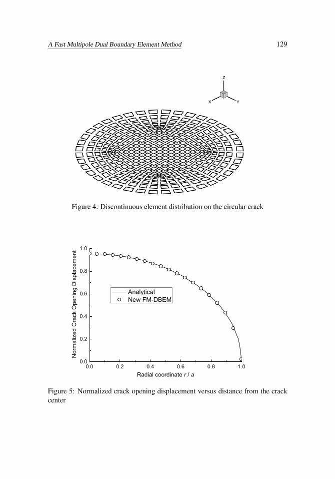
This test involves the analysis of a circular crack with radius a in an infinite solidunder a tensile load σ perpendicular to the crack. The crack is discretized into300 discontinuous elements with 7,200 DOFs as shown in Fig. 4 (each element isplotted as four corner collocation nodes connected with solid lines in order onlyto show the effect of discontinuity). The crack opening displacement ∆un is eval-uated using the new fast multipole DBEM. We take 18 terms for the multipole,local and exponential expansions. The calculated normalized crack opening dis-placement G∆un/(aσ) along the radial direction of the crack is plotted in Fig. 5and compared with the analytical solution. Good agreement is observed, demon-strating high accuracy of the proposed method and capability of the quarter-pointelement for modelling square root behavior of the crack opening displacements atcrack fronts.


X Y

Z

Figure 4: Discontinuous element distribution on the circular crack

Figure 5: Normalized crack opening displacement versus distance from the crackcenter


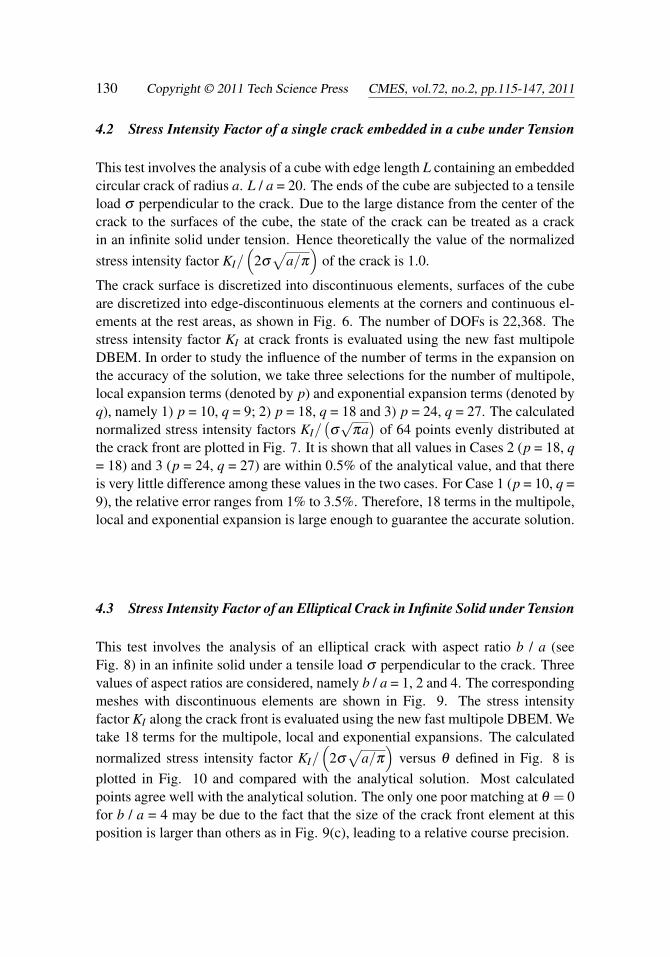
4.2 Stress Intensity Factor of a single crack embedded in a cube under Tension

This test involves the analysis of a cube with edge length L containing an embeddedcircular crack of radius a. L / a = 20. The ends of the cube are subjected to a tensileload σ perpendicular to the crack. Due to the large distance from the center of thecrack to the surfaces of the cube, the state of the crack can be treated as a crackin an infinite solid under tension. Hence theoretically the value of the normalizedstress intensity factor KI/

(2σ√

a/π

)of the crack is 1.0.

The crack surface is discretized into discontinuous elements, surfaces of the cubeare discretized into edge-discontinuous elements at the corners and continuous el-ements at the rest areas, as shown in Fig. 6. The number of DOFs is 22,368. Thestress intensity factor KI at crack fronts is evaluated using the new fast multipoleDBEM. In order to study the influence of the number of terms in the expansion onthe accuracy of the solution, we take three selections for the number of multipole,local expansion terms (denoted by p) and exponential expansion terms (denoted byq), namely 1) p = 10, q = 9; 2) p = 18, q = 18 and 3) p = 24, q = 27. The calculatednormalized stress intensity factors KI/

(σ√

πa)

of 64 points evenly distributed atthe crack front are plotted in Fig. 7. It is shown that all values in Cases 2 (p = 18, q= 18) and 3 (p = 24, q = 27) are within 0.5% of the analytical value, and that thereis very little difference among these values in the two cases. For Case 1 (p = 10, q =9), the relative error ranges from 1% to 3.5%. Therefore, 18 terms in the multipole,local and exponential expansion is large enough to guarantee the accurate solution.

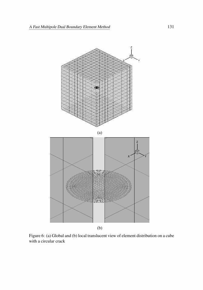
4.3 Stress Intensity Factor of an Elliptical Crack in Infinite Solid under Tension

This test involves the analysis of an elliptical crack with aspect ratio b / a (seeFig. 8) in an infinite solid under a tensile load σ perpendicular to the crack. Threevalues of aspect ratios are considered, namely b / a = 1, 2 and 4. The correspondingmeshes with discontinuous elements are shown in Fig. 9. The stress intensityfactor KI along the crack front is evaluated using the new fast multipole DBEM. Wetake 18 terms for the multipole, local and exponential expansions. The calculatednormalized stress intensity factor KI/

(2σ√

a/π

)versus θ defined in Fig. 8 is

plotted in Fig. 10 and compared with the analytical solution. Most calculatedpoints agree well with the analytical solution. The only one poor matching at θ = 0for b / a = 4 may be due to the fact that the size of the crack front element at thisposition is larger than others as in Fig. 9(c), leading to a relative course precision.


(a)

(b)

Figure 6: (a) Global and (b) local translucent view of element distribution on a cubewith a circular crack


Figure 7: Normalized stress intensity factors KI/(

2σ√

a/π

)of a single crack

embedded in a cube

a

b

è

rK

I

Figure 8: An elliptical crack with aspect ratio b / a


(a)

(b)

(c)

Figure 9: Discontinuous element distribution on the elliptical crack (a) b / a = 1 (b)b / a = 2 (c) b / a = 4

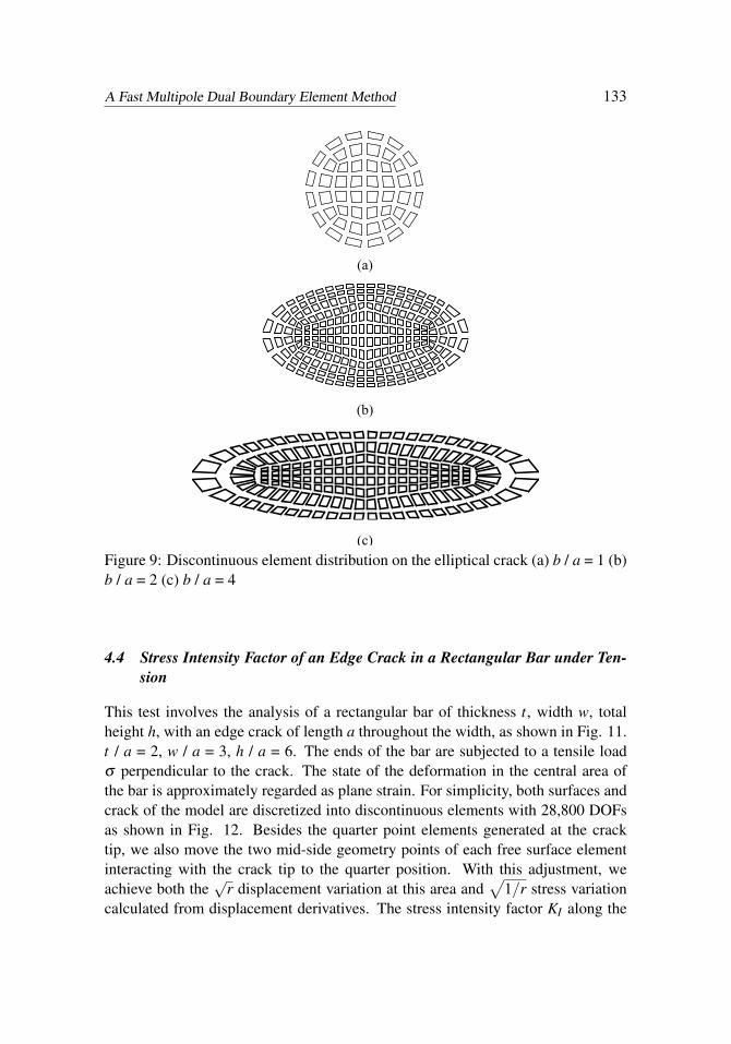
4.4 Stress Intensity Factor of an Edge Crack in a Rectangular Bar under Ten-sion

This test involves the analysis of a rectangular bar of thickness t, width w, totalheight h, with an edge crack of length a throughout the width, as shown in Fig. 11.t / a = 2, w / a = 3, h / a = 6. The ends of the bar are subjected to a tensile loadσ perpendicular to the crack. The state of the deformation in the central area ofthe bar is approximately regarded as plane strain. For simplicity, both surfaces andcrack of the model are discretized into discontinuous elements with 28,800 DOFsas shown in Fig. 12. Besides the quarter point elements generated at the cracktip, we also move the two mid-side geometry points of each free surface elementinteracting with the crack tip to the quarter position. With this adjustment, weachieve both the

√r displacement variation at this area and

√1/r stress variation

calculated from displacement derivatives. The stress intensity factor KI along the


Figure 10: Normalized stress intensity factor KI/(

2σ√

a/π

)versus θ

crack front is evaluated using the new fast multipole DBEM. We take 18 terms forthe multipole, local and exponential expansions. The calculated normalized stressintensity factor KI/

(σ√

πa)

is plotted in Fig. 13 and compared with the analyticalplane strain solution. The numerical result at the center of the bar is within 2% ofthe plane strain value.

Stresses on free surfaces are postprocessed using displacement derivatives. Thecalculated normalized radial stresses σrr (

√a/KI) (see Fig. 11) near the crack tip

(r� a) are 1.24 at r/a = 0.0625,θ = 0 and 1.65 at r/a = 0.0625,θ = π/2, within23% and 3% of the plane stress values 1.59 and 1.69 from Eq. (11), respectively.It is shown that surface stresses calculated from displacement derivatives have rel-atively poor accuracy compared with the stress intensity factor.

σrr =KI

4√

2πr

(5cos

θ

2− cos

32

θ

)⇒ σrr

(√a/KI

)=

14√

2π

√ar

(5cos

θ

2− cos

32

θ

), r� a (11)


ó

ó

a

tt

a

w

h è

rró

Figure 11: A rectangular bar with an edge crack throughout the width

X Y

Z

Figure 12: Discontinuous element distribution on the edge-cracked bar


Figure 13: Normalized stress intensity factor KI/(σ√

πa)

along the crack front

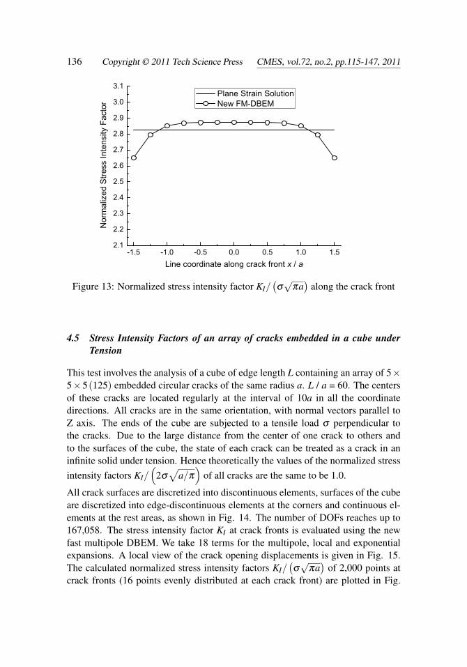
4.5 Stress Intensity Factors of an array of cracks embedded in a cube underTension

This test involves the analysis of a cube of edge length L containing an array of 5×5×5(125) embedded circular cracks of the same radius a. L / a = 60. The centersof these cracks are located regularly at the interval of 10a in all the coordinatedirections. All cracks are in the same orientation, with normal vectors parallel toZ axis. The ends of the cube are subjected to a tensile load σ perpendicular tothe cracks. Due to the large distance from the center of one crack to others andto the surfaces of the cube, the state of each crack can be treated as a crack in aninfinite solid under tension. Hence theoretically the values of the normalized stressintensity factors KI/

(2σ√

a/π

)of all cracks are the same to be 1.0.

All crack surfaces are discretized into discontinuous elements, surfaces of the cubeare discretized into edge-discontinuous elements at the corners and continuous el-ements at the rest areas, as shown in Fig. 14. The number of DOFs reaches up to167,058. The stress intensity factor KI at crack fronts is evaluated using the newfast multipole DBEM. We take 18 terms for the multipole, local and exponentialexpansions. A local view of the crack opening displacements is given in Fig. 15.The calculated normalized stress intensity factors KI/

(σ√

πa)

of 2,000 points atcrack fronts (16 points evenly distributed at each crack front) are plotted in Fig.


16. It is shown that most values are within 1% of the analytical value, and thatthe biggest error is within 1.4%. The results clearly demonstrate accuracy of theproposed method for large-scale problems.

4.6 Memory Requirement and Solution Time of New Fast Multipole DBEM

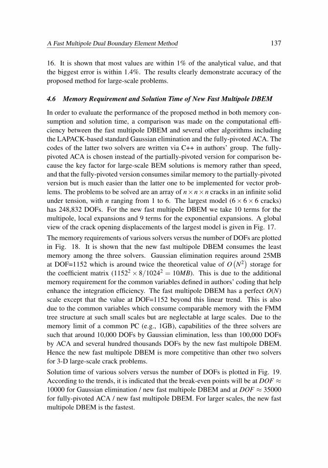
In order to evaluate the performance of the proposed method in both memory con-sumption and solution time, a comparison was made on the computational effi-ciency between the fast multipole DBEM and several other algorithms includingthe LAPACK-based standard Gaussian elimination and the fully-pivoted ACA. Thecodes of the latter two solvers are written via C++ in authors’ group. The fully-pivoted ACA is chosen instead of the partially-pivoted version for comparison be-cause the key factor for large-scale BEM solutions is memory rather than speed,and that the fully-pivoted version consumes similar memory to the partially-pivotedversion but is much easier than the latter one to be implemented for vector prob-lems. The problems to be solved are an array of n×n×n cracks in an infinite solidunder tension, with n ranging from 1 to 6. The largest model (6× 6× 6 cracks)has 248,832 DOFs. For the new fast multipole DBEM we take 10 terms for themultipole, local expansions and 9 terms for the exponential expansions. A globalview of the crack opening displacements of the largest model is given in Fig. 17.

The memory requirements of various solvers versus the number of DOFs are plottedin Fig. 18. It is shown that the new fast multipole DBEM consumes the leastmemory among the three solvers. Gaussian elimination requires around 25MBat DOF=1152 which is around twice the theoretical value of O

(N2)

storage forthe coefficient matrix (11522× 8/10242 = 10MB). This is due to the additionalmemory requirement for the common variables defined in authors’ coding that helpenhance the integration efficiency. The fast multipole DBEM has a perfect O(N)scale except that the value at DOF=1152 beyond this linear trend. This is alsodue to the common variables which consume comparable memory with the FMMtree structure at such small scales but are neglectable at large scales. Due to thememory limit of a common PC (e.g., 1GB), capabilities of the three solvers aresuch that around 10,000 DOFs by Gaussian elimination, less than 100,000 DOFsby ACA and several hundred thousands DOFs by the new fast multipole DBEM.Hence the new fast multipole DBEM is more competitive than other two solversfor 3-D large-scale crack problems.

Solution time of various solvers versus the number of DOFs is plotted in Fig. 19.According to the trends, it is indicated that the break-even points will be at DOF ≈10000 for Gaussian elimination / new fast multipole DBEM and at DOF ≈ 35000for fully-pivoted ACA / new fast multipole DBEM. For larger scales, the new fastmultipole DBEM is the fastest.


(a)

X Y

Z

(b)

Figure 14: (a) Global translucent view and (b) local view of element distributionon a cube containing an array of 5×5×5(= 125) circular cracks


Figure 15: Local view of crack opening displacements

Figure 16: Normalized stress intensity factors KI/(

2σ√

a/π

)of 5×5×5(= 125)

circular cracks


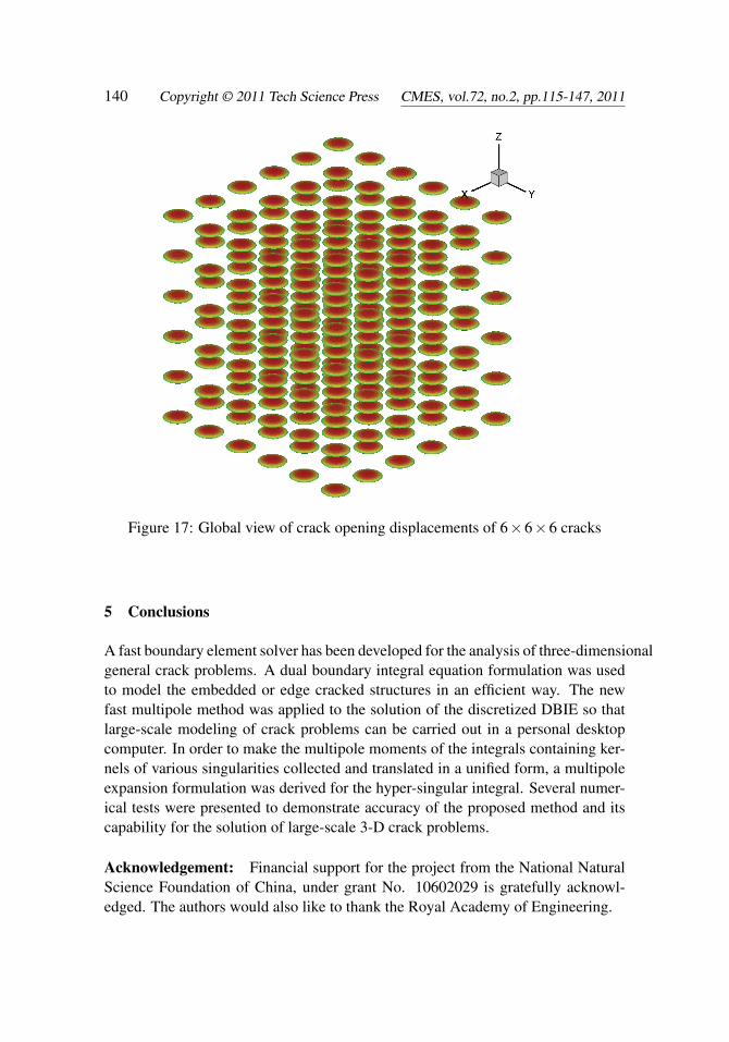
Figure 17: Global view of crack opening displacements of 6×6×6 cracks

5 Conclusions

A fast boundary element solver has been developed for the analysis of three-dimensionalgeneral crack problems. A dual boundary integral equation formulation was usedto model the embedded or edge cracked structures in an efficient way. The newfast multipole method was applied to the solution of the discretized DBIE so thatlarge-scale modeling of crack problems can be carried out in a personal desktopcomputer. In order to make the multipole moments of the integrals containing ker-nels of various singularities collected and translated in a unified form, a multipoleexpansion formulation was derived for the hyper-singular integral. Several numer-ical tests were presented to demonstrate accuracy of the proposed method and itscapability for the solution of large-scale 3-D crack problems.

Acknowledgement: Financial support for the project from the National NaturalScience Foundation of China, under grant No. 10602029 is gratefully acknowl-edged. The authors would also like to thank the Royal Academy of Engineering.


Figure 18: Memory requirement versus DOFs

Figure 19: Solution time versus DOFs


Appendix

In this section, we give a summary of detailed expressions of the multipole mo-ments in Eq. (6). The solid spherical harmonic function and their derivatives aredefined accordingly, which can be found in Yoshida (2001).

Multipole moments:

MU1j,n,m (O) =

∫S0

Rn,m

(−→Oy)

t j (y)dS (y) (A1)

MU2n,m (O) =

∫S0

(−→Oy)

jRn,m

(−→Oy)

t j (y)dS (y) (A2)

MT 1j,n,m (O) =λ

∫S0

∂Rn,m

(−→Oy)

∂y jnk (y)uk (y)dS (y)

+G∫

S0

∂Rn,m

(−→Oy)

∂ykn j (y)uk (y)dS (y)

+G∫

S0

∂Rn,m

(−→Oy)

∂yknk (y)u j (y)dS (y)

(A3)

MT 2n,m (O) =

(3λ +2G)∫

S0

Rn,m

(−→Oy)

nk (y)uk (y)dS (y)

+λ

∫S0

(−→Oy)

j

∂Rn,m

(−→Oy)

∂y jnk (y)uk (y)dS (y)

+G∫

S0

(−→Oy)

j

∂Rn,m

(−→Oy)

∂yk+(−→

Oy)

k

∂Rn,m

(−→Oy)

∂y j

n j (y)uk (y)dS (y)

(A4)

MT 1,Scj,n,m (O) =λ

∫S+

c

∂Rn,m

(−→Oy)

∂y jnk (y)∆uk (y)dS (y)

+G∫

S+c

∂Rn,m

(−→Oy)

∂ykn j (y)∆uk (y)dS (y)

+G∫

S+c

∂Rn,m

(−→Oy)

∂yknk (y)∆u j (y)dS (y)

(A5)


MT 2,Scn,m (O) =

(3λ +2G)∫

S+c

Rn,m

(−→Oy)

nk (y)∆uk (y)dS (y)

+λ

∫S+

c

(−→Oy)

j

∂Rn,m

(−→Oy)

∂y jnk (y)∆uk (y)dS (y)

+G∫

S+c

(−→Oy)

j

∂Rn,m

(−→Oy)

∂yk+(−→

Oy)

k

∂Rn,m

(−→Oy)

∂y j

n j (y)∆uk (y)dS (y)

(A6)

Solid spherical harmonic functions and derivatives:

Rn,m

(−→Oy)

=1

(n+m)!Pm

n (cosθ)eimφ rn (A7)

Sn,m

(−→Oy)

= (n−m)!Pmn (cosθ)eimφ 1

rn+1 (A8)

{r,θ ,φ} are the spherical coordinates of vector−→Oy, Pm

n is the associated Legendrefunction.

∂

∂y1Rn,m

(−→Oy)

=12

[Rn−1,m−1

(−→Oy)−Rn−1,m+1

(−→Oy)]

∂

∂y2Rn,m

(−→Oy)

=i2

[Rn−1,m−1

(−→Oy)

+Rn−1,m+1

(−→Oy)]

∂

∂y3Rn,m

(−→Oy)

= Rn−1,m

(−→Oy) (A9)

∂

∂y1Sn,m

(−→Oy)

=12

[Sn+1,m−1

(−→Oy)−Sn+1,m+1

(−→Oy)]

∂

∂y2Sn,m

(−→Oy)

=i2

[Sn+1,m−1

(−→Oy)

+Sn+1,m+1

(−→Oy)]

∂

∂y3Sn,m

(−→Oy)

=−Sn+1,m

(−→Oy) (A10)

References

Albuquerque, E. L.; Sollero, P.; Aliabadi, M. H. (2004): Dual boundary elementmethod for anisotropic dynamic fracture mechanics. Int J Numer Methods Engng,vol. 59, pp. 1187–1205.

Aliabadi, M. H. (1997): A new generation of boundary element methods in frac-ture mechanics. Int J Fracture, vol. 86, pp. 91–125.


Bebendorf, M.; Rjasanow, S. (2003): Adaptive low-rank approximation of collo-cation matrices. Computing, vol. 70, pp. 1–24.

Benedetti, I.; Aliabadi, M. H.; Davì, G. (2008): A fast 3D dual boundary elementmethod based on hierarchical matrices. Int J Solids and Structures, vol. 45, pp.2355–2376.

Benedetti, I.; Milazzo, A.; Aliabadi, M. H. (2009): A fast dual boundary elementmethod for 3D anisotropic crack problems. Int J Numer Methods Engng, vol. 80,pp. 1356–1378.

Benedetti, I.; Aliabadi, M. H. (2010): A fast hierarchical dual boundary elementmethod for three-dimensional elastodynamic crack problems. Int J Numer MethodsEngng, vol. 84, pp. 1038–1067.

Blandford, G. E.; Ingraffea, A. R.; Liggett, J. A. (1981): Two-dimensional stressintensity factor computations using the boundary element method. Int J NumerMethods Engng, vol. 17, no. 3, pp. 387–404.

Brancati, A.; Aliabadi, M. H.; Benedetti, I. (2009): Hierarchical adaptive crossapproximation GMRES technique for solution of acoustic problems using the bound-ary element method. CMES: Computer Modeling & Engineering Sciences, vol. 43,pp. 149–172.

Brunner, D.; Junge, M.; Rapp, P.; Bebendorf, M.; Gaul, L. (2010): Comparisonof the fast multipole method with hierarchical matrices for the Helmholtz-BEM.CMES: Computer Modeling & Engineering Sciences, vol. 58, pp. 131–158.

Buchau, A.; Rucker, W.; Rain, O.; Rischmüller, V.; Kurz, S.; Rjasanow, S.(2003): Comparison between different approaches for fast and efficient 3-D BEMcomputations. IEEE T Magn, vol. 39, pp. 1107–1110.

Burczynski, T.; Beluch, W. (2001): The identification of cracks using boundaryelements and evolutionary algorithms. Engrg Anal Boundary Elements, vol. 25,pp. 313–322.

Chao, R. M.; Chen, Y. J.; Lin, F. C. (2001): Determining the unknown traction ofa cracked elastic body using the inverse technique with the dual boundary elementmethod. CMES: Computer Modeling in Engineering & Sciences, vol. 2, no. 1, pp.73–85.

Chen, J. T.; Chen, K. H.; Yeih, W.; Shieh, N. C. (1998): Dual boundary elementanalysis for cracked bars under torsion. Engineering Computations, vol.15, no.6-7, pp. 732–749.

Chen, W. H.; Chen, T. C. (1995): An efficient dual boundary-element techniquefor a 2-dimensional fracture problem with multiple cracks. Int J Numer MethodsEngng, vol. 38, no. 10, pp. 1739–1756.


Cisilino, A. P.; Aliabadi, M. H. (1997): Three-dimensional BEM analysis forfatigue crack growth in welded components. Int J Pres Ves & Piping, vol. 70, pp.135–144.

Cisilino, A. P.; Aliabadi, M. H. (2004): Dual boundary element assessment ofthree-dimensional fatigue crack growth. Engrg Anal Boundary Elements, vol. 28,no. 9, pp. 1157–1173.

Cruse, T. A. (1996): BIE fracture mechanics analysis: 25 years of developments.Comput Mech, vol. 18, no. 1, pp. 1–11.

Englund, J. (2006): Efficient algorithm for edge cracked geometries. Int J NumerMethods Engng, vol. 66, pp. 1791–1816.

Fu, Y. H.; Klimkowski, K. J.; Rodin, G. J.; Berger, E.; Browne, J. C.; Singer,J. K.; Geijn, R. A.; Vernaganti, K. S. (1998): A fast solution method for three-dimensional many-particle problems of linear elasticity. Int J Numer Methods En-gng, vol. 42, pp. 1215–1229.

Greengard, L.; Rokhlin, V. (1997): A new version of the fast multipole methodfor the Laplace equation in three dimensions. Acta Numer., vol. 6, pp. 229–270.

Helsing, J. (1999): Fast and accurate numerical solution to an elastostatic probleminvolving ten thousand randomly oriented cracks. Int J Fracture, vol. 100, no. 4,pp. 321–327.

Helsing, J.; Jonsson, A. (2002): Stress calculations on multiply connected do-mains. J Comput Phys, vol. 176, pp. 456–482.

Kebir, H.; Roelandt, J. M.; Chambon, L. (2006): Dual boundary element methodmodelling of aircraft structural joints with multiple site damage. Engng FractureMech, vol. 73, no. 4, pp. 418–434.

Kolk, K.; Weber, W.; Kuhn, G. (2005): Investigation of 3D crack propagationproblems via fast BEM formulations. Comput Mech, vol. 37, pp. 32–40.

Kolk, K.; Kuhn, G. (2006): The advanced simulation of fatigue crack growth incomplex 3D structures. Archive of Applied Mechanics, vol. 76, no. 11-12, 699–709.

Lai, Y. S.; Rodin, G. J. (2003): Fast boundary element method for three-dimensionalsolids containing many cracks. Engrg Anal Boundary Elements, vol. 27, pp. 845–852.

Liu, Y. J.; Nishimura, N.; Otani, Y.; Takahashi, T.; Chen, X. L.; Munakata,H. (2005): A fast boundary element method for the analysis of fiber-reinforcedcomposites based on a rigid-inclusion model. J Appl Mech, vol. 72, no. 1, pp.115–128.

Liu, Y. J. (2006): A new fast multipole boundary element method for solving large-


scale two-dimensional elastostatic problems. Int J Numer Methods Engng, vol. 65,no. 6, pp. 863–881.

Liu, Y. J. (2008): A fast multipole boundary element method for 2D multi-domainelastostatic problems based on a dual BIE formulation, Comp Mech, vol. 42, no. 5,pp. 761–773.

Mi, Y.; Aliabadi, M. H. (1992): Dual boundary element method for three-dimensionalfracture mechanics analysis. Engrg Anal Boundary Elements, vol. 10, pp. 161–171.

Mi, Y.; Aliabadi, M. H. (1994): Three-dimensional crack growth simulation usingBEM. Comput Struct, vol. 52, no. 5, pp. 871–878.

Nishimura, N.; Yoshida, K.; Kobayashi, S. (1999): A fast multipole boundary in-tegral equation method for crack problems in 3D. Engrg Anal Boundary Elements,vol. 23, pp. 97–105.

Nishimura, N. (2002): Fast multipole accelerated boundary integral equation meth-ods. Appl Mech Rev, vol. 55, no. 4, pp. 299–324.

Partheymüller, P.; Haas, M.; Kuhn, G. (2000): Comparison of the basic and thediscontinuity formulation of the 3D-dual boundary element method. Engrg AnalBoundary Elements, vol. 24, pp. 777–788.

Popov, V.; Power, H. (2001): An O(N) Taylor series multipole boundary elementmethod for three-dimensional elasticity problems. Engrg Anal Boundary Elements,vol. 25, pp. 7–18.

Portela, A.; Aliabadi, M. H.; Rooke, D. P. (1992): The dual boundary elementmethod: effective implementation for crack problems. Int J Numer Methods Engng,vol. 33, pp. 1269–1287.

Portela, A.; Aliabadi, M. H.; Rooke, D. P. (1993): Dual boundary element incre-mental analysis of crack propagation. Comput Struct, vol. 46, no. 2, pp. 237–247.

Purbolaksono, I.; Aliabadi, M. H. (2005): Dual boundary element method forinstability analysis of cracked plates. CMES: Computer Modeling in Engineering& Sciences, vol. 8, no. 1, pp. 73–90.

Rokhlin, V. (1985): Rapid solution of integral equations of classical potential the-ory. J Comp Phys, vol. 60, pp. 187–207.

Salgado, N. K.; Aliabadi, M. H. (1996): The application of the dual boundaryelement method to the analysis of cracked stiffened panels. Engng Fracture Mech,vol. 54, no. 1, pp. 91–105.

Sanz, J. A.; Bonnet, M.; Dominguez, J. (2008): Fast multipole method applied to3-D frequency domain elastodynamics. Engrg Anal Boundary Elements, vol. 32,pp. 787–795.


Snyder, M. D.; Cruse, T. A. (1975): Boundary-integral equation analysis of crackedanisotropic plates. Int J Fracture, vol. 11, pp. 315–328.

Takahashi, T.; Nishimura, N.; Kobayashi, S. (2003): A fast BIEM for three-dimensional elastodynamics in time domain. Engrg Anal Boundary Elements, vol.27, pp. 803–823.

Wang, H. T.; Yao, Z. H. (2005): A new fast multipole boundary element methodfor large scale analysis of mechanical properties in 3-D particle-reinforced com-posites. CMES: Computer Modeling in Engineering & Science, vol. 7, no. 1, pp.85–95.

Wang, H. T.; Hall, G.; Yu, S. Y.; Yao, Z. H. (2008): Numerical simulation ofgraphite properties using X-ray tomography and fast multipole boundary elementmethod. CMES: Computer Modeling in Engineering & Sciences, vol. 37, no. 2,pp. 153–174.

Wang, H. T.; Yao, Z. H. (2008): A rigid-fiber-based boundary element model forstrength simulation of carbon nanotube reinforced composites. CMES: ComputerModeling in Engineering & Sciences, vol. 29, no. 1, pp. 1–13.

Wang, P. B.; Yao, Z. H. (2006): Fast multipole DBEM analysis of fatigue crackgrowth. Comput Mech, vol. 38, no. 3, pp. 223–233.

Weaver, J. (1977): Three-dimensional crack analysis. Int J Solids and Structures,vol. 13, no. 4, pp. 321–330.

Weber, W.; Kolk, K.; Kuhn, G. (2009): Acceleration of 3D crack propagationsimulation by the utilization of fast BEM-techniques. Engrg Anal Boundary Ele-ments, vol. 33, no. 8-9, pp. 1005–1015.

Wilde, A. J.; Aliabadi, M. H. (1999): A 3-D dual BEM formulation for the anal-ysis of crack growth. Comput Mech, vol. 23, pp. 250–257.

Yoshida, K.; Nishimura, N.; Kobayashi, S. (2001): Application of fast multipoleGalerkin boundary integral equation method to elastostatic crack problems in 3D.Int J Numer Methods Engng, vol. 50, pp. 525–547.

Yoshida, K. (2001): Applications of fast multipole method to boundary integralequation method. Ph.D. dissertation, Department of Global Environment Engi-neering, Kyoto University.

Young, A. (1996): A single-domain boundary element method for 3-D elastostaticcrack analysis using continuous elements. Int J Numer Methods Engng, vol. 39,pp. 1265–1293.

a fast multipole dual boundary element method for the … · a fast multipole dual boundary element...

Documents