
Enhancing Wireless Sensor Networks Functionalities
by
Davood Izadi
Bachelor of Engineering (Electronic)
Master of Engineering (Electronic and Telecommunication)
Submitted in fulfilment of the requirements for the degree of
Doctor of Philosophy
Deakin University
Jul 2014


iv
Acknowledgement
Foremost, I would like to express my sincere gratitude to my supervisor Prof. Jemal
Abawajy for the continuous support of my Ph.D study and research, his patience,
motivation, enthusiasm and immense knowledge. His guidance helped me in all the time of
research and writing of this thesis. The experience working under his supervision has
redefined many aims in my life.
Thank you to my father and mother that I receive my deepest gratitude and love from their
dedication during my studies.
Thank you to my brothers, who are always supportive.
I would like to thank my wife, for her understanding and love during the past few years.
Her support and encouragement was in the end what made this dissertation possible. Thank you to our research group members Izuan, Ammar, Zulkifli, Meslina, Mesitah, Isredza, and
others. I’ll be remembering our group meeting and lunch fondly.
Davood Izadi
14 November 2014
Melbourne, Australia

v
List of Publication
2014:
Davood Izadi, Jemal Abawajy and Sara Ghanavati (2014), Fuzzy Logic Optimized Wireless Sensor Network Clustering Protocol, Kes journal, IOS Press, Netherlands ISSN: 1327-2314 “Accepted on May 2014”
Davood Izadi, Jemal Abawajy and Sara Ghanavati (2014), A Data Fusion Method in WSNs, Journal of sensors (ISSN: 1424-8220). “Accepted on OCT 2014”
Davood Izadi, Jemal Abawajy and Sara Ghanavati (2014), An alternative node deployment scheme in WSN. IEEE Sensors Journal (ISSN: 1530-437X), DOI: 10.1109/JSEN.2014.2351405. “Accepted on Aug 2014”
Davood Izadi and Abawajy, Jemal and Ghanavati, Sara (2014), An Alternative Data Collection Scheduling Scheme for Enhancing Energy Consumption in Wireless Sensor Networks, Journal of sensors (ISSN: 1424-8220). “Accepted on Nov 2014”
Izadi, Davood, Abawajy, Jemal and Ghanavati, Sara (2014), An Energy Efficient Self-Configurable Clustering Scheme in WSN, IEEE Sensors Journal (ISSN: 1530-437X). “Under review”
2013:
Izadi, Davood, Abawajy, Jemal and Ghanavati, Sara (2013) Fuzzy logic optimized wireless sensor network routing protocol, Journal of high speed networks, vol. 19, no. 2, pp. 115-128, IOS Press, Amsterdam, The Netherlands.
Sarah Ghanavati, Jemal Abawajy and Davood Izadi (2013), A Fuzzy Technique to Control Congestion in WSN, Proceedings of the International Joint Conference on Neural Networks, 4-9 August 2013, Dallas, Texas, USA. “Accepted”
Izadi, Davood, Abawajy, Jemal and Ghanavati, Sarah. (2013), A self-configurable CH selection Scheme in WSN, 14th Proceeding of the Information Reuse and Integration Conference (IEEE IRI), 2013, San Francisco, USA. “Accepted”
2012:
Izadi, Davood, Abawajy, Jemal and Ghanavati, Sarah. (2012) Quality control of sensor network data, in Lee, Gary (eds), Advances in automation and robotics, vol.1, selected papers from the 2011 International Conference on Automation and Robotics (ICAR 2011), Dubai, December 1-2, 2011, pp. 467-480, Springer, Berlin, Germany. “Published”

vi
Abstract
WSNs facilitate the detection of numerous real world phenomena such as natural disaster
and structural faults. The networks collect information from a particular area and transfer it
to a centre for further process. In the data collecting process, there are many considerable
issues that might influence quality of service (QoS). Therefore, it is always necessary to be
considered about the unpredicted events that might negatively influence QoS in WSNs. The
main objective of this research is firstly, to identify the existing gaps in providing a better
QoS in the networks. Although many problems can be addressed in this area, only four of
them are studied in this thesis. First, a new clustering method for the sensors nodes is
proposed to ensure the clusters’ formation are maintained during the network lifetime. Next,
a concept of quality based data fusion mechanism that deals with collecting and sending
only valued data is introduced. In the proposed approach, the nodes play an important role
in distinguishing and transferring only valued data. The valued data will then be aggregated
and transferred to a base station. In the process of routing the data packets, QoS might also
be influenced due to issues such as node failure. Therefore, as a contribution of this thesis
we proposed two routing protocols in WSNs that can adjust themselves with changes in
nodes’ conditions and behaviour. First, the base station is similar to the other deployed
sensor nodes is stationary. Each node is responsible to take the current condition of
immediate nodes into consideration in a real time to find the most appropriate next hub.
Next, we extend the protocol by replacing a mobile sink with the stationary base station.
The mobile sink is capable to schedule itself, based on current conditions of the nodes.
Therefore, the mobile sink instead of randomly or in an order visits the sensor nodes, can
visit the source nodes in a priority manner. Finally, the concept of coverage-hole recovery
is introduced to deal with loss of coverage arising from node failure in post deployment
scenario. The proposed approach finds the uncovered areas and then, virtually force the
nodes to move through the areas.

vii
Table of Content
Table of Content……. ........................................................................................................ vii List of Figures............. ........................................................................................................ ix List of Tables.............. ......................................................................................................... xi CHAPTER 1 ......................................................................................................................... 1 Introduction .......................................................................................................................... 1
1.1. Research Motivation .............................................................................................. 2 1.2. Research Problem .................................................................................................. 3 1.3. Methodology .......................................................................................................... 6 1.4. Research Objectives ............................................................................................... 8 1.5. Research Contributions .......................................................................................... 9 1.6. Thesis Organization ............................................................................................. 11
CHAPTER 2 ....................................................................................................................... 13 Literature Review ............................................................................................................... 13
2.1. Introduction.. ........................................................................................................ 13 2.1.1.WSN Applications ......................................................................................... 17 2.1.2.Event Detection in WSN ............................................................................... 19
2.2. Quality of Service (QoS) ...................................................................................... 21 2.3. A Taxonomy of QoS-Based Protocols ................................................................. 23 2.3.1.Self-Configurable Clustering WSN.................................................................... 23 2.3.2.Quality Based Data Fusion Mechanism ............................................................. 28
2.3.2.1Structured Based Fusion Method ................................................................ 29 2.3.2.1.1Cluster-Based Data Fusioin Method .................................................... 29 2.3.2.1.2Tree Based Data Fusion Method ......................................................... 31 2.3.2.1.3Grid-Based Data fusion Method .......................................................... 32
2.3.2.2.Structure Free Based Fusion Method ......................................................... 34 2.3.3.Routing Protocols in WSN ................................................................................. 35
2.3.3.1.Routing Protocols with Stationary BS ........................................................ 36 2.3.3.2.Routing Protocols Using MBS ................................................................... 39
2.3.3.2.1.Backbone Based Structure with Mobile BS ....................................... 41 2.3.3.2.2.Tree Based Structure with Mobile BS ................................................ 43
2.3.4.WSN Coverage Method ..................................................................................... 45 2.4. Chapter Summary ................................................................................................ 48
CHAPTER 3 ....................................................................................................................... 50 A Self-Configurable Clustering Scheme in WSN .............................................................. 50
3.1. Introduction.. ........................................................................................................ 50 3.2. Problem Overview ............................................................................................... 53 3.3. Self-Configurable Clustering ............................................................................... 55 3.4. Performance Analysis .......................................................................................... 60
3.4.1.Experimental Setup ....................................................................................... 61 3.4.2.Result and Discussion.................................................................................... 61
3.5. Chapter Summary ................................................................................................ 66 CHAPTER 4 ....................................................................................................................... 67 A Data Fusion Method in WSN ......................................................................................... 67

viii
4.1. Introduction.. ........................................................................................................ 68 4.2. Research Problem ................................................................................................ 69
4.2.1.Data Quality….. ............................................................................................ 71 4.2.2.Data Redundancy........................................................................................... 72
4.3. Data Fusion Algorithm ......................................................................................... 73 4.4. Application… ....................................................................................................... 77 4.5. Performance Analysis........................................................................................... 78
4.5.1. Experimental Setup ...................................................................................... 78 4.5.2. Result and Discussion................................................................................... 79
4.6. Chapter Summary ................................................................................................. 83 CHAPTER 5 ....................................................................................................................... 84 Routing WSN Data ............................................................................................................ 84
5.1. Introduction… ...................................................................................................... 84 5.2. Problem Description ............................................................................................ 86
5.2.1.Problem Formulation ..................................................................................... 87 5.3. Reactive Routing Algorithm ................................................................................ 88 5.4. Performance Analysis .......................................................................................... 98
5.4.1.Stationary Sensor Nodes and a BS ................................................................ 98 5.4.1.1.Experiment Setup………… ................................................................... 98 5.4.1.2.Result and Discussion…… .................................................................... 99
5.4.2.Stationary Sensor Nodes with a MBS ......................................................... 104 5.4.2.1.Experiment Setup………… ................................................................. 104 5.4.2.2.Result and Discussion…… .................................................................. 105
5.5. Chapter Summary .............................................................................................. 110 CHAPTER 6 ..................................................................................................................... 111 Dynamic WSN Coverage ................................................................................................. 111
6.1. Introduction… .................................................................................................... 111 6.2. Problem Description .......................................................................................... 115
6.2.1.Problem Formulation.. ................................................................................. 117 6.3. Self-Healing Algorithm ...................................................................................... 118 6.4. Performance Analysis ........................................................................................ 122
6.4.1.Experimental Setup… ................................................................................. 123 6.4.2.Result and Discussion.................................................................................. 124
6.5. Chapter Summary .............................................................................................. 128 CHAPTER 7 ..................................................................................................................... 130 Summary and Future Research Directions ....................................................................... 130
A. Conclusion… ..................................................................................................... 130 B. System Implications ........................................................................................... 134 C. Future Directions ................................................................................................ 135
REFERENCES ................................................................................................................. 137

ix
List of Figures Figure 1.1 Schematic view of the overall research contribution ........................................ 11 Figure 2.1. A general view of a WSN ................................................................................ 14 Figure 2.2. Sensor node ...................................................................................................... 15 Figure 2.3. Interval Type 2 FLS ......................................................................................... 21 Figure 2.4. Classification of aggregating data protocols in a WSN ................................... 29 Figure 2.5. Chain based protocol ....................................................................................... 30 Figure 2.6. Tree-based data fusion protocol ....................................................................... 31 Figure 2.7. Data aggregation methods ............................................................................... 33 Figure 3.1. A clustered WSN ............................................................................................. 52 Figure 3.2. Clustering formation of sensor nodes .............................................................. 53 Figure 3.3. A deployed node with neighbours ................................................................... 56 Figure 3.4. Eligibility of each node .................................................................................... 56 Figure 3.5. CH joining message ......................................................................................... 57 Figure 3.6 Allocated TDMAs for (a) CH and (b) CM. ...................................................... 59 Figure 3.7. Radio energy dissipation model ....................................................................... 60 Figure 3.8. Comparison of the response surface generated by the Fuzzy systems ............ 63 Figure 3.9. Energy consumption ........................................................................................ 64 Figure 3.10. Data loss rate .................................................................................................. 64 Figure 3.11. Message Overhead in cluster ......................................................................... 66 Figure 4.1. Fusion mechanism ........................................................................................... 70 Figure 4.2. Proposed flow chart ......................................................................................... 73 Figure 4.3: Proposed FLC .................................................................................................. 73 Figure 4.4. Event probability in FIS ................................................................................... 76 Figure 4.5. Forest fire application ...................................................................................... 78 Figure 4.6. Data collection ................................................................................................. 80 Figure 4.7. Transferred data packets .................................................................................. 81 Figure 4.8. Energy consumption ........................................................................................ 82 Figure 5.1. T shows and compares the distance from A and B .......................................... 90 Figure 5.2. Grid cluster formation Network ....................................................................... 92 Figure 5.3. FLS3 for controlling MBS ............................................................................... 94 Figure 5.4. RTR message ................................................................................................... 95 Figure 5.5. ATR message ................................................................................................... 95 Figure 5.6. TDMA structure ............................................................................................... 96 Figure 5.7. Emergency message ......................................................................................... 96 Figure 5.8. Comparison of the surfaces of the type 1 FLS (a) and the proposed approach(b) .......................................................................................................................................... 100 Figure 5.9. Energy Consumption ..................................................................................... 101 Figure 5.10. Relation of data received and required energy ............................................ 102 Figure 5.11. A comparison of remaining buffer capacity ................................................ 103 Figure 5.12. A comparison of unsuccessful transmissions .............................................. 104 Figure 5.13. Average energy consumption ...................................................................... 106 Figure 5.14. Energy consumption of border nodes .......................................................... 107 Figure 5.15. End-to-end delay .......................................................................................... 108 Figure 5.16. Unsuccessful transmission ........................................................................... 109 Figure 6.1. Over lapping with uncovered area ............................................................... 1166

x
Figure 6.2. Coverage-hole ................................................................................................ 117 Figure 6.3. A failed node in a WSN ................................................................................. 119 Figure 6.4. Coverage Enhancement ................................................................................. 120 Figure 6.5. Relocation message ........................................................................................ 122 Figure 6.6. Random deployment ...................................................................................... 124 Figure 6.7. Average energy consumption ........................................................................ 125 Figure 6.8. Coverage ........................................................................................................ 126 Figure 6.9. Coverage ratio ................................................................................................ 127 Figure 6.10. Uniformity ................................................................................................... 128

xi
List of Tables Table 2.1. The comparison of different clustering protocols with respect of QoS ............ 27 Table 2.2. Comparison of routing protocols for WSN ....................................................... 39 Table 2.3.The comparison of different routing protocols using MBS with respect of QoS ............................................................................................................................................ 44 Table 2.4. The comparison of different coverage protocols with respect of QoS .............. 48 Table 4.1. Parameters of MTS420/400 .............................................................................. 79 Table 5.1. Notations ........................................................................................................... 86 Table.6.1 Notations .......................................................................................................... 117

1
Chapter 1
INTRODUCTION
Advances in micro electro mechanical systems (MEMS) technology has provided the
opportunity for developing tiny and low-cost sensor nodes containing on-board sensing,
signal processing and wireless communication capabilities. These sensor nodes are capable
of converting environmental phenomenon into digital signals and send them to other nodes.
Each individual node has limited capabilities that might not be able to use in different
monitoring systems. However, a combination of hundreds or thousands of them can
coordinate by forming wireless sensor networks (WSNs). A WSN is a compact sensing
system with a collection of wireless sensor nodes deployed on a region of interest with the
purpose of sensing events in a collaborating manner. WSN can be used in many real world
applications. Some of these applications require a very high level of performance, reliability
and accuracy. Therefore, it is always necessary to consider quality of service (QoS) in
WSNs. QoS based on the requirements of WSNs can be used in different meaning and
prospective. Nevertheless, QoS in any WSNs is used to enhance the performance of WSNs

2
for users [1]. In this thesis QoS is analysed based on the consideration of different
requirements such as energy consumption, delay, traffic overhead and successful
transmission. To enhance them, there are many research questions can be addressed. In this
chapter, four research questions with the motivations behind them are introduced.
1.1. Research Motivation
In WSNs QoS can be affected by different reasons. First, the WSN deployment
method is one of the most important factors that can influence the data quality. Unreliable
or even not suitable model for a WSN can make the sensor nodes waste their limited power
and loss data as well as increasing overhead traffic in the network. Another reason that
influences QoS is the data fusion mechanism used. Unreliable data fusion mechanisms
might increase traffic overhead as well as unsuccessful data transmissions in WSNs.
Therefore, as a result of resubmission process, energy consumption would be increased in
such networks. Next, a comprehensive routing protocol can play a significant role in
transferring higher quality data packets to base station (BS). Each routing protocol needs to
be highly capable of adopting itself to different situations. It is also necessary for a source
node with important data to make sure that BS can receive the data on time. Failure in
receiving data by BS increases the requirement of data packet re-transmissions. Therefore,
the QoS requirements such as delay, traffic overhead and energy consumption in the
network will be influenced. Finally, coverage of the network is also one of the most
significant factors that can help to enhance QoS in a WSN data. To make sure that the entire
events in an area of interest are detected and also redundancy in reporting the events is
minimised, it is necessary to develop an optimised coverage method for WSNs.

3
1.2. Research Problem
This thesis deals with QoS requirements such as energy consumption and delay in
WSNs. In particular, we address the following four research questions in this thesis.
How to cluster a WSN to achieve the optimum QoS in the presence of node
failure?
When the entire deployed nodes are required to forward sensed data packets
to the sink, the available energy in each node can be wasted through idle
listening and retransmitting due to collision as well as overhearing. To
overcome that, sensor nodes are clustered for the purpose of energy
minimization. Then, they will be required to communicate with their CHs
instead of sending the data packets directly to BS. However, in the case of
CHs failure, the clustered structure of the network is ruined and consequently
the nodes will be required to be re-clustered again. That causes a lot of
missing data as in cluster creation process, the sensor nodes cannot collect
data.
There are several research work related to cluster formation in WSN [2-4].
Most of them considered various parameters on different conditions to select
the most appropriate CHs in WSN. However, they did not consider CHs
failure, as they can simply be destroyed due to hardware or even software
failures. To address this problem, we propose a cluster formation with
primary and backup CH (BCH). That is to make sure in case of the primary
CHs failure, the BCHs are able to take the responsibility on an appropriate
time. As a result, the sensor nodes can be sure that, even if their CHs are

4
failed, their cluster formation is still active without requiring a new
clustering creation process. In fact, the nodes can keep collecting and
sending their data to BS via their pre-determined backup CHs.
How to aggregate WSN data with maximum QoS assurance?
Data generated from neighbouring sensors is often redundant and
consequently influencing QoS in WSNs [5]. In addition, the amount of data
generated in large sensor networks is usually enormous for BS to process.
Hence, a method to combine data at the sensors or intermediate nodes is
certainly required. Such a method combines different data packets from
different sources without losing important information, while it eliminates
redundant data.
Recently many approaches have been investigated on developing fusion
methods with the purpose of enhancing quality of WSN data [6-8]. However,
the proposed approaches, did not consider specific limitations for sensors’
storages as they can influence QoS in WSN. They simply aggregate the
entire received data from sources that include valued and corrupted data. As
a result, apart from the created a high traffic overflow, energy consumption
in such networks is obviously not efficient.
To address this problem, we propose a data aggregation protocol for WSNs
that can distinguish valued and corrupted data from each other. Then, it
disregards the corrupted data in the fusion process. The proposed protocol
reduces data redundancy as well as enhancing the efficiency of energy
consumption in the WSN.
How to collect data from the WSN in the present of sensor node failure?

5
Node failures that cause loss of connectivity is the most common problem in
dynamic WSNs that causes the collected data are not received by BS. To
overcome the problem, an efficient quality based routing protocol is required
with the capability of adjusting to different unexpected node failure in
WSNs.
During the past decade, considerable research efforts have been investigated
in developing routing techniques in WSNs with stationary and mobile BS
(MBS). Majority of the approaches considered constrains such as energy
efficiency and delay as the main objectives to enhance QoS in the networks.
However, existed developed protocols have limitations in dynamic
environments which contain a variant amount of noise created by
interferences. Additionally, MBS is not capable to schedule itself
intelligently to visit source nodes in an efficient manner. Moreover, MBS in
the existing approaches cannot be called by the source nodes of WSNs. In
fact, it needs to visit the entire source nodes even they are not required to be
visited.
In this thesis, we develop a dynamic data routing approach for WSNs with
the purpose of providing a higher QoS. In that we consider local information
includes noisy data. The MBS used in the approach instead of visiting the
entire source nodes, is able to smartly schedule itself in the most efficient
manner. As a result, we enhance the energy efficiency of the network as well
as reducing the traffic overflow in the WSN.
How to enhance coverage of WSN to improve QoS in the presence of node
failure and coverage redundancy?

6
The importance of this problem arises when a WSN needs to be established
in inaccessible areas such as forests or chemically polluted regions. In such
areas sensors are deployed randomly that is reducing the quality of collected
data. That is because of the low possibility of fully covered sensor field,
while the node are not overlapped.
There are several research work related to the deployment of wireless sensor
nodes [9-11]. Most of them considered a single objective such as coverage
ratio. However, the other objectives such as energy consumption
minimization, uniformity and data reliability are also practically considered
in the choice of deployment process.
This thesis develops a dynamic reconfiguration coverage maintenance
scheme for mobile sensor network to meet the specific requirements of the
event detection system. When a loss of coverage occurs due to reasons such
as dead or noisy sensors, the proposed approach ensures the immediate
neighbours to move and replace with the failure node. As a result of locating
the sensor nodes uniformly in the area of interest, the energy consumption
of the network is consumed more efficiently.
1.3. Methodology
There are many techniques includes statistical and Covariance Intersection (CI)
based methods are used to enhance the QoS in WSNs. However, most of them are not
capable to cope with the uncertainty of the data produced by WSN’s. Moreover, the
inflexibility of the methods prevents processing the data realistically [12]. Applying these
methods requires very complex and very much computational effort for having optimal

7
performance [13]. In contrast, flexibility of fuzzy systems provides us with the opportunity
to edit and display given information at any point of the structuring. In addition, the 3D
display and surface gives us a clearer picture of the output of the system. Therefore, we
decided to use fuzzy logic systems as in many previous works the sensors were equipped
with the systems [14-16]. Type-1 fuzzy logic systems (T1FLS) use fixed fuzzy
memberships that cannot directly address variable conditions. Therefore, uncurtain
measured parameters in applied systems would be neglected by T1FLS and the performance
obviously will be negatively influenced. As a result, Type-2 fuzzy membership functions
that use membership degrees which are themselves fuzzy sets were developed. Type-2 fuzzy
sets are very useful when there is a difficulty in determining appropriate membership
function with ambiguity. Type-2 fuzzy sets allow us to handle linguistic uncertainties.
T2FLS technology has been regarded as a way to increase the fuzziness of a relation means
increased ability to handle inexact information in a logically correct manner [17]. The fuzzy
logic toolbox used in this thesis was built in MATLAB. Therefore, although there are many
simulating software such NS3 or OMNET, we used MATLAB to simulate the proposed
solutions. To test and validate the proposed approaches in this thesis, we conduct
experiments. The inputs of the developed approaches we generate synthetic data. We use a
Gaussian distribution with its mean and covariance matrix representing the expected value
and its uncertainty (10% of the value). Then, the values are normalized to fit in the [0, 1] as
the inputs of the fuzzy system. Then, we extract linguistic variables out of the normalized
data. In each experiment, 20% of the data is used for training the fuzzy system to determine
the membership functions and also the rules as well as the required threshold values for
solutions. Then, we used 80% of the data to test the proposed solutions. In those simulations

8
and experiments, various parameters were used to examine and demonstrate the viability of
the proposed solutions compared to the similar baseline solutions.
We validate our experiments using root-mean-square error (RMSE) as used in previous
works [18-20]. RMSE provides a complete picture of the error distribution in an experiment.
It provides not only a performance measure, but also a representation of the error
distribution. In this thesis RMSE is used to measure of the difference between predicted
values and the result of the proposed approaches and also the existing baseline protocols.
RMSE gives us a single measure of predictive power to compare the performance of the
approaches.
1.4. Research Objectives
The aims of this thesis are:
To propose a distributed and dynamic self-configurable approach for clustering
WSNs, in order to minimize the communication overhead and prolong the network
lifetime;
To develop a cluster based data fusion protocol in order to combine information
from various sources to reduce the amount of raw data transmitted over the network.
To develop two distributed dynamic WSN data routing protocol in WSN with a
stationary and a MBS;
To develop a dynamic distributed coverage strategy in which mobile sensor nodes
have the ability of communicating with each other, detect failed nodes or uncovered
areas and organize themselves to move and maximize coverage.
9
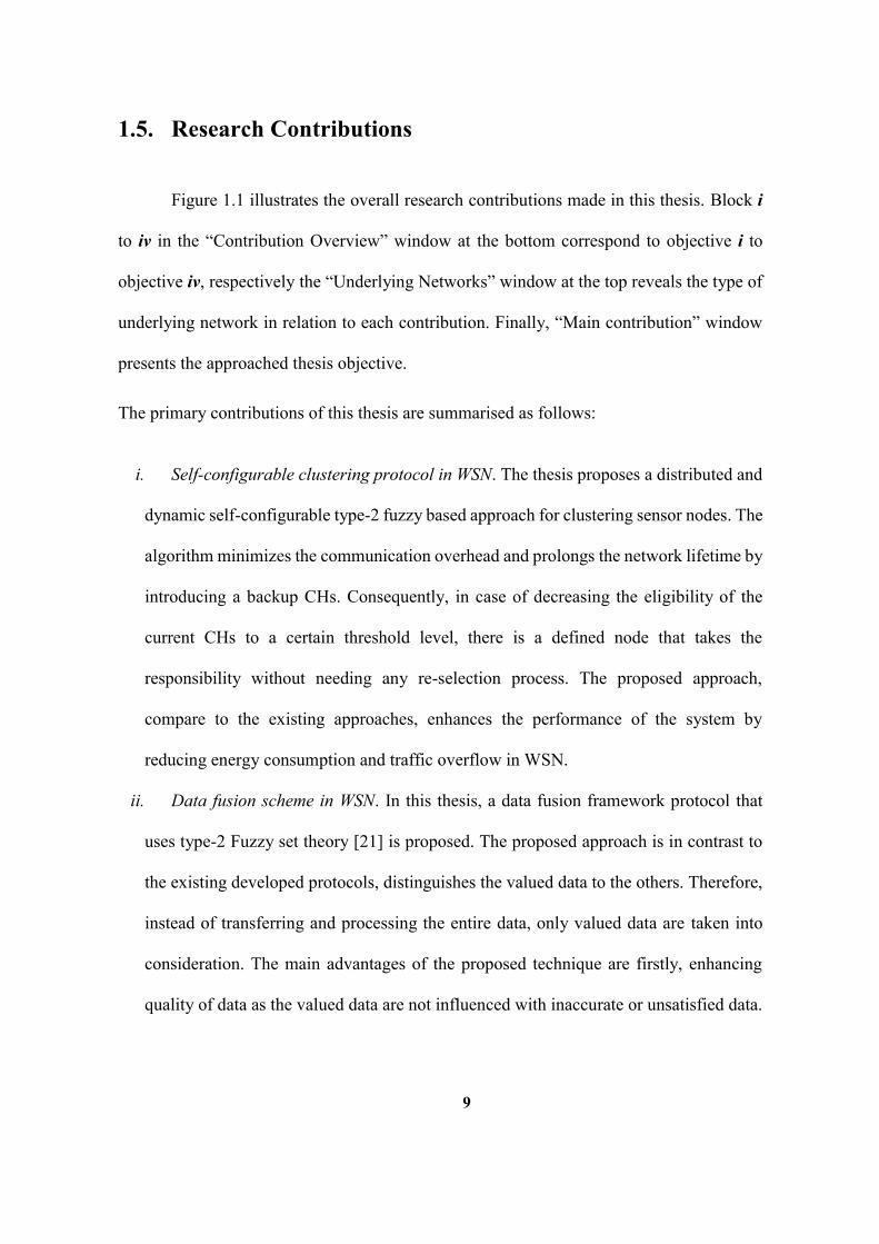
1.5. Research Contributions
Figure 1.1 illustrates the overall research contributions made in this thesis. Block i
to iv in the “Contribution Overview” window at the bottom correspond to objective i to
objective iv, respectively the “Underlying Networks” window at the top reveals the type of
underlying network in relation to each contribution. Finally, “Main contribution” window
presents the approached thesis objective.
The primary contributions of this thesis are summarised as follows:
i. Self-configurable clustering protocol in WSN. The thesis proposes a distributed and
dynamic self-configurable type-2 fuzzy based approach for clustering sensor nodes. The
algorithm minimizes the communication overhead and prolongs the network lifetime by
introducing a backup CHs. Consequently, in case of decreasing the eligibility of the
current CHs to a certain threshold level, there is a defined node that takes the
responsibility without needing any re-selection process. The proposed approach,
compare to the existing approaches, enhances the performance of the system by
reducing energy consumption and traffic overflow in WSN.
ii. Data fusion scheme in WSN. In this thesis, a data fusion framework protocol that
uses type-2 Fuzzy set theory [21] is proposed. The proposed approach is in contrast to
the existing developed protocols, distinguishes the valued data to the others. Therefore,
instead of transferring and processing the entire data, only valued data are taken into
consideration. The main advantages of the proposed technique are firstly, enhancing
quality of data as the valued data are not influenced with inaccurate or unsatisfied data.

10
Next, it enhances the efficiency of energy consumption as the proposed method by
eliminating unvalued data make a reduction in transferring data.
iii. Data routing protocol in WSN. In this thesis, two routing protocols in a WSN with
the purpose of enhancing QoS are proposed. The first proposed approach is basically a
routing protocol with stationary sensor nodes and a BS. Each source node needs to
consider the current condition of neighbours, in real time, through BS to transfer the
data. After that, the proposed protocol is extended by replacing the stationary BS with
a MBS. In the extended version of the approach, we develop a unique flexible visiting
method for MBS. The direction of MBS can be controlled and changes based on sensors’
local information. Additionally, MBS can be called by each node in the sensor field.
iv. A dynamic WSN coverage scheme. In this thesis, a dynamic distributed WSN
coverage maintenance strategy is proposed. In the proposed approach, the mobile sensor
nodes have the ability to communicate with each other, detect failed nodes or uncovered
areas and then, organize themselves to move and maximize coverage. This approach,
unlike the existing approaches does not need to use global information of the network.
QoS is also enhanced as noisy or disordered nodes are detected and then, replaced with
immediate neighbours. Moreover, the energy consumption is become more efficient.
That is due to firstly, less required message exchanges as well as eliminating the noisy
nodes that transfer more bits (noises) in the network. Secondly, the needed energy for
random and inaccurate movement of the mobile nodes is reduced.

11
iiiRouting protocol with guaranteed
QoS
QoS Aware Data Collection in WSN
iClustering
network guarantee QoS
ivDynamic
coverage respect to QoS
iiData fusion Respect to
QoS
Static sensors with mobile sink
Static sensor with fixed sink
Mobile sensor with a fixed sink
Quality control of data
Con
trib
utio
n O
verv
iew
Und
erly
ing
Net
wor
ksM
ain
Con
trib
utio
n
Figure 1.1 Schematic view of the overall research contribution
1.6. Thesis Organization
The remainder of the thesis is organized as the following:
1. Chapter 2: WSN data quality control. This chapter provides an in-depth analysis
and overview of existing WSN data quality control approaches, presented
within a comprehensive taxonomy.

12
2. Chapter 3: WSN clustering. This chapter presents an approach to capable WSN
of self-configurable cluster head (CH) selection and clustering the entire
network.
3. Chapter 4: WSN data fusion. This chapter presents an approach to aggregate
WSN data with considering the current storage condition of sensor nodes.
4. Chapter 5: WSN data routing. In this chapter two routing protocols are
suggested one with stationary BS and other with MBS. In both scenarios, the
network behaviour are analysed separately.
5. Chapter 6. WSN self-configurable coverage scheme. This chapter presents a
protocol that is divided into two phases.
6. Chapter 7. Conclusion and future directions. The concluding chapter provides a
summary of contributions and a future research challenges

13
Chapter 2
LITERATURE REVIEW
This chapter provides a comprehensive review of wireless sensor network (WSN) and
various quality of service (QoS) issues in such networks. It focuses on four of the major
issues which are clustering deployed sensor nodes, data aggregation, proper routing data
packets and converge enhancement with mobile sensors in a WSN. In this chapter, an in-
depth analysis of the existing approaches is presented to identify the addressed research
gaps.
2.1. Introduction
WSN has been an attractive research area and has been used for various applications.
WSN integrates low power communication and consists of a large number of sensor nodes
that communicate with each other. The sensor nodes can be deployed either randomly or
manually depending upon the applications. In addition to the sensor nodes, WSNs need one
or more base stations (BS) to be able to make communications and collect data from the
sensors deployed in the monitored areas. The role of the BS is to maintain the

14
communication between sensor network and external source (users). In fact, the
communications among sensor nodes and the BS provide users with the accessibility of
information from any remote location to allow collecting and analysing the sensor data.
Figure 2. 1. presents a general view of a WSN.
NetworkkNetwork
NNNetwwoooorrrkkkkkNetworkS
Base Station
Figure 2.1. A general view of a WSN
A wireless sensor node is a very small transducer that is capable of convening physical
phenomenon such as sound, light and temperature into electrical signals. The technical
components are consisted of sensor interfaces, circuit, microcontroller, battery and radio
system. Each component and system in the electrical device is required to work properly to
achieve the expected outcome of the device. Figure 2.2 shows a general view of a sensor
node device.

15
RadioBattery
MicrocontrollerCircuit
Sensor Interface
Figure 2.2. Sensor node
In a sensor node the radio subsystem is responsible for data transmission. For this purpose,
each sensor node needs to use radio frequencies to be able to communicate with each other.
In an operating WSN, there are two types of communications, which are infrastructure and
application communication. In infrastructure communication, the sensor nodes are required
to build, maintain and optimize the network. This communication is needed to monitor
environmental changes or node failures. The application communication is required to
forward the collected data to the BS. There are well known technologies such as ZigBee
and IEEE802.11 that manage the radio section of the sensor node. The technologies can
manage the radio data rate, signal frequency and bandwidth [22].
Power subsystem is another technology consideration of the devices. Each sensor node
requires a power unit to function and perform their individual tasks. Power subsystem
provides the supply voltage and the requirements of the power are strict due to energy
constraints. It also supplies sufficient levels of current during radio transmissions and
receptions. In constructing a battery, apart from providing a long life for a WSN, it is
necessary to be aware of the weight, cost and the size of batteries as well as the global
standards for availability and shipping batteries.

16
Microcontroller in a sensor node is usually responsible for adapting the applied routing
methods, efficiently transmitting sensory signals and processing them [23]. This subsystem
also involves data fusion where the different packets arrive from the sensor nodes are
gathered to form a single packet thereby reducing the transmission energy in WSNs. Finally,
circuits and sensor interfaces are responsible for sensing the environment and are controlled
by microcontroller.
After deployment, the sensor nodes are subject to various conditions that have impact on
their performance. Some of these factors include:
Environment factors: Each sensor node for a period of time might be subjected to a non-
operating environmental limitations without permanently changing its performance under
normal operating conditions. Environmental limits are directly related to the storage
conditions of the sensor nodes include the highest and the lowest storage temperatures and
maximum relative humidity at the temperatures. In such conditions the sensors output
signals may increase or decrease which is causing an ultralow frequency noise. Those
changes might be occurring in a short term period of time such as a minute or even in a long
time of sensors’ performance. Therefore, environmental stability, which is a significant
requirement of producing sensor nodes, is necessarily needs to be considered by both sensor
designer and the application engineers.
The most important factor that influences sensors’ performance is their storage temperature.
For sensor nodes, the lower and upper extreme temperature (e.g., -5 C to +80 C) is usually
provided in their data sheets, within which the sensors maintain their specified accuracies.
Sometimes the temperature range might be divided into some sections with their specified
error in nodes’ output. In addition, a relatively fast temperature change may cause the sensor
17
to generate a false output signals. That is because in the case of a quick change, the
temperature, sensors generate an electronic current that might be recognised by their
processing units as a valid response and consequently, cause a false detection [24].
Uncertainty: Sensor nodes manufacturers are aiming to produce the most accurate wireless
sensor nodes to uniformly and consistently collect and process data. However, the reality is
that the produced sensors are never ideal as they carry uncertainty in their measurements.
Therefore, users never can be 100% sure about the created measured values [24]. In fact,
any individual measurement, x, is expected to be presented a bit different to the true
value, That is due to the existed uncertainties that cause errors in the measuring process.
The error is calculated by (2.1).
ɸ = (2.1)
It does not matter how an event (e.g. temperature) is measured by a sensor or how close the
measurement is to the true value, never can it be sure that it is accurate. For example the
uncertainty in measured temperature of a water bath could be up to ɸ = 0.068 [24].
2.1.1. WSN Applications
Applications of WSNs in the event detection domain can be categorised into five
major categories. In this section some of the applications are going to be explored. First,
environment applications in which a large number of sensor nodes are deployed in an area
of interest. They are responsible to detect the environmental phenomenon such as
biodiversity and ecosystem monitoring [25], air pollution monitoring [26], greenhouse
monitoring [27] and food monitoring [28]. Apart from the applications, the use of WSNs in
critical environmental hazard detection and disaster warning system attracted more attention

18
in recent years as it promises safety of human lives and properties. Typical applications in
such forest fire detection [29], volcano monitoring [30] and earthquake warning system [31]
radiation detection [139, 140], chemical and biological hazard detection [32] or any other
meteorological hazard characterised in environments [33]. WSNs can also be applied in
industrial fields for monitoring purposes. The main motivation of using WSNs instead of
the wired sensor networks in industry is the flexibility and the capability of self-
organization. In case of adding or removing a sensor node from the WSN, the networks can
reconfigure itself without being worried about cabling. Moreover, sensor nodes can be place
in a moving part of machineries and inaccessible areas for remote monitoring, where wired
sensors may not be able to apply. WSN are usually used to detect the performance and
operational faults and to detect safety issues in large industrial plants [34], building
automation [35] and structural integrity monitoring [36]. As a result of monitoring and
detecting faults or anomaly in industry possible damages on machineries which could be
very costly could be prevented. Moreover from personal safety point of view, WSNs can
help the operators who work in the industry. Third, WSNs can also be used in emergency
health applications to provide a global and cost effective monitoring system to continuously
and independently monitor a person's physiological conditions. Therefore, in case of any
emergency the corresponding medical centre can be notified. Some of the emergency health
applications include continuous health monitoring and alarm system [37] and fall detection
in elderly care [38]. Finally, WSN can be used in our home applications such as vacuum
cleaners, stoves, stoves and electricity monitoring systems. WSNs can monitor our everyday
life and determine real world phenomena that needs to be taken care of automatically for
smart home system [39, 40].

19
In the all applications, QoS is the main challenging aspect of them that needs to be
considered. To enhance QoS in the applications, deployment methods used for developing
WSNs for the applications is as much important as collecting and aggregating data from the
environments. Transferring data in different environment with different conditions is also
an important key in providing a satisfactory QoS.
2.1.2. Event Detection in WSN
Event detection using WSN technology has been a research area over the past
decades. That is due to the various applications in the real world. Event in WSNs
corresponds to a real world phenomena occurring in environments being monitored. Event
detection process generally can be categorized into two main centralized and distributed
detection classes. In centralized detection based systems, each sensor is required to send its
observations to a centre or a base station without any processing or losing information.
Then, the centre would be in charge to process the received data and realize that whether an
even occurred. That obviously increases the traffic as well as energy consumption since
transferring data consume more energy than processing them. That is clearly become worse
in large scale sensor networks in real world applications with the large amount of
transmissions from sources to the base station [41-43]. That also incurs a significant delay
in event detection process in WSNs. Therefore, decentralized or distributed event detection
scheme can perform better as the sensor nodes are constrained by limited power and
bandwidth communication. In decentralized detection architecture, sensor nodes instead of
sending data packets directly to the base station, they decide on the occurrence of an event,
based on the sensed data. Then, only the decisions are sent to the destination. As a result,
lower consumption of energy and bandwidth in such networks, make the decentralized

20
detection to be the most popular technique in event detection process [42, 44-47]. There are
many proposed techniques and schemes such as patterned based recognition detection
scheme [48-51] and fuzzy logic system [52, 53] that can be used in developing a distributed
architecture. In this research, it is decided to use fuzzy logic system detection.
Krasimira et al. [53] identified fuzzy logic suitable for event detection in WSNs. First, the
system is capable of tolerating unreliable and imprecise sensor readings. Next, the system
work very closely to the natural way of human thinking. Finally, fuzzy logic is much
intuitive compared to other probability theory based methods. In fact, fuzzy logic has
potential to deal with conflicting situations and imprecision in data using heuristic human
reasoning without needing complex mathematical modelling.
There are two types, type 1 and type 2, of fuzzy logic systems. In this thesis only type 2 of
the system is used. The interval T2 (IT2) FLS, which is known as interval-valued, is the
most popular technique that has been using in type-2 fuzzy systems. The basic concept of
IT2-FLS is considering a foot print of uncertainty (FOU), which can be described by two
bounding of T1 fuzzy membership functions [17]. Eq. (2.4) calculates the IT2 fuzzy set .
(2.4)
In this equation, x and u are the primary and the secondary variable and is the primary
membership function of x. In case of IT2 fuzzy sets, all secondary grade of fuzzy set are
equal to 1. The domain of the primary membership defines the FOU of fuzzy set ,
which can be described by its upper and lower membership functions. Hence: FOU ( ) =
.

21
0
0.2
0.4
0
0.6
0.8
1
x
μÃ(x ,u)Ã
μà (x)
μà (x)
FOU(Ã)
Figure 2.3. Interval Type 2 FLS
Figure 2.3 shows a general view of the IT2 with the upper and lower
membership functions. In order to calculate the final output of T2-FLS, there are two
main steps, which are reducing the type 2 to type 1 and then defuzzifing the output. The
first step, type reduction, which is an important calculation for Type-2 FLSs, is a new and
complicated concept. detail of some popular methods in type reduction have been described
in [54]. The second step is defuzzification. In order to obtain a crisp (type-0) output from a
type-2 FLS, the type-reduced set needs to be defuzzified. For this aim, there are many well-
known techniques such as centroid, bisector, mean of maximum, smallest of maximum and
largest of maximum. More details of type reduction methods can be found in [17].
2.2. Quality of Service (QoS)
Different techniques in WSNs may recognize QoS in different ways, which can be
designed based on applications’ requirements. For instance, in a safe control system delay
and packet loss may not be allowed, while it might be acceptable in air conditioning systems
in an office. Nevertheless, QoS methods in any application are applied to enhance
performance of WSNs [55]. There are many considerable challenges that can be categorized
into hardware and software aspects of the networks. This research is more focused on

22
software aspects of the techniques. In this study, the following six parameters are going to
be addressed to enhance QoS in the WSN.
i. Memory Limitation: Since a sensor node is a small device, the memory used in the
device has a strict capacity limitation. Therefore, there is not enough space to run
complicated algorithms and also storing much data. Hence, overflow can be a significant
issue in providing high QoS [56].
ii. Delay: Multi-hop routing, network congestion and data traffics are the reasons behind
delay in wireless communications. That can affect synchronization in the network and
consequently make issues in data collection processing, especially in critical events.
Thus, to ensure data to receive on time to the destination in real time applications, it is
necessary to be aware of delay metrics in developing data collection mechanisms. Notice
that on-time transmission does not mean fast communication or computation but there is
a unique timing requirement for every network that needs to be respected [57].
iii. Power Consumption: Energy consumption is the biggest constraint that needs to be
considered in developing a WSN. In general, energy consumption in a WSN can be
categorized into three main aspects: (i) energy for the sensor transducer, (ii) energy for
communication among sensor nodes and (iii) energy for microprocessor computation. It
has been shown [58] that the required power for transmitting one bit of data in WSNs is
equal to the required energy of processing 800 to 1000 instructions. Consequently,
energy constraint necessarily needs to be taken into account precisely in developing a
routing protocol for a WSN [59].

23
iv. Accuracy: Performance accuracy of WSNs is not only depended on physical properties
of the environment. Developed algorithms and system protocols also have a significant
role in providing an accurate network [60].
v. Data Aggregation: Data aggregation is a combination of data arriving from different
sources. The data can be aggregated using some functions to find and eliminate
duplicates. That helps to reduce data transmissions in the network. As a result residual
energy of the nodes is consumed more efficiency [61].
vi. Reliability: Majority of WSN applications are usually required a high QoS respect to
data reliability transmissions. Reliability of a WSN is highly vulnerable as the networks
are characterized by resource constraints of the sensor nodes. Moreover, unreliable
nature of the wireless links and dynamic changes in the size and density of the network
as well as physical attacks to the sensor nodes reduce reliability of the network [62].
2.3. A Taxonomy of QoS-Based Protocols
In this section an in-depth analysis of the existing approaches is presented.
2.3.1. Self-Configurable Clustering WSN
The main purpose of clustering methods in WSNs is to organize the sensor nodes
into small disjoint groups where each cluster has a coordinator referred as Cluster Head
(CH) and cluster members (CMs). In cluster based approaches, the sensors do not need to
communicate directly with BS. Each cluster has a CH with the responsibility of organizing
CMs, aggregating the collected data within the cluster and finally sending the data to the
BS. CHs reduce a significant amount of transferred data within the network. Consequently,
24
overheads in communication as well as bandwidth in clustered networks compare to direct
communication methods are reduced significantly.
Generally, clustering protocols in WSNs are divided into two main sections. First, cluster
formation, in which clusters are organized followed by CH selection process. Then, steady
states phase that is for transferring data from sources to the BS. During the steady state
phase the energy of sensor nodes dynamically decreases and that leads to disorder the nodes.
As a result, the network is faced losing the packets. The problem becomes worse if the failed
node is a CH and its failure is not detected. Then, all the transferred data to the CH from
CMs will be lost. As a result, the energy consumption and packet overhead in the network
followed re-submission of the packets will be increased.
Clustering methods can be classified into centralized and distributed mechanisms. In
centralized methods such as [63] and [64], BS finds CHs and constructs clusters according
to the gathered local information from all the deployed nodes periodically. In centralized
approaches, the entire nodes are required to be in contacted to the BS directly and frequently.
That results in substantial energy waste. In contrast, the distributed self-clustering methods
that is more effective in large scale WSNs organize the sensor nodes into groups by
themselves. Many distributed clustering methods such as LEACH-ERE [65] are developed
based on either iterative or probabilistic methods.
From another point of view, clustering protocols can be dynamic or static. A static clustering
technique unlike dynamic technique, forms clusters permanently. However, in some
circumstances permanent formed clusters cannot perform well as sensor nodes might die
and cause disconnections. Thus, a dynamic protocol operation perfumes more reliable
although extra overhead is imposed in forming clusters dynamically.

25
The first well known clustering protocol developed by Heinzelman et al. [66] is Low Energy
Adaptive Clustering hierarchy with Deterministic CH Selection (LEACH). LEACH has
been developed based on a clustering mechanism to select CHs using optimal probability.
The protocol works on periodic randomized rotations of the CH within the cluster range
between zero and one. If the random number is less than the pre-determined threshold value,
the node becomes a CH for the current round. The authors have succeeded to achieve a
reduction in energy dissipation compared to direct communication and transmission
protocols. However, since in the protocol the number of clusters is predefined, LEACH
cannot guarantee an acceptable CH distribution. Additionally, due to lack of support in
deploying network with a large number of sensor nodes, the protocol cannot be used in a
large region. Moreover, LEACH suffers from significant energy consumption when there
is no CH selected in some rounds.
Applying T1-FLS in distributed protocols improves the performance of the networks
significantly. For instance, Gupta et al. [67] introduced a CH election method using fuzzy
logic to overcome the drawbacks of LEACH. The achievement of the protocol efficiently
increased the network’s lifetime. However, this centralized approach is not suitable for
networks with a large number of deployed nodes. LEACH-FL [68] is also an improvement
of LEACH that employs a similar approach to [67]. In this protocol, the BS selects nodes
with higher chance as CHs. Although this method has the same drawback of Gupta’s
method, it presents a better result than LEACH protocol. To overcome the drawback of
centralized algorithms, Jong-Myoung et al. put forward CHEF routing protocol [69]. To a
certain extent, CHEF extends the network lifetime. However, it selects the nodes with less
neighbour nodes as CHs easily that destroys the balance of energy consumption. Gateway
and CH election using fuzzy logic in heterogeneous WSN (GCHE-FL) [3] is a developed

26
protocol that uses two fuzzy based elections to evaluate the chance of sensors to become a
gateway and CH. In the first election (Gateway Election), the qualified nodes are selected
based on their energy and distance to the BS. Then, in the second election (CH Election),
residual energy of each node and cluster distance are used. Cluster distance is sum of
distances among cluster members. Simulation results show that the proposed approach
enhances the energy efficiency in the network. Qing et al. [70] proposed a distributed
energy efficient clustering (DEEC) algorithm for heterogeneous WSNs. In DEEC, the CHs
are selected using probabilistic models based on the residual energy of each node and the
average energy of the network. In DEEC the responsibility of CHs is rotated among all the
nodes in the network based on their residual energy. To accomplish that, all the deployed
nodes need to be informed about the total energy and the network lifetime. That information
is broadcasted by the BS. Then, each node compares the received information and its
residual energy against a predefined threshold to realise that if it can be a CH on that round.
After that, Elbhiri et al. [71] enhanced DEEC by proposing stochastic energy efficient
clustering (SDEEC). In this approach, the intra-clusters transmissions are reduced and also
increased the energy efficiency by making the CMs into sleep mode. In this protocol, all the
CMs are allocated a transmission time to transfer their collected data to their respective
CHs. When the CHs start to aggregate the received data the CMs will be deactivated. In this
approach, although the authors to some extend reduced the energy consumption in the
network, they did not clearly explain about the CH rotating and also the collected data in
rotation process. Liaw et al. [72] proposed a steady group clustering hierarchy (SGCH) with
the purpose of stabilizing clustered WSNs. In the proposed approach, all the deployed nodes
are clustered into different groups based on their initial energy. In this centralized algorithm,
BS broadcasts a message, called group head request (GHR) to obtain local information of

27
all the nodes. Then, the sensor nodes send back an acknowledgement includes ID and initial
energy information of the nodes. After that, BS finds and informs group heads for each
group. Finally, each group head or CH defines its cluster members. The results in this study
show that the stability and energy consumption are increased however, the traffic overhead
in the network is quite high as it is a centralized approach. Table 2.1 compares the various
existing clustering approaches respect to QoS features.
Table 2.1. The comparison of different clustering protocols with respect of QoS
Clustering Approach
Energy Efficiency
Overhead Rate
Clustering Methodology
CH Failure Inherent Uncertainty
LEACH [66]
Low Not Considered
Distributed Not Considered
Not Considered
Gupta et al. [67]
Low High Centralized Not Considered
Not Considered
LEACH-FL [68]
Low High Centralized Not Considered
Not Considered
CHEF [69]
Low Not Considered
Distributed Not Considered
Not Considered
(GCHE-FL) [3]
Moderate Not Considered
Distributed Not Considered
Not Considered
DEEC[70] Moderate High Distributed Not Considered
Not Considered
SDEEC [71]
Moderate High Distributed Not Considered
Not Considered
SGCH [72]
Low High Centralized Not Considered
Not Considered
All the explored approaches to some extent, increased the energy efficiency in WSN.
However, in their considerations to select CHs they did not take failure CHs into account.
In fact, the main drawback of the existing approaches is the sensor nodes are sending data
packets without noticing whether they are received or not. Moreover, they did not fully
accommodate the linguistic and numerical uncertainties such as noisy input signals and
inaccurate transmitted data packets. To sum up, as it is presented in Table 3, a
comprehensive distributed clustering protocol that is capable of providing an acceptable

28
energy efficiency and overhead rate while considering inherent uncertainties in WSN has
not been developed.
2.3.2. Quality Based Data Fusion Mechanism
The main purpose of developing data fusion mechanisms in WSNs is to enhance
QoS in the networks. Data generated from sensor nodes is often redundant and highly
correlated. In addition, the amount of data generated in large sensor networks is typically
massive for the BS to process. Hence, it is necessary to come up with a method to combine
data into a high-quality information that cannot be generated by the sensor nodes
individually. That is to reduce the number of packets transmitted to the BS resulting in
conservation of energy and bandwidth in the WSN [73].
The main process of data fusion in WSN is to provide a greater quality on information and
make reliable and accurate decisions about the events of interest based on the collected data
from the various sensors. In this section, some common protocols that have been proposed
to aggregate data is going to be explained. Then, the advantages and disadvantages of the
protocols will be explored. As it can be seen in the figure 2.4, all the aggregating protocols
are categorized into two main classes, which are structure and structure free based
approaches. The structure based approaches are also further classified.

29
Figure 2.4. Classification of aggregating data protocols in a WSN
2.3.2.1 Structured Based Fusion Method
The structure based methods can be divided into three of the most popular protocols,
which are clustering, tree and grid protocols.
2.3.2.1.1 Cluster-Based Data Fusioin Method
In cluster-based data fusion methods, usually sensor nodes are clustered into
different groups with their own CHs. the CHs are responsible to fuse received data from
CMs for the purpose of reducing data transmissions WSNs [74]. Clustered diffusion with
dynamic data aggregation (CLUDDA) [75] is a combination of clustering with dynamic
diffusion mechanisms. CLUDDA has the ability to fuse data in an unfamiliar environment
by using query definitions. Chain Based data aggregation [76] is a clustering based
algorithm that is assuming every single sensor in WSNs has the ability to aggregate data
30
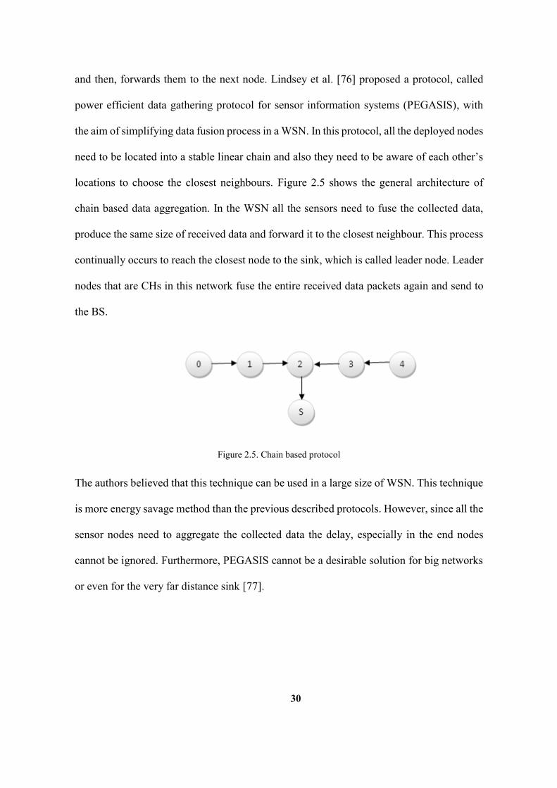
and then, forwards them to the next node. Lindsey et al. [76] proposed a protocol, called
power efficient data gathering protocol for sensor information systems (PEGASIS), with
the aim of simplifying data fusion process in a WSN. In this protocol, all the deployed nodes
need to be located into a stable linear chain and also they need to be aware of each other’s
locations to choose the closest neighbours. Figure 2.5 shows the general architecture of
chain based data aggregation. In the WSN all the sensors need to fuse the collected data,
produce the same size of received data and forward it to the closest neighbour. This process
continually occurs to reach the closest node to the sink, which is called leader node. Leader
nodes that are CHs in this network fuse the entire received data packets again and send to
the BS.
Figure 2.5. Chain based protocol
The authors believed that this technique can be used in a large size of WSN. This technique
is more energy savage method than the previous described protocols. However, since all the
sensor nodes need to aggregate the collected data the delay, especially in the end nodes
cannot be ignored. Furthermore, PEGASIS cannot be a desirable solution for big networks
or even for the very far distance sink [77].

31
2.3.2.1.2 Tree Based Data Fusion Method
Tree based methods arrange the entire sensor nodes into a tree and organize them to
be able to aggregate the data by immediate nodes in the network [74]. Then, a brief version
of data is transferred to the root node along the tree. Figure 2.6 shows the tree based
protocol. To analyse that, there is a query routing based data aggregation algorithms that is
designed based on direct diffusion. The main thought behind this method is naming the data
using information of the entire network.
Figure 2.6. Tree-based data fusion protocol
To analyse the method, there are three general phases. Firstly, the BS broadcasts
periodically messages to each neighbour and provide them with specific information such
as task type and expire time for data. Then, the sink produces control messages with the
required gradient to guide the data packet to the destination. Finally, a path reinforcement

32
method in the network selects the specific neighbours as the next hops to be able to send the
packets with a higher rate to the identified nodes.
Although there are some advantages in applying the algorithm such as reducing
communication between adjacent nodes and also cutting the additional addressing
mechanism, there are some shortages. Firstly, the energy consumption is quite high and also
the existed delay of the protocol are not avoidable especially in a large size of network.
Suboptimal aggregation tree [78] is another protocol that is more focusing on constructing
a possible minimum tree to the BS. To analyse that, there are three main sub-algorithms.
Firstly, greedy internal tree (GIT) that is to create the tree in the network gradually and
cover the entire network. In this protocol, the closest node to the sink determines a route to
the main destination. Then, all other the nodes connect themselves to the created route.
Secondly, shortest past tree (SPT) [79] algorithm that is applied in the network to identify
the shortest data route to the sink. Overlapping route is a common shortage of SPT. Shinji
MIKAMI et al. [79] suggested that aggregation tree could be an acceptable solution in the
case of overlapping routes. Finally, the last suboptimal algorithm is CNS (Centre at Nearest
Source) [78]. This algorithm gives the aggregating responsibility to the very closest node to
the BS. Then, all the other nodes forward their sensed data to the end node to be aggregated.
Since the conditions of different networks are changing, the performance of the mentioned
sub optimal algorithms are changing. For instance, any changes in the distance of the closest
node to the BS influences performance of the network.
2.3.2.1.3 Grid-Based Data fusion Method
Vaidhyanathan et al. [80] proposed two data aggregation schemes, which are grid
based data aggregation and in-network data aggregation protocols. In grid-based data

33
aggregation, the deployed sensors are not allowed to communicate with each other. The
sensor nodes that are part of virtual particular grid, transmit data packets directly to the pre-
determined data aggregator. In-network aggregating method is similar to grid based data
aggregation with two major differences. First, any sensor can be an active aggregator and
also each sensor within a grid can communicate with its neighbouring sensors [77]. Figure
2.7 shows the general structure of grid based data aggregation.
(a) In-network aggregator (b) Grid aggregator
Figure 2.7. Data aggregation methods
Figure 2.7 (a) presents the sensor nodes that are selecting the best node to be the aggregator
of the network. Then, the selected node fuses the received packets from the other nodes and
forwards them to the sink. On the other hand, figure 2.7 (b), shows that in grid based data
aggregation all sensors directly transmit data to a pre-determined grid aggregator.
To enhance the performance of the data aggregation it was suggested to make a hybrid
scheme and apply a combination of the in-network and grid-based aggregation schemes
[80]. When an event occurs, an aggregator node will be selected while they still maintain

34
the past events in their table. When a sensor detects an event, it checks its table for the
previous event and identifies the nature of it. The in-network scheme will be followed if the
sensor identifies the event as a localized event. Therefore, the best aggregator can be chosen
depend on current situations. Apart from the authors’ claim that increased energy efficiency,
complexity of the protocol in a large size of a network is a disadvantage of the scheme. In
addition, since all the data from each node is needed to be processed and transferred, the
energy cannot be efficiently consumed. Moreover, preventing data redundancy were not
taken into account in this approach.
2.3.2.2. Structure Free Based Fusion Method
Structure free based mechanisms in WSN are the attractive techniques that can be
used in environments with frequency changes [74]. The technique is more applicable for
monitoring systems that are not required any structure. There are two main challenges in
accomplishing the techniques. Firstly, as there is no pre-constructed structure, routing
decisions for the efficient aggregation of packets need to be made on-the-fly. Secondly, the
sensor nodes are not able to wait on data from any particular node before forward their own
data. That is because the sensor nodes do not explicitly know their upstream neighbours.
Many researchers, as it is surveyed in [81], have been investigated in this area for
aggregating data. The most common techniques that is going to be explored in this section
are using neural-network and fuzzy logic systems. In [82], Chen et al. proposed a data fusion
method. The algorithm uses both neural networks and fuzzy inference. The approach, based
on some information such as temperature and smoke density determines whether a fire has
been occurred. This technique enhanced the accuracy of detection however, energy
consumption and data reduction were not taken into consideration. Doolin and Sitar [83]

35
proposed a system to monitor forest fires, based on the use of WSNs. The nodes of the
system were able to sense temperature, humidity and barometric pressure. In this approach,
the energy consumption of the network was not taken into account. Yu et al. [84] proposed
a paradigm for forest fires detection. In this approach, they considered temperature, relative
humidity, smoke density and wind speed sensors in the environment to detect fire
accurately. They reduced the amount of data traffic in the network to prolong the network
lifetime. In fact, the used cluster base deployment technique to develop a WSN and lead the
CHs to aggregate the data using a neural network. Then, the CHs send the result to a node
called manager node. Thus, the node analysis the received results to be able to detect fire in
the area of interest. This approach prolonged the network lifetime but still cannot be
considered as a comprehensive solution as they used all the received data from the sensor
nodes. Thus, they did not consider duplication in the network. As a result, QoS in the
network was not fully taken into account. In [85], a variable weight based fuzzy data fusion
algorithm for WSN is proposed. The main purpose is to enhance the accuracy and reliability
of data fusion in WSN. In this approach, each CH are assigned a different and unfixed fusion
weight. The weights are changed using fuzzy logic system, based on some factors such as
delay, data amount and trustworthiness of the CHs. The lower fusion weighted CH the lower
influence the CH can make. As a result the collected fused data packets are more reliable
and accurate. The approach to some extend enhanced the QoS of the network. However, the
authors did not take the message overhead and energy consumption into accounts.
2.3.3. Routing Protocols in WSN
A routing protocol in WSN is the process of discovering, selecting and maintaining
paths from one node to another and using these paths to deliver flow packets to their

36
destinations. In the process, determining the next node to which a packet should be
forwarded toward its destination is based on given criteria. It is an important aspect of
network communication as it affects many other characteristics of network performance.
An efficient routing mechanism can become significantly complex due to the fact that it
may consider all the current conditions of the nodes in the network [86]. In this section, the
routing protocols in WSNs with fixed and mobile BS (MBS) are going to be analysed into
different sections.
2.3.3.1. Routing Protocols with Stationary BS
During the past decade, considerable research efforts have been investigated in
developing routing techniques for delivering data in WSNs. Majority of the approaches
considered QoS constrains such as energy efficiency, delay and reliability as the main
objectives. In this section, we present an overview of the most well-known protocols in
WSNs.
R. C Shah and J. M Rabaey [87] presented an energy aware routing protocol that maintains
a set of paths. The paths will be chosen randomly once the data needs to be transferred from
source to the final destination. This approach on the one hand, decreases the risk of losing
data and increases energy consumption due to maintain the paths. N Jain et al. [88] proposed
an energy-aware multi-path routing approach to spread data traffic over the nodes lying on
different possible paths connecting the source nodes to the sink. Sequential Assignment
Routing (SAR) [89] for WSNs produces multiple paths from a source node to the BS. The
path selection considers both delay and energy resources to prolong the life time. In [90] an
energy-aware routing algorithm for cluster-based WSNs have been proposed. The cost
function is defined between two sensor nodes in terms of energy conservation, delay

37
optimization and other performance metrics. Real-time and Energy Aware Routing (REAR)
[91] uses metadata to establish multipath routing to increase the energy consumption in the
network. In order to evaluate the consumption of bandwidth on the links a cost function is
constructed. The best route is then chosen, based on the relationship between the energy and
delay. The authors proved that energy consumption is reduced followed by activating image
sensors and using metadata of real data in routing setup. However, the idea of metadata
cannot be a good option as the metadata for streaming data can itself cause a huge energy
and bandwidth consumption. Ant-based Service Aware Routing (ASAR) [92] is a
hierarchical protocol that incorporates reinforcement learning to route data. In each round
of data collection, three different paths that meet the QoS requirements are chosen. Then,
the most optimal route will be maintained in a path table at each CH. The authors enhanced
QoS in terms of delay, packet loss rate and energy consumption. However, in hierarchical
models, the bottleneck problem and new optimal path setup due to congestion issue, requires
extra calculation that might decrease network performance. the issue arises in a large size
of WSNs. Zongwu et al. [93] proposed a novel genetic algorithm to satisfy the necessary
QoS parameters such as end-to-end delay, minimum cost and maximize network lifetime.
A proposed energy efficient routing protocol [94] attempt to manage both energy
consumption and delay based on AntNet protocol. This approach uses the concept of ant
pheromone to produce two prioritized queues with the purpose of sending differentiated
traffic. However, the approach cannot be a comprehensive solution due to the required
memory to save both queues. Peng et al. [95] proposed an adaptive QoS and energy-aware
routing approach. They developed a biological ant colony algorithm for WSNs with the aim
of meeting QoS requirements in an energy-aware fashion to maximize the network lifetime.
Their simulation results proved that the proposed algorithm improved the performance of

38
WSN in different scenarios. M Chen et al. [96] presented a multiple-priorities-based path-
scheduling algorithm to guarantee the end-to-end transmission delay while balancing
energy and bandwidth usage among all the node-disjoint paths in WSNs. Shu et al. proposed
two-phase geographic greedy forwarding (TPGF) [21] with the aim of minimizing the path
lengths and end-to-end transmission delay. TPGF firstly explores all the possible paths and
then find the shorten distance to forward the data packets. However, the scheme has
limitations in adaptability in large-scale, high density and frequent mobility situations.
Reference [97] proposed a routing protocol that finds the least-cost and delay-constrained
path for real-time packets. They assumed that every node knows the position of all the
sensor nodes as well as the cost of links among them in the WSN. The protocol works on
finding the path by executing Dijkstra’s shortest path algorithm. Mahapatra et al. [98]
utilized the geographic location of the sensor nodes as well. They proposed an energy aware
dual path routing scheme and aims to balance the consumption of energy in each node in
the network. E Felemban et al. [99] proposed multipath multispeed protocol (MMSPEED)
to guarantee reliability and timeliness in the WSN. The protocol uses a distributed localized
geographic packet forwarding mechanism. It requires the support of IEEE 802.11e at MAC
layer with its inherent prioritization mechanism. In this protocol, each node that uses packet
loss rate at MAC layer is responsible to calculate the possibility of each neighbour to a
destination. According to the gained probability value, each node sends a copy of data
packets to a number of neighbours to achieve a desired level of reliability. So, the
probability of retransmissions is decreased. MMSPEED improves the network life time
however, number of the hops and their available energy are not considered for establishing
routes. In Table 2.2, we compare and summarize the above-explained routing protocols for

39
WSNs based on QoS constrains. The table clearly shows that the existing developed
protocols have not sufficiently improved the performance of the WSN.
Table 2.2. Comparison of routing protocols for WSN
Routing Protocol Architecture Energy efficiency
Delay Data Packet loss rate
Inherent uncertainty Flat Hierarchical
Shah and Rabaey [87] N Jain et al. [88] SAR [89] Younis et al. [90] REAR [91] ASAR [92] Peng et al. [95] Zongwu et al. [93] Caro and M. Dorigo [13] M Chen et al [96] TPGF [21] Akkaya and Younis [97] Mahapatra et al. [98] MMSPEED [99]
2.3.3.2. Routing Protocols Using MBS
In WSN with stationary sensor nodes and sinks, the probability of significant
congestion is highly noticeable. Thereby, an excessive delays and inefficient use of
underlying resources can occur. Moreover, due to the excessive use of the sensor nodes
close to the BS, the network lifetime is reduced significantly as the nodes become frustrated
quickly. In order to provide a longer lifetime in WSNs, many new categories include motion
characteristic of WSN has been developed. In the networks, the data collector can be moving
in different directions to collect the sensed data from immobile deployed sensor nodes.
Then, the source node will communicate with the sink directly or by using fewer hops.
Clearly, in this context, there are several advantages and challenging issues that are required

40
to be addressed. The major advantage of having a data collector or a MBS is to increase the
system lifetime. Indeed, the MBS leads the network to use fewer hops to create forwarding
routes. Thus, the number of transmitted packets will be reduced and accordingly, the energy
consumption will be decreased. In the mechanism, the extra energy spent for the operation
and movement of the sink does not influence the overall network lifetime. That is because
the MBS is considered as an external to the network. For example, the MBS could be a man,
navigated vehicle or an unmanned robot that periodically returns to a fixed point to recharge
itself. Another important advantage is the reduction of the probability of transmission errors
and collisions in the network. Hence, the throughput and data reliability can be increased.
This also further decreases the energy spent at the resource constrained static nodes by
cutting the required retransmissions. In spite of the advantages, there are many challenges
and issues that need to be discussed. For example, length of physical routes for the MBS.
Since the MBS has to pass through the transmission range of the deployed sensor nodes, the
following issues can occur. Firstly, long visit latency that is due to the waiting time for each
node to be visited by the MBS. The latency also becomes worse if retransmissions will be
needed. Besides, the sensor nodes may experience significant buffer overflows until the next
contact time.
In order to analyse and improve the performance of WSNs with MBS, there is a huge range
of approaches have been developed. For example, Vlajic et al. [100] proposed a routing
protocol with a MBS and reduced propagation delay and energy consumption in the
network. The deployment strategies of WSN can be generally classified into two main
categories which are backbone based and tree based structures.

41
2.3.3.2.1. Backbone Based Structure with Mobile BS
In backbone or virtual grid structured networks, sensor nodes organize themselves
into clusters on the basis of their geographic locations. Therefore, one node per each group
may perform data aggregation and communicate with the MBS. Hence, the MBS is not
required to visit the entire deployed sensor nodes.
Under the consideration of the explained deployment methods, there are many mobile sink
based protocols that have been developed. The protocols are either random or controlled
mobility based with their considerable advantages and disadvantages. Ioannis et al. [101]
proposed purely random walk as well as a combination of random walk and deterministic
walking models. Under the purely random walk model, the following three models have
been proposed. Firstly, the MBS moves toward predefined areas with random transitions.
Secondly, the sink gives more priority in visiting less frequently visited areas and finally,
the MBS gives priority in visiting areas populated with more sensor nodes. In the
deterministic walk model, the MBS moves along a predefined trajectory within small areas.
The proposed model suffers execute complex movements with a considerable overhead as
the sensors are required to constantly update the multicast trees involving the sink. Gandham
et al. [102] proposed to dynamically relocate multiple sinks into different time rounds. The
authors used an integer linear program to determine the new locations. Results showed that
the energy consumption of individual sensors is better balanced and the overall energy
consumption of all sensors is minimized. However, this centralized method suffer a high
computational complexity of linear programming. Babar Nazir et al. [103] addressed
hotspot problem and mobile sink based routing protocol (MSRP) to prolong network
lifetime in clustered sensor nodes. The CHs within the vicinity of the sink send the collected

42
data to the MBS after CH registration processed by the sink. MBS also maintains a CH
residual energy table for predicting the next position. Sink looks into this table and moves
to the CH with higher residual energy. This ensures that the nodes near the sink have higher
energy and thus avoids hotspot problem. However, this approach is not suitable for
continuous monitoring application as CHs need to wait for the arrival of mobile sink to
deliver data packets. Xu Jianbo et al. [104] studied mobile sink based data gathering
protocol (MSDG) for clustered WSN. They adopted a joint strategy of sink mobility and
routing to realize high efficient data gathering. In this approach, sensor nodes in WSN are
divided into certain number of clusters in the monitoring area with any side length. Then,
sink by choosing the closest nodes along the path build a routing tree dynamically. After
that, CHs gather the data from the CMs, aggregate and send the aggregated data to the sink
reversely using a tree based method. In this method, although the energy consumption has
been reduced due to aggregating data, the sensors still need to consume much energy to
send data packets by using number of hops to the mobile sink. Jin Wang [105] developed
distance-based energy aware routing (DEAR) algorithm for WSNs. DEAR is a routing
algorithm that setup and maintain routes in WSNs. In setup phase, the algorithm first
calculates the distance among sources and sink nodes. If the distance is less than a
predefined threshold, the data will be directly transmitted to the BS. Otherwise a multi-hop
routing method will be considered. This algorithm also determines the number relay hops
as well as finding the closest relay node to the sink. The author believed that high
transmission power will drain a significant amount of energy from the nodes. That is
attempting to transmit over long distance, consumes more energy compared to low power
multi hop transmission covering the same distance. Apart from the advantages of this
algorithm, it increases the traffic at intermediate nodes unnecessarily. Moreover, the closest

43
node to the sink is in the high risk of losing energy. DEAR does not also measure the
available residual energy of selected nodes. This may cause the intermediate node becoming
totally drained of their energy during data transmission process.
2.3.3.2.2. Tree Based Structure with Mobile BS
This structure can be classified into source-based and sink-based structures. In
source-based structures, source nodes broadcast their information to the entire network and
create a tree-rooted for delivering data packets. Then, the MBS uses this tree to retrieve data
from the source. On the other hand, in sink-based structures the MBS broadcasts its location
to the network and assigns a tree-rooted. Nodes then, use the reverse tree path to deliver
data to the sink. Both, source-based and sink-based mechanisms have their benefits and
issues. For example, in source-based mechanism, roots creation is usually independent of
sink mobility. However, energy consumption as well as congestion are considerably high.
That is because each source node is required to be updated about the previous routes
priodically to deliver data packets. In contrast, sink-based mechanisms require only one tree
for the MBS, irrespective to the number of sources. The MBS is required to periodically
update their location for the network. These periodic location updates increase the control
traffic overhead and network’s energy consumption. To reduce these periodic sink location
updates, several solutions have been proposed [106]. Marta et al. [107] developed a method
to lead mobile sinks to be relocated once the sink noticed that energy of sensors nearby them
is depleted. The mobile sink follows paths that direct it to the node with highest available
energy. The authors claimed that an improvement by 4.86 times in network lifetime was
achieved compared with static sink case. Their proposed strategy requires that the sensors
send additional information to the sink periodically. Hence, the energy consumption as well

44
as message over head is considerably high. Yun et al. [108] developed an approach with the
purpose of maximizing the lifetime of WSNs by using a MBS. They formulated
optimization problems that maximize the network lifetime subject to delay, node energy
constraints and flow conservation constraints. In this method, each source node is not
needed to send the data immediately once it becomes available. Instead, the node can save
the data temporarily and transmit it when the mobile sink is at the most favourable location.
However, it assumes that the mobile sink needs to visit all the predefined locations in sensor
fields even if do not need to be visited. They also did not consider the emergency situations
with critical data packets.
Table 2.3 shows a comparison of different routing protocols in WSNs with MBS. The table
illustrates that all the approaches that have been explored in this section improved the
performance of WSN, but the problem has yet solved properly. That is because of the lack
of fully consideration about the local information in WSNs. Moreover, the existed
approaches did not take emergency situations with urgent data into account. Additionally,
the designed systems have limitations in dynamic environments which contain a variant
amount of noise created by some interferences.
Table 2.3. The comparison of different routing protocols using MBS with respect of QoS
Protocols Methodology Sink movement
Energy Traffic overhead
Priority visiting
Urgent of data
Inherent uncertainty
Ioannis et al. [101]
Distributed Random
Gandham et al. [102]
Centralized Controlled
MSRP [103]
Centralized Controlled
MSDG [104]
Distributed Controlled
DEAR [105]
Distributed Controlled

45
Marta et al. [107]
Distributed Controlled
Yun et al. [108]
Distributed Controlled
2.3.4. WSN Coverage Method
Solutions to coverage and deployment problems in a mobile WSN investigate how
to locate sensor nodes to meet the existing constraints and examine how well a sensing field
is monitored. In this regard, recently, there is a considerable number of protocols and
algorithms that have been developed to solve the problem. The protocols, in terms of
computational organization, can be categorized as centralized and distributed algorithms. In
centralized organizations, to process data and also local information on the deployed nodes,
a central location is required. The drawback of this method is the very high communication
costs and intrinsic delay. This becomes worse when the number of nodes in the network
increases. Consequently, the centralized algorithm is not reliable in large networks. On the
other hand, in distributed algorithms that distribute the load of computational effort across
the network, delay and inter-sensor communications are reduced. In such methods, each
sensor determines its location locally by communicating with its neighbours without the
requirement of sending and receiving location information to and from the central server.
Generally, compared to centralized algorithms, distributed algorithms are more robust and
energy efficient [109]. Apart from the computational organization, to address the research
problem and make it more understandable, in this section some of the recent developed
approaches are analysed.
46
In WSN, maintaining both coverage and uniformity is vital and there have been many
investigations with the aim of improving it. In the networks examined, it has been assumed
that deployed sensors have fixed sensing and communication ranges. Huang and Tseng
[110] proposed an efficient polynomial time solution by considering the coverage of each
sensors’ sensing range. In the literature, the coverage problem is formulated as a decision
problem with the aim of determining whether the area is sufficiently K-covered. Indeed,
every point in the areas of interest needs to be covered by at least K sensors, where k is an
integer. However, this approach does not efficiently address the problem as the uniformity
and also the number of sensor nodes were not considered. Moreover, this approach is
designed for a static environment as it is a deterministic deployment based protocol. PFRL
[111] is a probabilistic fuzzy logic based localization algorithm. This algorithm, to some
extent, by managing uncertainty associated only with received signal strength (RSS)
reduced the localization errors in WSN. In fact, PFRL improved localization accuracy in
separating mobile sensor nodes. However, the authors only managed to enhance the node
deployment process in a sensor field. They did not consider self-healing, energy
consumption and also the uniformity of the WSN deployment. Misra et al. [112] addressed
the problem of network coverage and connectivity. They proposed an efficient solution to
maintain coverage so as to preserve the connectivity of the network. The main contribution
of their research work is to cover the monitoring area by considering the overlap region and
connectivity of the deployed sensor nodes. In this process, the authors started with the two
nearest nodes in the network which guarantees the connectivity backbone formation and
then extended the backbone by activating new nodes in the communication range of those
active nodes. That would proceed until the entire area is covered. The main disadvantage of
the proposed approach is the lack of consideration of mobile sensor nodes as the approach

47
is designed for only static networks. In [113] the relationship between deploying density,
coverage and connectivity was analysed. The authors raised the sensing-coverage phase
transition (SCPT) and the network-connectivity phase transition (NCPT) problems. They
proposed a new model of combination for both coverage and connectivity. The connected-
coverage problem is approached using the theory of percolation [114], where the goal was
to probabilistically calculate the fraction of area covered at the critical density when phase
transition occurs. However, the paper does not address how to recover the coverage holes.
The main disadvantage of the research work is high energy consumption as it is a
probabilistic approach. P. M. Pradhan and G. Panda [115] presented an energy efficient
sensor deployment based on a multi objective particle swarm optimization algorithm. In this
research work, the main objectives are coverage and network lifetime within the constraint
of network connectivity. The disadvantage of the approach is a lack of consideration of
uniformity and the distances among deployed nodes. Jiang et al. [116] proposed a cascaded
movement solution for the coverage problem. They initially partitioned the area into a
number of grids. In each grid, a grid head is selected to execute the intra grid management
and inter-grid communication tasks. The grid head that detects a vacant grid will find
specific sensors in its grid and then force them to move to the vacant grid. If the coverage-
hole healing procedure fails, the grid head will further notify the grid head in its
neighbouring grid and then initiate a cascaded movement. In the literature, they enhanced
the coverage, however, the energy-balanced degree of mobile sensors and uniformity were
not taken into account as they randomly select sensors to heal the vacant grid. Qu et al. [117]
developed an efficient method for relocating mobile sensors to achieve optimum sensing
coverage. The study introduced an average distance based self-relocation and self-healing
algorithm for randomly deployed mobile sensor networks. In this approach, each sensor, by

48
sending and receiving a message, calculated the distance between each other and made
moving decisions. The proposed approach is a random based direction movement that
clearly reduces the energy efficiency in the WSN.
Table 2.4. The comparison of different coverage protocols with respect of QoS
Protocols Node Deployment
Coverage Healing
Methodology Energy Efficiency
Uniformity Inherent Uncertainties
K-Coverage [118]
Distributed
PFRL [111]
Centralized
S. Misra et al. [112]
Distributed
M. Amery et al. [113]
Distributed
M.Pradhan [115]
Distributed
Jiang et al. [116]
Centralized
Qu et al. [117]
Distributed
Table 2.4 present a comparison of different developed coverage protocols with respect to
QoS in WSN. The table shows that although they enhanced QoS in WSN, they cannot be
considered a comprehensive solution. Therefore, in this paper a distributed node
deployment and coverage-healing protocol with consideration of energy efficiency,
deployment uniformity and inherent uncertainties in WSN is proposed.
2.4. Chapter Summary
In this chapter we deeply analysed number of approaches in WSN respect to QoS
requirements. We firstly introduced WSN technologies, sensors and applications in details.
After that, the most considerable challenges in WSN were explained and analysed. Then,

49
we focused more on the existing approaches that have been developed with the purpose of
enhancing QoS in the networks. We divided the approaches into four main sections. First,
we analysed clustering approaches in the networks with explanation of their advantages and
disadvantages. Next, different data fusion methods were analysed and tried to show the
existing research gap in the existing approaches. Third, data routing protocols with
stationary and mobile sink were addressed. Finally, WSNs coverage were taken into
consideration. The approaches showed that they emphasized on enhancing QoS and
efficiency of energy consumption.

50
Chapter 3
A SELF-CONFIGURABLE CLUSTERING SCHEME IN WSN Despite significant advancements in wireless sensor networks (WSNs), energy conservation
in WSN remains one of the most important research challenges. One approach commonly
used to prolong network lifetime is through aggregating data at the cluster heads (CHs).
However, there is possibility that the CHs are failed in functioning correctly due to number
of reasons such power instability. During the failure, the CHs are unable to collect and
transfer data correctly that leads to fail the performance of the WSN. Early detection will
reduce the data loss and provide possible minimal recovery efforts. Therefore a self-
configurable clustering (SCCH) mechanism to detect the disordered CHs and replace them
with other nodes is paramount to the WSN.
3.1. Introduction
The most challenging aspect of WSN is they are energy resource-constrained and that
energy cannot be replenished. The problem arises when all the sensor nodes are required to

51
forward the data packets to the sink node. In this process, the available energy in each node
can be wasted through idle listening and retransmitting due to collisions as well as
overhearing. Cluster-based WSN routing protocols excel network topology management
and energy minimization [119]. Clustering methods in WSN lead the sensor nodes to be
organized into small disjoint groups, where each cluster has a coordinator referred as CH.
In cluster based approaches the sensors do not need to communicate directly with BS.
Instead, the CHs are responsible to organize cluster members (CMs) and send the data
collected within the cluster to the BS. This process lead to a significant reduction in the
amount of transferred data in the network. Consequently, overheads in communication as
well as bandwidth in clustering will be reduced significantly [119-122]. Figure 3.1 shows a
general view of a clustered WSN. Maintaining the created clusters is the main challenging
task in the methods. To choose a node as a CH, it is necessary to define its eligibility. That
is calculated based on local information of the nodes’ current situations such as its residual
energy. The eligibility of the selected CHs however, reduces as they sensor nodes are
consuming energy for transferring data. If the eligibility of the CHs reduce to a certain level,
they may introduced as failed CHs. In the case, the deployed sensor nodes are required to
be re-clustered. As a result, in a period of time the sensor nodes cannot collect data. The
problem arises if the failure of the CH is not predicted, which could be a sudden physical
damage. Respectively, the CMs keep sending their data to the failed CH and consequently
the data will be lost.

52
Figure 3.1. A clustered WSN
Many developed approaches investigate the problem and suggested to use backup CHs
(BCHs) [123-125]. Figure 3.2 shows a general view of a clustered sensor nodes with BCHs.
In those approaches, BCHs take over the responsibility once the defined CHs noticed their
eligibilities of being CHs are on a certain level. They proved that BCHs secure more the
created clustering formation in the WSN. These approaches however, did not address the
problem sufficiently. That is because, they mostly focused on only predicted CH failure.
The CMs in the existing approaches cannot define whether their CHs are operating or
already failed unless they received an alerting message. Those approaches did not also
consider the temporary CH failure. Moreover, they assumed that the determined BCH is
always fully functional and always is the most appropriate node to be replaced with the
defined CH. Finally, they only considered maximum of two BCH in their protocols.
However, their assumptions are not realistic. That is because, in WSN there is no guarantee
that the determined BCHs are always fully functional as the sensor nodes do not consume
energy equally. In some situations, the BCHs might be used more than the other nodes.
Also, considering maximum two BCHs is not ensuring the created cluster formation.
Specialized Sensors
Source Node
Sensor Node
Cluster Head
Base Station

53
ComputerCo
Computer
Determined CH
Backup CH
Cluster Member
Base Station
Figure 3.2. Clustering formation of sensor nodes
To overcome the issue, we propose a clustering mechanism for WSNs. In which we use
type-2 fuzzy logic system (FLS) [126] and local information of the nodes to calculate the
eligibility of the nodes. The node with maximum eligibility is selected as a CH. The other
nodes are saved on a list based on their calculated eligibilities as BCHs. Therefore there is
always a BCH for a failed CH in each cluster. To replace the BCHs with failed CHs we
consider both temporary and permanently failure in the CHs. Moreover, we take
unpredictable as well as predictable CH failure into account.
3.2. Problem Overview
Given wireless sensor nodes deployed randomly over a surface area.
The sensor nodes and BS are stationary. The clustering problem is to identify and make a
collection of CHs and CMs, while they cover the entire deployment area. Generally,
clustering protocols in WSN are divided into two main sections. In the first section clusters
are organized followed by CHs selection process. In this phase, the sensor nodes cannot
collect and transfer data packets among each other. After the clusters were created, the
sensor nodes are able to collect and transfer data to each other. They consume energy as

54
they receive and send the data packets. So, each sensor node is in the risk of being disordered
due to its energy depletion. The amount of energy lost in CHs is usually more than CMs as
they are responsible to collect data packets from other nodes and transfer them to the BS.
Therefore, they are more in the risk of energy depletion. As a result, they cannot monitor
their areas of interest. The problem becomes more challenging if the failed CH was not
detected. In the case, CMs keep sending their collected data to the CHs without noticing
that they cannot be received.
CH failure could be predicted and so, the CMs can be noticed by a message. Then, the CMs
are required to replace their defined CHs with the most optimum BCHs. However, finding
and replacing BCHs is needed to be considered carefully. In the real world, the deployed
sensor nodes are not consuming their energy equally. That means current situations of the
nodes are not changing similarly. As a result, the already determined BCHs are not always
the most appropriate node to be replaced with failure CHs. In the case, it is a considerable
challenge for the CHs to find and introduce the best current BCH to the CMs.
The problem is more challenging if the CHs are failed unpredictably. The CMs then, keep
sending their data to the failed CHs without noticing they are not received. Thus, it could
make the WSN to lose number of data packets. To prevent of the data lost in the network,
it is significantly important to determine the failure CH by the CMs at the earliest moment.
The CMs also are required to find and replace a BCH with the CH.
CH failure in WSNs could be permanently or temporarily. Permanent fault means the node
is beyond repairs and needed to be replaced to ensure the QoS in the WSN. It can be
happened due to reasons such as damaged components. Temporary fault on the other hand,
is the one that results from temporary environmental impact or incorrect state of

55
components. To replace BCHs with the failed CHs it is also necessary to realise that it is
not a temporary failure. That is because short-term lower density may not be an issue as
long as the network remains connected.
3.3. Self-Configurable Clustering
To develop SCCH, we first need to select an appropriate CH for each cluster. For
that purpose, we develop a type-2 fuzzy logic system (FLS) to find the most appropriate
CHs for the clusters. FLS is used by the sensor nodes to calculate their eligibilities of being
a CH. The input of the system are as followed;
1. Energy (E): residual energy in CHs candidates is used in electing CHs with an
acceptable energy level. All nodes are aware of their remaining energy.
2. Node Centrality (NC): is a value that shows how central the node is among its
mobile neighbours within the entire network. The lower value of the centrality,
the lower amount of energy required by the other nodes to transmit the data
through that node as CHs. NC is defined by Eq. (3.1):
NC =
where , is the distance between the CH candidate i and its
member nodes, in the number of neighbors of node i and is the size of
the sensing field area.
3. Local distance (LD): This is sum of the distances from a deployed node to its
neighbours. Figure 3.3 shows the deployed sensor node and its neighbours
within r radius.

56
Figure 3.3. A deployed node with neighbours
In order to calculate LD, we first determine the radius ( ) value as follows[4]:
(3.2)
Next, we consider only the neighbours within the confine of radius for each
node and then, sum up the distance of the node to them, as shown in the
Eq. (3.3) [127].
(3.3)
Next, the output of the FLS for each sensor node will be sent by a beacon message to
neighbours to be informed. Figure 3.4 shows the structure of the beacon message for sending
the output of FLS.
Packet Type Node-ID FLS-OUT
Figure 3.4. Eligibility of each node
Where Packet Type presents the purpose of the message, Node-ID is the ID of the node that
creates the message and FLS-OUT is the output of the fuzzy system. The nodes that have
received the message from the other nodes need to check FLS-OUT. They compare the
received FLS-OUTs against its calculated fuzzy output as well as the received other nodes’.
A Sensor node with the highest FLS-OUT introduces itself as a CH. It also lists the other

57
sensor nodes, based on their FLS-OUT. In the list, they are ordered from the highest to the
lowest FLS-OUT of the nodes. In fact, the list prioritises the sensor nodes to be BCHs.
Therefore, sensor node with lower FLS-OUT knows that it is a BCH of the node with higher
FLS-OUT. That is to ensure there is always a BCH for defined CHs. Figure 3.5 presents
structure of the CH joining message.
Packet Type CH-ID BCH-IDs
Figure 3.5. CH joining message
Where Packet Type presents the purpose of the message, CH-ID shows the ID of the elected
CH and BCH-IDs is the list of sensors’ IDs from highest to the lowest FLS-OUT. Next,
each sensor node that received the CH joining message sends an acknowledgement message
to join to the CH. Once the clusters are created, the CHs allocate a TDMA (Time Division
Multiple Access) for the CMs. Then, the sensor nodes can start transferring data packets in
the WSN based on the allocated TDMA schedule. At this stage, the sensor nodes include
CHs consume energy. As a result, either CHs or CMs might face to energy depletion. If
CHs die, the entire area of their interest will be unmonitored. Thus, replacing the failure CH
is necessary. Disordered CMs also influence the eligibility of the elected CHs as NC and
LD are affected. Therefore, to maintain the created clusters the CMs are needed to send their
residual energy with their sensory data in a single message to their CHs. The CHs also are
required to check their own FLS-OUT frequently. In each round of checking the FLS-OUT,
the CHs compare it against a determined threshold (β). If the FLS-OUT of each CH is less
than the threshold, it will be required to inform the CMs and a BCH about the switching
time. So, the sensor nodes can replace their CHs with the introduced BCH.
The available BCH cannot be fixed in the WSN. That is because the BCHs might be
physically damaged or in some situations their residual energy might be changed. Therefore,

58
CHs change the order of the BCHs in the created list based on received their residual energy.
The updated list is sent to the CMs periodically to make sure that the most suitable BCH is
available.
In the WSN the determined CHs also could be suddenly disordered due to for instance,
physical damage. If a CH dies, the CMs are required to be noticed quickly to prevent of data
losing in the network. Also if the CMs die, their CHs are required to remove them from their
list. To achieve that, we propose to monitor the CHs and CMs using TDMA. Figure 3.6
presents the allocated TDMAs for .
As it can be seen from Figure 3.6 (a), the CMs need to transfer their data packets upon
receiving a data request message (Data-Req). If the CH did not receive the requested data
at the end of the frame, it will mark an error for the CM. the error mark is to prevent of
assuming the temporary dead as a permanent failure. Then the CH sends another request. If
the CH did not receive data from the CM by the end of the frame it will check the error
mark. If the error mark is existed, the CH realises that it is a permanent failure and it needs
to be removed from its CMs’ list.

59
Slot time Si
Time
Data-Req Data-ReqIF Not Recv-dataMark Er(i)
Slot time Si
IF Not Recv-dataIF Er(i) exists
remove Si
Slot time Si
Wait for Data-ReqIF No Data-Req
wait for next Data-Req
IF No Data-Reqsend joining message to BCH
Slot time SiTime
(a)
(b)
Figure 3.6 Allocated TDMAs for (a) CH and (b) CM.
Apart from the CM, failed CHs are also needed to be detected. Figure 3.6 (b) presents the
TDMA of the CMs. The CMs in the WSN need to wait for a data request (Data-Req) from
its determined CH. if it does not receive Data-Req, it will wait for the next frame to receive
the request as it might be a temporary failure. In case of not receiving the request in the
second frame, it will be required to replace its CH. To replace the CH, the CM needs to
check the latest and updated of its BCHs’ list. Then it sends a joining message to the first
available BCH and waits for acknowledge message. However, there is a possibility that the
defined BCH might be disordered. In the case of not receiving the acknowledge message
from the BCH, the CM sends another joining message to the second available BCH until it
joins to a CH.

60
3.4. Performance Analysis
In this section we evaluate the performance of the proposed shame using simulation.
As a performance metric, we compare the efficiency of energy consumption of the
networks. The communication model for energy consumption used in this evaluation is as
explored in [66]. The transmitter dissipates energy to run the power amplifier and radio
electronics is shown in Figure 3.7.
Figure 3.7. Radio energy dissipation model
The required energy for transferring a k-bit message to d distance can be calculated by using
(3.4).
(3.4)
Energy consumed in receiving k-bit message can be computed by (3.5). Where based on the
referred algorithm = 50nJ/bit and = 100pJ/bit/m2.
(3.5)
Apart from energy consumption, we analyses data loss ratio (DLR) of our proposed
approach. DLR is a ratio of the difference of total data sent by the sensor nodes and received
by the BS to the total data sent by the sensor nodes as provided below;
61
(3.6)
Finally, we analyse the traffic overhead of our proposed protocol. To evaluate the traffic
overhead of the distributed approach in WSN, we tested the average amount of traffic
transmitted within the network
3.4.1. Experimental Setup
In this section we use MATLAB to compare our proposed approach against PDD
(Probability, Distance and the sum of Distances) [128] and Achieving Reliability over
Cluster-Based WSN using Backup Cluster Heads (DBCH-LEACH-C) [129]. The reason
behind choosing PDD is that it is a fuzzy based approach that increased the network lifetime
and DBCH-LEACH-C is also a clustering WSN that proved using BCHs enhances
performance of the WSN.
In the simulation, the network consists of a BS and 80sensor nodes, ,
wireless sensor nodes. The sensing range for each sensor is 25m and the communication
range is 50m. The sensor nodes are deployed randomly over 200 * 200 meters surface area.
The initial energy for each node is 1J equally. In terms of energy, memory and
computational power, there is no limitation for BS. BS is located in the middle of the
surface. The packet size is 100 bytes and beacon message is 10 bytes.
3.4.2. Result and Discussion
Figure 3.8 compares the rule surface of our scheme and PDD. Based on the plotted
surfaces, the chance of finding CHs in the network by our system figure 3.8 (a) is higher

62
than PDD figure 3.8 (b). Moreover, our system introduces a substantially smother surface.
This smooth response will consequently provide a better monitoring performance that can
handle the uncertainties although, the complexity of the system with respect to the size of
the fuzzy rule based is remained the same (no additional fuzzy rules or fuzzy sets were
used).
(a) Our proposed system
(b) PDD

63
Figure 3.8. Comparison of the response surface generated by the Fuzzy systems
In order to prove that the proposed approach prolongs the network’s lifetime, we calculate
the required energy for successful transmission of specific number of data packets. As can
be seen from figure 3.9, the results show that the proposed approach outperforms both PDD
and DBCH-LEACH-C by transferring the same amount of data with less energy dissipation.
PDD has the less efficiency in energy consumption. That is due to the lack of consideration
of CH and CM failure in the network. In case of CH failure, CMs transfer data packets
through the networks without noticing they cannot be received. As a result, the efficiency
of energy consumption is negatively influenced. DBCH-LEACH-C enhances PDD as it
replaces BCHs with the failed CHs.

64
Figure 3.9. Energy consumption
However, as it is a centralized protocol and did not consider the CM failure energy cannot
be consumed efficiently. That is because; the network needs to consume energy to make a
data request from a CM by a CH without noticing the CM is already disordered. SCCH on
the other hand, enhances the energy efficiency in the network. The reason behind it is
because SCCH is a distributed protocol, in which the CHs and CMs of a cluster can define
whether they are failure of not. In case of CH failure, the CMs are able to replace the most
optimum BCH with it. As a result, data request message as well as data packets are not
transferring unless the nodes are ensured that the destination node is fully functional. Apart
from energy consumption, data loss ratio (DLR) is calculated for the data sent and received
at the BS for the whole network. As illustrated in Figure 3.10, SCCH has the lowest DLR.
Figure 3.10. Data loss rate
That is due to the following reasons. First, it can determine failure of CHs and CMs. That
prevents of transferring data packets to a failure nodes. However, CMs failure is not
considered in both PDD and BCH-LEACH-C. In addition, there is always a BCH for a

65
failed CH. So the CMs do not need to worry about re-clustering process as they can simply
replace a BCH with their determined CH. BCH-LEACH-C performs better than PDD as it
considers BCH. However, its DLR is lower than SCCH that is due to considering only
maximum two BCHs.
Finally, traffic overflow is also used to prove the performance of the proposed approach. In
order to evaluate traffic overhead of SCCH, we tested the average amount of traffic
transmitted within the network. Figure 3.11 compares the average message for transferring
data with different sizes of network. It clearly shows that the traffic in our scheme is lower
than PDD and BCH-LEACH-C. The message in PDD is more than BCH-LEACH-C and
SCCH because in case of CH failure the nodes are required to be connected to the BS
directly.

66
Figure 3.11. Message Overhead in cluster
3.5. Chapter Summary
To prolong WSN lifetime as well as decreasing the created traffic in this chapter, we
proposed a new distributed type-2 fuzzy based self-configurable clustering (SCCH)
mechanism. SCCH firstly clusters the sensor nodes. That is followed by selecting CH. To
define CHs we used a fuzzy system and considered local information of each sensor node.
The output of the system is presenting the eligibility of sensor nodes to be CHs. Then, nodes
in the network compared their eligibility against others’. A node with the maximum
eligibility will introduce itself as a CH and the rest of the nodes as BCHs. As a result, the
CMs can ensure that there is always a BCH for their CHs. Therefore, in case of CH failure
the CMs can replace the BCH with the permanent CH failure. The claim was proven by
comparing the behaviour of the SCCH against a fuzzy and a well-known non-fuzzy
approach. It achieves longer lifetime with the ability of reducing overhead in WSNs,
compared to existing clustering protocols.
For the future work, we would like to extend the protocol to meet QoS requirements of
WSNs, such as coverage preservation, because complete coverage of the monitored area
over long period of time is an outstanding issue. Also, since, the amount of uncertainty in
different environment is not the same Thus; obviously, a certain fuzzy interval cannot be
used in different applications. Therefore, it is necessary to come up with a method to be able
to estimate the best fuzzy interval for the membership functions.

67
Chapter 4
A DATA FUSION METHOD IN WSN
The success of a WSN deployment strongly depends on the QoS it generates about the
events of interest. Low data quality is a prevalent problem in WSNs, which is due to a
variety of reasons such as sensor failure or data duplication. This is especially challenging
in data fusion mechanisms, where a small fraction of low quality data in the fusion input
may negatively impact the overall fusion result. To provide a higher quality of fused data a
distributed data fusion mechanism is proposed. The proposed algorithm is able to
distinguish and aggregate only true value of data instead of processing the entire data. It is
generally divided into three main phases. Firstly, to differentiate the true value of data from
other data a fuzzy logic controller (FLC) is developed for each sensor. After that, the cluster
heads (CHs) fuse the received data. They are also responsible to calculate and then, send
the probability of occurring the target events in the monitoring area to the base station (BS).
In this process redundant data is simply eliminated and consequently, energy consumption

68
is reduced. The transferred data are then stored in the BS. To detect the events the BS needs
to analyse the history of the received data. If a trend of change in the received data is noticed,
the BS can determine whether the events occurred. In such a case, BS reports the detected
event to the alerting system.
4.1. Introduction
In WSNs, sensor measurements are referred to as a sensor reading or sensor value.
The corresponding correct value of an event in the environment of the data is referred to as
the true value. If a sensor reading and the true value disagree, the sensor reading is said to
be incorrect. The error that leads to an incorrect sensor reading can occur at a sensor node
level. A sensor node itself might in some cases collect incorrect data. Moreover, duplicating
data might also decrease the QoS. In order to overcome the problem, a data fusion
mechanism is required to be developed to remove the incorrect data as well as duplicated
data in the data fusing process.
The main purpose of data fusion mechanism in WSNs is to provide a greater QoS for the
purpose of making reliable and accurate decisions about the events of interest. Data fusion
mechanisms process the data from multiple sensors and thereby create meaningful new
information that cannot be obtained from any single sensor. In fact, fusing data ensures that
not only the data quality of the WSN is enhanced but also energy consumption can be
lowered as it removes redundant information [73].
There are many data fusion mechanisms with the purpose of reducing the energy
consumption in the WSN [130-132]. These mechanisms used different techniques such as
probability theory [133], fuzzy set theory [134], possibility theory [135], rough set theory

69
[136] and Dempster-Shafer evidence theory (DSET) [137, 138]. Most of these approaches
are able to eliminate duplicated data in the fusing process. However, these approaches do
not consider specific limitations of the sensor devices. In fact, they assume that the entire
received data from sensors are the true value, which is an unrealistic assumption. Moreover,
all existing schemes transfer include both necessary and unnecessary data to the BS. As a
result, energy consumption is quite high.
The goal of the proposed sensor data fusion approach is to improve the performance of a
system with respect to the level of QoS generated about the events of interest. Moreover,
by transferring only the necessary calculated probability of the events instead of the entire
fused data to the BS energy consumption is minimized. Finally, the proposed approach is
robust in terms of sensor node failures as it combines all the received data from the sensor
nodes to measure the events of interest.
4.2. Research Problem
To avoid heavy traffic and conserve energy in a WSN caused by the transmission of
unnecessary data packets to the BS from each sensor node, a data fusion method can be used
in such networks. A data fusion method in a node is used to aggregate the received data
from the other sensors. A general block diagram of a data fusion mechanism is given in
Figure 4.1. The sensor nodes collect data from the environment.
They then send the data to a fusion node. Next, the node will create one single internal
representation of the environment from its inputs. The single representation is then
consumed by the BS. This means that the BS in general does not have access to the
individual sensor measurements.

70
Environment
s1
s2
s3
Fusin Node
BS
D1
D2
D3
U
Figure 4.1. Fusion mechanism
In many situations depend on the current conditions of the sensor nodes,
might not be exactly the true value. There are many useless data packets generated and
transferred from each sensor node in each round of data collection. In many situations, a
sensor node is not able to recognize the useless data while it generates data packets for
further process. The data are transferred to the fusion node and aggregated with the others’
true value of data. As a result, they can effect negatively in making accurate decisions as
well as efficiency of energy consumption in the WSN. To solve the problem it is necessary
to address the unnecessary data in addition to redundant data transferred from sensor nodes.
To formulate the problem, we consider a set of sensors in a cluster based WSN deployment.
These sensor nodes collect data and then send it to their CHs. CHs are responsible for fusing
and transferring the data to the BS. The problem of data fusion can be formulated as follow:
Maximise (4.1)
(4.2)

71
(4.3)
The objective (4.1) is to maximise the network life time ( ) subject to maintaining or
enhancing quality of the produced data. Constraints (4.2) and (4.3) ensure that the
percentage of collected true value of data ( ) and data redundancy ( ) are satisfied by a
user-defined threshold.
4.2.1. Data Quality
In order to enhance QoS in the WSN, it is necessary to make sure that sensor
readings and measurements are true values to be used. The main cause that makes a WSNs
produce and process incorrect data is the sensor nodes. Different environmental factors such
as a sudden change of tempest or humidity influence a sensor node behaviour. These
environmental factors decrease or increase the output signal of the sensors, which create an
ultralow-frequency noise on the transferred signals [24]. In addition, non-operating
environmental limits such as a high or low temperature of air surrounding the sensor nodes
usually influence the sensors’ performance. The operating temperature range is the length
of ambient temperatures given by their upper and lower extremes, within which the sensor
nodes maintain their expected accuracy [139].
In different WSN applications, it is impossible to confirm that the collected data are true
values of the events without taking samples or analysing data history [24]. Therefore, we
suggest to assign a weight for each collected data. The weights are determined based on
current storage conditions of the source nodes. If the sensor nodes are not in the expected
condition as revealed in their data sheets, the determined weights are changed. The better
condition a sensor node is the higher weight is assigned to its collected data. In fact, the

72
weights show the percentage of correctness of the data. Based on the calculated weights,
the correct value of data can be distinguished and separated from others. As a result, a higher
QoS can be received by the BS. Eq. (4.4) presents the percentage of the accurate received
data packets from an event by BS.
(4.4)
Where, R is the percentage of the received correct data by BS. L is the total number of
events defined by the application and is the number of messages that contain only the
received true value of data.
4.2.2. Data Redundancy
Redundancy in WSNs is defined as the use of redundant data, e.g. extra bits to report
the events of interest. Obtaining information for a specific event in a location from different
sources decreases the quality of collected data. Sensor nodes in a WSN are typically
deployed densely and thus they provide a large amount of redundant and duplicate data.
That causes serious packet collisions, bandwidth waste and energy consumption. Therefore,
removing redundant data enhances the overall quality of the collected data and minimizes
the number of transmissions from source nodes to the BS. The key idea is that instead of
expecting each sensor node to send messages for each event individually, their data can be
combined and transferred with lower traffic. Therefore, we suggest to calculate only the
probability of the events to the BS. Next, send only the necessary information out of the
entire calculated probabilities to the BS. The necessity of the obtained information is
determined based on a trend of changes. If the probability of existing events is more than a
pre-determined threshold, the system will send the information to the BS.

73
4.3. Data Fusion Algorithm
Figure 4.2 shows the proposed data fusion and transferring process. At the first step,
the sensor nodes collect data as well as calculating a confidence factor (RF) for each
collected data packet in each round. To calculate RF, a fuzzy logic controller (FLC) is
programed on each sensor node individually.
Data1 &RF1
Cluster Head
FISFIS Changes in Results?
Collection of FIS OutputsC
Yes
No
Base Station
No
Yes
Reasoning About Events
To Alerting System
Dat
a F
usio
n
Data2 &RF2
Data3 &RF3..
DaDDDD ta1 &RF1
DataD 2 &RF2
DDataD 3 &RF3..
Sensor Nodes
Figure 4.2. Proposed flow chart
FLC is developed based on Sugeno method [140]. The purpose of FLC is to find a
confidence level of the collected data considering the current condition of the sensor nodes.
Figure 4.3 shows the proposed FLC in a sensor node.
Fuzzy Inference Engine
DefuzzifierType ReductionFuzzifier
Type-2 Fuzzy Knowledge Base
Temperature
Humidity Rate
Signal to Noise
FuzzyInferenceEngine
DefuzzifierType ReductionFuzzifier
Type-2 Fuzzy Knowledge Base
aaate
ooiiise
FLC
Confidence Factor
Figure 4.3: Proposed FLC
FLC considers the non-operating temperature (T) and humidity (H) range to create the
membership functions. A random membership function is also used for noise to signal ratio

74
(N) of the sensors. FLC produces a confidence factor ( , , …, ) for each sensor
data ( , ,…, ) that is collected in a real time. The FLC in a real time, determines
whether the temperature and humidity rates of the sensor nodes and also the signal to noise
ratio are in the acceptable range. To accomplish that, FLC compares its input measurements
with the desired range for each sensor. The desired range for each sensor can be found on
its specified datasheet. The output of FLC for each sensor can be 100% only if the
environmental factors are in the desirable range.
In case of being out of the range, FLC produces a confidence factor (0% 100%) for
the collected data. Next, each node compares the calculated RFs against a predetermined
threshold. If the created factor of each data is less than the threshold value, the data will be
disregarded. Otherwise, it will be sent to CHs in a data message. This prevents the
occupation of the correct value of data by the other data that does not present the true values,
which is shown in Eq. (4.2). For fusion purpose, the message also consists of a Node-ID of
each source node.
At the second step, Eq. (4.3), CHs are responsible to aggregate the received data from the
cluster members. The data fusion process is started by CHs at the end of each round of data
collection. Eq. (4.5) is used to aggregate the entire received data from cluster members in
the same kind with different locations.
(4.5) Where is the received data from the same kind of cluster members, is the calculated
confidence factor of the collected data and FD is a combination of the data from the same
kind of sensor nodes. In fact, FD is a combination of the data with a higher certainty as it

75
combines the entire correct received data based on their confidence factors. As a result of
considering different sources of one kind of sensor nodes in different locations, FD provides
a better view of the environment. FD is also robust as data from multiple sensors with their
own confidence factors mitigate the problem of sensor failure. FD is calculated for the three
kind of deployed sensor nodes individually. Therefore, that would be a set of FDs. Next,
FDs are stored in a matrix with one row and m columns ( ). Equation (4.6) presents
matrix.
= { } (4.6)
As an example, consider three temperature, four light and three smoke density sensors. They
are deployed on a cluster-based method. Over a period of time, the temperature sensors
sense the environment by 20 ̊c, 15 ̊c and 10 ̊c with the confidence factors of 0.75, 0.65 and
0.41 respectively. As a result, the fused temperature data would be 15.93. Fused light
detector and fused smoke density data also are 49.8 and 33.2 respectively.
Based on this matrix of the monitoring system is = {15.93, 49.8, 32.2}

76
Figure 4.4. Event probability in FIS
Then, the vector will be fed and processed by a type-2 fuzzy inference system (FIS) in
CHs. The output of the system is the probability of occurring events in the monitored areas.
FIS analyses the vector based on a provided fuzzy rules after data fusion process was
accomplished. Figure 4.4 presents an example of calculating the events occurrence by FIS.
If the calculated probability in the clustered nodes was not changed, the CHs do not forward
the data packet to the BS. Otherwise, the CHs send the probability of the events in their
controlled areas. However, the change in the probability does not guarantee a correct
detection and it is only considered as a possible event in the monitored area. Therefore, to
make sure that the detection is accurate enough, the BS needs to regularly monitor and
process the received probabilities that are generated over the time. In fact, all the received
probabilities are constantly processed by the BS. If a constant change is noticed, the event
will be reported to the alerting subsystem by BS. Otherwise, the algorithm continues
collecting data. The following algorithm explains the proposed data fusion process.
1. INPUT: (T: Node temperature, H: Humidity ratio, N: Noise to signal) 2. OUTPUT: Fused Data 3. BEGIN 4. WHILE (Event NOT Detected ) 5. FOR all the cluster members in one kind 6. ← FLC (T, H, N) 7. IF 8. Data and will be sent CH 9. ELSE 10. Collected data will not be considered 11. END IF 12. END FOR 13. ← Received data by CHs from one kind of node will be fused 14. Detection Probability ← FIS ( ) 15. IF the probability was not changed 16. Disregards the received data 17. ELSE IF 18. Send the Detection Probability to BS 19. IF the event detected by BS
Algorithm: Data Fusion Algorithm

77
20. Report the event 21. END IF 22. END IF 23. END WHILE
END Algorithm
4.4. Application
The application of the network can be in a forest fire detection system that requires
measurements from in-field deployed sensors. In this application, the three different sensors
that are responsible for measuring temperature, smoke density and light are clustered in the
area. Then, each node, based on their current situation, uses FLC to assign a weight for their
data. Next, the data are sent to CHs, which is connected to MBS wirelessly. Figure 4.5
shows an example of forest fire detection.

78
Figure 4.5. Forest fire application
4.5. Performance Analysis
In the simulation, we focus on the expected amount of colleting correct data respect
to QoS in WSNs. In each round, many number of data packets are generated but it is not
necessary for the entire produced data to be sent.
To evaluate the proposed approach Eq. (4.4) is used. We also estimate the created traffic
overflow in the simulated WSN. The traffic overflow is calculated as the following:
(4.7)
Finally, we calculate the energy consumption in each round of data collection using the
method proposed in [66].
4.5.1. Experimental Setup
It is assumed to use MTS420/400 sensor board and a BS which could be IRIS with
ATmega1281 processor and a mib520 programming base. The sensor board consists of
humidity, temperature and light sensor as well as a communication component. By using
the obtained information from the device’s datasheet, MATLAB was used to implement
and analyse the performance of the network. Table 4.1 presents the obtained information of
MTS420/400. In order to simulate noise effects in real sensors, a random high-frequency
noise signal is added to the sensor signal.

79
Table 4.1. Parameters of MTS420/400
Parameters MTS420/400
Temperature Range Humidity Range Signal to Noise Ratio
−40 to +123.8°C 0 to 100% RH 0 to 1 db
The results of the experiment are compared against WSNs and fusion information methods
for forest fire detection (FIM) [141] and a variable weight based fuzzy data fusion algorithm
for WSN (VWFFA) [85]. The reason that we choose FIM is because it is a distributed
threshold based algorithm that uses MTS420/400C sensor boards as well as our proposed
algorithm. VWFFA is also chosen because it is a distributed fuzzy based data fusing
algorithm that enhances the QoS in WSNs.
4.5.2. Result and Discussion
To evaluate the proposed algorithm the percentage of correct data collected is
calculated. Figure 4.6 presents a percentage of correct collected data by BS in the proposed
approach as well as FIM and VWFFA in each collecting round of data.
As can be seen from Figure 4.6, the proposed approach provides a higher percentage of
correct data compared with the other approaches. That is due firstly, to the elimination of
the incorrect data to prevent corrupting the true value data in the fusion process. Moreover,
in the fusing process data is processed again in CHs assess whether there is any change in
the collected data.
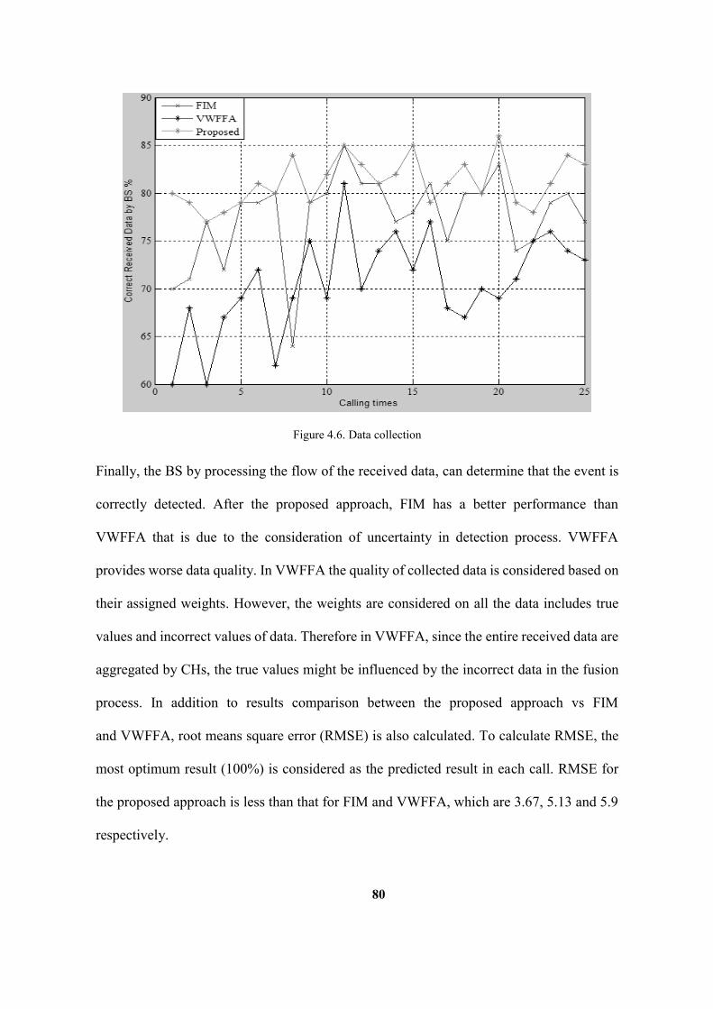
80
Figure 4.6. Data collection
Finally, the BS by processing the flow of the received data, can determine that the event is
correctly detected. After the proposed approach, FIM has a better performance than
VWFFA that is due to the consideration of uncertainty in detection process. VWFFA
provides worse data quality. In VWFFA the quality of collected data is considered based on
their assigned weights. However, the weights are considered on all the data includes true
values and incorrect values of data. Therefore in VWFFA, since the entire received data are
aggregated by CHs, the true values might be influenced by the incorrect data in the fusion
process. In addition to results comparison between the proposed approach vs FIM
and VWFFA, root means square error (RMSE) is also calculated. To calculate RMSE, the
most optimum result (100%) is considered as the predicted result in each call. RMSE for
the proposed approach is less than that for FIM and VWFFA, which are 3.67, 5.13 and 5.9
respectively.
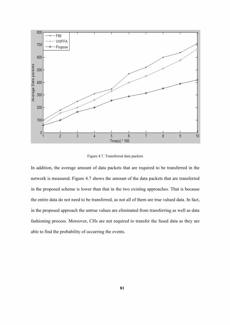
81
Figure 4.7. Transferred data packets
In addition, the average amount of data packets that are required to be transferred in the
network is measured. Figure 4.7 shows the amount of the data packets that are transferred
in the proposed scheme is lower than that in the two existing approaches. That is because
the entire data do not need to be transferred, as not all of them are true valued data. In fact,
in the proposed approach the untrue values are eliminated from transferring as well as data
fashioning process. Moreover, CHs are not required to transfer the fused data as they are
able to find the probability of occurring the events.

82
Figure 4.8. Energy consumption
The CHs send the calculated probability only if it shows an abnormality based on the history
of data. So, the data that is sent to the BS is going to be only the possibility of the detected
fire. In contrast to the proposed approach, FIM has the highest number of data packets that
need to be transferred in the network. The reason behind that is the entire incorrect and
correct collected data and also redundant data are needed to be transferred. VWFFA has a
lower transferred data number in the network than FIM. The reason behind that is the
developed network is a cluster based and the data are fused based on the assigned weights
on clusters. In VWFFA, the assigned weights reduces the influence of the incorrect data on
the true values in the fusion process.
Energy consumption is also a critical feature of a developed WSN. As explained in details,
we reduced the transferred data packets in the network. This helps significantly to reduce

83
the energy consumption. Figure 4.8 illustrates the energy consumption in the networks. As
it can be seen, the proposed scheme minimizes the energy consumption in WSN. That is
due to firstly, the lower transferred data packets in the network. Moreover, data packets
similar to VWFFA are sent to their CHs consequently, lower energy is required compared
to FIM.
4.6. Chapter Summary
The main purpose of this chapter is to come up with a quality based method for data
fusion to provide a better QoS. In the proposed approach, which was a cluster based
network, cluster members were required to collect data from the environment frequently
until a target event is detected correctly. Since they needed to make sure that their data are
true values, FLC was developed for each of them individually. FLC with the inputs of some
information of current conditions of the sensor nodes such as a temperature and humidity
ratio, determines a confidence factor for each individual collected data. Based on the factor,
each sensor could group their data into true valued and untrue valued data. Next, clearly,
the valued data was sent to CHs for further process. Then, the CHs were responsible to
aggregate the received valued data. Instead of sending the fused data to the BS, they were
required to send the calculated probability of occurring the events in their monitored areas.
To calculate the probability, each CH was equipped with a fuzzy inference system with the
inputs of the three different fused data and output of the occurrence possibilities. Next, in
case of noticing any changes in the calculated possibilities, they sent the fuzzy output to the
BS. However, the BS still was needed to process the received data with the aim of realizing
whether the detection is accurate enough. Then, the BS was required to record the detection
to the alerting subsystem.

84
Chapter 5
ROUTING WSN DATA
In this chapter, we propose two routing protocols to improve wireless sensor network
(WSN) performance and lifetime. The first approach is based on a fixed base station (BS),
in which each source node has to find a path to the BS to forward their collected data. The
second approach is based on a mobile BS (MBS) with flexible visiting routes to prevent
same nodes frequently participate in forwarding data. The direction of the MBS is controlled
and changed based on sensors’ local information.
5.1. Introduction
A routing algorithm is a process of discovering, selecting and maintaining paths
from one node to another and using these paths to deliver flow packets to their destinations.
An efficient routing mechanism can become significantly complex due to the fact that it is
necessary to consider current condition of each neighbour to be able to find the most optimal
path [119].

85
Routing protocols can be classified into three main classes: proactive, reactive and hybrid
routing protocols. Proactive-based routing protocols establish paths and keep them active
from all the sensor nodes to the sink during the networks’ life time. Then, source nodes
forward their collected data packets through the determined paths to the BS periodically. In
reactive routing protocols, source nodes need to determine a path for their collected data.
For example, Direct Diffusion routing protocol [142] calculates the best route from a source
node to the sink once a required message received from the BS. These routing protocols can
be used for query-driven applications. Finally, the hybrid routing protocol is a combination
of both proactive and reactive routing protocols.
Although there are many routing techniques for WSNs they are based on a set of
assumptions that are not realistic. For example, the effect of noise on signals cannot be
avoided in processing data by the nodes [143]. Therefore, we extend the T1 fuzzy route
management design via incorporating the Interval Type-2 (IT2) fuzzy logic [17].
We develop two routing protocols for WSNs. First, we develop a routing protocol for
stationary sensor nodes and a BS subject to enhance efficiency of energy consumption. In
this protocol delivery routes for delivering data packets from sources to the BS are
established. To define the routes residual energy, buffer capacity and congestion at each
node as well as distances among sensors and the BS are considered. Then, we extend the
routing protocol with replacing the stationary node with a MBS. We proposed a data
collection scheme (IDCS), in which MBS is responsible to visit source nodes to collect data.
Thus, the source nodes are not required to worry about establishing routes to transfer data.
Visiting time and location are controlled by a fuzzy system. The fuzzy system dynamically
prioritises the source nodes that are needed to be visited. The source nodes even have the

86
ability to call the MBS to be visited. Thus, in case of emergency situation, the source nodes
ensures that their collected data can be reached by the MBS quicker.
5.2. Problem Description
The main objective of developing a routing protocol is to enhance efficiency of
energy consumption in WSNs. Routing protocols in each data collection round are
responsible to find a relay node for transferring data packets. To find a relay node there are
many requirements that need to be taken into account. First, residual energy of the next hop.
Low residual energy of a node may cause a disconnection in the created route as it is in the
risk of failure. Next, buffer capacity is also playing an important role in choosing an
immediate node.
Table 5.1. Notations
Symbols Definitions Current residual energy of each sensor node
Network lifetime S Set of deployed sensor nodes d Distance among the sensor nodes and BS B Buffer capacity
if the location of sensor is a sojourn location of the MBS; Otherwise,
and Minimum and maximum sojourn of the sink at location Maximum tolerable end-to-end delay
If a buffer capacity of nodes is at the certain level, they might not be able to store
the received data packets. As a result, the network faces to data loss. Additionally, delay in
transferring data is another challenging point in developing routing protocols. To reduce
delay in receiving data from sources, the shortest and the most secured route needs to be

87
determined. Resubmission of data that could be due to node failure or data collisions
increases delay in data transferring. Table 5.1 presents the notations used in this chapter.
5.2.1. Problem Formulation
Distributed routing protocols in immobile WSNs lead the source nodes to find the
most suitable neighbour node as a relay node to transfer the data. To establish a route for
data, each source node needs to find a relay node subject to decrease the energy
consumption. Developing packet routes in an immobile WSN is formulated as follow:
Maximize (5.1)
(5.2)
(5.3)
The objective (5.1) is to maximize the network lifetime. To achieve that, we refer to the
residual energy of the relay nodes and their traffic rate. Constrain (5.2) stands that it is
essential to make sure that the residual energy of the elected relay nodes is more than a
certain level. Constrain (5.3) ensures that transferring rate of the selected relay node is more
than a determined threshold.
We then extend the problem by replacing a MBS with the stationary BS subject to reduce
energy consumption and transmission delay in the WSN. In this approach we use the cluster
method explained in chapter three to create disjoint groups of sensor nodes. The MBS starts
from and returns to a location to recharge petrol or electricity. The location ( may
be outside of the monitored region. During its tour, the MBS sojourns at each chosen
location for a certain duration in order to collect the sensing data from source nodes. End to
end delay time for a data packet to be delivered from a source node ( ) to the MBS, is

88
presented as . End to end delay that is calculated by (5.4) includes the delay
among cluster members (CMs) ( ) and the delay between the cluster heads (CHs) along
the path to the MBS. It is assumed that is the same for all the CMs. The delay between
CHs to reach the MBS is basically depends on the propagation delay ( ), which is the same
for all the CHs and number of data packets ( ) between the CHs and MBS.
(5.4)
We formulate the data collection scheduling (IDCS) as follows:
(5.5)
for any S (5.6)
Constrain (5.8) stands that it is essential to make sure that sojourn time for MBS is not more
than the maximum tolerable end-to-end delay otherwise, it negatively influences the rate of
packet drop. Constraint (5.6) ensures that the visiting time for MBS of CHs is limited to
ensure the entire data packets are collected, while there is always a maximum time as the
other CHs are awaiting to be visited.
5.3. Reactive Routing Algorithm
In this section we first describe the routing protocol for a WSN with stationary BS.
The algorithm starts when the BS broadcasts a data request message. All the nodes that are
idled and located in the area of interest will wake up to process the message. If the request
is not for them, they will go to sleep mode again. Otherwise, they will check their current
conditions based on their local information. To calculate that we developed a Type 2 fuzzy
logic system (FLS1). The inputs of the system are residual energy, required energy for the

89
operation and their current queue size or congestion rate. To calculate the existing
congestion, arrival and transmission rate of each sensor is calculated. Eq. (5.7) shows the
network rate of transferring in a sensor node [144].
(5.7)
Where is congestion rate of the sensor node, is the arrival data rate and is the
transmission rate of the networks. The output of the FLS1 determines one of the three next
processes. First, if the output of the FLS1 is more than , the requested data will be delivered
to the BS directly. Additionally, the energy consumption of the resource nodes and also the
neighbours for delivering data and processing the order message will be calculated. The
energy consumption is calculated based on Heinzelman's energy model [145] as it is
explained in chapter three. Secondly, if output of FLS1 is less than the collected data will
be lost as the node is not capable to deliver that. Finally, if the output of FLS1 is in between
and , the source will need to find another node to relay the data packets. To find a relay
node, there are two main steps that are updating neighbour list and finding the most eligible
neighbour for relaying data packets.
Consider a source node ( ) and its neighbours. To find a relay node, we develop another
fuzzy system (FLS2) with three inputs; residual energy, distance to neighbours and the
current congestion at the neighbour nodes. To calculate the distances among the sensor node
we used received signal strength (RSS). RSS is the measure of voltage by received signal
strength indicator (RSSI) circuit of the sensor node. Since there is no additional hardware
required to calculate the mentioned parameter, RSS measurement is not a difficult and time
consuming task for each node. After measuring the RSS, the theoretical models are usually
applied to convert the RSS into a distance estimate [146].

90
Sj
SiSs
SiiiiiiiiSSSSSSSSS
SSjjjjjjjj
ssssssssssssssss
R2
R1
Figure 5.1. T shows and compares the distance from A and B
Figure 5.1 shows how sensor node that is located in different distances from two nodes
in WSN. In the first step, RSSI value will be measured by sensor nodes to calculate the
distance can be calculated. Eqs. (5.8) and (5.9) can be applied to calculate distances based
on RSSI [147].
(5.8)
(5.9)
where RSSI is the received signal strength, d is the distance between the nodes and n is the
damping coefficient of the signal and A is the absolute value of the signal strength with 1m
distance between the transmitter and the receiver.
Then, the neighbours will send the output of the FLS2 to the node “ ” periodically. That
helps to update the forwarder table and remove the recent failure nodes from the list. Then,
the source node will select the most eligible neighbour. After the selection process, the
source node broadcasts a request message (64 bit) and wait for a reply within a certain period

91
of time. If it did not receive any ACK from the selected neighbour, the source node chooses
the second highest qualified neighbour node. When a node from the list of source node is
selected and received the data packets, the neighbour will be the new source node. The
following algorithm is the presented routing protocol.
Algorithm 1: Data routing algorithm INPUT: S, D // S – Source node; D – Destination node OUTPUT: route BEGIN 1: WHILE (packet not delivered) DO 2: Check the eligibility (E) of source node 3: IF ( Ea > μ) THEN 4 : Send the packet directly to the sink 5: Calculate the energy consumption 6: ELSEIF (Ea < ) THEN 7: Drop = Drop + 1; 8: Calculate energy consumption 9: ELSE 10: Update the neighbour table ‘ ’ 11: Select the most eligible node from the table( ); 12: WHILE (Select a relay node from table ( ) and send the packet) 13: DO 14: IF (Ea (selected node) > β) THEN 15: Send the request message 16: Wait for ACK 17: IF (ACK received) THEN 18: Send the packet 19: Calculate the energy consumption 20: ELSE 21: Select another eligible node 22: ENDIF 23: ENDIF 24: ENDWHIL 25: IF the relay node been selected 26: Go to 2 27: ELSE 28: Drop = Drop + 1; 29: ENDIF 30: ENDIF 31: ENDWHIL END

92
To enhance the proposed algorithm, we replace the stationary BS with the MBS. To develop
a routing protocol in a WSN with a MBS, we firstly divide the entire region into equal-sized
squares or grids as in [148]. Figure 5.2 presents a small part of our deployed WSN. There
are 4 clusters (C1, C2, C3, C4) formed and each cluster has different number of sensors that
regularly sense the environment and also can be CHs in each group.
C2
C3C4
d
C1
(x’2, y’2)(x’1, y’1)
(x2, y2)(x1, y1)
(x’3, y’3)
D
CC
SleepingActiveDead nodeCluster head
Figure 5.2. Grid cluster formation Network
The CHs are not fixed for the groups as their energy for each cycle of data collection can be
depleted quickly. Clusters are formed and CHs are defined based on their residual energy,
the direction of the MBS and the communication distance between each cluster and the
MBS. In fact, the MBS in the network has the authority to determine a CH for each cluster.
For example, the CH for cluster C1 is in ( , ) when the MBS is at ( , ). In the next

93
data collection cycle CHs, based on the residual energy of the node, can be changed by MBS
with the aim of becoming close nodes to the new destination of MBS.
In the initializing phase of the proposed algorithm MBS locates at the starting point, where
can be sure that the entire sensor field can receive its signals. Then, it broadcasts a starting
beacon message to the whole network. CHs that happen to receive that message are
responsible to send Request to Register (RTR) message to the MBS and wait for Agree to
Register (ATR) message from the MBS. This message has dual responsibilities. Firstly, in
emergency situations CHs can call MBS to be visited by setting the EMG to 1 in this
message. Otherwise, in regular situation EMG is settled to 0. In the situation, MBS will be
notified that there is no urgent visiting and need to check the priority of the clusters. To
prioritise the clusters to be visited, we developed a fuzzy controller (FLS3) that calculates
the priority of clusters based on local information of the nodes. To calculate that, we choose
influential parameters from the local information of the CMs as inputs of the system. The
output of FLS3 shows the score of each cluster as a new location of the MBS. Finally, the
region with the highest score has the most priority to be chosen as the next position of the
MBS. Figure 5.3 presents FLS3 that is responsible to place the MBS at the most appropriate
location in the real time
The input variables that have been designed based on interval methods, are defined as
follows:
1. Energy (E): The average residual energy in each cluster can be calculated by (5.9),
where the residual energy of each cluster member and n is the amount of live
nodes in the considered cluster.

94
Energy = (5.9)
FuzzyInferenceEngine
Defuzzifier
TypeReductionFuzzifier
FuzzyInferenceEngine
Defuzzifier
TypeReductionFuzzifier
Type-2 Fuzzy Knowledge BaseB
aseStation
Energy
Buffer occupancy
Number of node
Buffer occupancy
Energy
Number of node
prioritizedclusters
Figure 5.3. FLS3 for controlling MBS
2. Buffer occupancy (B): The average buffer occupancy in each cluster can be
calculated by (5.10), where, is the available buffer capacity in each cluster
member and n is the number of live nodes in the cluster.
Buffer capacity = (5.10)
3. Number of nodes (n); the more live node in each cluster the more energy
consumption. Figure 16 shows the membership function on number of live nodes
in the WSN.
Figure 5.4 shows structure of RTR message. Where Packet Type shows the purpose of the
message, CH-ID presents the ID of the referred CH. FLS3-OUT is to show the calculated
priority of the clusters and EMG-ID is to show the emergency of the cluster to be visited.

95
Packet Type CH-ID FLS3-Output EMG-ID
Figure 5.4. RTR message
Once MBS received RTR message, it needs to prioritise the clusters based on FLS3-OUT.
Next, it needs to send ATR message to inform the cluster with the highest FLS3-OUT about
its presents. Since the MBS has the authority to change the already defined CH in the RTR
message, it needs to define a CH for the targeted cluster in the ATR message. To find the
most appropriate CH for the cluster that needs to be visited, the MBS needs to figure out
the second prioritised cluster to be visited. If MBS finds a location to collect data from both
cluster (e.g. C1 and C2 in Figure 5.2) in one stop (stop point is ( , )), it chooses the
closest node of each cluster to the location. However, this selection of the CH is influenced
by the residual energy of the nodes. In fact, the MBS is aimed to choose nodes as CHS with
the certain level of their residual energy. Residual energy on each node is received by the
MBS with the collected data packets in each data round of data collection. Figure 5.5
presents structure of ART message.
Packet Type CH-ID T= D/v Figure 5.5. ATR message
Where Packet Type shows the purpose of the message, CH-ID presents the ID of the node
that is going to be visited by the MBS. Also, MBS calculates T by dividing the distance
between its locations to the selected CH (D) to the velocity (V) of movement. As a result,
by the time the MBS reached the determined CH in the ATR message the CH collects all
the sensed data from the CMs as well as their residual energy. In fact, each cluster has to
finish with data collection and save them in the buffer of their CH within the T.
As showing in Figure 5.2, the movement of MBS could be in several ways, for example a
mix of clock-wise and anti-clock-wise direction to reach the closest point to CHs. After the

96
MBS reached to the destination, it would be responsible to send a TDMA (time division
multiple access) to the defined CHs. TDMA is an assigned time slot to each CH in a real
time to send data to the MBS directly. Figure 5.6 presents the TDMA structure. TDMA
consists of two sections, which are the data request and data section. In the data request
section, MBS informs its presents and ready to receive the data. The data section in TDMA
is reserved for the actual data transfer. Each CH has its own time slot so, data collision is
cut off the network.
DataRequest
DataSection
DataRequest
DataSection …………….
CH2CH1
Figure 5.6. TDMA structure
Next, the MBS stays at the location long enough to collect the data accumulated at the CH,
emptying the CH’s buffer. In addition to the sensed data, CHs send residual energy of their
CMs, with a 20 bytes table message. At the MBS this residual energy information is
maintained in CH Residual Energy Table (CHRET). Moreover, in case of emergency
situations, CHs in each cluster will create a message with the cluster ID for emergency
visiting.
Packet type EMG-ID
Figure 5.7. Emergency message
Figure 5.7 shows the emergency message. This message is forwarded to the next neighbour
CHs or border nodes down to the MBS. After each movement and data collection process,
MBS checks the received data with the aim of defining if there is an emergency collection.
If there is no urgent in collecting data requirement, MBS will move toward to the next
prioritised cluster. The MBS before moving to the determined cluster sends the ATR

97
message and informs the CH about the time (T) to reach there. So, other nodes that was not
mentioned on the message will be on sleep mode and wait for their ATR message. The
further the MBS is the longer a sensor node could afford to spend in sleeping mode.
However, in some applications critical sensor nodes are to be sensing and forwarding duties
in the entire network lifetime.
INPUT: ( ) OUTPUT: MBS Destination BEGIN
1. IF it is at the first cycle 2. Broadcasts starting message to the entire network 3. IF CHs have not been defined for each cluster 4. Clustering 5. END IF 6. Received RTR from CHs 7. IF EMG-ID = 0 //Regular situation 8. List the CHs to be visited //Based on FLS3-output 9. Next Destinations ← Cluster-ID // Location is the closest point to the defined CH 10. ELSE 11. Next Destination ← EMG-ID //Urgent cluster needs to be visited 12. END IF 13. Sends ART message to the determined CH 14. Arrange a Time Slot for registered CH 15. Send TDMA schedule to registered CH when it reaches 16. Wait //For collecting data 17. Calculate energy consumption //For transferring data and messages 18. ELSE 19. Checks the received sensed data from CHs 20. IF there is an urgent collection 21. Next Destinations ← EMG-ID 22. ELSE 23. Next Destinations ← Cluster-ID // Based on FLS3-output 24. END IF 25. Find and inform CHs // Based on CHRET 26. Define a destination close to the new CH 27. Sends ART message //To inform the CH of moving decision 28. Arrange a Time Slot for registered CH 29. Send TDMA schedule to registered CH when it reaches 30. Wait //For collecting data 31. Calculate energy consumption //For transferring data and messages 32. END IF 33. END Algorithm
Algorithm 2: Data Collection Scheduling

98
5.4. Performance Analysis
In this section we evaluate the performance of the proposed shame using
simulations. As a performance metric, we compare the efficiency of energy consumption in
the networks. The communication model for energy consumption used in this evaluation is
as proposed in [66] and explained in chapter three. Apart from energy consumption, we
analyses data loss ratio (DLR) of our proposed approach. DLR is a ratio of the difference
of total data sent by the sensor nodes and received by the BS to the total data sent by the
sensor nodes as explained in chapter three. Moreover, we analyse the traffic overhead of
our proposed protocol. To evaluate the traffic overhead of the distributed approach in WSN,
we tested the average amount of traffic transmitted within the network. Finally, in analysing
the performance of only the proposed protocol for WSN with MBS, we calculate the end to
end traffic delay. The delay is defined as the average time interval between transmission
and correct reception instants of a data packet.
5.4.1. Stationary Sensor Nodes and a BS
In this section we analyse the performance of the WSN with a stationary BS.
5.4.1.1. Experiment Setup
In this section, we use MATLAB to evaluate the performance of our proposed
protocol and compare it against Fuzzy Based Optimized Routing Protocol for Wireless
Sensor Networks that uses T1 fuzzy logic system (Type 1 FLS) [149]. In reference [149]
they developed a routing protocol with the aim of improving the performance of WSNs.
The main purpose of the research work is to extend the network lifetime applying T1 FLS.

99
In this approach, they let each source node that are equipped with GPS technology selects
the most optimized path individually and forwards the data packets to the BS. They proved
that a better energy consumption and reliable path selection can be achieved compare to the
existing routing protocols. However, the problem has not been fully solved by the authors.
In this section we show that even though they used intelligent system and improved the
performance, our protocol outperforms the routing protocol (Type 1 FLS). In this
experiment the monitored surface area is 100 * 100 meters with 50 sensor nodes with
randomly assigned initial energy from 0.5J to 5J.
5.4.1.2. Result and Discussion
The behaviour of the proposed approach in establishing data routes can be analysed
based on the respective surfaces plot of our proposed protocol and the literature [149]. The
surfaces are constructed by calculating the fuzzy confidence value of each node for each
combination of the input fuzzy differences. Figure 5.8 presents the surface plot. As the
plotted surfaces demonstrate, the proposed approach introduces substantially smother
surface. This smooth response will consequently provide a better monitoring performance
that can handle the uncertainties. However, the complexity of the system with respect to the
size of the fuzzy rule based remained the same (no additional fuzzy rules or fuzzy sets were
used).

100
(a) (b)
Figure 5.8. Comparison of the surfaces of the type 1 FLS (a) and the proposed approach (b)
Figure 5.9 illustrates a comparison of energy consumption in the networks. As the figure
shows, although energy consumption of transferring a data packet in most of the time is the
same there are some situations that our proposed approach performs better. For example,
the required energy for transferring data from source to the sink in the time of the data
collection in our proposed approach (Type 2 FLS) is (1.08e-4 J), which is less than the
recent approach [149] (1.17e-4 J).

101
Figure 5.9. Energy Consumption
In addition, we calculate and compare the required energy for transferring data packets in
both approaches. The results show that our protocol needs less energy to have a successful
transmission. Figure 5.10 presents the relation of the data received and energy dissipation.
The total data received by our proposed algorithm is more than that in [149] with the same
energy consumption. That is because the proposed mechanism puts an emphasis more on
energy balancing. The consideration of balancing energy leads to a scenario that the
redundant node might not be chosen as the route node.

102
Figure 5.10. Relation of data received and required energy
In addition to the remaining energy in the network, it is worth mentioning that efficiency of
buffer usage can be increased by our developed protocol. In order to prove that, remained
buffer capacity in the selected node as a next hop for each call was checked. Then, the
outcome from our system and the literature (Type 1 FLS) [149] was compared. Figure 5.11
shows the comparison of buffer capacity in the both systems. As can be seen from the figure,
both systems are working mostly the same but our approach in some situations can select
the next node with fewer available buffers capacity. Type 1 FLS on the other hand, needs
more capacity to be satisfied to choose the next hop. For example, in the 3rd times of calling
data, the remaining required capacity, in order to be selected as a next hop, for the same
amount of data was less in Type 2 FLS than that in Type 1 FLS. Consequently, next hop
selection could be more accurate by using our system therefore; routing could not be
effected by inaccurate buffer capacity measurement.

103
Figure 5.11. A comparison of remaining buffer capacity
The result of the experiment also proves that the amount of dropped packets by our proposed
system is less than data packet lost in the litereture [149]. Packet drop is undesirable for any
protocol that aims at energy conservation and collision control as more packet drop depict
collision in the network and increase the energy consumption due to redelivering the data
packets to the destination. Packets are dropped either due to insufficient buffer capacity at
the receiver or because of the lack of energy needed to transmit the packet. Percentage of
packets dropped is significantly lower for our fuzzy approach resulting in greater reliability.
Our Proposed protocol by taking the queue size and congestion on candidate nodes into
account, selects each particular route based on fuzzy decision making model. For analysing
this claim, we detected every dropped packet in each call and added to the previous amount
of unsuccessful transmission. Figure 5.12 illustrates and compares the unsuccessful
transmission in each designed system. Every dropped packet in each calls added to the

104
previous amount of unsuccessful transmission. As can be seen in the figure, unsuccessful
transmission in our system for the entire 50 times of calling data is less than 10%. However,
in the other system the DLR goes up to 50%. Consequently, our system increases the
reliability of the system up to more than 40%.
Figure 5.12. A comparison of unsuccessful transmissions
5.4.2. Stationary Sensor Nodes with a MBS
In this section we analyse the performance of the WSN with a MBS.
5.4.2.1. Experiment Setup
The result of our proposed approach are going to be compared against SDD [150]
and HCDD [151] via MATLAB. The reasons that we chose the approaches are mainly
because of their cluster-based structure and also their focus on energy consumption in WSN.
In this implementation there are 100 nodes with the communication range of 50m. In this

105
implementation, it is assumed that the initial energy for the nodes is chosen randomly
between 0.1J to 1J. The beacon message is 10 byte while the packet size is 100 byte. The
speed of MBS is randomly from 10m/s to 40m/s. The energy required for data aggregation
is set as 5nj/bit/signal and CHs perform ideal data aggregation (i.e. all the message received
from cluster members can be aggregated into a single message)
5.4.2.2. Result and Discussion
To analyse the performance of our designed network with the proposed protocol, we
run the system to transfer different number of data packets. The results show that our
proposed protocol increases the efficiency of energy consumption significantly. This can be
due to the following reasons. Firstly, IDCS unlike the SDD and HCDD does not maintain
the discovered path for delivering data. In addition, the proposed policy can make the entire
cluster into sleep mode by considering their prioritized order. Moreover, our proposed
algorithm unlike the SDD and HCDD reduces the amount of controlling message
significantly. Therefore, the network overhead and traffic in the network decreased. So, the
risk of collisions and consequently retransmissions the data is reduced. Figure 5.13 presents
the required amount of energy for transferring data in different protocols.

106
Figure 5.13. Average energy consumption
Apart from the energy consumption in the WSN we analyse specifically energy
consumption of the CHs. Network availability depends mostly upon the relaying activity.
When the relaying load increases in the routing process, obviously the border nodes (CHs)
and also their closest relaying nodes are in the high risk of depletion. To prevent the
developed WSN to be fulfilled, it is suggested to investigate on the benefits of dynamically
changing the CHs during network lifetime. Using a fixed CH in each cluster in developed
protocols e.g. SDD and HCDD, even with a mobile sink the nodes are still in the risk of
depletion more than others.

107
Figure 5.14. Energy consumption of border nodes
Figure 5.14 shows the energy consumption as a function of message inter-arrival period.
The figure proves that the amount of consumed energy by the key nodes in IDCS is much
less than that in SDD and HCDD. That is due to the reason that in our proposed protocol,
MBS dynamically changing CH. So, we could make a better balanced energy consumption
among the crucial nodes. As a result, we made the nodes to be more organized to consume
their available energy. Also, since the border nodes in SDD are not always the same and in
each movement different nodes are used, the total energy consumption of the network can
be more balanced than HCDD.
In addition to the energy consumption, delivery delay is also analysed. To route the data
source nodes usually select immediate nodes as a next hop. Then, in the optimal status the
immediate nodes receive the data packet and forward it through the MBS.

108
Figure 5.15. End-to-end delay
However, if in this routing process an immediate node forwards the data packets with a bit
of delay, the data packets will end up to be received by the previous position of MBS. So,
the data either needs to be resubmitted in a proper time again or follow the MBS by finding
another next hop. Ultimately, the average delay increases and consequently collision occurs.
Figure 5.15 compares the existed end-to-end delay in IDCS with SDD and HCDD. The
results proves that our approach works better than the other methods. That is because our
protocol unlike SDD and HCDD is not needed to find a path among many sensor nodes in
the network. Thus, it obviously cuts a huge number of controlling messages for organizing
a path which is changed many times during the network lifetime. In addition, in emergency
situations our protocol is capable of calling the MBS to be crossing the network and reach
the most urgent cluster. That means, the MBS by skipping and not stopping at the other
clusters can decrease the delay in such network. However in SDD and HCDD, MBS does

109
not care about the emergency situations and urged data as the data packets need to find a
path to the MBS.
Finally, we calculate DLR in the proposed approach. It is observed that a major cause for
packet loss is link failure between the sink and an immediate relay node. In packet
transmission procedure from the representative source to the sink any collision or link
failure cause data loss in the network.
Figure 5.16. Unsuccessful transmission
Thus, the throughput performance can be dominated by the handoff scheme between the old
and the new immediate relay node. Figure 5.16 compares the rate of unsuccessful
transmission in IDCS, SDD and HCDD. The performance of SDD is better than HCDD due
to some reasons include the fewer required hop for delivering data and less signalling for

110
link detection. However, the amount of control message in IDCS is much less than SDD
and also CHs are not required to find another CH to chase the MBS until data delivered. In
fact, the MBS finds the best CH and locates itself close to the CH to collect the data packets.
5.5. Chapter Summary
The main goal of this chapter was to develop routing protocols for WSN with
stationary and mobile sinks. In the proposed routing protocols the inherent uncertainty was
taken into account. In the first section, we proposed a fuzzy logic based reactive routing
protocol for a sensor network with stationary sensor nodes and a BS. The main contribution
of this was establishing a balance in energy consumption. The obtained results proved that
our system increased the efficiency of energy consumption and buffer usage. Then, we
extend the proposed approach by replacing the stationary BS with a MBS. We proposed
IDCS to control MBS in locating and timing. In our dynamic and expert proposed system
MBS determined a location by using local information of deployed sensor node to collect
the data. The system has the ability to instead of visiting clusters randomly or in a fixed way
of moving, firstly figures out the importance of data in each cluster. Then, it prioritised the
CHs to be visited. Next, the MBS defined a closet location to communicate with CH.
Simulation results showed our scheme significantly prolonged network lifetime and also
reduced the time delay in delivering data packets.

111
Chapter 6
DYNAMIC WSN COVERAGE
Sensing coverage of a wireless sensor network is an important measure of the quality of
service in data. Therefore, it is always desirable to develop a more accurate and energy
efficient method to increase coverage ratio. This chapter introduces a fuzzy-based self-
healing coverage (FSHC) scheme for randomly deployed mobile sensor networks. The
approach determines the uncovered areas that could be due to dead nodes and then select
the best mobile nodes and move them to minimize the coverage-hole. Also, it distributes
the sensor nodes uniformly considering Euclidean distance and coverage redundancy
among the mobile nodes.
6.1. Introduction
In order not to lose data in the networks, positioning of sensor nodes in the region
of interest is one of the biggest challenges in designing WSNs. The importance of this
problem arises when a WSN needs to be established in inaccessible and sometimes polluted

112
area. For example, in a uranium polluted area in Japan, which is inaccessible as it is very
harmful for human bodies. In those areas, there are many elements such as temperature that
needs to be recorded very accurately to prevent an explosion. Each explosion can increase
the pollution in the atmosphere, which could be worse in a windy weather. In such areas,
sensors are aimed to be deployed randomly. However, there is no guarantee that the nodes
are uniformly distributed after random deployment. The possibility of covering the sensing
field while they are not overlapped and being within communication range of each other to
be fully connected will be decreased. In addition, maintaining coverage is vital as sensor
nodes fail due to battery drain or environmental causes or even noise influences. As a result,
due to the created redundancy and coverage-hole the quality of collected data is influenced.
There are several research works related to the deployment of wireless sensor nodes. Most
of them considered a single objective such as coverage ratio or energy consumption [152-
154]. However, objectives such as uniformity and data reliability are needed in the
deployment. More importantly, existing approaches have limitations in dynamic
environments which contain a variant amount of noise created by some defences such as
irregular radio propagation in disaster areas.
To develop a coverage optimization scheme in WSNs we enhance a recent developed
protocol [155], which is the first approach that introduces mobile node migration. The
authors proposed a set of dynamic coverage maintenance (DCM) schemes that can be
executed on individual sensor nodes having a knowledge of their local neighbourhood. They
claimed that efficiency of energy consumption in maintaining sensor nodes’ coverage in
WSNs is enhanced. However, energy consumption is still not efficiently consumed by the
approach as it is somehow centralized approach and also using GPS technology. Moreover,
complexity of using different algorithms particularly in moving more than two sensor nodes

113
in the network is very high. To enhance DCM schemes, we proposed a distributed self-
healing coverage scheme without GPS requirement. We also enhance quality of transferred
data in the approach by considering coverage redundancy as well as noisy sensor nodes,
which were not taken into account in DCM.
Definition 1 (Neighbour): A neighbour of a sensor node is defined as a node that is
located in the communication range of another sensor node in a WSN.
Definition 2 (Sensing area): The sensing area of a node is defined as a point (p) in an
area that can be monitored by a node. Generally, a node is assumed to monitor up to a
distance of a sensing radius, Rs, (i.e., |p | < Rs).
Definition 3 (Noisy sensor): A noisy sensor is a node that adds bits to its produced
original signals. The added data, called noise, influences and sometimes destroy the original
signal. The more added data the weaker signal is produced. Each produced signal can have
a certain signal to noise ratio (SNR) to be detected by receivers. Therefore considering SNR
in transferring and receiving high QoS in WSNs is necessarily needs to be considered [156].
For a mobile sensor , transferred signals from the event located at point p is calculated
by Eq. (6.1) [157].
(6.1)
Here the constant and k are sensor technology-dependent parameters and is the
Euclidean distance between the sensor m and the target p, 0 ≤ p ≤ Rs. For most types of
sensors k= 2 and = 0.1. To make sure that transferred signals are detectable S (m, p) needs
to be more than a threshold ( ).

114
Definition 4 (Coverage redundancy): In a densely deployed WSNs, the sensing area of
the sensors might be overlapped. The larger the overlap of the sensing area, the more
redundant data is produced. As a result, the quality of collected data and efficiency of energy
consumption is reduced.
The coverage redundancy for each node can be calculated by considering only its sensing
area. Eq. (6.2) calculates the ratio of coverage redundancy for a sensor node.
(6.2)
Where, is the sensing area of that has been covered by , j = {1, 2, 3, …,
n} and is the sensing area of . When , there is no coverage redundancy
for the sensor, when there is a coverage redundant occurred and when ,
sensor has a complete coverage redundancy.
The contributions of this chapter can be summarized as follows:
1. A self-healing coverage maintenance scheme for mobile sensor network is
designed to meet the specific requirements of event detection systems. When
a loss of coverage occurs due to node death or noisy sensors, the ensuing
movements are restricted to the immediate neighbours of the failure node.
The neighbours are moved in, using a distributed algorithm. Therefore, the
loss of coverage is minimized.
2. A Euclidean distance-based coverage scheme considering coverage
redundancy is designed to cover the monitoring area in a very effective
manner, especially for randomly deployed WSNs. To maintain the maximum

115
coverage and to minimize the redundancy of collected data the Euclidean
distance of the nodes is fully considered.
3. Reliability of data by detecting noisy or disordered nodes and replacing them
with immediate neighbours, is increased.
4. The proposed algorithm consumes more efficient energy than the existing
approaches. This is due to first, fewer required message exchanges as well as
eliminating the noisy nodes that transfer more bits (noises) in the network.
Second, the energy required for random movements and inaccurate
movements of the mobile nodes is reduced.
5. Uncertainty, which is an inherent behaviour of WSN, in processing data is
considered.
6. This approach, unlike existing approaches, does not need to use the global
information of the network.
6.2. Problem Description
In general, the coverage problem can be considered due to two reasons. Firstly,
random deployment methods that cannot guarantee the sensor field to be covered uniformly.
Figure 6.1 shows a WSN field in which the sensor nodes are randomly distributed. The
figure shows that the Euclidean distance among the deployed nodes are not equal. As a
result, the WSN experiences uncovered areas as well as coverage redundancy in the
network. In addition, coverage maintenance or coverage-hole prevention is another
considerable issue that influences the quality of collected data. There are two identified
reasons that cause a WSN to experience coverage-hole problem. Firstly, node depletion or
physical damage makes the nodes disordered. Secondly, a sensor node may make faulty or

116
unusual reports, which might be caused by external environmental interferences such as
noise.
Figure 6.1. Over lapping with uncovered area
In general, there are two main kinds of noise in a WSN; these are white noise and internal
thermal noise [158]. Noise can easily add more bits to the original data as well as effecting
SNR. The SNR then impacts on the bits error rate (BER) and the BER will become the
cause of the fault–estimation factor. In either case, it is assumed that the nodes are
disordered. Figure 6.2 shows a sample WSN that faces the coverage-hole problem, in which
the node F is the disordered node that cause a coverage-hole in the WSN.
Live node
Dead node
Uncovered regioncc
bb
dd
F
aa
ee
FFFFFFFFFFFFFFFFFF

117
Figure 6.2. Coverage-hole
To overcome the coverage problem we propose an algorithm to detect uncovered areas,
move determined sensor nodes towards defined destinations and ultimately achieve
maximum coverage with optimum overall energy consumption.
Table 6.1 lists some of notations used in this paper.
Table.6.1 Notations
Symbol Definition
E Available energy of a newly deployed mobile node
Mobile sensor node
Coverage gain if moves to the hole .
, when a mobile node ( ) moves to cover a
coverage hole ( ). Otherwise .
& Minimum and maximum Euclidean distance between two nodes
Coverage redundancy threshold
the Euclidean distance between a mobile sensor node and a hole
The required energy for each movement of nodes ( )
6.2.1 Problem Formulation
We formulate the addressed coverage enhancement problem as follows;
Maximize (6.3)
(6.4)
(6.5)
(6.6)
For each (6.7)

118
The objective of Eq. (6.3) is to maximize the coverage ratio of the sensing field subject to
deploying the nodes uniformly. The objective of (6.4) is to ensure that the mobile node
moves toward the coverage-hole to minimize the uncovered area. Constraint (6.5) ensures
that the nodes are located in an equal Euclidean distance from each other. is half of
the maximum communication range and of the sensor nodes and
[159]. Constraint (6.6) presents that the required coverage redundancy is bounded by a
threshold. Constraint (6.7) states that the total required energy by sensor during the
optimization is no more than its initial energy.
6.3. Self-Healing Algorithm
In WSN node failures and changes in nodes’ behaviour may reduce the overall
efficiency or it may change the definition of efficiency itself. In either case, other nodes
should move to maintain an effective network layout. To achieve this, each node is doomed
to periodically send an identified heartbeat message to their neighbours to ensure that they
are fully functional. The sensor nodes that receive the signal can apply RSS [147] method
to ensure that there is a functional neighbour located in an expected distance. The sensor
nodes also apply Eq. (6.1) to discover whether the neighbour node is a noisy sensor node.
If a neighbour is detected as a noisy node or dead or even not located in the expected
distance, it will be assumed as a failure node that causes a coverage-hole in the WSN. Figure
6.3 shows a WSN with a failed node (F).

119
g
i
F
d
c
eb
a
d
F
g
i
cc a
bee
hh
Figure 6.3. A failed node in a WSN
To compensate the coverage lost the neighbours are required to move and minimize the
uncovered area. There is a possibility that F has more than one neighbour. Hence,
determining a proper neighbour node to be moved to the uncovered area is essential. To
choose the most appropriate node, each of the neighbours uses FLS2. FLS2 is a Type-2
fuzzy logic system (FLS) based that is able to handle linguistic and numerical uncertainties
in WSNs. FLS2 determines the most suitable neighbour based on available energy (E) of
the candidate nodes or neighbours as well as the distance (d) to the detected coverage-hole.
In the moving process, FLS2 is required to consider E of the nodes to not expect the mobile
nodes with low power take big steps. Moreover, coverage redundancy ( ) that is calculated
by Eq. (6.2) is also taken into account. The more redundant a sensor is the more redundant
data is collected and consequently, the lower QoS is produced. To decrease redundancy in
a WSN each node needs to determine whether it is a redundant node. Then, the result of the
calculation ( ) determines the redundancy of the sensor node. In fact, FLS2 calculates a
ratio of the required maximum distance that sensors can move and their redundant coverage
to their residual energy. Then, FLS2 uses the calculated ratio and organizes the neighbours
into an order to move and compensate the coverage lost. In the case of a tie, the node with
a lower node ID-number moves first to avoid collisions in the movement process. The

120
defined neighbour nodes are then needed to find a destination to move and uniformly cover
the sensor field. To accomplish this we developed FLS1, which is also a type-2 FLS based
that is applied by the mobile nodes. The inputs of the system are node density (ND) and
average Euclidean distance (ED).
g
i
F
d
c
e
b
a
dg
i
cc a
bh
eeeeee
h
FF
eeeeeeee
FFFFFFFe Migration of nodes
Lost coverage area
New coverage area
(a)
g
i
d
ce
b
a
dg
i
cc a
bhhh
Migration of nodes
New coverage area
e
(b)
Figure 6.4. Coverage Enhancement
The main mission of the system is to place the entire nodes in the same ED. The nodes are
moved to a certain distance to the area with lower node density. In fact, FLS1 is to place the
entire nodes at the same distance to each other to reduce coverage redundancy while the
area is uniformly covered. Figure 6.4 shows the coverage enhancement process. Figure 6.4
(a) shows that a mobile node (e) move to maintain the coverage from higher density to the
lover density. After the movement, it is located at the same average ED from the new

121
neighbours (I, g and d). Since it is a cascaded algorithm, the moving process is continued
by moving h and the other neighbours to be located uniformly from each other. Figure 6.4
(b) shows the relocation process of the second sensor node (h).
When a neighbour that need to be moved its determined final location, it needs to check
whether a “Self-relocation ON” message has been received from other nodes. In such a case,
it waits for the nodes to finish with their relocation process and send a “Self-relocation OFF”
message. Figure 6.5 shows the structure of a relocation message. Then, it sends a relocation
message that includes “Self-relocation ON” and node-ID to its neighbours. Next, the node
will be relocated. Once the relocation process is finished, it sends a “Self-relocation OFF”
message and finally calculates the energy consumption.
Algorithm: Self-Relocation algorithm INPUT: E: Available Energy, d: Distance to the detected hole, ND: Node density, : Coverage redundancy,
ED: Euclidean distance. OUTPUT: Destination position BEGIN
1. WHILE ( It detects loss of its neighbour) DO 2. myFLS2 ← FLS2 ( E, d, ) // Calculate the eligibility 3. Send (myID, myFLS2) //To neighbours 4. ID ← max (myFLS2) //Chose an eligible node 5. IF it is the suitable neighbour 6. IF received “ self-relocation ON” //From neighbours 7. Wait until message “Self-relocation OFF” is received 8. ELSE 9. New position ← FLS1 (ND, ED) 10. Send “self-relocation ON” //To neighbours 11. Start moving 12. Calculate the energy consumption 13. ELSE 14. Reject the request 15. END IF 16. END WHILE
END Algorithm

122
Node-ID Self-relocation ON/OFF
Figure 6.5. Relocation message
Finally, the mobile nodes will be moved to be located within the same ED to the other nodes.
The following algorithm describes the explained relocation process of the nodes.
6.4. Performance Analysis
In the simulation, we focus on enhancing coverage ratio and uniformity of node
deployment in the area of interest with considering energy consumption of each mobile
node.
To evaluate the coverage ratio of the proposed approach, we used Monte Carlo-based
algorithm [160] is used. In this process, coverage measurement was tested and repeated for
200 simulations.
Moreover, to prove that the proposed approach provides a consistent uniformity in
deploying the mobile sensor nodes we used the following formulas;
(6.8)
(6.9)
Where N is the total number of nodes, is the number of neighbours of the node, is
the distance between and node and is the mean of intermodal distances
between sensor node and its neighbours. In the calculation of local uniformity (U), at the
node, only neighbours within its communication range are considered. A smaller value
of U means that nodes are more uniformly distributed in the sensor field.

123
To analyse the energy consumption of the sensor nodes in the deployment process, we use
a developed energy model [161]. According to the approach the required energy for a robot
platform to move 1 inch is 0.210 joule.
6.4.1.Experimental Setup
In this section the proposed scheme is implemented and evaluated in MATLAB
against Dynamic Coverage Maintenance (DCM) schemes [155], which proposed
compensating and maintaining coverage methods for WSNs. We also compare the result of
our approach against an energy efficient fuzzy optimization algorithm (EFOA) [162], which
proposed a maintenance strategy in the post deployment phase. In this simulation, a 450m
by 400m square sensing field is used. The sensing range ( ) of the sensors used in this
experiment is 25m with a communication range of 50m. The sensor nodes have a random
initial energy level between 0.1J and 5J and are capable of moving up to 44m with a constant
speed. Noise factor ( ) in this implementation is = 0.0001. Figure 6.6 presents a
random deployment that we implement in MATLAB. In this figure 81 nodes are randomly
located with a specific (X, Y). They are connected to each other with a link if they are close
enough (<=50) to neighbours. The number of nodes based on the communication range and
sensing area for each node is enough to have the best coverage gain. However, due to
applied random deployment method, the nodes are not uniformly located in the area on
interest. There are some areas that have not been covered and also some sensor nodes cannot
communicate with others. So, it is necessary to relocate the nodes to be uniformly deployed
in the area of interest.

124
Figure 6.6. Random deployment
6.4.2.Result and Discussion
In this section, the goal is to adjust sensors’ positions appropriately with minimum
energy dissipation in deployment. To analyse this the consumed energy for each node to
travel in FSHC was calculated and compared against that in DCM and EFOA. The sensor
nodes were deployed randomly eight times and compared with the required moving
distances, while the nodes in each protocol reached the same coverage. Results in figure 6.7
indicate that sensor nodes in the proposed approach consume less energy than in the other
approaches. That is due to the accurate positioning of nodes in each movement that is
followed the accurately transferred data. More importantly, FSCH unlike EFOA does not
move the mobile node randomly.

125
Figure 6.7. Average energy consumption
DCM is also consume less efficient than the proposed approach. That is because it uses GPS
technology in each node to find locations. Running GPS system and receiving and
processing the signals also consumes an amount of residual energy. Additionally, the mobile
nodes in DCM, are directed based on a centralized method by using base station (BS) that
is obviously increasing the energy consumption.
In addition to the energy consumption, the coverage ratio is also analysed. Figure 6.8
compares the percentage of archived coverage by the proposed approach against the other
two existing schemes. As can be seen, FSHC has a higher coverage ratio for the same
number of iterations compared to DCM and EFOA and it almost reaches 99 % for thirty-
five iterations.
0
0.1
0.2
0.3
0.4
0.5
0.6
1 2 3 4 5 6 7 8
FSHC
DCM
EFOA
Ave
rage
Ene
rgy
Con
sum
ptio
n
Redeployment

126
Figure 6.8. Coverage
Coverage ratio of the network was also analysed. Figure 6.9 shows the coverage ratio based
on the number of sensor nodes. It can be seen from the figure, that as the number of nodes
is increased the coverage ratio is increased in FSHC as well as the other two protocols.
Coverage is improved by increasing the number of nodes in the network to 81 nodes,
whereas the coverage ratio is approaching 99.5% by the proposed approach, 90% in DCM
and just 82% in EFOA. The main reason behind that is in the proposed approach the mobile
sensors consider the Euclidean distance among each other as well as coverage redundancy
and find moving directions in the network. However, in EFOA, the sensor nodes move
randomly. In DCM also due to the high complexity of the approach the coverage ratio is not
high. Complexity of the DCM approach for n neighbour of a dead node the complexity of
the relocation is increased by [155], where k is the required hops that need to be
relocated to compensate the existing coverage-holes.
0%
20%
40%
60%
80%
100%
120%
0 5 10 15 20 25 30
FSHC
DCM
EFOA
Number of Iterations
Cov
erag
e %

127
Figure 6.9. Coverage ratio
Uniformly distributed sensor nodes spend energy more evenly through the WSN than sensor
nodes with an irregular topology. Uniformity (U) can be defined as the average local
standard deviation of the distances between nodes[163, 164]. Figure 6.10 compares
uniformity of coverage in FSHC against DCM and EFOA in a WSN. As can be seen by
increasing iterations in the network, U becomes smaller in all three networks. From the
figure, it can be understood that U in the proposed approach has become at least 15% better
that in DCM and EFOA after 55 iterations. The reason behind this is the consideration of
the Euclidean distance and node density in the network. U in EFOA is lower than the other
algorithms, because the mobile nodes are mainly moved randomly in the network.
0%
20%
40%
60%
80%
100%
120%
30 40 50 60 70 80
FSHC
DCM
EFOA
Nomber of Node
Cov
erag
e ra
tio

128
Figure 6.10. Uniformity
6.5. Chapter Summary
The main purpose of this chapter is to provide a better QoS in WSN, particularly, in
an inaccessible sensor field. To achieve that, it is necessary to be concerned about dynamic
node deployment techniques. In this chapter we firstly, formulated an optimal sensor node
deployment problem, in which we used type-2 fuzzy logic systems that has low computation
requirements and is robust to incomplete information. Next, we introduced a self-healing
algorithm to maintain the coverage rate of the network. The algorithm can be applied after
a random deployment. Each node, by applying the algorithm, can be sure that their
neighbours are fully functional. If a node noticed that a neighbour node is dead, noisy or not
located in an expected distance, it will be assumed as a failed node. Then, the other
neighbours will be required to move toward the position of the failed node to be uniformly
distributed in an acceptable Euclidean distance from each other. As a result, the network
maintains its coverage ratio dynamically. Finally, in the evaluation section of this chapter,
0
10
20
30
40
50
60
5 10 15 25 35 45 55
FSHC
DCM
FEOA
Iterations
Uni
form
ty

129
we implemented the protocols in MATLAB and evaluated the proposed system against two
recent developed approaches. The simulations demonstrated that by locating the sensor
nodes uniformly in the sensor field, the energy consumption of the network is more efficient.
Moreover, the coverage ratio of the proposed protocols has been higher than the other two
developed approaches.
130
Chapter 7
SUMMARY AND FUTURE RESEARCH DIRECTIONS
The purpose of this thesis is to develop solutions for the existing research problems in WSNs
that negatively influence QoS in their performance. We firstly introduced an energy
efficient clustering deployment method for the sensor nodes. Next, a quality based data
fusion mechanism was proposed. Third, two data routing protocols with the purpose of
enhancing efficiency of energy consumption were developed. Finally, a coverage
maintenance in WSN was developed.
A. Conclusion
In this thesis, we developed a formal quality aware data collection framework using
a WSN. To achieve this, five steps were explored very carefully. Firstly, a deep exploration
and study was managed on many of the existing frameworks available in the literature. That

131
deals with analysing the advantages and disadvantages of the proposed solutions for WSN
QoS control. As a result, four existing research gaps were introduced as research problems.
First, an energy efficient sensor node deployment method always plays an important role in
enhancing QoS in WSNs. Unreliable or even not suitable deployment for a WSN can cause
the network to waste their limited energy. To enhance the efficiency of energy consumption
we proposed a self-configurable clustering approach. In the proposed scheme, we
thoughtfully considered predictable and unpredictable CH failure. In the both cases, the
cluster members (CMs) are required to be re-clustered. Otherwise, the more they do not
have a CH the more they are in the risk of losing their data. However, re-clustering the
sensor nodes is a time consuming process that does not allow the sensor nodes to collect
and transfer data. Therefore, we suggested to assign a backup CH (BCH) for each
determined CH. Consequently, the sensor nodes ensures that there is always a CH for them
during the network lifetime. To switch the CH, CMs need to firstly notice about the
permanent failure of the node. The failure however, could be due to a sudden physical
damage. In the case, the sensor nodes are able to assess whether their CHs are permanently
or temporary failed. If their CHs permanently failed, they will automatically switch to their
determined BCH. Our approach performs better in terms of reducing communication
overhead by the average ratio of 32% as well as prolonging the network lifetime by the
average ratio of 46%. In addition to results comparison between the proposed approach vs
DBCH and PDDA, root means square error (RMSE) is also calculated. To calculate RMSE,
the most optimum result (100%) is considered as the predicted result in each call. RMSE
for the proposed approach is less than that for DBCH and PDDA, which are 0.1, 1.6 and 3.2
respectively.

132
The second addressed research problem was to aggregate the received data with the aim of
reducing data duplication as well as energy consumption. The main and the first cause that
makes a WSN to produce and process unvalued data and consequently become unreliable
is missed behaviour sensor nodes. Usually, missed behaviour sensor nodes are not
detectable unless the history of their collected data is analysed. Therefore, we suggested to
monitor current condition of the sensor nodes to ensure that their data are true values. To
achieve that, we developed a fuzzy system that calculates the confidence factor of the
produced data. Based on the factor, each sensor can group the collected data into valued and
unvalued data. Clearly, the valued data are sent to CHs for further process. The CHs were
responsible to fuse the received valued data. They were also required to calculate the
probability of occurring the target in their monitored areas. Thus, the CHs are sending only
the probability of the events, instead of sending the fused data to the BS. To calculate that,
each CHs were equipped with a fuzzy inference system with the inputs of the fused data and
output of target possibilities. In case of noticing any changes in the calculated possibility,
they sent the fuzzy output to the base station (BS). However, the BS still needed to process
the received data with the aim of assessing whether the detection is accurate enough. If the
BS determines that the event is occurred, it records the event to alerting subsystem. The
proposed approach enhanced the performance by the average of 17%. In addition to results
comparison between the proposed approach vs FIM and VWFFA, RMSE is also calculated.
To calculate RMSE, the most optimum result (100%) is considered as the predicted result
in each call. RMSE for the proposed approach is less than that for FIM and VWFFA, which
are 3.67, 5.13 and 5.9 respectively.
After collecting and fusing data packets from different sources, they need to be transferred
to the assigned BS. To transfer the data, we proposed a fuzzy logic based reactive routing

133
protocol for a WSN with stationary sensor nodes and a BS. In that, source nodes were
required to establish a route to the BS. To establish data routes, we carefully considered the
balance of energy among the deployed sensor nodes. The obtained results proved that our
system increased the efficiency of energy consumption and buffer usage as well as
reliability of the system. Then, we extend our proposed approach by replacing the stationary
BS with a mobile BS (MBS). Then, we proposed IDCS (data collection scheduling) that is
a data routing protocol with a controlled MBS. In the proposed scheme, location and the
visiting time of the MBS are cautiously determined using local information of the deployed
sensor nodes. In fact, the MBS is able to prioritise the clusters to be visited. Thus, it can
visit the most prioritised clusters at a time, instead of visiting them randomly or in a fixed
way of moving. That is determined based on the important of data in the clusters. The MBS
was also authorised to define CHs for the clusters. That is because it moves across the
network in different ways. Therefore, in some locations it can collect data from more than
one clusters at the same time. Therefore, selecting the closest node to the specific location
as a CH can reduce the energy consumption. However, to make the decision residual energy
of the nodes also significantly important. Simulation results showed our scheme prolonged
the network lifetime by the average ratio of 25% and also reduced the time delay in
delivering data packets by the average ratio of 30%. In addition to results comparison
between the proposed approach vs SDD and HCDD, RMSE is also calculated. To calculate
RMSE for the proposed approach is less than that for SDD and HCDD, which are 0.9, 1.6
and 1.9 respectively.
Finally, maintaining the maximum coverage of the deployed nodes in the area of interest
has a direct relation to the QoS maintenance. To maintain the coverage, we firstly
formulated an optimal sensor node deployment problem. The computation requirement of

134
solving the problem exceeded the capability of typical sensor nodes. So, we proposed to use
type-2 fuzzy logic system that has low computation requirements and also robust to
incomplete information. Next, we introduced a protocol to distribute the deployed nodes
uniformly. In this approach, disordered sensor nodes as well as noisy sensor nodes were
firstly detected. Then, the other neighbours were required to move toward the position of
the failed node. As a result, the network maintains its coverage ratio dynamically. The
simulations demonstrated that by locating the sensor nodes uniformly in the sensor field,
the energy consumption of the network is become more efficient that is about 20%.
Moreover, coverage ratio of the proposed protocols has been higher than the other two
developed approaches by 15%. In addition to results comparison between the proposed
approach vs DCM and EFOA, RMSE for coverage ratio is also calculated. RMSE for the
proposed approach is less than that for DCM and EFOA, which are 0.1, 0.3 and 0.4
respectively.
B. System Implications
Generally sensor nodes, sink and monitored events are the three main components
in a WSN need to be considered properly to deploy a dynamic WSN. In the deployment
process, the main issue is the mobility of the BS and the sensor nodes that need to be taken
into account thoughtfully. In that, routing methods play important roles as route stability
becomes an important optimization factor in addition to energy and bandwidth usage in the
networks. Another consideration is the topological deployment of nodes. This is application
dependent and influences the performance of the routing protocols. Next, efficiency of
energy consumption that is influenced during the creation of an infrastructure. The process
of setting up the routes is greatly influenced by energy considerations. The transmission

135
power of a wireless radio is proportional to distance squared or even higher order in the
presence of obstacles, multi hop routing will consume less energy than direct
communication. Finally, node capabilities is another considerable point in developing a
dynamic WSN. All sensor nodes are assumed to be homogenous, having equal capacity in
terms of computation, communication and power. However, depending on the application
a node can be dedicated to a particular special function such as relaying, sensing and
aggregation since engaging the three functionalities at the same time on a node might
quickly drain the energy of that node. Inclusion of heterogeneous set of sensors raises
multiple technical issues related to data routing. The results generated from these sensors
can be at different rates, subject to diverse quality of service constraints and following
multiple data delivery models.
C. Future Directions
Our extensive study on QoS control in WSNs identified a number of research
problems that we could not solve in this thesis due to time and other limitations. We list out
a number of future research directions in line with the problems discussed in this thesis.
There are opportunities to enhance the proposed solutions and explore other potential issues
to ensure the technology can performed at its best to benefit the users.
In this thesis we consider missed behaviour sensor nodes in data fusing process. To detect
the missed behaved sensors, we considered the current condition of each of them. We
checked the temperature and humidity of the environment around the sensor nodes and then
compared them against the provided information in their datasheets. Next, we assigned a
confidence rate (weight) for each collected data. Therefore, we could detect and disregard

136
the not true value of collected data from the fusion process. However, temperature and
humidity are not the only factors that can negatively influence the performance of the nodes.
There are many more factors that need to be considered to create a more accurate weights
for the collected data in each round.
In this thesis we used one stationary BS and one MBS individually in different protocols.
We enhanced QoS in our proposed schemes however, we believe that using multiple sinks,
either fixed or mobile, can significantly enhance QoS in WSN. There is considerable
opportunity for research of these areas to extend the current approaches.
Traditionally, sensor fields are considered in two dimensional, where location of any event
can be defined using only two co-ordinates. However, monitoring systems using WSN can
be installed in underwater or even in some applications in space. In these environments, the
occurred event locations need three dimensional locations to be determined. Based on that,
more complicated geometric factors are required to be taken into account. The change in
WNSs from 2D to 3D is the extension of our QoS aware of coverage presented in chapter
6. In addition, our dynamic coverage scheme can be extended by considering the movement
delay.

137
References
[1] S. Tang and W. Li, "QoS supporting and optimal energy allocation for a cluster based wireless sensor network," Computer Communications, vol. 29, pp. 2569-2577, 2006.
[2] P. Azad and V. Sharma, "Cluster Head Selection in Wireless Sensor Networks under Fuzzy Environment," ISRN Sensor Networks, vol. 2013, 2013.
[3] S. Ben Alla, A. Ezzati, and A. Mohsen, "Gateway and Cluster Head Election using Fuzzy Logic in heterogeneous wireless sensor networks," in International Conference on Multimedia Computing and Systems (ICMCS), pp. 761-766, 2012.
[4] J.-M. Kim, S.-H. Park, Y.-J. Han, and T.-M. Chung, "CHEF: cluster head election mechanism using fuzzy logic in wireless sensor networks," in 10th international conference on Advanced communication technology, ICACT, pp. 654-659. 2008.
[5] L. A. Villas, D. Guidoni, A. Boukerche, R. B. Araujo, and A. A. F. Loureiro, "Dynamic and scalable routing to perform efficient data aggregation in wsns," in IEEE International Conference on Communications (ICC),pp. 1-5, 2011.
[6] L. A. Villas, D. L. Guidoni, R. B. Araujo, A. Boukerche, and A. A. Loureiro, "A scalable and dynamic data aggregation aware routing protocol for wireless sensor networks," in Proceedings of the 13th ACM international conference on Modeling, analysis, and simulation of wireless and mobile systems, pp. 110-117, 2010.
[7] H. O. Tan, I. Korpeoglu, and I. Stojmenovic, "Computing localized power-efficient data aggregation trees for sensor networks," IEEE Transactions on Parallel and Distributed Systems, vol. 22, pp. 489-500, 2011.
[8] Y. Nie, S. Liu, Z. Chen, and X. Qi, "A Dynamic Routing Algorithm for Data-Aggregation Optimization in Event-Driven Wireless Sensor Networks," Journal of Communications, vol. 8, 2013.
[9] A. Aziz, N. Azlina, and W. Z. W. Ismail, "Coverage Strategies for Wireless Sensor Networks," Proceedings of World Academy of Science: Engineering & Technology, vol. 50, 2009.
[10] G. Fan and S. Jin, "Coverage problem in wireless sensor network: A survey," Journal of Networks, vol. 5, pp. 1033-1040, 2010.

138
[11] J. Li, K. Li, and Z. Wei, "Improving sensing coverage of wireless sensor networks by employing mobile robots," in IEEE International Conference on Robotics and Biomimetics, ROBIO, pp. 899-903, 2007.
[12] J. Shell, S. Coupland, and E. Goodyer, "Fuzzy data fusion for fault detection in wireless sensor networks," in Workshop on Computational Intelligence (UKCI), pp. 1-6, 2010.
[13] A. D. Tafti and N. Sadati, "Novel adaptive Kalman filtering and fuzzy track fusion approach for real time applications," in 3rd IEEE Conference on Industrial Electronics and Applications, pp. 120-125, 2008.
[14] H. Hagras, "Type-2 FLCs: a new generation of fuzzy controllers," Computational Intelligence Magazine, IEEE, vol. 2, pp. 30-43, 2007.
[15] F. Zhang, Q.-Y. Zhang, and Z.-M. Sun, "ICT2TSK: An improved clustering algorithm for WSN using a type-2 Takagi-Sugeno-Kang Fuzzy Logic System," in IEEE Symposium on Wireless Technology and Applications (ISWTA), pp. 153-158, 2013.
[16] M. Sharma and A. K. Singh, "Analysis of Type-2 Fuzzy Systems for WSN: A Survey," in Intelligent Computing, Networking, and Informatics, ed: Springer, pp. 1115-1123, 2014.
[17] M. Biglarbegian, W. Melek, and J. Mendel, "On the robustness of Type-1 and Interval Type-2 fuzzy logic systems in modeling," Information Sciences: an International Journal, vol. 181, pp. 1325-1347
[18] R. Weber, U. Gosda, O. Michler, and J. Ringel, "WSN-based passenger localization in severe NLOS environments using SDP," in International Conference on Indoor Positioning and Indoor Navigation (IPIN), pp. 1-7, 2013.
[19] R. Dagher, N. Mitton, and I. Amadou, "Towards WSN-aided navigation for vehicles in smart cities: An application case study," in IEEE International Conference on Pervasive Computing and Communications Workshops (PERCOM Workshops), pp. 129-134, 2014.
[20] E. Kampianakis, J. Kimionis, K. Tountas, C. Konstantopoulos, E. Koutroulis, and A. Bletsas, "Backscatter sensor network for extended ranges and low cost with frequency modulators: Application on wireless humidity sensing," in Sensors, IEEE, pp. 1-4, 2013.
[21] H. Shu, Q. Liang, and J. Gao, "Wireless sensor network lifetime analysis using interval type-2 fuzzy logic systems," IEEE Transactions on Fuzzy Systems, vol. 16, pp. 416-427, 2008.

139
[22] M. Ilyas and I. Mahgoub, Handbook of sensor networks: compact wireless and wired sensing systems: CRC press, 2004.
[23] G. KC, "Evaluation of Routing Protocols for Wireless Sensor Networks (IJRCCT)", vol. 2, pp. 322-328, 2013.
[24] J. Fraden, Handbook of modern sensors: physics, designs, and applications: Springer, 2004.
[25] M. Kuorilehto, "System level design issues in low-power wireless sensor networks," Tampereen teknillinen yliopisto. Julkaisu-Tampere University of Technology. Publication; 740, 2008.
[26] S. Beirne, B. Corcoran, K. T. Lau, and D. Diamond, "Chemical event tracking using a low-cost wireless chemical sensing network," Sensors IEEE, pp. 1615-1618. 2008.
[27] O. Mirabella and M. Brischetto, "A hybrid wired/wireless networking infrastructure for greenhouse management," IEEE Transactions on Instrumentation and Measurement, vol. 60, pp. 398-407, 2011
[28] W.-Y. Zhuang, M. Costa, P. Cheong, and K.-W. Tam, "Flood monitoring of distribution substation in low-lying areas using Wireless Sensor Network," in International Conference on System Science and Engineering (ICSSE), pp. 601-604, 2011.
[29] E. S. Manolakos, E. Logaras, and F. Paschos, "Wireless Sensor Network Application for Fire Hazard Detection and Monitoring," in Sensor Applications, Experimentation, and Logistics, ed: Springer, pp. 1-15, 2010.
[30] R. Huang, W.-Z. Song, M. Xu, N. Peterson, B. Shirazi, and R. LaHusen, "Real-world sensor network for long-term volcano monitoring: design and findings," IEEE Transactions on Parallel and Distributed Systems, vol. 23, pp. 321-329, 2012
[31] A. Zollo, O. Amoroso, M. Lancieri, Y. M. Wu, and H. Kanamori, "A thresholdbased earthquake early warning using dense accelerometer networks," Geophysical International Journal, vol. 183, pp. 963-974, 2010.
[32] C. Mendis, A. Skvortsov, A. Gunatilaka, and S. Karunasekera, "Performance of
wireless chemical sensor network with dynamic collaboration," Sensors Journal, IEEE, vol. 12, pp. 2630-2637, 2012.
[33] F. Wenzel and J. Zschau, "Early Warning for Geological Disasters." Springer, 2014. [34] D. Christin, P. S. Mogre, and M. Hollick, "Survey on wireless sensor network
technologies for industrial automation: The security and quality of service perspectives," Future Internet, vol. 2, pp. 96-125, 2010.

140
[35] T. Torfs, T. Sterken, S. Brebels, J. Santana, R. van den Hoven, V. Spiering, et al.,
"Low power wireless sensor network for building monitoring," Sensors Journal, IEEE, vol. 13, pp. 909-915, 2013.
[36] M. Chae, H. Yoo, J. Kim, and M. Cho, "Development of a wireless sensor network
system for suspension bridge health monitoring," Automation in Construction, vol. 21, pp. 237-252, 2012.
[37] H. Ying, M. Schlösser, A. Schnitzer, T. Schafer, M. Schläfke, S. Leonhardt, et al.,
"Distributed intelligent sensor network for the rehabilitation of parkinson's patients," IEEE Transactions on Information Technology in Biomedicine, vol. 15, pp. 268-276, 2011.
[38] C. N. Doukas and I. Maglogiannis, "Emergency fall incidents detection in assisted
living environments utilizing motion, sound, and visual perceptual components," IEEE Transactions on Information Technology in Biomedicine, vol. 15, pp. 277-289, 2011.
[39] B. Jin and H. Chen, "Spatio-Temporal Events in the Internet of Things," in
IEEE/IFIP 8th International Conference on Embedded and Ubiquitous Computing (EUC), pp. 353-358, 2010.
[40] [34] H.-M. Lee and C.-H. Mao, "Finding abnormal events in home sensor
network environment using correlation graph," in IEEE International Conference on Systems, Man and Cybernetics. SMC, pp. 1852-1856, 2009.
[41] H. M. Ammari and S. K. Das, "Fault tolerance measures for large-scale wireless
sensor networks," ACM Transactions on Autonomous and Adaptive Systems (TAAS), vol. 4, p. 2, 2009.
[42] Q. Ling, F. Zeng, and Z. Tian, "Energy-efficient decentralized event detection in
large-scale wireless sensor networks," in IEEE International Conference on Acoustics Speech and Signal Processing (ICASSP),pp. 3386-3389, 2010.
[43] D. J. Abadi, S. Madden, and W. Lindner, "REED: robust, efficient filtering and event
detection in sensor networks," in Proceedings of the 31st international conference on Very large data bases, pp. 769-780, 2005.
[44] G. Wittenburg, N. Dziengel, C. Wartenburger, and J. Schiller, "A system for
distributed event detection in wireless sensor networks," in Proceedings of the 9th ACM/IEEE International Conference on Information Processing in Sensor Networks, pp. 94-104, 2010.
[45] W. Wang, V. Srinivasan, K.-C. Chua, and B. Wang, "Energy-efficient coverage for
target detection in wireless sensor networks," in Proceedings of the 6th international conference on Information processing in sensor networks, pp. 313-322, 2007.

141
[46] N. Katenka, E. Levina, and G. Michailidis, "Local vote decision fusion for target
detection in wireless sensor networks," IEEE Transactions on Signal Processing, vol. 56, pp. 329-338, 2008.
[47] M. Bahrepour, N. Meratnia, and P. J. Havinga, "Sensor fusion-based event detection
in wireless sensor networks," in 6th Annual International conference on Mobile and Ubiquitous Systems: Networking & Services, MobiQuitous,pp. 1-8, 2009.
[48] W. Xue, Q. Luo, and H. Wu, "Pattern-based event detection in sensor networks,"
Distributed and Parallel Databases, vol. 30, pp. 27-62, 2012. [49] W. Xue, Q. Luo, L. Chen, and Y. Liu, "Contour map matching for event detection
in sensor networks," in Proceedings of the 2006 ACM SIGMOD international conference on Management of data, pp. 145-156, 2006.
[50] M. Zoumboulakis and G. Roussos, "Escalation: Complex event detection in wireless
sensor networks," in Smart Sensing and Context, ed: Springer, pp. 270-285, 2007. [51] G. Wittenburg, N. Dziengel, and J. Schiller, "In-network training and distributed
event detection in wireless sensor networks," in Proceedings of the 6th ACM conference on Embedded network sensor systems, pp. 387-388, 2008.
[52] M. Marin-Perianu and P. Havinga, "D-FLER–a distributed fuzzy logic engine for
rule-based wireless sensor networks," in Ubiquitous Computing Systems, ed: Springer, pp. 86-101, 2007.
[53] K. Kapitanova, S. H. Son, and K.-D. Kang, "Using fuzzy logic for robust event
detection in wireless sensor networks," Ad Hoc Networks, vol. 10, pp. 709-722, 2012.
[54] M. Biglarbegian, W. Melek, and J. Mendel, "On the robustness of Type-1 and
Interval Type-2 fuzzy logic systems in modeling," an International Journal, Information Sciences: vol. 181, pp. 1325-1347, 2011.
[55] M. Biglarbegian, W. Melek, and J. Mendel, "On the robustness of type-1 and interval
type-2 fuzzy logic systems in modeling," Information Sciences, vol. 181, pp. 1325-1347, 2011.
[56] S. Tang and W. Li, "QoS supporting and optimal energy allocation for a cluster based
wireless sensor network," Computer Communications, vol. 29, pp. 2569-2577, 2006. [57] A. Masoum, N. Meratnia, A. Dilo, Z. Taghikhaki, and P. J. Havinga, "Cross-layer
analyses of QoS parameters in wireless sensor networks," in Advances in Networks and Communications, ed: Springer, pp. 595-605, 2011.

142
[58] F. Xia, "QoS challenges and opportunities in wireless sensor/actuator networks," Sensors, vol. 8, pp. 1099-1110, 2008.
[59] J. Sen, "A survey on wireless sensor network security," International Journal of
Vommunication Networks and Information Security (IJCNIS), Vol 1, No 2, pp. 55 - 78, 2009.
[60] J. Hill, R. Szewczyk, A. Woo, S. Hollar, D. Culler, and K. Pister, "System
architecture directions for networked sensors," in ACM SIGOPS operating systems review, pp. 93-104, 2000.
[61] A. Boukerche, Algorithms and protocols for wireless sensor networks, Wiley. com,
vol. 62, 2008. [62] K. Akkaya and M. Younis, "A survey on routing protocols for wireless sensor
networks," Ad hoc networks, vol. 3, pp. 325-349, 2005. [63] D. Kandris, M. Tsagkaropoulos, I. Politis, A. Tzes, and S. Kotsopoulos, "Energy
efficient and perceived QoS aware video routing over Wireless Multimedia Sensor Networks," Ad Hoc Networks, vol. 9, pp. 591-607, 2011.
[64] M. Aslam, T. Shah, N. Javaid, A. Rahim, Z. Rahman, and Z. Khan, "CEEC:
Centralized energy efficient clustering a new routing protocol for WSNs," pp. 103-105, 2012.
[65] S. Dasgupta and P. Dutta, "An improved Leach approach for Head selection Strategy
in a Fuzzy-C Means induced clustering of a Wireless Sensor Network," ed: IEMCON, 2011.
[66] J. S. Lee and W. L. Cheng, "Fuzzy-Logic-Based Clustering Approach for Wireless
Sensor Networks Using Energy Predication," Sensors Journal, IEEE, vol. 12, pp. 2891-2897, 2012.
[67] W. R. Heinzelman, A. Chandrakasan, and H. Balakrishnan, "Energy-efficient
communication protocol for wireless microsensor networks," in Proceedings of the 33rd Annual Hawaii International Conference on System Sciences, p. 10 pp. vol. 2, 2000..
[68] I. Gupta, D. Riordan, and S. Sampalli, "Cluster-head election using fuzzy logic for
wireless sensor networks,", Proceedings of the 3rd Annual Communication Networks and Services Research Conference, pp. 255-260, 2005.
[69] G. Ran, H. Zhang, and S. Gong, "Improving on LEACH protocol of wireless sensor
networks using fuzzy logic," Journal of Information & Computational Science, vol. 7, pp. 767-775, 2010.

143
[70] J. M. Kim, S. H. Park, Y. J. Han, and T. M. Chung, "CHEF: cluster head election mechanism using fuzzy logic in wireless sensor networks, 10th International Conference on Advanced Communication Technology, VOL 1, pp. 654-659, 2008.
[71] L. Qing, Q.-X. Zhu, and M.-W. Wang, "A distributed energy-efficient clustering
algorithm for heterogeneous wireless sensor networks," Journal of Software, vol. 17, pp. 481-489, 2006.
[72] B. Elbhiri, R. Saadane, and D. Aboutajdine, "Stochastic Distributed Energy-E cient
Clustering (SDEEC) for heterogeneous wireless sensor networks.", ICGST-CNIR Journal, Volume 9, Issue 2, 2009.
[73] J.-J. Liaw, C.-Y. Dai, and Y.-J. Wang, "The steady clustering scheme for
heterogeneous wireless sensor networks," in Symposia and Workshops on Ubiquitous, Autonomic and Trusted Computing, pp. 336-341, 2009.
[74] X. Wang, H. Qi, and S. S. Iyengar, "Collaborative multi-modality target
classification in distributed sensor networks," in Proceedings of the Fifth International Conference on Information Fusion, pp. 285-290, 2002.
[75] V. Pandey, A. Kaur, and N. Chand, "A review on data aggregation techniques in
wireless sensor network," Journal of Electronic and Electrical Engineering - Bioinfo Publications ,VOL 49, 2010.
[76] S. Chatterjea and P. Havinga, "A dynamic data aggregation scheme for wireless
sensor networks," In: ProRISC 2003, 14th Workshop on Circuits, Systems and Signal Processing, PP 26-27 November 2003.
[77] S. Lindsey, C. Raghavendra, and K. M. Sivalingam, "Data gathering algorithms in
sensor networks using energy metrics," IEEE Transactions on parallel and distributed systems, pp. 924-935, 2002.
[78] R. Rajagopalan and P. K. Varshney, "Data-aggregation techniques in sensor
networks: a survey," IEEE Communications Surveys & Tutorials, vol. 8, pp. 48-63, 2006.
[79] Y. Chen, J. Shu, S. Zhang, L. Liu, and L. Sun, "Data fusion in wireless sensor
networks," International Symposium on Electronic Commerce and Security. Second Volume:2, pp. 504-509, 2009.
[80] S. Mikami, T. Aonishi, H. Yoshino, C. Ohta, H. Kawaguchi, and M. Yoshimoto,
"Aggregation efficiency-aware greedy incremental tree routing for wireless sensor networks," IEICE transactions on communications, vol. 89, pp. 2741-2751, 2006.
[81] K. Vaidyanathan, S. Sur, S. Narravula, and P. Sinha, "Data aggregation techniques
in sensor networks," Osu-cisrc-11/04-tr60, The Ohio State University, 2004.

144
[82] K. W. Fan, S. Liu, and P. Sinha, "Structure-free data aggregation in sensor networks," IEEE Transactions on Mobile Computing, pp. 929-942, 2007.
[83] S. Chen, H. Bao, X. Zeng, and Y. Yang, "A fire detecting method based on multi-
sensor data fusion," in IEEE International Conference on Systems, Man and Cybernetics, pp. 3775-3780, 2003.
[84] D. M. Doolin and N. Sitar, "Wireless sensors for wildfire monitoring," in Smart
Structures and Materials, pp. 477-484, 2005. [85] L. Yu, N. Wang, and X. Meng, "Real-time forest fire detection with wireless sensor
networks," in Wireless Communications, International Conference on Networking and Mobile Computing, pp. 1214-1217, 2005.
[86] Q. Wang, H. Liao, K. Wang, and Y. Sang, "A variable weight based fuzzy data
fusion algorithm for WSN," in Ubiquitous Intelligence and Computing, ed: Springer, pp. 490-502, 2011.
[87] D. Izadi, J. Abawajy, and S. Ghanavati, "Quality control of sensor network data,"
Advances in Automation and Robotics, Vol. 1, pp. 467-480, 2012. [88] R. C. Shah and J. M. Rabaey, "Energy aware routing for low energy ad hoc sensor
networks," IEEE Wireless Communications and Networking Conference., pp. 350-355 vol. 1, 2002.
[89] N. Jain, D. Madathil, and D. Agrawal, "Energy aware multi-path routing for uniform
resource utilization in sensor networks," International Workshop on IPSN, pp. 558-558, 2003.
[90] E. M. Shakshuki, H. Malik, and T. R. Sheltami, "Multi-agent-based clustering
approach to wireless sensor networks," International Journal of Wireless and Mobile Computing, vol. 3, pp. 165-176, 2009.
[91] M. Younis, M. Youssef, and K. Arisha, "Energy-aware routing in cluster-based
sensor networks,", 10th IEEE International Symposium on Modeling, Analysis and Simulation of Computer and Telecommunications Systems, pp. 129-136, 2002.
[92] Y. Lan, W. Wenjing, and G. Fuxiang, "A real-time and energy aware QoS routing
protocol for Multimedia Wireless Sensor Networks," 7th World Congress on in Intelligent Control and Automation, pp. 3321-3326, 2008.
[93] Y. Sun, H. Ma, L. Liu, and Y. Zheng, "ASAR: An ant-based service-aware routing
algorithm for multimedia sensor networks," Frontiers of Electrical and Electronic Engineering in China, vol. 3, pp. 25-33, 2008.
[94] Z. Ke, L. Li, and N. Chen, "A crossover game routing algorithm for wireless
multimedia sensor networks," in Ninth ACIS International Conference on Software

145
Engineering, Artificial Intelligence, Networking, and Parallel/Distributed Computing, pp. 595-599, 2008.
[95] G. Di Caro and M. Dorigo, "AntNet: Distributed stigmergetic control for
communications networks," Journal Of Artificial Intelligence Research, Volume 9, pages 317-365, 199
[96] S. Peng, S. X. Yang, S. Gregori, and F. Tian, "An adaptive QoS and energy-aware
routing algorithm for wireless sensor networks," in International Conference on Information and Automation, pp. 578-583, 2008.
[97] M. Chen, V. Leung, S. Mao, and M. Li, "Cross-layer and path priority scheduling
based real-time video communications over wireless sensor networks," IEEE Vehicular Technology Conference, pp. 2873-2877, 2008.
[98] K. Akkaya and M. Younis, "Energyâ aware delay constrained routing in wireless
sensor networks," International Journal of Communication Systems, vol. 17, pp. 663-687, 2004.
[99] A. Mahapatra, K. Anand, and D. P. Agrawal, "QoS and energy aware routing for
real-time traffic in wireless sensor networks," Computer Communications, vol. 29, pp. 437-445, 2006.
[100] E. Felemban, C. G. Lee, and E. Ekici, "MMSPEED: multipath Multi-SPEED
protocol for QoS guarantee of reliability and. Timeliness in wireless sensor networks," IEEE Transactions on Mobile Computing, vol. 5, pp. 738-754, 2006.
[101] N. Vlajic and D. Stevanovic, "Sink mobility in wireless sensor networks: When
theory meets reality," in Sarnoff Symposium, pp. 1-8, 2009. [102] I. Chatzigiannakis, A. Kinalis, and S. Nikoletseas, "Sink mobility protocols for data
collection in wireless sensor networks," in Proceedings of the 4th ACM international workshop on Mobility management and wireless access, pp. 52-59, 2004.
[103] S. R. Gandham, M. Dawande, R. Prakash, and S. Venkatesan, "Energy efficient
schemes for wireless sensor networks with multiple mobile base stations," in IEEE Global telecommunications conference, pp. 377-381, 2003.
[104] B. Nazir and H. Hasbullah, "Mobile Sink based Routing Protocol (MSRP) for
Prolonging Network Lifetime in Clustered Wireless Sensor Network," in International Conference on Computer Applications and Industrial Electronics, pp. 624-629, 2010.
[105] X. Jianbo, G. Jian, L. Jing, and Z. Xinlian, "Mobile Sink-Based Data Gathering
Protocol," in Information Technology and Applications (IFITA), pp. 427-430, 2010.

146
[106] J. Wang, I. J. de Dieu, A. D. L. D. Jose, S. Lee, and Y. K. Lee, "Prolonging the lifetime of wireless sensor networks via hotspot analysis," in International Symposium on Applications and the Internet (SAINT2010), pp. 383-386, 2010.
[107] G. Wang, T. Wang, W. Jia, M. Guo, and J. Li, "Adaptive location updates for mobile
sinks in wireless sensor networks," The Journal of Supercomputing, vol. 47, pp. 127-145, 2009.
[108] M. Marta and M. Cardei, "Improved sensor network lifetime with multiple mobile
sinks," Pervasive and Mobile computing, vol. 5, pp. 542-555, 2009. [109] Y. S. Yun and Y. Xia, "Maximizing the lifetime of wireless sensor networks with
mobile sink in delay-tolerant applications," IEEE Transactions on Mobile Computing, vol. 9, pp. 1308-1318, 2010.
[110] Y. Shang, W. Ruml, Y. Zhang, and M. P. J. Fromherz, "Localization from mere
connectivity," in Proceedings of the 4th ACM international symposium on Mobile ad hoc networking & computing, pp. 201-212, 2003.
[111] C.-F. Huang and Y.-C. Tseng, "The coverage problem in a wireless sensor network,"
Mobile Networks and Applications, vol. 10, pp. 519-528, 2005. [112] S. Gu, Y. Yue, C. Maple, and C. Wu, "Fuzzy logic based localisation in wireless
sensor networks for disaster environments," in 18th International Conference on Automation and Computing (ICAC), pp. 1-5, 2012.
[113] S. Misra, M. Pavan Kumar, and M. S. Obaidat, "Connectivity preserving localized
coverage algorithm for area monitoring using wireless sensor networks," Computer Communications, vol. 34, pp. 1484-1496, 2011.
[114] H. M. Ammari and S. K. Das, "Integrated coverage and connectivity in wireless
sensor networks: A two-dimensional percolation problem," IEEE Transactions on Computers, vol. 57, pp. 1423-1434, 2008.
[115] L. Booth, J. Bruck, M. Franceschetti, and R. Meester, "Covering algorithms,
continuum percolation and the geometry of wireless networks," The Annals of Applied Probability, vol. 13, pp. 722-741, 2003.
[116] P. M. Pradhan and G. Panda, "Connectivity constrained wireless sensor deployment
using multiobjective evolutionary algorithms and fuzzy decision making," Ad Hoc Networks, 2012.
[117] Z. Jiang, J. Wu, A. Agah, and B. Lu, "Topology control for secured coverage in
wireless sensor networks," IEEE Internatonal Conference on in Mobile Adhoc and Sensor Systems, pp. 1-6, 2007.

147
[118] Y. Qu and S. V. Georgakopoulos, "An Average Distance Based Self-Relocation and Self-Healing Algorithm for Mobile Sensor Networks," Wireless Sensor Network, vol. 4, pp. 257-263, 2012.
[119] C. F. Huang and Y. C. Tseng, "The coverage problem in a wireless sensor network,"
Mobile Networks and Applications, vol. 10, pp. 519-528, 2005. [120] D. Izadi, J. Abawajy, and S. Ghanavati, "Quality control of sensor network data," in
Advances in Automation and Robotics, Vol. 1, ed: Springer, pp. 467-480, 2012. [121] O. Younis, M. Krunz, and S. Ramasubramanian, "Node clustering in wireless sensor
networks: Recent developments and deployment challenges," Network, IEEE, vol. 20, pp. 20-25, 2006.
[122] S. Deng, J. Li, and L. Shen, "Mobility-based clustering protocol for wireless sensor
networks with mobile nodes," IET wireless sensor systems, vol. 1, pp. 39-47, 2011. [123] H. Junping, J. Yuhui, and D. Liang, "A time-based cluster-head selection algorithm
for LEACH," in IEEE Symposium on Computers and Communications, pp. 1172-1176, 2008.
[124] S. U. Hashmi, M. Rahman, H. T. Mouftah, and N. D. Georganas, "Reliability model
for extending cluster lifetime using backup cluster heads in cluster-based wireless sensor networks," in IEEE 6th International Conference on Wireless and Mobile Computing, Networking and Communications, pp. 479-485, 2010.
[125] E. Hussain, X. Zhang, L. Chao, and S. A. Bugti, "Fuzzy based smart selection of
cluster head with backup support in wireless sensor network," in 8th International Conference on Computing and Networking Technology (ICCNT), pp. 235-239, 2012.
[126] D. Izadi, J. Abawajy, and S. Ghanavati, "A new energy efficient cluster-head and
backup selection scheme in WSN," in IEEE 14th International Conference on Information Reuse and Integration (IRI), pp. 408-415, 2013.
[127] N. Aslam, "An Energy Efficient Fuzzy Logic Cluster Formation Protocol in
Wireless Sensor Networks," Procedia Computer Science, Volume 10, 2012, Pages 255–262, 2012.
[128] C. Lee and T. Jeong, "FRCA: A Fuzzy Relevance-Based Cluster Head Selection
Algorithm for Wireless Mobile Ad-Hoc Sensor Networks," Sensors, vol. 11, pp. 5383-5401, 2011.
[129] Y. Shen and H. Ju, "Energy-Efficient Cluster-Head Selection Based on a Fuzzy
Expert System in Wireless Sensor Networks," in IEEE/ACM International Conference on Green Computing and Communications (GreenCom), pp. 110-113, 2011.

148
[130] S. U. Hashmi, H. T. Mouftah, and N. D. Georganas, "Achieving reliability over
cluster-based wireless sensor networks using backup cluster heads," in Global Telecommunications Conference,IEEE, pp. 1149-1153, 2007.
[131] A. Abdelgawad and M. Bayoumi, "Data Fusion in WSN," in Resource-Aware Data
Fusion Algorithms for Wireless Sensor Networks, ed: Springer, pp. 17-35, 2012. [132] L. Li and L. Wei-jia, "The analysis of data fusion energy consumption in WSN," in
International Conference on System Science, Engineering Design and Manufacturing Informatization (ICSEM), pp. 310-313, 2011.
[133] H. R. Dhasian and P. Balasubramanian, "Survey of data aggregation techniques
using soft computing in wireless sensor networks," IET Information Security, vol. 7, pp. 336-342, 2013.
[134] H. Durrant-Whyte and T. C. Henderson, "Multisensor data fusion," Springer
Handbook of Robotics, pp. 585-610, 2008. [135] L. A. Zadeh, "Fuzzy sets," Information and control, vol. 8, pp. 338-353, 1965. [136] E. J. Wright and K. B. Laskey, "Credibility models for multi-source fusion," in 9th
International Conference on Information Fusion, pp. 1-7, 2006. [137] Z. Pawlak, "Rough sets: theoretical aspects of reasoning about data, system theory,
Knowledge Engineering and Problem Solving" ed: Kluwer Academic Publishers, Dordrecht, vol. 9, 1991.
[138] R. Haenni, "Modeling Partially Reliable Information Sources," Formal
Epistemology, 2005. [139] G. Shafer, A mathematical theory of evidence: Princeton university press Princeton,
vol. 1, 1976. [140] F. Jacob, "Handbook of Modern Sensors: Physics, Designs, and Applications,"
Springer, 2003. [141] M. Hsu, M. Bhatt, R. Adolphs, D. Tranel, and C. F. Camerer, "Neural systems
responding to degrees of uncertainty in human decision-making," Science, vol. 310, pp. 1680-1683, 2005.
[142] A. Díaz-Ramírez, L. A. Tafoya, J. A. Atempa, and P. Mejía-Alvarez, "Wireless
sensor networks and fusion information methods for forest fire detection," Procedia Technology, vol. 3, pp. 69-79, 2012.

149
[143] C. Intanagonwiwat, R. Govindan, D. Estrin, J. Heidemann, and F. Silva, "Directed diffusion for wireless sensor networking," IEEE/ACM Transactions on Networking, vol. 11, pp. 2-16, 2003.
[144] A. Boukerche, B. Turgut, N. Aydin, M. Z. Ahmad, L. Bölöni, and D. Turgut,
"Routing protocols in ad hoc networks: A survey," Computer Networks, vol. 55, pp. 3032-3080, 2011.
[145] S. A. Munir, Y. W. Bin, R. Biao, and M. Jian, "Fuzzy logic based congestion
estimation for QoS in wireless sensor network," in IEEE Conference on Wireless Communications and Networking,pp. 4336-4341, 2007.
[146] W. R. Heinzelman, A. Chandrakasan, and H. Balakrishnan, "Energy-efficient
communication protocol for wireless microsensor networks," Proceedings of the 33rd Annual Hawaii International Conference on System Sciences, pp. 10. vol. 2, 2000.
[147] P. Moravek, D. Komosny, D. G. Sala, and A. L. Guillen, "Received signal strength uncertainty in energy-aware localization in wireless sensor networks," 9th International Conference on Environment and Electrical Engineering (EEEIC), pp. 538-541, 2010.
[148] P. Moravek, D. Komosny, D. G. Sala, and A. L. Guillen, "Received signal strength
uncertainty in energy-aware localization in wireless sensor networks," 9th International Conference on Environment and Electrical Engineering (EEEIC), pp. 538-541, 2010.
[149] J. H. Abawajy, S. Nahavandi, and F. Al-Neyadi, "Sensor node activity scheduling
approach," in International Conference on Multimedia and Ubiquitous Engineering, pp. 72-77, 2007.
[150] P. Manjunatha, A. Verma, and A. Srividya, "Fuzzy based optimized routing protocol
for wireless sensor networks," in Advances in Wireless Sensors and Sensor Networks, ed: Springer, pp. 273-282, 2010.
[151] L. Cheng, S. K. Das, M. Di Francesco, C. Chen, J. Ma, and D. Xie, "Streaming data
delivery in multi-hop cluster-based wireless sensor networks with mobile sinks," in IEEE International Symposium on World of Wireless, Mobile and Multimedia Networks (WoWMoM), pp. 1-9, 2011.
[152] C. J. Lin, P. L. Chou, and C. F. Chou, "HCDD: hierarchical cluster-based data
dissemination in wireless sensor networks with mobile sink," in Proceedings of the international conference on Wireless communications and mobile computing, pp. 1189-1194, 2006.

150
[153] A. Howard, M. J. Matarić, and G. S. Sukhatme, "Mobile sensor network deployment using potential fields: A distributed, scalable solution to the area coverage problem," in Distributed autonomous robotic systems 5, ed: Springer, pp. 299-308, 2002.
[154] M. Cardei, J. Wu, M. Lu, and M. O. Pervaiz, "Maximum network lifetime in wireless
sensor networks with adjustable sensing ranges," in IEEE International Conference on Wireless And Mobile Computing, Networking And Communications, pp. 438-445, 2005.
[155] Z. Taghikhaki, N. Meratnia, and P. J. Havinga, "A trust-based probabilistic coverage
algorithm for wireless sensor networks," Procedia Computer Science, vol. 21, pp. 455-464, 2013.
[156] B. Manoj, A. Sekhar, and C. Siva Ram Murthy, "On the use of limited autonomous mobility for dynamic coverage maintenance in sensor networks," Computer Networks, vol. 51, pp. 2126-2143, 2007.
[157] D. I. Hoult and R. Richards, "The signal-to-noise ratio of the nuclear magnetic
resonance experiment," Journal of Magnetic Resonance, vol. 24, pp. 71-85, 1976. [158] S. Meguerdichian, F. Koushanfar, G. Qu, and M. Potkonjak, "Exposure in wireless
ad-hoc sensor networks," in Proceedings of the 7th annual international conference on Mobile computing and networking, pp. 139-150, 2001.
[159] Y.-S. Chang, T.-Y. Juang, C.-J. Lo, M.-T. Hsu, and J.-H. Huang, "Fault estimation
and fault map construction on cluster-based wireless sensor network," in IEEE International Conference on Sensor Networks, Ubiquitous, and Trustworthy Computing, pp. 14-19, 2006.
[160] G. Wang, G. Cao, and T. La Porta, "Movement-assisted sensor deployment," IEEE
Transactions on Mobile Computing, vol. 5, pp. 640-652, 2006. [161] S. M. Kwon and J. S. Kim, "Coverage ratio in the wireless sensor networks using
monte carlo simulation," in Fourth International Conference on Networked Computing and Advanced Information Management, pp. 235-238, 2008.
[162] M. Rahimi, H. Shah, G. S. Sukhatme, J. Heideman, and D. Estrin, "Studying the
feasibility of energy harvesting in a mobile sensor network," in IEEE International Conference on Robotics and Automation, pp. 19-24, 2003.
[163] X. Wu, J. Cho, B. d’Auriol, and S. Lee, "Optimal deployment of mobile sensor
networks and its maintenance strategy," Advances in Grid and Pervasive Computing, pp. 112-123, 2007.
[164] A. P. Bhondekar, G. Jindal, T. R. Reddy, C. Ghanshyam, A. Kumar, P. Kapur, et al., "A Multiobjective Fuzzy Inference System based Deployment Strategy for a Distributed Mobile Sensor Network," Sensors & Transducers,, vol. 114, 2010.


