
EFFECT OF LOAD BEARING WALLS ON RESIDENTIAL AND LIGHT
COMMERCIAL SLABS-ON-GROUND CONSTRUCTED
OVER EXPANSIVE SOIL
by
MOHAMMAD M. ISLAM, B.Sc. in C.E.
A THESIS
IN
CIVIL ENGINEERING
Submitted to the Graduate Faculty of Texas Tech University in
Partial Fulfillment of the Requirements for
the Degree of
MASTER OF SCIENCE
IN
CIVIL ENGINEERING
Approved
Accepted
August, 1988

„ . ACKNOWLEDGEMENTS
I wish to express my deep appreciation to Dr. Warren
K. Wray for his continuous help and guidance during the
course of this work. Special thanks are extended to
Dr. C.V.G. Vallabhan and Dr. Jimmy H. Smith for serving
as committee members and for offering valuable suggestions.
I would like to thank the Department of Civil Engineering
for financial assistance throughout the course of study.
Additionally, I would like to express my gratitude to
my parents for their support and encouragement.
11
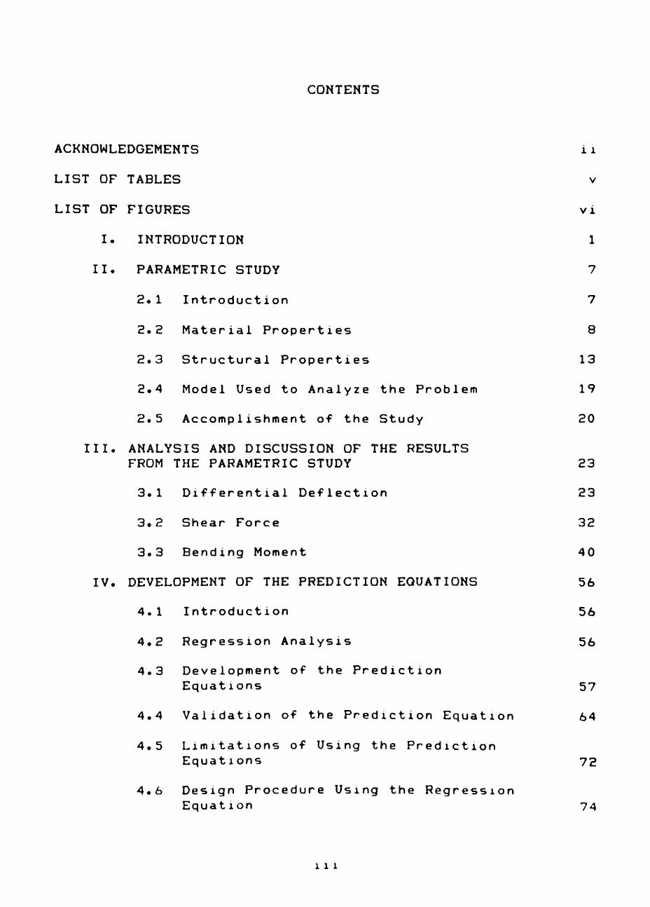
CONTENTS
ACKNOWLEDGEMENTS 11
LIST OF TABLES v
LIST OF FIGURES vi
I. INTRODUCTION 1
II. PARAMETRIC STUDY 7
2.1 Introduction 7
2.2 Material Properties 8
2.3 Structural Properties 13
2.4 Model Used to Analyze the Problem 19
2.5 Accomplishment of the Study 20
III. ANALYSIS AND DISCUSSION OF THE RESULTS
FROM THE PARAMETRIC STUDY 23
3.1 Differential Deflection 23
3.2 Shear Force 32
3.3 Bending Moment 40
IV. DEVELOPMENT OF THE PREDICTION EQUATIONS 56
4.1 Introduction 56
4.2 Regression Analysis 56
4.3 Development of the Prediction
Equations 57 4.4 Validation of the Prediction Equation 64
4.5 Limitations of Using the Prediction Equations 72
4.6 Design Procedure Using the Regression Equation 74
1 1 1

V. CONCLUSIONS AND RECOMMENDATIONS 83
5.1 Conclusions 83
5.2 Recommendations 84
REFERENCES 8 5
APPENDICES
A. MAXIMUM BENDING MOMENT, SHEAR FORCE ANE DIFFERENTIAL DEFLECTION RESULTS FROM THE PARAMETRIC STUDY 88
B. PLOTS OF MAXIMUM DIFFERENTIAL DEFLECTION 100
C. PLOTS OF MAXIMUM SHEAR FORCES 107
D. PLOTS OF MAXIMUM BENDING MOMENTS 113
E. EXAMPLE PROBLEM 121
IV

LIST OF TABLES
2.1 VALUES OF PARAMETER USED IN THE PARAMETRIC STUDY 22
4.1 COMPARISON OF R^ VALUES FOR THE THREE LOADING CONDITIONS 60
4.2 COMPARISON OF MAXIMUM BENDING MOMENT RESULTS BETWEEN THE PTI DESIGN METHOD AND THE DEVELOPED EQUATIONS IN THIS STUDY, WHEN PARTITION LOADS ARE PLACED IN X-DIRECTION 76
4.3 COMPARISON OF MAXIMUM BENDING MOMENT RESULTS BETWEEN THE PTI DESIGN METHOD AND THE DEVELOPED EQUATIONS IN THIS STUDY, WHEN PARTITION LOADS ARE PLACED IN Y-DIRECTION 77
4.4 COMPARISON OF MAXIMUM SHEAR FORCE RESULTS BETWEEN THE PTI DESIGN METHOD AND THE DEVELOPED EQUATIONS IN THIS STUDY, WHEN PARTITION LOADS ARE PLACED IN X-DIRECTION 78
4.5 COMPARISON OF MAXIMUM SHEAR FORCE RESULTS BETWEEN THE PTI DESIGN METHOD AND THE DEVELOPED EQUATIONS IN THIS STUDY, WHEN PARTITION LOADS ARE PLACED IN Y-DIRECTION 79
4.6 COMPARISON OF MAXIMUM DIFFERENTIAL DEFLECTION RESULTS BETWEEN THE PTI DESIGN METHOD AND THE DEVELOPED EQUATIONS IN THIS STUDY, WHEN PARTITION LOADS ARE PLACED IN X-DIRECTION 80
4.7 COMPARISON OF MAXIMUM DIFFERENTIAL DEFLECTION RESULTS BETWEEN THE PTI DESIGN METHOD AND THE DEVELOPED EQUATIONS IN THIS STUDY, WHEN PARTITION LOADS ARE PLACED IN Y-DIRECTION 81

LIST OF FIGURES
1.1 DISTORTION MODES 2
1.2 KNOWN DESIGN METHODS FOR SLABS-ON-GROUND CWRAY, 19783 4
2.1 EFFECT OF MOUND EXPONENT, n, AND EDGE PENETRATION DISTANCE, e, ON THE SHAPE OF THE SWELLING SOIL PROFILE CAFTER WASHUSHEN (15)] 12
2.2 EXPONENTIAL PROFILE FOR CENTER HEAVE WITH FINITE ELEMENT GRIDES 14
2.3 COMBINATIONS OF PARTITION AND PERIMETER LOADS USED FOR THE PARAMETRIC STUDY 18
3.1 MAXIMUM DIFFERENTIAL DEFLECTION OCCURRING AS A RESULT OF PERIMETER AND PARTITION (X-DIRECTION) LOAD, FOR CENTER LIFT CONDITION (P =600 LB/FT, P. =1000 LB/FT) ^ 24 iX
3.2 MAXIMUM DIFFERENTIAL DEFLECTION OCCURRING AS A RESULT OF PERIMETER AND PARTITION LOAD,(P =600 LB/FT, P.=1000 LB/FT) FOR CENTER LIFT CONBITION 26
1
3.3 MAXIMUM DIFFERENTIAL DEFLECTION OCCURRING AS A RESULT OF PERIMETER AND PARTITION (X-DIRECTION) LOAD, FOR CENTER LIFT CONDITION (P =1000 LB/FT, SLAB SIZE 48 X 24 FT) ^^ 28
3.4 MAXIMUM DIFFERENTIAL DEFLECTION OCCURRING AS A RESULT OF PERIMETER AND PARTITION LOAD (P =600 LB/FT, P. =1000 LB/FT), FOR CENTER LIFT ^ C0NDITI0i^(SLAB SIZE 48 X 24 FT) 30
3.5 TYPICAL RELATION BETWEEN EDGE MOISTURE VARIATION DISTANCE AND RELATIVE DEFLECTION FOR CENTER LIFT CONDITION 31
3.6 CONTOUR LINES SHOWING RELATIVE DEFLECTION OF THE SLAB SURFACE WHEN PARTITION LOADS ARE PLACED ALONG X-DIRECTION WITH PERIMETER LOAD, FOR CENTER LIFT CONDITION 33
3.7 CONTOUR LINES SHOWING RELATIVE DEFLECTION OF THE SLAB SURFACE WHEN PARTITION LOADS ARE PLACED ALONG Y-DIRECTION WITH PERIMETER LOAD, FOR CENTER LIFT CONDITION 34
VI

3.8 MAXIMUM SHEAR FORCES OCCURRING AS A RESULT OF PERIMETER AND PARTITION (X-DIRECTION) LOAD FOR CENTER LIFT CONDITION (P =600 LB/FT, P =1000 LB/FT) ^ 35 IX
3.9 MAXIMUM SHEAR FORCES OCCURRING AS A RESULT OF PERIMETER AND PARTITION (X-DIRECTION) LOAD FOR CENTER LIFT CONDITION (P = 1000 LB/FT, SLAB SIZE 48 x 24 FT) ^^ 37
3.10 MAXIMUM SHEAR FORCES OCCURRING AS A RESULT OF PERIMETER AND PARTITION (P =600 LB/FT, P. =1000 LB/FT) LOAD FOR CENTER LIFT C6SDITI0N (SLAB SIZE 48 x 24 FT) 39
3.11 TYPICAL VARIATION OF MOMENT ALONG THE LONGITUDINAL AND TRANSVERSE AXES WHEN PARTITION LOAD IS PLACED ALONG X-AXIS WITH PERIMETER LOAD 4 1
3.12 TYPICAL VARIATION OF MOMENT ALONG THE LONGITUDINAL AND TRANSVERSEe AXES WHEN PARTITION LOAD IS PLACED ALONG Y-AXIS WITH PERIMETER LOAD 42
3.13 MAXIMUM NEGATIVE MOMENT OCCURRING AS A RESULT OF PERIMETER AND PARTITION (X-DIRECTION) LOAD FOR CENTER LIFT CONDITION (P = 1000 LB/FT, SLAB SIZE 48 x 24 FT) ^^ 44
3.14 MAXIMUM NEGATIVE MOMENT OCCURRING AS A RESULT OF PERIMETER AND PARTITION (X-DIRECTION) LOAD FOR CENTER LIFT CONDITION (P =600 LB/FT, P. =1000 LB/FT) ^ 46 IX
3.15 MAXIMUM NEGATIVE MOMENT OCCURRING AS A RESULT OF PERIMETER AND PARTITION LOAD (P =600 LB/FT, P =1000 LB/FT) FOR CENTER LIFT^CONDITION (^CAB SIZE 48 X 24 FT) 48
3.16 TYPICAL VARIATION OF MOMENT ALONG X-DIRECTION WITH AN INCREASE IN SLAB LENGTH, WHEN PARTITION LOADS ARE PLACED ALONG X-DIRECTION WITH PERIMETER LOAD 49
3.17 TYPICAL VARIATION OF MOMENT ALONG X-DIRECTION WITH AN INCREASE IN SLAB LENGTH, WHEN PARTITION LOADS ARE PLACED ALONG X-DIRECTION WITH PERIMETER LOAD 50
V 1 1

3.18 TYPICAL DISTRIBUTION OF BENDING MOMENT IN THE LONG DIRECTION OVER THE SURFACE OF THE SLAB WHEN PARTITION LOADS ARE PLACED IN THE X-DIRECTION FOR CENTER LIFT CONDITION 52
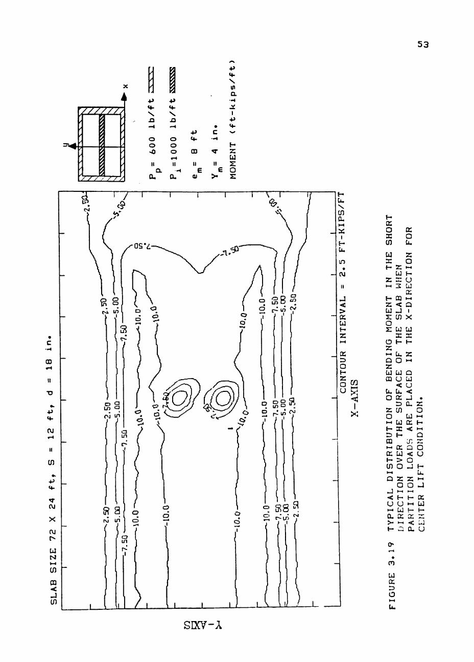
3.19 TYPICAL DISTRIBUTION OF BENDING MOMENT IN THE SHORT DIRECTION OVER THE SURFACE OF THE SLAB WHEN PARTITION LOADS ARE PLACED IN THE X-DIRECTION FOR CENTER LIFT CONDITION 53
3.20 TYPICAL DISTRIBUTION OF BENDING MOMENT IN THE LONG DIRECTION OVER THE SURFACE OF THE SLAB WHEN PARTITION LOADS ARE PLACED IN THE Y-DIRECTION FOR CENTER LIFT CONDITION 54
3.21 TYPICAL DISTRIBUTION OF BENDING MOMENT IN THE SHORT DIRECTION OVER THE SURFACE OF THE SLAB WHEN PARTITION LOADS ARE PLACED IN THE Y-DIRECTION FOR CENTER LIFT CONDITION 55
4.1 COMPARISON BETWEEN COMPUTER ANALYSIS AND REGRESSION EQUATION FOR MAXIMUM DIFFERENTIAL DEFLECTION IN X-DIRECTION 66
4.2 COMPARISON BETWEEN COMPUTER ANALYSIS AND REGRESSION EQUATION FOR MAXIMUM DIFFERENTIAL DEFLECTION IN Y-DIRECTION 67
4.3 COMPARISON BETWEEN COMPUTER ANALYSIS AND REGRESSION EQUATION FOR MAXIMUM BENDING MOMENT IN X-DIRECTION 68
4.4 COMPARISON BETWEEN COMPUTER ANALYSIS AND REGRESSION EQUATION FOR MAXIMUM BENDING MOMENT IN Y-DIRECTION 69
4.5 COMPARISON BETWEEN COMPUTER ANALYSIS AND REGRESSION EQUATION FOR MAXIMUM SHEAR FORCES IN X-DIRECTION 70
4.6 COMPARISON BETWEEN COMPUTER ANALYSIS AND REGRESSION EQUATION FOR MAXIMUM SHEAR FORCES IN Y-DIRECTION 7 1
B.1 MAXIMUM DIFFERENTIAL DEFLECTION OCCURRING AS A RESULT OF PERIMETER AND PARTITION (Y-DIRECTION) LOAD, FOR CENTER LIFT CONDITION (P =600 LB/FT, P =1000 LB/FT) ^ 101
V 1 1 1

B.2 MAXIMUM DIFFERENTIAL DEFLECTION OCCURRING AS A RESULT OF PERIMETER AND PARTITION (Y-DIRECTION) LOAD, FOR CENTER LIFT CONDITION (P =1000 LB/FT, SLAB SIZE 48 X 24 FT) ^^ 103
B.3 MAXIMUM DIFFERENTIAL DEFLECTION OCCURRING AS A RESULT OF PERIMETER AND PARTITION LOAD (P =600 LB/FT, P. =1000 LB/FT), FOR CENTER LIFT ^ C0NDITI0ft^(SLAB SIZE 48 X 24 FT) 105
B.4 TYPICAL RELATION BETWEEN SLAB LENGTH AND RELATIVE DEFLECTION OF SLAB SURFACE FOR CENTER LIFT CONDITION 106
C.1 MAXIMUM SHEAR FORCES OCCURRING AS A RESULT OF PERIMETER AND PARTITION (Y-DIRECTION) LOAD FOR CENTER LIFT CONDITION (P =600 LB/FT, P. =1000 LB/FT) P 108
C.2 MAXIMUM SHEAR FORCES OCCURRING AS A RESULT OF PERIMETER AND PARTITION (X-DIRECTION) LOAD FOR CENTER LIFT CONDITION (P = 1000 LB/FT, SLAB SIZE 48 x 24 FT) ^ 110
C.3 MAXIMUM SHEAR FORCES OCCURRING AS A RESULT OF PERIMETER AND PARTITION LOAD (P =600 lb/ft, P. =1000 LB/FT) FOR CENTER LIFT^CONDITION (iilAB SIZE 48 X 24 FT) 112
D.1 TYPICAL VARIATION OF MOMENT ALONG THE LONGITUDINAL AND TRANSVERSE AXES WHEN PARTITION LOAD IS PLACED ALONG X-AXIS WITHOUT PERIMETER LOAD 114
D.2 TYPICAL VARIATION OF MOMENT ALONG THE LONGITUDINAL AND TRANSVERSE AXES WHEN PARTITION LOAD IS PLACED ALONG Y-AXIS WITHOUT PERIMETER LOAD 115
D.3 MAXIMUM NEGATIVE MOMENT OCCURRING AS A RESULT OF PERIMETER AND PARTITION (Y-DIRECTION) LOAD FOR CENTER LIFT CONDITION (P = 1000 LB/FT, SLAB SIZE 48 x 24 FT) ^^ 116
D.4 MAXIMUM NEGATIVE MOMENT OCCURRING AS A RESULT OF PERIMETER AND PARTITION (Y-DIRECTION) LOAD FOR CENTER LIFT CONDITION (P =600 LB/FT, P =1000 LB/FT) ^ 118 ly
IX

D.5 MAXIMUM NEGATIVE MOMENT OCCURRING AS A RESULT OF PERIMETER AND PARTITION LOAD (P =600 LB/FT, P: =1000 LB/FT) FOR CENTER LIFT^CONDITION (SLAB SIZE 48 x 24 FT) 120

CHAPTER I
INTRODUCTION
One of the major causes of damage to structures,
particularly light buildings and pavements, is expansive
soil. It has been estimated that annual damages due to
shrinking and swelling of soils average $9 billion and is
the second most likely natural disaster to cause economic
loss (insect damage ranks first) CJanis et al., 19833.
A potentially expansive soil becomes a problem when the
moisture content v a n e s within the soil profile. Due to
these variations, the ground surface moves upwards (swells)
as the soil moisture content increases and the ground
surface recedes (shrinks) as the soil moisture content
decreases. Two modes of heaving distortion are commonly
identified PTI, 1980. When the soil heaves beneath the
interior of the slab, it is often called center lift or
doming. When the soil heaves around the slab perimeter,
this condition is often referred to as edge lift or dishing.
These distortion modes are depicted in Fig. 1.1. During the
swelling, the soil will often generate high pressures which
can lift heavy objects unless they are restrained, e.g., 3
feet of expansive soil can generate enough pressure to lift
a 37-ton truck 2 in. CJanis, 19833. As a result of soil
movements and pressures, structures can suffer considerable
damages. Krohn and Slosson C19803 estimated that expansive

(a). CENTER LIFT
• • • • • • • • '^• .»i . Jt*ty*' l i f c i ' ' • •-*• ''-• -''• > ' ' "ii •
FIGURE i.i DISTORTION MODES

soil-related foundation damages in U.S.A totaled $900
million in 1979. Since expansive soil can cause
considerable damage to a structure, it is important to
understand the behavior of structures on slab foundations
constructed over expansive soil.
Prior to 1930, wood frame structures supported on piers
and beam foundations were common. Since the structures were
more flexible than brick or concrete, the movements in the
building caused by the shrinking or swelling soil were not
noticed as a problem. As brick exteriors and concrete
slabs-on-ground became more widely used, the structures
became more brittle and the movements in the soil caused
considerable damage in the structures. It is believed that
many problems caused by swelling were erroneously diagnosed
as being due to settlement during this time.
The use of concrete slab-on-ground foundation became
quite common in the early 1950's, with the design
established by trial-and-error and experience CPTI, 19803.
Various design procedures have evolved over the succeeding
years for slab-on-ground foundations in residential and
light commercial buildings CBRAB, 1968; Eraser & Wardle,
1975; Lytton, 1973; Walsh, 19743. Fig. 1.2 shows the
available design procedures for slabs-on-ground over
expansive soil CWray, 19783. According to Wray, of all the
procedures listed in Fig. 1.2, "only BRAB, Lytton, Walsh
and Eraser and Wardie's procedures appears to be based
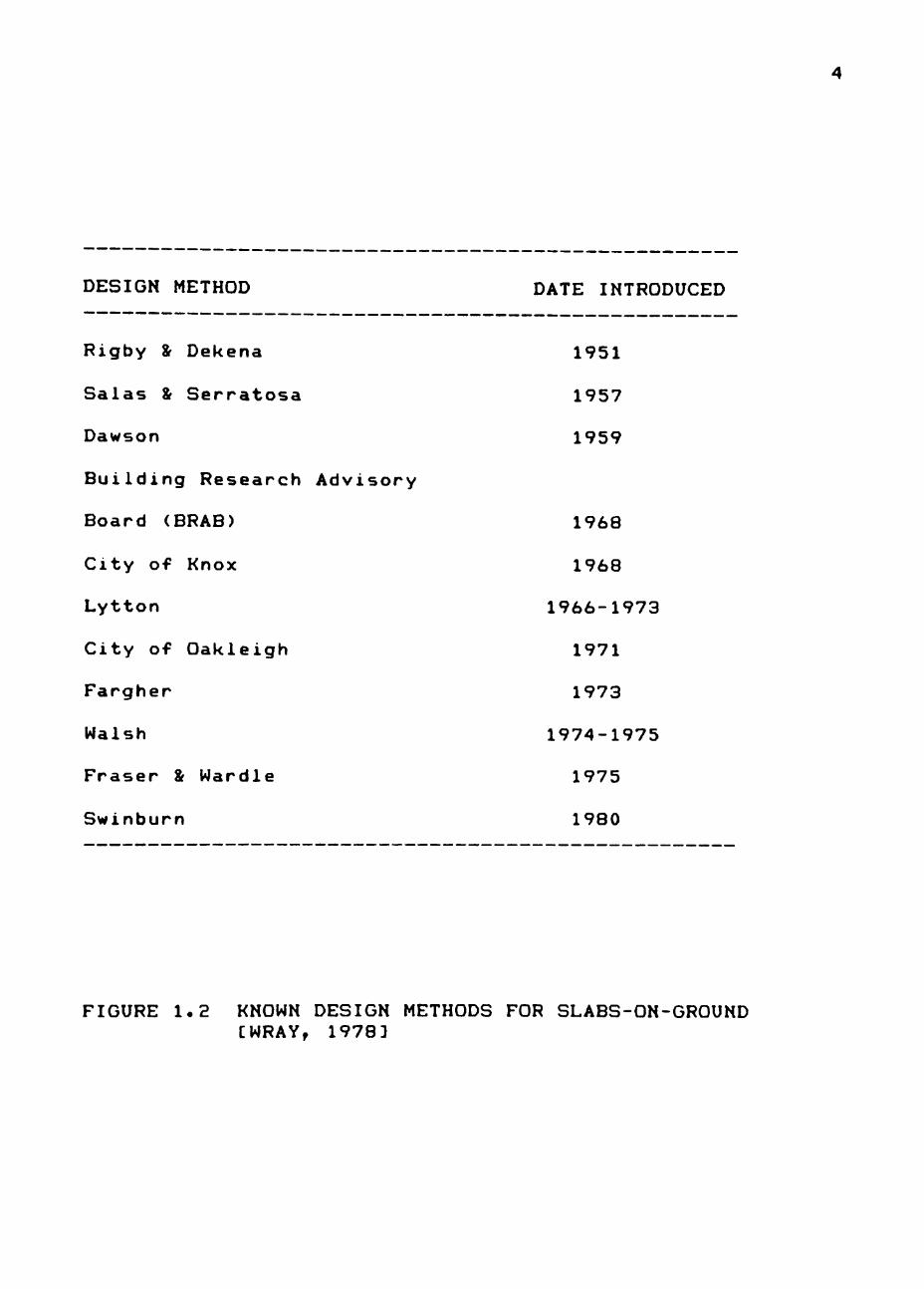
DESIGN METHOD DATE INTRODUCED
Rigby & Dekena 1951
Salas & Serratosa 1957
Dawson 1959
Building Research Advisory
Board (BRAB) 1968
City of Knox 1968
Lytton 1966-1973
City of Oakieigh 1971
Fargher 1973
Walsh 1974-1975
Eraser & Wardle 1975
Swinburn 1980
FIGURE 1.2 KNOWN DESIGN METHODS FOR SLABS-ON-GROUND [WRAY, 19783

on rational procedure and can be applied for general use."
A brief description of all the procedures is presented in
CWray, 19783. Wray, in 1978-1980, presented an analysis
that subsequently became known as the Post-Tensioning
Institute (PTI) method CPTI, 19803 for designing slabs-on-
ground. Most of the above procedures have been developed
for specific application or for certain types of problems.
Whenever a slab-on-ground is constructed for a
residential or light commercial building, the load is
usually transferred to the slab through load bearing walls
or columns at the perimeter of the slab. If a load-bearing
partition wall is supported on the slab, then a stiffening
beam is usually provided in the foundation directly under
the load or, if the load is very heavy, a separate
foundation is provided. None of the present methods of slab
design (presented above) take into consideration any kind of
line load (load bearing wail) or point load (column load) on
the interior of the slab without a stiffening beam or a
special foundation under the load. Wray [19783 studied the
behavior pattern of slabs for different perimeter loads
using different differential soil swell and edge moisture
var la tion distance. There has not been any general
com prehensive study reported in the technical literature of
the behavior of a slab constructed over expansive soils
supporting interior partition or column loads.

This study is aimed at observing how a slab constructed
over expansive soil behaves under a combination of interior
line loads (partition loads) and perimeter line loads only.
Point load (column load) is not considered in this study.
This study was designed to accomplish a parametric
investigation by taking into consideration the parameters
which influence the bending moment, shear force and
deflection occurring in the slab as a result of these loads.
From the results of the parametric study, some empirical
equations were developed from which the maximum service
moment, shear force and differential deflection of the slab
under service conditions can be predicted which then can be
applied in the design of the slab.
The next chapter describes the parameters which are
used for this study and their influence on the behavior and
performance of a slab-on-ground constructed over expansive
soil. Discussion and analysis of the results from the
parametric study are presented in Chapter III. In Chapter
IV the prediction equations are developed and discussed, and
finally conclusions and recommendations regarding further
study are discussed in Chapter V.

CHAPTER II
PARAMETRIC STUDY
2.1 Introduction
There are eight major design parameters which need to
be considered for slab-on-ground design problems, of which
three of them are soil properties? swelling mode, edge
moisture variation distance and differential soil movement.
The other five are structural properties? slab length, beam
spacing, beam depth, beam width and loading. The structural
and material parameters which are considered for this study
can be broadly classified into the following two categories?
1. Material properties,
a. Modulus of elasticity of concrete,
b. Poisson's ratio of concrete,
c. Modulus of elasticity of soil,
d. Poisson's ratio of soil,
e. Edge moisture variation distance,
f. Differential soil movement.
2. Structural properties,
a. Slab length,
b. Slab width,
c. Slab thickness,
d. Beam spacing,
e. Beam depth,
f. Loadings.

8
In this study four material properties modulus of
elasticity and Poisson's ratio of both soil and concrete are
kept constant. The properties which are used for this study
are discussed briefly.
2.2 Material Properties
2.2.1 Modulus of elastic ity of concrete. The value of
the modulus is one of the parameters which is kept constant.
The American Concrete Institute (ACI) code [Building Code
Requirements for Reinforced Concrete, ACI 318-833 gives the
following formula to estimate the modulus of elasticity for
normal weight concrete.
(2. 1 ) E =57000 ^f^~' , psi c *' c
f ' = compressive strength of concrete c
For general construction, f ' is taken conservatively as
2500 psi. Using this value in Eq. (2.1) yields a value of
E of 2,850,000 psi. Concrete is sensitive to creep and c
shrinkage. Although shrinkage occurs in the early part of
the life of concrete and is independent of the load. Creep,
on the other hand, is the property of the material by which
it continues to deform over a considerable period in
response to constant stress or load. The average long term
creep modulus of elasticity for concrete is taken as E /2
CWray, 19783. In this study a value of 1.5 X 10 psi for
E IS considered, because this value was used to develop c
the PTI equations.

2.2.2 Poisson 's ratio of concrete. Poisson's ratio is
defined as the ratio of the lateral strain to longitudinal
strain of the material. The typical range of Poisson's
ratio of concrete is 0.15 to 0.20 [Pierce, 19683. A value
of 0.15 is used in this study.
2* 2.3 Poisson's ratio of the soil. The range of the
Poisson's ratio of the soil is from .15 to .50 [Terzaghi and
Peck, 19483. For saturated soils it approaches 0.5 and as
soil becomes drier it reduces. For partially saturated soil
the value of the Poisson's ratio would be between 0.15 to
0.5. Because in this study the condition of the soil will
be a partially saturated soil and the magnitude of soil
deflections are not highly sensitive to changes to Poisson's
ratio [Gunalan, 19863, a value of 0.4 is assumed and held
constant in this study.
2.2.4 Modulus of elasticity of soi1. The modulus of
elasticity of soil is defined as the ratio of stress
variation to strain variation. The range of E varies
widely? 50 psi to 2,000,000 psi [Bowles, 1968; Gunalan,
19863.A value of 1500 psi is choosen for this study, because
this number was used by Wray, 1978 to develop the PTI
equat ions.
2.2.5 Edge moisture varlation distance (e ). It is
defined as the distance measured inward from the edge of the
slab over which the moisture content varies CPTI, 19803.

10
The magnitude of the moisture content variation largely
depends on the climate. The edge moisture variation
distance is one of the most difficult parameters to estimate
CWray, 19783. Different investigators have reported
different values of e . According to deBruijn (1975) and
Washushen (1977), the edge moisture variation distance
ranges between 2 to 5 ft. Presently, the methods of
estimating e can be broadly categorized in three ways?
(a) Experience? This method depends upon accurate
local information and upon the experience of the local
engineer. Since the climate varies from place to place, the
experience usually cannot be transferred.
(b) Estimated e from climatic patterns? This method m *^
is the most flexible method for estimating the e • Wray m
(1978) and PTI (1980) suggested that e can be approximated m
from a relationship between Thornthwaite Moisture Index and
edge moisture variation distance. The Building Research
Advisory Board (1968) has a method to estimate e from a ^ m
correlation of plasticity index and a climatic rating.
(c) Estimated with soil swelling experiments [Holland,
et al., 19803? This is an empirical method of determining
e from free and confined swelling tests, performed in an m
oedometer.
According to Wray (1978), if the range of the expected
e is considered to be between 2 to 8 ft, then most design m

11
situations will be included. On the above basis, three
values of e 2, 5 and 8 ft were considered in this study, m '
2.2.6 Differential soi1 movement (y ). If the soil L ^
beneath the slab swells uniformly, there would not be any
distortion in the slab and, consequently none in the
supported superstructure. Distortion in the slab occurs
when the soil swells non-uniformly or differentially. Thus,
the differential soil movement is more important than the
total movement of the soil. The differential movement of
the soil depends on the soil profile (stratigraphy), the
type and amount of clay in the soil, the rate of the
moisture evaporation, the depth of the seasonal movement of
moisture, the affinity of the soils for water, as well as
the climatic pattern. The shape of the swelling mound can
be expressed in terms of e and y by a simple exponential ^ m m
equation CLytton, et al., 19713,
n y = cx (2-2)
where y = an offset below the high point of the
mound.
X = the horizontal distance from the high
point.
c = a constant.
n = an exponent.
The value of the mound exponent m varies between 2 and
8 with the mound high point occurring a distance e^ inward
from the edge of the slab CWray, 19783. From Fig. 2.1, it

13
EDGE PENETRATION DISTANCE, e
Long Dimension f t ;
4 8 i : 16 20
Short Dimension ft
y = cx
FIGURE 2.1 EFFECT OF MOUND EXPONENT, n, AND EDGE PENETRATION DISTANCE, e, ON THE SHAPE OF THE SWELLING SOIL PROFILE CAFTER WASHUSHEN (15) 3

13
can be seen that a mound exponent of n=2 will produce the
least support beneath the slab, increasing values of n will
increase the support of the slab. A mound exponent of n=3
will be expected to produce a conservative value of shear,
moment and differential deflection in most cases. If the
value of n is to be considered 3 and the values of e and v m ' m
are known then the gap between the slab and the soil can be
calculated as shown in Fig. 2.2? n y =cx m
Cx = e 3 m
c=y /(e ) m m
n
n
if?
and?
then?
o^* Y;=<(y /(e )")(x ) 1 mm 1
If the range of the differential swell is selected
between 1 and 4 in., then most cases of slab-on-ground
design will be included CWray, 19783. Thus, lower bound of
1 in. and an upper bound of 4 in. is selected for this
parametric study.
2.3 Structural Properties
2.3.1 Slab length and slab width. Slab length and
slab width are usually fixed by the owner or by the
functional requirements. For residential or light
commercial buildings the slab lengths usually used are in
the range of 24 to 100 ft. For this study, three slab
lengths of 48, 72 and 96 ft slab were considered. Two slab
widths of 24 and 40 ft were considered.

14
4.
FIGURE 2.2 EXPONENTIAL PROFILE FOR CENTER HEAVE WITH FINITE ELEMENT GRIDES

15
2.3.2 Slab thickness. Four inches is the minimum slab
thickness usually used for residential structures or light
commercial buildings. In this study a constant slab
thickness of 4 in. is considered.
2.3.3 Beam depth. The depth of stiffening beams is
one of the major factors and a principal design variable in
the structural design of slabs. Increasing beam depths will
increase the bending stiffness of a given slab section and
reduce the amount of differential deflection the slab will
experience under a given set of conditions. So, the beam
depths depends on the required stiffness to limit
deflection. In some geographical areas, the minimum beam
depth is governed by the frost depth of the region, i.e.,
the beam depth must extend below the frost line to firm
bearing. For this parametric study, beam depths of 18 and
30 in. are considered.
2.3.4 Beam width. The beam widths used in practice
typically range between 8 and 12 in. A width of less then 8
in. IS difficult to excavate due to equipment limitations.
In most cases the width is seldom greater then 12 in. except
when the soil has low bearing capacity or high shear
stresses exist in the foundation. For this parametric
study, a constant beam width of 10 in. is considered.
2.3.5 Beam spacing. The spacing of beams in practice
varies between 10 to 20 ft on center. Some additional beams
may be required to be placed where there is concentration of

16
heavy loads. Increasing the number of beams will increase
the stiffness of the slab. For this study the spacing of
the stiffening beams in the longitudinal directions were 12
ft on center, but in the transverse direction it was either
12 ft on center (24 ft width slab) or 20 ft on center (40 ft
width slab).
2.3.6 Loading. Present construction practices for
residential structures do not typically include load bearing
interior walls. Instead, all roof loads are transferred to
the slab or foundation through the perimeter walls. Thus,
in contemporary construction of slabs-on-ground, the
perimeter of the slab experiences the greatest portion of
the superstructure loading. But, especially in custom-built
houses or apartment buildings, interior load-bearing walls
do occur. Because no procedure for evaluating the result of
these line loads presently exists, this study is mainly
concer ned about the effect of interior wall loadings in
combination with the perimeter loadings. The number of
combinations of partition and perimeter loadings used for
this study are grouped into four cases?
1. Case A. Partition load in the x-direction
with perimeter load.
2. Case B. Partition load in the y-direction
with perimeter load.

17
3. Case C. Partition load in the y-direction
without perimeter load.
4. Case D. Partition load in the x-direction
without perimeter load.
The above combination of loadings are shown in Fig. 2.3.
Perimeter wall loads for a light structure and a heavy
two-story masonry structure might typically be found to be
600 lb/ft and 1500 lb/ft, respectively CWray, 19783. For
this study the minimum and maximum values of perimeter
loading used were also 600 lb/ft and 1500 lb/ft. For
interior wall loadings, a minimum value of 100 lb/ft, an
intermediate value of 1000 lb/ft, and a maximum value of
3000 lb/ft were considered.
In addition to the perimeter and partition loads, the
weight of the concrete slab and some additional interior
loading are also considered. The weight of the concrete
slab is calculated by the volume of the concrete in the slab
multiplied by the unit weight of the concrete which was
taken as 145 pcf. Additional loading due to plumbing and
mechanical systems, appliances and household furnishing are
also considered. However, for all these loadings, it is
difficult to know their magnitude and location. According
to the American National Standard Building Code requirements
for minimum design loads in the building and other
structures, a minimum uniformly distributed live loading of
40 psf applied over the entire slab is recommended for

18
Y
K<. <. ^^VVVV .VVVVVV-\ \
\ \
" >^^^>=«»=x>«*M^^
f Perimeter Load
A^^^^^^^VV<.^V^^^^v
^
t ^kk^^^^Vk^^^kkk^^ks^ ' ^ ' s^^^^k .kV^k '^ ' ^^Tr^ t\ Partition
Load
1. Case A, partition load in the x-direcrion with perimeter load.
NX^^V^V's^VVVVvVVV^VVV-sV^'s-s^VV-sVVs^^-W \
! L « \k\'\'\\\\\\^^^\\VVV^VVVVVVVV\\V\VVVV'b
2. Case B, partition load in tiie y-direction with perimeter load.
3. Case C, partition load in the y-direction without perimeter load.
v\\\^^\^^N\\\^\v^^^\\N^^^\\^^v\^^^^^
4. Case D, partition load in the x-direction without perimeter load.
riGUFE 2.3 COMBINATIONS OF PARTITION AND PERIMETER LOADS USED FOR THE PARAMETRIC STUDY

19
private apartments and dwellings. This 40 psf uniformly
distributed loading was also included in the computer model
used in this study.
2.4 Model Used to Analyze the Problem
This study was accomplished by employing a finite
element computer program to analyze plates resting on a
semi-infinite elastic half-space. The original computer
program was written by Huang (Jan, 1974). Huang
incorporated a scheme which makes use of the symmetry of the
slab Huang (May, 1974). The program was developed to
calculate stresses and total deflections occurring in
concrete pavements and was used to analyze pavement
thicknesses of constant section. Also, this computer code
considers situations where there is full contact between
slab and the supporting soil at all times, initially full-
contact but subsequent non-contact conditions, or initial
gaps between the slab and subgrade but full contact may
never occur. Huang (Jan, 1974) compared the results from
the computer program with field experimental measurements.
Based on these comparisons, he showed that the deflections
predicted by the program compared reasonably well with the
field results.
Wray (1978) modified the original program for analyzing
stiffened slab-on-ground foundations supported on expansive
SOI 1. The program was modified to permit the analysis of a

20
slab with stiffening beams as well as a slab of uniform
thickness. The program was also modified to calculate shear
forces. The program with the above features was named slab2
by Wray (1978).
2.5 Accomplishment of the Study
The study was conducted in three phases; (1) analysis
with partition or interior loads onlyj (2) analysis with
both perimeter and partition load in the x-directionj (3)
analysis with both perimeter load and partition load in the
y-direction. The following assumptions were made for the
study 5
1. The slab is monolothic.
2. The loading was continuous and symmetrical.
3. The slab would not be exposed to severe weather
and there would be no significant temperature differential
across the thickness.
4. The longest dimension of the slab was always
taken to be in the x-axis of the slab.
5. The slab was discretized into square
elements with an aspect ratio of 1.
With the above assumptions and the values of the
se lected parameters which have already been discussed, the
parame trie study was done in a systematic manner. For the
convenient reference, the selected parameters are summarized

21
in Table 2.1. The parametric study was accomplished by
varying the parameters listed in Table 2.1 one at a time in
a specific manner, thereby including all of the possible
combinations.
The parametric study included a total of 450 cases for
all of the conditions. The values of the several design
parameters (moments, shears, deflections) as calculated from
the computer code are included in the Appendix A. The
results of the analysis include bending moment, shear and
differential deflection over the distance (distance between
two nodes). These results are discussed in Chapter III.

22
Table 2.1. VALUES OF PARAMETER USED IN THE PARAMETERIC STUDY
Parameter Symbol Value Unit
Modulus of Elasticity of Concrete E 1,500,000 psi
c Poisson's Ratio of
V
Concrete C 0.15 a Modulus of Elasticity of Soil
Poisson's Ratio of Soil
Slab Length
Slab Width
Slab Thickness
Beam Spacing
Beam Depth
Edge Moisture Variation Distance e^ 2,5,8 in
Differential Soil
Movement Y^ It^ ^^
Perimeter Load P^ 600,1500 lb/ft
Partition Load P^ 100,1000,3000 lb/ft
a= dimenslonless
E s
V
S
L
W
h
S
d
1,500
0.40
48,72,96
24,40
4
12,20
18,30
ps
a
ft
ft
1 n
ft
1 n

CHAPTER III
ANALYSIS AND DISCUSSION OF THE RESULTS
FROM THE PARAMETRIC STUDY
The results of the parametric study include
deflections, bending moments and shear forces. The data
obtained from the parametric study are described briefly
below :
3.1 Differential Deflection
The deflection at each finite element node were
determined by the computer program and, then, the maximum
differential deflection was calculated from the individual
deflections. Data obtained m the analysis are shown in
Appendix A. The differential data is plotted as a function
of edae penetration e and slab length which are shown in ^ m
Figs. 3.1 to 3.5, and in Appendix B. The following general
observations can be made from the figures mentioned above.
1. There is little increase in differential deflection
for e =0 to 2 ft, for different slab length Fig. 3.1. m
2. There is slight increase in differential deflection
when partition loads are placed in y-direction Fig. 3.2.
3. Differential deflection increases with the increase
in perimeter load Fig. 3.3.
23

24
Ci
B
I ><;
EDCC PEHCTPA03H (FT|
(a) DIFFERENTIAL SOIL MOVEMENT (v ) = 1 ,n m A 1 n .
ui
3
1.9
i.a -
1.7 -
1.B -
1.5 -
1.4 -15 -1.3 -
1.1 H 1
D.g
D.B H
Q.7
D.B -
0.5 -
0.4 -
0.3 -
D.3
D.I H
0
d '= 18'
aAQ ft slab + 72 ft slab o 96 ft slab
CDCE PFHnPAn:>H . : [ T |
(b) DIFFERENTIAL SOIL MOVEMENT (y ) = 4 in.
r GURE 3.1 MAXIMUM DIFFERENTIAL DEFLECTION OCCURRING AS A RESULT OF PERIMETER AND PARTITION (X-DIRECTION) LOAD, FOR CENTER LIFT CONDITION (P =600 LB/FT, P =1000 LB/FT)
P IX

25
z z D
! b a =!
Ui
^ 5 s 3 2
^ 2
3
1.9
1.B
1.7 1.6
1.5
1.4 1.S
1.3
1.1
1
o.g D.B
D.7 OB
D.S
0.4
D.a 0.3
0.1
0
CODE PEHCTR>^.1>:>N (fX}
< C ) . DIFFERENTIAL SOIL MOVEMENT (y ) in
i n *
z D
[b
^
EOCE PEMETP.-.TVOH . : F T |
( d ) . DIFFERENTIAL SOIL MOVEMENT ( y ) = 4 m
i n (
FIGURE 3.1 CONTINUED

26
a
s -I
i ui
SLifi LEHCTH ( r r i
(a). DIFFERENTIAL SOIL MOVEMENT
D
n fi
e UI
I
SLifl UEHCTH \ r ( ;
( b ) . DIFFERENTIAL SOIL MOVEMENT (y ) m
= 4
FIGURE 3 . 2 MAXIMUM DIFFERENTIAL DEFLECTION OCCURRING AS A RESULT OF PERIMETER AND PARTITION LOAD, (P =600 LB/FT, P =1000 LB/FT) FOR CENTER LIPT CONDITION ^

27
D
I C I
UJ
1 9 -
1.B -
1.? -
1.B -
1.5 -
1 . 4
1.3 H
1.3 -
1.1 H
1
D.g
D.B
0.7
D B H
O.S
D.4 -
D.3 - -
0.3 i
01
0
d = 3 0 "
CH
a P. x - d i r e c t i o n + P^ Y - d i r e c t i o n
1 '
- • £ 1
4fl gB
5L-a lEHCTH \n\
( c ) . DIFFERENTIAL SOIL MOVEMENT (y ) 1 in.
z 2 n \-> ^ \h i " j
^ e lU
1 L j
zs s
1 9 -
I B -
1 7 -
I B -
1.5 -
1.4 -
1.3 -
1.3 -
1.1 -
1 -
0.9 -
n.B -
0.7 -OB -i
0.5 -
D.4 -
0.3 -
0.3 -r
n 1 -
d » 3 0 "
a P. x - d i r e c t i o n + P. v - d i r e c t i o n
1 '
. — 1
1
1
. • B — - ~ "
0 -\ 4B
( d ) .
— ,
DIFFERENTIAL SOIL MOVEMENT m
= 4 1 n«
g
FIGURE 3.^ CONTINUED

r-fc
"Z. D
\-> "^ i] C i
-4 <. e UJ
1.
u.
2 3* 2[
V _ £
2
19
I B
1.7
I B
15
1.4 1.3
1.3
1.1
1 0.9
D.B
0.7 06
OS
0.4
0.3
0.3 0.1
0
28
d = 18"
a P = 600 lb/ft PJ=1500 lb/ft
.- _—Q-
EOCE PEHETPATVOH - jT!
( a ) . DIFFERENTIAL SOIL MOVEMENT (y ) m
1 in.
\ o
g ui
i5
3
19
IB
1.7
IB
1.5
1.4
1.3
1.3
1.1
1
D.9
OB
0.7
OB
D.S
0.4
0.3
0.3
0.1
0
d = 18"
p = 600 pP=1500
lb/ft lb/ft
- - • i i
.—s"
:rz=S—-
EDCE PEHnB.'i.nC-H iFT;
(b). DIFFERENTIAL SOIL MOVEMENT (y ) m
= 4 in,
FIGURE 3.3 MAXIMUM DIFFERENTIAL DEFLECTION OCCURRING AS A RESULT OF PERIMETER AND PARTITION (X-DIRECTION) LOAD, FOR CENTER LIFT CONDITION (P =1000 LB/FT, SLAB SIZE 48 X 24 FT)
IX

29
- , , z D
f> ^ lb C I
-4
e LlJ
^ 5 3
5
' -i.
3
1 9
I B
1.7
1.6
1.5
1.4
1.3
1.3
1.1
1
0.9
OB
0.7
0.6
0 5
0.4
0 3
0.3
0.1
D
d = 30'
a P = 600 + P'' = 1500
P
lb/ft lb/ft
EJ-
EOCE PEHETPAnnH 'TT!
(c). DIFFERENTIAL SOIL MOVEMENT (y ) m
= 1 in.
_,— t^
z D
r, ^ lb C i
-4
E i j
\
" !!c
.rf_'
-
3
1.9
1.B
1.7
1.B
1 5
1.4
1.3
1.3
1.1
1 0 9
D.B
0.7 0.6
0.5
0.4
0.3
0.3
0 1
0
- d = 30"
P = 600 a + p'^slSOO
P
lb/ft lb/ft
=*---
EDCE PEHETPAnC-H i.FTI
<d). DIFFERENTIAL SOIL MOVEMENT (y ) m
= 4 1 n.
FIGURE 3.3 CONTINUED

30
D
r>
Ci
UJ
a
3
I.a H I B
1.7 -
I B -
1.5 -
1.4 -
1.3 -
1.3 -
1.1 -
1 -
O.g -
D.B
0.7
0.6 -
0.5 -
0.4
0.3 -
0.3 -
0.1
a d •». d
18" 3 0 "
— • J I
:?=—-
EDGE PEHnPAT>:>H tyVt
(a). DIFFERENTIAL SOIL MOVEMENT (y ) m
i n .
i Ci
in
I
EDCE PEHETPATK>H (fV,
( b ) . DIFFERENTIAL SOIL MOVEMENT ( y ) m
= 4 i n .
FIGURE 3 . 4 MAXIMUM DIFFERENTIAL DEFLECTION OCCURRING AS A RESULT OF PERIMETER AND PARTITION LOAD-(P =600 LB/FT, P =1000 LB/FT), FOR CENTER LIFT CONDITION (^CAB SIZE 48 X 24 FT)

31
a>
. *J <*•
'T fU
II
3
. V <•-
(VJ «-• II
C/1
. c •M
T
II
E >
4J '•-\ n ^~i
o o >0
II
a. a.
*j
<*-\ n —<
o o o II
Ou
Z H o u. H-t t-H
H J < •-• CC K LU < H > Z
U] LJ U X D K H O U) U. t-H
o z z: o >-» UJ H o u a u U J
u. Z UJ UJ Q UJ •z UJ H > UJ ^ CQ H
< Z J a UJ - . K r-< Q J Z UJ < K
UJ J U < z u < •-• H a, en •^-i »-i
•r- n
Z o hH
H HH
Q Z O u
I
in
I
(S3HDNI) N 0 I 1 0 3 1 J 3 a 3 A I l V 1 3 d

32
4. Differential deflection increases with the increase
in edge moisture variation distance Fig. 3.1.
5. The differential deflection reduces as the beam
depth increases Fig. 3.4.
6. The total deflection of the slab increases with the
increase in e Fig 3.5. m ^
The differential deflection does not always increase
with increasing e • For small y , large e and large m m m
perimeter and partition loads, the edge of the slab was
discovered to bend down until it came into contact with the
subgrade. Thus, for large values of e , there is little m
oppurtunity for the deflection to increase because the soil
is helping to support the edge of the slab.
The distribution of deflection on the surface of the
slab is shown in the Figs. 3.6 to 3.7. The maximum
deflection of the slab occurs near the edge of the slab
irrespective of the position of the partition load. Fig.
B.4, shows the typical relationship between slab length and
deflection of the slab under perimeter and partition load.
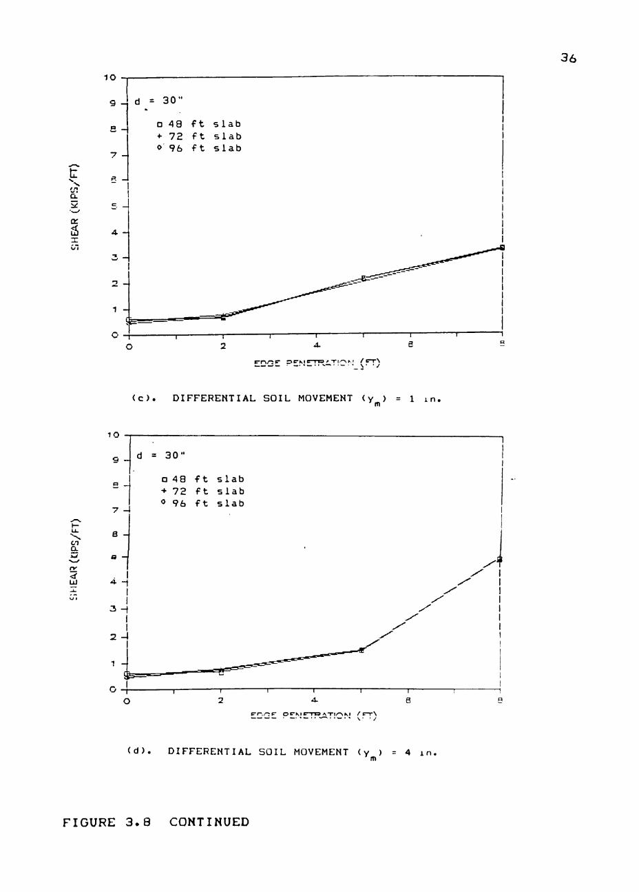
3.2 Shear Force
The shear force data obtained from the analyses are
shown in Appendix A. The values of shear force are plotted
as a function of edge penetration distance in Figs. 3.8 to 3
10, and in Appendix C. From the figures and Appendices the
following observation can be made.

rxi
X
vy//.y''i / / /
!
:zz
* c
II
/
-p ^
CD
II £
(U
4J M-\ JD — <
O O 0
II a
cu
4-> *4-\ X3 -H
o o o
It
D,
33
c
-j_.L_j_iL_/2l^^:
-
.H
• o
II
J <; >
cx UJ H Z »-«
a D O H Z o u
0] A
XI
1 ^^
o z UJ O H
X J u. H < •H
-J U, Q O UJ CC
U UJ Z < H O J z t-. Q. UJ H U U UJ UJ cc cx -3 «3: o U- u. UJ en Q Q ..
< Q UJ o < > J o ^ J H Z < o cx J »-• UJ UJ H H cx (- UJ
o cx •-• z < cx •-• 0, UJ 2 Q,
o z Z UJ z en z H 2 •-.
en 3 UJ UJ
z u z »-' < O ' -J u, •-< 2:
cx H C cx : u •-• ::3 en uj H o cx •-< H 03 >-i G z < Q r: G ^ 1 3 u en X .
>0
n UJ cx => o
^

=J)
c
II
4-
II
O O
CL
34
4^ "4-\ J3
O O O «H
II
a,'
o z
UJ o Z J H <
u, o z o
Q UJ
u <
cu
U UJ UJ cx J < u, UJ en
u.
cx Ci]
Z UJ
u o U,
Q < o -1
cx
UI
Ul
cx UJ cx z
z O '
J Lu •-• Z
Q
UJ >
H <
UJ f-cx »-•
O CX z <
Q < O
z o
2 O z en
z UJ z 2
en UJ UJ
u < u, cx en
cx
o
z o u en
CD <:
u UJ cx »—( Q I
a z o u
UJ
cx
o
srxv-A

35
a.
X (/I
- -1
e -
d = 18"
• 48 ft slab + 72 ft slab « 96 ft slab
E D G E ! OC-MC-rTSATf /^M / P T ^ W W W. , W . . V-,. , w . . y. , J
<a). DIFFERENTIAL SOIL MOVEMENT <y ) = 1 i n *
Q .
CU <i UJ X C/I
9 -
5 -
4. -
3 -
d = 1 8 "
^ - r -o
• 4 8 f t s l a b + 7 2 f t s l a b o 9 6 f t s l a b
EDGE PENETRATION (FT)
( b ) . DIFFERENTIAL SOIL MOVEMENT (y ) = 4 ^ p .
FIGURE 3.8 MAXIMUM SHEAR FORCES OCCURRING AS A RESULT OF PERIMETER AND PARTITION (X-DIRECTION) LOAD FOR CENTER LIFT CONDITION (P =600 LB/FT, P =1000 LB/FT) ^ IX
36
«/ • C L
CE
X
10
9 _ d = 30"
p _
y -
p, _i
D 48 + 72 o 96
ft slab ft slab ft slab
T _
1 5E==
O -r -I 1 r -2 A. e
(c). DIFFERENTIAL SOIL MOVEMENT (y ) = 1 in. tti
en Q.
o;
LU
C-f./^C- O C - M A T I / ^ M ('I
(d). DIFFERENTIAL SOIL MOVEMENT (y ) = 4 in. m
FIGURE 3.8 CONTINUED

37
tr
X 0-
a
X on
<3 _
H _
7 -
= 1 8 "
D P = 6 0 0 l b / f t + P ^ = 1 5 0 0 l b / f t
w - T -O
- T -2
-r-A.
^DGE PENETHATION ''FT'^
B
< a ) . DIFFERENTIAL SOIL MOVEMENT (y ) = i m .
10
D P = 6 0 0 l b / f t + P ? = 1 5 0 0 l b / f t
EDGE PENETTRATiON (FT )
( b ) . DIFFERENTIAL SOIL MOVEMENT (y ) = 4 i n . 01
-1
a
FIGURE 3.9 MAXIMUM SHEAR FORCES OCCURRING AS A RESULT OF PERIMETER AND PARTITION (X-DIRECTION) LOAD FOR CENTER LIFT CONDITION (P^^=1000 LB/FT, SLAB SIZE 48 X 24 FT)

t CL
2i
e -
6 -
d = 30"
D P = 600'lb/ft + Pp=1500 lb/ft
1 ^
2 -r— 4.
1 ^
B - I a
EDGE PENETFUXTION (FT)
( c ) . DIFFERENTIAL SOIL MOVEMENT (y ) = 1 m . m
'Si
a
UJ
erv/^c- O C M c—rca A-ri/^K i (FT)
(d). DIFFERENTIAL SOIL MOVEMENT (y ) = 4 in.
FIGURE 3.9 CONTINUED

39
Q.
UJ
a. iA
C/1 CL
^ -
UJ X C/l
e
7 -}
6
5 -
4. -
3 -
9 -
e -
7 -
6
5 -
4. -
3 -
2 -
1 -
tB
a d = 1 8 ' .•»-_d = 3 0 -
-r.i^c- PENETRATION 'FT)
( a ) . DIFFERENTIAL SOIL MOVEMENT (y ) = 1 i n . m
a d = 18 + d = 3 0
EDGE PENETRATION (FT)
( b ) . DIFFERENTIAL SOIL MOVEMENT (y ) = 4 i n .
FIGURE 3.10 MAXIMUM SHEAR FORCES OCCURRING AS A RESULT OF PERIMETER AND PARTITION LOAD (P =600 LB/FT, P =1000 LB/FT) FOR CENTER LIFT^CONDITION (i^AB SIZE 48 X 24 FT)

40
1. Shear force does not vary with an increase in slab
length Fig. 3.8.
2. Shear force increases with an increase in perimeter
and partition load Fig. 3.9.
3. The shear force almost remains the same
irrespective of the direction of the partition or line load
( X or y direction) Appendix A.
4. Shear force increases with an increase in beam
depth Fig. 3.10.
3.3 Bending Moment
The magnitude of negative and positive moments shows a
similarity of variations along the longitudinal and
tranverse axes whether the loads consist of partition,
perimeter or a combination of both placed along the
transverse or longitudinal axes. Variation of the moments
along the longitudinal and transverse axes for a slab size
of 72 X 24 ft in Figs. 3.11 to 3.12, and also in Appendix D.
From these figures the following observation can be noted?
1. The moment profile along the longitudinal
and transverse axes differ considerably. When loads are
placed along the longitudinal axes, the maximum moment in
the longitudinal direction occurs near the edge of the
slab, whereas for transverse loading the maximum moment
occurs near the midpoint of the slab Fig. 3.11 and Fig.
3. 12.

B 41
03
. c
• H
«-«
II £
>'
V «•-
CVI
II E
OJ
-P <•-\ J3 —H
o o O
II
a CU
+J «*-\ XI - H
o o o II
•- a.
J < Q Z LJ •-• U Q < D J f- a. h-(
o cn Z t-i
c J Q <
u o I -J H
•"TT-
—« o o z •-• C t ->J I-" < • -
•-v »A«
H < z a. LJ ~, .
3 u: •rr "T"
• 7
U, 3 X
Ui Z X c < •—1
H Lu < X <— X X Lu <: > > J)
•^ — < < X
• .--s
< ..
- y
•-J r--^ -
1 — 1
' • V
fc—«
•- !— — < 2
cn »- X < 1
X
i- < <
IJj/SJI'1-iJ I I]ij..u»'J

H 42
y / / / / ^ .
r *
1 H : \ U c * -^ ^y/^yy^/y/// i ^ ^ H
: \ n .. 03 T - t
1 " 1
-A ^ V->
-p -p C 4 . ^ -
:~s ru II II -J 2
1
I t
1
1
1 J r 1
t 1
"
. ^
1
n
b
b
'
J ^ 7 ^ 7~f
E
— B - — " ——~"
-* ——««. ~ ~ — f i - — _
1 1 1 1 1
'iT' •+ C J -r- Oil ^i"l
' - ' - ' - O Cl
1 u/\
• p
CVJ
II E
01
___—
""—-__
1
-h
iD
:dn-
-p +*
£i n — —<
o o o o vO o
«-• II II
a -t a. a.
^ ^ . . - • • "
[ J — _ ^ _
—a . - - ^
.-•Q" ' , - B " '
P'
— - 4 3
• _--— • ....-t---
a ' ..A--"
-3- I . ' -- U "
,' '.
4,
--a. ' "-h...
- P "••-+-.. . .__
^ ' • + * - - .
[J] ____J::--- f - — T T - "
cn U-J
u -^ ! ''"'"' j
i ^ i a '
1
a. ! ' " & • - . 1
• " • • a - - . !
"""-Q i
_ — — a rk — . ^ Lp
1
1
1 1 1 1 i 1
CJ O (J -+ 'V OD ^ Ci
O O Cl Cl i~ ' <—
: 1 1 1 1
- ^ ' U f ' J jM'L^J
z u Q < D J t - QL t—1
o cn z •-• o
< LJ C Z J
z —• c G f- <: - ] ^ c <; H _j
t _
f- < a: z a. j j UJ ^ z z u: G JJ SI 21 Z »-i
2 ^ a. 'Xi G CD a.
4^^ ^ J ^
G < H >—< • — (
H W Z
-- a: cn a : CJJ • -< > X > 'S) <
Z 1 - : < >-< a: U H o — z >• Z -J .- < <
ai
.
m LJ a: D
o x

43
2. When partition loads are placed along the
transverse axes without perimeter load, the magnitude of the
transverse and longitudinal moments both peak near the
center of the slab (Fig. D.4).
3. From Figs. 3.12 and D.4 it can be concluded
that when perimeter loads are added along with partition
load, the magnitude of the negative bending moment increases
both in the longitudinal and transverse axes.
The maximum negative moment is plotted as a function of
edge moisture variation distance and the moment variation is
plotted with varying slab size which are shown in the Figs.
3.13 to 3.15, and also in Appendix D. From these figures
the following observations can be notedJ
4. The moment increases with increasing edge moisture
variation distance Fig. 3.13.
5. The moment does not vary with the increase in the
slab length Fig. 3.14.
6. The moment increases with the increase in perimeter
and partition load Fig. 3.13.
7. The moment increases with the increase in beam
depth Fig. 3.15.
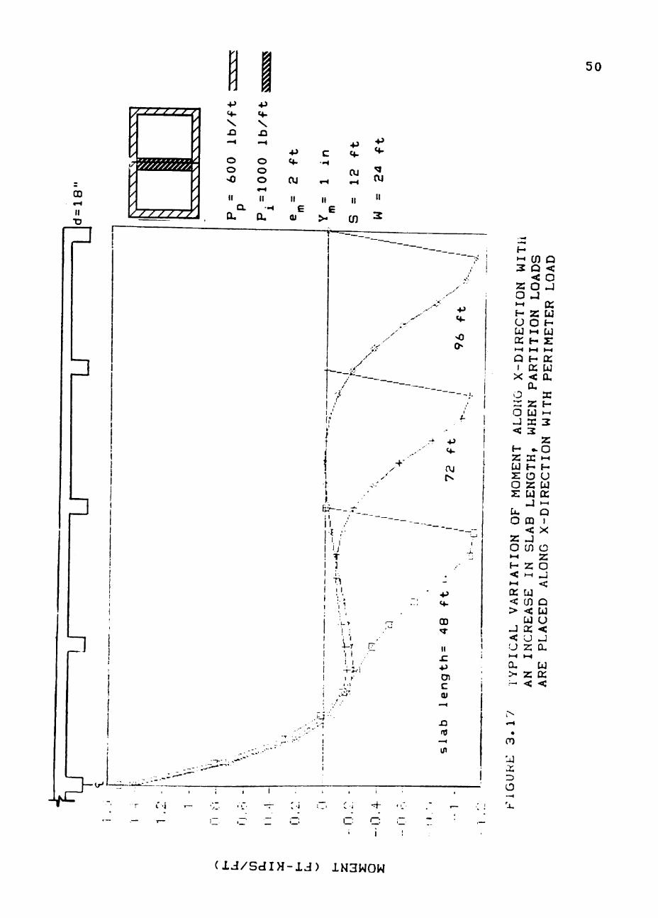
8. Multi modal bending occurs in longer slabs
irrespective of the position (longitudinal or tranverse) of
the partiton load Figs. 3.16 and 3.17.

44
t
I
UJ
^
/'i
>
20
19
16
14. -
12 -
d = 18"
D P = 600 lb/ft + P^=1500 lb/ft
2 5
EDGE: PENETTRATION (FT)
8
(a). DIFFERENTIAL SOIL MOVEMENT (y ) = 1 in, m
nn
i2
Cl' UI
>5
a P = 600 lb/ft 4- pP=1500 lb/ft
20 -I d = 18"
18
16
1J.
12
10
a
cr^nr OTKI t- I V J A T I / ^ ON (rr)
<b). DIFFERENTIAL SOIL MOVEMENT (y ) = 4 in. m
FIGURE 3.13 MAXIMUM NEGATIVE MOMENT OCCURRING AS A RESULT OF PERIMETER AND PARTITION (X-DIRECTION) LOAD, FOR CENTER LIFT CONDITION (P.^=1000 LB/FT, SLAB SIZE 48 X 24 FT) IX

45
I
LLI
1^
>:;
22
2 0
IB
16
-4 d = 3 0 "
a P = 6 0 0 ' l b / f t + P = 1 5 0 0 l b / f t
P / •
EDGE PENETRATION (FT )
( c ) . DIFFERENTIAL SOIL MOVEMENT ( y „ ) = 1 i n ,
I
1x1
^ ZJ ^ ^
19
IB
d = 3 0 "
a p = 6 0 0 l b / f t + P ^ = 1 5 0 0 l b / f t
P
EDGE PE^JETRATION (FT )
( d ) . DIFFERENTIAL SOIL MOVEMENT (y ) = 4 i n . rti
FIGURE 3.13 CONTINUED

4 6
a
I
_>
LU
^ ^
n
LU
o
EDGE PENETRATION (FT^
< a ) . DIFFERENTIAL SOIL MOVEMENT ( y ) = 1 i n , m
1 g -I
16
14. -
12 -
10
a
5
A -I
d = 18"
a4a ft slab + 72 ft slab « 96 ft slab
p-nr; PENETRATION (FT^
<b). DIFFERENTIAL SOIL MOVEMENT (y ) = 4 in. m
FIGURE 3. 14 MAXIMUM NEGATIVE MOMENT OCCURRING AS A RESULT OF PERIMETER AND PARTITION (X-DIRECTION) LOAD FOR CENTER LIFT CONDITION (P =600 LB/FT P =1000 LB/FT) ^ IX

47
u.
Q.
LJ
ft
20-1 d
15 -
16
14 -4
12 -4
= 30"
D 48 ft slab * 72 ft slab o 96 ft slab
i2
UJ
o
(c). DIFFERENTIAL SOIL MOVEMENT (y ) = 1 in. tn
EDGE PENETRATION <'FT"i
( d ) . DIFFERENTIAL SOIL MOVEMENT (y ) = 4 ^n. fti
FIGURE 3.14 CONTINUED

48
a T
ill
6
c2 t-,
LJ
•y.
o
LU
O
' -7
a d = 1 3 " 4- d = 3 0 "
e-r\/-;e" p'^^j ETRATION (FT^
(a). DIFFERENTIAL SOIL MOVEMENT (y ) = 1 m .
EDGE PENETRATION (FT)
( b ) . D I F F E R E N T I A L S O I L MOVEMENT ( y ) = 4 i n . n)
FIGURE 3.15 MAXIMUM NEGATIVE MOMENT OCCURRING AS A RESULT )F PERIMETER AND PARTITION LOAD (P =600 LB/FT, P =1000 LB/FT) FOR CENTER ElFT C0NDITI0A^(SLAB SIZE 48 X 24 FT)

i 49
00
« "Do
•p ^ •
\ £i • H
o o >0
II Q.
QU
4J <•-\ n -^
o o o II
• - ^
CL
4 i <4-
CVI
II E
(U
c • - <
• H
11 E
>
4J «•-
OJ •-•
II
cn
4J «•-
^ lU
II
^
1—«
2
Z o • H
H u u V 1 — ^
• -«
Q 1
X
o '-r'
o -J <
I—• -r-
^ . £ .
o z J - l
o z o •-( H <: HH
K < >
J < u t-H
Qu >• (—,
U) a < < o o J
z o H-»
H t—t
H CC < CL
Z UJ Z 3
*. z H O z u -3
CQ < J 0)
z t-H
u cn < Ui cc u z t-t
z <
J
o: U] H u "^ 1 ^
ct; u Qu
Z H •—» 3
Z o t—«
H u u hH
Q 1
X
o ^-r'
O J <
a u u < J QU
U Q: <
. cn u a: O
iJJ . ' ' 'Sd l ; i -U ) lf'G^'^L4'J
/ J ^ / / 7 ?
/
^
'' >
<
" ^ ^ 1
/ft
A r J -D J3
CD
'• i •D
^
1
; ' • m» ^ * ^ ^ * * ^ , ^ , TA ^ ^ ^ ^ H . *
/
>/ ^ ^ ? />'
>
f
1
1
1 1 ) '
P i 1 1
'
1
' 1 — LH'-
• - J - - 1
. - - : ;-;->^'^' •_,^~'~''~~
\ - • -
^ n - ^ r :. i ^ .•-
— — T — 1 .
3 o 0 o cu
1 II II a H g
I. a. (u
- • • ; ' - •
,—-*
1
*"
1
• • ' . : - • •
. " ^ ' ^ • • ' ' • "
1 :
-^ ' i I t
4i *"
II II "
~——___
_-_.*-•
P.«"
/
~ jl
/ 1 •.' ( i -
•
f i I ^-t /^ 1 •t •
f. tir—-.rL_ i l •• ~ ~ ~ ~ " - -w 1 Ij' ! T 1 ] 1 ;_ 1 T 1 I I 1 'i * ( 1 .» - 1
1 - h ^ '^
1 i ' l
1 i 1 ••' 1 4 - M 1 1 y
1 -1
! P' i '.••' ••'
.>- j " '
" • '
1 t
i i
j ;
: - :•* • + ••:•
C Q :~
4^ * * •
>0
~ " " r "
f
•-
--+ -P «•-
OJ r
U-J
1
' *i <•-
QD ^
4->
Dl c <u
- H
£1 rfl
—« in
1
1 '
r- :
- '
•^
ION WIT
LOADS
R LOAD
H Z W U O H UJ HH UJ Ci: H s ^-t t-4 >-l a f- Q: 1 cx UJ
X < a,
1 ^ 1 Z Z f-, O UJ •-H 1 J Z 2 i < 2
z H . . O z z •-• UJ H f-s: CD u O Z UJ s u cc
J ^ U. Q O OQ 1
< X Z J o cn c •-• z H z o < t-H J
QC UJ < (S) a > <: UJ
UJ u ^ X < < U J U Z Du >-* t-t a. UJ > z Q; , ^ < <
^ • ^
»-4
« m
UJ : i ; =3 o - H
J '-1.
50
( I J / S d I H - l J ) 1N3W0W

51
A plan view of the moment distribution on the surface
of the slab is shown in Figs. 3.18 to 3.21. For (1)
partition load in the x-direction with perimeter load and
(2) for partition load in the y-direction with perimeter
loadf it is observed that the maximum long direction moment
occurs near the edge of the slab and the short direction
maximum moment occurs near the center of the slab^
irrespective of the position of the partition load.
A total of 450 cases were studied. From these problems
only the absolute maximum values of differential
deflection^ bending moment and shear force were used for
the regression analysis. The regression analysis is
discussed in Chapter IV.

52
H U. \ cn a. t-t
:/: 1
H U.
in .
(U
n
J < > OS UI l -z •-«
QE: D O H S w O iLi u >< ^
1 X
o z cc o o J u.
UJ z X o H Z •-•
U H Z X u •-• 2 UJ
cs H DD •-• Z < Q UJ J t r cn X o z: u UJ
X X O H H Z •-• Lu Z Q O •-< Z UJ UJ Q CQ (J U
< u u. u. < O C J .
D Qu Z Z CD O o u •-• I-. OJ K H H X < •-• r> H Q CQ cn z •-• CC D O Q: u < u H > o cn o -J H t-t [i. Q Z Z •-•
O O J J t-« t-l < H H CC U U •"• UJ •-< UJ 1- H Q. X X Z > • • - • < UJ H Q CL U
00 .-• •
m UJ X r5 O
SDCV-A
S3
JZZZZL
/ ^ /r //'A
/ /
o o
I • p «•-
JQ
O o o w-t
II
QU
4J
m
lU
c
\ in a
•-<
I •p
Z U z o z
H X o X cn
UJ X H 2
Z X
H z u z o z o 2
< -J
cn w X
X o u. z o t—«
u LJ X • - ^
Q I
X
UJ X H
»-< u. z u. Q O z UJ u oa u
< u. X cn UJ X
Lu O
2 O »—•
D QQ f ' X X UJ
cn >
o • - •
Q Z O
J •-. < H U U X X > - H-,
u X
o
Q U U < -J X
UJ X <
< O -J
z o
z o
o u
u.
H X i-i UJ
X X < u X u
SDCV-A

54
f? / /
^ ^ -' > \^
y/x/j^//yy/y^
/
//////A
0
o o
X
o o o T-t II •H
X
•p
\ in a ••
I •p
• «*-+i C ^
X ^ Z UJ
II II z E E O
01 >. Z
c
X . - I
II
CU
II
cn
4J
<+.
cu X ru c^ UJ N I—t
cn CQ <
cn
CD z X o o J X
UJ X H Z
u Z X
<
cn
X X
H Z U z o z o z >-' X z Q O •-• z X u m u
<
z o »-( H u u X >-• Q I
>-u X
X o z o »-«
ffl •-< X X u
X X D cn
u X
(n > o z o
< H u u >-' X X X > . H-.
H Q
o cu •
X X
Q X u <
X
X X
<
cn Q < O 2 O
2 O
Q 2 a u E-X
X X H 2 X U
SDCy-A

55
yy^'/// /./
= ^ ^ g e e g g g ^
TZZT.
5"
/ \ i
4* +> M- «4-\ \ J3 J3 - ^ -H
O O O O >o o
.-• II 11
4 J (4-
X
II
a H 6 X X 01
• c
•H
T
II E
>•
\ in a
•- j £ 1
4J <•-x ^
H Z X z o z
H X
cn X
X 1
X
in
OJ
II
J < > X X H 2 >—t
X D
o H 2 O U
^«4
> ' i
<J 1 1
X O
RT
X
cn u X f -
z ("
f-2 X z o z o 2 »—( Q 2 X X
X
o 2 O »-« H D O »—< X h-cn !-• o J < u »—< X >« H
<-H
cu •
CO
X X "=> o
z X X 2
X < J cn X X H
X o X u < X X D cn X X H
X X > o z o t—•
H u X X t—>
Q
X o X
z o t—<
H U X X (—1
Q 1
>•
X X H
Z i—i
Q X U < J . X z Q X ^ X H < •H
Q cn z Q O < U o J H
X 2 ""< O -J >—< H X 1— LJ
f- H X 2 < X X u
SDCV-A

CHAPTER IV
DEVELOPMENT OF THE PREDICTION EQUATIONS
4.1 Introduction
After acquiring all the data from different problems^
the next step was to develop a prediction equations by which
maximum momentst maximum shear forces and maximum
differential deflections can be estimated for use in slab
design. To do thiSf regression analysis^ a statistical
technique for developing relationship between two or more
variables^ was used.
4.2 Regression Analysis
A non-linear regression analysis was accomplished
using the Hocking-Lamotte Leslie select regression analysis
CHocking et al.f 1967^ Lamotte et al.f 19701. The program
IS designed for variable selection in a least square
regression model. The program can read or generate a
variable pool of not more than 80 variables. Variables may
be read directly by a user-written subroutine named "Input."
A user may process several problems within a data set and
may analyse several data sets in one pass of the program.
Various output options are available to the user. The
result IS either a linear equation in the form,
y=a +a,X •a^x^*....^a X (4.1) ' o l l 2 2 1 1
or a logarithmic equation in the form,
56

y = o ^ ^ > 1 ( x ^ ) ^
57
(4. 2)
where y= dependent variable
x= independent variable
a= constant
b= regression coefficient or power
4.3 Development of the Prediction Equations
The regression analysis was carried out by using
the following parameters as independent variables and were
input in the dimensions shownJ
1. Slab length, L, ft
2. Beam spacing, S, ft
3. Beam depth, d, inches
4. Edge moisture variation distance, e , ft
^ m' 5. Differential soil movement, y , inches
m 6. Perimeter load, P , lbs/ft
P 7. Partition load x-direction, P , lbs/ft
IX
8. Partition load y-direction, P , lbs/ft
and the following design parameters, one by one, as
dependent variables. 1. Maximum differential deflection in x-direction,
\ , inches
2. "^pximum differential deflection in y-direction,
^ , inches
3. Maximum bending moment in x-direction, M^,
ft-kips/ft

58
4. Maximum bending moment in y-direction, M • y
ft-kips/ft
5. Maximum shear force in x-direction, V , kips/ft X
6. Maximum shear force in y-direction, V , kips/ft
The variables are read directly with the aid of input
subroutine. The magnitude of the variables ranged from 10 -3
to 10 . If a linear regression model is used, the
variables with smaller magnitudes will be suppressed by the
variables with larger magnitudes. In order to avoid this
problem the logarithmic regression model was used. In doing
this the values were first converted in terms of their
logarithms (base 10) by the Input subroutine before being
used in the regression analysis.
The regression analysis was done on a full model along
with optimal regression on all of the subset sizes. This
means that after regression on the full model the program
will eliminate variables one by one in a specific manner and
regress on the remaining variables. The results, along with
the correlation coefficient, were used to determine the best
model. It is observed in each instances that the regression
on the full model produced the best correlation coefficient.
As the number of variables decreases, the correlation
coefficient also decreases. Therefore, only the results of
the regression on the full model have been taken into
consideration.

59
Prediction equations for all the loading cases
together, i.e., Case A, Case B, Case C and Case D
(Fig. 2.3), were first developed. It was observed that the
equations developed were not of superior quality. In order
to get a better equation which can be used for slab design,
problems with Case C and Case D were excluded, equations
were developed with the remaining problems and it was
observed that the correlation coefficient improved
considerably. Again, equations with only Case C and Case D
were also developed. The correlation coefficent improved
slightly from the previous two cases. Table 4.1 shows a
comparison of the correlation coefficient between the three
conditions. Below the equations developed for the three
conditions are presented
4 , 3 , 1 , Epti^^iop---" ' o.« ^ ,-• ^ h ' - d i n ' " . s <? s A »
B, C a n d D C o m b i n e d .
M = 0.129 X .024 ^3 ,1.034
(4. 3)
M 0. 372
,,L,-"' <<..•"" <e„.'-'" 'P,'-'^" <P.,>-' = <P,^. . 106
.084 ,_ ..779 (4.4)
0. 133 <L)-°^^ <d>-^^^ (e ) - 3'' CP )-°' ^ (P ) - ^ ' ' (P ) - ' ^ ' ^ *" ' ~ m p IX lY
(y J- ' (S )-°3^ ' m X
(4.5)

60
Table 4.1. COMPARISON OF R^ VALUES FOR THE THREE LOADING CONDITIONS
Loading Condition
Design Parameter
Symbol Equation R No.
Case A Case B Case C Case D
Maximum moment in x-direction Maximum moment in y-direction Maximum shear x-direction Maximum shear y-direction Maximum differential deflection x-direction Maximum differential deflection y-direction
M
M in
in
y
(4.3)
(4.4)
(4.5)
(4.6)
(4.7)
(4.8)
0.69
0.61
0.65
0.62
0.63
0.62
Case A Case B
Maximum moment in x-d irection Maximum moment in y-direction Maximum shear x-direction Maximum shear y-direction Maximum differential deflection x-direction Maximum differential deflection y-direction
M
M
in
in
y A
(4.9)
(4.10)
(4.11)
(4.12)
(4.13)
(4.14)
0.83
0.78
0.77
0.72
0.74
0.73
Case C Case D
Maximum moment in x-direction Maximum moment in y-d irection Maximum shear in x-direction Maximum shear in y-direction Maximum differential deflection x-direction Maximum differential deflection y-direction
M
M
y
A,
(4.15)
(4.16)
(4.17)
(4.18)
(4.19)
(4.20)
0.87
0.79
0.93
0.87
0.81
0.82

61
<L)-^^2 ( , , , . 0 6 0 ^^ ^ 1 . 0 6 9 ^p , . 0 8 9 ^^ ^ .122 ^^ j . 109 Vy - 0 . 5 5 2 * ^ i f 'J^
< y „ ) ' ° * ^ <s , - " 0 m y
( 4 . 6 )
A z • 0 . 0 9 7
, ^ , . 3 1 1 , 5 , . 5 0 7 ^^ , 1 . 2 8 1 (y )•"*»* (P >•"*"• < P . _ ) - " ' <P ) - " ° 061 .^ . . 0 6 B P i x i y
( 4 . 7 )
( d ) 1 . 2 5 3
A y • 0 . 1 9 4 ( L ) - 2 2 B (S •>'3°^ ( . ) * - 2 S l <y , - 0 5 9 ^^ , . 0 6 4 ^^ , . 1 0 8 ^^ , . 1 0 i
= ? 1^ J^ ( 4 . 8 ) (d ) 1 . 1 1 3
4 . 3 . 2 E q u a t i o n s Deve loped w i t h L o a d i n g C a s e s A
and B
c i . ) - ° ' ^ ' c s >-^ ' ' ' ( d ) - ^ ' ' ' ' <. ) ^ - ^ ° ' <P > - « ' 2 <P ) - ' ° 2 <P. ) • ' ' ' " **•' X • p ** i y M . 0 . 0 0 0 2 9 —— i' . ( 4 . 9 )
< v _ > . 032
( L ) H • 1 . 6 0 9 .
y
. 2 4 5 _ . . 3 5 3 ( . ^ , 1 . 1 0 8 (Pp>-' '^° '^..''°^'' * ^ y ' . 0 7 5
( d ) ( 4 . 1 0 )
<y ) - °^ ' ' <s y^'**'* m Y
( L ) • 1 1 1 <s ) * ' ^ ^ ( d ) - ° ' ^ ( . ) - ' ' ^ * <p ) - ^ ' * (P ) ' ° ' ' ^ (P ) - ° ^ ' X " p * * * y
V • • 3 . 5 — X
y_> . 0 5 4
( 4 . 11)
V « 0 . 4 0 7 , . , - ' = ° . d , - " ^ . . „ ' - ° " cp„r^^^ . p . . . . - " ^ ' ^ v '
. 0 7 5
( 4 . 1 2 )

6 2
( D - ^ ^ * ^ <* ) 1 - 3 1 3 (y ) . 0 5 7 ^p , . 8 0 7 ^p ^ . 1 0 2 . : C 2 ~ P I X R)
A^ = 0. i y
0 7 7
X
( 4 . 1 3 )
A « 0.00029.
( L ) - ^ " ^ (e ) 1 ' 3 1 ^ (y , - 0 6 1 j p . 8 2 6 . 1 0 5 . 1 0 6 _ . . 6 4 2 ™ » P i x i y <S ) '
y
( d ) 1.388 (4.14)
C and D
4.3.3 Equations Developed with Loading Cases
< L , ' 0 5 S <s , - ^ 2 2 ^ ^ , . 3 7 2 ^^ , 1 . 1 3 7 ^p , . 1 6 8 ^p , . 1 6 8
0.02B95 ^ = iJ^ il ( 4 . 1 5 )
*VJ . 0 8 7
M.. « 1 . 6 0 3
'(S ) - ' ' ^ ^ < . ) ^ - ° " <p , - 1 7 9 ^p , . 1 4 0 y m IX l y
( 4 . 1 6 )
V = 0 . 1 0 6
' m
(4.17)
< = / • ' " < % > ' • " ' < ^ , ' • " ' ' ^ v ' - " ° •^™'-°" 0 . 2 7 1 —
( L ) - " ' ^ < d ) - ^ ^ ° ( 4 . 1 8 )
A - • 4 1 . 11-m IX 1Y
L ) * ^ ^ ^ <S ) • 3 6 5 , , , ^ - ' 0 . < y ^ > - 0 ^ ^
( 4 . 1 9 )
<e ^''^^ <P
A. , " 0 . 0 5 7 4
, . 0 9 9 , p , . 8 6 7 ^3 , 2 . 1 0 4
I X i V ^
^ ^ , 1 . 6 . 8 ( y , - ^ 0 ^ ( L ) . i O l ( 4 . 2 0 )

where
63
L
S
e m
m P = P
P. = IX
P. =
ly
M = X
= length of the slab, ft
= spacing of the beam in x-direction, ft
= spacing of the beam in y-direetionf ft
= thickness of the beam, inch
= edge moisture variation distance, ft
= differential soil movement, inch
perimeter load, lbs/ft
partition load in x-direction, lbs/ft
partition load in y-direction, lbs/ft
maximum moment in x-direction, ft-kips/ft
M = maximum moment in y-direction, ft-kips/ft
V = X
maximum shear in x-direction, kips/ft
V = maximum shear in y-direction, kips/ft
^x = maximum differential deflection in x-direction.
inch
Ay = maximum differential deflection in y-direction,
inch
x-direction corresponds to the long dimension (length)
of the rectangular slab
y-direction corresponds to the short dimension of the
rectangular slab
All the equations developed are in terms of the
independent parameters discussed in Chapter II. The
equations developed without loading Case C and Case D (Fig.

64
2.3), provides better correlation coefficients expressed as
2 "R ," compared to the combined loading Cases A, B, C and D,
which measures how well the regression model fits the data.
2 Values of R , near zero are expected for completely random
data, whereas a value near 1.0 would imply all data to fall
on the curve of the best fit. The equations developed
without loading Case C and D are only discussed below.
The importance of a parameter in an equation is
measured by the magnitude of its regression coefficient or
its exponent. For example, in Eq. (4.9), the most
significant variable is e and the least significant m ^
variable seems to be y , due to the exponent of the ' m' ^
variables. Although exponents with a magnitude less then
0.1 can usually be considered insignificant and the variable
can be deleted from the equation, these variables have been
purposely included in all equations so that the user will be
knowledgeable of all the variables have been considered and
included in the design analysis. The position of the
variable (whether it is in the numerator or denominator)
relates whether it will increase or decrease the magnitude
of the design parameters corresponding to the increase or
decrease in its magnitude.
4.4 Validation of the Prediction Equation
The reliability of the finite element program Slab2 was
es tablished by Huang (Jan, 1974) which was discussed in the

65
section 2.1. The results obtained by Huang using the
computer program compared reasonably well with the
experimental results. Therefore, it can be concluded that
the results used in this analysis using the data obtained
from slab2 program are also acceptably reliable and the
equations developed by using these data should be reliable,
too. However, as a check on the equations ability to
reproduce the data (moment, shear, differential deflection)
used in their formulation, the results obtained from the
equations were checked against the actual computer problem
res ults. The comparisons are plotted in Figs. 4.1 to 4.6.
As can be seen from these figures, the points plot
reasonably well about a i:i line, indicating that the
predicted numbers from the equations are very close or equal
to the actual numbers generated by the computer model.
Furthermore, a linear least square analysis was done using
the data generated from the computer model and from the
equations. The straight line generated from these equations
are also plotted in Figs. 4.1 to 4.6 as "Regression Line."
The generated line typically plot below the i:i line, which
implies that the the values generated from the equations
gives a slightly higher (conservative) value except at very
small numbers.

66
\ ^ ~
\ \ \ \
\ ' ^
\ ' >
\ \ ^ \ r* \ ' ^ ^ ^
"4 % V \ V
\ ^ \ \
D
\ •
H
<l
1 1 1 1 1 j
ii> 'iJ - i - r.J r.J c r.j r.j r j r.j ^
\ \
D \
\
\
1 i i j
.—
•
\ q ITD
\ \ D n \ V
D D off"
• " ^ ^ ^ n '-' r- l lX,L-HA 5-. Q j ^ - ' ^ ^ O p I I
DO ' W S T L
LJ-- D
i i i i - t z\ — n:. . — . — 1.."
f i j l [
D 1
1 1
'^. '^ .y
r
a
^ ^
s? f l j A
n 1
r.J c>
—
~ r.j
^ r j
- r.J
r.J ~" "
6
^ 1 ^,
1 i ' ;
1
o HH
cn
o: G s u o
1-Q U
< -J Lu
^ ^ cn UJ
c cn O >- -J
J <
0 < r - ^ UJ n OS CC ^ UJ UJ 3 H U.
I l l '^ "
O c u r
.2 =i W UJ — CO W X
2 ?S ^ 03 a: 0) o r
Q: s u. o
cn r H •- o u OS •- UJ < 1 - K CL < i-i Z D Q C O 1 U UJ X
ft
UJ cx o t-t
u.
( U I ) S I S X | D U V Jd jH^ ' -U^O

67
r j
r-j
- r.J
-t
2 O 1-4 cn cn r UJ •-• o: c r UJ o a »-•
Q U Z UJ < - J
u. cn UJ ^ Q cn J < < •-• 2 I -< Z
UJ Q: Q: UJ UJ
UJ-^_
r.j
,_
u.' C>
c 0
^-f
C7 3
c
slo
CO 0)
C7> IP
cn
H U. D U. a. I-I Z Q O u r
EE
N
XIM
IJ
2 < 1- Z U 03 o:
o r z u. o o ^ cn r H «-• O CJ cr »- UJ < h- X Q. < >-• Z =5 Q O O 1 u u >.
rvj
UJ
o
( U I ) S I S X I D U V j s ; n d u j 0 3

68
z o r ^ o tn •-• cn H u u Q : UJ o K UJ •-•
n -t-* u—
\ CO CL — Jid
1 ^4—
c o
O '3 CM C
3 cr Ld
C 0 CO CO 0) l_
C7» 0) Q:
Q: Q 1
Q X Z < z cn HH H
cn z >• UJ J z < o z z < o cr z UJ «-i
H Q D Z CL UJ Z CQ O U Z
^ z z u — Ui X 2 < H Z u OQ CC
o Z U. o (/) z -1 o tr H-i < c z o
<
o u u
m
ui
(X
O
(;^/scdi>j—:^;) sisXjDuy js:^ndujo3

69
CO
I
c o o 3 cr
U c o CO CO
0)
Q) '- or
Z '
o := •-I o cn •-• UJ u CX.UJ o X Ui •-. OS Q
I D >• z < z cn »-» cn >-< z <
a Ui
D 0. z o u z UJ UJ 2 I -UJ ffi • z o cn t-< OS < a. z o
H z u z o z o z o z UJ 03
z D Z »-i
X < z OS
o u. z o •-»
<
o u u
X
o
o in n o CO
<N O CM
ID lO O
(:ij/sdi>|—:^i) sisXjDuv J94ndujon

7 0
C
- OQ
_
(/) D-
c o
3 cr u c 2 to CO 0) I—
c
cr
z o tn cn UJ OS o UJ u OS UJ
z o
I X
Q z <
tn •-. z cn >• -J < z <
u u OS a u.
X UJ OS H D 0 . z o u
< u z tn
z Z
X < z
z u UJ 2 H U ffl OS
o z u. o til z H^ o X «-• < H Ou < z n o o CJ UJ
in
UJ t£
O
( i d / S d l > l ) SIsXjDUV JSinduJOO

71
O a > 0 Q h - < £ > i D ' ^ f O C M ( M < r - < r - ^ - - ' - T - ^ ^
I
o I I I I T I
O) oo r (o CO -^
Li. u'
(/) CL
o <
Z) o
o (/) (/) LU
(J> u
z o cn cn z u o OS •-•
UJ u X UJ
cc Q ^ Z Q < I
>-tn tn >• <
UJ u cr < o u.
OS UJ cr H
5 u
< u z tn
z D Z
X < z
z UJ u 2 H U ffl cr
G z u. o cn »-i
cr < CL 5 ; O
z o >-<
<
o U UJ
UJ
cr O
(J j /Sdl>i) SISA.nVNV dBindl^OO

72
4.5 Limitations of Using the Prediction Equations
The equations were developed under a defined set
of conditions and certain assumptions and considerations.
Therefore, the limitations imposed by these equations should
be fully understood before using them. The limitations are
listed below:
1. The partition loads are placed along the centerline
of the slab.
2. The partition loads in the longitudinal and
transverse direction are not placed on the slab ""
simultaneously.
3. The equations have been developed using parameters
over a range of magnitudes typically encountered in
residential or light commercial buildings. Therefore, the
equations will predict reliable values for the parameters
ranges shown in Table 2.1.
4. Concentrated column loads were not used in the
analyses.
5. The equations developed were only for centerlift
cond it ions.
6. Input values of all the parameters must be in
consistent units. Substituting parameters into equations in
any other units will produce incorrect results. Unit
conversion must be done after using the equations.

73
7. The equations can be used only when there is a
partition load, either in x or y direction, with the
perimeter load.
8. If there is no partition load in x or y direction,
then a factor of 0.01 should be used. Because during the
formation of the prediction equations, the zero partition
load was considered as 0.01, for the ease of forming the
equations.
The logarithmic model in Eq. (4.2) was used for the
formation of the equations, which is described in Section
4.2. If partition load is considered 0.0, then logarithmic
model cannot be used, because logarithm of a 0.0 is
infinite. So, instead of using partition load as 0.0 a
small number of 0.01 is used.
A factor of safety is not incorporated in these
equations, but conservative parameter values were used while
developing them. For example, a soil modulus of 1500 psi is
used which is a very low value and will only occur if the
soil is very wet. Furthermore, from the least square
analysis of the data points resulting from the comparison
between computer analysis and the regression equation, it is
observed that the equation gives a conservative value
(higher or more severe design value) compared to the
individual problem result obtained from the computer
ana lysis.

74
4.6 Design Procedure Using the Regression Equations
The equations developed for predicting moments, shear
forces and differential deflections from loading Cases A and
B gives reasonably reliable results, compared to computer
analysis Figs. 4.1 to 4.6. One of the purposes of this
study was to enhance the equations developed by the Post-
Tensioning Institute (without any perimeter loads), by the
equations developed in this study, for designing slabs with
perimeter loads.
The Post Tensioning Institute design method does not
take into consideration any kind of line or partition load
inside the slab. According to PTI (1980), if partition load
is placed inside the slab, and if the tensile stress,
f^= 2.35 P/(t^'^^) -f t p
where
(4.21)
P = partition load in lb/ft
t = slab thickness in inch
f = minimum compressive stress in concrete due to P
prestressing (usually 50 psi)
exceeds the allowable tensile stress ^ -^'^y/^' f ^hen a
thicker slab section should be provided under the loaded
area or a s tiffening beam should be placed directly beneath
the concentrated load.
Problems with partition loads for center lift
conditions were solved, with the PTI equations and also with

75
the equations developed in this study. The partition loads
were assumed to be in the range of 1-1.5 times the perimeter
load. The example problems were first solved using the PTI
design procedure. According to the PTI (1980), additional
beams were placed under the line loads. After getting the
results from the PTI procedure, the same parameters (slab
length, slab width, beam depth, beam spacing) were used in
the equations developed with line loads for calculating
moments, shear forces and differential deflections (Eqns.
4.8 through 4.14). The results obtained from 44 different
problems with partition loads both in the x and y direction
are tabulated in Tables 4.2 to 4.7.
It is observed that the equations developed with
partition loads ususally yield higher values for x-moments
if the partition load is placed in the x-direction and y-
moment if the partition load is placed in the y-direction
and also higher values for shears but lower values for
differential deflection. Except, the moment equations gives
lower values for higher soil differential movement. Since
the equations developed in this study takes into account the
magnitude of the partition load, these equations should be
used for designing a slab with partition loads. The
equations are developed by a rational procedure, there are
some limitations in using these equations which are
explained in Section 4.6.

TABLE 4.2 COMPARISON OF MAXIMUM BENDING MOMENT RESULTS BETWEEN THE PTI DESIGN METHOD AND THE DEVELOPED EQUATIONS IN THIS STUDY, WHEN PARTITION LOADS ARE PLACED' IN X-DIRECTION.
76
ZlfiiB SIZE
in)
m Yn, PERIMETER PARTITION M
LOAD LOAD
M
{FT-KIPS/FT) (FT-KIPS/FT) PTI NEW PTI fSW
(D ' IN) (LBS/FT) ".BS/FT) EGH.IATIONS EQUATIONS EQUATIONS EQiJATr"S
40 X 38
40 X 38
40 X 38
40 X 38
40 X 38
40 X 38
40 X 38
40 X 38
42 X 24
42 X 24
42 X 24
42 X 24
42 X 24
42 X 24
42 X 24
42 X 24
42 X 24
42 X 24
42 X 24
42 X 24
48 X 24
48 X 24
2 2
5 5
8 8
5 5
2 2
5 5
8 8
5 5
8 8
3 3
3 3
4 4
4 4
4 4
2 2
2 2
840 840
840 840
840 840
840 840
1040
1040
1040
1040
1040
1040
1040
1040
1040
1040
1040
1040
1000
1000
840 1260
840 1260
840 1260
840 1260
1040
1560
1040
1560
1040
1560
1040
1560
1040
1560
1040
1560
1000
1500
1.9 1.9
6.8 6.8
6.6 6.6
8.7 8.7
2.7 2.7
8.2 8.2
8.3 8.3
10.8
10.8
26.4
26.4
4.4 4.4
4.3 4.3
2.0 2.1
6.0 6.2
9.9 10.4
5.9 5.9
2.8 2.9
7.6 8.1
14.3
14.9
7.5 7.9
15.1
16.1
4.0 4.1
3.8 4.0
1.9 1.9
7.2 7.2
7.3 7.3
9.1 9.1
2.7 2.7
8.6 8.6
9.1 9.1
11.3
11.3
29.1
29.1
4.5 4.5
4.4 4.4
1.8 1.9
5.4 5.6
9.1 9.5
4.8 5.1
2.1 2.2
5.8 6.0
10.6
10.9
5.8 6.0
11.5 11.9
2.9 3.0
4.9 5.1

77
TABLE 4.3 COMPARISON OF MAXIMUM BENDING MOMENT RESULTS BETWEEN THE PTI DESIGN METHOD AND THE DEVELOPED EQUATIONS IN THIS STUDY, WHEN PARTITION LOADS ARE PLACED IN Y-DIRECTION.
SLAB e^
SIZE
(FT! (FT)
40 X 38
40 X 38
40 X 38
40 X 38
40 X 38
40 X 38
40 X 38
40 X 38
42 X 24
42 X 24
42 X 24
42 X 24
42 X 24
42 X 24
42 X 24
42 X 24
42 X 24
42 X 24
42 X 24
42 X 24
48 X 24
48 X 24
2
2
5
5
8
8
5
5
2
2
5
5
8
8
5
5
8
8
3
3
3
3
(IN)
4
4
4
4
4
4
2
2
2
2
PERIMETER PARTITION
LOAD LCiAD
(L3S/FT) (LBS/FT)
840
840
840
840
840
840
. 840
840
1040
1040
1040
1040
1040
1040
1040
1040
1040
1040
1040
1040
1000
1000
840
1260
840
1260
840
1260
840
1260
1040
1560
1040
1560
1040
1560
1040
1560
1040
1560
1040
1560
1000
1500
M M^ X y
(FT-KIPS/FT) (R-KIPS/FT)
PTI NEW PTI NEW
EQUATIONS EQUATIONS EQUATIftw EQ^ATIOf.S
2.1
2.1
6.6
6.6
6.4
6.4
8.6
8.6
2.4
2.4
7.3
7.3
7.2
7.2
8.2
8.2
21.4
21.4
4.4
4.4
4.3
4.3
2.1
2.2
5.9
6.2
9.9
10.3
5.6 5.9
2.6
2.8
7.3
7.6
13.1
13.7
7.0
7.2
13.4
13.9
4.0
4.2
3.9
4.1
2.1
2.1
6.9
6.9
7.0
7.0
9.0 9.0
2.4
2.4
7.6
7.6
7.8
7.8
8.6
8.6
23.6
23.6
4.5
4.5
4.4
4.4
4.2 4.4
11.7
12.1
19.7 20.4
10.3 10.7
5.4
5.5
14.8
15.2
26.6
27.0
13.2
13.5
24.9
25.7
7.9
8.2
4.2
4.3

TABLE 4.4 COMPARISON OF MAXIMUM SHEAR FORCE RESULTS BETWEEN THE PTI DESIGN METHOD AND THE DEVELOPED EQUATIONS IN THIS STUDY, WHEN PARTITION LOADS ARE PLACED IN X-DIRECTION.
78
SLAB
SIZE
(FT)
40 X 38
40 X 38
40 X 38
40 X 38
40 X 38
40 X 38
40 X 38
40 X 38
42 X 24
42 X 24
42 X 24
42 X 24
42 X 24
42 X 24
42 X 24
42 X 24
42 X 24
42 X 24
42 X 24
42 X 24
48 X 24
48 X 24
e m
(FT)
2
2
5
5
8
8
5
5
2
2
5
5
8
8
5
5
8
8
3
3
3
3
(IN)
4
4
4
4
4
4
2
2
2
2
PERIMETER PARTITION
LOAD LOAD
(LBS/FT) (LBS/FT)
840
840
840
840
840
840
840
840
1040
1040
1040
1040
1040
1040
1040
1040
1040
1040
1040
1040
1000
1000
840
1260
840
1260
840
1260
840
1260
1040
1560
1040
1560
1040
1560
1040
1560
1040
1560
1040
1560
1000
1500
(Lfi/SQIN)
PTI NEW
EQUATIOr^ EQUATIONS
18.0
18.0
25.0
25.0
39.0
39.0
32.0
32.0
22.0
22.0
52.0
52.0
47.0
47.0
43.0
43.0-
38.0
38.0
40.0
40.0
40.0
40.0
24.0
25.0
51.2
74.0
80.9
84.1
47.5
49.3
28.4
29.5
69.5
129.0
89.9
93.9
69.4
72.1
72.6
75.4
47.9
49.7
46.0
48.6
(LB/SQIN))
PTI NEW
EQUATIONS EQUATIONS
32.0
32.0
45.0
45.0
71.0
71.0
48.0
48.0
31.0
31.0
74.0
72.2
65.0
65.0
52.0
52.0
52.0
52.0
53.0
53.0
45.0
45.0
31.0
32.0
58.0
60.0
86.8
90.0
51.4
53.2
18.5
19.2
40.4
41.8
49.1
50.9
40.4
41.8
39.4
40.9
29.1
30.1
43.0
44.9

TABLE 4.5 o2^.^,'^^^^°^ 0^ MAXIMUM SHEAR FORCE RESULTS BETWEEN THE PTI DESIGN METHOD e t r i" DEVELOPED EQUATIONS 111 THIS ^l ^ I ^^^^ PARTITION LOADS ARE PLACED IN Y-DIRECTION.
79
SLAB
SIZE
(FT)
40 X 38
40 X 38
40 X 38
40 X 38
40 X 38
40 X 38
40 X 38
40 X 38
42 X 24
42 X 24
42 X 24
42 X 24
42 X 24
42 X 24
42 X 24
42 X 24
42 X 24
42 X 24
42 X 24
42 X 24
48 X 24.
48 X 24
e m
(FT)
2 2
5 5
8
8
5 5
2 2
5 5
8 8
5 5
8 8
3 3
3 3
y„, PERIMETER PARTITION LOAD
(IN) (LBS/R)
1 840
1 840
1 840
1 840
1 840
1 840
4 840
4 840
1 1040
1 1040
1 1040
1 1040
1 1040
1 1040
4 1040
4 1040
4 1040
4 1040
2 1040
2 1040
2 1000
2 1000
LOAD
(LBS/FT)
840 1260
840 1260
840 1260
840 1260
1040
1560
1040
1560
1040
1560
1040
1560
1040
1560
1040
1560
1000
1500
V X
(LB/SQIN
PTI )
^U EQUATIONS EQUATIONS
27.0
27.0
65.0
65.0
50.0
50.0
54.0
54.0
25.0
25.0
58.0
58.0
67.0
67.0
72.0
72.0
62.0
62.0
40.0
40.0
42.0
42.0
30.0
30.7
72.0
75.2
114.9
118.3
67.4
69.7
34.4
35.5
84.0
87.0
94.0
97.4
65.0
67.9
60.7
62.0
49.2 50.9
48.0
49.0
V y
(LB/SQIN PTI
)
NEW 'EQUATIONS EQUATIONS
23.0
23.0
54.0
54.0
43.0
43.0
39.0
39.0
24.0
24.0
59.0
59.0
69.0
69.0
62.0
62.0
50.0
50.0
37.0
37.0
52.0
52.0
48.5
50.5
106.4
109.6
158.9
163.9
94.0 96.9
57.9
59.7
126.7
130.6
133.0
137.4
93.0
96.2
81.2
84.0
77.0 79.4
45.0
46.7

TABLE 4.6 COMPARISON OF MAXIMUM DIFFERENTIAL DEFLECTION RESULTS BETWEEN PTI DESIGN METHOD AND THE DEVELOPED EQUATIONS IN THIS STUDY, WHEN PARTITION LOADS ARE PLACED IN X-DIRECTION.
80
SLAB SIZE
(FT)
® m ^ m PERIMETER PARTITION m A.
LOAD LOAD A, >I —'y
(INCH) (INCH) PTI NEW PTI NEW
(R) (IN) (LBS/R) (LBS/R) EQUATIONS EQUATIONS EQUATIONS EQUATIONS
40 X 38
40 X 38
40 X 38
40 X 38
40 X 38
40 X 38
40 X 38
40 X 38
42 X 24
42 X 24
42 X 24
42 X 24
42 X 24
42 X 24
42 X 24
42 X 24
42 X 24
42 X 24
42 X 24
42 X 24
48 X 24
48 X 24
2 2
5 5
8 8
5 5
2 2
5 5
8 8
5 5
8 8
3 3
3 3
4 4
4 4
4 4
2 2
2 2
840 840
840 840
840 840
840 840
1040
1040
1040
1040
1040
1040
1040
1040
1040
1040
1040
1040
1000
1000
840 1260
840 1260
840 1260
840 1260
1040
1560
1040
1560
1040
1560
1040
1560
1040
1560
1040
1560
1000
1500
0.115
0.115
0.260
0.260
0.790
0.790
0.350
0.350
0.120
0.120
0.420
0.420
0.470
0.470
0.520
0.520
0.350
0.350
0.330
0.330
0.340
0.340
0.130
0.136
0.452
0.434
0.804
0.838
0.469
0.489
0.116
0.120
0.385
0.401
0.713
0.743
0.416
0.434
0.772
0.805
0.213
0.205
0.211
0.220
0.160
0.160
0.390
0.390
0.720
0.720
0.520
0.520
0.133
0.130
0.430
0.430
0.480
0.480
0.530
0.530
0.300
0.300
0.340
0.340
0.280
0.280
0.093
0.097
0.323
0.310
0.575
0.600
0.337
0..52
0.115
0.120
0.385
0.402
0.714
0.745
0.419
0.437
0.777
0.811
0.214
0.205
0.214
0.224

81
TABLE 4.7 DEFrErrfnM o^ ^^^^^^^ DIFFERENTIAL DEFLECTION RESULTS BETWEEN PTI DESIGN ?HlfSTunv '"' ^VELOPED EQUATION^?' PL^rrn TS :. "^^ PARTITION LOADS ARE PLACED IN X-DIRECTION.
SLAB
SIZE
(R)
40 X 38
40 X 38
40 X 38
40 X 38
40 X 38
40 X 38
40 X 38
40 X 38
42 X 24 42 X 24
42 X 24
42 X 24
42 X 24
42 X 24
42 X 24
42 X 24
42 X 24
42 X 24
42 X 24
42 X 24
48 X 24
48 X 24
e m
(R)
2 2
5 5
8 8
5 5
2 2
5 5
8 8
5 5
8 8
3 3
3 3
Ym
(IN)
4 4
4 4
4 4
2 2
2 2
PERIMETER PARTITION
LOAD
(LBS/R)
840 840
840 840
840 840
840 840
1040 1040
1040
1040
1040 1040
1040
1040
1040
1040
1040
1040
1000
1000
LOAD
(LBS/FT)
840 1260
840 1260
840 1260
840 1260
1040 1560
1040
1560
1040 1560
1040
1560
1040
1560
1040
1560
1000
1500
A, (INCH
PTI )
NEVI
\ (INCH)
PTI NEW EQUATIONS EQUAi.QNS EQUATIO?^ EQUATIONS
0.160 0.160
0.520
0.520
0.890
0.890
0.670
0.670
0.170 0.170
0.550
0.550
0.750
0.750
0.730
0.730
0.740
0.740
0.330
0.330
0.360
0.360
0.108
0.113
0.360
0.375
0.667
0.695
0.389
0.356
0.143 0.149
0.476
0.496
0.813
0.920
0.515 0.537
0.772
0.806
0.205
0.213
0.251
0.270
0.120 0.120
0.390
0.390
0.670
0.670
0.500
0.500
0.120 0.120
0.390
0.390
0.520 0.520
0.520
0.520
0.480
0.480
0.230 0.230
0.280
0.280
0.091
0.095
0.304
0.318
0.565 0.589
0.331
0.321
0.113 0.118
0.377
0.394
0.701
0.731
0.411
0.429
0.592 0.618
0.156 0.163
0.231
o.:40

82
A design example by the PTI and the new developed
equations, illustrating the procedure .s included in
Appendix E. A computer program written by Abdallah (1987)
was used to solve the problems by the PTI procedure.

CHAPTER V
CONCLUSIONS AND RECOMMENDATIONS
5.1 Conclusions
The purpose of this study was to study the behavior of
slabs-on-ground constructed over expansive soil subjected to
both perimeter and partition loads, and to subsequently
accomplish a parametric study whose result would be some
prediction equations. From the study the following
conclusions can be drawn?
1. Addition of the partition load increases the momemt
and shear force in a slab except, for higher differential
soil movement.
2. The prediction equations developed can be used
easily to estimate moment, shear force and differential
deflection of a slab for center lift conditions, which can
be compared to the allowable values.
3. The equations are not developed for a specific
problem. These equations can be used for a wide range of
parameters. These can also be used to design a reinforced
or a post-tensioned floor slab for a residential or a light
commercial slab-on-ground.
The purpose of the study was accomplished by developing
prediction equations, which are simple, easy to use and
above all takes into account the magnitude of the partition
83

84
load. Furthermore, all of the principal parameters can be
used in these equations which are needed to design a slab
foundation for a residential or a light commercial building.
5.2 Recommendations
The recommendations for further work and improving
these equations can be listed as follows:
1. Further parametric study should be done with column
or point loads in combination with partition loads.
2. The position of the partition load should be
included in these equations, in-order to make the equations
more flexible.
3. Equations for edge lift conditions should be
developed using the parameters used in this study.
4. Design aids or nomographs can be developed using
the equations in this study for quick references.

REFERENCES
1. Abdallah, Hazzah A., "Development of an Interactive Computer Program for Design of Post-Tensioned Slab-on-Ground Foundations Constructed over Expansive Soil Using Micro Computer," a Report Submitted to the Graduate Faculty of Texas Tech University, in partial fulfillment of the requirements for the Degree of Masters of Science in Civil Engineering, May, 1987.
2. Bowles, J. E., Foundation Analysis and Design, Mcgraw-Hill Book Co., New York, 1968.
3. Building Code Requirements for Reinforced Concrete (ACI 318-83), PP. 318-29.
4. Building Research Advisory Board, "National Research Council Criterea for Selection and Design of Residential Slabs-on-Ground," U.S. National Academy of Sciences publication 1571, Washington, D.C., 1968.
5. deBruijn, C M . A . , "Annual Redistribution of Soil Moisture Suction and Soil Moisture Density Beneath two Different Surface Covers and Associated Heaves at the Onderstepoort Test Site near Pretoria," Moisture Equilibria and Moisture Changes in Soils Beneath Covered Areas, A Symposium in print, Butterworths, Australia, 1975, PP. 122-134.
6. Frazer, B. E. and Wardle, L. J., "The Analysis of Stiffened Raft Foundations on Expansive Soil," Proceedings, Symposium on Recent Developments of the Analysis of Soil Behavior and Their Application to Geotechnical Structures, University of South Wales, Kensington, N.S.W., Australia, July, 1975, PP. 89-98.
7. Gunalan, Kancheepuran M., "Analysis of Industrial Floor Slabs-on-Ground for Design Purposes, " Dissertation Presented to Texas Tech University in partial fulfillment of the requirements for the Degree of Doctor of Philosophy, December 1986.
85

86
8. Janis L. Fenner, Deborah J. Hamberg, and John D. Nelson "Building on Expansive Soils," The Geotechnical Engineering Program, Civil Engineering Department Colorado State University, Fort Collins, Colorado 1983.
9. Krohn, James P. and Slosson, James E., "Assessment of Expansive Soils in the U.S.," Proceedings, 4th International Conference on Expansive Soils, Vol. 1, Denver Colorado U.S.A., 1980, PP. 596-608.
10. Hocking, R. R. and Leslie, R. N., "Selection of the Best Subset in Regression Analysis," Technometrics, Vol. 9, 1967, PP. 531-540.
11. Holland, John E. and Lawrence, Charles E., "Seasonal Heave of Australian Clay Soils," Proceedings 4th International Conference on Expansive Soils , Vol. 1, Denver, Colorado, U.S.A, 1980, PP. 302-321.
12. Huang, Y. H.,"Finite Element Analysis of Rigid Elements with Partial Subgrade Contact," Proceedings 53rd Annual Meeting of the Highway Research Board, Washington, D.C., January 21-25, 1974, PP. 39-54.
13. Huang, Y. H., "Finite Element Analysis of Slabs on Elastic Solid," Transportation Engineering Journal, ASCE, Vol. 100, No. TE2, May 1974, PP. 403-410.
14. Lambe, T. W. and Whitman, R. V., Soil Mechanics, SI version, 2nd edition, John Wiley and Sons., New York, 1980.
15. Lamotte, L. R. and Hocking, R. R., "Computational Efficiency in the Selection of Regression Variables," Technometrics, Vol. 12, 1970, PP. 83-93.
16. Lytton, R. L., "Design Criteria for Residential Slabs Grillage Rafts on Reactive Clays," Report for the Australian Commonwealth Scientific and Industrial Research Organization Division of Applied Geomechanics.
17. Lytton, Robert L. and Meyer, Kirby T., "Stiffened Mats on Expansive Clay," Journal of Soil Mechanics and Foundations Division, ASCE, Vol. 97, No. SM 7, Proc. Paper 8265, July 1971, PP. 999-1019.

87
18. Pierce, David M. , "A Numerical Method of Analyzing Prestressed Concrete Members Containing Unbonded Tendons," Dissertation presented to the University of Texas at Austin, Texas, in 1968 in partial fulfillment of the requirements for the Degree of Doctor of Philosophy.
19. Post-Tensioning Institute, "Design & Construction of Post-Tensioned Slabs-on-Ground," Post-Tensioning Institute, 1980.
20. Terzaghi, K. and Peck, R. B., Soil Mechanics in Engineering Practice, John Wiley and Sons, Inc., New York, 1948.
21. Walsh, P.E., "The Design of Residential Slab-on-Ground" Division of Building Research Technical Paper-5, Commonwealth Scientific and Industrial Research Organization, Highelt, Victoria (Australia), 1974.
22. Ward, W. H., "Soil Movement and Weather," Proceedings, 3rd International Conference on Soil Mechanics & Foundation Engineering Switzerland, 1953, PP. 477-482.
23. Washushen, J. A., "The Behavior of Experimental Raft Slabs on Expansive Clay Soils in the Melbourne Area," Masters Thesis presented to Victoria Institute of Colleges, at Hawthorne, Victoria, Australia, in 1977 in partial fulfillment of the requirements for the Degree of Master of Engineering (Civil).
24. Wray, W. K., "Development of a Design Procedure for Residential and Light Commercial Slabs-on-Ground Constructed Over Expansive Soils," Dissertation Presented to Texas A & M University at College Station, Texas, in partial fulfillment of requirements for the Degree of Doctor of Philosophy, December 1978.

APPENDIX A
MAXIMUM BENDING MOMENT, SHEAR FORCE AND
DIFFERENTIAL DEFLECTION RESULTS FROM
THE PARAMETRIC STUDY
88

L !FT)
S IFT)
d (in)
• P rib/fl)
P ix (lb/ft»
• l y nb/ft)
e m
(R) M, H.
(IN) (FT-KIPS/FT)fFT-KIPS/FT)(KIP/FT) (KIP/FT)
DATA FROn LOADING CASE A
8 9
A
48 48 48 48 48 48 48 48 48
48 48 48 48 48 48 48 48 48
48 48 48 48 48 48 48 48 48
48 48 48 48 48 48 48 48 48
72 72 72
12 12 12 12 12 12 12 12 12
12 12 12 12 12 12 12 12 12
12 12 12 12 12 12 12 12 12
12 12 12 12 12 12 12 12 12
12 12 12
18 18 18 18 18 18 18 18 18
18 18 18 18 18 18 18 18 18
18 18 18 18 18 18 18 18 18
18 18 18 18 18 18 18 18 18
18 18 18
600.00 600.00 600.00 600.00 600.00 600.00 600.00 600.00 600.00
600.00 600.00 600.00 600.00 600.00 600.00 600.00 600.00 600.00
1500.00 1500.00 1500.00 1500.00 1500.00 1500.00 1500.00 1500.00 1500.00
1500.00 1500.00 1500.00 1500.00 1500.00 1500.00 1500.00 1500.00 1500.00
600.00 600.00 600.00
100.00 100.00 100.00
1000.00 1000.00 1000.00 3000.00 3000.00 3000.00
100.00 100.00 100.00
1000.00 1000.00 1000.00 3000.00 3000.00 3000.00
100.00 100.00 100.00
1000.00 1000.00 1000.00 3000.00 3000.00 3000.00
100.00 100.00 100.00
1000.00 1000.00 1000.00 3000.00 3000.00 3000.00
100.00 100.00 100.00
0.00 0.00 0.00 0.00 0.00 0.00 0.00 0.00 0.00
0.00 0.00 0.00 0.00 0.00 0.00 0.00 0.00 0.00
0.00 0.00 0.00 0.00 0.00 0.00 0.00 0.00 0.00
0.00 0.00 0.00 0.00 0.00 0.00 0.00 0.00 0.00
0.00 0.00 0.00
2 5 8 2 5 8 2 5 8
2 5 8 2 5 8 2 5 8
2 5 8 2 5 8 2
. 5 8
2 5 8 2 5 8 2 5 8
2 5 8
4 4 4 4 4 4 4 4 4
4 4 4 4 4 4 4 4 4
1 I 1
1.114 3.700 5.775 1.105 3.686 6.741 1.154 3.649
11.010
1.114 3.116 8.033 1.105 3.279 7.969 1.153
11.970 8.227
2.407 8.049
11.719 5.430 8.063
11.606 14.604 13.467 11.356
2.407 9.519
10.522 2.398
13.269 10.647 2.395
13.237 22.395
1.111 3.699 5.697
1.261 4.294 7.023 1.272 4.289 7.426 3.937 4.267
12.463
1.261 3.663
10.384 1.272 3.581
10.040 3.937
13.523 9.231
2.957 15.117 13.502 15.531 15.136 13.435 15.556 15.148 13.240
2.957 15.707 13.373 2.954
15.348 13.047 2.943
15.284 15.981
1.279
4.402 7.200
0.557 1.658 2.359 0.552 1.634 2.579 0.577 1.578 4.106
0.557 1.355 3.458 0.552 1.418 3.384 0.577 6.540 3.248
1.204 4.024 4.238 2.716 4.031 4.222 7.302 5.543 4.174
1.204
6.026 3.292 1.199 6.722 3.222 1.198 6.671 9.074
0.556
1.658 2.370
0.630 1.636 2.353 0.635 1.630 2.621 0.878 1.610 4.188
0.630 1.426 3.527 0.635 1.450 3.478 0.878 6.560 3.355
1.397 6.035 4.298 7.764 6.055 4.316 7.777 6.082 4.361
1.397
6.563 3.469 1.403 6.694 3.413 1.415 6.679 8.471
0.640
1.631 2.351
0.052 0.323 0.927 0.038 0.256 0.556 0.142 0.966 0.894
0.052 0.323 0.927 0.038 0.256 0.556 0.142 0.966 0.894
0.124
0.929 1.027 0.140 0.340 0.640 0.874 0.883 0.864
0.171
1.124 1.266 0.130 1.212 1.230 0.085 1.087 1.976
0.090
0.J03 0.538

90
L (FT)
72 72 72 72 72 72
72 72 72 72 72 72 72 72 72
72 72 72 72 72 72 72 72 72
72 72 72 72 72 72 72 72 72
96 96 96 96 96 96 96 96 96
96 96
96 96
s (FT)
12 12 12 12 12 12
12 12 12 12 12 12 12 12 12
12 12 12 12 12 12 12 12 12
12 12 12 12 12 12 12 12 12
12 12 12 12 12 12 12 12 12
, 12
12
12 12
d
(in)
18 18 18 18 18 18
18 18 18 18 18 18 18 18 18
18 18 18 18 18 18 18 18 18
18 18 18 18 18 18 18 18 18
18 18 18 18 18 18 18 18 18
18 18
18 18
•"p (lb/ft)
600.00
600.00
600.00
600.00
600.00
600.00
600.00
600.00
600.00
600.00
600.00
600.00
600.00
600.00
600.00
1500.00
1500.00
1500.00
1500.00
1500.00
1500.00
1500.00
1500.00
1500.00
1500.00
1500.00
1500.00
1500.00
1500.00
1500.00
1500.00
1500.00
1500.00
600.00
600.00
600.00
600.00
600.00
600.00
600.00
600.00
600.00
600.00
600.00
600.00
600.00
Pix
(lb/ t»
1000.00
1000.00
1000.00
3000.00
3000.00
3000.00
100.00
100.00
100.00
1000.00
1000.00
1000.00
3000.00
3000.00
3000.00
100.00
100.oo"
100.00
1000.00
1000.00
1000.00
3000.00
3000.00
3000.00
100.00
100.00
100.00
1000.00
1000.00
1000.00
3000.00
3000.00
3000.00
100.00
100.00
100.00
1000.00
1000.00
1000.00
3000.00
3000.00
3000.00
100.00
100.00
100.00
1000.00
Piy
(lb/ft)
0.00
0.00
0.00
0.00
0.00
0.00
0.00
0.00
0.00
0.00
0.00
0.00
0.00
0.00
0.00
0.00
0.00
0.00
0.00
0.00
0.00
0.00
0.00
0.00
0.00
0.00
0.00
0.00
0.00
0.00
0.00
0.00
0.00
0.00
0.00
0.00
0.00
0.00
0.00
0.00
0.00
0.00
0.00
0.00
0.00
0.00
e m
(FT)
2 5 8 2 5 8
2 5 8 2 5 8 2 5 8
2 5 8 2 5 8 2 5 8
2 5 8 2 5 8 2 5 8
2 5 8 2 5 8 2 5 8
2 5
8
2
Ym
(IN)
4 4 4 4 4 4 4 4 4
1 1 1 1 1 I 1 1 1
4 4 4 4 4 4 4 4 4
1 1 1 1 1 1 1 1 1
4 4
4 4
Mx «y V X
(FT-KIPS/FT)(FT-KIPS/FT)(KIP/FT)
1.102
3.685
7.724
1.153
13.134
10.993
1.111
3.113
8.038
1.101
3.275
7.977
1.153
11.969
8.228
5.409
8.059
11.896
5.434
13.791
11.558
14.615
13.492
11.342
2.404
13.280
10.524
2.394
13.267
10.649
2.392
13.238
14.731
1.110
3.698
6.802
1.100
3.684
7.146
3.020
13.137
11.033
1.110
3.111
8.035
1.100
1.281
4.387
8.227
3.996
14.468
12.491
1.278
3.652
10.783
1.280
3.565
10.415
3.994
13.881
9.554
15.483
15.115
13.568
15.527
15.132
13.478
15.578
15.169
13.261
3.009
15.812
13.626
2.996
15.717
lO* ilvJ J
3.209
15.684
27.287
1.278
4.412
7.495
1.279
4.393
12.709
5.534
14.461
12.48'j
1.278
3.644
10.887
1.279
0.551
1.634
3.427
0.577
5.434
4.104
0.556
1.354
3.460
0.551
1.417
3.390
0.577
6.539
3.250
2.705
4.030
4.243
2.717
5.618
4.220
7.307
5.549
4.174
1.202
6.746
3.293
1.196
6.722
3.224
1.196
6.671
8.693
0.556
1.657
2.573
0.550
1.633-
3.058
2.375
5.435
4.230
C.556
1.352
3.455
0.550
*y (KIP/FT)
0.641
1.625
3.644
0.880
5.885
4.192
0.638
1.422
3.515
0.640
1.445
3.463
0.880
6.559
3.340
7.741
6.041
4.325
7.763
6.058
4.343
7.789
6.098
4.384
1.424
6.694
3.452
1.426
6.686
3.402
1.427
6.671
9.344
0.638
1.631
2.615
0.640
1.624
4.135
0.886
5.385
4.:86
0.638
1.420
3.L12
0. .-40
A (IN)
0.126
0.241
0.794
0.051
0.816
0.334
0.077
0.308
0.889
0.195
0.255
0.178
0.067
0.537
0.761
0.895
0.983
0.757
0.060
0.960
0.969
0.752
0.814
0.845
0.156
1.228
1.226
0.119
1.153
1.165
0.101
1.059
1.821
0.040
0.300
0.718
0.070
0.244
0.836
0.1-.:
o..:5
0.813
O.C^b
0.301
0.905
0.087

91
L JFT)
96
96 96 96
96
96 96 96 96 96 96 96 96 96
96 96 96 96 96 96 96 96 96
48 48 48 48 48 48 48 48 48 48
48 48 48 48 48 48 48 48 48 48
48 48 48
S (FT)
12
12 12 12 12
12 12 12 12 12 12 12 12 12
12 12 12 •
12 12 12 12 12 12
12 12 12 12 12 12 12 12 12 12
12 12 12 12 12 12 12 12 12 12
12 12
• 12
d (in)
18
18 18 18 IB
18 18 18 18 18 18 18 18 18
18 18 18 18 18 18 18 18 18.
30 30 30 30 30 30 30 30 30 30
30 30 30 30 30 30 30 30 30 30
30 30 30
Pp (lb/ft)
600.00
600.00
600.00
600.00
600.00
1500.00
1500.00
1500.00
1500.00
1500.00
1500.00
1500.00
1500.00
1500.00
1500.00
1500.00
1500.00
1500.00
1500.00
1500.00
1500.00
1500.00
1500.00
600.00
600.00
600.00
600.00
600.00
600.00
600.00
600.00
600.00
600.00
600.00
600.00
1500.00
1500.00
1500.00
1500.00
1500.00
1500.00
1500.00
1500.00
1500.00
1500.00
1500.00
Pix (lb/ft)
1000.00
1000.00
3000.00
3000.00
3000.00
100.00
100.00
100.00
1000.00
1000.00
1000.00
3000.00
3000.00
3000.00
100.00
100.00
100.00
1000.00
1000.00
1000.00
3000.00
3000.00
3000.00
100.00
100.00
1000.00
1000.00
3000.00
3000.00
100.00
100.00
1000.00
1000.00
3000.00
3000.00
100.00
100.00
1000.00
1000.00
3000.00
3000.00
100.00
100.00
1000.00
1000.00
3000.00
Piy (ib/n)
0.00
0.00
0.00
0.00
0.00
0.00
0.00
0.00
0.00
0.00
0.00
0.00
0.00
0.00
0.00
0.00
0.00
0.00
0.00
0.00
0.00
0.00
0.00
0.00
0.00
0.00
0.00
0.00
0.00
0.00
0.00
0.00
0.00
0.00
0.00
0.00
0.00
0.00
0.00
0.00
0.00
0.00
0.00
0.00
0.00
0.00
e m
(R)
5 8 2 5 8
2 5 8 2 5 8 2 5 8
2 5 8 2 5 8 2 5 8
2 8 2 8 5 8 2 8 5 8
2 8 5 8 2 8 2 8 2 8
2 8 5
y . (i»i)
1 1 1 1 4 4 4 4
4 4 1 1 1 1 1 I 4 4
4 4 4
"x M„ V X
(FT-KIPS/FT) (FT-KIPS/FT)(h'IP/FT)
3.272
7.973
1.153
11.966
8.223
5.416
8.069
11.794
5.441
13.794
11.627
14.618
13.494
11.383
2.402
13.278
10.520
2.393
13.265
13.706
2.390
13.234
14.735
1.121
8.260
1.176
7.810
4.170
17.990
1.120
11.620
3.830
11.410
2.530
11.160
6.180
19.940
2.440
18.610
19.110
17.600
2.480
14.630
2.440
14.430
17.400
3.556
10.514
4.025
13.913
9.645
15.485
15.112
13.566
15.529
15.129
13.473
15.574
15.164
13.253
3.012
15.854
13.744
2.995
15.761
15.554 .
3.238
15.722
27.317
1.487
12.890
1.420
11.520
4.870
12.890
1.487
17.230
4.480
15.650
5.950
13.546
9.710
17.410
3.540
27.300
23.470
24.300
4.810
21.770
3.530
20.190
23.2C0
1.415
3.385
0.577
6.536
3.246
2.708
4.034
4.247
2.720
5.623
4.226
7.309
5.550
4.180
1.201
6.743
3.287
1.196
6.719
4.962
1.195
6.667
8.693
0.560
2.918
0.582
2.849
1.812
4.991
0.560
4.342
1.429
4.259
0.644
4.074
2.190
5.310
1.184
5.450
8.660
5.320
1.160
4.460
1.184
4.325
7.876
^ (KIP/FT)
1.442
3.460
0.881
6.551
3.335
7.742
6.041
4.326
7.765
6.059
4.344
7.787
6.097
4.381
1.426
6.692
3.449
1.426
6.686
5.226
1.427
6.671
9.337
0.661
3.348
0.666
3.246
1.876
4.254
0.661
4.824
1.495
4.686
1.106
4.374
2.560
4.653
1.426
6.331
9.719
6.215
1.423
5.158
1.426
5.120
8.592
A iW
0.260
0.126
0.935
0.715
0.135
• 0.780
0.920
1.030
0.753
0.969
1.100
0.844
0.870
0.890
0.207
1.245
1.220
0.178
1.163
1.573
0.153
1.062
1.769
0.042
0.316
0.043
0.606
0.062
0.280
0.067
0.455
0.115
0.437
0.107
0.404
0.217
0.735
0.056
0.657
0.574
0.570
0.090
0.5^8
0.055
0.5^0
0.604

92
L
<n)
148 '96 96 96 96 96 96
96 96 96 96 96 96 96 96 96
96 96 96 96 96 96 96 96 96
48 48 48 48 48 48 48 48 48 48
48 48 48 48 48 48 48 48 48 48 48 48
S (FT)
12 12 12 12 12 12 12
12. 12 12 12 12 12 12 12 12
12 12 12 12 12 12 12 12 12
20 20
- 20
20 20 20 20 20 20 20
20 20 20 20 20 20 20 20 20 20 20 20
d (in)
30 30 30 30 30 30 30
30 30 30 30 30 30 30 30 30
30 30 30 30 30 30 30 30 30
30 30 30 30 30 30 30 30 30 30
30 30 30 30 30 30 30 30 30 30 30 30
Pp (lb/ft)
1500.00
600.00
600.00
600.00
600.00
600.00
600.00
600.00
600.00
600.00
600.00
600.00
600.00
1500.00
1500.00
1500.00
1500.00
1500.00
1500.00
1500.00
1500.00
1500.00
1500.00
1500.00
1500.00
600.00
600.00
600.00
600.00
600.00
600.00
600.00
600.00
600.00
600.00
600.00
600.00
1500.00
1500.00
1500.00
1500.00
1500.00
1500.00
1500.00
1500.00
1500.00
1500.00
Pix (lb/ft)
3000.00
100.00
100.00
1000.00
1000.00
3000.00
3000.00
100.00
100.00
1000.00
1000.00
3000.00
3000.00
100.00
100.00
1000.00
1000.00
3000.00
3000.00
100.00
100.00
1000.00
1000.00
3000.00
3000.00
100.00
100.00
1000.00
1000.00
3000.00
3000.00
100.00
100.00
1000.00
1000.00
3000.00
3000.00
100.00
100.00
1000.00
1000.00
3000.00
3000.00
100.00
100.00
1000.00
1000.00
Piy (ib/n)
0.00
0.00
0.00
0.00
0.00
0.00
0.00
0.00
0.00
0.00
0.00
0.00
0.00
0.00
0.00
0.00
0.00
0.00
0.00
0.00
0.00
0.00
0.00
0.00
0.00
0.00
0.00
0.00
0.00
0.00
0.00
0.00
0.00
0.00
0.00
0.00
0.00
0.00
0.00
0.00
0.00
0.00
0.00
0.00
0.00
0.00
0.00
ro • '• (FT) (IN
8 4
2 • 1
8 1
5 1
8 1
5 1
8 1
2 4
8 4
5 4
8 ^
2 4
8 ^ 5 1 8 ] 2 1
8 2 1 8 2 i
8 ' 2 i
8 ' 5 i
8
2 8 5 8 2 5 2 8 5 8
2 5 2 8 5 8 2 8 2 5 5 8
"x «y V X
) (FT-KIPS/FT)(FT-KFPS/FT)(KIP/FT)
34.500
1.117
8.370
4.540
7.930
18.340
17.440
1.170
\ 11.620
3.272
\ 11.430
\ 2.150
[ 11.190
6.240
i 19.350
22.050
I 18.840
i 19.290
I 17.910
\ 2.504
\ 14.640
\ 2.640
\ 14.450
\ 13.230
4 33.940
I 1.450
1 8.410
1 4.670
1 8.330
1 1.210
1 4.490
4 1.450
4 12.020
4 3.680
4 12.050
4 1.200
4 17.690
I 2.470
1 19.320
I 19.460
1 18.980
1 19.370
1 18.510
4 2.480
4 18.590
4 18.480
22.800
1.498
13.380
6.178
11.990
22.920
23.390
1.498
18.110
3.557
16.530
6.270
14.340
9.976
9.320
10.440
27.730
23.490
25.110
4.737
22.670
3.645
21.040
15.720
26.130
1.560
9.030
5.160
9.020
1.310
5.240
1.560
12.870
4.040
12.830
8.361
8.190
3.040
20.320
20.350
20.410
20.690
20.590
3.050
19.620
19.660
11.386
0.558
2.932
1.926
2.864
6.724
5.266
0.558
4.438
1.415
4.268
1.134
4.343
0.787
5.500
9.358
5.459
8.698 5.354
1.162
4.414
1.186
4.328
6.667
11.269
0.553
2.890
1.894
2.857
0.686
1.805
0.553
1.402
4.139
4.139
0.686
1.342
1.193
5.557
7.067
5.530
8.758
5.464
1.193
7.961
7.913
*y (KIP/FT)
To.006 0.689
3.306
2.059
3.203
7.744
5.982
0.689
4.810
1.442.
4.664
1.134
4.343
2.534
6.529
5.219
6.467
9.761
'6.312
1.487
5.137
1.493
5.533
6.671
11.140 •
0.608
2.910
1.964
2.918
1.211
1.981
0.608
4.214
1.460
4.214
1.211
6.269
1.327
5.550
9.161
5.569
9.157
5.573
1.327
8.000
8.009
A ilH)
1.370
0.038
0.257
0.122
0.232
0.491
0.488 •
0.092
0.408
0.258
0.371
0.198
0.317
0.180
0.637
0.601
0.593
0.501
0.506
0.132
0.534
0.141
0.490
1.060
1.300
0.043
0.479
0.153
0.428 0.2C9
0.226
0.040
0.793
0.117
0.685
0.050
0.569
0.063
1.005
0.875
0.^55
0.730
0.S49
0.069
1.036
o.r- j

93
L !FT)
S (FT)
d (in)
Pp (lb/ft)
DATA FROH LIDADING CASE B
48 48 48 48 48 48 48 48 48
48 48 48 48 48 48 48 48 48
48 48 48 48 48 48 48 48 48
48 48 48 48 48 48 48 48 48
72 72 72 72 72 72 72
12 12 12 12 12 12 12 12 12
12 12 12 12 12 12 12 12 12
12 12 12 12 12 12 12 12 12
12 12 12 12 12 12 12 12 12
12 12 12 12 12 12 12
18 18 18 18 18 18 18 18 18
18 18 18 18 18 18 18 18 18
18 18 18 18 18 18 18 18 18
18 18 18 18 18 18 18 18 18
18 18 18 18 18 18 18
600.00
600.00
600.00
600.00
600.00
600.00
600.00
600.00
600.00
600.00
600.00
600.00
600.00
600.00
600.00
600.00
600.00
600.00
1500.00
1500.00
1500.00
1500.00
1500.00
1500.00
1500.00
1500.00
1500.00
1500.00
1500.00
1500.00
1500.00
1500.00
1500.00
1500.00
1500.00
1500.00
600.00
600.00
600.00
600.00
600.00
600.00
600.00
Pix (lb/ft)
. 0.00
0.00
0.00
0.00
0.00
0.00
0.00
0.00
0.00
0.00
0.00
0.00
0.00
0.00
0.00
0.00
0.00
0.00
0.00
0.00
0.00
0.00
0.00
0.00
0.00
0.00
0.00
0.00
0.00
0.00
0.00
0.00
0.00
0.00
0.00
0.00
0.00
0.00
0.00
0.00
0.00
0.00
0.00
Pxy (lb/ft)
100.00
100.00
100.00
1000.00
1000.00
1000.00
3000.00
3000.00
3000.00
100.00
100.00
100.00
1000.00
1000.00
1000.00
3000.00
3000.00
3000.00
100.00
100.00
100.00
1000.00
1000.00
1000.00
3000.00
3000.00
3000.00
100.00
100.00
100.00
1000.00
1000.00
1000.00
3000.00
3000.00
3000.00
100.00
100.00
100.00
1000.00
1000.00
1000.00
3000.00
% • V. (R) (IW)
2 1 5 1 8 1 2 1 5 1 8 1 2 1 5 1 8 1
2 4 5 4 8 4 2 i 5 4
8 ^
2 4
5 *
8 <
2 1
5 1
8 2 1
5 8 2 5 8
2 ^
5 8 '
2 5 8 2 5 8
2 5 8 2 5 8 2
«x "y V X
(FT-KIPS/FT) (R-KIPS/R) (KIP/FT)
1.223
3.872
5.991
1.528
3.903
6.055
3.996
3.972
7.189
1.221
3.410
8.407
i 1.528
3.409
\ 8.494
[ 3.996
\ 3.684
\ 8.687
i 2.682 8.194
i . 12.105
2.673
I 8.210 [ 12.204
I 5.647
1 14.467
I 12.425
\ 2.681
I 13.705
\ 11.368
4 2.673 4 13.737
4 11.403
4 4.238
4 13.806
4 11.481
1 1.128
1 3.815
1 5.053
1 .1.437
1 3.818
1 6.903
1 3.909
1.236
4.095
6.813
1.211
4.095
6.739
1.268
4.093
7.414
1.228
3.619
10.268
1.211
3.625
10.308
1.268
3.638
10.394
2.733
14.975
13.283
2.713
14.924 13.184
15.417
14.671
13.022
2.733
14.983
13.094
2.713
14.956
13.119
2.668
14.892
13.177
1.465
4.281
7.075
1.458
4.278
7.549
1.442
0.611 1.667
2.412
0.607
1.680
2.423
• 0.820
1.710
2.629
0.611
1.411
3.482 0.607
. 1.409
3.504
0.820
1.405
3.553
1.340 4.097
4.264
1.337
4.105
33.592
2.820
5.801
4.288
1.340
6.812
3.336 1.337
6.826
3.358
1.22;-] 6.856
3.407
0.564
1.672
2.346
0.563
1.672
2.476
0.815
\ (KIP/FT)
0.618
1.646
2.366
0.606
1.644
2.365
0.635
1.638
2.639
0.614
1.466
3.551
0.606
1.454 ,.
3.540
0.635
1.426
3.520
1.364
5.988
4.264
1.351
5.972
4.252
7.708
5.888 4.244
1.363
6.728
3.520
1.351
6.726
3.509
1.330
6.715
3.487
0.732
1.633
2.351
0.728
1.633
2.76?
o.;2i
A (IW)
0.048 0.319
0.570
0.160
0.303
0.539
0.060
0.288
0.687
0.055
0.315
0.805
0.073
0.430
0.808
0.136 0.267
0.850
0.104
0.953
1.053
0.174
0.908
1.026
0.781
0.995
0.975
0.195
1.292
1.324
0.179
1.253
1.130
0.153
1.211
1.220
0.063
0.320
0.4^4
0.094
0.309
0.731 0.166

94
L (FT)
96
96 96 96 96 96 96 96 96 96
96 96 96 96 96 96 96 96 96
48 48 48 48 48 48 48 48 48
48 48 48 48 48 48 48 48 48
48 48 48 48 48 48 96 96 96
S (FT)
12
12 12 12 12 12 12 12 12 12
12 12 12 12 12 12 12 12 12
12 12 12 12 12 12 12 12 12
12 12 12 12 12 12 12 12 12
12 12 12 12 12 12 12 12 12
d (in)
18
18 18 18 18 18 18 18 18 18
18 18 18 18 18 18 18 18 18
30 30 30 30 30 30 30 30 30
30 30 30 30 30 30 30 30 30
30 30 30 30 30 30 30 30 30
Pp
(lb/ft)
600.00
1500.00
1500.00
1500.00
1500.00
1500.00
1500.00
1500.00
1500.00
1500.00
1500.00
1500.00
1500.00
1500.00
1500.00
1500.00
1500.00
1500.00
1500.00
600.00
600.00
600.00
600.00
600.00
600.00
600.00
600.00
600.00
600.00
600.00
600.00
1500.00
1500.00
1500.00
1500.00
1500.00
1500.00
1500.00
1500.00
1500.00
1500.00
1500.00
1500.00
600.00
600.00
600.00
Pix (ib/n)
0.00
0.00
0.00
0.00 0.00
0.00
0.00
0.00
0.00
0.00
0.00
0.00
0.00
0.00
0.00
0.00
0.00
0.00
0.00
0.00
0.00
0.00
0.00
0.00
0.00
0.00
0.00
0.00
0.00
0.00
0.00
0.00
0.00
0.00 0.00
0.00
0.00
0.00
0.00
0.00
0.00
0.00
0.00
0.00
0.00
0.00
Piy (lb/ft)
3000.00
100.00
100.00
100.00
1000.00
1000.00
1000.00
3000.00
3000.00
3000.00
100.00
100.00
100.00
1000.00
1000.00
1000.00
3000.00
3000.00
3000.00
100.00
100.00
1000.00
1000.00
3000.00
3000.00
100.00 100.00
1000.00
1000.00
3000.00
3000.00
100.00
100.00
1000.00 1000.00
3000.00
3000.00
100.00
100.00
1000.00
1000.00
3000.00
3000.00
100.00
100.00
1000.00
e ffl
(R)
8
2 5 8 2 5 8 2 5 8
2 5 8 2 5 8 2 5 8
2 8 2 8 5 8 2 8 5
8 2 8 5 8 2 8 2 8
2 8 2 8 5 8 2 8 2
Ym (IN)
4
4 4 4 4 4 4 4 4 4
4 4 4
4 4 4
4 4 4 4 4 4 1 1 1
Mx (FT-KIPS/FT
7.724
5.624
14.291
12.149 5.644
14.293
12.154
5.649
14.301
12.165
2.693
13.714
9.609
2.693
13.715
9.608
4.093
13.715
9.607
1.261
8.720
2.140
8.760
5.581
8.842
1.261
11.170
4.240
11.200
6.370
11.270
21.540
19.890
3.070
19.920
3.090
19.990
3.060
13.490
3.070
13.520
19.390
13.570
1.261
8.720
2.140
«y V X
KFT-KIPS/R) (KIP/FT)
10.884
15.471
15.085
13.549
15.471
15.072
13.533
15.469
15.048
13.503
2.936
15.718
13.475
2.924
15.699
13.490
2.896
15.661
13.547
1.429
13.380
1.430
13.290
6.771
13.710
1.429
17.980
4.969
18.030
1.425
18.140
14.010
29.310
3.937
29.170
3.876
28.930
3.960
22.410
3.936
22.420
27.430
22.460
1.429
13.380
1.430
3.462
2.821
5.759
4.273
2.822
5.760
4.273
2.825
5.762
4.274
1.346
6.814
3.300
1.346
6.812
3.299
1.345
6.812
3.296
0.631
3.043
0.630
3.046
2.037
5.266
0.631
4.318
1.390
4.320
1.008
4.331
7.511
5.565
1.345
5.565
1.344
5.570
1.345
4.312
1.345
4.321
8.287
4.329
0.631
3.043
0.630
»y
(KIP/R)
3.512
7.735
6.030
4.315
7.735
6.025
4.310
7.735
6.017
4.301
1.399
6.707
3.448
1.396
6.706
3.448
1.386
6.704
3.445
0.677
3.317
0.671 3.314
2.169
5.982
0.674
4.818
1.499
4.820
1.028
4.811
5.530
6.481
1.450
6.467
1.451
6.439
1.450
5.147
1.450
5.146
8.851
5.144
0.674
0.674
3.317
A (IW)
1.200
0.150
0.760
0.930
0.260
0.086
1.010
0.320
1.130
1.210
0.320
0.940
1.050
0.280
1.130
1.210
0.450
1.140
1.230
0.030
0.321
0.085
0.285
0.119
0.222
0.064
0.476
0.115
0.438
0.120
0.322
0.253
0.752
0.064
0.725
0.094
0.612
0.023
0.651
0.048
0.613
0.024
0.526
0.061
0.172
0.055

93
L
(FT)
72 72
72 72 72 72 72 72 72 72 72
72 72 72 72 72 72 72 72 72
72 72 72 72 72 72 72 72 72
96 96 96 96 96 96 96 96 96
96 96 96
96 96
96
96 96
S
(FT)
12 12
12 12 12 12 12 12 12 12 12
12 12 12 12 12 12 12 12 12
12 12 12 12 12 12 12 12 12
12 12 12 12 12 12 12 12 12
12 12 12 1 ^
12
12
12
12 12
d (in)
18
18
18 18 18 18 18 18 18 18 18
18 18 18 18 18 18 18 18 18
18 18 18 18 18 18 18 18 18
18 18 18 18 18 18 18 18 18
18 18 18 18 18
18
18 18
Pp (lb/ft)
600.00
600.00
600.00
600.00
600.00
600.00
600.00
600.00
600.00
600.00
600.00
1500.00
1500.00
1500.00
1500.00
1500.00
1500.00
1500.00
1500.00
1500.00
1500.00
1500.00
1500.00
1500.00
1500.00
1500.00
1500.00
1500.00
1500.00
600.00
600.00
600.00
600.00
600.00
600.00
600.00
600.00
600.00
600.00
600.00
600.00
600.00
600.00
600.00
600.00
600.00
P P-
(lb/ft) (lb/ft)
0.00 3000.00
0.00 3000.00
0.00 100.00
0.00 100.00
0.00 100.00
0.00 1000.00
0.00 1000.00
0.00 1000.00
0.00 3000.00
0.00 3000.00
0.00 3000.00
0.00 100.00
0.00 100.00
0.00 100.00
0.00 1000.00
0.00 1000.00
0.00 1000.00
0.00 3000.00
0.00 3000.00
0.00 3000.00
0.00 100.00
0.00 100.00
0.00 100.00
0.00 1000.00
0.00 1000.00
0.00 1000.00
0.00 3000.00
0.00 3000.00
0.00 3000.00
0.00 100.00
0.00 100.00
0.00 100.00
0.00 1000.00
0.00 1000.00
0.00 1000.00
0.00 3000.00
0.00 3000.00
0.00 3000.00
0.00 100.00
0.00 100.00
0.00 100.00
0.00 1000.00
0.00 1000.00
0.00 1000.00
0.00 3000.00
0.00 3000.00
^ Y . M^ «y V X
(R) (IN) (R-KIPS/FT)(FT-KFPS/R)(KIP/FT)
5 1
8 1
2 4
5 4
8 4
2 4
5 4
8 4
2 4
5 4
8 4
2 1
5 1
8 1
2 1
5 1
8 1
2 1
5 1
8 1
2 4
5 ^
8 ^
2 ^
5 ^
8 2 '
5 8 '
2 5 8 2 5 8 2 5 8
2 5 8 2 5 8
2 5
3.826
6.928
1.128
3.325
8.364
1.437
3.323
8.378
3.909
3.584
8.409
5.331
7.982
12.103
5.333
7.990
12.120
5.339
14.289
12.159
\ 2.471
[ 13.562
\ 11.209
\ 2.476
\ 13.562
\ 11.214
\ 4.135
4 13.574
4 11.224
1 1.227
1 3.874
1 3.953
1 1.404
1 3.873
1 6.956
1 3.876
1 3.874
1 6.956
4 1.227
4 3.414
4 7.723
4 1.404
4 3.413
4 7.723
4 3.876
4 3.514
4.276
9.896
1.465
3.789
10.534
1.458
3.786
10.580
1.442
3.763
10.682
15.566
15.073
13.491
15.564
15.056
13.453
15.559
14.956
13.389
3.298
15.493
13.488
3.292
15.493
13.479
3.275
15.424
13.459
1.259
4.358
7.481
1.249
4.346
7.479
1.311
4.326
11.053
1.259
3.668
10.750
1.249
3.664
10.788
1.311
3.652
1.674
4.895
0.565
1.384
3.491
0.563
1.382
3.493
0.815
1.379
3.497
2.665
3.968
4.150
2.666
3.971
4.150
2.670
5.756
4.153
1.229
6.827
3.359
1.228
6.827
3.361
1.226
6.830
3.365
0.613
1.666
2.615
0.613
1.666
2.615
0.816
1.660
4.757
0.613
1.415
3.466
0.613
1.414
3.464
0.817 1 4 ' •>
1 . "* i ^
^ (KIP/FT)
1.633
3.342
0.732
1.492
3.520
0.728
1.487
3.517
0.721
1.478
3.511
7.783
6.023
4.463
7.787
6.016
4.462
7.780
5.983
4.459
1.649
6.697
3.479
1.646
6.697
3.476
1.638
6.696
3.466
0.630
1.636
2.353
0.635
1.630
2.621
0.647
1.610
4.1c3
0.630
1.464
3.515
0.625
1.463
3.514
0.655
1.462
A (IN)
0.345
0.769
0.064
0.322
0.949
0.100
0.336
0.929
0.174
0.342
0.917
0.806
0.941
0.832
0.801
0.942
1.027
0.802
1.025
1.023
0.194
1.279
1.301
0.200
1.285
1.243
0.236
1.261
1.283
0.500
0.400
0.600
0.060
0.710
I.IOO
0.120
0.700
1.300
0.090
0.560
0.800
0.600
0.550
0.9OO
0.100
0.920

96
L
(R)
|96 j96 196 96 96 96 96 96 96
96 96 96 96 96 96 96 96 96
96 96 96 48 48 48 48 48 48 48
48 48 48 48 48
S
(FT)
12 12 12 12 12 12 12 12 12
12 12 12 12 12 12 12 12 12
12 12 12 20 20 20 20 20 20 20
20 20 20 20 20
d ( in)
30 30 30 30 30 30 30 30 30
30 30 30 30 30 30 30 30 30
30 30 30 30 30 30 30 30
•30 30
30 30 30 30 30
Pp
( l b / f t )
600.00 600.00 600.00 600.00 600.00 600.00 600.00 600.00 600.00
1500.00 1500.00 1500.00 1500.00 1500.00 1500.00 1500.00 1500.00 1500.00
1500.00 1500.00 1500.00 600.00 600.00 600.00 600.00 600.00 600.00 600.00
600.00 600.00 600.00
1500.00 1500.00
DATA FROtI LOADING CASE C
48 48 48 48 48 48 4fl 48
48
12 12 12 i 4m
12 12 12 1 d.
12 12 ft &
12
18 18 18 18 18 18 18 18 18
0.00 0.00 0.00 0.00 0.00 0.00 0.00 0.00 0.00
p P ' ^ i x ' ^ i y ( l b / f t ) ( I b / n )
0.00 1000.00 0.00 3000.00 0.00 3000.00 0.00 100.00 0.00 100.00 0.00 1000.00 0.00 1000.00 0.00 3000.00 0.00 3000.00
0.00 100.00 0.00 100.00 0.00 1000.00 0.00 1000.00 0.00 3000.00 0.00 3000.00 0.00 100.00 0.00 100.00 0.00 1000.00
0.00 1000.00 0.00 3000.00 0.00 3000.00 0.00 100.00 0.00 100.00 0.00 1000.00 0.00 1000.00 0.00 3000.00 0.00 3000.00 0.00 100.00
0.00 100.00 0.00 1000.00 0.00 1000.00 0.00 3000.00 0.00 3000.00
0.00 100.00 0.00 100.00 0.00 100.00 0.00 1000.00 0.00 1000.00 0.00 1000.00 0.00 3000.00 0.00 3000.00 0.00 3000.00
e ffl
(R )
8 5 8 2 8 5 8 2 8
5 8 2 8 2 8 2 8 2
8 5 8 2 8 5 8 2 5 5
8 2 8 5 8
2 5 8 2 5 8 2 5 8
Y .
(IN)
1 1 1 4 4 4 4 4 4
4 4 4
4 4 4
4
4 4 4 4 4
\ «y V X
(R-KIPS/FT) (FT-KIPS/R) (KIP/FT)
8.760 5.581 8.842 1.261
11.170 4.240
11.200 6.370
11.270
21.540 19.890 3.070
19.920 3.090
19.'990 3.060
13.490 3.070
13.520 19.390 13.570 1.190 8.590 5.030 8.720 1.250 5.240 3.860
12.260 3.380
12.320 19.28 16.04
0.337 2.S64
3.233 1.708 2.899 5.189 4.775 4.858 5.372
13.290 6.771
13.170 1.429
17.980 4.969
18.030 1.425
18.140
14.010 29.310 3.937
29.170 3.876
28.930 3.960
22.410 3.936
22.420 27.430 22.460
1.180 8.840 4.920 8.730 3.050 4.790 3.880
12.680 1.720
12.720 19.020 16.350
o.4o;
3.122 6.023 0.711 3.14? 5.887 1.386 3..-1 5.831
3.047 2.038 5.266 0.631 4.319 1.391 4.320 1.008 4.338
7.511 5.566 1.345 5.566 1.344 5.570 1.345 4.312 1.345
4.332 8.288 4.328 0.596 2.893 1.946 2.910 1.117 1.986 1.427
4.156
0.588 4.170 8.004 4.331
0.126
1.586 2.090 0.385 1.603 2.348 1.162 1.639 2.333
" y (KIP/R)
0.671 3.314 2.170 5.982 0.674 4.818 1.499 4.820 4.811
5.530 6.481 1.450 6.467 1.451 6.439 1.450 5.147 1.450
5.146
8.851 5.144 0.590 2.908 1.924 2.884 2.886 0.618 1.447
4.223
0.575 4.208 7.903 4.349
0.124
1.559 0 ^"^ ">
0.179 1.553 2.266
0.300 1.541 2.254
A (IN)
0.456 0.091 1.123 0.070 1.235 0.812 1.102 0.093 1.210
0.320 0.213 0.092 1.012 0.085 1.253 0.095 1.013 0.062
1.230
1.312 1.413 0.075 0.481 0.166
0.432 0.195 0.053 0.176
0.803
0.060 0.746 0.670 0.897
0.057
0.240 0.419 0.102 0.204 0.439 0.210 0.2-32 0 . -41

97
L S d
(R) (FT) (in)
' p " ix ' ly m (lb/ft) (lb/ft) (lb/a) (R) (II
48 48 48 48 48 48 48 48 48
72 72 72 72 72 72 72 72 72
72 72 72 72 72 72 72 72 72
96 96 96 96 96 96 96 96 96
96 96 96 96 96 96 96 96 96
48
12 12 12 12 12 12 12 12 12
12 12 12 12 12 12 12 12 12
12 12 12 12 12 12 12 12 12
12 12 12 12 12 12 12 12 12
12 12 12 12 12 12 12 12 12
18 18 18 18 18 18 18 18 18
18 18 18 18 18 18 18 18 18
18 18 18 18 18 18 18 18 18
18 18 18 18 18 18 18 18 18
18 18 18 18 18 18 18 18 18
12 30
0.00 0.00 0.00 0.00 0.00 0.00 0.00 0.00 0.00
0.00 0.00 0.00 0.00 0.00 0.00 0.00 0.00 0.00
0.00 0.00 0.00 0.00 0.00 0.00 0.00 0.00 0.00
0.00 0.00 0.00 0.00 0.00 0.00 0.00 0.00 0.00
0.00 0.00 0.00 0.00 0.00 0.00 0.00 0.00 0.00
0.00
0.00 0.00 0.00 0.00 0.00 0.00 0.00 0.00 0.00
0.00 0.00 0.00 0.00 0.00 0.00 0.00 0.00 0.00
0.00 0.00 0.00 0.00 0.00 0.00 0.00 0.00 0.00
0.00 0.00 0.00 0.00 0.00 0.00 0.00 0.00 0.00
100.00 100.00 100.00 1000.00 1000.00 1000.00 3000.00 3000.00 3000.00
100.00 100.00 100.00 1000.00 1000.00 1000.00 3000.00 3000.00 3000.00
100.00 100.00 100.00 1000.00 1000.00 1000.00 3000.00 3000.00 3000.00
100.00 100.00 100.00 1000.00 1000.00 1000.00 3000.00 3000.00 3000.00
0.00 0.00 0.00 0.00 0.00 0.00 0.00 0.00 0.00
100.00 100.00 100.00 1000.00 1000.00 1000.00 3000.00 3000.00 3000.00
2 5 8 2 5 8 2 5 8
2 5 8 2 5 8 2 5 8
2 5 8 2 5 8 2 5 8
2 5 8 2 5 8 2 5 8
2 5 8 2 5 8 2 5 8
H. «y "x »y (R-KIPS/FT)(FT-f^FS/FT)(KIP/FT) (KIP.'R)
0.00 100.00 2 1
0.337 1.245 7.091 1.707 1.920 6.818 4.775 5.468 7.021
0.258 2.861 5.103 1.622 2.865 5.115 4.169 4.225 5.142
0.258 1.240 6.722 1.622 1.833 6.736 4.169 4.843 6.769
0.249 2.859 5.100 1.598 2.860 5.102 4.149 4.167 5.106
0.249 1.238 6.718 1.598 1.788 6.718 4.149 4.794 6.718
0.743
0.407 1.346 4.686 0.711 1.418 8.665 1.386 1.903 8.992
0.429 3.211 6.086 0.732 3.252 6.071 1.327 3.345 6.075
0.429 1.332 8.931 0.732 1.441 9.045 1.327 1.904 9.351
0.437 3.222 6.112 0.739 3.267 6.115 1.335 3.359 6.127
0.437 1.323 9.031 0.739 1.449 9.168 1.335 1.911 9.475
0.126 0.545 3.320 0.335 0.546 3.606 1.163 1.280 3.660
0.125 i.585 2.330 0.388 1.586 2.330 0.898 1.590 2.334
0.126 0.550 3.573 0.338 0.542 3.581 0.898 1.112 3.586
0.125 1.533 2.328 0.388 1.583 2.328 0.900 1.583 2.327
0.125 \* . s . / ^ ^
0.323 0.542 3.575 0.900 1.112 3.572
0.124 0.562 3.100 0.215 0.548 3.554 0.301 0.907 3.516
0.121 1.556 2.269 0.175 1.556 2.269 0.290 1.555 2.267
0.121 0.560 3.560 0.175 0.556 3.558 0.290 0.908 3.548
0.122 1.559 2.273 0.152 1.555 2.269 0.257 1.552 2.261
0.121 0.568 3.096 0.152 0.614 3.516 0.257 2.951 3.403
A (IN)
0.054 0.360 0.740 0.066 0.128 0.652 0.210 0.214 0.608
0.090 0.223 0.461 0.083 0.247 0.458 0.226 0.288 0.444
0.072 0.100 0.698 0.103 0.145 0.685 0.226 0.274 0.668
0.081 0.150 0.250 0.131 0.223 0.461 0.241 0.780 0.990
0.030 0.270 0.590 0.01^^ 0.230 0.750 0.L> 0 0.550 0.7oO
1.0)2 0.162 0.190 0..51

98
L S d Pp
!R) (FT) (in) (lb/ft)
48 48 48 48 48 96 96 96 96 96 96
12 12 12 12 12 12 12 12 12 12 12
30 30 30 30 30 30 30 30 30 30 30
0.00 0.00 0.00 0.00 0.00 0.00 0.00 0.00 0.00 0.00 0.00
DATA FROM LOADING CASE 0
48 48 48 48 48 48 48 48 48
48 48 48 48 48 48 48 48 48
72 72 72 72 72 72 72 72 72
72 72 72 72 72 72
12 12 12 12 12 12 12 12 12
12 12 12 12 12 12 12 12 12
12 12 12 12
. 12 12 12 12 12
12 12 12 12 12 12
18 18 18 18 18-18 18 18 18
18 18 18 18 18 18 18 18 18
18 •18 18 18 18 18 18 18 18
" 18 18 18 18 18 18
0.00 0.00 0.00 0.00 0.00 0.00 0.00 0.00 0.00
0.00 0.00 0.00 0.00 0.00 0.00 0.00 0.00 0.00
0.00 0.00 0.00 0.00 0.00 0.00 0.00 0.00 0.00
0.00 0.00 0.00 0.00 0.00 0.00
Pix (lb/ft»
0.00 0.00 0.00 0.00 0.00 0.00 0.00 0.00 0.00 0.00 0.00
100.00 100.00 100.00
1000.00 1000.00 1000.00 3000.00 3000.00 3000.00
100.00 100.00 100.00
1000.00 1000.00 1000.00 3000.00 3000.00 3000.00
100.00 100.00 100.00
1000.00 1000.00 1000.00 3000.00 3000.00 3000.00
100.00 100.00 100.00
1000.00 1000.00 1000.00
Piy nb/^) (
1000.00 3000.00
100.00 1000.00 3000.00
100.00 1000.00 3000.00
100.00 .1000.00 3000.00
0.00 0.00 0.00 0.00 0.00 0.00 0.00 0.00 0.00
0.00 0.00 0.00 0.00 0.00 0.00 0.00 0.00 0.00
0.00 0.00 0.00 0.00 0.00 0.00 0.00 0.00 0.00
0.00 0.00 0.00 0.00 0.00 0.00
'ffl. Y« R ) (IN)
5 1 8 1 8 4 5 4 2 4 2 1 5 1 8 1 5 4 8 4 2 4
2 1 5 1 8 1 2 1 5 1 8- 1 2 1 5 1 8 1
2 < 5 '
' 8 t 2 ' 5 * 8 2 ' 5 8
2 5 8 2 5 8 2 5 8
2 5 8 2 5 8
Mx M„ V X %
(R-KIPS/FT)(R-KIPS/R)(KIP/FT) (KIP/R)
3.870 7.630 1.670 9.670 1.001 0.743 3.870 7.630 1.670 1.001 9.670
1.001 0.267 2.866 5.087 0.555 2.912 5.052 1.196 3.015
I 4.974
\ 0.267 \ 1.270 \ 7.081 1 0.556 ) 1.544 1 6.787 4 1.196 4 12.278 » 7.009
1 0.255 1 2.866 1 5.009 1 0.536 1 2.912 1 4.975 1 1.087 I 3.009 1 11.098
4 0.255 4 1.269 4 6.720 4 0.536 4 0.279 4 6.793
5.010 11.310 1.903
15.370 2.405 1.002 5.010
11.310 1.903 0.594
15.370
0.594 0.538 3.127 5.928 2.021 3.116 5.811 5.318 3.864 5.550
0.538 1.334 4.651 2.021 1.261 8.098 5.318 4.394 7.258
0.569 3.211 6.084 2.055 3.195 5.959 4.847 3.328 6.960
0.569 1.325 8.887 2.055 1.249 8.517
1.849 2.896 0.614 4.322 1.134 0.162 1.849 2.869 0.614 1.134
4.324
1.134 1.284 1.584 2.316 0.179 1.544 2.278 0.311 1.481 2.190
0.128 0.556 3.307 0.179 0.652 3.528 0.311 6.152 3.420
0.127 1.580 2.384 0.179 1.544 2,333 0.306 1.480 3.769
0.127 0.554 3.574 0.179 0.652 3.529
1.924 3.058 0.665 4.598 0.352 0.190 1.924 3.058 0.665 0.296
4.598
0.296 0.122 1.559 2.273 0.383 1.555 2.269 1.148 1.552 2.261
0.121 0.568 3.096 0.383 0.614 3.516 1.148 2.951 3.408
0.121 1.556 2.273 0.383 1.552 2.269 0.863 1.540 2.953
0.124
0.565 3.557 0.382 0.611 3.506
A (IN)
0.084 0.162 0.044 0.320 0.159 0.070 0.361 0.912 0.095 0.567
0.215
0.567 0.053 0.220 0.471 0.107 0.174 0.421 0.186 0.073 0.305
0.054 0.278 0.718 0.107 0.365 0.822 0.224 0.784 0.585
0.078 0.205 0.454 0.091 0.154 0.397 0.246 0.404 0.690
0.071
0.235 0.685 0.129 0.249 0.642

9 9
L (FT)
72 72 72
96 96 96 96 96 96 96 96 96
96 96 96 96 96 96 96 96 96
48 48 48 48 48 48 96 96 96 96
96 96
S (FT)
12 12 12
12 12 12 12 12 12 12 12 12
12 12 12 12 12 12 12 12 12
12 12 12 12 12 12 12 12 12 12
12 12
d ( in)
18 18 18
18 18 18 18 18 18 18 18 18
18 18 18 18 18 18 18 18 18
30 30 30 30 30 30 30 30 30 30
30 30
Pp
( Ib / f t>
0.00 0.00 0.00
0.00 0.00 0.00 0.00 0.00 0.00 0.00 0.00 0.00
0.00 0.00 0.00 0.00 0.00 0.00 0.00 0.00 0.00
0.00 0.00 0.00 0.00 0.00 0.00 0.00 0.00 0.00 0.00
0.00 0.00
Pix ( l b / f t )
3000.00 3000.00 3000.00
100.00 100.00 100.00
1000.00 1000.00 1000.00 3000.00 3000.00 3000.00
100.00 100.00 100.00
1000.00 1000.00 1000.00 3000.00 3000.00 3000.00
100.00 1000.00 3000.00 1000.00 1000.00 3000.00
100.00 1000.00 3000.00
100.00
1000.00 3000.00
Piy ( l b / f t )
0.00 0.00 0.00
0.00 0.00 0.00 0.00 0.00 0.00 0.00 0.00 0.00
0.00 0.00 0.00 0.00 0.00 0.00 0.00 0.00 0.00
0.00 0.00 0.00 0.00 0.00 0.00 0.00 0.00 0.00 0.00
0.00 0.00
e m •
(FT)
2 5 8
2 5 8 2 5 8 2 5 8
2 5 8 2 5 8 2 5 8
2 5 8 5 2 8 2 5 8 8
5 8
Ym (IN)
4 4 4
4 4 4 4 4 4 4 4 4
1 1 1 4 4 4
. 1 1 1 4
4 4
«x «y V X
(FT-(nPS/FT) (FT-KIPS/FT) (KIP/FT)
1.086 12.269 7.002
0.254 2.865 5.089 0.531 2.860 5.054 1.078 3.008
12.050
0.254 1.268 6.717 0.531 1.542 6.789 1.078
12.264 6.789
0.979 3.620 6.660 1.680 1.640 9.150 0.819 3.670
18.540 1.270
9.660 2.410
0.485 4.152 7.647
0.583 3.217 6.101 2.071 3.267 5.975 4.872 3.324
11.347
0.583 1.319 8.981 2.071 1.243 8.609 4.872 4.145 7.738
1.127 4.180 7.680 1.850 3.410
10.600 1.260 4.340 9.880 1.319
13.490 8.310
0.305 6.155 3.431
0.127 1.579 2.323 0.180 1.583 2.275 0.306 1.478
12.787
0.127 0.553 3.570 0.180 0.650 3.526 0.306 6.151 3.426
0.188 1.779 2.664 0.625 0.354 4.035 0.167 1.788 5.201 0.553
4.277
0.338
^ (KIP.'FT)
0.862 2.941 3.385
0.119 1.555 2.269 0.382 1.555 2.263 0.860 1.538 3.799
0.119 0.565 3.554 0.382 0.610 3.503 0.860 2.939 • 3.380
0.188 1.884 2.766 0.664 0.436 4.158 0.208 1.814 3.448 0.564
4.443
1.167
A (IW)
0.255 0.710 0.558
0.082 0.210 0.461 0.090 0.280 0.373 0.278 0.323 0.730
0.082 0.182 0.682 0.143 0.259 0.683 0.278 0.721 0.551
0.049
0.085 0.177 0.039 0.081 0.302 0.091 0.089 0.504 0.091
0.308
0.214

APPEJiDIX B
PLOTS OF MAXIMUM DIFFERENTIAL DEFLECTION
100

101
z D
UJ
5
EDCE PEHETPATK>H iFT}
(a). DIFFERENTIAL SOIL MOVEMENT (y ) = 1 m.
I ui
I
19 -
IB -
1.7 -
1.B -
15 -
1.4 -
1.3 -
1.3 -
1.1 -
1 -
D.g -
D.B -
0.? -
D 6 -
D.5 -
D.4 -
0.3 -
D.2 -
0 1 H
0
d = 18"
048 ft slab + 72 ft slab o 96 ft slab
-tr'
CODE PEHETK.".T>C-H <:n\
Kb) DIFFERENTIAL SOIL MOVEMENT (y^) 1 n
FIGURE B.1 MAXIMUM DIFFERENTIAL DEFLECTION OF PERIMETER AND PARTITION
LOAD, FOR CENTER LIFT P =1000 LB/FT)
p ^y
OCCURRING AS
A RESULT (Y-DIRECTION) (P =600 LB/FTt
CONDITION

102
z
z D
iJ
5<
EDCE PEHCTP>.T>3H (TT}
(c). DIFFERENTIAL SOIL MOVEMENT <y ) = 1 in, m
EDCE PEHnPATOH v n ;
<d). DIFFERENTIAL SOIL MOVEMENT tn in.
FIGURE B.l CONTINUED
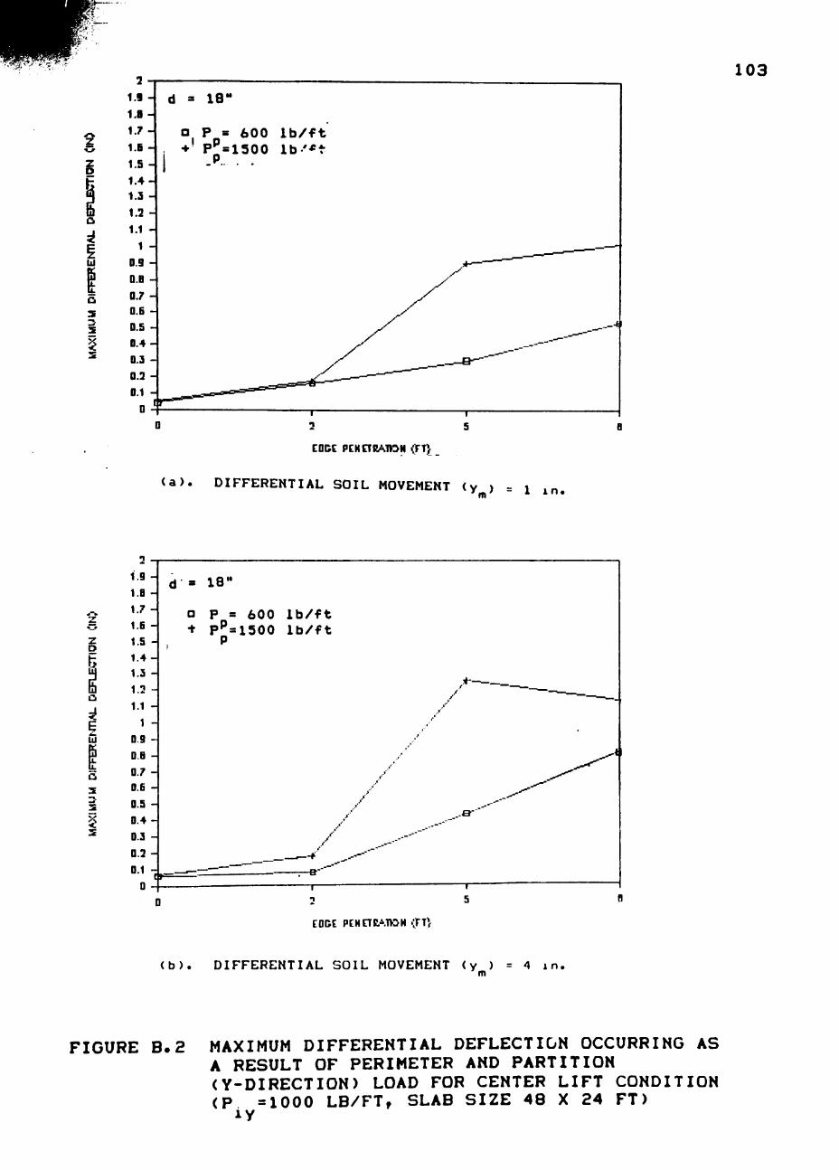
u
a
2?
3 •
1.9 -
1.8
1 7 -
1.E •
1.S
1.4
I.a
1.2
1.1
1
0.9
D.B
0.7
0.6
D.S
0.4
0.3
0.3
0.1
D
103 d = 18'
n P = 600 l b / f t + P > 1 5 0 0 lb '* i -
P. . .
_--i
EOCC PEHCTRAHOH irt}
(a>. DIFFERENTIAL SOIL MOVEMENT (y ) = i .„ ' m * i n .
z D
I u3
<^
1.9
1.B
1.7
1.6
1.5
1.4
1.3
1.3
1.1
1
09
D.B
0.7
O.E
0.5
0.4
0.3
0.3
0.1
0
18"
a P = 600 l b / f t •»• p'^slSOO l b / f t
/
EDCE PEHETB.A.TOM vfT}
(b) DIFFERENTIAL SOIL MOVEMENT = 4 in,
FIGURE B.2 MAXIMUM DIFFERENTIAL DEFLECTION OCCURRING AS A RESULT OF PERIMETER AND PARTITION <Y-DIRECTION) LOAD FOR CENTER LIFT CONDITION <P =1000 LB/FTf SLAB SIZE 48 X 24 FT)
iy

104
z z D
1 lii CJ
3? ^ UI
1 Q S
S
^ s
3
1.9
1.B
1.7
1.6
1.5
1.4 1.3
1.2
1.1
1 0.9 D.B
0.7 0.6
D.S 0.4
0.3
0.3
0.1
0
d = 3 0 '
Q P =
+ Pp=1500 l b / f t 600 l b / f t
__—I
EDCE PEHnPA1>:>H (FT|
( c > . DIFFERENTIAL SOIL MOVEMENT ( y ) = 1 m .
2 O
z o
I b a 3> E z ( i j
1 a 5
S
J 2
3
1.9
1.B
1.7
1.6 1.5
1.4 1.3 1.3
1.1
1 D.g OB
0.7 0.6
0.5
0.4
D.3
0.3
0.1
D
d a 3 0 "
p
600 + P:=I5OO
l b / f t l b / f t
. — — t i
_—-O" — - ^ ' •
- - e -
EOCE PEHCTP.''.n:>H ijV,
( d ) . DIFFERENTIAL SOIL MOVEMENT = 4 I n,
FIGURE B.2 CONTINUED

105
^2
>5
EDG E P E.N' ETHATIO N ' FT)
(a). DIFFERENTIAL SOIL MOVEMENT (v ) = 1 i n .
C'.3
: . 23
-^ . . i s —]
o Ui
u a
UJ a: u
2
a d = 18" + d = 30"
EDGE PENETRATION (FT)
( b ) DIFFERENTIAL SOIL MOVEMENT (y ) = 4 in, m
FIGURE B.3 MAXIMUM DIFFERENTIAL DEFLECTION OCCURRING AS A RESULT OF PERIMETER AND PARTITION LOAD (P =600 LB/FTf f^ =1000 LB/FT), FOR CENTER LIPT CONDITION (SLAB SIZE 48 x 24 FT)

106
cn
- - - -ZiAj-
*> ( « •
00
H E
01
1
G
. c •* ^ II
E >-
. «J «••
t tVJ
H
3
1
o
. «> «•-
fVJ •H
n
cn
v «•-\ a — o o -a H
a OL
«> <*-\ x> - o o o II
- OL.
1
O
1 in
o
00
CO IT
CNI
o M 00 fsl (C M
C>l
<N 04
O
OO
<£)
CM
O
OO
- <o
- - « * -
- (N
O
O
O
u J
CO
<
O
> >-t
< .J UI X
Q Z J <
K
Q
O U
H
O Z
w u • J
X CQ O
< u. in u
u < u,
H cn UJ m m
< • J
z
z o <: • J
UJ cc
u, o z o y-t
H U U W
0.
I 03
UJ
a o
Lu UJ Q
(S3HDMI) H O I l D 3 n J 3 a 3AI1V-I3d

APPENDIX C
PLOTS OF MAXIMUM SHEAR FORCES
107

X
108
3-|d
e -
B -
4. -
C-T
= 18"
• 48 ft slab + 72 ft slab « 9b ft slab
-r-2
-T— A.
EDGE PEN ETHATIO N (FT)
(a). DIFFERENTIAL SOIL MOVEMENT (y ) = i m.
-1 8
10
cn a
2i
-|
E -
5
4. H
:5
2 -4
+
(b).
18"
D 48 ft slab +.72 ft slab « 96 ft slab
-r-2
-r-
EDGE PENETRATION (FT)
DIFFERENTIAL SOIL MOVEMENT (y ) m
4 in.
FIGURE C.1 MAXIMUM SHEAR FORCES OCCURRING AS A RESULT OF PERIMETER .-ND PARTITION (Y-DIRECTION) LOAD FOR CENTER LIFT CONDITION (P =600 LB/FT, P =1000 LB/FT) ^

Q.
Q:
6
a
or
10
9
109
_ d = 30"
B -J
3 -
T _
1 -
• 48 ft slab + 72 ft slab o 96 ft slab
c -r o 1-
2 ^ ^
-r-6
EDGE PENETTRATION (FT )
(c). DIFFERENTIAL SOIL MOVEMENT (y ) = 1 m .
10
g
D 48 ft slab + 72 ft slab 0 96 ft slab
^ -1
3 H
EDGE PENETTIATION (FT )
(d). DIFFERENTIAL SOIL MOVEMENT (y ) = 4 in. m
FIGURE C l CONTINUED

'T: Q.
UJ
o P = 600 l b / f t + P^=1500 l b / f t
R -1
5
110
c• r;c• O C K I L I U> -, . . w . . ... . y
<a). DIFFERENTIAL SOIL MOVEMENT (y ) = 1 in. in
a.
UJ
Ol
c-nr;r DC-MI- IU)ATI,^M /c-T . - w w w . w . , W . . N ^ . . W , , i^, . ,
<b). DIFFERENTIAL SOIL MOVEMENT (v ) = 4 ,„
FIGURE C . 2 MAXIMUM SHEAR FORCES OCCURRING AS A RESULT OF PERIMETER AND PARTITION (Y-DIRECTION) LOAD FOR CENTER LIFT CONDITION (P = 1 0 0 0 LB/FT, SLAB SIZE 4 8 X 24 FT) ^^

a."
10
g
5 -
A. -
d '= 3 0 "
a P = 6 0 0 * l b / f t + P = 1 5 0 0 l b / f t
P
KJ -y-
O T-2 A.
1^
B
EDGE PENETRATION (FT )
111
<c). DIFFERENTIAL SOIL MOVEMENT (y ) m
= 1 i n .
CT u .
UI
d = 3 0 "
c P = 6 0 0 l b / f t + P ^ = 1 5 0 0 l b / f t
P
6 -
S -
A -
2> -
1 - f
O - T " 2
- I — A .
-r-S
cr^.'^F" oc*^-'P~ro ^ y - ^ M ^ PT^
( d ) . DIFFERENTIAL SOIL MOVEMENT (y ) = 4 i n .
a
FIGURE C . 2 CONTINUED

a
UJ X
g -
a -
~ —
6 -
5 -
"^ -r-o
a d = 18" •^• d = 3 0 "
2
EDGE PENETP.ATION (FT)
(a). DIFFERENTIAL SOIL MOVEMENT (y„) = 1 i", m
- I a
112
i o
\
a: <i UJ - 1 . cn
3 -
3 -
B -
6 -
4.-
I I I
^ I I
. J
D d + d
18" 30"
. < ^
-t
- T '-' - r -r
2 A -r-B
' • ' ^ PENETRATION ( . ^ )
- I
a
b). DIFFERENTIAL SOIL MOVEMENT (y^) 4 in.
FIGURE C.3 MAXIMUM SHEAR FORCES OCCURRING AS A RESULT OF PERIMETER AND PARTITION LOAD (P =600 LB/FT, p =1000 LB/FT) FOR CENTER LIFTPCONDITION ( felAB SIZE 48 X 24 FT)

APPENDIX D
PLOTS OF MAXIMUM BENDING MOMENTS
113

1 1 4
CD
. c '-t
t-t
II E
>-
•P «•-
CVJ
II E
01
•P <•-\ n ^^
o II
a CL
+J «•-\ J3 —
o o o r-t 11
0.
Q -< O
z o
J < Q Z UJ •-I U Q < D J H 0. >-« o cn Z H<
o
u X o z o
<
z UJ 2: o z: u. o z o
<
H
<
Q < O
ct:
UJ
UJ
z cx UJ UJ Z CL
cn UJ X <
O
z
Q : UJ «< > > cn z
< a:
UJ 2 tn oc cn
<
u • - »
Q. >•
Q
UJ X
o
Q Z <
X < I
X
o z o <
( I J / S c i l H - l J ) l.WJWOW

c ^///////•yy/////
CD
<•-
CXI
II
OJ
•P
N
O
II
-P
jQ
O O O «—( II
Q.
Hi I-
+1
C\J
II
: i !
r]
ri
CVI II
2
1^
D
Z]
- - D '
. ^ ' - — a ~ " f — +-•
D - — - _ _ V:
• ^ - Q .
- - " t 3
•
Z]
•
. -•-•
I I
n—I—I i r M"! l O - + 1^ ' C l
i I I I I I I I I I . I
•-I iD r- ' f lO -+ f* c I — c r- c I f - i
Cl o izi o i: I I \~\
< z l-H
Q D
Q UJ U <
a. o tn z >-i
o <
UJ o Z J
o z o
<
z UJ
o
o z o
z o
Q <
o • 1 DC H UJ X H < UJ a. "z.
>-t
z tr U UJ Z CL
en u X
H D O
z
H U 3 < cn •-< CK cn PC UJ «-• < > X > cn <
Z I J < > < a: u H o >-t z 0, Q O >- Z J H < <
C\J .
Q
X
1 1 5
I I I
( i J / s d i H - i J ) iHz;^':^;^

CT
O
WJ
s
^
U.
<
2 2
20 -I d = 18"
1S -I Q P = 6 0 0 l b / f t + P ^ = 1 5 0 0 l b / f t
1 6 - 1
116
' -r 1 ^
5 -1 a
EDGE PENETRATION (FT)
(a). DIFFERENTIAL SOIL MOVEMENT (y ) = 1 i"' tn
EDGE PE.NETRATIO.N (FT)
(b). DIFFERENTIAL SOIL MOVEMENT (y ) = 4 in, m
FIGURE D.3 MAXIMUM NEGATIVE MOMENT OCCURRING AS A RESULT OF PERIMETER AND PARTITION (Y-DIRECTION) LOAD FOR CENTER LIFT CONDITION (P^ =1000 LB/FT SLAB SIZE 48 X 24 FT) iy

^ 20 - d = 30
.u.
I
I • I
117
15-1 a P = 600* l b / f t I + P^=1500 l b / f t
IB -J P
1 J. -
12 -
10 -
e -
6 -
A -
/ /
/
EDGE PENETRATION (FT)
(c). DIFFERENTIAL SOIL MOVEMENT (y ) 1 in.
f 1
!
u.
UJ
LU
g
n P = 600 lb/ft
W W W W . _ , . W .. N.I-k. . W . < y . ./
(d). DIFFERENTIAL BOIL MOVEMENT (y_ ) = 4 in.
FIGURE D.3 CONTINUED

118
rn
in
UJ
UJ
T / ^ _
15 -i
16 -I
d = 1 3 "
• 4 3 f t s l a b + 72 f t s l a b '> 96 f t s l a b
EDGE PENETPsATION (FT)
(a). DIFFERENTIAL SOIL MOVEMENT (y ) = I in. m
J d = 18"
ie -
IS -
14. -
12 -
io -
a -
6 -
4. -
2 -
D 48 ft slab + 72 ft slab o 96 ft slab
^
EDGE PENETRATION (FT)
(b). DIFFERENTIAL SOIL MOVEMENT (y^) = 4 in. tn
4
I
-i a
FIGURE D.4 MAXIMUM NEGATIVE MOMENT OCCURRING AS A RESULT OF PERIMETER AND PARTITION (Y-DIRECTION) LOAD FOR CENTER LIFT CONDITION (P =600 LB/FT, P =1000 LB/FT) ^

119
20 -I d 30"
IB -i
UI
'S
18 -I
o An ft slab + 72 ft slab o 96 ft slab
-one- oc-M c-ro Axi/^M ,'c- ^ - w w w . w. . w . . v -k . .w . • .(, . .y
(c). DIFFERENTIAL SOIL MOVEMENT (y ) = 1 m.
d = 30"
15 -
1 e -
1 J. -
I.I -.»• ^ ' ^ _> w—
<
=
— 1
12 -
IO -
a -
t -
A -
a 48 ft slab + 72 ft slab « 96 ft slab
-/
a EDGE PENETRATION (FT )
( d ) . DIFFERENTIAL SOIL MOVEMENT ( y ) = 4 i n ,
FIGURE D.4 CONTINUED

120
u.
?5
J
„J 1 6 -I
IJ. -1
u -r -O
( a )
a d = 1 8 " •(- d = 3 0 "
, • ! • • "
5
EDGE PENETRATION (FT)
D I F F E R E N T I A L S O I L MOVEMENT ( y ) m
= 1 i n ,
-I a
UJ
o
'<^
X.
15 -i
16 -
1.1 -
12
IO -
a —
6 -
A -
w -r-
a d = 18' + d = 3 0 '
5
EDGE PENETTRATION (FT)
( b ) . D I F F E R E N T I A L S O I L MOVEMENT ( y ^ ) = ^ i " '
I
/ I I
a
FIGURE D . 5 MAXIMUM NEGATIVE MOMENT OCCURRING AS A RESULT OF PERIMETER AND PARTITION LOAD (P =600 LB/FT, P. =1000 LB/FT)t FOR CENTER LIFT C6NDITI0N (i^AB SIZE 48 X 24 FT)
APPENDIX E
EXAMPLE PROBLEMS
121

PROBLEM i:
Designed by Using the PTI Method. The slab was designed,
by using a program written by Abdallah (1987). The input
data and the output of the program is given below.
40'-0"
o 1 CD CO.
1
/ /
yV////yy/yyyyy.^yyyyy
PERIMETER LOAD
13'-0" 6'-6" f - 6'-6" tf 14'-0" -I
Design Data.
1. Perimeter Load
2. Live load
(P >= 840 lb/ft P
= 40 psf
(f ')= 2500 psi c
3. Concrete Compressive Strength
4. Prestressing Steel Ultimate Strength = 270 ksi
5. Strand Nominal Area
6. Strand diameter
= .085 sq.in.
= 0.5 in
7. Edge Moisture Variation Distance (e^) = 3 ft
8. Differential Soil swell
122
(y ) = .189 in. m

123
9. Allowable Soil Bearing Pressure
10. Slab-Subgrade Friction
11. Slab Length
12.
13.
14.
15.
Slab Width
= 2700 psf
= .75
(L)= 40 ft
(W)= 38 ft
Modulus of Elasticity of Concrete (E ) c
(E ) s
Modulus of Elasticity of Soil
Required Residual Compressive Strength
25 X 10
1500 psi
at the Center of Slab
16. Slab Thickness
17. Partition load
= 50 psi
(t) = 4 in.
a) P ly
b) P ly
= 840 lb/ft
= 1260 lb/ft
According to PTI (1980) design manual, if the value of
the tensile stress
f = (2.35 P/t^*^^)-fp (D. 1 )
where
P = partition load in lbs/ft
t = thickness of the slab in inch
f = minimum compressive stress in concrete due to P
prestressing (usually 50 psi)
exceeds the allowable tensile stress,
f = 6,/f~ ta V c
(D. 2)
where
f '= concrete compressive stress c

124
then a thicker slab section should be used under the loaded
area, or a stiffening beam should be placed directly beneath
the concentrated line load.
Check whether stiffening beam is required i
a) Partition load (P.) = 840 lb/ft 1
f = (2.35 X 840/ (4^*^^ ) )-50
= 299 psi
f^ = 6 X (2500) ta
.5
= 300 psi
f < f stiffening beam is not required t ta
b) Partition load (P^) = 1260 lb/ft
f = (2.35 X 1260/(t^*^^) - 50
= 473 psi
^ > ^ a stiffenng beam is required
840 lb/ft partition load can be placed on the slab without a
stiffening beam, but 1260 lb/ft perimeter load cannot be
placed without a stiffening beam.
The problem with partition load of 1260 lb/ft is solved
in the PTI method and the results obtained toghether with
the design data were used in the new developed equations to
calculate moemnts, shear forces and differential deflection.

125
Section Properties
Long Short Direction Direction
Moment of Inertia
Cross Sectional Area
Centroids of Strands
Depth to Neutral Axis
Prestressing Eccentricity
Allowable Concrete Tensile Stress (ksi ) (f =6 X ,/r~' )
t V c Allowable Concrete Compressible Stress (ksi) (f =.45 X f ' ) c c
Tensile Cracking Stress (ksi) (F =.75 X jr~' ) cr V c
85808.5
2784.0
-2.0
-5.44
3.45
0.30
1. 125
0.375
102006.3
3120.0
-2.0
-5.85
3.84
0.30
1. 125
0.375
Calculation Summary
1. Moment (ft-kips/ft)
Short Direction
Tensi le
Compressive
Cracking
Long Direction
Tensi le
Compressive
2. Differential Deflection (inches)
Pes iqn Allowab1e
2. 58 <
2.58 <
2.58 <
2. 53
12. 13
12. 16
14. 58
11. 35
2.54 < 10.42
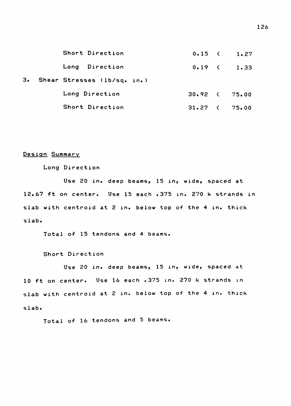
126
S h o r t D i r e c t i o n 0.15 < 1.27
Long Direction 0.19 < 1.33
3. Shear Stresses (Ib/sq. in.)
Long Direction 30.92 < 75.00
Short Direction 31.27 < 75.00
Design Summary
Long Direction
Use 20 in. deep beams, 15 in, wide, spaced at
12.67 ft on center. Use 15 each .375 in. 270 k strands in
slab with centroid at 2 in. below top of the 4 in. thick
slab.
Total of 15 tendons and 4 beams.
Short Direction
Use 20 in. deep beams, 15 in, wide, spaced at
10 ft on center. Use 16 each .375 in. 270 k strands in
slab with centroid at 2 in. below top of the 4 in. thick
slab.
Total of 16 tendons and 5 beams.

127
Designed by Using The New Developed Equations.
Design Data.
1.
2.
3.
4.
12.
13.
14.
15.
Perimeter Load
Live load
(P )= 840 lb/ft P
= 40 psf
(f ')= 2500 psi c ^ Concrete Compressive Strength
Prestressing Steel Ultimate Strength = 270 ksi
5. Strand Nominal Area
6. Strand nominal Diameter
= .085 sq.1n
= 0.5 in
7. Edge Moisture Variation Distance (e ) = 3 ft m
8. Differential Soil swell
9. Allowable Soil Bearing Pressure
10. Slab-Subgrade Friction
11. Slab Length
Slab Width
(y ) = .189 in. •m
= 2700 psf
= .75
(L)= 40 ft
(W)= 38 ft
Modulus of Elasticity of Concrete (E ) c
(E ) s
Modulus of Elasticity of Soil
Required Residual Compressive Strength
25 X 10
1500 psi
at the Center of Slab
16. Slab Thickness
= 50 psi
(t) = 4 in.
Additional design parameters are taken from the
previous problem in order to compare the results, resulting
from the solution by two different methods.
17. Beam depth (d) = 20 in.

128
18. Beam width <W) = 15 ^^^
19. Beam spacing x-direction (S ) = 12.67 ft
20. Beam spacing y-direction (S ) = 10 ft y
21. Partition load (P >= 126O lb/ft
The design data are used to calculate moments, shear
forces and differential deflection with the following
equations.
' ( L ) - ° ' ^ <S ' ) - ^ ^ ^ < d ) - 3 ' ' ' ' ( . ) 1 - 1 0 ^ <P , - 8 9 2 ^p , . 1 0 2 ^p , . 1 0 4 ..X •» P i x l y
M • 0 .00029 . . ^ « X VJ.UUWCT ( D . 3 )
/ , . 0 3 2
< L ) - 2 ^ 5 , ^ , . 3 5 3 ^^ , 1 . 1 0 8 ^p , . 9 7 0 ^p , . 0 8 6 ^p , . 0 7 3
M^ - 1 . 6 0 9 ^ . ! ! p _ * * ' y y . ( D . 4 )
<y„>*°^^ <s )3-^6< m ^
V - 3 .5£ ( D . S ) X . , . 0 5 4
( m
<t.,-'^^ . . . • " ' < . „ . • " = < p „ ' - ' ' ' < ^ . ' • " ' < ' . v ' - ° " V a 0 . 4 0 7 <D. 6 )
<L>-=" <e >^-^'^ < r „ . - ° " < P p ' - ' " ' ^ , > - ' " ' ^ v ' - ^ ° '
A . = 0. 077 •X - «• — ' 1 . 3 8 9 1 . 1 6 9 (D.7) (S ) <= '
X
. 3 4 5 , . , 1 . 3 1 6 , , , . 0 6 1 ^p , . B 2 & ^p . 1 0 5 c p _ ) - ' 0 6 <S >- = -^2 ( L ) - ^ ' ^ ^ ( e , ) ^ * - " <y„ ) ^^p^ ^ ^ x ' ^ ^ l y ' ^"y
re
^ n 0 .00029 — ; ^ ^ g y ( d )
(D. 8)

w^.^ • # ' ^
»» i .-. . ^fT
129
Partition Load (P ) iy
= 1260 lb/ft
M^ (ft-kips/ft)
M (ft-kips/ft)
V^ (kips/ft)
V (kips/ft)
Aa, (inch)
A (inch)
Design
3«69
8.03 <
66.10 i
81.26 :
0.167 <
0.145 <
Allowable
C 12.46
C 13.49
: 75.00
• 75.00
: 1.33
1.27
PROBLEM 2:
PTI DESIGN METHOD
— 42
OJ
" ^ ^' V^-^ /••->////. / - Z Z Z Z Z z ^ .
/ / /
/ PARTITION LOAD
/
"///yy////// PERIMETER LOAD
//y /////y//^/ '•"' I
tf •16' If 13' =tf 13'
(Vi v-l
4) X
(U
Design Data?
1. Perimeter load (P^)= 1040 lb/ft P
2. Live Load = 40 psf
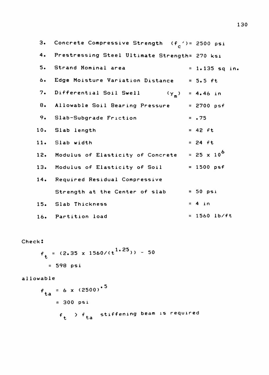
130
3. Concrete Compressive Strength (f ')= 2500 psi
4. Prestressing Steel Ultimate Strength= 270 ksi
5. Strand Nominal area
6. Edge Moisture Variation Distance
m 7. Differential Soil Swell
8. Allowable Soil Bearing Pressure
9. Slab-Subgrade Friction
10. Slab length
11. Slab width
12. Modulus of Elasticity of Concrete
13. Modulus of Elasticity of Soil
14. Required Residual Compressive
Strength at the Center of slab
15. Slab Thickness
16. Partition load
= 1. 135 sq in.
= 5.5 ft
= 4.46 in
= 2700 psf
= .75
= 42 ft
= 24 ft
= 25 x 10^
= 1500 psf
= 50 psi
= 4 in
= 1560 lb/ft
Check:
f = (2.35 X 1560/(t^*^^)) - 50
= 598 psi
allowable
f = 6 X (2500) ta
= 300 psi
.5
f > f stiffening beam is required

Section Properties
131
Moment of Inertia
Cross Sectional Area
Centroids of Strands
Depth to Neutral Axis
Prestressing Eccentricity
Allowable Concrete Tensile Stress (ksi)
Long Short Direction Direction
131447.90
2124.00
-2.00
-8.008
6.008
0.30
Allowable Concrete Compressible Stress (ksi) (f = .45 X f ')
c c
Tensile Cracking Stress (ksi)
cr
1. 125
0.375
190739.91
3336.00
-2.00
-7. 14
5. 143
0.30
1. 125
0.375 (F = .75 X ^f^')
Calculation Summary
1. Moment (ft-kips/ft)
Short Direction
Tensile
Compressive
Cracking
Long Direction
Tensi le
Compressive
Design Allowab 1 e
1 3 . 8 4 < 2 4 . 1 2
1 3 . 8 3 < 2 3 . 8 9
1 3 . 8 3 < 2 8 . 07
1 3 . 0 7 < 2 3 . 4 7
1 3 . 0 7 < 2 9 . 7 5
2. Differential Deflection

132
Short Direction .53 < .80
Long Direction .63 < 1.40
3. Shear Stress (Ib/sq.in)
Short Direction 46.50 < 75.00
Long Direction 54.21 < 75.00
Design Summary
Long Direction
Use 26 inch deep beams, 15 inch wide, spaced at 12
ft on center. Use 1 each .5 in 270 k strands in slab with
centroid at 2 inch below top of the 4 inch thick slab.
Total of 1 tendons and 3 beams.
Short Direction
Use 26 inch deep beams, 15 inch wide, spaced at 14
ft on center. Use 2 each 0.5 inch 270 k strands in slab
with centroid at 2 inch below top of the 4 inch thick slab.
Total of 2 Tendons and 4 beams.
Designed by Using the new Developed Equations.
Design Data
1.
2.
3.
4.
Perimeter load ^^p^"
Live Load
Concrete Compressive Strength (f^')=
Prestressing Steel Ultimate Strength=
1040 lb/ft
40 psf
2500 psi
270 ksi

133
5. Strand Nominal area
6. Edge Moisture Variation Distance
(y ) • m
7. Differential Soil Swell
8. Allowable Soil Bearing Pressure
9. Slab-Subgrade Friction
10. Slab Length
11. Slab Width
12. Modulus of Elasticity of Concrete
13. Modulus of Elasticity of Soil
14. Required Residual Compressive
Strength at the Center of slab
15. Slab Thickness
16. Partition load
17. Beam Depth
18. Beam width
= 1.135 sq in
= 5.5 ft
= 4.46 in
= 2700 psf
= .75
= 42 ft
= 24 ft
= 25 X 10^
= 1500 psf
= 50 psi
= 4 1 n
= 1560 lb/ft
= 26 in.
= 15 in.
(S ) = 1 2 ft X
(S ) = 1 4 ft y
19. Beam Spacing x-direction
20. Beam Spacing y-direction
Substituting the above data in the Equations D-3 to D-8 we
get the following values
Results:
Partition Load (P^ ) = 1560 lb/ft
M (ft-kips/ft) X
M (ft-kips/ft) y
Design
8.72
6. 04
Allowab1e
24. 12
23. 89

134
V (kips/ft) X
V (kips/ft) y
•^x ( inch )
-^y ( inch )
68. 10
35.26
0. 187
0.445
75.00
75.00
.80
1.40
COMMENTS
Prob lem 1
Calculating the moments, shear forces and differential
deflection values with the new developed equations in this
study for 1260 lb/ft partition load, it is observed that
only the value of the shear stress in the y-direction (page
129) exceeds the allowable value and all the other
calculated values are less then the allowable. To reduce
the shear stress the beam width of 15 in. in the problem
should be increased.
Problem 2.
In the second problem the values (page 133) calculated
from the eqautions are less then the allowable values. So
these values can be used in the design of the slab with
perimeter load.

PERMISSION TO COPY
In presenting this thesis in partial fulfillment of the
requirements for a master's degree at Texas Tech University. I agree
that the Library and my major department shall make it freely avail
able for research purposes. Permission to copy this thesis for
scholarly purposes may be granted by the Director of the Library or
my major professor. It is understood that any copying or publication
of this thesis for financial gain shall not be allowed without my
further written permission and that any user inay be liable for copy
right Infringement.
Disagree (Permission not granted) Agree (Permission granted)
Student's signature Student's signature
Date Date ng/ai/g^


