
Copyright Warning & Restrictions
The copyright law of the United States (Title 17, United States Code) governs the making of photocopies or other
reproductions of copyrighted material.
Under certain conditions specified in the law, libraries and archives are authorized to furnish a photocopy or other
reproduction. One of these specified conditions is that the photocopy or reproduction is not to be “used for any
purpose other than private study, scholarship, or research.” If a, user makes a request for, or later uses, a photocopy or reproduction for purposes in excess of “fair use” that user
may be liable for copyright infringement,
This institution reserves the right to refuse to accept a copying order if, in its judgment, fulfillment of the order
would involve violation of copyright law.
Please Note: The author retains the copyright while the New Jersey Institute of Technology reserves the right to
distribute this thesis or dissertation
Printing note: If you do not wish to print this page, then select “Pages from: first page # to: last page #” on the print dialog screen

The Van Houten library has removed some ofthe personal information and all signatures fromthe approval page and biographical sketches oftheses and dissertations in order to protect theidentity of NJIT graduates and faculty.

ABSTRACT
TARGET LOCALIZATION IN MIMO RADAR SYSTEMS
byHana Godrich
MIMO (Multiple-Input Multiple-Output) radar systems employ multiple antennas to
transmit multiple waveforms and engage in joint processing of the received echoes from
the target. MIMO radar has been receiving increasing attention in recent years from
researchers, practitioners, and funding agencies. Elements of MIMO radar have the ability
to transmit diverse waveforms ranging from independent to fully correlated. MIMO radar
offers a new paradigm for signal processing research. In this dissertation, target localization
accuracy performance, attainable by the use of MIMO radar systems, configured with
multiple transmit and receive sensors, widely distributed over an area, are studied. The
Cramer-Rao lower bound (CRLB) for target localization accuracy is developed for both
coherent and noncoherent processing. The CRLB is shown to be inversely proportional
to the signal effective bandwidth in the noncoherent case, but is approximately inversely
proportional to the carrier frequency in the coherent case. It is shown that optimization over
the sensors' positions lowers the CRLB by a factor equal to the product of the number of
transmitting and receiving sensors. The best linear unbiased estimator (BLUE) is derived
for the MIMO target localization problem. The BLUE's utility is in providing a closed-form
localization estimate that facilitates the analysis of the relations between sensors locations,
target location, and localization accuracy. Geometric dilution of precision (GDOP)
contours are used to map the relative performance accuracy for a given layout of radars
over a given geographic area. Coherent processing advantage for target localization relies
on time and phase synchronization between transmitting and receiving radars. An analysis
of the sensitivity of the localization performance with respect to the variance of phase
synchronization error is provided by deriving the hybrid CRLB. The single target case
is extended to the evaluation of multiple target localization performance. Thus far, the

analysis assumes a stationary target. Study of moving target tracking capabilities is
offered through the use of the Bayesian CRLB for the estimation of both target location
and velocity. Centralized and decentralized tracking algorithms, inherit to distributed
MIMO radar architecture, are proposed and evaluated. It is shown that communication
requirements and processing load may be reduced at a relatively low performance cost.

TARGET LOCALIZATION IN MIMO RADAR SYSTEMS
byHana Godrich
A DissertationSubmitted to the Faculty of
New Jersey Institute of Technologyin Partial Fulfillment of the Requirements for the Degree of
Doctor of Philosophy in Electrical Engineering
Department of Electrical and Computer Engineering
January 2010

Copyright © 2010 by Hana Godrich
ALL RIGHTS RESERVED

APPROVAL PAGE
TARGET LOCALIZATION IN MIMO RADAR SYSTEMS
Hana Godrich
Dr. Alexander M. Haimovich, Dissertation Advisor DateProfessor, Department of Electrical and Computer Engineering, NJIT
Dr. Yeheskel Bar-Ness, Committee Member DateDistinguished Professor, Department of Electrical and Computer Engineering, NJIT
Dr. Ali Abdi , Committee Member DateAssociate Professor, Department of Electrical and Computer Engineering, NJIT
Dr. Osvaldo Simeone, Committee Member DateAssistant Professor, Department of Electrical and Computer Engineering, NJIT
Dr. Rick S. Blum , Committee Member DateProfessor, Department of Electrical and Computer Engineering, Lehigh University
BIOGRAPHICAL SKETCH
Author: Hana Godrich
Degree: Doctor of Philosophy
Date: January 2010
Undergraduate and Graduate Education:
• Doctor of Philosophy in Electrical Engineering,New Jersey Institute of Technology, Newark, NJ, 2010
• Master of Science in Electrical Engineering,Ben-Gurion University, Beer-Sheva, Israel, 1993
• Bachelor of Science in Electrical Engineering,Technion Israel Institute of Technology, Haifa, Israel, 1987
Major: Electrical Engineering
Presentations and Publications:
H. Godrich, A. M Haimovich and R. S. Blum, "Concepts and applications of a MIMOradar system with widely separated antennas," book chapter in MIMO Radars, JohnWiley, January 2009.
H. Godrich, A. M. Haimovich, and R. S. Blum, "Target localisation techniques and tools formultiple-input multiple-output radar," in IET Radar; Sonar and Navigation, Vol.3,August 2009, pp. 314-327.
H. Godrich, A. M. Haimovich, and R. S. Blum, "Target localization accuracy gain in MIMOradar based system," to appear in IEEE Trans. on Information Theory.
H. Godrich, A. M. Haimovich, and R. S. Blum, "Target tracking in MIMO radar systems:techniques and performance analysis," submitted to IEEE Radar Conf. May, 2010.
H. Godrich, A. M. Haimovich, and H. V. Poor, "An analysis of phase synchronizationmismatch sensitivity for coherent MIMO radar systems," to appear in Proc. ofthe Third International Workshop on Computational Advances in Multi-SensorAdaptive Processing (CAMSAP), December 2009.
iv

H. Godrich, A. M. Haimovich, and R. S. Blum, "A MIMO radar system approach to targettracking," in Proc. of 43th Asilomar Conf. Signals, Syst. Comput., November 2009.
H. Godrich, A. M. Haimovich, and R. S. Blum, "A comparative study of target localizationin MIMO radar systems," in IEEE Intl. Waveform Diversity and Design Conf.,February 2009,pp. 124-128.
H. Godrich, A. M. Haimovich, and R. S. Blum, "Target localization accuracy and multipletarget localization: tradeoffs in MIMO radars," in Proc. of 42th Asilomar Conf.Signals, Syst. Comput., October 2008, pp. 614-618.
H. Godrich, A. M Haimovich, and R. S. Blum, "Target localization techniques and toolsfor MIMO radar," in IEEE Radar Conf. , May, 2008, pp. 1-6.
H. Godrich, A. M. Haimovich, and R. S. Blum, "Cramer Rao bound on target localizationestimation in MIMO radar systems," in Proc. of 42nd Annual Conference oninformation Sciences and Systems (CISS) 2008, March 2008, pp. 134-139.
Q. He, R. S. Blum, H. Godrich, and A. M. Haimovich, "Cramer-Rao bound for targetvelocity estimation in MIMO radar with widely separated antennas," in Proc. of42nd Annual Conference on information Sciences and Systems (CISS) 2008, March2008, pp. 123-127.
Q. He, R. S. Blum, H. Godrich, and A. M. Haimovich, " Target velocity estimation andantenna placement for MIMO radar with widely separated antennas," to appear inIEEE Journal of Selected Topics in Signal Processing.

To Kfir, Ran, Dana, and Noawith Love
vi

ACKNOWLEDGMENT
"Destiny is not a matter of chance, it is a matter of choice;
it is not a thing to be waited for it is a thing to be achieved."
[Winston Churchill]
To make things happen, one not only needs to take on his own destiny, but also to be
blessed with the support of wonderful people along the way. I would like to express my
deepest appreciation to my adviser, committee chair, and mentor, Dr. Alexander Haimovich
who has opened the doors for me and made all of this possible. Without his confidence,
support and inspiration this dissertation would not have been possible. It has been a joy and
challenge to work with him in developing the ideas in this thesis. Special thanks to Dr. Rick
Blum for partnering with Dr. Alexander Haimovich and me in this research collaboration
and for serving on my committee. I would like to thank Dr. Yeheskel Bar-Ness, Dr. All
Abdi, and Dr. Osvaldo Simeone for serving on my dissertation committee. Extended thanks
to Dr. Nikolaus Lehmann for sharing his thoughts, his helpful advice and all the more, for
his friendships.
"It is the supreme art of the teacher to awaken joy in creative expression and
knowledge." [Albert Einstein]
To the professors at NJIT that have taught me along the way, my sincere gratitude:
Dr. Yeheskel Bar-Ness for sharing his extensive knowledge in wireless communication,
Dr. Alexander Haimovich for breaking information theory to an understandable level, Dr.
Osvaldo Simeone, who makes convex optimization looks so clear and simple - I have put
the thing I have learned from him to very good use in this thesis, Dr. Richard Haddad
for his inspirational teaching and personality, and Dr. Ali Akansu and Dr. Hongya Ge for
providing me with extensive signal processing tools.
vii

The amazing woman that takes care of all of us in the CWCSPR Center, Ms. Marlene
Toeroek, deserves special acknowledgment. We would all be lost without her — she takes
care of things before we even know it.
Special thanks are extended to Dr. Ronald Kane, Ms. Clarisa Gonzalez, the staff
at the graduate studies office of NJIT, Mr. Jeffrey Grundy, the staff at the international
student and faculty, Ms. Marlene Massie, and Ms. Jacinth. Williams that provided advice
and support in all administrative matters during my doctoral studies.
A penultimate thank you goes to my wonderful parents and extended family for
always being there for me.
My final, and most heartfelt, acknowledgment must go to my children, Ran, Dana and
Noa for being remarkably patient and understanding to the late night courses and endless
working hours, and my love and best friend, Kfir, for being the rock in my life and taking
care of me every step of the way.
Viii
TABLE OF CONTENTS
Chapter
1 INTRODUCTION
1.1 MIMO Radar Background
1.2 Dissertation Main Contributions
Page
1
1
4
1.2.1 Lower Bound on Target Localization 4
1.2.2 Spatial Advantage Optimization and Analysis 5
1.2.3 CRLB for Multiple Target Localization 6
1.2.4 Sensitivity Analysis of Coherent Processing to PhaseSynchronization Errors 7
1.2.5 Bayesian Cramer-Rao Bound (BCRB) for Target Tracking 7
1.3 Dissertation Outline 8
2 TARGET LOCALIZATION IN MIMO RADAR 10
2.1 Introduction 10
2.2 System Model 10
2.3 Localization CRLB 15
2.3.1 Noncoherent Processing CRLB 17
2.3.2 Coherent Processing CRLB 22
2.3.3 Discussion 26
2.4 Effect of Sensor Locations 29
2.4.1 Optimization Problem 30
2.4.2 Discussion 38
3 METHODS FOR TARGET LOCALIZATION 40
3.1 BLUE for Noncoherent and Coherent Target Localization 40
3.1.1 BLUE for Noncoherent Processing 42
3.1.2 BLUE for Coherent Processing 44
3.1.3 Discussion 47
ix
TABLE OF CONTENTS(Continued)
Chapter
3.2 Generalization for MIMO and SIMO Coherent Localization
Page
48
3.2.1 MIMO Radar 48
3.2.2 SIMO Radar 50
3.2.3 Discussion 52
3.3 GDOP 52
3.3.1 GDOP for MIMO 53
3.3.2 GDOP for SIMO 58
3.4 Conclusions 62
4 MULTIPLE TARGETS LOCALIZATION 64
4.1 System Model 64
4.2 The CRLB on Targets Location Estimation 67
4.3 Discussion 70
4.4 Numerical Analysis 72
4.5 Conclusions 76
5 SENSITIVITY ANALYSIS TO PHASE SYNCHRONIZATION MISMATCH 78
5.1 Background 79
5.2 HCRB with Phase Mismatch 80
5.3 Numerical Analysis 86
5.4 Conclusions 87
6 TARGET TRACKING IN MIMO RADAR SYSTEMS 89
6.1 System Model 90
6.2 The Bayesian Cramer-Rao Bound (BCRB) 94
6.3 Numerical Analysis 97
6.4 Tracking Algorithms 101
6.4.1 Centralized Tracking 102
TABLE OF CONTENTS(Continued)
Chapter Page
6.4.2 Decentralized Tracking 105
6.5 Conclusions 108
7 CONCLUSION AND FUTURE WORK 109
APPENDIX A CRLB FOR NON-COHERENT PROCESSING 113
APPENDIX B CRLB FOR COHERENT PROCESSING 115
APPENDIX C DERIVATION OF ERROR COVARIANCE MATRIX FOR TIMEOBSERVATIONS 118
C.1 Noncoherent Processing 118
C.2 Coherent Processing 120
APPENDIX D DERIVATION OF FIM MATRIX FOR PHASE SENSATIVITYANALYSIS 122
APPENDIX E DERIVATION OF FIM MATRIX FOR THE BCRB 125
REFERENCES 127
xi
LIST OF TABLES
Table Page
6.1 Centralized Tracking 104
6.2 Decentralized Tracking Algorithm 107
xii
LIST OF FIGURES
Figure Page
2.1 System Layout. 14
2.2 Transmiter - receiver path. 19
3.1 Noncoherent GDOP contours with M=N=4. 55
3.2 Coherent GDOP contours with M=N=4. 56
3.3 Coherent HxDOP contours with M=N=4. 57
3.4 Coherent HyDOP contours with M=N=4. 57
3.5 Noncoherent GDOP contours with M=N=4 - asymmetrical placement ofradars. 58
3.6 Coherent GDOP contours with M=N=4 - asymmetrical placement of radars. 59
3.7 GDOP contour maps for coherent MIMO radar with M = 3 transmitters andN = 5 receivers - case I. 60
3.8 GDOP contour maps for coherent SIMO radar with M 1 transmitter andN = 15 receivers - case I. 60
3.9 GDOP contour maps for coherent MIMO radar with M = 3 transmitters andN = 5 receivers - caseII . 61
3.10 GDOP contour maps for coherent SIMO radar with M = 1 transmitter andN = 15 receivers - case II. 62
4.1 Multiplr targets signal model. 65
4.2 Spatial advantage values for the case of M=3 transmitter and N=3, 4, and 5receivers, symmetrically positioned around the axis origin. 74
4.3 Spatial advantage values in x and y for the case of M=3 transmitter and N=3,4, and 5 receivers, symmetrically positioned around the axis origin. . . . . 74
4.4 System layout for cases 1 to 4. 75
4.5 Spatial advantage values for cases 1 to 4. 76
5.1 HCRB for M=11 and N=9. The blue line represent the CRB value with nophase errors. 87
6.1 Tracking system layout. 92
6.2 Scenario I: 6x4 MIMO radar system with different angular spreads. 97
LIST OF FIGURES(Continued)
Figure Page
6.3 BCRB on target location tracking for scenario I. 98
6.4 BCRB on target velocity tracking for scenario I. 98
6.5 Scenario II: Various symmetrical MIMO radar configurations: (1) 3x4. (2)6x4. (3) 12x4 (4) 18x4. 99
6.6 BCRB on target location tracking for scenario II 100
6.7 BCRB on target location tracking for scenario I. 100
6.8 BCRB on target location tracking for scenario I, with receivers one and twoexperiencing different levels of path loss. 101
6.9 BCRB on target location tracking for centralized and decentralized trackingand the EKF and hybrid KF performance. 106
6.10 BCRB on target location tracking for centralized and decentralized trackingwith different decentralized algorithms 106
xiv

CHAPTER 1
INTRODUCTION
1.1 MIMO Radar Background
Research in MIMO radar has been growing as evidenced by an increasing body of literature
[1-25]. Generally speaking, MIMO radar systems employ multiple antennas to transmit
multiple waveforms and engage in joint processing of the received echoes from the target.
Two main MIMO radar architectures have evolved: with collocated antennas and with
distributed antennas. MIMO radar with collocated antennas makes use of waveform
diversity [4,5,13,15,19], while MIMO radar with distributed antenna takes advantage of the
spatial diversity supported by the system configuration [1, 2, 6,14]. MIMO radar systems
have been shown to offer considerable advantages over traditional radars in various aspects
of radar operation, such as the detection of slow moving targets by exploiting Doppler
estimates from multiple directions [17], the ability to identify and separate multiple
targets [11, 12], and in the estimation of target parameters, such as direction-of-arrival
(DOA) [9, 11], and range-based target localization [18]. In particular, [18] studies target
localization with MIMO radar systems utilizing sensors distributed over a wide area.
Conventional localization techniques include time-of-arrival (TOA), time-difference-
of-arrival (TDOA), and direction-of-arrival (DOA) based schemes. MIMO radar system
with collocated antennas can perform DOA estimation of targets in the far-field, in which
case, the received signal has a planar wavefront. Extensive research has focused on
waveform optimization. In [8, 15, 19] the signal vector transmitted by a MIMO radar
system is designed to minimize the cross-correlation of the signals bounced from various
targets to improve the parameter estimation accuracy in multiple target schemes. Some
of the waveform optimization techniques suggested in [16] are based on the Cramer-Rao
lower bound (CRLB) matrix. The CRLB is known to provide a tight bound on parameter
1

2
estimation for high signal-to-noise ratio (SNR) [26-28]. Several design criteria are
considered, such as minimizing the trace, determinant, and the largest eigenvalue of the
CRLB matrix, concluding that minimizing the trace of the CRLB gives a good overall
performance in terms of lowering the CRLB. In [10], a CRLB evaluation of the achievable
angular accuracy is derived for linear arrays with orthogonal signals. The use of orthogonal
signals is shown to provide better accuracy than correlated signals. For low-SNR scenarios,
the Barankin bound is derived in [11], demonstrating that the use of orthogonal signals
results in a lower SNR threshold for transitioning into the region of higher estimation error.
In all, the CRLB is limited to the analysis of the angular accuracy and therefore the results
cannot be transformed into an equivalent error in a Cartesian coordinate system.
MIMO radar systems with widely spread antennas take advantage of the geographical
spread of the deployed sensors. The multiple propagation paths, created by the transmitted
waveforms and echoes from scatterers, support target localization through either direct
or indirect multilateration. With direct multilateration, the observations collected by
the sensors are jointly processed to produce the localization estimate. With indirect
multilateration, the TOAs are estimated first, and the localization is subsequently estimated
from the TOAs. The observations and processing of the time delays can be classified
as either non-coherent or coherent. Thus, a transmitted signal may have in-phase and
quadrature components, yet the localization processing is non-coherent if it utilizes
only information in the signal envelope. In the sequel, the performance of localization
utilizing both coherent and non-coherent processing is evaluated. The distinction between
the two modes, in terms of system requirements, relies on the need for mere time
synchronization between the transmitting and receiving radars in the non-coherent case,
versus the need for both time and phase synchronization in the coherent case. Note that our
coherent/non-coherent terminology is limited to the processing for localization.
MIMO radar systems belongs to the class of active localization systems, where
the signal usually travels a round trip, i.e., the signal transmitted by one sensor in a

3
radar system is reflected by the target, and measured by the same or a different sensor.
Traditional single-antenna radar systems, performing active range-based measurements, are
well known in literature [29-33]. The target range is computed from the time it takes for the
transmitted signal to get to the target, plus the travelling time of the reflected signal back to
the sensor. The range estimation accuracy is directly proportional to the mean squared error
(MSE) of the time delay estimation and is shown to be inversely proportional to the signal
effective bandwidth [29]. A first study of the localization accuracy capability of widely
spread MIMO radar systems is provided in [18], where the Fisher information matrix
(FIM) is derived for the case of orthogonal signals with coherent processing and widely
separated antennas. The CRLB is analyzed numerically, pointing out the dependency of the
accuracy on the signal carrier frequency in the coherent case, and its reliance on the relative
locations of the target and sensors. In [18], it is observed that the CRLB is a function of
the number of transmitting and receiving sensors, however an analytical relation is not
developed. The high accuracy capability of coherent processing is illustrated by the use
of the ambiguity function (AF). Active range-based target localization techniques are also
used in multi-static radar systems, proposed in [34]. The TOA of a signal transmitted by
a single transmit radar, reflected by the target and received at multiple receive antennas
is used in the localization process. The CRLB is developed for non-coherent processing.
It is observed that increasing the number of sensors improves localization performance,
yet an exact relation is not specified. In [35] the Bayesian Cramer-Rao bound (BCRB) is
developed for the same scheme as in [34]. Simulation-based results show that accuracy
performance depends on the geometric setting of the system, nonetheless a notion of this
effect is not provided. The multi-static scheme evaluated in [34] and [35] does not deal with
the processing of multiple received signals since only one waveform is transmitted. This
dissertation addresses deficiencies in the literature by obtaining closed-form expressions of
the CRLB for both coherent and non-coherent cases with multiple widely spread transmit
and receive radars.

4
Geolocation techniques have been the subject of extensive research. Geolocation
belongs to the class of passive localization systems, where the signal travels one-way. Since
these passive measurement systems employ multiple sensors [36-40], further evaluation of
existing results for geolocation systems may provide insight for the active case. In wireless
communication, passive measurements are used by multiple base stations for localization of
a radiating mobile phone. The localization accuracy performance is evaluated in [36, 38].
It is shown that the localization accuracy is inversely proportional to the signal effective
bandwidth, as it does in the active localization case. Moreover, the accuracy estimation
is shown to be dependent on the sensors/base stations locations. In navigation systems,
the target makes use of time-synchronized transmission from multiple Global Positioning
Systems (GPS) to establish its location. In [39] and [40], the relation between the
transmitting sensors location and the target localization performance is analyzed. GDOP
plots are used to demonstrate the dependency of the attainable accuracy on the location of
the GPS systems with respect to the target. In an optimal setting of the GPS systems relative
to the target position, the best achievable accuracy is shown to be inversely proportional to
the square root of the number of participating GPS sensors. In this research work, the
GDOP metric is utilized in the evaluation of localization performance of MIMO radar
systems.
1.2 Dissertation Main Contributions
The main contributions of this research work are as follows:
1.2.1 Lower Bound on Target Localization
I. The CRLB of the target localization estimation error is developed for the general
case of MIMO radar with multiple waveforms with non-coherent and coherent
observations. The analytical expressions of the CRLB are derived for the case of
orthogonal waveforms (in [3] and [42, 43]).
5
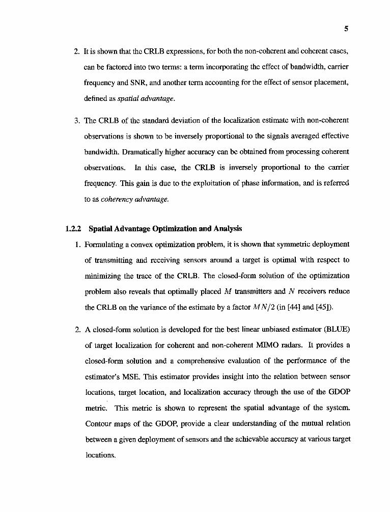
2. It is shown that the CRLB expressions, for both the non-coherent and coherent cases,
can be factored into two terms: a term incorporating the effect of bandwidth, carrier
frequency and SNR, and another term accounting for the effect of sensor placement,
defined as spatial advantage.
3. The CRLB of the standard deviation of the localization estimate with non-coherent
observations is shown to be inversely proportional to the signals averaged effective
bandwidth. Dramatically higher accuracy can be obtained from processing coherent
observations. In this case, the CRLB is inversely proportional to the carrier
frequency. This gain is due to the exploitation of phase information, and is referred
to as coherency advantage.
1.2.2 Spatial Advantage Optimization and Analysis
1. Formulating a convex optimization problem, it is shown that symmetric deployment
of transmitting and receiving sensors around a target is optimal with respect to
minimizing the trace of the CRLB. The closed-form solution of the optimization
problem also reveals that optimally placed M transmitters and N receivers reduce
the CRLB on the variance of the estimate by a factor MN/2 (in [44] and [451).
2. A closed-form solution is developed for the best linear unbiased estimator (BLUE)
of target localization for coherent and non-coherent MIMO radars. It provides a
closed-form solution and a comprehensive evaluation of the performance of the
estimator's MSE. This estimator provides insight into the relation between sensor
locations, target location, and localization accuracy through the use of the GDOP
metric. This metric is shown to represent the spatial advantage of the system.
Contour maps of the GDOP, provide a clear understanding of the mutual relation
between a given deployment of sensors and the achievable accuracy at various target
locations.
6
3. An evaluation of target localization performances for MIMO radar with coherent
processing and single-input multiple-output (SIMO) radar systems, based on the
BLUE, is provided. The best achievable accuracy for both configurations is derived.
MIMO radar systems with coherent processing are shown to benefit from higher
spatial advantage, compared with S1140 systems. The advantage of the MLMO
radar scheme over SLMO is evident when considering the achievable accuracy for
a radar system with M transmitters and N receivers, rather than 1 transmitter and
MN receivers. It is shown that MEMO radar, with a total of M N sensors, has
twice the performance (in terms of localization MSE) of a system with (MN ± 1)
sensors (in [46]).
1.2.3 CRLB for Multiple Target Localization
1. The localization performance study is extended to the case of multiple targets,
with coherent processing. The CRLB for the multiple targets localization problem
is derived and analyzed. The localization is shown to benefit from coherency
advantage. The trade-off between target localization accuracy and the number of
targets that can be localized is shown to be incorporated in the spatial advantage
term.
2. An increase in the number of targets to be localized exposes the system to increased
mutual interferences. This trade-off depends on the geometric footprint of both the
sensors and the targets, and the relative positions of the two. Numerical analysis
of some special cases offers an insight to the mutual relation between a given
deployment of radars and targets and the spatial advantage it presents (in [47]).

7
1.2.4 Sensitivity Analysis of Coherent Processing to Phase Synchronization Errors
1. The hybrid Cramer-Rao bound (CRB) is developed for target localization, to
establish the sensitivity of the estimation mean-square error (MSE) to the level
of phase synchronization mismatch in coherent Multiple-Input Multiple-Output
(MIMO) radar systems with widely distributed antennas. The lower bound on
the MSE is derived for the joint estimation of the vector of unknown parameters,
consisting of the target location and the mismatch of the allegedly known system
parameters, i.e., phase offsets at the radars.
2. A closed-form expression for the hybrid CRB is derived for the case of orthogonal
waveforms. The bound on the target localization MSE is expressed as the sum of two
terms — the first represents the CRB with no phase mismatch, and the second captures
the mismatch effect. The latter is shown to depend on the phase error variance, the
number of mismatched transmitting and receiving sensors and the system geometry.
3. For a given phase synchronization error variance, this expression offers the means
to analyze the achievable localization accuracy. Alternatively, for a predetermined
localization MSE target value, the derived expression may be used to determine the
necessary phase synchronization level in the distributed system (in [48]).
1.2.5 Bayesian Cramer-Rao Bound (BCRB) for Target Tracking
1. The CRLB on target localization is developed in this study for a stationary target
whereas the CRLB on target velocity estimation was developed in [49]- [50].
Consequently, our model does not account for Doppler frequency. In practice, a
Doppler shift might be introduced and affect the estimation performance. Target
tracking involves the joint evaluation of both target parameters.

8
2. Study of moving target tracking capabilities is offered through the use of the BCRB
for the estimation of both target location and velocity in non-coherent Ml-M0 radar
systems with widely distributed antennas. It is shown that increasing the number of
transmitting and receiving radars provides better tracking performances in terms of
higher accuracy gains for target location and velocity estimation. The performance
gain is proportional to the increase in the product of the number of transmitting and
receiving radars. Wider spread of the radars results in better accuracies.
3. MIMO radar architecture support both centralized and decentralized tracking
techniques, inherit to the system nature. Each receiver may contribute to central
processing by providing either raw data or partially/fully processed data. It is
demonstrated that communication requirements and processing load may be reduced
at a relatively low performance cost. Based on mission needs, the system may
use either modes of operation: centralized for high accuracy or decentralized
resource-aware tracking (in [51] and [52] ).
1.3 Dissertation Outline
The dissertation is organized as follows: The localization performance analysis for a single
target is developed in Chapter 2. The CRLB is derived for the general case of multiple
transmitted waveforms. Analytical expressions are obtained for the cases of non-coherent
and coherent observations with orthogonal signals. Optimization of the CRLB as a function
of sensor location is provided in the same chapter.
The BLUE is derived and evaluated in Chapter 3 for both coherent and non-coherent
processing. To establish a better understanding of the relations between the radar
geographical spread and the target location, the GDOP metric is introduced in this chapter
and GDOP based analysis is provided for MIMO and SIMO radar configurations.
9
The CRLB for Multiple targets localization is developed in Chapter 4. Establishing
the feasibility of the coherent processing method, sensitivity analysis of coherent target
localization estimation error to phase synchronization errors is provided in Chapter 5.
Target tracking model for MIMO radar system with non-coherent processing is
introduced in Chapter 6. The theoretical performance bound is set through the use of the
BCRB and centralized and decentralized algorithms are proposed. While the first provides
high accuracy, the later incorporate resource saving at relatively low performance loss.
Finally, conclusions and discussion of future work is provided in Chapter 7.

CHAPTER 2
TARGET LOCALIZATION IN MIMO RADAR
2.1 Introduction
In radar systems, bandwidth plays an important role in determining range resolution,
i.e., it is inversely proportional to the signal bandwidth [29]. By exploiting the
spatial dimension, coherent MLMO radar with widely separated antennas may overcome
bandwidth limitations and support high resolution target localization. The distinction
between noncoherent and coherent applications relies on the need for merely time
synchronization between the transmitting and receiving radars vs. the need for phase
synchronization. The MIMO radar architecture with coherent processing exploits
knowledge of the phase differences measured at the receive antennas to produce a high
accuracy target location estimate.
In this Chapter, localization performances of coherent and noncoherent processing
are evaluated. The distinction between the two modes, in terms of system requirements,
relies on the need for mere time synchronization between the transmitting and receiving
radars in the noncoherent case, versus the need for both time and phase synchronization in
the coherent case.
2.2 System Model
Widely distributed MIMO radar systems with M transmitting radars and N receiving
radars are considered. The receiving radars may be collocated with the transmitting ones
or individually positioned. The transmitting and receiving radars are located in a two
dimensional plane (x, y). The M transmitters are arbitrarily located at coordinates Tk
(Xtk, Ytk) k =1, . ,M, and the N receivers are similarly arbitrarily located at coordinates
= (xr.e, yre) , E 1,... N. The set of transmitted waveforms in lowpass equivalent
10
11
form is sk (t) , k -= 1, . .. , Al, where fr 1sk (t)12 dt 1, and T is the common duration
of all transmitted waveforms. The power of the transmitted waveforms is normalized such
that the aggregate power transmitted by the sensors is constant, irrespective of the number
of transmit sensors. To simplify the notation, the signal power term is embedded in the
noise variance term, such that the SNR at the transmitter, denoted SNRt and defined as
the transmitted power by a sensor divided by the noise power at a receiving sensor, is set
at a desired level. Let all transmitted waveforms be narrowband signals with individual
effective bandwidth i3k defined as 1312, = i2ISk(f)12 di) I (fwk 1Sk (f) 1 2 di)1,
where the integration is over the range of frequencies with non-zero signal content Wk
[29]. Further define the signals' averaged effective bandwidth or rms bandwidth as
fi2 rid Ekm /372, and the normalized bandwidth terms as OR, = /3k/0. The signals are
narrowband in the sense that for a carrier frequency of L, the narrowband signal assumption
implies /3/ f < 1 and ,82/ /1,2 < 1.
The target model developed here generalizes the model in [29] to a near-field scenario
and distributed sensors. In Skolnik's model [29], the returns of individual point scatterers
have fixed amplitude and phase, and are independent of angle. For a moving target,
the composite return fluctuates in amplitude and phase due to the relative motion of the
scatterers. When the motion is slow, and the composite target return is assumed to be
constant over the observation time, the target conforms to the classical Swerling case I
model. This model is generalize to a target observed by a MTMO radar with distributed
sensors. Assume an extended target, composed of a collection of Q individual point
scatterers located at coordinates Xq (xq, yq) , q = 1, . . . , Q, concentrated in a circle
centered at X/ (xl , V), with an area smaller than the signal wavelength. The amplitudes
C of the point scatterers are assumed to be mutually independent. The pathloss and phase of
a signal reflected by a scatterer, when measured with respect to a transmitted signal sk (t) ,
are functions of the path transmitter-scatterer-receiver. Let Tek (Xq) denote the propagation
12
time from transmitter k, to scatterer q, to receiver f,
(2.1)
where c is the speed of light. Our signal model assumes that the sensors are located
such that variations in the signal strength due to different target to sensor distances can
be neglected, i.e., the model accounts for the effect of the sensors/target localizations
only through time delays (or phase shifts) of the signals. The common path loss term
ig Pmherlded in r_ The hasehand renresentation for the signal received at sensor f is:
(2.2)
where the term 27rfcrtk (Xq) is the phase of a signal transmitted by sensor k, reflected
by scatterer q located at Xq, and received by sensor F. Phases are measured relative to a
common phase reference assumed to be available at the transmitters and receivers. The
term we (t) is circularly symmetric, zero-mean, complex Gaussian noise, spatially and
temporally white with autocorrelation function a! (7). The noise term is set cy! =
1/SNRt, where SNRt is measured at the transmitter. SNItt is normalized such that the
aggregate transmitted power is independent of the number of transmitting sensors. The
SNR at the receiver, due to a scatterer with amplitude (q, is SNR, = Kg1 2SNRt. Signals
reflected from the target combine at each of the receive antennas. For example, the resultant
signal at receive antenna is given by
(2.3)
In obtaining (2.3), the narrowband assumption is invoked sk (t — Tek (X0)
Sk (t — 'trek (XI)), for all scatterers, namely that the change in the lowpass equivalent signals
across the target is negligible. In [29] it is shown that a complex target defined by (2.3) may
be written as:
(2.4)

13
where (' is the amplitude given by
(2.5)
(2.6)
The targets are concentrated in a small area, such that the viewing angles on path fk
for all Q targets are approximately the same, i.e. cos (27 ferek (Xq)) cos (27 fcrek (X'))
and sin (27 fcrek (Xq)) sin (27r fcTek (X')) for all q = 1, ...Q. It follows from this
discussion that the extended target is represented by a point scatterer of amplitude C' =
EqQ_i Co, and time delays Tek (X') , where all the quantities are unknown.
While this target model is completely adequate for our needs, it is possible to extend
it slightly, at little cost. Assume a constant time offset error AT at the receivers. Further,
assume that the error is small such that it does not impact the signal envelope, but it does
impact the phase. Then the time delays can be written as Tek (Xi) = Tek (X) ± AT for some
location X = (x, y) . The target model (2.3) can now be expressed
(2.7)
where ( = Ce-327' fc AT and the narrowband assumption was invoked once more. The
composite target of (2.3) is then equivalent to a point scatterer of complex amplitude (
and time delays rek (X) . For simplicity, the following notation is used: Tek = Tek (X). The
signal model (2.2) becomes
(2.8)
The vector of received signals is defined as r = , for later use. The radar
system's goal is to estimate the target location X = (x, y) . The target location can be

14
estimated directly, for example by formulating the maximum likelihood estimate (MLE)
associated with (2.8). Alternatively, an indirect method is to estimate first the time delays
Tik. Subsequently, the target location can be computed from the solution to a set of
equations of the form (2.1), (see Figure 2.1) viz.,
(2.9)
The unknown complex amplitude is treated as a nuisance parameter in the estimation
problem.
Figure 2.1 System Layout.
Let the unknown target location X = (x,y) , unknown time delays delays TEk, and
unknown target complex amplitude = (R + j(', where the notation specifies the real and
imaginary components of (.
Target location estimation process may be referred as noncoherent or coherent. The
received signal introduced in (2.8) is adequate for the coherent case, where the transmitting
and receiving radars are assumed to be both time and phase-synchronized. As such, the time
delays information, Tek, embedded in the phase terms may be exploited in the estimation
15
process by matching both amplitude and phase at the receiver end. In contrast, noncoherent
processing estimates the time delays To, from variations in the envelope of the transmitted
signals sk (t) . A common time reference is required for all the sensors in the system. In this
case, the transmitting radars are not phase-synchronized and therefore the received signal
model is of the form:
(2.10)
where the complex amplitude terms atk integrate the effect of the phase offsets between
the transmitting and receiving sources and the target impact on the phase and amplitude of
the transmitted signals. These elements are treated as unknown complex amplitudes, where
atk = atRk + fiat' k. The following vector notations are defined:
(2.11)
where Re() and /rn, (-) denote the real and imaginary parts of a complex-valued
vector/matrix.
2.3 Localization CRLB
The CRLB provides a lower bound for the MSE of any unbiased estimator for an unknown
parameter(s). Given a vector parameter 0, constituted of elements O, the unbiased estimate
O satisfies the following inequality [26]:
(2.12)

16
where [J.-1- (0)} the diagonal elements of the Fisher Information matrix (FIM) J (0).
The FIM is given by:
(2.13)
where p (r10) is the joint probability density function (pdf) of r conditioned on 0 and
Erio {.} is the conditional expectation of r given 6 .
The CRLB is then defined:
(2.14)
Sometime, it is easier to compute the FIM with respect to another vector 0, and apply the
chain rule to derive the original J (0) . In our case, since the received signals in both (2.8)
and (2.10) are functions of the time delays, Tek and the complex amplitudes, by the chain
rule, J (0) can be expressed in the alternative form [26]:
(2.15)
where lp is a vector of unknown parameters, and it incorporates the time delays. Matrix
J (0) is the FEM with respect to 0, and matrix P is the Jacobian:
(2.16)
From this point onward, the CRLB is developed for the case of noncoherent and
coherent processing, separately.

17
2.3.1 Noncoherent Processing CRLB
For noncoherent processing, there is no common phase reference among the sensors.
Consequently, the complex-valued terms aik incorporate phase offsets among sensors and
the effect of the target on the phase and complex amplitude, following the definitions in
(2.11). The vectors of unknown parameters is defined:
(2.17)
The process of localization by noncoherent processing depends on time delay estimation of
the signals observed at the receive sensors and also on the location of the sensors. To gain
insight into how each of the factors affects the performance of localization, the form of the
FIIVI given in (2.15) is utilized. The vector of unknown parameters is defined by:
(2.18)
where a is given in (2.11) and T = [T11, r12, ••., Tik, •.., TAIN] i . Only estimates of x and y
are of interest, while aR, al act as nuisance parameters in the estimation problem.
Given a set of known transmitted waveforms sk (t — Tek) parameterized by the
unknown time delays Trek, which in turn are a function of the unknown target location
X =--- (x, y), the conditional, joint pdf of the observations at the receive sensors, given
by (2.10), is then:
(2.19)
18
The matrix Pne for (2.17) and (2.18), to be used in (2.15), is defined as:
(2.20)
where IT is standard notation for taking the derivative with respect to x of each elementOrof T, and — denotes the Jacobian of the vector T with respect to the vector a R. TheaaR
subscript denotes the matrix dimensions.
It is not too difficult to show that using (2.9), the matrix P be expressed in the
form:
(2.21)
where 0 is the all zero matrix, I is the identity matrix, and H E R2 x MN incorporates
the derivatives of the time delays in (2.9) with respect to the x and y parameters. These
derivatives result in cosine and sine functions of the angles the transmitting and receiving
radars create with respect to the target, incorporating information on the sensors and target
locations as follows:
(2.22)
1■.
The elements of H are given by:
Sigma@ paflifront radare to radar f
Reesivar 8
19
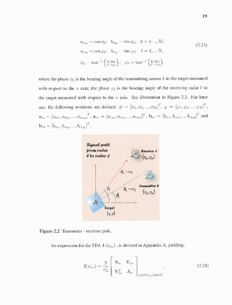
(2.23)
where the phase Ok is the bearing angle of the transmitting sensor k to the target measured
with respect to the x axis; the phase yok is the bearing angle of the receiving radar to
the target measured with respect to the x axis. See illustration in Figure 2.2. For later
use, the following notations are defined: = [01, 02, ..., 0/141T, = CO2, • • •, VNiT,
T Tatx -= [atx1, atx • • • , atam
i arx = [arxi 7 arX2 7 • • • ) arXN
]T 7 "ta: [biX1 btX2 7 • • • 7 btxmi
i
br, tbrxi brx2 , • • • , brxmiT •
Figure 2.2 Transmiter - receiver path.
An expression for the FIM J (072,) , is derived in Appendix A, yielding:
(2.24)

20
with the block matrices Sac, Aa, and V,,, terms defined in the Appendix A in (A.2), (A.3)-
(A.4) and (A.5)-(A.6) respectively.
In order to determine the value of J (O,), (2.15) and (2.21) are used in (2.24), to
obtain the following CRLB matrix:
(2.25)
The CRLB matrix is related to the sensor and target locations through the matrix H,
and to the received waveforms correlation functions and its derivatives through the Sn, and
V,„ matrices.
Orthogonal Waveforms When the waveforms are orthogonal, the block matrices Snc,
Aa, and V, simplify to (A.7) in Appendix A. This simplification enables to compute the
CRLB (2.25) in closed-form. This calculation is performed next.
While the CRLB expresses the lower bound on the variance of the estimate of Onc =
[x, y, ozR, al 7', only the estimation of x and y is of interest. The amplitude terms aR
and a' serve as nuisance parameters. For the variances of the estimates of x and y, it is
sufficient to derive the 2 x 2 upper left submatrix [CcRLB„e12x2 = [(J (Onc))-11 •2x2
The CRLB submatrix [CcRLBnel 2x2 for target localization in the noncoherent case
with orthogonal signals is:
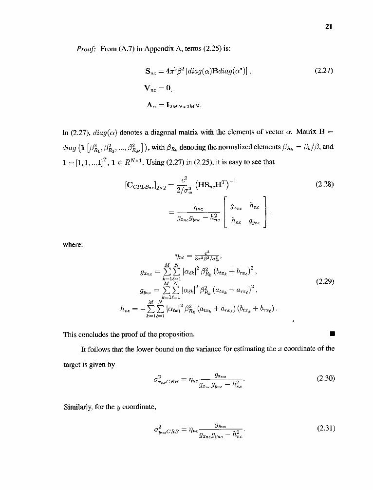
Proof: From (A.7) in Appendix A, terms (2.25) is:
21
(2.27)
(2.28)
(2.29)
This concludes the proof of the proposition. •
It follows that the lower bound on the variance for estimating the x coordinate of the
target is given by
(2.30)
Similarly, for the y coordinate,
(2.31)
22
The terms gx gv„c, and itn, are summations of atxk , arx„ btx, and brx, terms
that represent sine and cosine expressions of the angles çb and yo, and therefore relate
to the radars and target geometric layout. It is apparent that for the noncoherent case,
the lower bounds on the variances (2.30) and (2.31) are inversely proportional to the
averaged effective bandwidth 02, and SNR = 1/o (see expression for rm, in (2.29)).
It is interesting to note that i is actually the CRLB for range estimation in a single
antenna radar, based on the one-way time delay between the radar and the target (see for
example [26]). The other terms in (2.30) and (2.31) incorporate the effect of the sensor
locations.
2.3.2 Coherent Processing CRLB
Recall that in the signal model Section, the complex amplitude ail, i s associated with the
path transmitter k —÷ target —> receiver t. In the noncoherent case, the complex amplitude
is a nuisance parameter in estimating the target location x, y. In the coherent case, the
transmitting and receiving radars are assumed to be phase-synchronized. By eliminating
the phase offsets, the signal model in (2.8) applies, and the nuisance parameter role is left
to the complex target amplitude = CR + j(i. The coherent approach to localization seeks
to exploit the target location information embedded in the phase terms exp (-27rfc-rek) that
depend on the delays Tek, which in turn are function of the target coordinates x, y.
Define the vector of unknown parameters:
(2.32)
(2.33)

23
to be used in (2.15) to derive the CRLB. In comparing the coherent case in (2.33) with
the noncoherent counterpart in (2.18), note that 'on, incorporates the vectors aR and a1,
while 0, is a function of the scalars (R and (1- . The reduction in the number of unknown
parameters is made possible through the measurement of the phase terms of aR and a1.
For coherent observations, the conditional, joint pdf of the observations at the receive
sensors, given by (2.8), is of the form:
(2.34)
Following a process similar to the one in Section 2.3.1, the CRLB is derived for the
coherent case, based on the relation in (2.15). The matrix Pc takes the form:
(2.35)
where matrix H has the same form as in (2.22), since it is independent of the nuisance
parameters in both cases.
An expression for the FIN4 matrix, J (), is derived in Appendix B, yielding:
(2.36)
where the elements of the submatrices are found in Appendix B as follows: S, in (B.4).
in (B.5)-(A.5), and V, in (B.7)-(B.9).

24
The CRLB matrix for the coherent case is then found substituting (2.35) and (2.36)
in (2.15) and (2.14), obtaining:
-1
(2.37)
As in Section 2.3.1, the closed-form solution to the CRLB matrix in (2.37) is reduced
to the case of orthogonal waveforms. Since only the lower bound on the variances of the
estimates of x and y, is of interest, the submatrix [CcRLBc]2x2 RJ, (0)Y 2 x 2 is derived
and evaluated next.
Orthogonal Waveform The CRLB 2 x 2 submatrix for the coherent case and orthogonal
waveforms is:
(2.38)
Proof: From (B.11) in Appendix B the values of the matrices 5,, and V, are
obtained for orthogonal waveforms. Using this and H defined in (2.22) in (2.37), the CRLB
matrix CCRLB,, is obtained. Consequently, the submatrix [CcRLB,12x2 is computed,
resulting in the form given in (2.38).
This completes the proof of the proposition. •
From (2.38) and (B.11), it can be shown that [C CRLI3J2 x 2 can be expressed as:
(2.39)
25
where the various quantities are as follows:
(2.40)
The lower bound on the error variance is provided by the diagonal elements of the
[CeRLBcor] 2 x2 submatrix and are of the form:
(2.41)
The terms gxc, gw, and h, are summations of atx,, arx„ btxk and brxe that represent
sine and cosine expressions of the angles and cp, and therefore relate to the radars and
target geometric layout, multiplied by the ratio terms fR, = (1 + '374) . Invoking the
narrowband signals assumption i3W,2 < 1, it follows that fR, 1. These terms have
some additional elements when compared with the noncoherent case. It is apparent that
for the coherent case, the variances of the target location estimates in (2.41) are inversely
proportional to the carrier frequency p.
26
2.3.3 Discussion
The following observations are made:
• The lower bound on the variance in the noncoherent case is inversely proportional
to the averaged effective bandwidth For the coherent case, with narrowband
signals, where NI < 1, the localization accuracy is inversely proportional to the
carrier frequency .1', and independent of the signal individual effective bandwidth,
due to the use of the phase information across the different paths. It is apparent that
coherent processing offers a target localization precision gain (i.e., reduction of the
localization root mean-square error) of the order of fc/i3, refer to as coherency gain.
Designing the ratio f/ i3 to be in the range 100-1000, leads to dramatic gains.
• The term Tic in (2.40) is the range estimate based on one-way time delay with coherent
observations for a radar with a single antenna [53].
• The CRLB terms are strongly reliant on the relative geographical spread of the radar
systems vs. the target location. This dependency is incorporated in the terms a Xc 7
gynciye and lincie. It is apparent from (2.41), (2.30) and (2.31) that there is a trade-off
between the variances of the target location computed horizontally and vertically.
A set of sensor locations that minimizes the horizontal error, may result in a high
vertical error. For example, spreading the transmitting and receiving radars in an
angular range of — (ir /10) to -I- (7/10) radians with respect to the target, will result
in high horizontal error while providing low vertical error, as intuitively expected.
This is caused by the fact that the terms gx„,c/gxe are summations of sine functions
and gy„c /gye are summation of cosine functions of the same set of angles. In order to
truly determine the minimum achievable localization accuracy in both x and y axis,
the over-all accuracy, defined as the total variance a! = (\crx2ecRB ay2eCRB) needs
to be minimized.
27
• The message of dramatic improvement in localization accuracy needs to be
moderated with the observation that the CRLB is a bound of small errors. As such,
it ignores effects that could lead to large errors. For example, MINIO radar with
distributed sensors and coherent observations is subject to high sidelobes [1]. These
topics are outside the scope of this paper, but they should be kept in perspective.
• Phase synchronization: The coherent scheme promises of higher accuracy
performances involve the challenge of distributed carrier phase synchronization.
The synchronization complexity in distributed and autonomous sensors/platforms
is common to widely spread MIMO radar systems, wireless sensor networks and
cooperative wireless communication. In the latter two, some of the proposed
solutions make use of a reference signal [54-57] provided by one of the sensors.
These schemes mainly focus on master/slave strategies where one sensor is chosen
to be the master and broadcasts a sinusoidal reference signal to all slaves. Carrier
phase synchronization is also established using an external beacon in the form of a
GPS or a ground communication broadcasting station [58-61]. These highly stable
broadcasting sources continuously transmit a reference signal to be used at each
sensor node, where more than one beacon may be used for higher accuracy. In
all of these synchronization methods, a periodic re-synchronization is necessary to
avoid unacceptable levels of phase drift. The increasing interest in distributed phase
synchronization and vibrant research activity set the ground for promising progress.
• Doppler shift: The CRLB on target localization is developed for a stationary target
whereas the CRLB on target velocity estimation is developed in [50]. Consequently,
the model in (2.8) does not account for Doppler frequency. In practice, a Doppler
shift might be introduced and affect the estimation performance with coherent
processing. To evaluate the affect of such a Doppler shift on the CRLB the following

28
signal model adaptation is applied [31]:
where fda is the Doppler frequency and it- < 1 is assumed. Without loss of
generality, the transmitted waveforms are time-delayed such that they add coherently
in the center of a given search cell [o 1J . For a slow moving target, i.e.
< 1, the Doppler term exp (j21rfd,kt) P.:: 1 and therefore the Doppler shift
does not affect the localization performance as shown in this section. If the latter
does not apply, the off-diagonal elements of matrix S, are non-zero and therefore
introduce an estimation error. A current research effort is focused on the extension
of the current model to a Bayesian CRLB that accounts for both target location and
velocity estimation.
• Orthogonality: The CRLB is developed for a general set of waveforms {sk (t)}. The
general solution in (2.25) and (2.37) is later given in closed-form for the special case
of orthogonal signals. Albeit the design of such signal sets is beyond the framework
of this paper, elaboration as for some possible schemes is provided. Attaining a set of
orthogonal waveforms that follow the requirement of f sk (v) s, (ii — ATek,w)
0 over all cross-elements, k k', and any Ara,,ek, = Tew , is a challenging
task. Accomplishing full orthogonality under these conditions is very demanding.
A practical way to address this problem is by relaxing the design criteria to low
cross-correlation, i.e., If sk (v) s, — ATtkrek,) dv I < 6, where € is chosen such
that the estimation MSE performance penalty, with respect to fully orthogonal sets,
in minimized. This offers a reasonable way to generate approximate-orthogonal
waveforms for some range of delays or what is defined in [62] as quasi-orthogonal
waveforms. Such an alternative is presented in [50]. Some other design possibilities
are provided in [21-23,62]. The extension of the radar AF to the MlMO radar case
in [24,25] offers design tools for such quasi-orthogonal waveforms. The CRLB

29
analytical expressions provided in Appendix A and Appendix B could than be used
for a comparative evaluation of the CRLB performance for a given quasi-orthogonal
set vs. a fully orthogonal set of waveforms.
• The lower bound as expressed by the CRLB, provides a tight bound at high SNR,
while at low SNR, the CRLB is not tight [28]. As the ambiguity problems are usually
addressed through the signal waveform design, a more rigid bound needs to be found
for the localization variance in the low-SNR case.
The coherency gain obtained with coherent processing makes it advantageous over
noncoherent processing. All the same, the contribution of the product terms gxe, gm and
h, needs further evaluation. The following sections focus on elucidating the role of these
terms for coherent processing.
2.4 Effect of Sensor Locations
The CRLB for target localization with coherent MIMO radar shows a gain, i.e., reduction
in the standard deviation of the localization estimate, of MO compared to noncoherent
localization. Yet, the CRLB is strongly dependent on the locations of the transmitting and
receiving sensors relative to the target location, through the terms gxlx„ gynelue and kick.
To gain a better understanding of these relations, and set a lower bound on the CRLB over
all possible sensor placements, further analysis is developed in this section.
The following general notation are introduced: for any given set of vectors e =
(2.43)
30
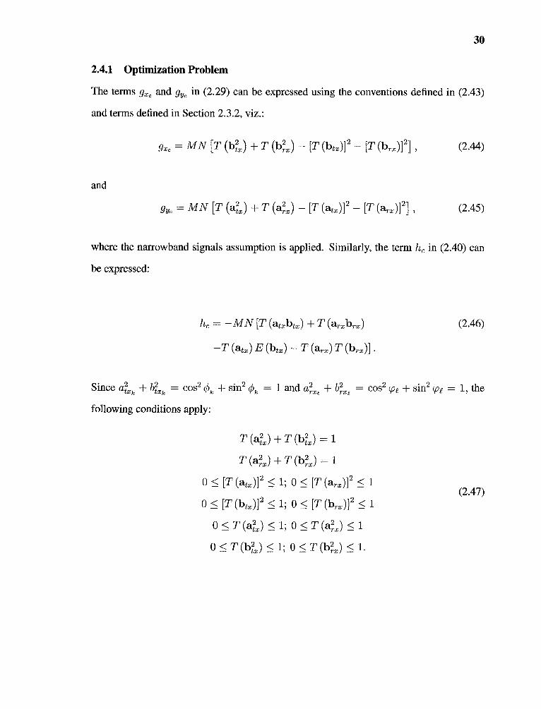
2.4.1 Optimization Problem
The terms gxe and gye in (2.29) can be expressed using the conventions defined in (2.43)
and terms defined in Section 2.3.2, viz.:
(2.44)
(2.45)
where the narrowband signals assumption is applied. Similarly, the term he in (2.40) can
be expressed:
(2.46)
(2.47)

31
Seeking to find sets of angles 0* and (p*, that yield sets of cosine and sine expressions
a'tKx, ars`x, bt*x,13,*x for which the values of the Cramer-Rao bounds for localization along the
x and y axes (crLCRB and Cry2cCRB7 respectively) are jointly minimized,
(2.48)
This is equivalent to minimizing the trace of the CRLB submatrix [CcRLBe] 2x2• The
explicit minimization problem is formulated introducing the objective function fo:
(2.49)
This representation of the problem is not a convex optimization problem.' The next
steps are undertaken in order to formulate a convex optimization problem equivalent to
(2.49), i.e., a convex optimization problem that can be solved through routine techniques
and from whose solution it is readily possible to find the solution to (2.49).
In [39], it is shown that for a given positive definite matrix, in our case [CcRLse]2x2,
and its inverse matrix F, in this case:
(2.50)
the following relation exists between the diagonal elements of these matrices:
(2.51)
"A convex optimization problem in standard form is [63]
minimizesubject to
for some constants az, i, j, i 1, ..., m, j 1, ...,p, and where fo, fm are convex functions.
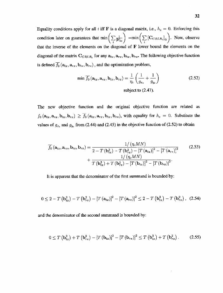
32
Equality conditions apply for all i if F is a diagonal matrix, i.e., lic = 0. Enforcing this
condition later on guarantees that min ( E[Fh- =min E [CcRLBJ,ii •
Now, observe
that the inverse of the elements on the diagonal of F lower bound the elements on the
diagonal of the matrix CCRLBc for any atx, arx, btx , brx. The following objective function
is defined fo (atm, a,, btx,brx) , and the optimization problem,
(2.52)
The new objective function and the original objective function are related as
fo (at, arx ,b-tx,brx) fo (at., arx,btx,brx), with equality for h = 0. Substitute the
values of gxc and gye from (2.44) and (2.45) in the objective function of (2.52) to obtain
(2.53)
It is apparent that the denominator of the first summand is bounded by:
(2.54)
and the denominator of the second summand is bounded by:
(2.55)

33
Denote T (bL) T (13,2x) = p, and let T (atm) = T (arx) = T (btx) = T (brx) = 0. Then,
from (2.53)-(2.55) and (2.52), the following problem is obtained:
(2.56)
The objective function A (m) = p(22 is convex since g(t) = ,u,(2 — p,) is a concave
function and A (it) = h (g(p)) = *)9 is a convex and nondecreasing function [63]. The
inequality constraint functions are convex as well. Therefore, the problem described in
(2.56) is a convex optimization problem. The epigraph form is a way to introduce a
linear (and convex) objective t, while the original objective fo is incorporated into a new
constraint fo — t < 0 [63]. The key point here is that the inequality constraint function
A — t < 0 can be transformed to a linear convex form [64].
An equivalent epigraph form of the convex optimization problem given in (2.56)
may be expressed by using two variables, t1 and t2, after rewriting the objective function as1 1
fo (A) = foi Cu) + fo2 (it), where foi (it) = 2 — and fo2 (p) = —. Two new inequality p,
constraint functions are introduced: 1
ti < 0 and —1 — t2 < 0. After some simple
2 — p,algebraic manipulations, the epigraph form turns into the following convex optimization
problem:
(2.57)

34
A convenient way to solve this convex optimization problem is to employ the
concept of Lagrange duality and exploit the sufficiency of the Karush-Kuhn-Tucker (KKT)
conditions [63]. The Lagrangian of the problem in (2.57) is given by:
The KKT conditions state that the optimal solution for the primal problem
(minimization of t 1 + t2 in (2.57)) is given by the solution to the set of equations:
(2.59)
Applied to (2.57) and (2.58), these equations specialize to
35
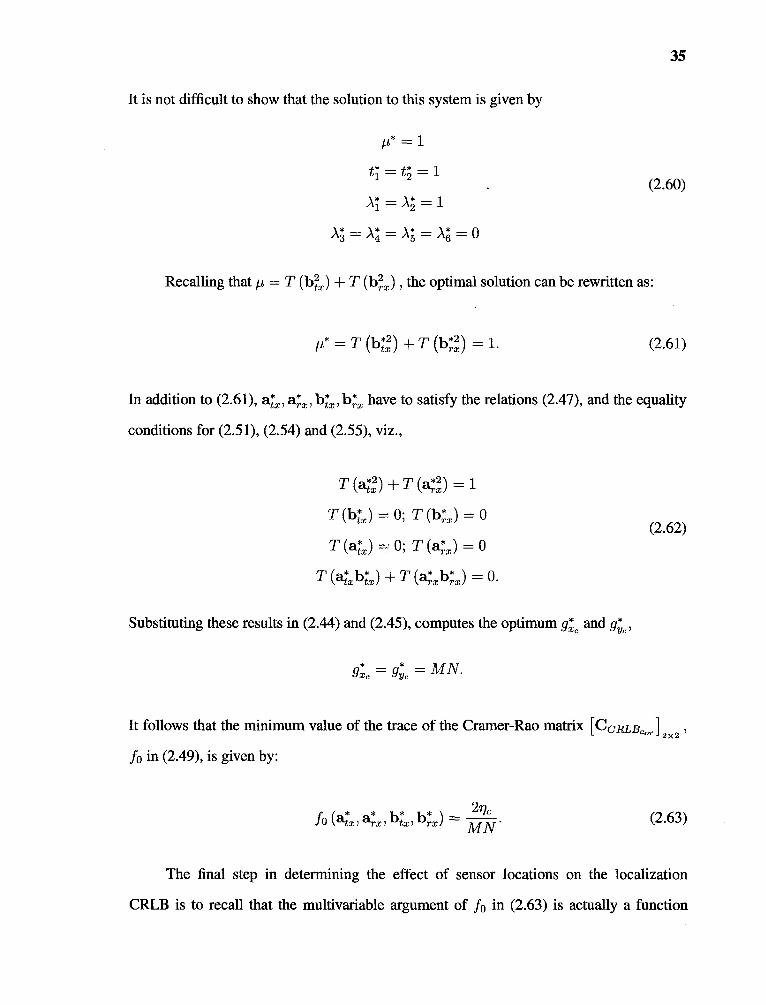
It is not difficult to show that the solution to this system is given by
(2.60)
Recalling that ft= T (bL) + T (b2,x) , the optimal solution can be rewritten as:
(2.61)
In addition to (2.61), ast's , a;:x, bikx, lc•;:x have to satisfy the relations (2.47), and the equality
conditions for (2.51), (2.54) and (2.55), viz.,
(2.62)
Substituting these results in (2.44) and (2.45), computes the optimum gx*e and gy%,
It follows that the minimum value of the trace of the Cramer-Rao matrix [CcRLBcor]2x2
fo in (2.49), is given by:
(2.63)
The final step in determining the effect of sensor locations on the localization
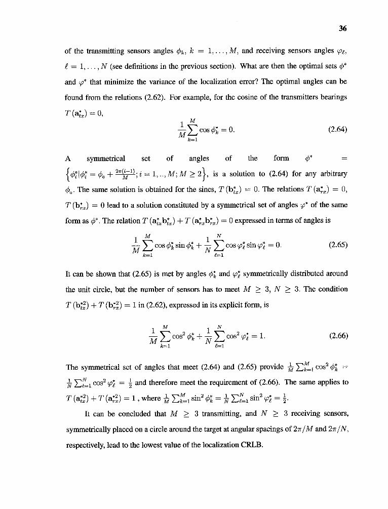
CRLB is to recall that the multivariable argument of fo in (2.63) is actually a function
36
of the transmitting sensors angles ok, k = 1, . . . , M, and receiving sensors angles (pe,
t -= 1, . .. , N (see definitions in the previous section). What are then the optimal sets 0*
and (p* that minimize the variance of the localization error? The optimal angles can be
found from the relations (2.62). For example, for the cosine of the transmitters bearings
T (aL) = 0,
(2.64)
A symmetrical set of angles of the form 0*
{0'1195; = sçbo + 214mi-1) ; i = 1, M; M > 21, is a solution to (2.64) for any arbitrary
O.. The same solution is obtained for the sines, T (blx) = 0. The relations T (a;s) = 0,
T (14x) = 0 lead to a solution constituted by a symmetrical set of angles (p* of the same
form as 0*. The relation T (aLlYtkx) + T (abr* x) --= 0 expressed in terms of angles is
(2.65)
It can be shown that (2.65) is met by angles 0;`, and (p; symmetrically distributed around
the unit circle, but the number of sensors has to meet M > 3, N > 3. The condition
T (bg) + T (bg) = 1 in (2.62), expressed in its explicit form, is
(2.66)
The symmetrical set of angles that meet (2.64) and (2.65) provide -ml EkM COS2 q5
cos2 c,07, = and therefore meet the requirement of (2.66). The same applies to
T (ag) + T (ag) = 1 , where b- EkM sin2 = -k- EtN sin2 (p; =
It can be concluded that M > 3 transmitting, and N > 3 receiving sensors,
symmetrically placed on a circle around the target at angular spacings of 27/M and 27/N,
respectively, lead to the lowest value of the localization CRLB.
37
This result can be extended by noticing that relations (2.62) also hold for any
superposition of symmetrical sets containing no less than 3 transmitting and/or receiving
sensors. Therefore, the complete set of optimal points is given by:
(2.67)
where the total number of transmitting (M) and receiving (N) radars may be divided
into V and U sets of symmetrically placed radars, each set consists of Z, and 4, radars,
respectively. The angles 0,, and (p„ are an initial arbitrary rotation of the symmetric sets Zu
and Zu, correspondingly.
As a special case, it is interesting to evaluate the CRLB in (2.39) with 1 transmitter
and MN receivers, i.e., a Single-Input Multiple-Output (SIMO) system. This scheme
makes use of (MN + 1) radars instead of (M N) radars used in a MIMO system with
M transmitters and N receivers. From (2.67) it is apparent the this case does not provide
optimality since the number of transmitters is smaller than 3. To evaluate cqeCRB ± CY y2 ,CRB
for this setting assume 1 transmitter is located at an arbitrary angle 0, with respect to the
target, and a set of MN receivers are located symmetrically around the target, at angles (p*
that follow the condition in (2.67). The expressions in (2.44), (2.45), and (2.46) reduce to
the form:
(2.68)

38
and the trace of the CRLB submatrix [CcRLBJ2x2, defined by fo (atm, arx btx, brx) =
(2.69)
This result expresses an increase in the estimation error by a factor of 2 when compared
with M transmitters and N receivers given in (2.63).
2.4.2 Discussion
The following comments are intended to provide further insight into the results obtained in
this section.
• From (2.63), the lowest CRLB for target localization utilizing phase information is
given by 277,1 (MN). The reduction in the CRLB by the factor MN/2 compared to a
single antenna range estimation given by, tic ia referred as a M/MO radar gain. This
gain reflects two effects: (1) the gain due to the system footprint; (2) the advantage
of using M transmitters and N receivers, rather than, for example, 1 transmitter and
MN receivers. The latter gain is apparent when M N >> (M + N).
• The CRLB obtained through the use of a single transmit antenna and MN receive
antennas in (2.69) is 470 (MN). It follows that MIMO radar, with a total of M + N
sensors, has twice the performance (from the point of view of localization CRLB) of
a system with a single transmit antenna and MN receive antennas.
• The best accuracy is obtained when the transmitting and receiving radars are located
on a virtual circle, centered at the target position, with uniform angular spacings of
27-/M and 27r/N, respectively, or any superposition of such sets.
• The optimization analysis presented in this section is intended to provide insight
into the effect the sensor locations have on the CRLB. Naturally, in practice, it
is not possible to control in real time the location of the sensors relative to a
39
target. However, the results here teach us that selecting among the sensors those
who are most symmetrical with respect to the target may lead to the most accurate
localization.
So far the focus was on the theoretical lower bound of the localization error. In the
next section, specific techniques for target localization and their performance as a function
of sensor locations are discussed. For this purpose, the GDOP metric and GDOP contour
mapping tools are introduced.

CHAPTER 3
METHODS FOR TARGET LOCALIZATION
The lower bound on the variance of target localization estimate was formulated in Chapter
2. The MLE [65], developed in [18], does not lend itself to a closed-form expression,
and numerical methods need to be used to solve it. A closed-form solution to the target
localization can be obtained by application of the BLUE. The later, allows the use of the
GDOP metric for a more comprehensive understanding of the relation between the target
and the sensor locations.
3.1 BLUE for Noncoherent and Coherent Target Localization
To formulate the BLUE, it is necessary to have an observation model in which observations
change linearly with the target location coordinates. That is because it is inherent to the
BLUE that the estimate is linear. To this end, a model is formulated in which the time
delays are "observable." In practice, the time delays are not directly observable. Rather,
they are estimated, for example by maximum likelihood, from the received signals. Then,
the term cm is the time delay estimation error. Our BLUE estimation problem of the target
location should not be confused with the estimation of the time delays. The estimation
of the time delays is just a preparatory step in setting up the "observations" of the BLUE
model. Once, the observation model has been set up, it is necessary to ensure that the
model between the time delays and target location is linear. Setting the origin of the
coordinate system at some nominal estimate of the target location X, ---= (xe, ye) and
preserving only linear terms of the Taylor expansion of expressions such as in (2.9), the
time delays introduced by a target may be introduced as linear functions of x and y,
40
41
where the angles Cbk and çoi are the bearings that the transmitting sensor k and receiving
sensor .e, respectively, subtend with the reference axis (with the origin at the nominal
estimate of the target location). The vertex of the angles is an arbitrary point in the
neighborhood of the true target location.
The linear model may be simplified as,
(3.2)
Let the observed time delay associated with a transmitter-receiver pair be pa, then
(3.3)
where ea is the "observation noise." The following linear model is postulated between the
observable time delays fi = [P11) ii-t127 -.-1 ANM]T and the vector of unknown parameters 0:
(3.4)
where the matrix D defined the linear relation between F- and the vector of unknowns 0.
The vector € = [ca, En, • • • , EArmlT is the MN x 1 measurement noise vector. According to
(3.4), the BLUE's "observations" are in the form of time delays. So an intermediate step
of time delay estimation is implied.
For the linear and Gaussian model in (3.4), the BLUE is computed from the
Gauss-Markov theorem [26] that states the BLUE of the unknown vector 0 is given by
the expression:
(3.5)
where C, is the covariance matrix characterizing the "noise" terms Ea •
42
The theorem also determines the error covariance matrix for the estimator "O' „„ to
be
(3.6)
From this point onward, the BLUE is developed for the case of noncoherent and
coherent processing, separately.
3.1.1 BLUE for Noncoherent Processing
Recall that in signal model Section, the complex amplitude aek associated with the path
transmitter k -4 target —> receiver .e in the received signal model given in (2.10) was
defined. In the noncoherent case, the complex amplitude is a nuisance parameter in
estimating the target location x, y. There is no common phase reference among the sensors
and phase information is not exploited in the estimation process. Consequently, the time
observation, evaluated using noncoherent processing, are not affected by phase/time bias.
In this case, the vector of unknown parameters is defined as On, = [x, yr and the the time
measurements are modeled as:
(3.7)
The relation in (3.7) can be written as:
(3.8)
43
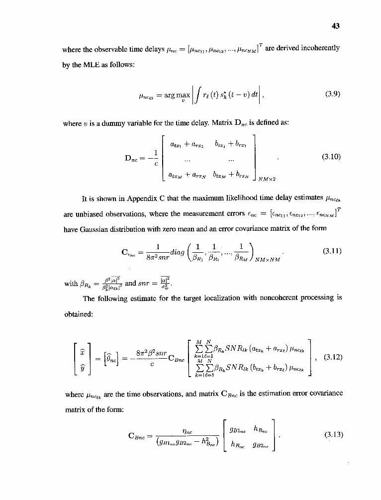
where the observable time delays Anc = [ji,, Anci2 itneNmiT are derived incoherently
by the MLE as follows:
(3.9)
where v is a dummy variable for the time delay. Matrix Dne is defined as:
(3.10)
It is shown in Appendix C that the maximum likelihood time delay estimates ttnctk
are unbiased observations, where the measurement errors cnc = frL-nen Cnc12, • ••, EncArmiT
have Gaussian distribution with zero mean and an error covariance matrix of the form
(3.11)
021_12 d lap
With /3Ak ;Z:k112 ail snr •a
The following estimate for the target localization with noncoherent processing is
obtained:
(3.12)
•■•
where tincek are the time observations, and matrix CBn, is the estimation error covariance
matrix of the form:
(3.13)

44
and
(3.14)
Using these results in (3.13) provides the MSE for the BLUE as follows:
(3.15)
for the estimation of the x coordinate, and
(3.16)
for the estimation of the y coordinate.
3.1.2 BLUE for Coherent Processing
In the coherent case, the transmitting and receiving radars are assumed to be both time
and phase-synchronized. The target reflectivity parameter rc exp (j2R-Oc), results in a
common unknown time delay nuisance parameter A, = fc for the signal model given
in (2.8), where is replaced by rc exp (j2T-LAT). The time delay observations in coherent
MIMO radars are therefore of the form:
(3.17)
where the vector of unknowns is 0, = [x, y, 6,]T. The linear observation model is
represented through:
(3.18)
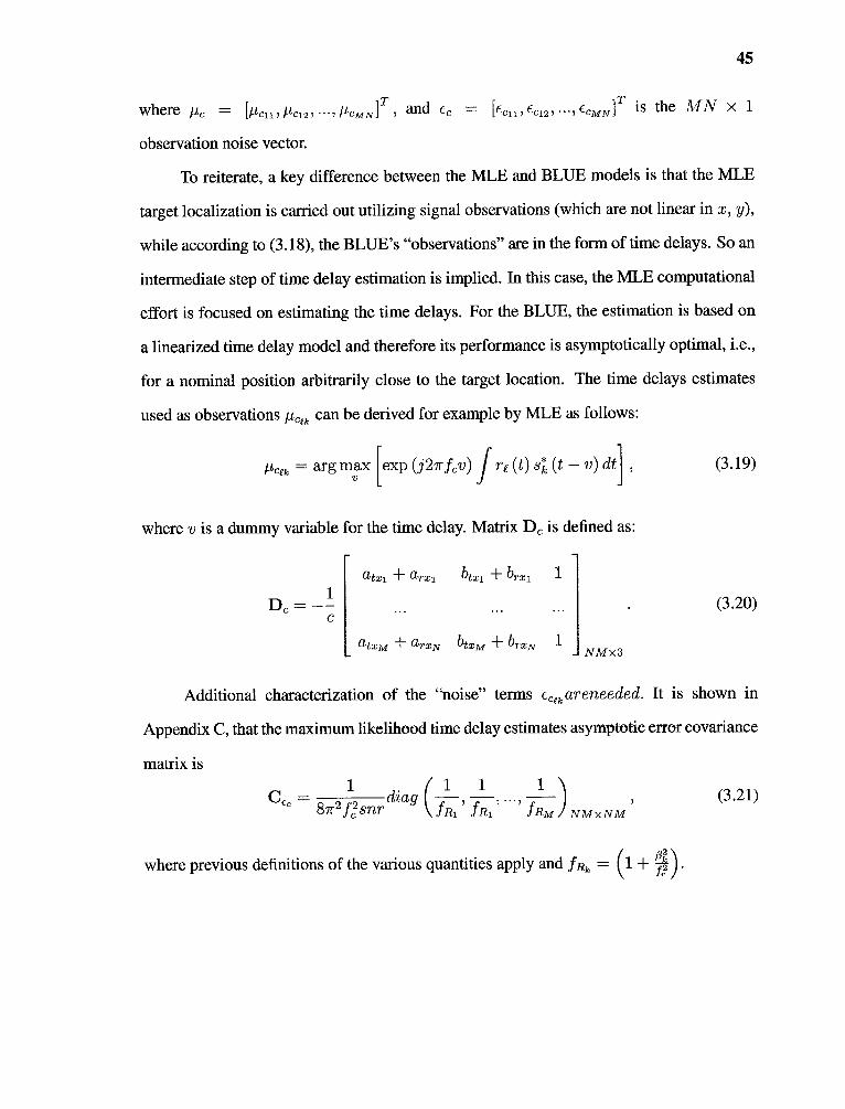
45
where ,C [µc11, PC121 ' • 7 PcmiviT 7 and cc [(cu. cci2, • • • , €cmN1T is the AI N x 1
observation noise vector.
To reiterate, a key difference between the MLE and BLUE models is that the MLE
target localization is carried out utilizing signal observations (which are not linear in x, y),
while according to (3.18), the BLUE's "observations" are in the form of time delays. So an
intermediate step of time delay estimation is implied. In this case, the MLE computational
effort is focused on estimating the time delays. For the BLUE, the estimation is based on
a linearized time delay model and therefore its performance is asymptotically optimal, i.e.,
for a nominal position arbitrarily close to the target location. The time delays estimates
used as observations ti,„, can be derived for example by MLE as follows:
(3.19)
where v is a dummy variable for the time delay. Matrix D, is defined as:
(3.20)
Additional characterization of the "noise" terms c„,areneeded. It is shown in
Appendix C, that the maximum likelihood time delay estimates asymptotic error covariance
matrix is
(3.21)
R2where previous definitions of the various quantities apply and fR, = (1 +
) •

...,
46
Using the time error covariance matrix C,c and the linear transformation matrix D in
(3.20), the following estimate for -613 is obtained:
(3.22)
The error covariance matrix for (x, -#) is derived using (3.20) and (3.21) in (3.22) and
calculating the 2 x 2 upper left submatrix, resulting with
(3.23)
The elements of matrix GB are:
(3.24)
arze) (btxk ± brxe))
Using these results in (3.23) provides the MSE for the BLUE as follows:
(3.25)
for the estimation of the x coordinate, and
(3.26)

47
for the estimation of the y coordinate.
3.1.3 Discussion
The following points are worth noting:
• The BLUE estimator are provided in closed-form for coherent and noncoherent
processing. This allows for an analytical analysis of the MSE performance using the
GDOP metric that presents a performance study tool for a given layout of sensors.
Nonetheless, it does not eliminate the complex computational effort involved in the
intermediate step of time delays estimation.
• In general, the variances (3.15), (3.16), (3.25) and (3.26) have similar functional
dependencies on the carrier frequency and on the sensor deployment as the CRLB.
The terms atx, arxe, btxk and brxe embedded in (3.14) and (3.24) relate the sensors
layout to the variance of the BLUE.
• For a target located arbitrarily close to the nominal position, the linearization error
is negligible and the bearing angles of the transmit and receive radars, with respect
to the target and the nominal position, are approximately the same. In this case,
the BLUE performance is determined by the asymptotic characteristics of the time
delays estimates used as observations, and derived by the MLE in (3.11) and (3.21).
In [66, 67], MLE of the time delays is shown to approach the CRLB arbitrarily close
at high-SNR. In this region, the time delays estimation error asymptotic covariance
matrices, given by (3.11) and (3.21), are valid. Consequently, the BLUE estimator
coefficients, gsincic, gB2nc/c, and hs in (3.14) and (3.24), approximate the CRLB
terms given in Chapter (2), Section (2.3), and the BLUE asymptotically reach the
CRLB.
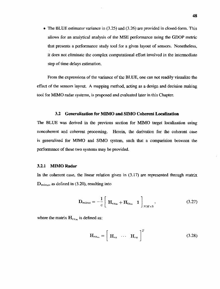
48
• The BLUE estimator variance in (3.25) and (3.26) are provided in closed-form. This
allows for an analytical analysis of the MSE performance using the GDOP metric
that presents a performance study tool for a given layout of sensors. Nonetheless,
it does not eliminate the complex computational effort involved in the intermediate
step of time delays estimation.
From the expressions of the variance of the BLUE, one can not readily visualize the
effect of the sensors layout. A mapping method, acting as a design and decision making
tool for MIMO radar systems, is proposed and evaluated later in this Chapter.
3.2 Generalization for MINI° and SIMO Coherent Localization
The BLUE was derived in the previous section for MIMO target localization using
noncoherent and coherent processing. Herein, the derivation for the coherent case
is generalized for MIMO and SIM° system, such that a comparision between the
performance of these two systems may be provided.
3.2.1 MIMO Radar
In the coherent case, the linear relation given in (3.17) are represented through matrix
Dminio, as defined in (3.20), resulting into
(3.27)
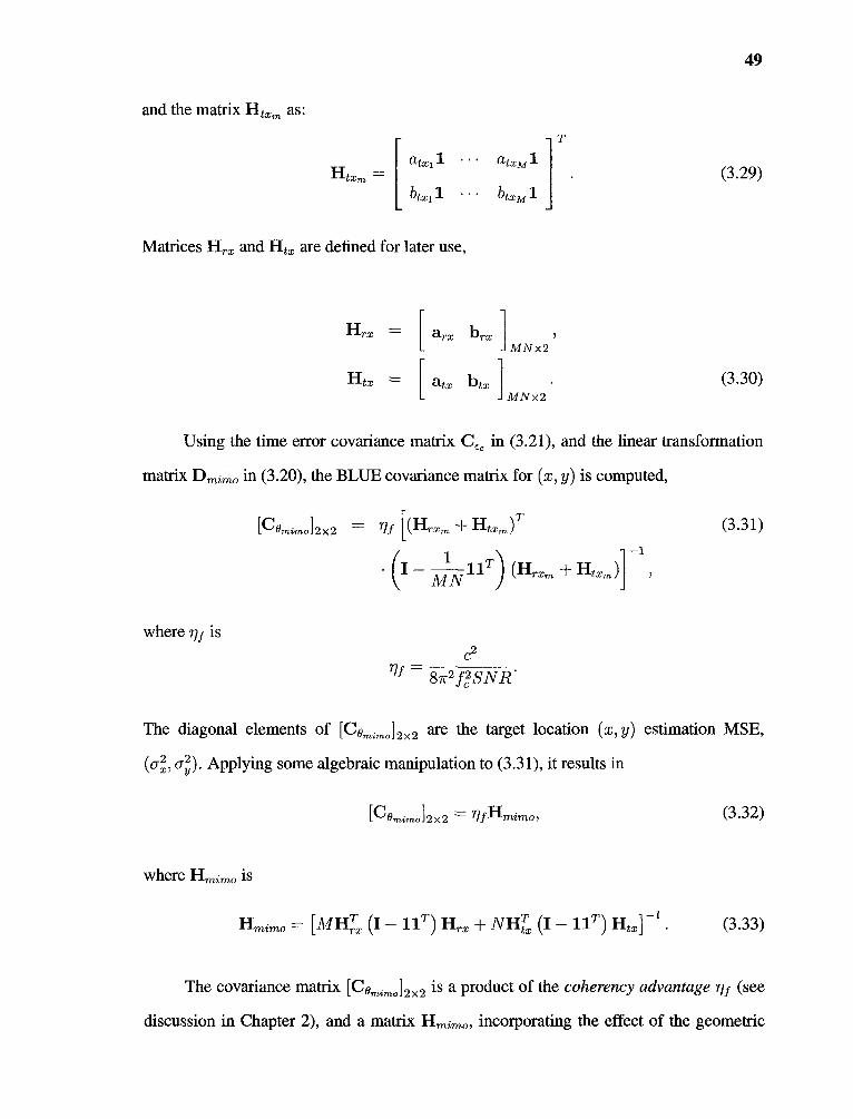
49
and the matrix Ht, as:
(3.29)
Matrices Hrx and Htx are defined for later use,
(3.30)
Using the time error covariance matrix C,c in (3.21), and the linear transformation
matrix Dminw in (3.20), the BLUE covariance matrix for (x, y) is computed,
(3.31)
The diagonal elements of [Cθmimo]2 x2 are the target location (x, y) estimation MSE,(ux2, ) Applying some algebraic manipulation to (3.31), it results in
(3.32)
(3.33)
The covariance matrix [Cθmimo]2 x 2 is a product of the coherency advantage nf (see
discussion in Chapter 2), and a matrix Hmirnol incorporating the effect of the geometric
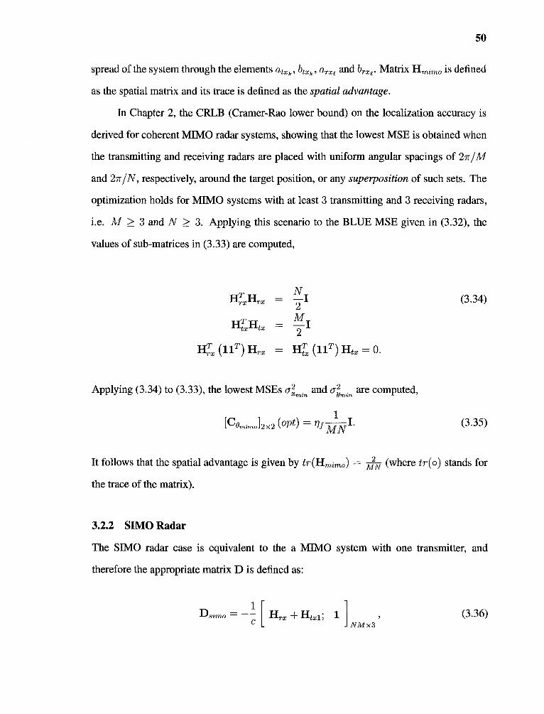
50
spread of the system through the elements atxk, btx,, arx, and brx,. Matrix 1.197,,,,„ is defined
as the spatial matrix and its trace is defined as the spatial advantage.
In Chapter 2, the CRLB (Cramer-Rao lower bound) on the localization accuracy is
derived for coherent MIMO radar systems, showing that the lowest MSE is obtained when
the transmitting and receiving radars are placed with uniform angular spacings of 27r/M
and 27/N, respectively, around the target position, or any superposition of such sets. The
optimization holds for MIMO systems with at least 3 transmitting and 3 receiving radars,
i.e. M > 3 and N > 3. Applying this scenario to the BLUE MSE given in (3.32), the
values of sub-matrices in (3.33) are computed,
(3.34)
Applying (3.34) to (3.33), the lowest MSEs o-LiTh and aLm are computed,
(3.35)
It follows that the spatial advantage is given by tr(1-1,,,,,o) Tj-N- (where tr(o) stands for
the trace of the matrix).
3.2.2 SIMO Radar
The SIMO radar case is equivalent to the a MIMO system with one transmitter, and
therefore the appropriate matrix D is defined as:
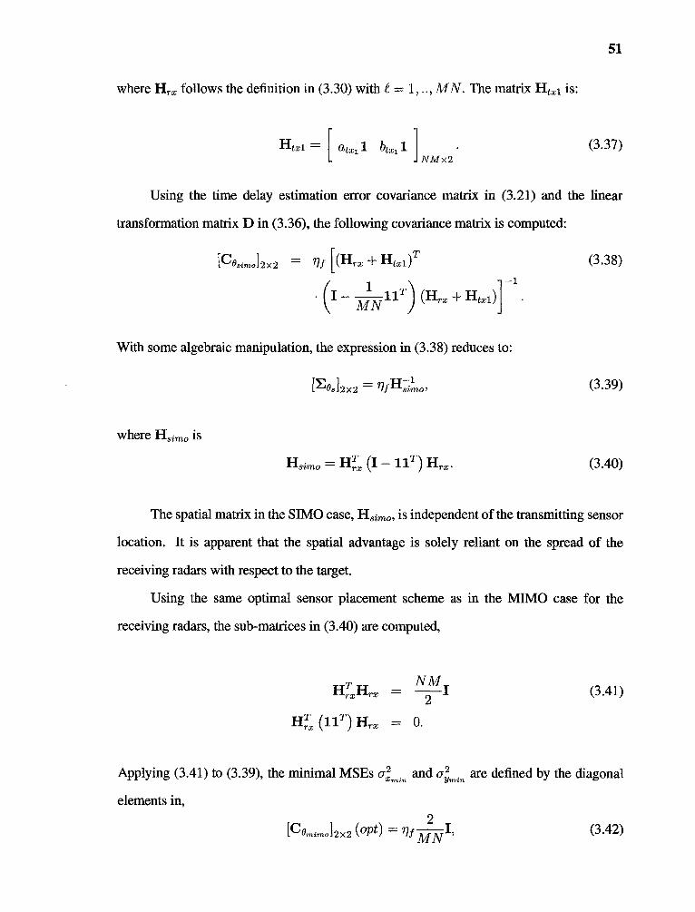
51
where Hrx follows the definition in (3.30) with =1, .., MN. The matrix Iltx1 is:
(3.37)
Using the time delay estimation error covariance matrix in (3.21) and the linear
transformation matrix D in (3.36), the following covariance matrix is computed:
(3.38)
With some algebraic manipulation, the expression in (3.38) reduces to:
(3.39)
(3.40)
The spatial matrix in the &IMO case, lisimo, is independent of the transmitting sensor
location. It is apparent that the spatial advantage is solely reliant on the spread of the
receiving radars with respect to the target.
Using the same optimal sensor placement scheme as in the MIMO case for the
receiving radars, the sub-matrices in (3.40) are computed,
(3.41)
Applying (3.41) to (3.39), the minimal MSEs σ²ymin are defined by the diagonal
elements in,
(3.42)

52
offering a spatial advantage of tr(lisin,„) =
3.2.3 Discussion
The covariance matrix for the target localization was derived, and the minimal MSEs were
calculated and given in (3.35) and (3.42). The following features of coherent MIMO and
SIMO localization are worth noting:
• The spatial advantage is determined by the footprint of the multiple sensor system
relative to the target location. A MlMO system with M > 3 transmitters and
N> 3 receivers, positioned optimally with respect to the target, has twice the spatial
advantage of a SIMO system with 1 transmitter and MN receivers.
• The MIMO system has a considerable advantage by employing K =-- M+N sensors,
whereas the SIMO system employs K = (MN -I- 1) sensors. This gain becomes
significant for a large number of sensors, where (M + N) < MN.
The effect of the sensors and the target positions on the expressions in (3.32) and
(3.39) for other than optimal setting cannot be intuitively identified. A more suitable
method to express these relations is employed in the next section. These evaluation tools
incorporate the mapping of spatial advantage over a given geographical area, using the
GDOP metric.
3.3 GDOP
In Chapter 2 Section 2.4, optimal sensor location that minimize the CRLB was discussed
. In practice, radars deployment is a given one. The question si - what is the localization
accuracy performance of an existing radars spread and a specific target location? GDOP
is a metric that addresses this question. The GDOP is commonly used in GPS systems for
mapping the attainable localization accuracy for a given layout of GPS satellites positions

53
[39, 40]. The GDOP metric emphasizes the effect of sensor locations by normalizing the
localization error with the term contributed by the range estimate.
3.3.1 GDOP for MIMO
The GDOP metric is commonly defined as:
(3.43)
where a2 is the range (delay) measurements error, defined by standard deviation of the
time delays c2al. cov (X), where cov (0) stands for the covariance matrix. For the two
dimensional case, where X = (x, y), it is:
(3.44)
where ax2 and ay2 are the variances of localization on the x and y axis, respectively. A one
dimensional metric is defined: the horizontal x-axis DOP (HxDOP) and horizontal y-axis
DOP (HyDOP), as:
(3.45)
(3.46)
The BLUE MSEs given in (3.15), (3.16), (3.25) and (3.26), are used together with the
time delay variances in (3.11) and (3.21), to evaluate the GDOP metric for MIMO radar
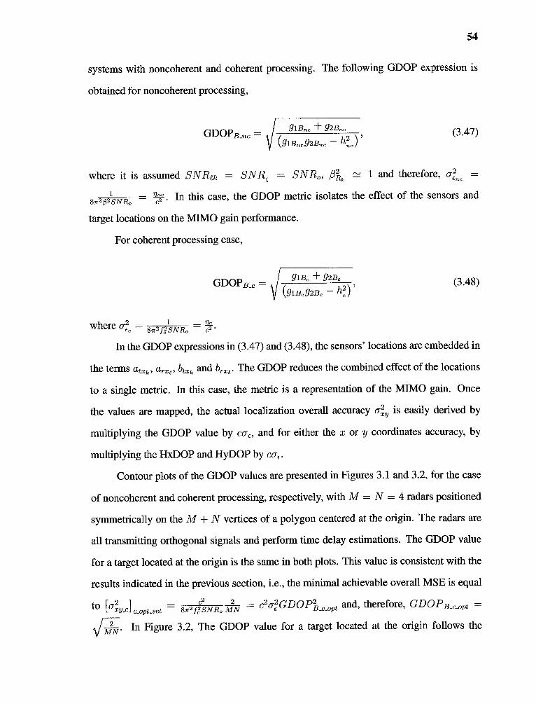
54
systems with noncoherent and coherent processing. The following GDOP expression is
obtained for noncoherent processing,
(3.47)
where it is assumed SNRek = SNRc = SNRo, β²R β²Rk and therefore, cr,2 =
8π²β²SNRo = • In this case, the GDOP metric isolates the effect of the sensors and
β² c²
target locations on the MIMO gain performance.
For coherent processing case,
(3.48)
where o-f2c = 87r2f21SNRo = •
In the GDOP expressions in (3.47) and (3.48), the sensors' locations are embedded in
the terms at,k , arxt, btxk and brx,. The GDOP reduces the combined effect of the locations
to a single metric. In this case, the metric is a representation of the MIMO gain. Once
the values are mapped, the actual localization overall accuracy ax2y is easily derived by
multiplying the GDOP value by ca„ and for either the x or y coordinates accuracy, by
multiplying the HxDOP and HyDOP by cut.
Contour plots of the GDOP values are presented in Figures 3.1 and 3.2, for the case
of noncoherent and coherent processing, respectively, with M = N = 4 radars positioned
symmetrically on the M N vertices of a polygon centered at the origin. The radars are
all transmitting orthogonal signals and perform time delay estimations. The GDOP value
for a target located at the origin is the same in both plots. This value is consistent with the
results indicated in the previous section, i.e., the minimal achievable overall MSE is equal
to 2/MN c²σ²eGDOP²B_c_opt and, therefore, GDOPB_c_opt =[σ²xy,c] c_opt_set = 8π²f²SNRo
6-712-17. In Figure 3.2, The GDOP value for a target located at the origin follows the
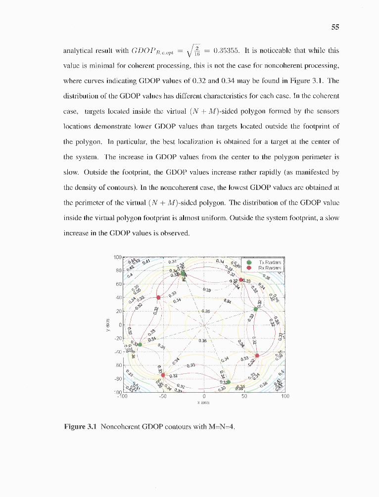
55
analytical result with GDOPB_c_opt = = 0.35355. It is noticeable that while this
value is minimal for coherent processing, this is not the case for noncoherent processing,
where curves indicating GDOP values of 0.32 and 0.34 may be found in Figure 3.1. The
distribution of the GDOP values has different characteristics for each case. In the coherent
case, targets located inside the virtual (N + M)-sided polygon formed by the sensors
locations demonstrate lower GDOP values than targets located outside the footprint of
the polygon. In particular, the best localization is obtained for a target at the center of
the system. The increase in GDOP values from the center to the polygon perimeter is
slow. Outside the footprint, the GDOP values increase rather rapidly (as manifested by
the density of contours). In the noncoherent case, the lowest GDOP values are obtained at
the perimeter of the virtual (N + M)-sided polygon. The distribution of the GDOP value
inside the virtual polygon footprint is almost uniform. Outside the system footprint, a slow
increase in the GDOP values is observed.
Figure 3.1 Noncoherent GDOP contours with M=N=4.
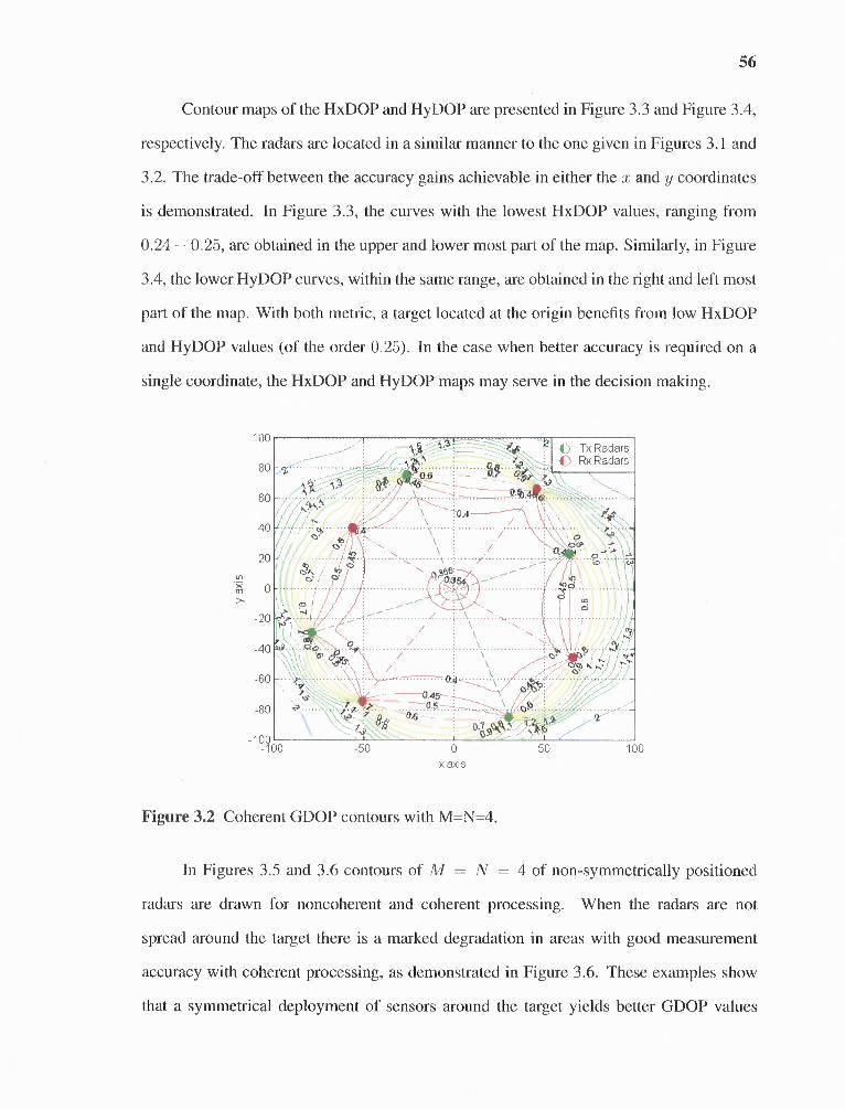
56
Contour maps of the HxDOP and HyDOP are presented in Figure 3.3 and Figure 3.4,
respectively. The radars are located in a similar manner to the one given in Figures 3.1 and
3.2. The trade-off between the accuracy gains achievable in either the x and y coordinates
is demonstrated. In Figure 3.3, the curves with the lowest HxDOP values, ranging from
0.24 — 0.25, are obtained in the upper and lower most part of the map. Similarly, in Figure
3.4, the lower HyDOP curves, within the same range, are obtained in the right and left most
part of the map. With both metric, a target located at the origin benefits from low HxDOP
and HyDOP values (of the order 0.25). In the case when better accuracy is required on a
single coordinate, the HxDOP and HyDOP maps may serve in the decision making.
Figure 3.2 Coherent GDOP contours with M=N=4.
In Figures 3.5 and 3.6 contours of NT = N = 4 of non-symmetrically positioned
radars are drawn for noncoherent and coherent processing. When the radars are not
spread around the target there is a marked degradation in areas with good measurement
accuracy with coherent processing, as demonstrated in Figure 3.6. These examples show
that a symmetrical deployment of sensors around the target yields better GDOP values

Figure 3.3 Coherent HxDOP contours with M=N=4.
57
Figure 3.4 Coherent HyDOP contours with M=N=4.
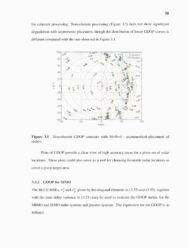
58
for coherent processing. Noncoherent processing (Figure 3.5) does not show significant
degradation with asymmetric placement, though the distribution of lower GDOP curves is
different compared with the one observed in Figure 3.1.
Figure 3.5 Noncoherent GDOP contours with M=N=4 - asymmetrical placement ofradars.
Plots of GDOP provide a clear view of high accuracy areas for a given set of radar
locations. These plots could also serve as a tool for choosing favorable radar locations to
cover a given target area.
3.3.2 GDOP for SIMO
The BLUE MSEs, a,,2 and o, given by the diagonal elements in (3.32) and (3.39), together
with the time delay variance in (3.21) may be used to evaluate the GDOP metric for the
MIMO and SIMO radar systems and passive systems. The expression for the GDOP is as
follows:

59
Figure 3.6 Coherent GDOP contours with M=N=4 - asymmetrical placement of radars.
(3.49)
(3.50)
The GDOP reduces the combined effect of the locations to a single metric. In this
case, the metric is a representation of the square root of the spatial advantage, exemplified
through the trace of matrices 1-1,,,,,„ and I-Isi„,. Once the values are mapped, the actual
localization overall accuracy Vax2 ay2 is easily derived by multiplying the GDOP value
by Ca,.
In Figure 3.7 contour plots of the GDOP values are presented for a coherent MIMO
radar system with M = 3 and N = 5 transmit and receive radars, respectively, positioned
symmetrically on the K = M N = 8 vertices of a polygon centered at the origin. In
Figure 3.8, GDOP plots for a coherent SIMO radar system with one transmitter, M = 1,
and N = 15 receivers are drawn, where the radars are positioned symmetrically on the

60
Figure 3.7 GDOP contour maps for coherent MIMO radar with M = 3 transmitters andN = 5 receivers - case I.
Figure 3.8 GDOP contour maps for coherent SIMO radar with M = 1 transmitter andN = 15 receivers - case I.
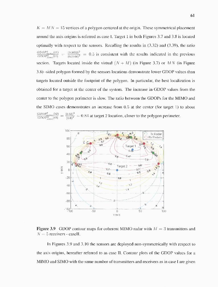
61
K = MN = 15 vertices of a polygon centered at the origin. These symmetrical placement
around the axis origins is referred as case I. Target 1 in both Figures 3.7 and 3.8 is located
optimally with respect to the sensors. Recalling the results in (3.32) and (3.39), the ratioGDOPZ mimo (t1) = (0.3652)²
= 0.5 is consistent with the results indicated in the previousGDOP²simo = (0.5164)²
section. Targets located inside the virtual (N M) (in Figure 3.7) or MN (in Figure
3.8) -sided polygon formed by the sensors locations demonstrate lower GDOP values than
targets located outside the footprint of the polygon. In particular, the best localization is
obtained for a target at the center of the system. The increase in GDOP values from the
center to the polygon perimeter is slow. The ratio between the GDOPs for the MIMO and
the SIMO cases demonstrates an increase from 0.5 at the center (for target 1) to about
GDOP²mimo(t2) = (0.6)² =(0.55)² 0.84 at target 2 location,GDOP²simo(t2) = on, closer to the polygon perimeter.o
I-) Tx Radaro Rx Radars
Figure 3.9 GDOP contour maps for coherent MIMO radar with /14- = 3 transmitters andN = 5 receivers - caseII.
In Figures 3.9 and 3.10 the sensors are deployed non-symmetrically with respect to
the axis origins, hereafter referred to as case II. Contour plots of the GDOP values for a
MIMO and SIMO with the same number of transmitters and receivers as in case I are given

62
Figure 3.10 GDOP contour maps for coherent SIMO radar with M = 1 transmitter andN = 15 receivers - case II.
in these figures. For both, the spatial advantage does not reach the optimal value obtained in
GDOP² (t1) the symmetrical case. For target 1 in Figure 3.9 and 3.10, the ratio ) = 0.466 < GDOP²simo(t1)
0.5, i.e., the SIMO case experience a higher lose in performance compared with the MIMO
scheme. This is further emphasized by target 2, where in the SIMO case GDOP²simo(t2) >
1 while GDOP,72„,„„(t2) 0.5. Case II indicates that for non-symmetrically deployments
of sensors, a larger degradation in the coverage area benefiting from spatial advantage is
observed with SIMO systems vs. MIMO systems.
3.4 Conclusions
Analytical expressions were derived for the MSE of the BLUE estimator for the cases of
coherent MIMO and SIMO radar systems with widely distributed antenna. Both systems
benefit from a spatial advantage imparted by the wide footprint of the multiple sensors. It
turns out that when the sensors are placed optimally with respect to the target, the MIMO
63
configuration with M transmitters and N receiers (i.e., M + N total sensors) has twice the
spatial advantage of SIMO systems with 1 transmitter and MN receivers (i.e., 1 + MN
total sensors). This advantage is inherent in the GDOP metric and is directly related to
the layout of the sensors with respect to the target and the number of transmitting and
receiving radars. The GDOP plots offer a clear insight into the relation between sensor
configuration and localization accuracy. These plots demonstrate the superiority of MIMO
systems over SIMO schemes in both spatial advantage and the resources required to achieve
these performances.
CHAPTER 4
MULTIPLE TARGETS LOCALIZATION
The study of the single target case is extended to the case of multiple targets localization
with coherent MIMO radar systems, dealing with the possible trade-offs that the increased
number of targets impose on the localization accuracy performance. The CRLB is derived
and evaluated for this case. Coherency and spatial advantages are identified and analyzed.
As the spatial advantage is strongly reliant on the geographical setting of the radars with
respect to the targets and on the geometric distribution of targets, an insight into the system
inherent trade-offs is provided using numerical analysis.
4.1 System Model
Assume M transmitting radars and N receiving radars, widely distributed and time and
phase synchronized. The receiving radars could be colocated with the transmitting ones or
widely separated. The transmitting and receiving radars are located in a two dimensional
plane (x, y). Consider Q point targets located at coordinates Xq (xq, yq) , q = 1, Q
(see Figure 4.1). A set of orthogonal waveforms is transmitted, with the lowpass equivalent
sk (t) , k = 1, . . . , M. The power of the transmitted waveforms is normalized such that
the aggregate power transmitted by the sensors is constant, irrespective of the number of
transmit sensors. Let all transmitted waveforms be narrowband signals with individual
effective bandwidth Ok defined as N = (fwk f2ISk(1)12 df) / (fwk1Sk (1)12 df)],
where the integration is over the range of frequencies with non-zero signal content Wk [29].
The signals are narrowband in the sense that for a carrier frequency of fc, the narrowband
signal assumption implies OZ/ fi < 1. Assume the Q targets are located in a search cell
of ±W/2. The target model follows the one developed in [42], generalizing the complex
target model in [29] to a near-field scenario and distributed sensors. In [42] it is shown
64
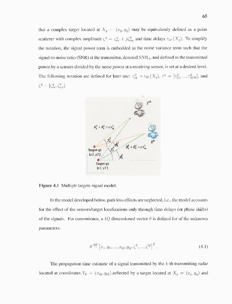
65
that a complex target located at Xq = (xq, yq) may be equivalently defined as a point
scatterer with complex amplitude q = jan and time delays Ta (Xu). To simplify
the notation, the signal power term is embedded in the noise variance term such that the
signal-to-noise ratio (SNR) at the transmitter, denoted SNR t, and defined as the transmitted
power by a sensors divided by the noise power at a receiving sensor, is set at a desired level.
The following notation are defined for later use: TA = Tek (X q), Tq = [41, ...,TckNi, and
q = [qre, rim]
Figure 4.1 Multiplr targets signal model.
In the model developed below, path loss effects are neglected, i.e., the model accounts
for the effect of the sensors/target localizations only through time delays (or phase shifts)
of the signals. For convenience, a 4Q dimensioned vector 0 is defined for of the unknown
parameters:
(4.1)
The propagation time estimate of a signal transmitted by the k-th transmitting radar
located at coordinates Tk (xtk, ytk),reflected by a target located at Xq = (xq, N) and
66
(4.2)
received by a radar located at Re = (xr,e, yre) can be expressed as:
where 1, the propagation time, is the sum of the time delays from radar k to target q and
from the target to radar t:
(4.3)
and EL is the estimation error. The speed of light is denoted by c.
Consider the case of a baseband representation of the signal observed at sensor E due
to a transmission from sensor k and reflection from Q scatterers, given by:
(4.4)
where pqa accounts for the phase information and has the value of 4 = exp (—j27rfcrA).
Others terms are the carrier frequency fc and we (t) is circularly symmetric, zero-mean,
complex Gaussian noise, spatially and temporally white with autocorrelation function
oZS (T). Define the vectors r = [ri (t) , • • • , r N (t)]T and lp = [Ti- . .. , TQ , 0 , .. , (Q]7' for
later use. The received signal at each sensor is a mixture of the transmitted signals reflected
by the targets. The mixture of signals is separated at the receiver end by exploiting the
orthogonality between the transmitted waveforms.
67
4.2 The CRLB on Targets Location Estimation
The CRLB provides a lower bound for the mean square error (MSE) of any unbiased
estimator for an unknown parameter(s). Given a vector parameter 0, its unbiased estimate
satisfies the following inequality [26]:
(4.5)
where J (0) is the Fisher Information matrix (FIM) given by:
(4.6)
where p (1.10) is the joint probability density function (pdf) of 0.
Let the CRLB matrix be defined as:
(4.7)
(4.8)
where J (0) is the FIM for the unknown vector defines as:
J() = Eip {-a
log p (op) (—a
log p (r0)) (4.9)

68
The matrix D represents is of the form:
(4.10)
where the submatrix Dq is derived as:
(4.11)
By using the relation given in (4.3) in (4.11), the Dq matrix is calculated, resulting in:
(4.12)
(4.13)
where the phase oqk is the bearing angle of the transmitting sensor k to target q measured
with respect to the x axis; the phase çal is the bearing angle of the receiving radar i to target
q measured with respect to the x axis. See illustration in Figure 4.1. Matrix Dq includes
the geometric information of the radars location configuration relative to the position of theqt h target.
In order to derive the FTM given in (4.9) the joint pdf p (rill)) is required. Given
a set of known waveforms sk (t — 1) parameterized by the unknown time delays 'a,
which in turn are a function of the unknown targets locations Xq = (xq, yq), for the signal
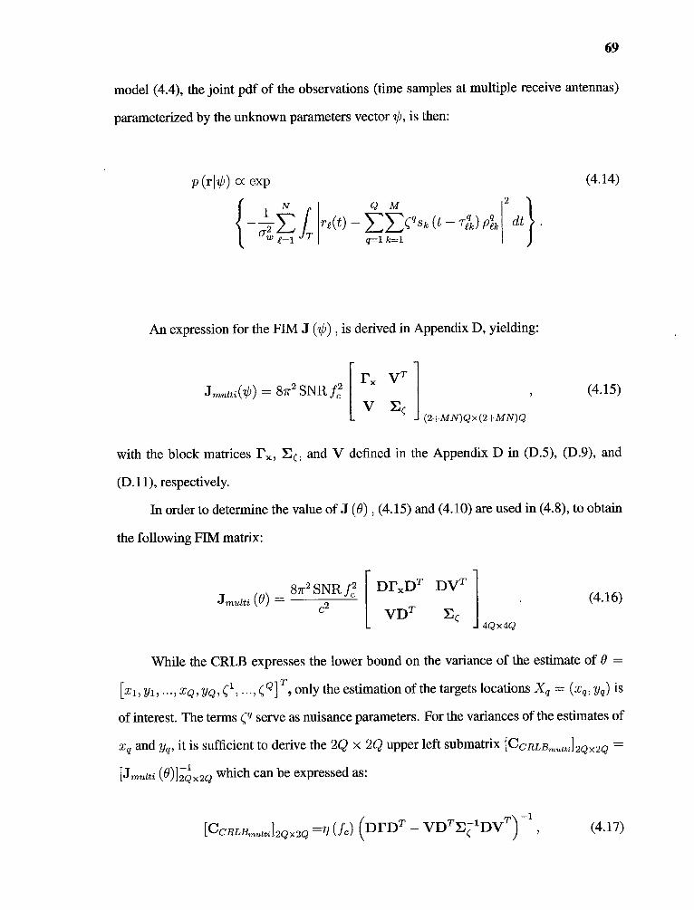
69
model (4.4), the joint pdf of the observations (time samples at multiple receive antennas)
parameterized by the unknown parameters vector 0, is then:
(4.14)
An expression for the FIM J (0) , is derived in Appendix D, yielding:
(4.15)
with the block matrices Tx, Ec, and V defined in the Appendix D in (D.5), (D.9), and
(D.11), respectively.
In order to determine the value of J (0) , (4.15) and (4.10) are used in (4.8), to obtain
the following FINI matrix:
(4.16)
While the CRLB expresses the lower bound on the variance of the estimate of 0 =
xQ, YQ, • ••,
1 T, only the estimation of the targets locations Xq = (xq, yq) is
of interest. The terms q serve as nuisance parameters. For the variances of the estimates of
xq and yq, it is sufficient to derive the 2Q x 2Q upper left submatrix [CCRLBm ulti] 1 2Q x 2Q =
Antati (0)} 2—Q1 x 2Q which can be expressed as:
(4.17)

70
e2 where n (fc) = 87r² SNR f²c• The diagonal elements of the submatrix [CCRLBmulti]ulti] 2Q x 2Q
provide the lower bound on the localization mean squared error (MSE), ax2, aCRx, =
(4.18)
(4.19)
(4.20)
The CRLB matrix is related to the sensors and targets locations through matrices D,
Fx and V, while the latter two are also functions of the received waveforms correlation
functions and its derivatives. This dependency is captured in the terms 71S* (Xg ) and
nspt (yq), where further analysis is required.
4.3 Discussion
The expression for the CRLB as given in (2.38), provides insight into the performance of
multiple targets localization accuracy performance of MIMO radars systems with coherent
processing.
Coherency advantage As in the single target case, the lower bound on the targets
localization errors is inversely proportional to the carrier frequency L and independent of
the signal individual effective bandwidth, due to the use of the phase information across the
different paths. It is apparent that coherent processing offers a target localization precision
gain of the order of MO, referred to as coherency advantage.

71
The improvement in localization accuracy needs to be moderated with the
observation that the CRLB is a bound of small errors. As such, it ignores effects that
could lead to large errors. For example, MIMO radar with distributed sensors and coherent
observations is subject to high sidelobes [1]. Additionally, a phase coherent system is
sensitive to phase errors. These topics are outside the scope of this paper, but they should
be kept in perspective.
Spatial advantage The CRLB submatrix terms are strongly reliant on the relative
geographical spread of the radar sensors versus the targets locations. In MIMO radar, the
targets play a similar role to the transmission channel in NLIMO communication. As such,
the elements in the CRLB, re and Vqq', q qt may be viewed as overlapping multipath
arrivals for a given tk propagation path. The trace of the CRLB provides an averaged
(4.21)
where *gig = EZ-1. The first two terms in (4.21) are the auto-correlation terms, while the
third term represents the cross-correlation between targets and therefore, serves as mutual
interference. The elements of these cross-correlation matrices are products of the phase and
amplitude elements, exp (-27LATZ') and f sk (t — ZNale) 4 (t) dt, where AT -=
—7-4, and its derivatives (see (D.5) and (D.11) in Appendix D). As the distance between
the targets impacts the time delay differences, ATIZ', the following might be gleaned by
inspection of (4.21):
• Targets separated by distances larger than a c/f3 resolution cell are resolvable with
negligible loss in performance relative to the single target case. This results from the
decorrelation achieved by this scenario, where the third term in (4.21) approaches

72
zero. On the other end, distances smaller than the carrier wavelength A are non-
resolvable.
• The interference on paths a for target q add in-phase with c τqq'lku, u = 0,1,2, ...,
i.e. cos (-2r fc τqq'lk) 1. They add out-of-phase with etk u, u = 1,2, ..., i.e.
cos (-27rfcATZ0 < 1. It is evident that the number of resolvable paths varies with
the position of the radars with respect to the targets and the targets layout, where
some may be more favorable than others. The number of resolvable propagation
paths per target q and the geometric merit of these paths (integrated in matrix Dq)
determines the ability to localize target q and the localization accuracy quality. A
minimum of 3 resolvable paths is required for the localization of a single target.
• Transmit and receive radar pairs, a, with large aperture with respect to the targets
layout are preferable due to the larger time delay differences they offer.
• Sensors placement needs to take into account the vertical and horizontal plane
sensitivity needed for a given targets layout. For example, a horizontal targets
layout requires better horizontal separation, achieved by broadside horizontal radar
geometry.
To get a more intuitive understanding of the reliance of the spatial advantage on the
geographical spread of the radars and targets, numerical analysis is employed in the next
section for some special cases.
4.4 Numerical Analysis
The spatial advantage in the case of a single target is derived in [42]. It is shown to be
equals 2/MN under optimal conditions, i.e. when the target is located at the center of a
virtual circle created by the radars, and the radars are spread with equal angular spacing
with respect to the center (2π/M (2π/M and 2π/N) or any superposition of such symetrical placments.
The value of the spatial advantage for any possiable target location with a given radar layout

73
was evaluated using a metric known as geometric dilution of precision (GDOP). In the case
of multiple targets, the spatial advantage relies on the the number of targets and their layout
in addition to the radar locations. For this reason, numerical analysis of the expresion in
(4.20) for some special cases is employed in this section.
The value of the spatial advantage TiSpatial is anaylazed for various radars/targets
placements senarios. System parameters are set as follows: = /3 = 200KHz, carrier
frequency fc = 2GHz and therefore, the wavelength is A = 1.5meter, SNR=20 and
all reflectivity index values are assumed equal 101 = = 1. In Figure (4.2) the
spatial advantage value is drawn for the case of M = 3 transmit antennas employed
with N = 3, 4, 5 receive antennas. Both transmit and receive antennas are located with
angular spacing of 1/1-1. and with respect the the axis origin. Targets are located in a linear
array with the first target located at (0,0) and the rest located at (xq = xq_i + 10, yq = 0).
At Q = 1, the resulting spatial advantage in Figure (4.2) follow the results for a single
target where the values of t , , and are obtained. It is observed that an increas in
the number of targets results in a decrease in the spatial advantage and therefore, in the
accuracy. This decreas may be moderated by increasing the number of transmit and receive
radars, MN. In the case of M = N = 3 three targets enjoy spatial advantage while with
M = 3 and N = 5 six targets still benefit from spatial advantage. For the later case,
up to four targets are located with high accuracy. In Figure (4.3) the spatial advantage of
the x and y axis is draw separtly for the same senario as in Figure (4.2). It conveys the
way in which each of the axis performs. It demonstrates that the axis accurecies might
vary significantly for the x and y axis. Moreover, the performance gap shrinks as the
number of transmit and reveice radar increases, due to the aditional, spatially spread, view
points. As mentioned previously, the spatial advantage for the case of a single target is
MN/ 2 under optimal conditions, i.e. when the target is located at the center of a virtual
circle created by uniformly spaced sensors. In the case of multiple targets, the spatial
advantage relies on the number of targets and their layout relative to the sensors locations.
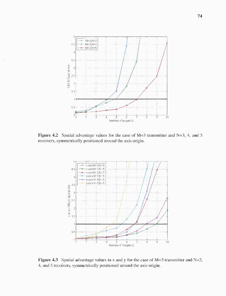
74
Number of targets Q
Figure 4.2 Spatial advantage values for the case of M=3 transmitter and N=3, 4, and 5receivers, symmetrically positioned around the axis origin.
Figure 4.3 Spatial advantage values in x and y for the case of M=3 transmitter and N=3,4, and 5 receivers, symmetrically positioned around the axis origin.

75
Figure 4.4 System layout for cases 1 to 4.
To identify favorable radars locations with respect to the targets layout, four special cases,
demonstrated in Figure (4.4), are analyzed.
The averaged value of Tispt versus the number of targets is drawn in Figure (4.5).
Following the discussion in previous section, one needs to avoid Arl:' 0 and keep ATZ'
as large as possible. It is observed in the figure that a symmetrical placement, as shown in
Case 1, is not an optimal one. Rearranging the radars, in the more favorable setting (as in
Case 4) demonstrates a performance gain, in terms of the number of targets and the spatial
advantage, achieved without any change in the number of antennas. This is a result of the
larger transmit/receive aperture sets contributing to larger delays. Placing the radars in a
broadside horizontal spread (as in Case 3) provides better spatial advantage and moderate
performance loss rate when compared with Case 2, where a vertical radar setting is used.
This is a combined effect of the larger time delays and the impact of matrix D, which
provide better horizontal separation in Case 3 [68]. Increasing the number of radars, as can
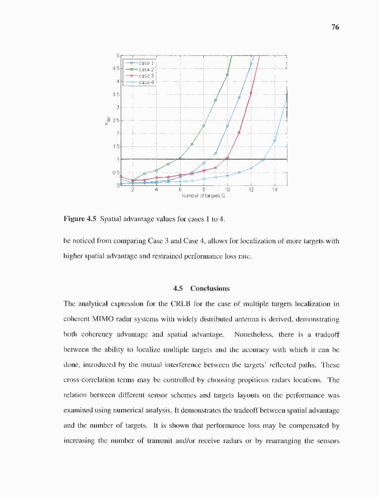
76
Figure 4.5 Spatial advantage values for cases 1 to 4.
be noticed from comparing Case 3 and Case 4, allows for localization of more targets with
higher spatial advantage and restrained performance loss rate.
4.5 Conclusions
The analytical expression for the CRLB for the case of multiple targets localization in
coherent MIMO radar systems with widely distributed antenna is derived, demonstrating
both coherency advantage and spatial advantage. Nonetheless, there is a tradeoff
between the ability to localize multiple targets and the accuracy with which it can be
done, introduced by the mutual interference between the targets' reflected paths. These
cross-correlation terms may be controlled by choosing propitious radars locations. The
relation between different sensor schemes and targets layouts on the performance was
examined using numerical analysis. It demonstrates the tradeoff between spatial advantage
and the number of targets. It is shown that performance loss may be compensated by
increasing the number of transmit and/or receive radars or by rearranging the sensors
77
locations. As the CRLB provides a good bound at high SNR, a more rigid bound needs
to be found for the low SNR case, where the ambiguities predominate the estimation
capabilities.

CHAPTER 5
SENSITIVITY ANALYSIS TO PHASE SYNCHRONIZATION MISMATCH
Improvement in target parameter estimation capabilities is among the advantage of MIMO
radar systems [1, 42]. In particular, target localization with coherent MIMO radar
systems, utilizing widely distributed antennas, offers significant advantages [42]. Typically,
performance analysis of system parameter estimation problems is based on the derivation
of the Cramer-Rao bound (CRB), which sets a lower bound on the estimation MSE for
unbiased estimators. Such an evaluation is provided in Chapter 2 for coherent MIMO radar
systems, demonstrating a localization accuracy advantage, inversely proportional to the
signal carrier frequency. In addition, a spatial advantage of the order of the product of the
number of transmit and receive radars is also incorporated in the CRB.
This performance gain comes with the challenge of attaining phase synchronization
in a distributed system. Errors introduced to the system parameters by phase
synchronization mismatch, will result in parameter estimation mean-square error (MSE)
degradation and bias. In this work, the hybrid CRB (HCRB) is used to test the sensitivity
of the target localization MSE to phase errors. The HCRB takes into account deterministic
unknown parameters, such as the target location, as well as random parameters, phase
calibration errors, in this case. This method has been applied to passive source localization
[69], [70] for the problem of source bearing and range estimation with uncertainty in the
sensors' locations or phase synchronization errors.
In this chapter, the HCRB is derived for coherent Mitv10 radars, with phase
synchronization errors. A closed-form expression for the HCRB for the target's location
(x, y) is derived, providing the means to assess the effects of phase errors on the localization
accuracy. The effect of the number of radars, their geometric layout, and the phase
mismatch MSE is incorporated in the HCRB terms.
78
79
In this study, the hybrid Cramer-Rao bound (CRB) is developed for target
localization, to establish the sensitivity of the estimation mean-square error (MSE) to
the level of phase synchronization mismatch in coherent Multiple-Input Multiple-Output
(MIMO) radar systems with widely distributed antennas. The lower bound on the MSE
is derived for the joint estimation of the vector of unknown parameters, consisting of the
target location and the mismatch of the allegedly known system parameters, i.e., phase
offsets at the radars. Synchronization errors are modeled as being random and Gaussian.
A closed-form expression for the hybrid CRB is derived for the case of orthogonal
waveforms. The bound on the target localization MSE is expressed as the sum of two
terms - the first represents the CRB with no phase mismatch, and the second captures
the mismatch effect. The latter is shown to depend on the phase error variance, the
number of mismatched transmitting and receiving sensors and the system's geometry. For
a given phase synchronization error variance, this expression offers the means to analyze
the achievable localization accuracy. Alternatively, for a predetermined localization
MSE target value, the derived expression may be used to determine the necessary phase
synchronization level in the distributed system.
5.1 Background
The hybrid CRB provides a low bound on the MSE of any unbiased estimator for an
unknown parameter(s), where the parameters are partially deterministic and partially
random [28]. Given a vector parameter 0 = [0„,, OriT , where On, stands for the nonrandom
parameter vector and Or for a random parameter vector, its unbiased estimate -6" satisfies the
following inequality [28]:
(5.1)
where JH (0) is the hybrid Fisher Information matrix (HFIM) expressed as
(5.2)

80
The elements of the matrices JD and Jp given by
(5.3)
where p(r|θnr, θr) is the conditional, joint probability density function (pdf) of the
observations and p (θr |θ nr) the conditional joint pdf of θ. The matrix JD represents the
contribution of the data and the matrix Jp represents the contribution of prior information.
The HCRB matrix is defined as
(5.4)
In cases in which the observation statistic is expressed in terms of p (rlicnr, Kr), and
the relationship between the unknown parameters Onr, Or and krir, Kr is given by ni =
the chain rule, can be used to express J H (Onr, Or) in an alternative form [261:
(5.5)
where the elements of the matrix P are given by [Ph 4 =
5.2 HCRB with Phase Mismatch
In this section, the HCRB is developed for target localization. A point target is assumed
with complex reflectivity t9 = Re + ± jϑIm, located in a two dimensional plane at coordinates
X = (x, y). Consider a set of M transmitting stations and N receiving stations, widely
distributed over a given geographical area, and time and phase synchronized. A set of
orthogonal waveforms is transmitted, with the lowpass equivalents sk (t) , k = 1,... ,M,
and effective bandwidths )3 [29]. The signals are narrowband in the sense that for a carrier
frequency of fe, the narrowband signal assumption implies )3²c/ f²c << 1
81
In [42], perfect phase synchronization was assumed. In practice, synchronization
errors exists, modeled here as zero mean Gaussian random variables with standard
deviation al and denoted by AO = 1 Jot A42, .•., AOtivn AOri) AOT2 " • , AOr/sT1T, where
A0t, and 6.0r, are phase errors at transmitting radar k and receiving radar t, respectively.
The phase errors introduced by the different stations are assumed to be statistically
independent. The vector of unknown parameters is defined by
(5.6)
where Onr [x, y, Vize, Vim] denotes the deterministic unknowns and Or -= AOT denotes
the random unknowns.
The estimation process is based on the signals observed at the receiving sensors. The
signal received at sensor t is a superposition of the transmitted signals, reflected from the
target, and given by:
(5.7)
where nEk accounts for the phase information and has the value of nek =
exp (— j271 LrEk) exp (—j (AOt, + .6. The noise nE (t) is assumed to be circularly
symmetric, zero-mean, complex Gaussian, spatially and temporally white with
autocorrelation function cr,i26 (T). The propagation time, rtk, is a sum of the time delays
from station k to the target and from the target to station t, and may be expressed as
(5.8)
where c denotes the speed of light, (xtk, ytk) denotes the location of transmitting radar k
and (x,E,YrE) denotes the location of receiving radar f. The following vector notation is
introduced: T [T11) T12) Ttk) • --) TArM] T.

82
The received signals are separated at the receiver by exploiting the orthogonality
between the transmitted waveforms. The signal in (5.7) is defined as a function of the
time of arrival, Tek, the reflectivity value 19, and the phase mismatch AO. The vector of
unknown parameters for the observations re (t) is expressed as a function of the time delays
'T rather than a function of the unknown location (x, y) (as seen in (5.8)); i.e., the vector
of unknown parameters is denoted by lc = krir, kr , with = [IT Ike 'Olin] and kr =
AOT. The following notation is defined for later use: r = [ri (t) , , r N (t)], Q = MN,
L = M + N.
In order to derive the HFIM given in (5.2) and (5.3), the conditional joint pdf p (r1k)
is required. For the signal model given in (5.7), the conditional joint pdf of the observations
(time samples at multiple receive antennas) parametrized by the unknown parameters
vector IC, is then
(5.9)
The observation is given as a function of k. Therefore, the matrix P, defined following
(5.5), needs to be derived. The relation given in (5.8) is used, resulting in
(5.10)
(5.11)
with
83
where cxk is the bearing angle of the transmitting sensor k to the target, measured with
respect to the x axis, and 'ye is the bearing angle of the receiving radar t to the target,
measured with respect to the x axis.
Using the conditional pdf p (r 1 /0 in (5.9) and the Gaussian distribution of the phase
errors, the HFIN4 J H (10 , defined by (5.2) and (5.3), is derived in Appendix E, resulting in
(5.12)
(5.13)
(5.14)
and the other submatrices in (5.12), (5.13) and (5.14) are defined and derived in Appendix
E (see (E.1), (E.3), (E.4) and (E.5)). Applying (5.10) and (5.12) in (5.5) yields
(5.15)
The HCRB for the unknown parameters (x, y) may be derived from (5.15), applying the
relation given in (5.4) :
HCRB (x, y) = [DRAY — DGH-¹GTDT]-¹2×2 . (5.16)
84
To find the closed-form solution to HCRB (x, y), the matrix 11--¹ is expressed using the
formula for the inverse of a partitioned matrix [71]:
(5.17)
(5.18)
and
(5.19)
where Ap = (Ep + 1/σ2I). The term [ — F-¹ϑ -¹AA-¹FTϑ] -¹ in (5.17), is transformedσ²
based on the formula for the inverse of a matrix B of the form B = A + XRY, given
in [71]. Following some additional matrix manipulations, the HCRB for the location MSE
can be expressed as
(5.20)
where CRI3, (x, y) = JF-1- is the CRB with no phase mismatch, and
CRB = PFPA--¹JF — JF] represents the increment in the bound due to phase
synchronization errors. The matrices JF and Pp are defined by
(5.21)
85
and the matrix Ra-1 can be calculated recursively using the formula for the inverse of the
sum of matrices [72], resulting in
(5.22)
where 1 = „ 11T and the terms Ai and A²c are
(5.23)
Calculating the explicit value of ACRB, one gets
(5.24)
where the constants km, m = 1, 2, 3 are functions of the phase synchronization error
variance cri (through Ai and A²c, defined in (5.23)) and the number of transmitting and
receiving radars M and N, as follows:
(5.25)
The matrices Bni, m = 1, 2, 3 depend on the geographical layout of the radars with respect
to the target location:
86
using the following Dm matrices:
(5.26)
and
The expression for the HCRB as given in (5.20), offers an interesting observation on the
effects of phase errors on the target localization MSE. First, it is apparent that the HCRB
may be expressed as the sum of the CRB with no phase error and a term dependent on the
statistics of the phase errors. This term is a function of the sensors location with respect
to the target, through the matrices Bm, and the system parameters (SNR, phase errors
variance cri and the number of mismatched transmitting and receiving radars) through
the coefficients pm. The manner in which the number of radars, their spread and the phase
synchronization error variance affect the performance is not readily understood from (5.24).
For this reason, numerical examples are employed in the next section to gain some insight
into the relationships between system parameters and performance degradation.
5.3 Numerical Analysis
The HCRB expression given in (5.20) is numerically evaluated using the following
example: M = 11, N = 9 and cri = [0, 0.0001, 0.0005, 0.001, 0.005, 0.01, 0.051, where
al is expressed in (rad²c). The HCRB (x,, yo) is drawn in Figure 5.11. As a2a increases
beyond a specific value, the additional CRB term ACRB dominates the performance and
the curve. For high phase error levels, the performance degradation starts at lower SNRs.

87
Figure 5.1 HCRB for M=11 and N=9. The blue line represent the CRB value with nophase errors.
For small phase errors, localization accuracy is not undermined by the phase mismatch,
and the HCRB (xo, ye) curve follows the CRI30 (xo, ye) closely.
For a given system, the tolerated [ail. may be determined by solving
ACRB ([σ²]max) CRBo (xo, ye). This value can serve as a design goal in the system
phase calibration. For a given phase synchronization error variance (72A, the expression
ACRB (o-i) gives the localization accuracy penalty.
5.4 Conclusions
MIMO radar with coherent processing exploits the signal phase measured at the receive
antennas to generate high resolution target location estimation. To take advantage of this
scheme, full phase synchronization is required among all participating radars. In practice,
inevitable phase synchronization errors reflect on the system localization performance.
In this paper, a closed-form expression of the HCRB of target localization has been
88
derived, capturing the impact of the phase synchronization errors on the achievable target
localization accuracy. In particularly it has been shown that the HCRB can be expressed
as a sum of the CRB with no phase error and a term that represents the phase error
penalty. The latter has been shown to be a function of the sensors geometry, SNR, and
the number of transmitting and receiving radars in addition to the phase error MSE. As
phase synchronization over distributed platform is a complex operation and phase errors
are unavoidable, the HCRB offers valuable information at the system design level. For a
given phase error MSE, the HCRB may be used to derive the attainable target localization
accuracy. Otherwise, for a given system performance goal on localization accuracy, the
HCRB provides with an upper bound on the necessary phase error MSE values.
CHAPTER 6
TARGET TRACKING IN MIMO RADAR SYSTEMS
Target tracking as it is an essential requirement for surveillance systems [73-751 Herein,
target tracking performances of MIMO radar systems are evaluated. The joint Bayesian
Cramer-Rao bound (BCRB) [28] is formulated, and a recursive bound on the state
variables (target location and velocity) is derived based on the nonlinear filtering bound
developed in [76]. A BCRB based analysis for multi-static radar systems is provided
in [77]. The system model assumes one transmitter and multiple receivers. Target position
estimation performance is demonstrated for a given target path, yet limited insight is
provided as to the dependency of this bound on system parameters. In this study, the
effect of system parameters on target tracking performance is presented. Based on this
study, two tracking schemes are proposed. The first is a centralized architecture, based
on joint processing of either raw or partially processed (compressed) data at a fusion
center. This approach provides highly accurate target tracking and takes full advantage
of the MIMO configuration. The second is a decentralized scheme, based on a hybrid
combination of local processing at the receiving radars and joint tracking at a fusion center.
The latter approach supports resource aware system operation. Reduced communication
requirements and processing load may be achieved with relatively low performance cost
with the proposed decentralized method.
In this Chapter, the study of target localization in MIMO radar systems with
distributed antennas and noncoherent processing is extended to target tracking. The BCRB
on target location and velocity is derived, and insight is gained into the effect of the
radars geometric layout and the target location on tracking accuracy. The relation between
estimation error and the number of radars is examined and the contribution of target
reflectivity and path loss to tracking performance is evaluated. Adaptive tracking tactics are
89

90
proposed, accounting for the target parameters estimation accuracy and the radar sensors
spread.
6.1 System Model
Assume M transmitting radars and N receiving radars, widely distributed, and time
and phase synchronized. The receiving radars could be collocated with the transmitting
elements or widely separated. The transmitting and receiving radars are located in a
two dimensional plane (x, y). Consider a single moving complex target with an initial
location (x0, yo) and velocity (i, , . At state n, defines as the time interval ndt, where
At is the observation interval, the target is located at coordinates (xn, yn) (see Figure
6.1). A set of orthogonal waveforms is transmitted, with the lowpass equivalent sk (t) ,
k = 1, . . . , M. The power of the transmitted waveforms is normalized such that the
aggregate power transmitted by the sensors is constant, irrespective of the number of
transmit sensors. Let all transmitted waveforms be narrowband signals with individual
effective bandwidth fik defined as 131! = [(fw, f²c isk (1)1²c df) / (fwkISI (1)1²c df)], and
an effective time duration Tbk defined as nk =[( t² |[(ʃTk -2 |Sk (t)1²c dt) (LI 1Sk (t)1²c dt)] ,
where the integration is over the range of frequencies with non-zero signal content Wk [29].
The signals are narrowband in the sense that for a carrier frequency fc, the narrowband
signal assumption implies ,q/ 1 and S²c/ fi < 1, where /3 = 1+, ESk.k=-¹
The propagation time estimate of a signal transmitted by the k-th transmitting radar
located at coordinates Tk = (Xtk, Ytk), reflected by a target located at (Xn, yn), and received
by a radar located at R,e = (fcr.e, yrt) can be approximated as:
where Tekr, the propagation time, is the sum of the time delays from radar k to the target
and from the target to radar t in state n:
91
(6.2)
and ETekr, is the time delay estimation error. The speed of light is denoted by C.
The Doppler shift estimate of a signal transmitted on the lk-th path can be
approximated as:
(6.3)
where wan, the Doppler shift on the lk-th path due to the target velocity in state n
and ec,) is the Doppler shift estimation error. The term ±, stands for the target velocity
in direction x and Yn, for the target velocity in direction y at the nth state. The phase Okn is
the bearing angle of the target to transmitting sensor k with respect to the x axis; the phase
yoir, is the bearing angle of the target receiving radar t measures with respect to the x axis.
See illustration in Figure 6.1.
Consider the case of a baseband representation of the signal observed at sensor t due
to a transmission from sensor k and reflection from the scatterer at coordinates (xn, yn),
given by:
(6.5)
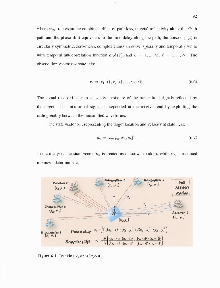
where aekr, represent the combined effect of path loss, targets' reflectivity along the lk-th
path and the phase shift equivalent to the time delay along the path, the noise wf,,, (t) is
circularly symmetric, zero-mean, complex Gaussian noise, spatially and temporally white
with temporal autocorrelation function cr,²c6 (r), and k = 1, ..., M, = 1, , N. The
observation vector r at state n is:
(6.6)
The signal received at each sensor is a mixture of the transmitted signals reflected by
the target. The mixture of signals is separated at the receiver end by exploiting the
orthogonality between the transmitted waveforms.
The state vector xn, representing the target location and velocity at state n, is:
(6.7)
In the analysis, the state vector xn treated as unknown random, while an is assumed
unknown deterministic.
Figure 6.1 Tracking system layout.
93
The state model is a linear motion model, represented as ( [78], [73]):
(6.8)
where vn is modeled as white Gaussian process noise with covariance matrix Qv of the
form:
(6.9)
On:
(6.10)
where d stands for the observation, that in the MIMO radar case is the set of signals
observed at the receiving radars, expressed by 6.5 as a nonlinear function of a vector of
unknown narameters 7h_ defined as:
(6.11)
94
where L = MN.
6.2 The Bayesian Cramer-Rao Bound (BCRB)
In [76], a recursive, multiple dimensional, generalized Bayesian Cramer-Rao Bound
(BCRB) is developed. In general, the BCRB for an unknown vector parameter 0 ERn×¹,
estimated using an observation vector r, is of the form:
(6.12)
where JB is the Bayesian information matrix (BIM), and CB is the BCRB matrix. The
BIM is calculated using the joint probability density function (pdf), as follows:
(6.13)
Based on the relation pr,o (r, 0) = No (r 10) - po (0), it is shown in [76] that the BIM
may be expressed as a linear combination of two matrices:
(6.14)
where JD is the Fisher information matrix (FIM) and represents the information coming
from the data and Jp represents the a priori information, named hereafter as PIM. The FIM
and PIM are derived using:
(6.15)
(6.16)
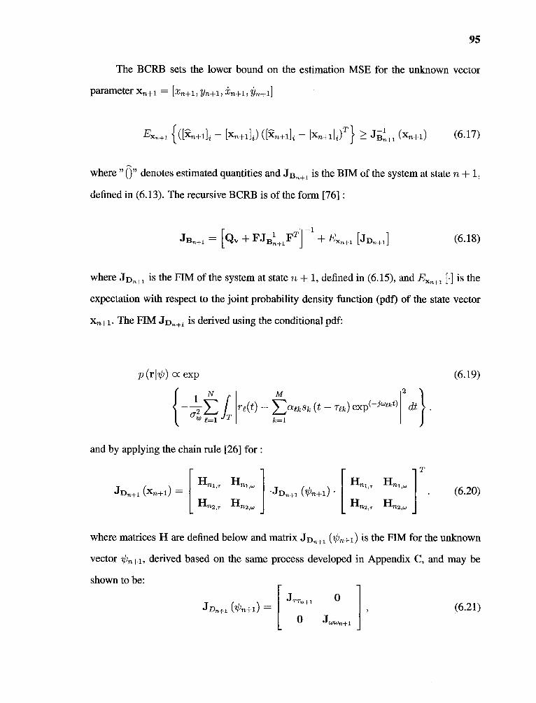
95
The BCRB sets the lower bound on the estimation MSE for the unknown vector
(6.17)
where "0" denotes estimated quantities and J13 is the BIM of the system at state n I,
defined in (6.13). The recursive BCRB is of the form [76] :
(6.18)
where JE,,, is the FIM of the system at state n I, defined in (6.15), and Exn+,[.] is the
expectation with respect to the joint probability density function (pdf) of the state vector
Xn-Fl• The FIM JD„_,1 is derived using the conditional pdf:
(6.19)
and by applying the chain rule [26] for :
(6.20)
where matrices H are defined below and matrix Jr:In+1 (ψn+1) is the FIM for the unknown
vector zi)n-E.-¹, derived based on the same process developed in Appendix C, and may be
shown to be:
(6.21)

96
where matrix J„ is
(6.22)
and matrix J,,_, follows,
(6.23)
Elements of matrices H are provided by the derivative of the expressions in (6.2) and (6.4)
with respect to the state vector in (6.7). It can be shown that:
(6.24)
Using (6.24) and (6.21) in (6.20), yields:
j(6.25)
The lower bound on the state vector estimation error in state n 1, is provided by
the expression in (6.18), integrating the FIM derived in (6.25). Next, numerical analysis
of the BCRB, integrating (6.25) in (6.18) is provided, establishing an understanding of the
tracking performance of MIMO radar systems.
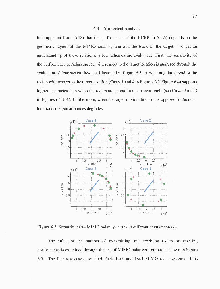
97
6.3 Numerical Analysis
It is apparent from (6.18) that the performance of the BCRB in (6.25) depends on the
geometric layout of the MIMO radar system and the track of the target. To get an
understanding of these relations, a few schemes are evaluated. First, the sensitivity of
the performance to radars spread with respect to the target location is analyzed through the
evaluation of four system layouts, illustrated in Figure 6.2. A wide angular spread of the
radars with respect to the target position (Cases 1 and 4 in Figures 6.2-Figure 6.4) supports
higher accuracies than when the radars are spread in a narrower angle (see Cases 2 and 3
in Figures 6.2-6.4). Furthermore, when the target motion direction is opposed to the radar
locations, the performances degrades.
Figure 6.2 Scenario I: 6x4 MIMO radar system with different angular spreads.
The effect of the number of transmitting and receiving radars on tracking
performance is examined through the use of MIMO radar configurations shown in Figure
6.5. The four test cases are: 3x4, 6x4, 12x4 and 18x4 MIMO radar systems. It is
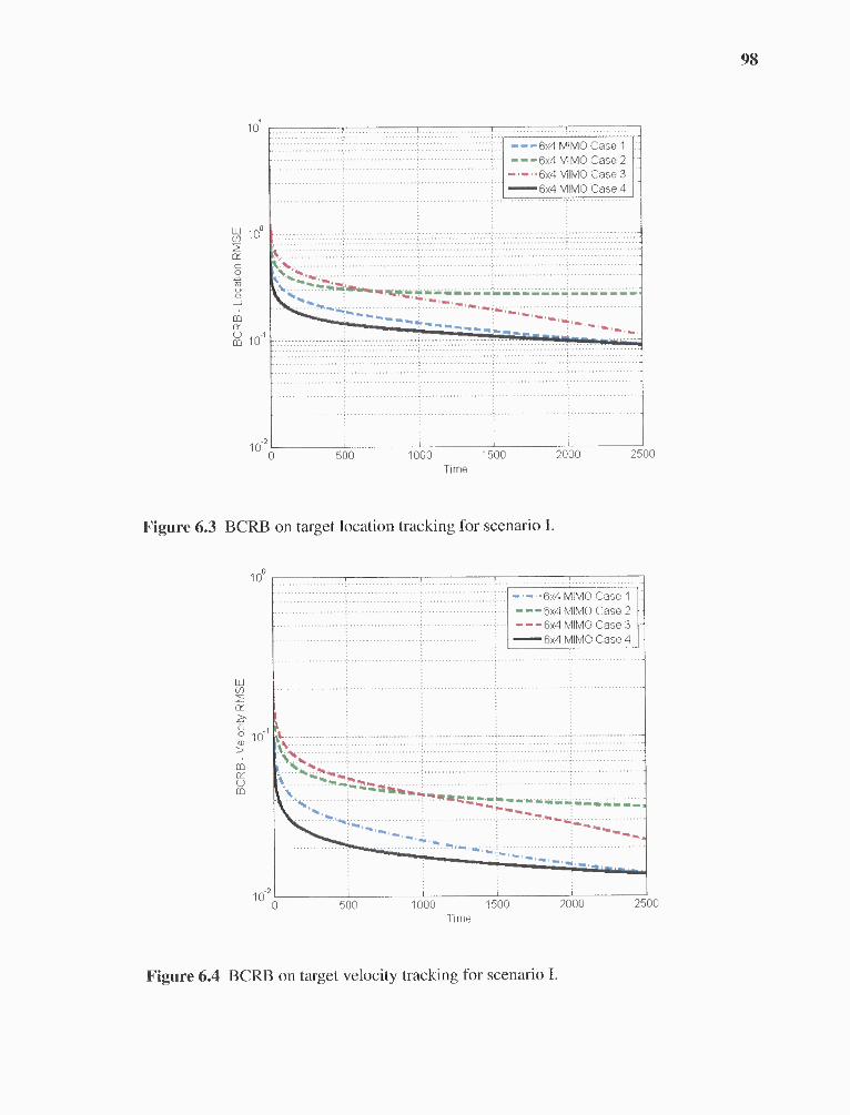
Figure 6.3 BCRB on target location tracking for scenario I.
6x4 MIMO Case 16x4 MIMO Case 26x4 MIMO Case 36x4 MIMO Case 4
98
Figure 6.4 BCRB on target velocity tracking for scenario I.
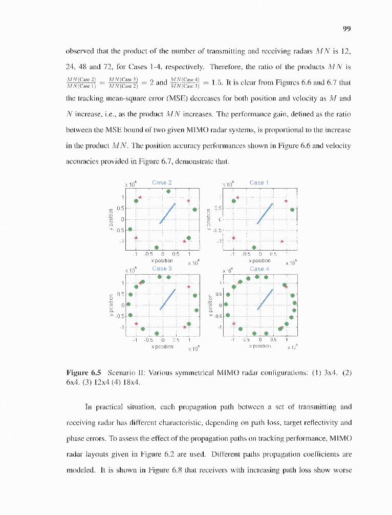
99
observed that the product of the number of transmitting and receiving radars MN is 12,
24, 48 and 72, for Cases 1-4, respectively. Therefore, the ratio of the products MN isMN(Case 2) = MN(Case 3) = 2 and 1.5. It is clear from Figures 6.6 and 6.7 thatMN(Case 4) M N(Case 1) M N (Case 2) MN(Case 3)
the tracking mean-square error (MSE) decreases for both position and velocity as iV/ and
N increase, i.e., as the product MN increases. The performance gain, defined as the ratio
between the MSE bound of two given MIMO radar systems, is proportional to the increase
in the product MN. The position accuracy performances shown in Figure 6.6 and velocity
accuracies provided in Figure 6.7, demonstrate that.
Figure 6.5 Scenario II: Various symmetrical MIMO radar configurations: (1) 3x4. (2)6x4. (3) 12x4 (4) 18x4.
In practical situation, each propagation path between a set of transmitting and
receiving radar has different characteristic, depending on path loss, target reflectivity and
phase errors. To assess the effect of the propagation paths on tracking performance, MIMO
radar layouts given in Figure 6.2 are used. Different paths propagation coefficients are
modeled. It is shown in Figure 6.8 that receivers with increasing path loss show worse
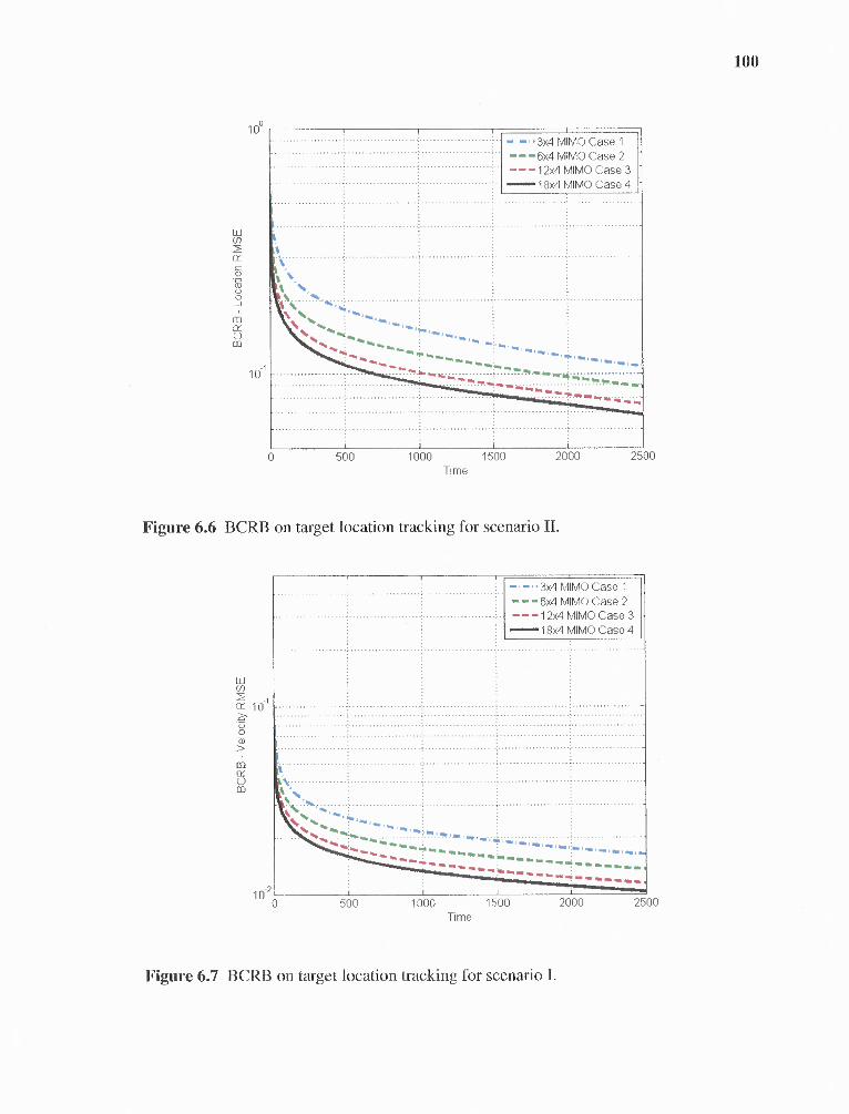
— -3x4 MIMO Case 1—--6x4 MIMO Case 2— — — 12x4 MIMO Case 3
18x4 MIMO Case 4
0 500 1000 1500 2000 2500Ti me
Figure 6.6 BCRB on target location tracking for scenario II.
- — • 3x4 MIMO Case 1• —6x4 MIMO Case 2— — — 12x4 MIMO Case 3
MIMO Case 4
100
Figure 6.7 BCRB on target location tracking for scenario I.
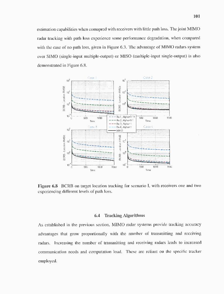
101
estimation capabilities when comapred with receivers with little path loss. The joint MIMO
radar tracking with path loss experience some performance degradation, when compared
with the case of no path loss, given in Figure 6.3. The advantage of MIMO radars system
over SIMO (single-input multiple-output) or MISO (multiple-input single-output) is also
demonstrated in Figure 6.8.
Figure 6.8 BCRB on target location tracking for scenario I, with receivers one and twoexperiencing different levels of path loss.
6.4 Tracking Algorithms
As established in the previous section, MIMO radar systems provide tracking accuracy
advantages that grow proportionally with the number of transmitting and receiving
radars. Increasing the number of transmitting and receiving radars leads to increased
communication needs and computation load. These are reliant on the specific tracker
employed.
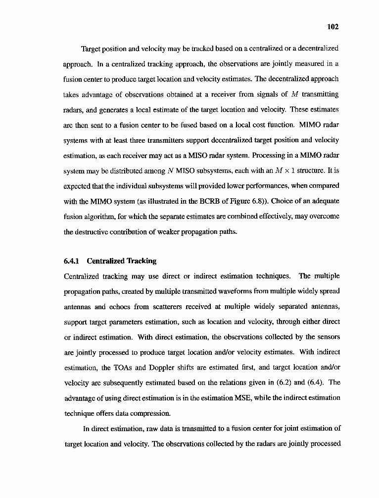
102
Target position and velocity may be tracked based on a centralized or a decentralized
approach. In a centralized tracking approach, the observations are jointly measured in a
fusion center to produce target location and velocity estimates. The decentralized approach
takes advantage of observations obtained at a receiver from signals of M transmitting
radars, and generates a local estimate of the target location and velocity. These estimates
are then sent to a fusion center to be fused based on a local cost function. MIMO radar
systems with at least three transmitters support decentralized target position and velocity
estimation, as each receiver may act as a MISO radar system. Processing in a MIMO radar
system may be distributed among N MISO subsystems, each with an M x 1 structure. It is
expected that the individual subsystems will provided lower performances, when compared
with the MIMO system (as illustrated in the BCRB of Figure 6.8)). Choice of an adequate
fusion algorithm, for which the separate estimates are combined effectively, may overcome
the destructive contribution of weaker propagation paths.
6.4.1 Centralized Tracking
Centralized tracking may use direct or indirect estimation techniques. The multiple
propagation paths, created by multiple transmitted waveforms from multiple widely spread
antennas and echoes from scatterers received at multiple widely separated antennas,
support target parameters estimation, such as location and velocity, through either direct
or indirect estimation. With direct estimation, the observations collected by the sensors
are jointly processed to produce target location and/or velocity estimates. With indirect
estimation, the TOAs and Doppler shifts are estimated first, and target location and/or
velocity are subsequently estimated based on the relations given in (6.2) and (6.4). The
advantage of using direct estimation is in the estimation MSE, while the indirect estimation
technique offers data compression.
In direct estimation, raw data is transmitted to a fusion center for joint estimation of
target location and velocity. The observations collected by the radars are jointly processed

103
using maximum likelihood estimator (MLE) at the central fusion center to produce the
localization estimate,
'6.26)
In this case, a search cell is defined and a maximum is obtained by evaluating the ML value
for each location on a given grid
Indirect techniques are involved with a preliminary stage where TOAs and Doppler
frequencies are first estimated at the receiving radars and transmitted to the fusion center
for joint estimation, where localization is subsequently estimated by multilateration.
This estimation approach incorporates an intermediate step of estimating the unknown
parameter vector as follows,
(6.27)
Indirect localization enables data compression and reduced complexity while potentially
dealing with higher sidelobes.
Following, a centralized tracker with indirect estimation is proposed. The extended
Kalman filter (EKF) is used for the model given in (6.8) and (6.10) in the fusion center. The
initial target position and velocity x0 = [xo,yo, Xo, 017' are chosen based on a preliminary
MLE obtained following target detection. The initial pdf P010 is determined based on the
CRLB. The centralized algorithm is described in Table 6.1.
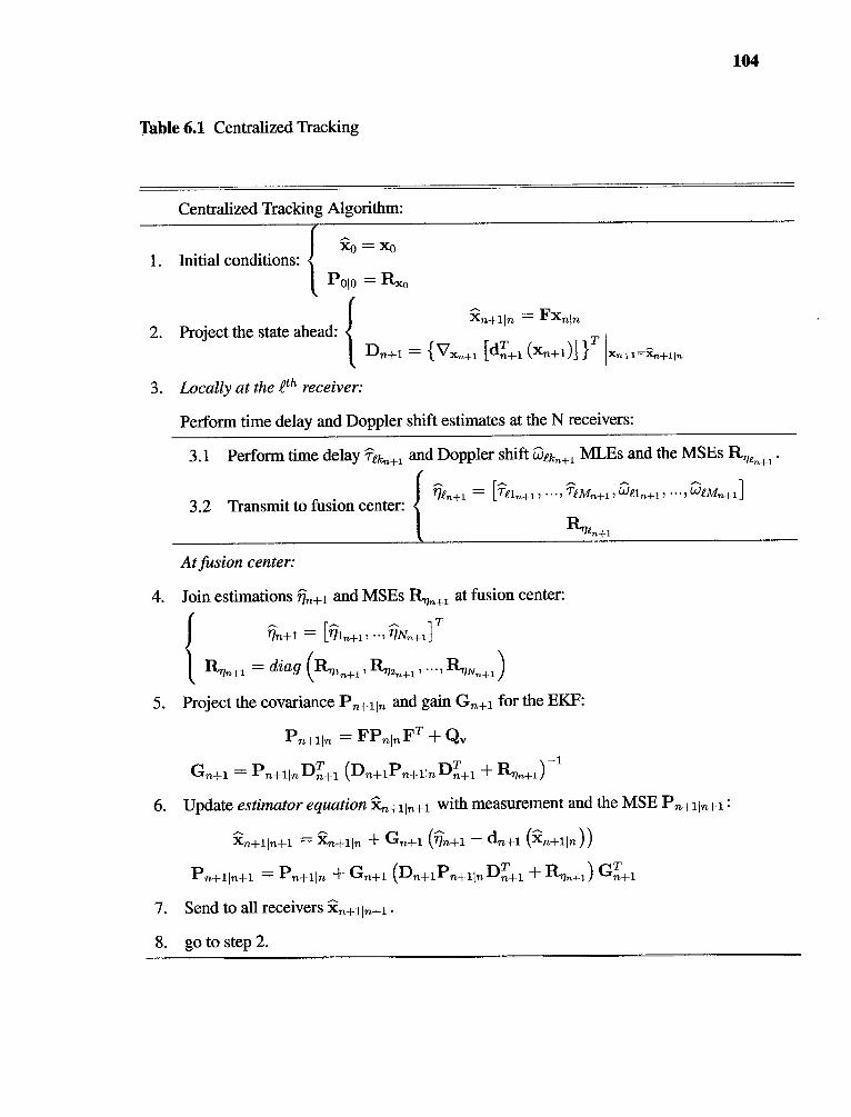
Table 6.1 Centralized Tracking
Centralized Tracking Algorithm:
1. Initial conditions:
2. Project the state ahead:
3. Locally at the eth receiver:
Perform time delay and Doppler shift estimates at the N receivers:
104
105
6.4.2 Decentralized Tracking
In decentralized tracking each receiving radars performs local estimates of the target
location and velocity using either direct MLE-based estimation of ict or indirect
estimation, i.e., first estimate = ..., , rjti, , (',.).em„,fi] and then
estimate ii,en+, using linearizion techniques. The projected or last updated target location
and velocity are used as a reference point in the linearizion process. The local estimates
are sent to a central fusion center, where they are combined based on a predetermined cost
function. The estimates are chosen such that path with significant fading or low reflectivity
will be either discarded of introduce with very high cost coefficients. By doing so, the
overall estimation MSE is kept as close as possible to the centralized performance. The
centralized algorithm is described in Table 6.2.
The centralized and decentralized algorithms performance are provided in Figure 6.9.
The proposed decentralized algorithm achieves accuracies very close to the centralized one.
The cost-based decentralized tracking method is shown to perform better than when all
paths a combined without any weighing coefficients (see Figure 6.10).
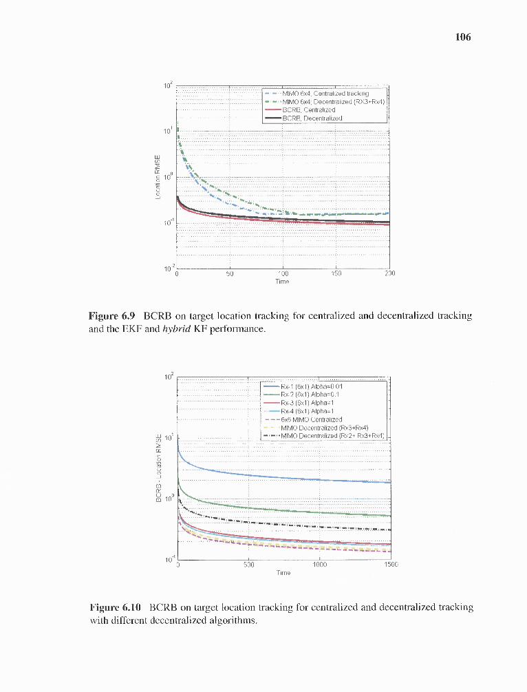
106
— 6x4, Centralized tracking—.—.•MIMO 6x4, Decentralized (RX3+Rx4)—BCRB, Centralized---,BCRB, Decentralized
Figure 6.9 BCRB on target location tracking for centralized and decentralized trackingand the EKF and hybrid KF performance.
Figure 6.10 BCRB on target location tracking for centralized and decentralized trackingwith different decentralized algorithms.

Table 6.2 Decentralized Tracking Algorithm
Decentralized Tracking:
1. Initial conditions:
2. Project the state ahead:
3. Locally at the fth receiver:
Perform target location
3.1 Perform time delay and Doppler shift MLEs.
3.3 Estimate target location and velocity based on local EKF.
3.4 To central fusion center:
At fusion center:
4. Perform target location :73-n+1 -re+1) and velocity In+i , -nd_1) estimates.:
4.1 Choose the best estimates by evaluating the covariance matrix
For a predetermined threshold, choose
4.2 Final estimation:
.ec{A.,}
where pe are the cost functions applied in combining the estimates,
and x is a threshold function, set to exclude the estimates with high MSEs.
5. Project the covariance Pn+iim and gain Gn+1 for the Kalman filter:
107
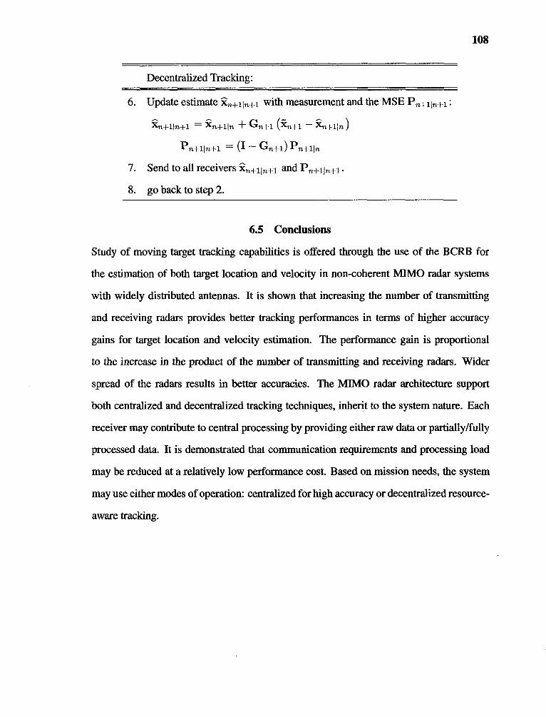
Decentralized Tracking:
108
6.5 Conclusions
Study of moving target tracking capabilities is offered through the use of the BCRB for
the estimation of both target location and velocity in non-coherent MEMO radar systems
with widely distributed antennas. It is shown that increasing the number of transmitting
and receiving radars provides better tracking performances in terms of higher accuracy
gains for target location and velocity estimation. The performance gain is proportional
to the increase in the product of the number of transmitting and receiving radars. Wider
spread of the radars results in better accuracies. The MIMO radar architecture support
both centralized and decentralized tracking techniques, inherit to the system nature. Each
receiver may contribute to central processing by providing either raw data or partially/fully
processed data. It is demonstrated that communication requirements and processing load
may be reduced at a relatively low performance cost. Based on mission needs, the system
may use either modes of operation: centralized for high accuracy or decentralized resource-
aware tracking.

CHAPTER 7
CONCLUSION AND FUTURE WORK
In the framework of this dissertation work, concepts of target localization in MIMO radar
systems with noncoherent and coherent processing were developed. Generally speaking,
MIMO radars with widely distributed transmit and receive antennas are addressed. The
main results discussed in the dissertation can be summarized as follows:
• The analytical expressions of the CRLB for noncoherent and coherent processing
were derived. For both noncoherent and coherent processing, an improvement in
target localization accuracy, proportional to the product of the number of transmitting
and receiving radars, MN, is obtained. This is referred to as spatial advantage.
• Location estimation based on noncoherent observations is shown to be inversely
proportional to the signals averaged effective bandwidth. Dramatically higher
accuracy can be obtained from processing coherent observations. In this case, the
estimation error is inversely proportional to the carrier frequency. This gain, in the
order of is due to the exploitation of phase information, and is referred to as
coherency advantage.
• Formulating a convex optimization problem, it is shown that symmetric deployment
of transmitting and receiving sensors around a target is optimal with respect to
minimizing the location estimation error on both x and y axis.
• Closed-form solution for the best linear unbiased estimator (BLUE) of target
localization is obtained for noncoherent and coherent MIMO radars. It supports the
use of the GDOP metric as a tool for target localization accuracy analysis. This
metric is shown to represent the spatial advantage of the system. Contour maps of
109
110
the GDOP, provide an insight of the mutual relation between a given deployment of
sensors and the achievable accuracy at various target locations.
• Comparative evaluation of target localization performances for MIMO and SIMO
radar systems, based on the BLUE is established. The advantage of the MIMO radar
scheme over SIMO is evident when considering that the achievable accuracy for
MIMO radar systems with M transmitters and N receivers is proportional to MN
and an equivalent SIMO radar systems with the same number of antennas, i.e. 1
transmitter and M + N — 1 receivers, is proportional to (M + N — 1), especially for
M N >> (M + N).
• Multiple targets localization, using coherent processing, is shown to benefit from
coherency advantage. The trade-off between target localization accuracy and the
number of targets that can be localized is incorporated in the spatial advantage term.
Increase in the number of targets exposes the system to elevated mutual interferences.
This trade-off depends on the geometric footprint of both the sensors and the targets,
and the relative positions of the two.
• Coherent processing advantage might be significant, for the ratio of the signal carrier
frequency to the signal effective bandwidth is commonly in the order of hundreds.
The reliance of coherent processing on phase synchronization initiated an analysis
that will evaluate the sensitivity of coherent localization to phase synchronization
errors. The bound on the target localization estimation error is shown to be a
sum of two terms — the first represents the CRB with no phase mismatch, and
the second captures the mismatch effect. The latter is shown to depend on the
phase error variance, the number of mismatched transmitting and receiving and
the system geometry. This expression provides the means to establish, for a
given phase synchronization error variance, if an advantage is still achievable for
coherent processing over noncoherent one. Alternatively, when system requirement

111
determined a specific localization accuracies, the derived expression may be used to
determine the necessary phase synchronization level in the distributed system.
• Study of moving target tracking capabilities of noncoherent MIMO radar systems is
performed through the use of the BCRB for the estimation of both target location
and velocity. It is shown that increasing the number of transmitting and receiving
radars provides alleviates tracking performances in terms of accuracy gains for both
location and velocity estimates. Performance gain is proportional to the increase in
the product of the number of transmitting and receiving radars. Wider spread of the
radars results in better accuracies.
• MIN40 radar architecture support both centralized and decentralized tracking
techniques, inherit to the system nature. Each receiver may contribute to central
processing by providing either raw data or partially/fully processed data. It is
demonstrated that communication requirements and processing load may be reduced
at a relatively low performance cost. Based on mission needs, the system may
use either modes of operation: centralized for high accuracy or decentralized
resource-aware tracking.
To fully gain from these systems some research and engineering challenges need to
be addressed. Among theses:
• Synchronization of the transmitting and receiving radars is of significant importance
to mapping performance. For non-coherent processing, time synchronization is
necessary while for coherent processing phase synchronization is required as well.
• Centralized coordination of sensor transmissions and waveforms design.
• Synchronized communication among radars and with a central processing center.
• Analysis of target RCS phenomena.

112
Traditionally, radar stations are grid-powered elements, incorporating transmitters,
receivers and fusion center on site, based on a fixed communication infrastructure. Over the
years, radar applications that include mobile deployment of stations were introduced, such
as anti-missiles defense radars. These systems are powered off-grid by diesel generators.
Other military applications require similar deployment of mobile stations for surveillance
of a given area, such as radars mounted on vehicles that have limited energy resources.
This type of systems utilizes secured wireless communication. In this case, the notion of
power aware design is very important.
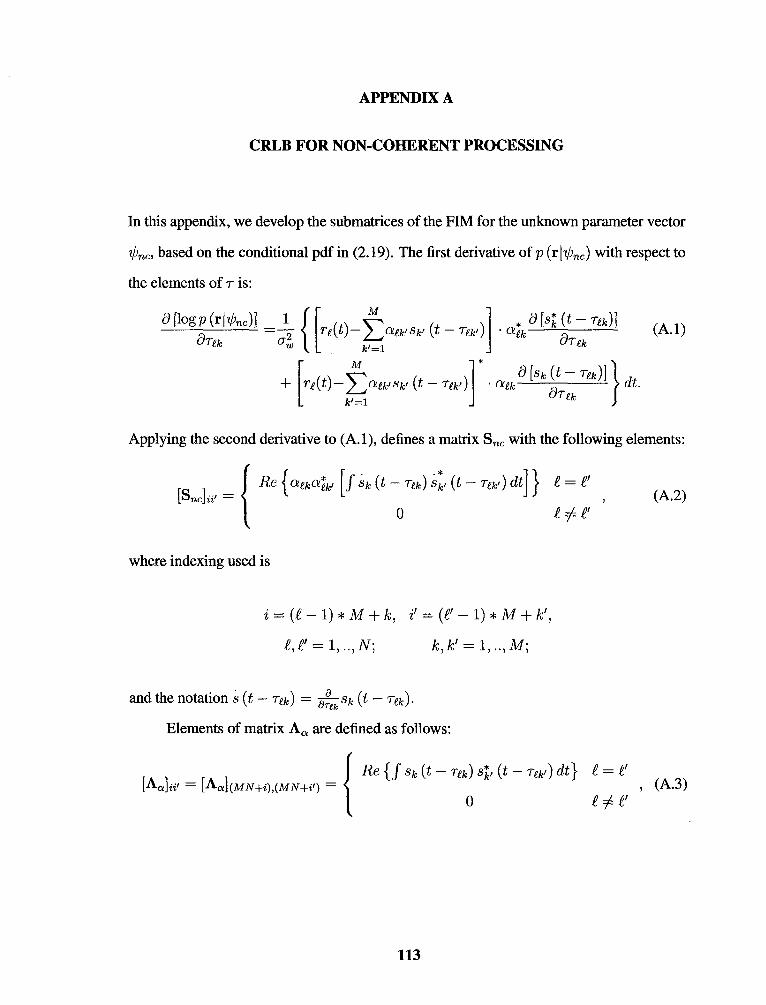
APPENDIX A
CRLB FOR NON-COHERENT PROCESSING
In this appendix, we develop the submatrices of the FIM for the unknown parameter vector
One, based on the conditional pdf in (2.19). The first derivative of p (r|ψnc) with respect to
the elements of T is:
(A.1)
Applying the second derivative to (A.1), defines a matrix Snc with the following elements:
(A.2)
where indexing used is
Elements of matrix Aa are defined as follows:
(A.3)
113
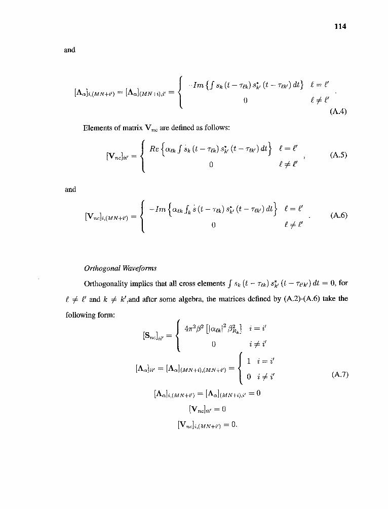
and
114
(A.4)
Elements of matrix V,, are defined as follows:
(A.5)
(A.6)
Orthogonal Waveforms
Orthogonality implies that all cross elements
e and k le,and after some algebra, the matrices defined by (A.2)-(A.6) take the
(A.7)
and

APPENDIX B
CRLB FOR COHERENT PROCESSING
In this appendix, we develop the submatrices of the FTM for the unknown parameter vector
, based on the conditional pdf in (2.34). The first derivative of p (0) with respect to
the elements of T is:
0 [log p (110c)]artk
Applying the second derivative to (B.1) define a matrix Sn, with the following elements:
(B.4)
(B.1)
(B.2)
(B.3)
Elements of matrix Aa, are defined as follows:
(B.5)
115
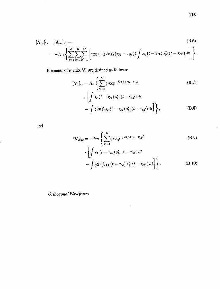
116
(B.6)
Elements of matrix V, are defined as follows:
(B.7)
(B.8)
(B.9)
(B.10)
and
Orthogonal Waveforms
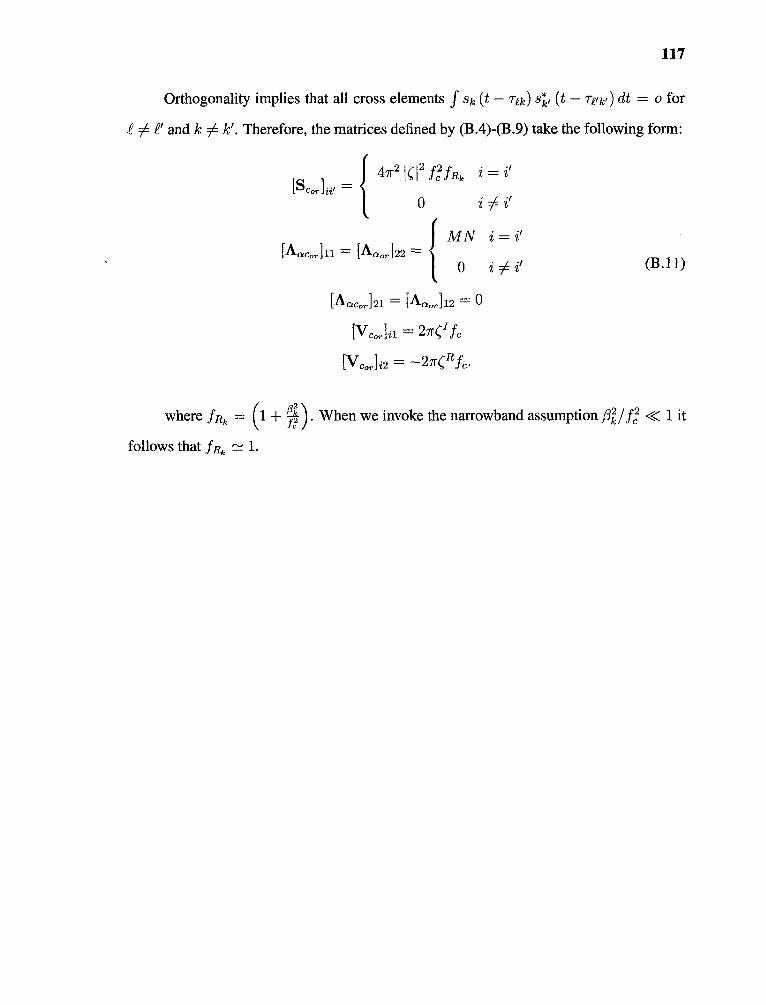
117
Orthogonality implies that all cross elements f sk (t — -roc) sZ, (t — re e) dt = o for
f' and k k'. Therefore, the matrices defined by (B.4)-(B.9) take the following form:
(B.11)
where fR, = (1 + (CO . When we invoke the narrowband assumption ,31g‹1 it
follows that fR, f_-_ 1.

APPENDIX C
DERIVATION OF ERROR COVARIANCE MATRIX FOR TIME OBSERVATIONS
C.1 Noncoherent Processing:
For a set of received waveforms re (t) , 1 < < N, in (2.10), the time delay estimates
/Inc == µnc12, • lincmNiT are determined by maximizing the following statistic:
(C.1)
by redefining the time notation t t — TA, where Tik denotes the propagation time on the
tic' path for the nominal point (xe, ye). Equivalently,
(C.2)
The time delay estimates are expressed in (3.3). It is not difficult to show that the following
relation holds:
(C.3)
where
(C.4)
and
(C.5)
We wish to write (C.3) in the form of (3.3). With a few algebraic manipulations, including(τlk
expanding gnc(v) in a Taylor series around τlk, and neglecting terms o [(τlk [(— µnclk)³],nclk)³] , it
can be shown that
(C.6)
118

119
Comparing this with (3.3), we have for the error term
(C.7)
To find the first and second order statistics of crice, , we need the statistical
characterization of ntk. As previously stated, we assume the receiver noise we (t) is a
Gaussian random process with zero mean and autocorrelation function o-2,6 (τ). Since na
is a linear transformation of the process wAt), since the mean wf(t) is zero, E [na] = 0.
Similarly, it can be shown that
(C.8)
(C.9)
concluding that the covariance matrix of the terms enclk is given by:
(C.10)
120
C.2 Coherent Processing
For a set of received waveforms re (t) , 1 < < N, in (2.8), the time delay estimatesT
µc = [µc11, µc12 " • 7 µcMN]T MN ] are determined by maximizing the following statistic:
(C.11)
by redefining the time notation t t — ilk, where rik denotes the propagation time on the
tkth path for the nominal point (x c, y e) . Equivalently,
(C.12)
The time delay estimates are expressed in (3.3). It is not difficult to show that the following
relation holds:
(C.111
where
(C.14)
and
(C.15)
With a few algebraic manipulations, including expanding g c(v) in a Taylor series around
F:ek, and neglecting terms o [(τlk — µclk, )³] , it can be shown that
(C.16)
Comparing this with (3.3), and invoking the narrowband assumption fiug 1, we have
for the error term
(C.17)
121
To find the first and second order statistics of c„ we need the statistical
characterization of ntk. As previously stated, we assume the receiver noise we(t) is a
Gaussian random process with zero mean and autocorrelation function au,' SM. Since nek
is a linear transformation of the process wi(t), since the mean we(t) is zero, E [flea] = 0.
Similarly, it can be shown that
(C.18)
(C.19)
concluding that the covariance matrix of the terms ectk is given by:
(C.20)
where SNRc =-- •
(D.2)
(D.3)
APPENDIX D
DERIVATION OF FIM MATRIX FOR PHASE SENSATIVITY ANALYSIS
In this appendix, we develop the FIM for the unknown parameter vector qp,
logp(r|ψ)
based on the conditional pdf in (4.14). The submatrices that define J =
E {ψ log p (r|ψ) log p (r|ψ))H} -E [a² logp(r|ψ)] are derived hereafter.(920
The submatrix rx, E, and V have the following general form:
(D.1)
The first derivative of p (1.11p) in (4.14) with respect to the elements of Tq is:
The following indexing notations are used throughout:
122
123
Applying the second derivative to (D.2) define the matrix rqqi with the following elements:
(D.4)
where 'go = 87²c SNR f²c .In matrix form,
(D.5)
where we define Aq = diag (0). The notation diag(-) is used to represent a
diagonal matrix with elements of vector (-) on its diagonal, eq is defined as eq =
[exp ( — fcqi) , exp ( — 27r fe4²c) , exp ( — 27r f crItIN)1T , and we abuse the notation and
let
(D.6)
The frequency ratio hi, is defined as A, = (1 + 110 . When we invoke the narrowband
assumption β²k/f²c << it follows that fR, 1.
The elements of matrix Its are defined as:
(D.7)
The second matrix E in (4.8) is defined by a set of matrices Eqq with the following
elements:
(D.8)
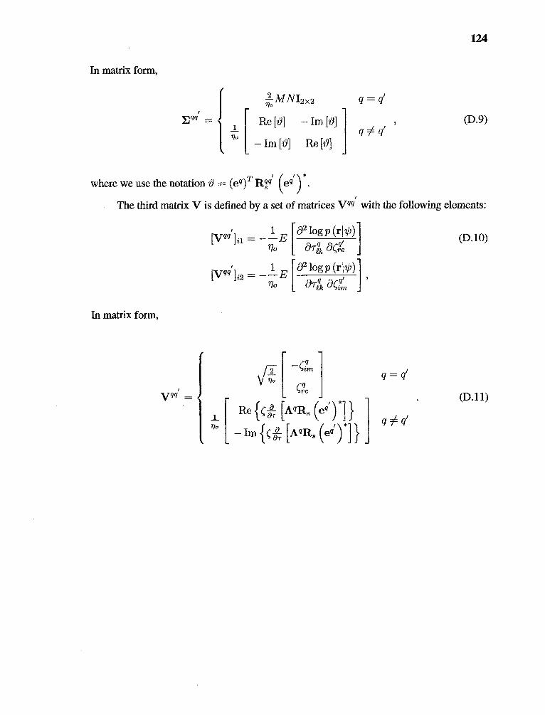
124
In matrix form,
(D.9)
where we use the notation 19 = (eq)T Rri (OD* .
The third matrix V is defined by a set of matrices Vqq/ with the following elements:
(D.10)
(D.11)
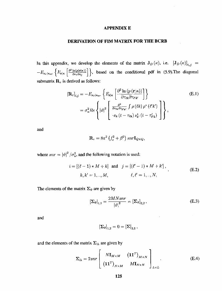
(E.2)
(E.3)
APPENDIX E
DERIVATION OF FIM MATRIX FOR THE BCRB
In this appendix, we develop the elements of the matrix JD (n), i.e. [JD
—E,1,,„, {Erik [°21anni:))1 }, based on the conditional pdf in (5.9).The diagonal
submatrix RT is derived as follows:
(E.1)
and
where snr = 1'191²c I o- , and the following notation is used:
The elements of the matrix E0 are given by
and
and the elements of the matrix EA are given by
(E.4)

and (E.b)
The off-diagonal submatrices are as follows:
126
(E.5)

REFERENCES
[1] A. Haimovich, R. Blum, and L. Cimini, "MIMO radar with widely separated antennas,"IEEE Signal Proc. Magazine, January 2008.
[2] E. Fishier, A. M. Haimovich, R. S. Blum, L. Cimini, D. Chizhik, and R. Valenzuela,"MIMO radar: An idea whose time has come," Processing of the 2004 IEEEInternational Conference on Radar, pp. 71-78, April 2004.
[3] H. Godrich, A. M. Haimovich, and R. S. Blum, Concepts and Applications of a MIMORadar System with Widely Separated Antennas. John Wiley, 2009.
[4] J. Li and P. Stoica, "MIMO radar with colocated antennas," IEEE Signal Proc. Magazine,pp. 106-114, September 2007.
[5] , "MIMO radar- diversity means superiority," Proc. 14th Annu. Workshop AdaptiveSensor Array Processing, pp. 123-127, June 2006.
[6] E. Fishier, A. Haimovich, R. Blum, L. Cimini, D. Chizhik, and R. Valenzuela,"Performance of MIMO radar systems: Advantages of angular diversity," Proc. 38thAsilomar Conf. Signals, Syst. Comput., pp. 305-309, November 2004.
[7] D. W. Bliss and K. W. Forsythe, "Multiple-input multiple-output (MIMO) radar andimaging: degrees of freedom and resolution," Proc. 37th Asilomar Conf. Signals, Syst.Comput., pp. 54-59, November 2003.
[8] J. Li, P. Stoica, and Y. Xie, "On probing signal design for MEMO radar," Proc. 40thAsilomar Conf. Signals, Syst. Comput., pp. 31-35, November 2006.
[9] F. C. Robey, S. Coutts, D. Weikle, J. C. McHarg, and K.Cuomo, "MIMO radar theory andexperimental results," Proc. 38th Asilomar Conf. Signals, Syst. Comput., pp. 300-304,November 2004.
[10] J. Tabrikian, "Barankin bounds for target localization by MIMO radars," Proc. 14th IEEEWorkshop on Sensor Array and Multi-Channel Pmcessing, pp. 278-281, July 2006.
[11] I. Bekkerman and J. Tabrildan, "Target detection and localization using MIMO radars andsonars," IEEE Trans. on Sig. Proc., vol. 54, pp. 3873-3883, October 2006.
[12] J. Li, P. Stoica, L. Xu, and W. Roberts, "On parameter identifiability of MIMO radar," IEEESignal Processing Lett., vol. 14, December 2007.
[13] L. Xu, J. Li, and d P. Stoica, "Adaptive techniques for MIMO radar," Proc. 14th IEEEWorkshop on Sensor Array and Multi-Channel Processing, pp. 278-281, July 2006.
[14] E. Fishier, A. Haimovich, R. Blum, L. Cimini, D. Chizhik, and R. Valenzuela, "Spatialdiversity in radars - models and detection performance," IEEE Trans. on Sig. Proc.,vol. 54, pp. 823-838, March 2006.
127
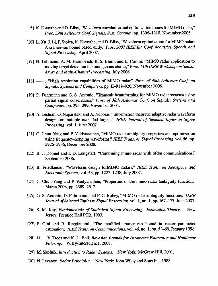
128
[15] K. Forsythe and D. Bliss, "Waveform correlation and optimization issues for MIMO radar,"Proc. 39th Asilomar Conf. Signals, Syst. Comput., pp. 1306-1310, November 2005.
[16] L. Xu, J. Li, P. Stoica, K. Forsythe, and D. Bliss, "Waveform optimization for mllvto radar:A cramer-rao bound based study," Proc. 2007 IEEE Int. Conf. Acoustics, Speech, andSignal Processing, April 2007.
[17] N. Lehmann, A. M. Haimovich, R. S. Blum, and L. Cimini, "MIMO radar application tomoving target detection in homogenous clutter," Proc. 14th IEEE Workshop on SensorArray and Multi-Channel Processing, July 2006.
[18] , "High resolution capabilities of MIMO radar," Proc. of 40th Asilomar Conf. onSignals, Systems and Computers, pp. II-917-920, November 2006.
[19] D. Fuhrmann and G. S. Antonio, "Transmit beamforming for MIMO radar systems usingpartial signal correlations," Proc. of 38th Asilomar Conf. on Signals, Systems andComputers, pp. 295-299, November 2004.
[20] A. Leshem, 0. Naparstek, and A. Nehorai, "Information theoretic adaptive radar waveformdesign for multiple extended targets," IEEE Journal of Selected Topics in SignalProcessing, vol. 1, June 2007.
[21] C. Chun-Yang and P. Vaidyanathan, "MIMO radar ambiguity properties and optimizationusing frequency-hopping waveforms," IEEE Trans. on Signal Processing, vol. 56, pp.5926-5936, December 2008.
[22] B. J. Donnet and I. D. Longstaff, "Combining mimo radar with ofdm communications,"September 2006.
[23] B. Friedlander, "Waveform design forMB,40 radars," IEEE Trans. on Aerospace andElectronic Systems, vol. 43, pp. 1227-1238, July 2007.
[24] C. Chun-Yang and P. Vaidyanathan, "Properties of the mimo radar ambiguity function,"March 2008, pp. 2309-2312.
[25] G. S. Antonio, D. Fuhrmann, and F. C. Robey, "MIIVIO radar ambiguity functions," IEEEJournal of Selected Topics in Signal Processing, vol. 1, no. 1, pp. 167-177, June 2007.
[26] S. M. Kay, Fundanzentals of Statistical Signal Processing: Estimation Theory. NewJersey: Prentice Hall PTR, 1993.
[27] E Gini and R. Reggiannini, "The modified cramer rao bound in vector parameterestimation," IEEE Trans. on Communications, vol. 46, no. 1, pp. 52-60, January 1998.
[28] H. L. V. Trees and K. L. Bell, Bayesian Bounds for Parameter Estimation and NonlinearFiltering. Wiley-Interscience, 2007.
[29] M. Skolnik, Introduction to Radar Systems. New York: McGraw-Hill, 2001.
[30] N. Levanon, Radar Principles. New York: John Wiley and Sons Inc, 1988.
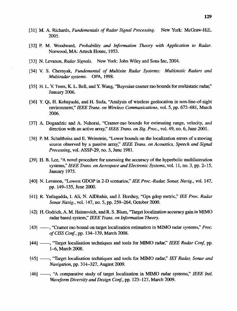
129
[31] M. A. Richards, Fundementals of Radar Signal Processing. New York: McGraw-Hill,2005.
[32] P. M. Woodward, Probability and Info. 'nation Theory with Application to Radar.Norwood, MA: Artech House, 1953.
[33] N. Levanon, Radar Signals. New York: John Wiley and Sons Inc, 2004.
[34] V. S. Chemyak, Fundemental of Multisite Radar Syatems: Multistatic Radars andMultiradar systems. OPA, 1998.
[35] H. L. V. Trees, K. L. Bell, and Y. Wang, "Bayesian cramer rao bounds for multistatic radar,"January 2006.
[36] Y. Qi, H. Kobayashi, and H. Suda, "Analysis of wireless geolocation in non-line-of-sightenvironment," IEEE Trans. on Wireless Communications, vol. 5, pp. 672-681, March2006.
[37] A. Dogandzic and A. Nehorai, "Cramer-rao bounds for estimating range, velocity, anddirection with an active array," IEEE Trans. on Sig. Proc., vol. 49, no. 6, June 2001.
[38] P. M. Schultheiss and E. Weinstein, "Lower bounds on the localization errors of a movingsource observed by a passive array," IEEE Trans. on Acoustics, Speech and SignalProcessing, vol. ASSP-29, no. 3, June 1981.
[39] H. B. Lee, "A novel procedure for assessing the accuracy of the hyperbolic multilaterationsystems," IEEE Trans. on Aerospace and Electronic Systems, vol. 11, no. 3, pp. 2-15,January 1975.
[40] N. Levanon, "Lowest GDOP in 2-D scenarios," IEE Proc.-Radar, Sonar Navig., vol. 147,pp. 149-155, June 2000.
[41] R. Yarlagadda, I. Ali, N. AlDhahir, and J. Hershey, "Gps gdop metric," IEE Proc. RadarSonar Navig., vol. 147, no. 5, pp. 259-264, October 2000.
[42] H. Godrich, A. M. Haimovich, and R. S. Blum, "Target localization accuracy gain in MIMOradar based system," IEEE Trans. on Information Theory.
[43] , "Cramer rao bound on target localization estimation in MIMO radar systems," Proc.of CISS Conf., pp. 134-139, March 2008.
[44] , "Target localisation techniques and tools for MIMO radar," IEEE Radar Conf, pp.1-6, March 2008.
[45] , "Target localisation techniques and tools for MIMO radar," IET Radar, Sonar andNavigation, pp. 314-327, August 2009.
[46] , "A comparative study of target localization in MIMO radar systems," IEEE Intl.Waveform Diversity and Design Conf., pp. 123-127, March 2009.
130
[47] , "Target localization accuracy and multiple target localization: Tradeoff in MIMOradars," Proc. of 42th Asilomar Conf. Signals, Syst. Comput., pp. 614-618, October2008.
[48] H. Godrich, A. M. Haimovich, and H. V. Poor, "An analysis of phase synchronizationmismatch sensitivity for coherent MIMO radar systems," To appear in Proc. of theThird International Workshop on Computational Advances in Multi-Sensor AdaptiveProcessing (CAMSAP), December 2009.
[49] Q. He, R. S. Blum, H. Godrich, and A. M. Haimovich, "Cramer-rao bound for targetvelocity estimation in MIMO radar with widely separated antennas," Proc. of 42ndAnnual Conference on Information Sciences and Systems (CISS), pp. 123-127, March2008.
[50] , "Target velocity estimation and antenna placement for mimo radar with widelyseparated antennas," IEEE Journal of Selected Topics in Signal Processing.
[51] H. Godrich, A. M. Haimovich, and R. S. Blum, "A MIMO radar system approach totarget tracking," To appear in Proc. of 43th Asilomar Conf. Signals, Syst. Comput.,November 2009.
[52] , "Target tracking in MIMO radar systems: Techniques and performance analysisradar," submitted to IEEE Radar Conf, May 2010.
[53] J. Minkoff, Signal Processing Fundamentals and Applications for Communications andSensing Systems. Artech House, 2002.
[54] D. R. B. III, G. B. Prince, and J. A. McNeill, "Time-slotted round-trip aarriersynchronization for distributed beamfonning," IEEE Trans. on Signal Processing,vol. 56, no. 11, pp. 5630-5643, November 2008.
[55] Y. S. Tu and G. J. Pottie, "Coherent cooperative transmission from multiple adjacentantennas to a distant stationary antenna through AWGN channels," Proc. IEEE VTC02, pp. 130-134,2002.
[56] G. Baniac, R. Mudumbai, and U. Madhow, "Distributed beamforming for informationtransfer in sensor networks," Proc. of the Third International Symposium onInformation Processing in Sensor Networks, pp. 81-88,2004.
[57] S. Berger and A. Wittneben, "Carrier phase synchronization of multiple distributed nodes ina wireless network," 8th IEEE Workshop on Signal Processing Advances for WirelessCommunications (SPAWC)s, June 2007.
[58] W. Wang, C. B. Ding, and X. D. Liangl, "Time and phase synchronisation via direct-pathsignal for bistatic synthetic aperture radar systems," IET Radat; Sonar and Navigation,vol. 2, pp. 1-11, February 2008.
131
[59] P. Napier, A. R. Thompson, and R. D. Ekers, "The very large array: Design andperformance of a modern synthesis radio telescope," IEEE Proc., vol. 71, no. 11, pp.1295-1320, November 1983.
[60] B. D. Steinberg, "Phase synchronizing a nonrigid, distributed, transmit-receive radarantenna array," IEEE Trans. on Aero. and Elect. Systems, vol. AES-18, pp. 609-620,September 1982.
[61] B. D. Steinberg, W. Whistler, and D. Carlson, "Two-dimensional imaging with a radiocamera," IEEE Proc, vol. 71, pp. 1325-1326, November 1983.
[62] B. M. Keel and T. H. Heath, "A comprehensive review of quasi-orthogonal waveforms:'Proc. of 38th Asilomar Conf on Signals, Systems and Computers, pp. 122-127, April2007.
[63] S. Boyd and L. Vandenberghe, Convex Optimization. Cambridge Press, 2004.
[64] V. D. Blondel, S. Boyd, and H. Kimurae, Recent Advances in Learning and Control.Springer, 2008.
[65] H. V. Poor, An Introduction to Signal Detection and Estimation, 2nd ed. New York:Springer, 1994.
[66] E. Weinstein and A. Weiss, "Fundemental limitation in passive time-delay estimation-partii: wide -band systems," IEEE Trans. on Acoustics, Speech and Signal Proc., vol.ASSP-32, no. 5, pp. 1064-1078, October 1984.
[67] A. Zeira and P. M. Schultheiss, "Realizable lower bounds for time delay estimation," IEEETrans. on Signal Processing, vol. 41, no. 11, November 1993.
[68] M. Hamilton and P. M. Schultheiss, "Passive ranging in mulyipath dominant environment,part i: Known multipath parameters," IEEE. trans on Signal Proc., vol. 40, no. 1,January 1992.
[69] Y. Rockah and P. M. Schultheiss, "Array shape calibration using sources in unknownlocations - part i: Far-field sources," IEEE Trans. Acoust., Speech, Signal Proc., vol.Vol. ASSP-35, pp. 286-299, March 1987.
[70] Y. Rockah, H. Messer, and P. M. Schultheiss, "Localization performance of arrays subjectto phase en-ors," IEEE Trans. Acoust., Speech, Signal Proc., vol. ASSP-35, no. 8, pp.286-299, March 1987.
[71] R. A. Horn and C. R. Johnson, Matrix Analysis. Cambridge UK: Cambridge UniversityPress„ 1990.
[72] K. S. Miller, "On the inverse of the sum of matrices," Mathematics Magazine, vol. 54,no. 2, pp. 67-72,1981.
[73] Y. Bar-Shalom, X. R. Li, and T. Kirubarajan, Estimation with Applications to Tracking andNavigation. NewYork, NY: John Wiley and sons, 2001.

132
[74] L. D. Stone, C. A. Barlow, and T. L. Corwin, Bayesian Multiple Target Tracking.Norwood, MA: Artech House, Inc, 1999.
[75] a. P. S. Blackman, Modern Tracking Systems. Norwood, MA: Artech Hounse, 1999.
[76] P. Tichavsky, C. H. Muravchik, and A. Nehorai, "Posterior cramer-rao bounds for discrete-time nonlinear filtering," IEEE Trans. Signal Processing, vol. 46, no. 5, pp. 1386—1396, May 1998.
[77] H. L. V. Trees, K. L. Bell, and Y. Wang, "Bayesian cramer-rao bounds for multistatic radar,"Proc. Of IEEE WDD Conf., May 2006.
[78] R. E. Zarnich, K. L. Bell, and H. L. V. Trees, "A unified method for measurement andtracking of contacts from an array of sensors," IEEE Trans. Signal Processing, vol. 49,no. 12, pp. 2950-2961, December 2001.


