
Chapter 7: Variances
In this chapter we consider a variety of exten-
sions to the linear model that allow for more gen-
eral variance structures than the independent, iden-
tically distributed errors assumed in earlier chap-

ters. This greatly extends the problems to which
linear regression can be applied.

1 Weighted least squares
The assumption that the variance function Var(Y |X)
is the same for all values of the terms X can be re-
laxed as follows.
Var(Y |X = xi) = Var(ei) = σ2/wi,
where w1, . . . , wn are known positive numbers.
This leads to the use of weighted least squares, or
WLS, in place of OLS, to get estimates.

In matrix terms, the model can be written as
Y = Xβ + e, Var(e) = σ2W−1. (1)
The estimator β is chosen to minimize the weighted
residual sum of squares function,
RSS(β) = (Y −Xβ)′W (Y −Xβ)
=∑
i
wi(yi − xiβ)2.
The WLS estimator is given by
β = (X ′WX)−1X ′Wy.

Let W 1/2be the n × n diagonal matrix with
ith diagonal element√wi, and so W−1/2
is a di-
agonal matrix with 1/√wi on the diagonal. De-
fine Z = W 1/2Y , M = W 1/2X , and d =
w1/2e, and (1) is equivalent to
Z = Mβ + d. (2)
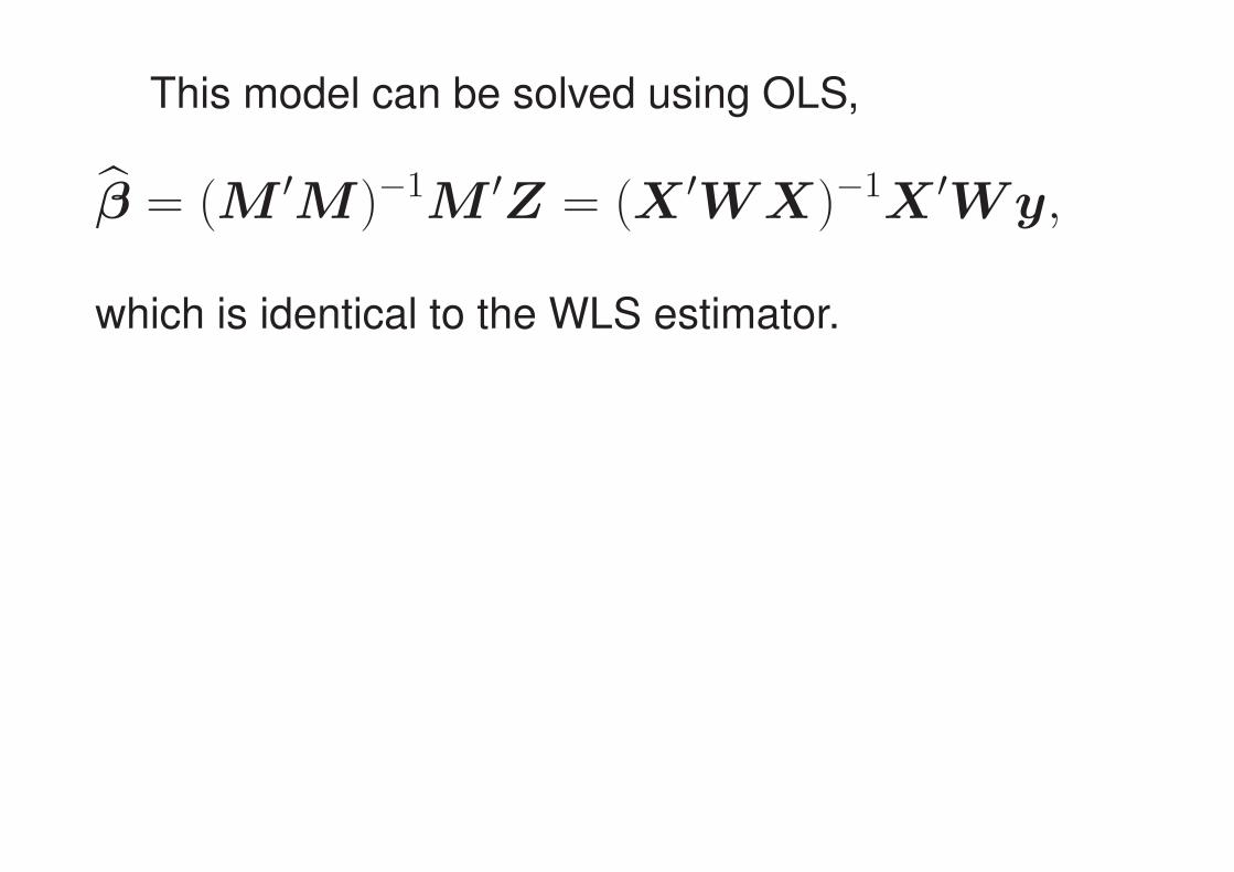
This model can be solved using OLS,
β = (M ′M )−1M ′Z = (X ′WX)−1X ′Wy,
which is identical to the WLS estimator.

1.1 Applications of weighted least squares
Known weight wi can occur in many ways. If the
ith response is an average of ni equally variable
observations, then Var(yi) = σ/ni, and wi = ni.
If yi is a total of ni observations, Var(yi) = niσ2,
andwi = 1/ni. If variance is proportional to some
predictor xi, Var(yi) = xiσ2, then wi = 1/xi.
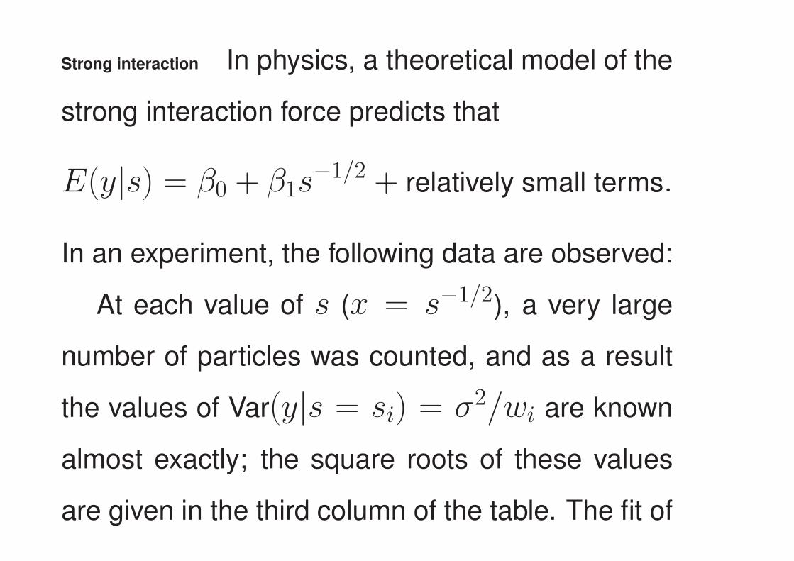
Strong interaction In physics, a theoretical model of the
strong interaction force predicts that
E(y|s) = β0 + β1s−1/2 + relatively small terms.
In an experiment, the following data are observed:
At each value of s (x = s−1/2), a very large
number of particles was counted, and as a result
the values of Var(y|s = si) = σ2/wi are known
almost exactly; the square roots of these values
are given in the third column of the table. The fit of

Table 1: The strong interaction data.
No. x y SD
1 0.345 367 17
2 0.287 311 9
3 0.251 295 9
4 0.225 268 7
5 0.207 253 7
6 0.186 239 6
7 0.161 220 6
8 0.132 213 6
9 0.084 193 5
10 0.060 192 5

the simple regression model via WLS is summa-
rized in Table 2. R2 is large, and the parameter
estimates are well determined.

Table 2: WLS estimates for the strong interaction data.
Coefficients:
Estimate Std. Error t value Pr(>|t|)
(Intercept) 148.473 8.079 18.38 7.91e-08
x 530.835 47.550 11.16 3.71e-06
Residual standard error: 1.657 on 8 degrees of freedom
Multiple R-Squared: 0.9397, Adjusted R-squared: 0.9321
F-statistic: 124.6 on 1 and 8 DF, p-value: 3.710e-06
Analysis of Variance Table
Df Sum Sq Mean Sq F value Pr(>F)
x 1 341.99 341.99 124.63 3.710e-06 ***
Residuals 8 21.95 2.74

2 Misspecified Variances
Suppose the true regression model is
E(Y |X) = Xβ, Var(Y |X) = σ2W−1,
where W has positive weights on the diagonal
and zeros elsewhere. We get the weights wrong,
and fit the model using OLS with the estimator
β0 = (X ′X)−1X ′Y .

Similar to the correct WLS estimate, this estimator
is unbiased, E(β0|X) = β. However, the vari-
ance is
Var(β0|X) = σ2(X ′X)−1(X ′W−1X)(X ′X)−1.

2.1 Accommodating misspecified variance
To estimate Var(β0|X) requires estimating σ2W−1.
Let ei = yi−β′0xi be the ith residual from the mis-
specified model. Then e2i is an estimate of σ2/wi.
It has been shown that replacing σ2W−1by a di-
agonal matrix with the e2i on the diagonal produces
a consistent estimate of Var(β0|X).
Several variations of this estimate that are equiv-
alent in large samples but have better small sam-

ple behavior have been proposed. For example,
one estimate, often called HC3, is
Var(β0|X) = (X ′X)−1
[X ′diag
(e2i
(1− hii)2
)X
]
(X ′X)−1,
where hii is the ith leverage. An estimator of this
type is often called a sandwich estimator.

Table 3: Sniffer data estimates and standard errors
OLS Estimate OLS SE HC3 SE
(Intercept) 0.15391 1.03489 1.047
TankTemp -0.08269 0.04857 0.044
GasTemp 0.18971 0.04118 0.034
TankPres -4.05962 1.58000 1.972
GasPres 9.85744 1.62515 2.056
2.2 A Test for Constant Variance
Suppose that for some parameter vector λ and
some vector of regressors Z
Var(Y |X,Z = z) = σ2 exp(λ′z), (3)

where the weights are given by w = exp(−λ′z).
If λ = 0, then (3) corresponds to constant vari-
ance. Hence, a test of NH: λ = 0 versus AH :
λ 6= 0 is a test for nonconstant variance. There is
a great latitude in specifying Z. If Z = Y , then
the variance depends on the response. Similarly,
Z may be the same as X or a subset of X .
Assume normal errors, a score test can be used,
for which the test statistic has an approximateχ2(q)
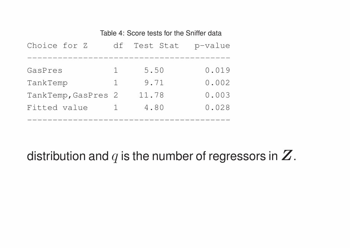
Table 4: Score tests for the Sniffer data
Choice for Z df Test Stat p-value
----------------------------------------
GasPres 1 5.50 0.019
TankTemp 1 9.71 0.002
TankTemp,GasPres 2 11.78 0.003
Fitted value 1 4.80 0.028
----------------------------------------
distribution and q is the number of regressors inZ .

3 General Correlation Structures
The generalized least squares or GLS model ex-
tends WLS one step further, and starts with
E(Y |X) = Xβ, Var(Y |X) = Σ,
where Σ is an n × n positive definite symmetric
matrix. The WLS model uses Σ = σ2W−1for
a diagonal matrix W , and the OLS model uses
Σ = σ2I.

If we have n observations and Σ is completely
unknown, then Σ contains n(n − 1)/2 parame-
ters, which is much larger than the number of ob-
servations n. The only hope is to introduce some
structure in Σ. Here are some examples.

Compound Symmetry If all the observations are equally
correlated, then
ΣCS = σ2
1 ρ · · · ρ
ρ 1 · · · ρ...
.... . .
...
ρ ρ · · · 1
,
which has only two parameters ρ and σ2. Gen-
eralized least squares software, such as the gls
function in the nlme package, can be used for es-

timation.
Autoregressive This form is generally associated with
time series. If data are time ordered and equally
spaced, the lag-1 autoregressive covariance struc-

ture is
ΣAR = σ2
1 ρ · · · ρn−1
ρ 1 · · · ρn−2
......
. . ....
ρn−1 ρn−2 · · · 1
,
which also contains only two parameters.
Block Diagonal A block diagonal form for Σ can arise
if observations are sampled clusters. For exam-
ple, a study of school performance might sample

m children from each of k classrooms. The m
children within a classroom may be correlated be-
cause they all have the same teacher, but children
in different classrooms are independent.

4 Random Coefficient Models
The random coefficient model, as special case of
mixed models, allows for appropriate inferences.
Consider a population regression mean function
E(y|loudness = x) = β0 + β1x,
where subject effects are not allowed. To add them
we hypothesize that each of the subjects may have
his or her own slope and intercept. Let yij, i =

1, . . . , 10, j = 1, . . . , 5 be the log-response for
subject i measured at the jth level of loudness.
For the ith subject,
E(yij|loudness = x, b0i, b1i) = (β0 + b0i)
+ (β1 + b1i)loudnessij.
where b0i and b1i are the deviations from the pop-
ulation intercept and slope for the ith subject, and

they are treated as random variables,(b0i
b1i
)∼ N
((0
0
),
(τ 20
τ01
τ01 τ 21
)).
Inferences about (β0, β1) concern population be-
havior. Inferences about (τ 20, τ 2
1) concern the vari-
ation of the intercepts and slopes between individ-
uals in the population.

5 Variance Stabilizing Transformation
Suppose that the response is strictly positive, and
the variance function before transformation is
Var(Y |X = x) = σ2g(E(Y |X = x)),
where g(E(Y |X = x)) is a function that is in-
creasing with the value of its argument. For exam-
ple, if the distribution of Y |X has a Poisson distri-
bution, then g(E(Y |X = x)) = E(Y |X = x).

For distributions in which the mean and vari-
ance are functionally related, Scheffe (1959) pro-
vides a general theory for determining transforma-
tions that can stabilize variance. Table 5 lists the
common variance stabilizing transformations.

YT Comments√Y Used when Var(Y |X) ∝ E(Y |X), as for Poisson distributed data. YT =√
Y +√Y + 1 can be used if all the counts are small.
log(Y ) Used if Var(Y |X) ∝ [E(Y |X)]2. In this case, the errors behave like a
percentage of the response, ±10%, rather than an absolute deviation, ±10
units.
1/Y The inverse transformation stabilizes variance when Var(Y |X) ∝[E(Y |X)]4. It can be appropriate when responses are mostly close to 0,
but occasional large values occur.
sin−1(√Y ) The arcsine square-root transformation is used if Y is a proportion between
0 and 1, but if can be used more generally if y has a limited range by first
transforming Y to the range (0,1), and then applying the transformation.
Table 5: Common variance stabilizing transformations.

6 The Delta Method
As a motivation example, we consider a polyno-
mial regression. If the mean function with one pre-
dictor X is smooth but not straight, integer pow-
ers of the predictors can be used to approximate
E(Y |X). The simplest example of this is quadratic
regression, in which the mean function is
E(Y |X = x) = β0 + β1x + β2x2. (4)

Quadratic mean functions can be used when the
mean is expected to have a minimum or maximum
in the range of the predictor. The minimum or max-
imum will occur for the value of X for which the
derivative dE(Y |X = x)/dx = 0, which occurs
at
xM = −β1/(2β2). (5)
The delta methods provides an approximate stan-
dard error of a nonlinear combination of estimates

that is accurate in large samples.
Suppose g(θ) is a nonlinear continuous func-
tion of θ, θ∗is the true value of θ, and θ is the
estimate. It follows from Taylor series expansion
that
g(θ) = g(θ∗) +k∑
j=1
∂g
∂θj(θj − θ∗j ) + small terms
≈ g(θ∗) + g(θ∗)′(θ − θ∗),

where g(θ∗) = ( ∂g∂θ1
, · · · , ∂g∂θ1
)′. It implies that
Var(g(θ)) ≈ g(θ∗)′Var(θ)g(θ∗).
For quadratic regression (4), the minimum or maxi-
mum occurs at g(β) = −β1/(2β2), which is esti-
mated by g(β). A straightforward calculation gives
Var(g(β)) =1
4β2
2
(Var(β1) +
β2
1
β2
2
Var(β2)−
2β1
β2Cov(β1, β2)
),
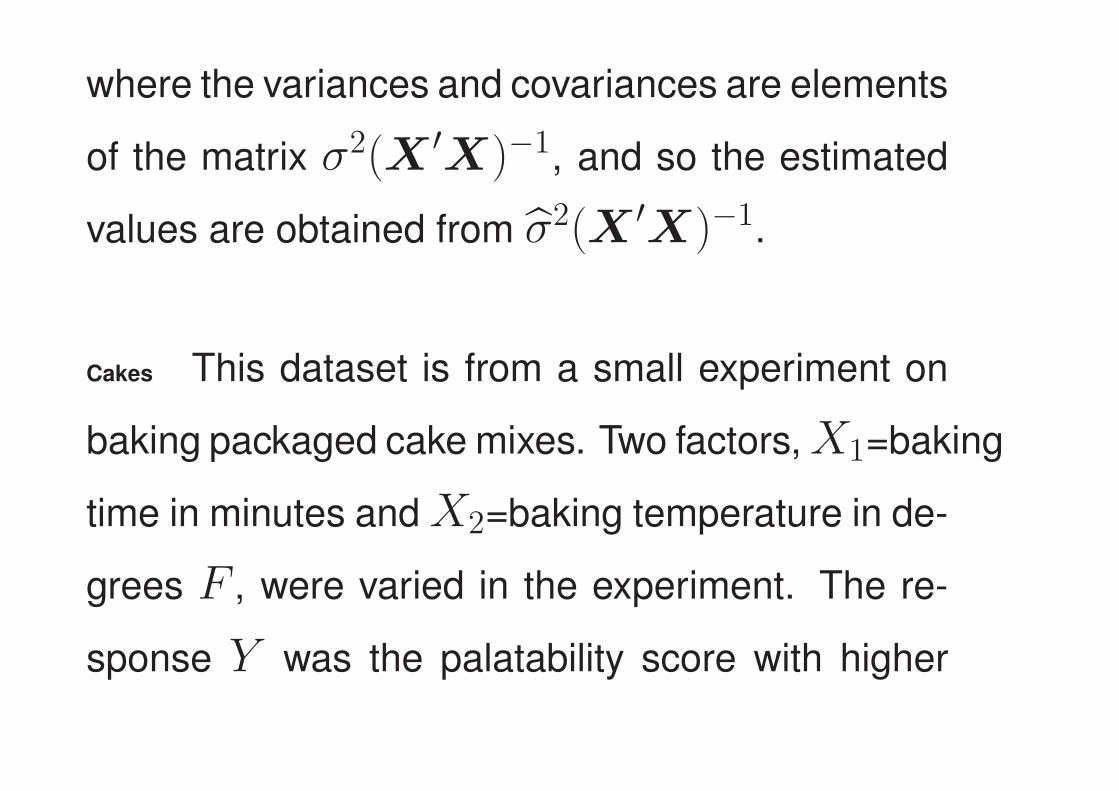
where the variances and covariances are elements
of the matrix σ2(X ′X)−1, and so the estimated
values are obtained from σ2(X ′X)−1.
Cakes This dataset is from a small experiment on
baking packaged cake mixes. Two factors, X1=baking
time in minutes and X2=baking temperature in de-
grees F , were varied in the experiment. The re-
sponse Y was the palatability score with higher

values desirable. The estimated mean function is
E(Y |X1, X2) = −2204.4850 + 25.91976X1+
9.9183X2 − 0.1569X2
1− 0.0120X2
2− 0.0416X1X2.
When the temperature is set to 350, the estimated
maximum palatability occurs when the baking time
is
xM = −β1 + β12(350)
2β11= 36.2.
The standard error from the delta method can be
computed to be 0.4 minutes. If we can believe the

normal approximation, a 95% confidence interval
for xM is 36.2 ± 1, 96 × 0.4 or about 35.4 to 37
minutes.

7 The Bootstrap
Suppose we have a sample y1, . . . , yn from a par-
ticular distribution G, for example a standard nor-
mal distribution. What is a confidence interval for
the population median?
We can obtain an approximate answer to this
question by computer simulation, set up as follows.
1. Obtain a simulated random sample y∗1, . . . , y∗n
from the known distribution G.

2. Compute and save the median of the sample
in step 1.
3. Repeat steps 1 and 2 a large number of times,
say B times. The larger the value of B, the
more precise the ultimate answer.
4. If we takeB = 999, a simple percentile-based
95% confidence interval for the median is the
interval between the sample 2.5 and 97.5 per-
centiles, respectively.

In most interesting problems, G is unknown and
so this simulation is not available. Efron (1979)
pointed out that the observed data can be used
to estimate G, and then we can sample from the
estimate G. The algorithm becomes:
1. Obtain a random sample y∗1, . . . , y∗n from G
by sampling with replacement from the observed
values y1, . . . , yn. In particular, the i-th ele-
ment of the sample y∗i is equally likely to be

any of the original y1, . . . , yn. Some of the yi
will appear several times in the random sam-
ple, while others will not appear at all.
2. Continue with steps 2-4 of the first algorithm.
A test at the 5% level concerning the popu-
lation median can be rejected if the hypothe-
sized value of the median does not fall in the
confidence interval computed in step 4.
Efron called this method the bootstrap.

7.1 Regression Inference without Normality
For regression problems, when the sample size
is small and the normality assumption does not
hold, standard inference methods can be mislead-
ing, and in these cases a bootstrap can be used
for inference.
Transactions Data Each branch makes transactions of
two types, and for each of the branches we have
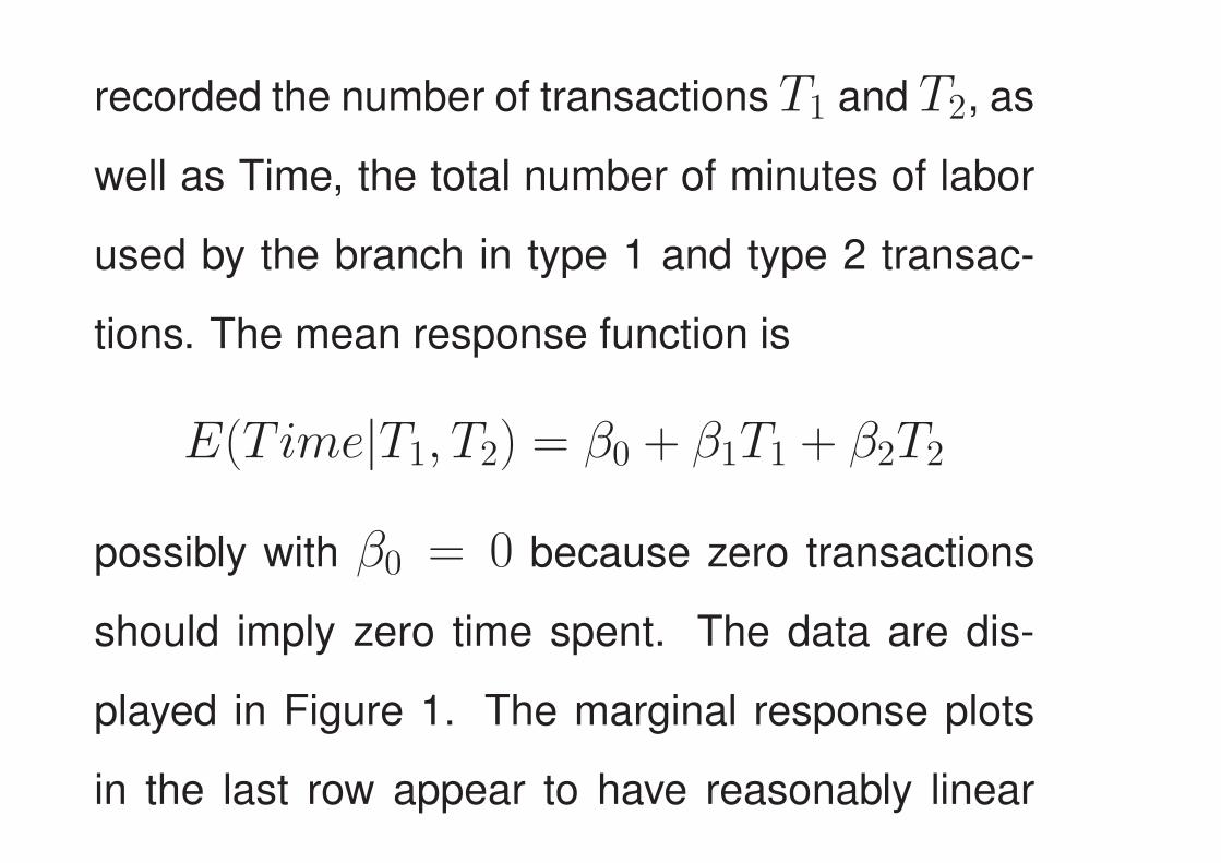
recorded the number of transactions T1 and T2, as
well as Time, the total number of minutes of labor
used by the branch in type 1 and type 2 transac-
tions. The mean response function is
E(T ime|T1, T2) = β0 + β1T1 + β2T2
possibly with β0 = 0 because zero transactions
should imply zero time spent. The data are dis-
played in Figure 1. The marginal response plots
in the last row appear to have reasonably linear

mean functions; there appear to be a number of
branches with no T1 transactions but many T2 trans-
actions; and in the plot of Time versus T2, variabil-
ity appears to increase from left to right.
The errors in this problem probably have a skewed
distribution. Occasional transactions take a very
long time, but since transaction time is bounded
below by zero, there cannot be any really extreme
“quick” transactions. Inferences based on normal

T1
0 1000 2000 3000 4000 5000 6000
0500
1000
1500
01000
2000
3000
4000
5000
6000
T2
0 500 1000 1500 0 5000 10000 15000 20000
05000
10000
15000
20000
Time
Figure 1: Scatterplot matrix for the transactions data.
theory are therefore questionable.
A bootstrap is computed as follows.
1. Number the cases in the dataset from 1 to
n. Take a random sample with replacement
of size n from these case numbers.
2. Create a dataset from the original data, but
repeating each row in the dataset the number
of times that row was selected in the random
sample in step 1.

3. Repeat steps 1 and 2 a large number of times,
say, B times.
4. Estimate a 95% confidence interval for each of
the estimates by the 2.5 and 97.5 percentiles
of the sample of B bootstrap samples.
Table 6 summarizes the percentile bootstrap for
the transaction data.
The 95% bootstrap intervals are consistently wider
than the corresponding normal intervals, indicat-

Table 6: Summary for B = 999 case bootstraps for the transactions data.
Normal Theory Bootstrap
Estimate Lower Upper Estimate Lower Upper
Intercept 144.37 -191.47 480.21 136.09 -254.73 523.36
T1 5.46 4.61 6.32 5.48 4.08 6.77
T2 2.03 1.85 2.22 2.04 1.74 2.36
ing that the normal-theory confidence intervals are
probably overly optimistic.

7.2 Nonlinear functions of parameters
One of the important uses of the bootstrap is to
get estimates of error variability in problems where
standard theory is either missing, or, equally of-
ten, unknown to analyst. Suppose, for example,
we wanted to get a confidence interval for the ra-
tio β1/β2 in the transactions data. The point es-
timate for this ratio is just β1/β2, but we will not
learn how to get a normal-theory confidence inter-

val for a nonlinear function of parameters like this
until Chapter 6.
Using bootstrap, this computation is easy: just
compute the ratio in each of the bootstrap samples
and then use the percentiles of the bootstrap dis-
tribution to get the confidence interval. For these
data, the point estimate is 2.68 with 95% confi-
dence interval from 1.76 to 3.86.


